performance prediction of pm 2.5 removal of real fibrous

1

Performance prediction of PM 2.5 removal of real fibrous filters with 1

a novel model considering rebound effect 2

3

Rong-Rong Cai1, Li-Zhi Zhang1, Yuying Yan2 4

5

1Key Laboratory of Enhanced Heat Transfer and Energy Conservation of Education Ministry, 6

School of Chemistry and Chemical Engineering, South China University of Technology, 7

Guangzhou 510640, PR China 8

2Fluids & Thermal Engineering Research Group, Faulty of Engineering, University of 9

Nottingham, Nottingham NG7 2RD, UK 10

11

Abstract: Fibrous filters have been proved to be one of the most cost-effective way of 12

particulate matters (specifically PM 2.5) purification. However, due to the complex structure 13

of real fibrous filters, it is difficult to accurately predict the performance of PM2.5 removal. In 14

this study, a new 3D filtration modeling approach is proposed to predict the removal 15

efficiencies of particles by real fibrous filters, by taking the particle rebound effect into 16

consideration. A real filter is considered and its SEM image-based 3D structure is established 17

for modeling. Then based on the simulation result, the filtration efficiency and pressure drop 18

are calculated. The obtained values are compared and validated by experimental data and 19

empirical correlations, and the results are proven to be in good agreement with each other. At 20

last, influences of various parameters including the face velocity, particle size and the particle 21

rebound effect on the filtration performance of fibrous filters are investigated. The results 22

Author for correspondence. Tel/fax: 86-20-87114264; Email: [email protected]

mailto:[email protected]

2

provide useful guidelines for the optimization and enhancement of PM2.5 removal by fibrous 1

filter. 2

3

Keywords: PM2.5; filtration performance; fibrous filter; particle rebound; Micro-macro 4

modeling; material property 5

6

1. Introduction 7

Particulate matter (PM) pollution has adverse effects on visibility, direct and indirect 8

radiative forcing, climate, and ecosystems [1-3]. Airborne particulate matter (including PM2.5) 9

is a diverse pollutant class whose excessive presence in indoor air contributes to an array of 10

adverse health and material damage effects [4]. Numerous particle filtration techniques have 11

been developed to reduce the concentrations of airborne particles in indoor air in the past 12

decades [5, 6]. Fibrous filters, which are commonly used in theses particle filtration systems, 13

have been regarded as one of the most effective methods of particle removal from an aerosol 14

stream. 15

Filtration efficiency and pressure drop are recognized as two important parameters to 16

characterize the performance of fibrous filters. In order to reduce the design time and product 17

cost of fibrous filters, it is critical to explore an effective way to accurately predict the 18

performance of fibrous filters. Notably, the geometric structures of fibrous filters have 19

significant influences on the performance. However, it is very difficult to build a 3D model 20

similar to the real fibrous medium, because of the extreme complexities in real structures. 21

Thus, most of the previous studies were based on the virtually idealized fiber structure [7-10], 22

3

which neglected the fiber’s inhomogeneous features and possible defects. The prediction of 1

such unrealistic models were then corrected using a variety of empirical coefficients, each 2

valid for a given range of fiber diameters, solid volume fraction or flow hydrodynamic 3

regimes. Recently, some researchers have investigated the filtration performance of fibrous 4

medium by creating representative 3D models of a real structures using techniques such as 5

MRI(Magnetic Resonance Imaging) [11], XCT (X-ray Microtomography) [12, 13], SEM 6

(Scanning Electron Microscope) [14] or DVI (Digital Volumetric Imaging) [15]. Meanwhile, 7

software called GeoDict and FilterDict have also been used in industry to model real filter 8

structures, and then to predict the transport and deposition of particles [16, 17]. 9

It should be noted that most of the above researches assumed that once a particle is 10

determined to have been “stuck” to the fiber or to the aggregate surrounding the fiber, it is 11

captured immediately. However, the “immediately captured” assumption contradicts with 12

many experimental observations that the particle may be rebounded during its collision with 13

the fiber or the aggregate, resulting in a much lower filtration efficiency than originally 14

expected [18-22]. Therefore, more and more attentions have been paid to the collision and 15

adhesion behavior between the particles and the fibers, as well as their effects on the filtration 16

performances [23-26]. Rembor et al. found that a number of particles bounced from the fibers 17

and went back into the aerosol stream instead of being collected at Stokes numbers in the 18

range of 0.8-5.0 [26]. Adhesion energy is a key parameter to determine the rebound effect. As 19

lack in data on material properties, it is difficult to derive an expression for the adhesion 20

energy from the dynamic impact equation of particle motions. A common practice is to use 21

the adhesion theories developed from static equilibrium conditions, such as the models 22

4

proposed by Bradley [27], Hamaker [28], Dahneke [29], and Johnson [30]. These models 1

calculated the critical velocities, higher than which the particles are assumed to be rebounded 2

during collision processes. 3

However, all of above studies only focused on a single fiber or an array of fibers, and no 4

attempt has been tried to numerically study the impact of particle rebound effect with a 5

realistic fiber filter. Because it is difficult to consider the micro structure of the fiber filter and 6

to calculate its macro performance at the same time. This study tried to investigate the 7

filtration efficiency and pressure drop of a real filter, taking into account of the particle 8

rebound effect. Firstly, a 3D fibrous filter model is generated from SEM images, reflecting the 9

real features of the real fibers. Then, a micro-scale modeling of filtration for filter with a local 10

thickness is conducted, considering slip/transition molecular flow regime, particle rebound 11

effect during its collision with the fibers as well as the Brownian diffusion. In addition, based 12

on the micro modeling results, a macro-scale modeling of filtration for filter with actual 13

thickness is established and the performances of the real filter are calculated. The combination 14

of the micro and the macro modeling approach is a compromise between accuracy and 15

computation effort. Finally, the obtained calculation results are compared and verified with 16

the experimental data and empirical correlations. Especially the influence of 17

physical-chemical properties of the fiborous material like the Hamaker constant can be 18

analyzed with this new model. 19

20

2. Filter characterizations and 3D structure modeling 21

2.1 Filter characterizations 22

5

The glass fiber filters used for this study are supplied by Hong Mao Purification 1

Equipment Corp., Guangzhou, China. The thickness of the fiber is measured using ZUD-4 2

digital thickness gauge for textiles. The area weight of the glass fiber filter is measured 3

according to ASTM D 3776 (1997) by using an electronic balance. It is defined as the mass 4

per unit area and usually measured in g/m2. 5

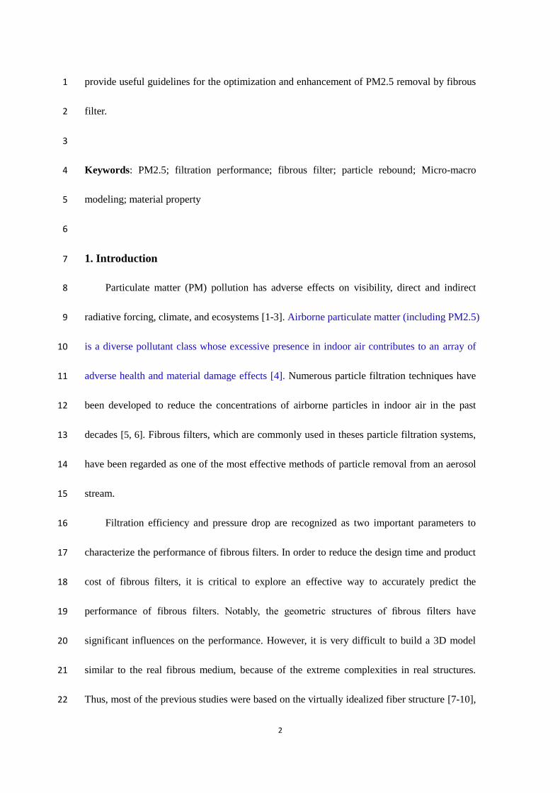
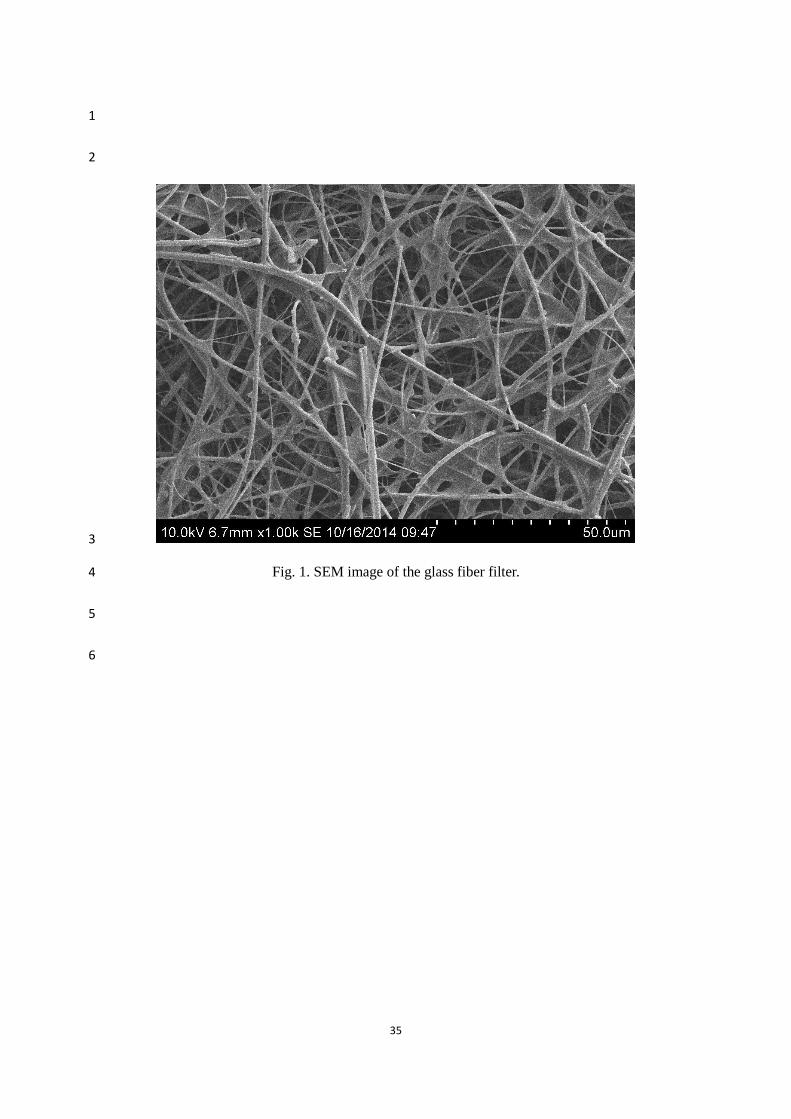
The structural morphology of the fiber filter is observed by SEM, as shown in Fig. 1. The 6

fiber diameter distribution of the filter is determined from the SEM image using the Image J 7

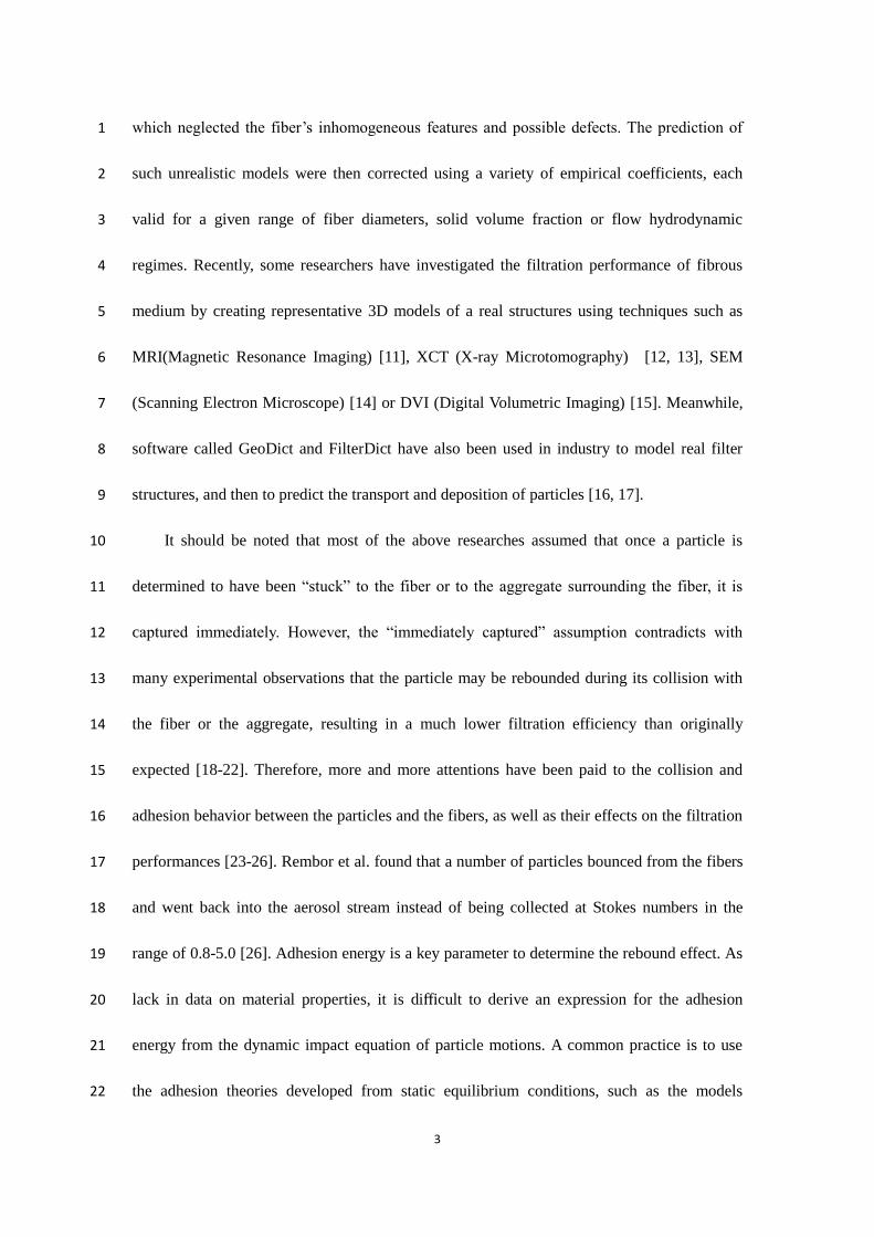
software (http://rsb.info.nih.gov/ij/). The bubble point (largest pore-size), mean pore-size, 8

smallest pore of the filter, as well as the pore size distribution are determined using a capillary 9

flow porometer (Porous Materials Inc., USA), see Fig. 2. Then the SVF (Solid Volume 10

Fraction) of the filter can be calculated. All the basic characteristics of the fiber filter are 11

expressed as mean ±standard deviation in Table 1. 12

13

Table 1 Basic characteristics for the investigated glass fiber filter. 14

Fig. 1. SEM image of the glass fiber filter. 15

Fig. 2. Morphological characteristics for fiber filter. (a) Fiber size distribution of the filter, (b) 16

Pore size distribution of the filter. 17

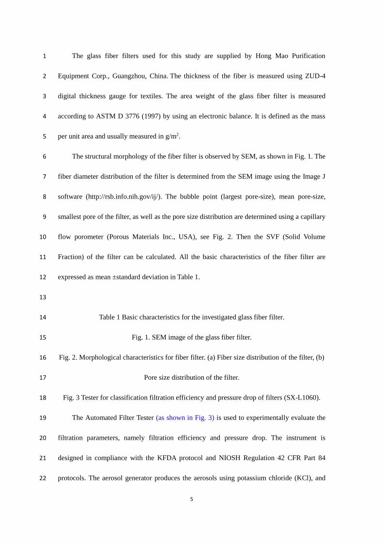
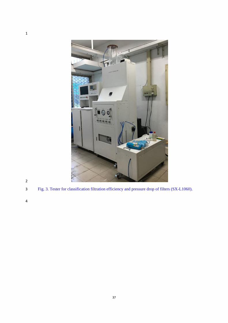
Fig. 3 Tester for classification filtration efficiency and pressure drop of filters (SX-L1060). 18

The Automated Filter Tester (as shown in Fig. 3) is used to experimentally evaluate the 19

filtration parameters, namely filtration efficiency and pressure drop. The instrument is 20

designed in compliance with the KFDA protocol and NIOSH Regulation 42 CFR Part 84 21

protocols. The aerosol generator produces the aerosols using potassium chloride (KCl), and 22

6

then dries and neutralizes them to ensure accurate results. The relative humidity is maintained 1

to be 30% during the experiments. Polydisperse aerosols, ranged from 0.015 μm to 0.80 μm 2

are pulled down through the filter by a vacuum pump. The targeted face velocities can be set 3

by adjusting the flow rates of the aerosol flow. Two solid-state laser-based light scattering 4

photometers measure the aerosol concentration, with one placed before and the other after the 5

filter. The photometer output signals are approximately proportional to the aerosol mass and 6

used to calculate the filter penetration P as 7

100(%)up

down C

CP (1) 8

where downC is the aerosol concentration downstream of the filter and

upC is the aerosol 9

concentration upstream of the filter. The filtration efficiency of the filter can then be 10

calculated as P1 . Filtration efficiencies for each particle size are measured 11

simultaneously by several sets of photometers. Pressure drop is measured at a given airflow 12

rate using a pressure gauge. The penetration and pressure drop are recorded at about 1-min 13

intervals throughout the test. For each filter under one test condition, the experiments are 14

performed five to ten times, and all data on penetration and pressure drop values are analyzed 15

using arithmetic mean values. 16

2.2 3D structure modeling 17

3D model of the investigated glass fiber filter is reconstructed from SEM images in the 18

following steps. 19

(1) The Gaussian blur (radius equal to three pixels) is applied to the original SEM image 20

to reduce the major pixel noise (see Fig. 4a and b). 21

(2) The average threshold level is applied for the grayscale SEM sample image to get the 22

7

upper fibers, resulting in a binary SEM image (see Fig. 4c). According to the study of 1

Ghasemi-Mobarakeh [31], a threshold of 0( ) / 255 is used to extract the outer layers of 2

the fiber. 0 and are the mean and standard deviation of the image matrix respectively. 3

(3) To keep the connectivity of the image, the binary SEM image is imported to Auto 4

CAD software and repair manually. Meanwhile the single black or white pixels representing 5

the minor noise are removed from the image. (see Fig. 4d) 6

(4) The centerline pixels of each fiber are calculated according to Zhang-Suen fast 7

parallel thinning algorithm [32]. The continuous centerline curves for each individual fiber 8

part are determined by the grouping of those centerline pixels having less than three 9

neighboring pixels. (see Fig. 4e and Fig. 4f) 10

(5) The 3D shape of each fiber is created by drawing cylinders along the centerline pixels. 11

Each centerline pixel point is firstly viewed as the bottom center of a cylinder. The height of 12

the cylinder is 1 pixel. Then the cylinder radius is increased till at least one white pixel 13

(representing the fiber surface) is reached [14]. Resulting 3D binary image is considered to be 14

the fiber filter of single layer. (see Fig. 4g). 15

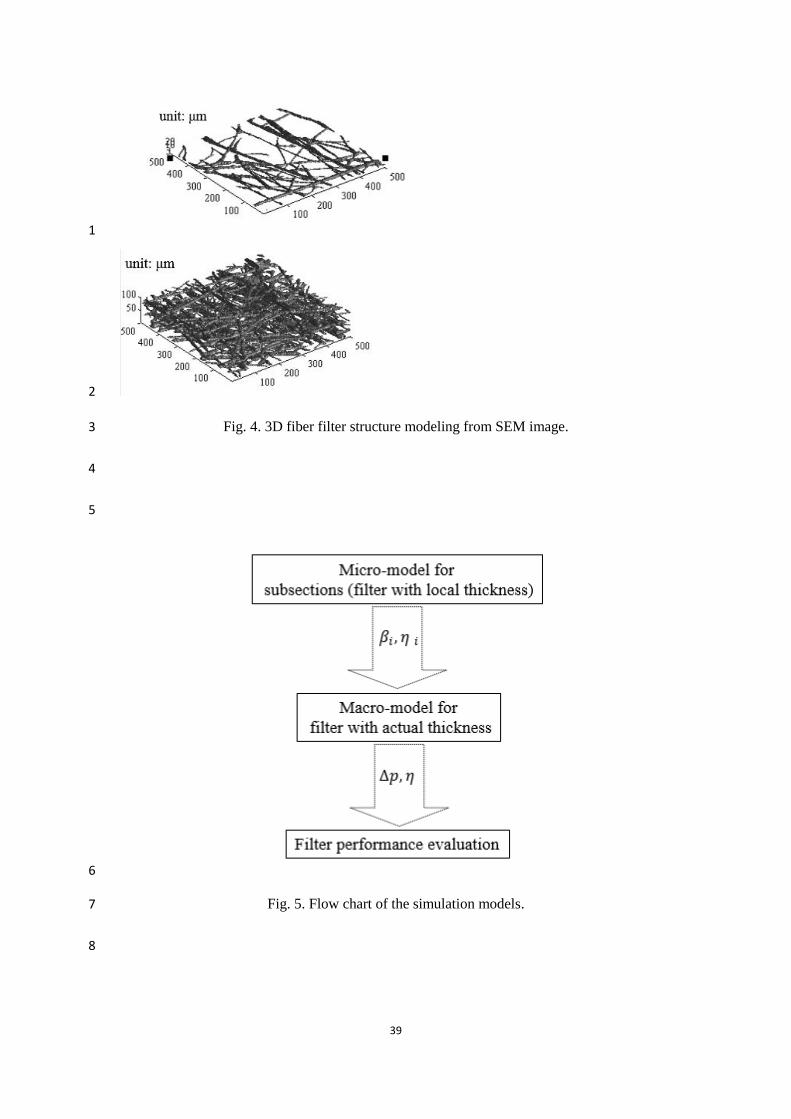
(6) The final 3D filter model of the filter is built up as the stack of the N model layers. 16

It is assumed that the structures of the inner layers of the filter are similar to that of the outer 17

layer. Thus, 3D models of several outer layers at different positions are constructed for 18

stacking. The reconstructed fibrous filter should satisfy the following two principles. (1) The 19

thickness of the reconstructed filter should equal or close to the real filter thickness. (2) The 20

calculated mass area of the reconstructed filter should close to the measured values of the real 21

filter. The least square method is used for searching the optimal value, and the layer number 22

8

N is determined by the following equation[14] : 1

minimum|(|1

mci

N

i

mm (2) 2

where cim is the calculated mass area of the i th model layer and mm is the measured mass 3

area of N layers. Fig. 4h shows a 3D filter model with thickness of 10 μm. 4

(7) Software Mimics (http://biomedical.materialise.com/mimics) is used to convert the 5

3D binary images to the filter entity for the further mesh generation. 6

7

Fig. 4. 3D fiber filter structure modeling from SEM image. 8

9

3 Micro-scale modeling of filter with local thickness 10

The actual fiber filter investigated is very thick ( h =200 μm), thus it is difficult to 11

simulate the actual thickness with acceptable computational load, while considering its 12

microscopic flow structure at the same time. In this study, a multi-scale simulation method is 13

used to predict the filtration efficiency and the pressure drop of the fibrous filter. Firstly, the 14

filter is divided into several subsections along its thickness, each with a local thickness of 15

ih =10 μm. Then the micro-scale model of a single subsection filter is set up and simulated. 16

Finally, using the micro-scale simulated results, the model of the filter with actual thickness is 17

established, in which the fiber filter is regarded as a homogeneous porous medium with 18

constant viscous resistance coefficient, which is a mature methodology in common CFD 19

software. The flow chart of the models is presented in Fig. 5. 20

21

Fig. 5. Flow chart of the simulation models. 22

9

1

In this section, the steady flow equations and the numerical scheme for simulating the 2

gas-solid flow in the filter with a local thickness (the subsection) are presented firstly. Then 3

the slip velocity boundary conditions, as well as mesh independence and computation domain 4

independence tests are studied. The emphasis will be laid on the modeling of particle-fiber 5

collisions and rebound. The results are used to draw the resistance coefficients for 6

macro-scale modeling of the whole filter. 7

3.1 Governing equations for air flow 8

For the range of fiber size and flow conditions consider in this study, the Reynolds 9

number is smaller than unity. Thus the air flow through the fibrous medium is assumed to be 10

laminar, incompressible and at a steady state. The finite volume method [33] implemented in 11

the Ansys 13.0 code is used to solve the air flow field. The governing equations: continuity 12

and conservation of linear momentum are as follows. It should be noted that the influence of 13

particles on the air flow is neglected. 14

0 UDt

D

(3) 15

)(3

4)( UUp

Dt

DU (4) 16

where, , U , and p are the density, velocity, dynamic viscosity and pressure of the air 17

respectively. 18

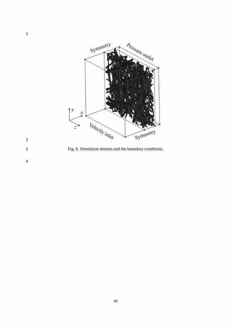
3.2 Boundary conditions 19

The computational region as well as the boundary conditions considered for the 20

simulations are shown in Fig. 6. At the inlet, the Dirichlet boundary condition is employed to 21

specify the gas velocity to the fibrous filter. The atmospheric pressure is imposed at the outlet. 22

10

There is to be noted that, uniform air flow inlet boundary condition has been placed at a 1

distance of 20fd upstream of the filter, and outlet boundary conditions at a distance of 5

fd 2

downstream of the filter [34] to avoid the interruption from the regions where strong velocity 3

and pressure gradients are expected. A symmetry boundary condition is used for the sides of 4

the computational region. Such a boundary condition will not affect the simulation results, as 5

the flow is dominantly in the through-plane direction, and lateral flows are relatively weak. 6

7

Fig. 6. Simulation domain and the boundary conditions. 8

9

For the air flow on the fiber surfaces, a slip boundary condition is adopted. Because 10

under the air thermal condition and the fiber diameters considered in this study, the fiber 11

Knudsen number, f

f

20.001Kn

d

( is the mean free path of the air molecules and it is 12

about 60 nm). This means that the slip flow prevails insider the fibrous filter in this study. To 13

add this feature to the Ansys13.0 code, a UDF (User Defined Function) that considering the 14

slip velocity at the fiber surfaces is developed. The wall shear stress is defined using the 15

Maxwell first order model [35] 16

w

v

vw |

2

n

UU

(5) 17

where, WU is the air velocity at the wall,

v is the tangential momentum accommodation 18

coefficient. 19

3.3 Particle flow and capture 20

Once the particle-free flow field is obtained, the particulates, modeled by rigid spheres of 21

uniform density P =3000 kg/m3 are then introduced into the domain. Using the Lagrangian 22

11

method, the force balance on a particle is integrated to obtain the particle position with time. 1

The dominant forces acting on the particles without considering collision are the drag force 2

exerted by the air flow and the Brownian force: 3

bipiid

pi

p )( FUUFdt

dUm (6) 4

where, p p, m U and pd are the particle mass, velocity and diameter. U is the air flow 5

velocity. dF and

biF are the amplitudes of the drag (for p pRe /Ud ) and Brownian 6

force. They are given as 7

cp

2p

d

18

CdF

(7) 8

and 9

)(

218

cp2p

ibi

Sct

U

CdF

(8) 10

TC

UdSc

Bc

p3

(9) 11

where, f1.1/

c f1 (1.257 0.4 )Kn

C Kn e

is an empirical correction factor called 12

Cunningham slip correction factor. i are zero-mean, unit-variance independent Gaussian 13

random numbers. T is the absolute temperature of the air, and B is the Boltzmann 14

constant. The amplitudes of the Brownian force components are evaluated at each time step. 15

The particle trajectory calculation implemented in Ansys13.0 code is referenced by Qunis and 16

Ahmadi [36]. 17

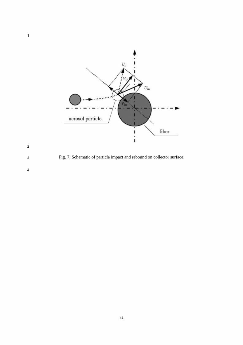
Now the collision is considered. To take into account the interception capture 18

mechanism, a C++ subroutine that works in Ansys13.0 enviroment is developed. During each 19

trajectory tracking step, the distances between the particles’ centers and the fiber surfaces are 20

monitored. Once the distance is smaller than the particle radius, the particle is regarded to be 21

12

collided with the fiber. As shown in Fig. 7, the model of the particle-fiber collision 1

implemented here is based on a suggestion of Dahneke [37] and it is consisted of an energy 2

balance around the particle-fiber collision as follow 3

rp,2

inp,ink,rk, )( EeEEE (10) 4

where k,inE and p,inE are the kinetic energy and potential energy before collision 5

respectively. k,rE and p,rE are the kinetic energy and potential energy after collision 6

respectively. e is the coefficient of restitution. The prerequisites of the adhesion of a particle 7

is that the particle is not able to leave the fiber after the collision, thus k,rE =0. Assuming that 8

p,in p,r wE E E , it yields a critical particle velocity 9

2/1

2p

2w

cr ])1(2

[em

eEU

(11) 10

Thus, when in crU U , then the particle would be rebounded, and the rebounded particle 11

velocity satisfies r inU U e . Otherwise, it would be captured by the fiber. 12

The coefficient of restitution e can be calculated by following formula [29] 13

1)7.1exp(0 ee (12) 14

where, 0e is the value when collision velocity in normal condition approaching to zero and it 15

can be chosen as 0e =0.965 is an elastic parameter associated with fiber and particle 16

materials, and it can be calculated by 17

5/2

fp

f5/3

f

in

10/1

f

pf

p

5/2)()(

)1(

1

3

2

kk

kU

d

dd

d

(13) 18

p)f,( 1

iE

ki

ii

(14) 19

where, and E are the Poisson 's ratio and the Young's modulus of the fiber or particle. 20

13

1

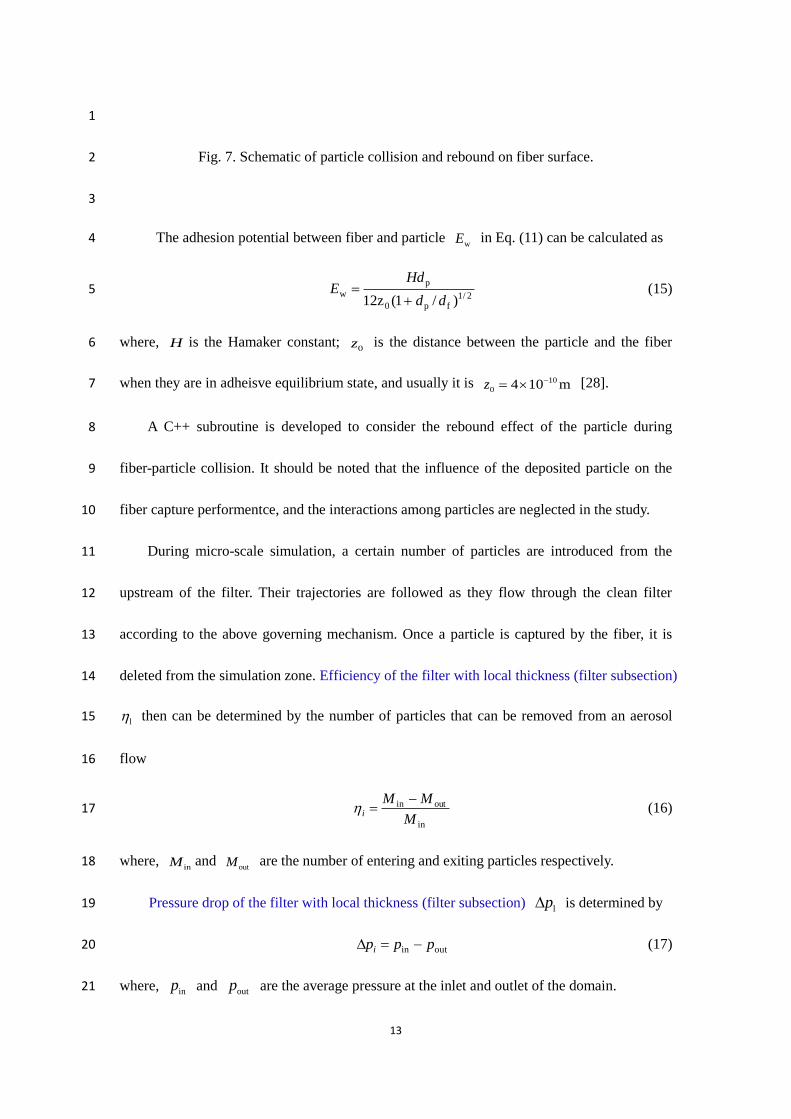
Fig. 7. Schematic of particle collision and rebound on fiber surface. 2

3

The adhesion potential between fiber and particle wE in Eq. (11) can be calculated as 4

2/1

fp0

p

w)/1(12z dd

HdE

(15) 5

where, H is the Hamaker constant; 0z is the distance between the particle and the fiber 6

when they are in adheisve equilibrium state, and usually it is 10

0 4 10 mz [28]. 7

A C++ subroutine is developed to consider the rebound effect of the particle during 8

fiber-particle collision. It should be noted that the influence of the deposited particle on the 9

fiber capture performentce, and the interactions among particles are neglected in the study. 10

During micro-scale simulation, a certain number of particles are introduced from the 11

upstream of the filter. Their trajectories are followed as they flow through the clean filter 12

according to the above governing mechanism. Once a particle is captured by the fiber, it is 13

deleted from the simulation zone. Efficiency of the filter with local thickness (filter subsection) 14

l then can be determined by the number of particles that can be removed from an aerosol 15

flow 16

in

outin

M

MMi

(16) 17

where, inM and

outM are the number of entering and exiting particles respectively. 18

Pressure drop of the filter with local thickness (filter subsection) lp is determined by 19

outin pppi (17) 20

where, inp and outp are the average pressure at the inlet and outlet of the domain. 21

14

3.4 Mesh independence test 1

Software ICEM is used for meshing the fibrous filter entity. The imported geometries are 2

meshed using tetrahedral elements, refined close to the fiber surfaces. In an irregular structure, 3

such as fiber filter, there are regions where fiber-to-fiber distance is very small such as at the 4

crossovers, and regions where fibers are relatively far from each other. The grid size required 5

to mesh the gap between two fibers around their crossover point is often too small. The 6

computational grid used for CFD simulations needs to be fine enough to solve the flow field 7

in the narrow gaps, and at the same time coarse enough to cover the whole domain without 8

requiring too much computational power. 9

To ensure that the simulation results are independent of the number of grid points, one 10

filter with local thickness of 10 μm is considered and meshed with different mesh densities. 11

This is done by adjusting the grid interval size in such a way that resulting in 9, 16, 25, 36, 49 12

64, 81 and 100 grids on the circular cross-section of the fibers. The results of the mesh 13

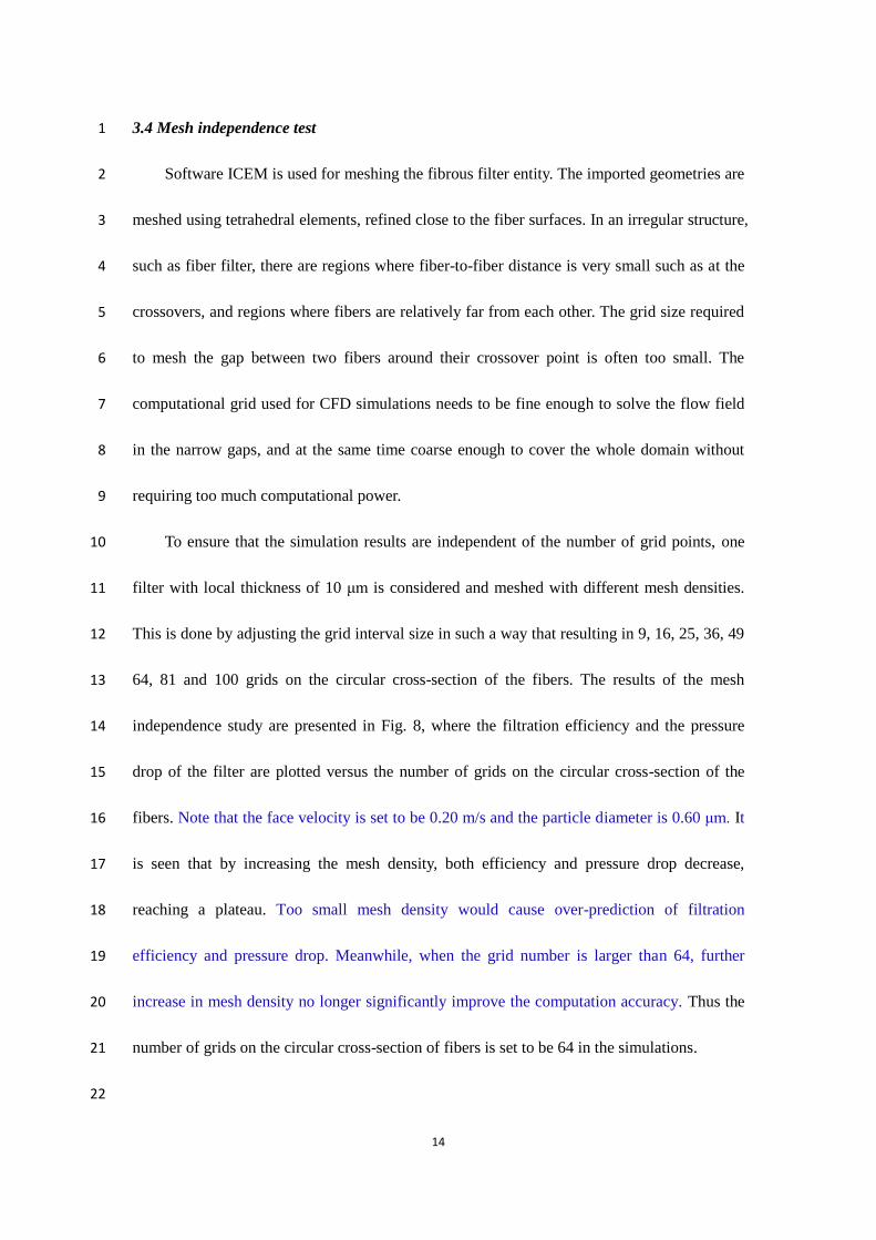
independence study are presented in Fig. 8, where the filtration efficiency and the pressure 14

drop of the filter are plotted versus the number of grids on the circular cross-section of the 15

fibers. Note that the face velocity is set to be 0.20 m/s and the particle diameter is 0.60 μm. It 16

is seen that by increasing the mesh density, both efficiency and pressure drop decrease, 17

reaching a plateau. Too small mesh density would cause over-prediction of filtration 18

efficiency and pressure drop. Meanwhile, when the grid number is larger than 64, further 19

increase in mesh density no longer significantly improve the computation accuracy. Thus the 20

number of grids on the circular cross-section of fibers is set to be 64 in the simulations. 21

22

15

Fig. 8. Influence of mesh density on efficiency and pressure drop calculations. 1

2

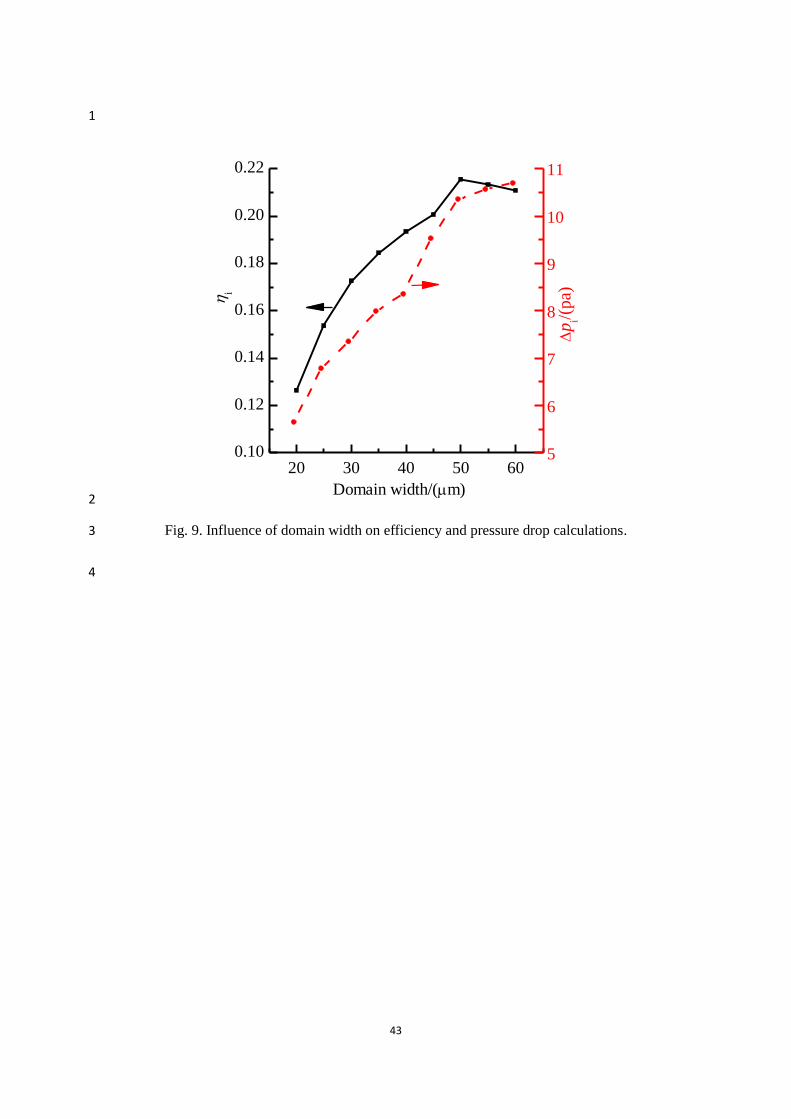
3.5 Computation domain independence test 3

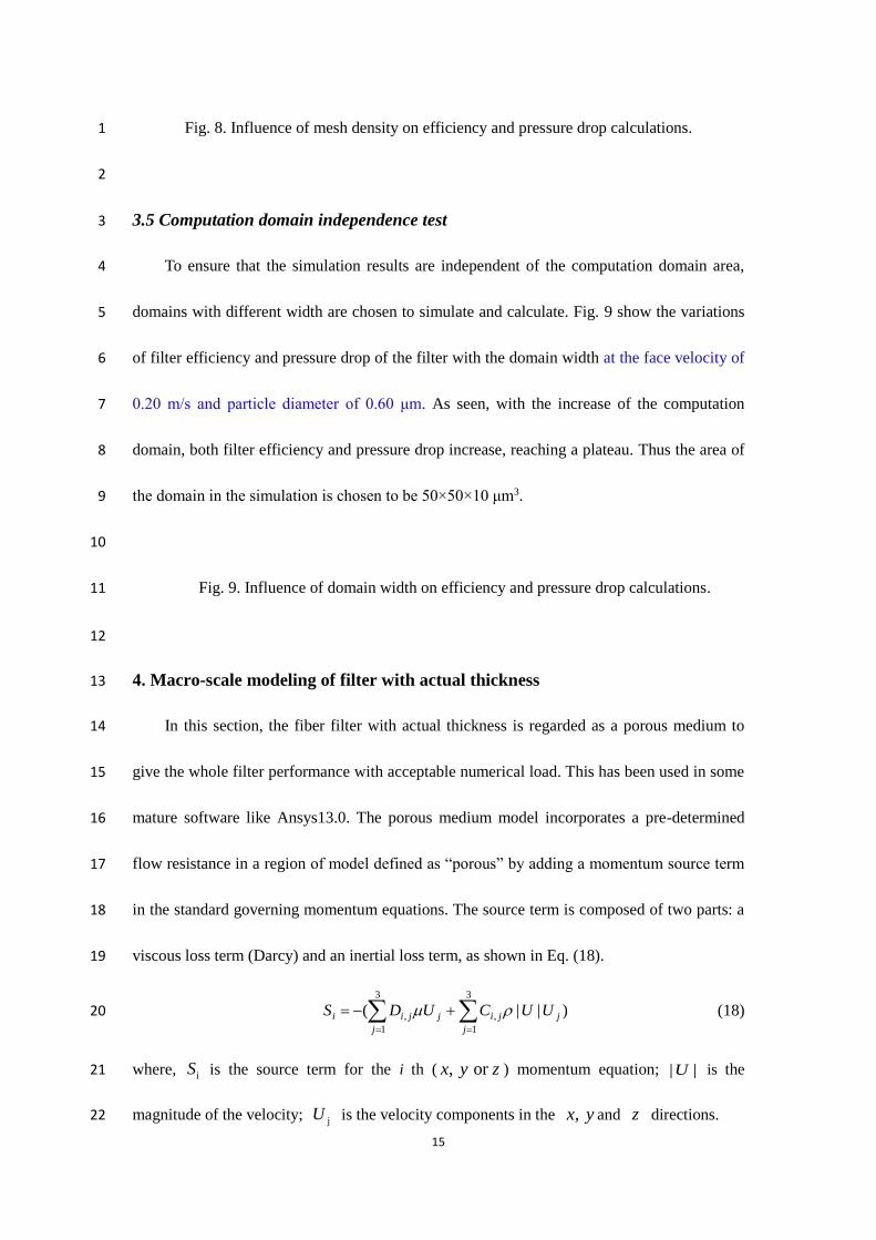
To ensure that the simulation results are independent of the computation domain area, 4

domains with different width are chosen to simulate and calculate. Fig. 9 show the variations 5

of filter efficiency and pressure drop of the filter with the domain width at the face velocity of 6

0.20 m/s and particle diameter of 0.60 μm. As seen, with the increase of the computation 7

domain, both filter efficiency and pressure drop increase, reaching a plateau. Thus the area of 8

the domain in the simulation is chosen to be 50×50×10 μm3. 9

10

Fig. 9. Influence of domain width on efficiency and pressure drop calculations. 11

12

4. Macro-scale modeling of filter with actual thickness 13

In this section, the fiber filter with actual thickness is regarded as a porous medium to 14

give the whole filter performance with acceptable numerical load. This has been used in some 15

mature software like Ansys13.0. The porous medium model incorporates a pre-determined 16

flow resistance in a region of model defined as “porous” by adding a momentum source term 17

in the standard governing momentum equations. The source term is composed of two parts: a 18

viscous loss term (Darcy) and an inertial loss term, as shown in Eq. (18). 19

)||(3

1

3

1

,, j

j j

jijjii UUCUDS

(18) 20

where, iS is the source term for the i th ( , or x y z ) momentum equation; | |U is the 21

magnitude of the velocity; jU is the velocity components in the , x y and z directions. 22

16

For laminar flow through a filter in this study, the pressure drop is typically proportional 1

to velocity and the porous medium model then reduces to Darcy’s Law: 2

Uh

p

(19) 3

where, is the viscous resistance coefficient and also the entries in the matrix D in Eq. 4

(18). Also according to Darcy’s Law, the viscous resistance coefficients of each filter 5

subsection (totally 20 subsections) at different face velocities can be calculated using the 6

micro-scale simulation result as Uhp lll / . Then through macro-scale simulation, the 7

pressure drop of an actual filter can be obtained. 8

The efficiency of the filter with actual thickness is calculated by 9

t

i

i

1

l )1(1 (20) 10

where t is the number of the filter subsections, il represents the capture efficiency of ith 11

filter subsection. 12

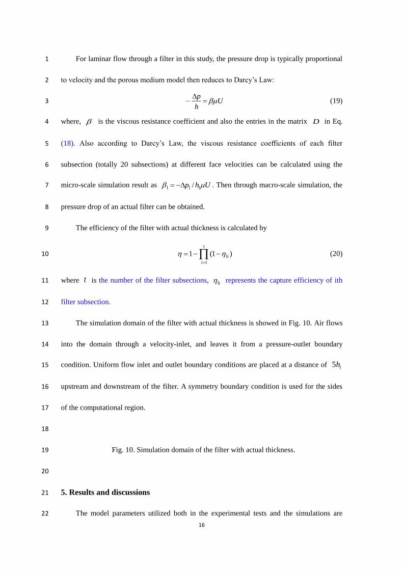
The simulation domain of the filter with actual thickness is showed in Fig. 10. Air flows 13

into the domain through a velocity-inlet, and leaves it from a pressure-outlet boundary 14

condition. Uniform flow inlet and outlet boundary conditions are placed at a distance of l5h 15

upstream and downstream of the filter. A symmetry boundary condition is used for the sides 16

of the computational region. 17

18

Fig. 10. Simulation domain of the filter with actual thickness. 19

20

5. Results and discussions 21

The model parameters utilized both in the experimental tests and the simulations are 22

17

listed in Table 2. Note that the parameter values of the particles and fibers used in the 1

simulation are assumed to be in the dry state. The operating conditions in experiments are 2

expressed as arithmetic mean ±standard deviation. Micro-scale model simulation is conducted 3

firstly to get the local viscous resistance, as well as the performance of the filter with local 4

thickness. Note that the inlet velocity and particle concentration of the first subsection are 5

specified according to the operating conditions, while, that of the other subsections are 6

specified to be equal to the outlet velocities and particle concentrations of the upper 7

subsections. Then the macro-scale model is used to get the performance of the fiber filter with 8

actual thickness. The results are compared with that calculated from available correlations in 9

literature [38] or the experimental data. The rebound effect during fiber filtration, as well as 10

the influence of the particle size, face velocity on the filtration performance are analyzed and 11

discussed. Note that the experimental tests are repeated five to ten times in order to get 12

average values and standard deviations. 13

14

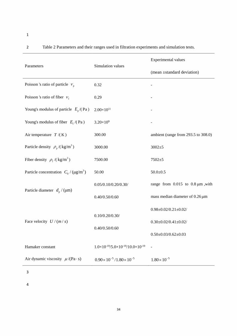
Table 2 Parameters and their ranges used in filtration experiments and simulation tests. 15

16

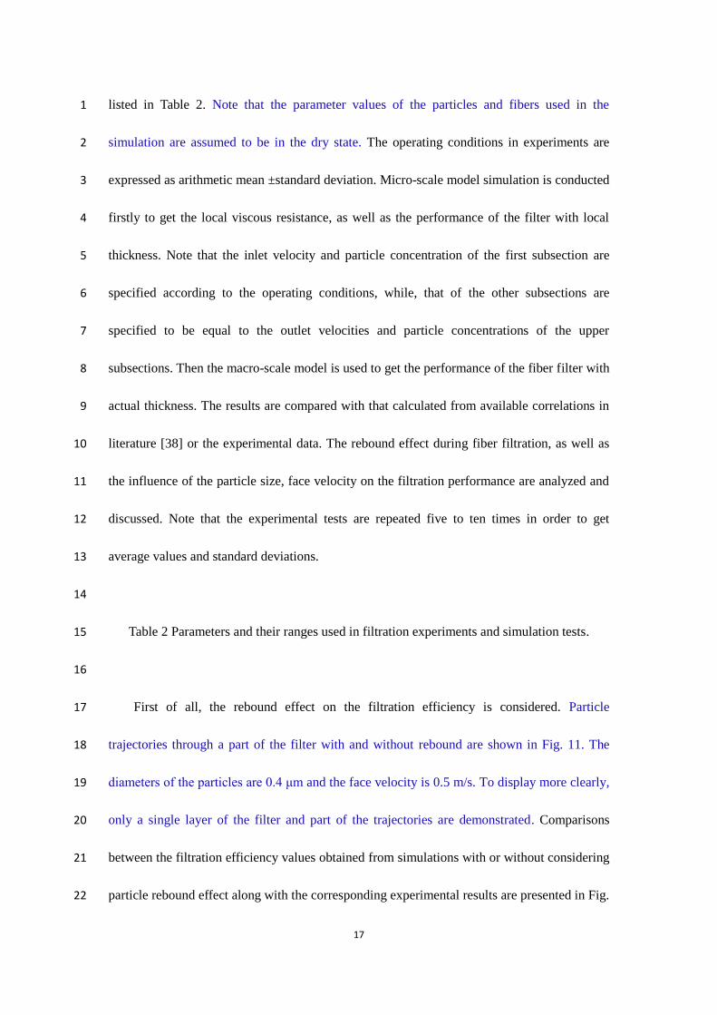
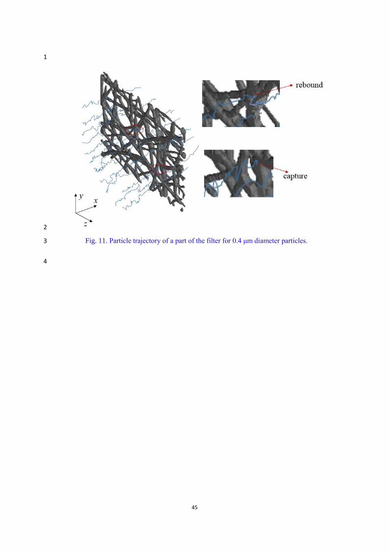
First of all, the rebound effect on the filtration efficiency is considered. Particle 17

trajectories through a part of the filter with and without rebound are shown in Fig. 11. The 18

diameters of the particles are 0.4 μm and the face velocity is 0.5 m/s. To display more clearly, 19

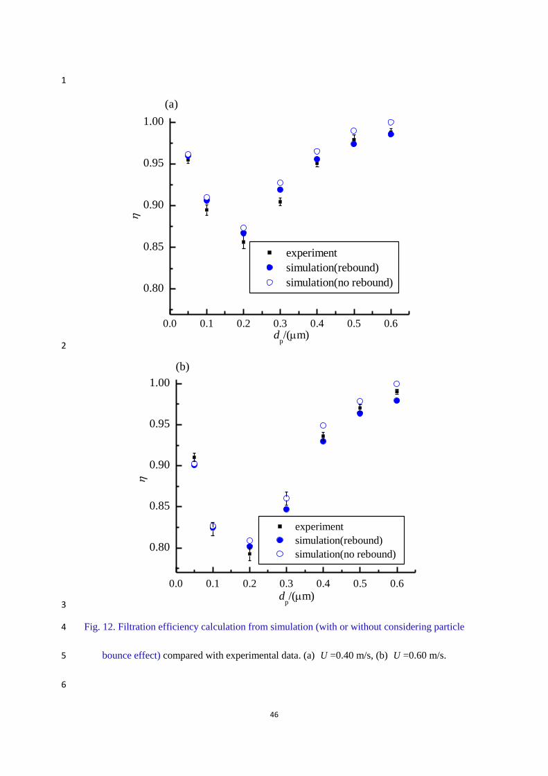
only a single layer of the filter and part of the trajectories are demonstrated. Comparisons 20

between the filtration efficiency values obtained from simulations with or without considering 21

particle rebound effect along with the corresponding experimental results are presented in Fig. 22

18

12. It can be seen that the simulation results considering the particle rebound effect are 1

generally in better agreement with the experimental data than that without considering 2

rebound effect. Additionally, it can be found that the difference between the two simulation 3

model results become larger gradually with the increase in the particle size, which implies that 4

the particle rebound effect is more significant when the particle diameter is large. When the 5

particle size is very small (i.e. μm 3.0p d ), the rebound effect can be negligible. It is seen in 6

Fig. 12 that the effects of face velocity on filtration efficiency decrease when the particle size 7

is larger than 0.5 µm. This is because when the particle diameter is 0.5 µm, the filtration 8

efficiency of the filter with actual thickness are already as high as 97%. Particles with 9

diameter larger than 0.5 µm do have higher efficiency, but the increment is not as significant 10

as that from 0.4 µm to 0.5 µm. 11

12

Fig. 11. Particle trajectory of a part of the filter for 0.4 μm diameter particles. 13

Fig. 12. Filtration efficiency calculation from simulation (with or without considering particle 14

rebound effect) compared with experimental data. (a) U =0.40 m/s, (b) U =0. 60 m/s. 15

16

Increasing the face velocity enhances the particle rebound effect to some extent. A 17

comparison example for face velocities of 0.40 m/s and 0.60 m/s can be seen in Fig. 12(a) 18

and Fig. 12(b). Because when the face velocity increases, the opportunity is higher for the 19

collision velocity of the particle inU to be larger than the critical velocity crU . Thus the 20

particle is more easily to rebound. 21

The influence of Hamaker constant on the rebound effect is investigated at the different 22

19

Stokes number (St). Note that the St is changed by changing face velocity and gas viscosity. 1

' is the ratio of filtration efficiency considering rebound effect to that without considering 2

rebound effect. As shown in Fig. 13, when St is small, the filtration efficiency values obtained 3

from simulations considering particle rebound effect are very close to that without 4

considering rebound effect. So it is not necessary to consider the particle rebound effect at 5

low Stokes numbers. When St is large, the rebound effect becomes more significant, and with 6

the increase of Hamaker constant, the filtration efficiency ratio ' increases. Because the 7

Hamaker constant is a measure of the adhesion force between particles and fibers. The larger 8

the Hamaker constant is, the larger the adhesion force is. Therefore, larger Hamaker constants 9

lead to weak rebound effect and high filtration efficiency. Further more, compared with the 10

results from literature [26], it is seen that the influence of particle rebound effect on filtration 11

efficiency is much weaker for an actual filter than for a single fiber. Because for an actual 12

filter, the rebound particles may collide with fiber several times and be captured later. 13

14

Fig. 13. The influence of Hamaker constant on the particle rebound and filtration efficiency 15

16

In the second step, the effect of face velocity, particle diameter on the filter performance 17

are investigated by the proposed simulation approach. Apart from the experimental data, some 18

empirical correlations are also used to verify the simulation results. 19

The empirical correlations for filtration efficiency used in this study is based on 20

Kuwabara’s cell model [39]. If the flow pattern and web structure of the fiber filter are known, 21

the filter efficiency , can be calculated from single fiber efficiency as [38] 22

20

)4

exp(1f

sg

d

h

(21) 1

The total single fiber efficiency sg is resulted from the combination of four basic 2

filtration mechanisms: interception R , inertial impaction I , gravitational settling (small 3

enough to be neglected here) and Brownian diffusion d . The calculation formulas used in 4

this study are listed below [38] 5

)1)(1)(1(1 dIRsg (22) 6

22R )1(

2)

21()

1

1(1)1ln(2[

2

1R

RR

Ku

R

(23) 7

2I

2

)(

Ku

JSt (24) 8

f

cp2p

18St

d

UCd

(25) 9

8.2262.0 5.27)286.29( RRJ (26) 10

3/23/1d )

1(6.1

PeKu

(27) 11

where 4/4

3)

2ln( 2

Ku is the Kuwabara’s hydrodynamic coefficient and 12

p f/R d d is the particle to fiber diameter ratio. f /Pe Ud D is the Peclet number. 13

B c

P3

C TD

d

is the diffusion coefficient, and

231.38 10B m2·kg·s-2·K-1 is the 14

Boltzmann constant. 15

The pressure drop of the filter is a function of face velocity, filter thickness, air dynamic 16

viscosity, fiber diameter and dimensionless pressure drop ( )f as [40] 17

2f

)(d

hUfp

(28) 18

The predictions obtained via the empirical correlation of Ogorodnikov obtained for slip and 19

transition regime is [41] 20

21

4

f )1(15.1ln5.05.0

16)(

Knf (29) 1

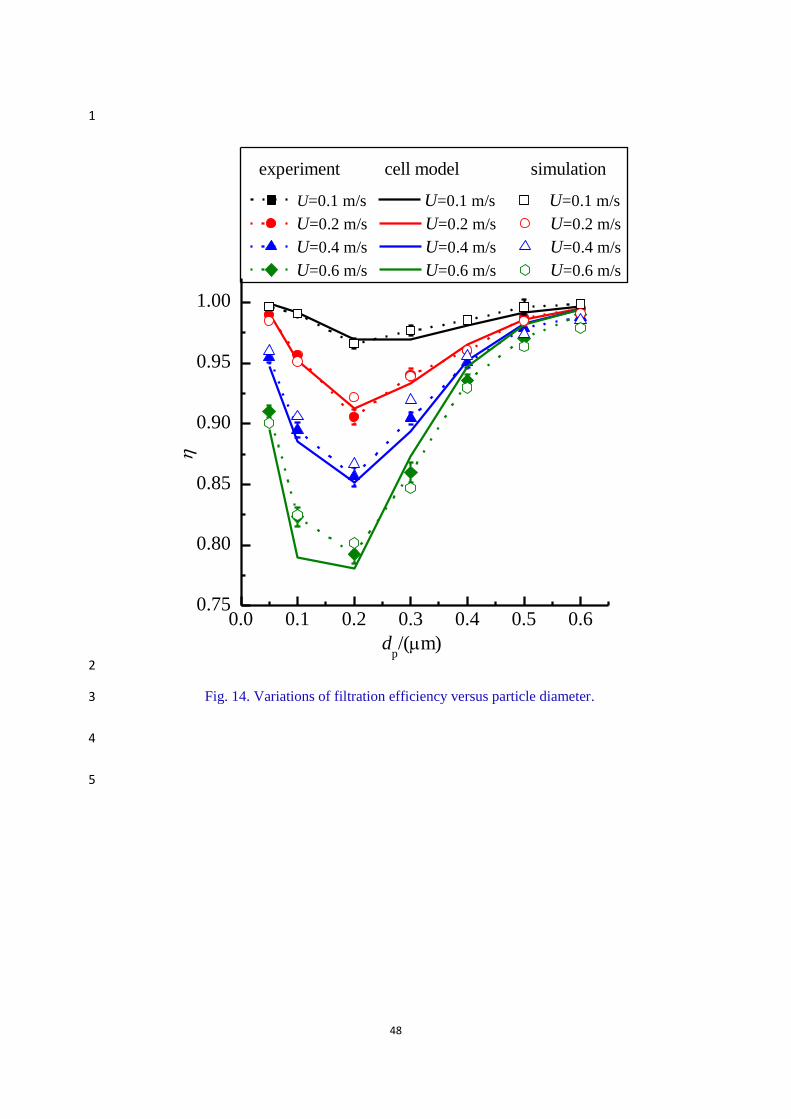
Fig. 14 shows the filtration efficiency of the filter with actual thickness versus particle 2

diameter along with the Kuwabara’s cell model and the experimental results. It can be seen 3

that the filter collection efficiency decreases at first and then increases subsequently by 4

increasing the particle size in the range of 0.05-0.6 μm, with the minimum filtration efficiency 5

at particle diameter of 0.2 μm. The filtration efficiency predicted by the simulations follows a 6

trend similar to that of the cell model of Eq. (21) and the experimental results. As an 7

important indicator for interception mechanism, the intercept coefficient ( R ) is ranged from 8

0.05 to 0.6 in this study. When R is large, the Stokes number is proportional to the square of 9

the particle size. It is clarified that the inertia is strengthened with increasing particle size 10

which makes the filtration efficiency increase. When R is small, Brownian force, rather 11

than the air flow field, dominantly influences the particle trajectory, thus the filtration 12

efficiency decreases with the increasing in particle diameter. The deviations of the model 13

filtration efficiency for the large particle sizes ( 0.3 μm) are mainly due to the particle 14

trajectory calculations, because the air flow plays the dominant role for the large particles and 15

their impacts on the air flow are neglected in the model. The deviations at the small particle 16

size range ( 0.3 μm) can be caused by the van der Waals force which is difficult to fully take 17

into account in the model and the possible existence of electrostatic force in the experiments. 18

The deviation is the largest for particle sizes of 0.3 μm, and it may be due to the combined 19

effects of the above two factors. 20

Fig. 14. Variations of filtration efficiency versus particle diameter. 21

22

22

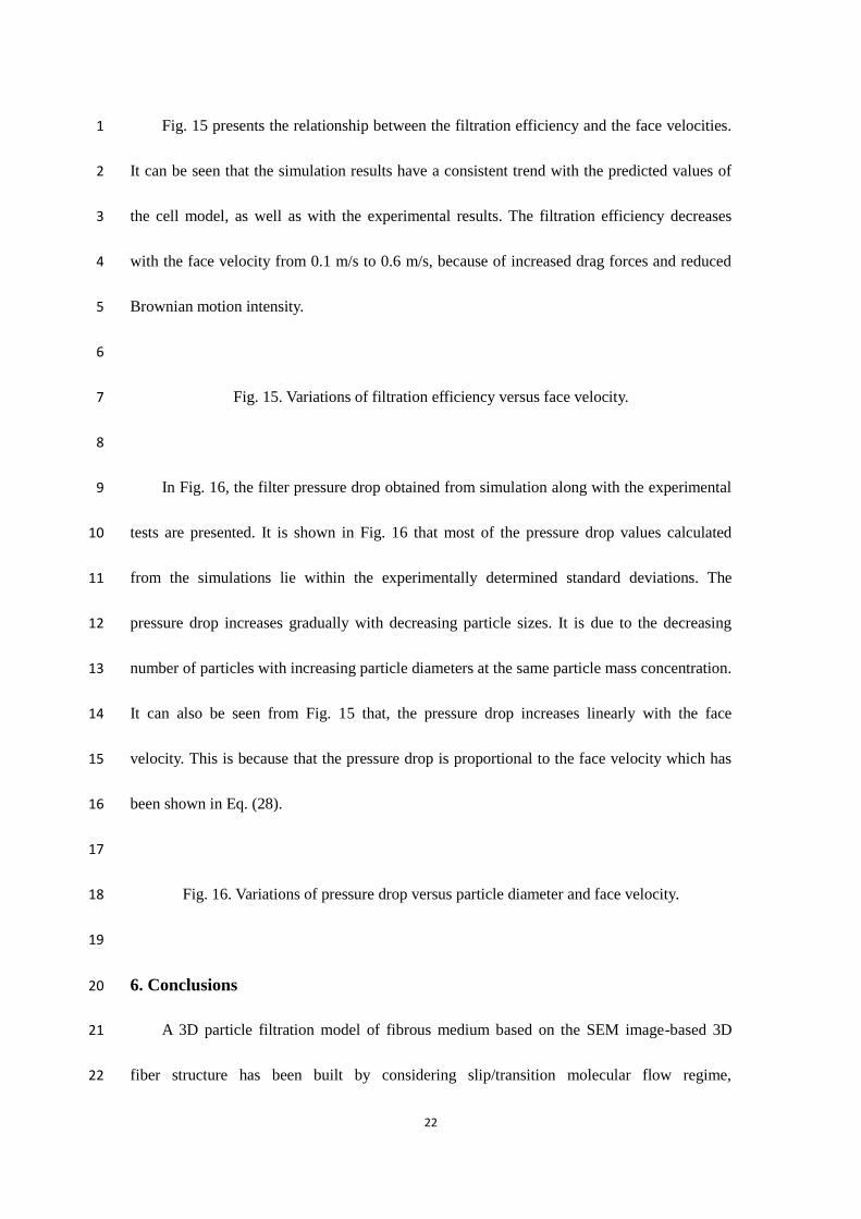
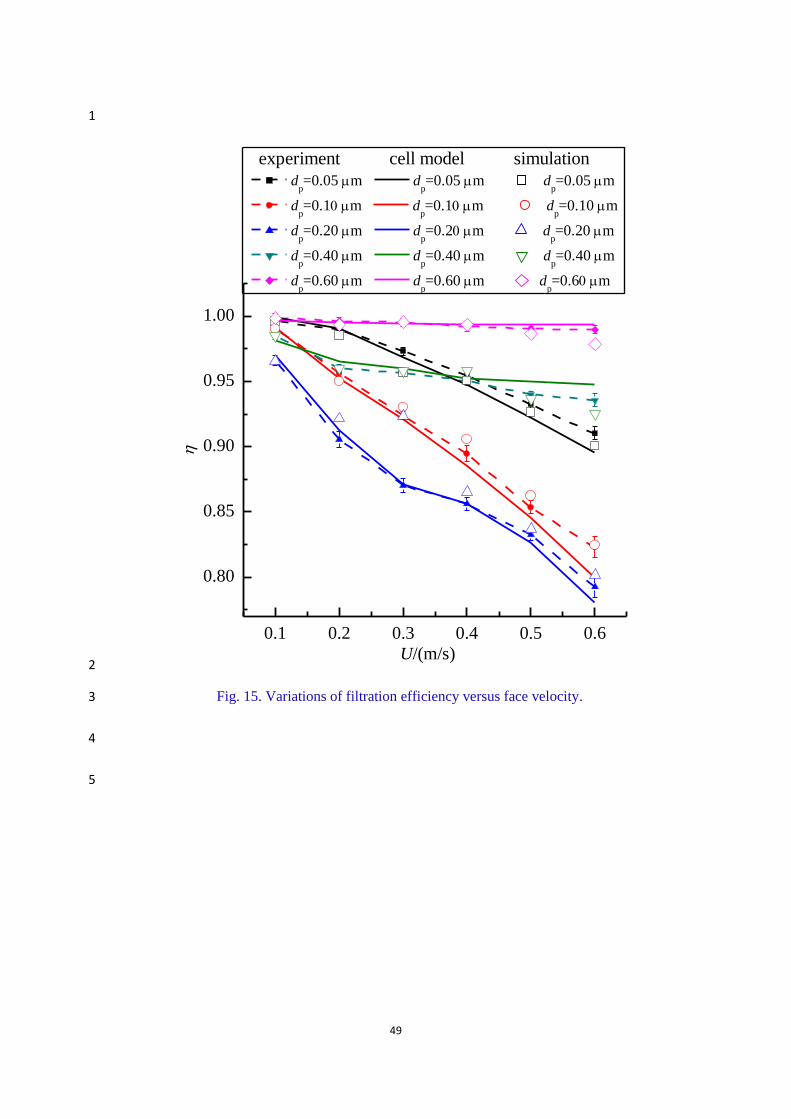
Fig. 15 presents the relationship between the filtration efficiency and the face velocities. 1

It can be seen that the simulation results have a consistent trend with the predicted values of 2

the cell model, as well as with the experimental results. The filtration efficiency decreases 3

with the face velocity from 0.1 m/s to 0.6 m/s, because of increased drag forces and reduced 4

Brownian motion intensity. 5

6

Fig. 15. Variations of filtration efficiency versus face velocity. 7

8

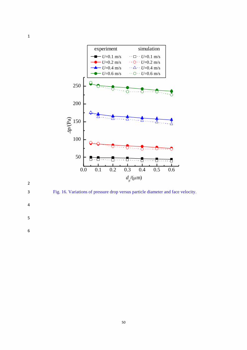
In Fig. 16, the filter pressure drop obtained from simulation along with the experimental 9

tests are presented. It is shown in Fig. 16 that most of the pressure drop values calculated 10

from the simulations lie within the experimentally determined standard deviations. The 11

pressure drop increases gradually with decreasing particle sizes. It is due to the decreasing 12

number of particles with increasing particle diameters at the same particle mass concentration. 13

It can also be seen from Fig. 15 that, the pressure drop increases linearly with the face 14

velocity. This is because that the pressure drop is proportional to the face velocity which has 15

been shown in Eq. (28). 16

17

Fig. 16. Variations of pressure drop versus particle diameter and face velocity. 18

19

6. Conclusions 20

A 3D particle filtration model of fibrous medium based on the SEM image-based 3D 21

fiber structure has been built by considering slip/transition molecular flow regime, 22

23

particle-fiber rebound effect and Brownian diffusion effect. The predicted filtration efficiency 1

and pressure drop values have been compared with experimental data and available empirical 2

correlations. It is found that the simulation results are in good agreement with that obtained 3

from experiments and correlations. 4

The effects of different factors such as air velocity, particle diameter and material 5

property (Hamaker constant) have been investigated for the real filters. It is revealed that the 6

particle rebound effect becomes significant at high Stokes numbers (St>1.0), whereas its 7

impact on filtration efficiency is not as significant as that for a single fiber. The rebound effect 8

increases with decreasing Hamaker constant, a measure of adhesion force. The variations of 9

predicted performance with operating parameters are well in consistency with the 10

experimental results. It is proved that the proposed modeling tool in this work will help to 11

predict the filtration efficiency and pressure drop of clean real fibrous medium, and to provide 12

useful guidelines for their optimization and enhancement. 13

14

Acknowledgments 15

The current work is supported by National Science Fund for Distinguished Young 16

Scholars of China (No.51425601); the Research Team Fund of Natural Science Foundation of 17

Guangdong Province (No.2014A030312009). It is also supported by Natural Science 18

Foundation of China, No. 51376064; National Science Fund for Young Scholars of China (No. 19

51506058) and Postdoctoral Science Foundation of China (No.2015M570711). 20

21

24

Nomenclature 1

0C particle concentration, μg/m3 2

cC Cunningham slip correction factor 3

D diffusion coefficient, m2·s-1 4

d diameter, μm 5

pord pore diameter of filter, μm 6

e restitution coefficient 7

E Young's modulus, Pa 8

0e restitution coefficient constant 9

kE kinetic energy, J 10

pE potential energy, J 11

wE adhesion potential between fiber and particle, J 12

bF Brownian force, N 13

dF drag force, N 14

h thickness of entire filter, μm 15

fh thickness of filter subsection, μm 16

H Hamaker constant 17

fKn fiber Knudsen number 18

Ku Kuwabara’s hydrodynamic coefficient 19

m mass, g 20

sm mass area, g/m2 21

cim calculated mass of the i th layer, g 22

25

mm measured mass of N layers, g 1

M particle number 2

N number of filter layer 3

p pressure, Pa 4

P penetration, % 5

Pe Peclet number 6

R particle to fiber diameter ratio 7

pRe particle Reynold number 8

Sc Schmidt number 9

St Stokes number 10

t number of filter layers 11

T absolute temperature of the air, K 12

U air velocity, m/s 13

crU critical rebound velocity, m/s 14

PU particle velocity, m/s 15

wU air velocity at the wall, m/s 16

Poisson 's ratio 17

0z distance between particle and fiber in adheisve equilibrium state, m 18

Greek letters 19

solid volume fraction, % 20

viscous resistance coefficient 21

t time step, s 22

26

p pressure drop of filter, Pa 1

lp pressure drop of filter subsection, Pa 2

elastic coefficient during collision 3

i Gaussian random number 4

filtration efficiency, % 5

' filration efficiency ratio, % 6

air dynamic viscosity, Pa·s 7

mean free path, m 8

density, kg/m3 9

B Boltzmann constant, m2·kg·s-2·K-1 10

v tangential momentum accommodation coefficient 11

Subscripts 12

l filter subsection 13

in inlet; before collision 14

out outlet 15

r reflect, after collision 16

f fiber 17

p particle 18

19

References 20

[1] A. Nel, Air pollution-related illness: effects of particles, Science, 308 (2005) 804-806. 21

[2] N. Mahowald, Aerosol indirect effect on biogeochemical cycles and climate, Science, 334(6057) 22

27

(2011) 794-796. 1

[3] M.O. Andreae, D. Rosenfeld, Aerosol–cloud–precipitation interactions. Part 1. The nature and 2

sources of cloud-active aerosols, Earth-Science Reviews, 89 (2008) 13-41. 3

[4] W.W. Nazaroff, Indoor particle dynamics, Indoor Air, 14 (Suppl 7) (2004) 175-183. 4

[5] A.D. Maynard, E.D. Kuempel, Airborne nanostructured particles and occupational health, Journal 5

of Nanoparticle Research, 7 (2005) 587-614. 6

[6] S.A. Grinshpun, A. Adhikari, T. Honda, K.Y. Kim, M. Toivola, K. Ramchander Rao, T. Reponen, 7

Control of aerosol contaminants in indoor air: combining the particle concentration reduction with 8

microbial inactivation, Environmental science & technology, 41 (2007) 606-612. 9

[7] Q. Wang, B. Maze, H.V. Tafreshi, B. Pourdeyhimi, A case study of simulating submicron aerosol 10

filtration via lightweight spun-bonded filter media, Chemical Engineering Science, 61 (2006) 11

4871-4883. 12

[8] S.A. Hosseini, H.V. Tafreshi, 3-D simulation of particle filtration in electrospun nanofibrous filters, 13

Powder Technology, 201 (2010) 153-160. 14

[9] F. Qian, N. Huang, J. Lu, Y. Han, CFD–DEM simulation of the filtration performance for fibrous 15

media based on the mimic structure, Computers & Chemical Engineering, 71 (2014) 478-488. 16

[10] F. Qian, J. Zhang, Z. Huang, Effects of the Operating Conditions and Geometry Parameter on the 17

Filtration Performance of the Fibrous Filter, Chemical Engineering & Technology, 32 (2009) 18

789-797. 19

[11] M.J. Lehmann, E.H. Hardy, J. Meyer, G. Kasper, MRI as a key tool for understanding and 20

modeling the filtration kinetics of fibrous media, Magn Reson Imaging, 23 (2005) 341-342. 21

[12] J. Lux, A. Ahmadi, C. Gobbé, C. Delisée, Macroscopic thermal properties of real fibrous materials: 22

28

Volume averaging method and 3D image analysis, International Journal of Heat and Mass Transfer, 1

49 (2006) 1958-1973. 2

[13] A. Jackiewicz, S. Jakubiak, L. Gradoń, Analysis of the behavior of deposits in fibrous filters 3

during non-steady state filtration using X-ray computed tomography, Separation and Purification 4

Technology, (2015 (in press)). 5

[14] W. Sambaer, M. Zatloukal, D. Kimmer, 3D modeling of filtration process via polyurethane 6

nanofiber based nonwoven filters prepared by electrospinning process, Chemical Engineering 7

Science, 66 (2011) 613-623. 8

[15] S. Jaganathan, H. Vahedi Tafreshi, B. Pourdeyhimi, Modeling liquid porosimetry in modeled and 9

imaged 3-D fibrous microstructures, Journal of Colloid and Interface Science, 326 (2008) 10

166-175. 11

[16] A. Wiegmann, S. Rief, A. Latz, Geodict and filterdict: Software for the virtual material design of 12

new filter media, Proc. New Developments in Filtration Technology (Loughborough, Angleterre), 13

(2006). 14

[17] L. Cheng, R. Kirsch, A. Wiegmann, P.-C. Gervais, N. Bardin-Monnier, D. Thomas, A pleat scale 15

simulation environment for filtration simulation, in: FILTECH 2013, 2013, pp. G18-03-164. 16

[18] B.J. Mullins, I.E. Agranovski, R.D. Braddock, Particle Bounce During Filtration of Particles on 17

Wet and Dry Filters, Aerosol Science and Technology, 37 (2003) 587-600. 18

[19] H. Wang, H. Zhao, K. Wang, Y. He, C. Zheng, Simulation of filtration process for multi-fiber filter 19

using the Lattice-Boltzmann two-phase flow model, Journal of Aerosol Science, 66 (2013) 20

164-178. 21

[20] T. Ptak, T. Jaroszczyk, Theoretical-experimental aerosol filtration model for fibrous filters at 22

29

intermediate Reynolds numbers, in: Proceedings 5th world filtration congress, Nice France, 1

1990, pp. 566-572. 2

[21] L. Boskovic, I.E. Agranovski, I.S. Altman, R.D. Braddock, Filter efficiency as a function of 3

nanoparticle velocity and shape, Journal of Aerosol Science, 39 (2008) 635-644. 4

[22] A. Bałazy, A. Podgórski, L. Gradoń, Filtration of nanosized aerosol particles in fibrous filters. I – 5

experimental results, Journal of Aerosol Science, 35, Supplement 2 (2004) 967-980. 6

[23] G. Kasper, S. Schollmeier, J. Meyer, Structure and density of deposits formed on filter fibers by 7

inertial particle deposition and bounce, Journal of Aerosol Science, 41 (2010) 1167-1182. 8

[24] G. Kasper, S. Schollmeier, J. Meyer, J. Hoferer, The collection efficiency of a particle-loaded 9

single filter fiber, Journal of Aerosol Science, 40 (2009) 993-1009. 10

[25] S.Q. Li, J.S. Marshall, Discrete element simulation of micro-particle deposition on a cylindrical 11

fiber in an array, Journal of Aerosol Science, 38 (2007) 1031-1046. 12

[26] H.-J. Rembor, R. Maus, H. Umhauer, Measurements of single fibre efficiencies at critical values of 13

the Stokes number, Particle & Particle Systems Characterization, 16 (1999) 54-59. 14

[27] R.S. Bradley, The cohesive force between solid surfaces and the surface energy of solids, The 15

London, Edinburgh, and Dublin Philosophical Magazine and Journal of Science, 13 (1932) 16

853-862. 17

[28] H.C. Hamaker, The London-van der Waals attraction between spherical particles, Physica, 4 (1937) 18

1058-1072. 19

[29] B. Dahneke, The influence of flattening on the adhesion of particles, Journal of Colloid and 20

Interface Science, 40 (1972) 1-13. 21

[30] K.L. Johnson, K. Kendall, A.D. Roberts, Surface Energy and the Contact of Elastic Solids, 22

30

Proceedings of the Royal Society of London A: Mathematical, Physical and Engineering Sciences, 1

324 (1971) 301-313. 2

[31] L. Ghasemi-Mobarakeh, D. Semnani, M. Morshed, A novel method for porosity measurement of 3

various surface layers of nanofibers mat using image analysis for tissue engineering applications, 4

Journal of Applied Polymer Science, 106 (2007) 2536-2542. 5

[32] T.Y. Zhang, C.Y. Suen, A fast parallel algorithm for thinning digital patterns, Commun. ACM, 27 6

(1984) 236-239. 7

[33] S. Patankar, Numerical heat transfer and fluid flow, CRC Press, 1980. 8

[34] P.K. Wang, T. Jaroszczyk, The grazing collision angle of aerosol particles colliding with infinitely 9

long circular cylinders, Aerosol Science and Technology, 15 (1991) 149-155. 10

[35] M.J. McNenly, M.A. Gallis, I.D. Boyd, Empirical slip and viscosity model performance for 11

microscale gas flow, International Journal for Numerical Methods in Fluids, 49 (2005) 1169-1191. 12

[36] H. Ounis, G. Ahmadi, A comparison of Brownian and turbulent diffusion, Aerosol Science and 13

Technology, 13 (1990) 47-53. 14

[37] B. Dahneke, Particle bounce or capture-search for an adequate theory: I. conservation of energy 15

models for a simple collision process, Aerosol Science and Technology, 23 (1995) 25-39. 16

[38] W.C. Hinds, N.P. Kadrichu, The Effect of Dust Loading on Penetration and Resistance of Glass 17

Fiber Filters, Aerosol Science and Technology, 27 (1997) 162-173. 18

[39] S. Kuwabara, The forces experienced by randomly distributed parallel circular cylinders or spheres 19

in a viscous flow at small Reynolds numbers, Journal of the physical society of Japan, 14 (1959) 20

527-532. 21

[40] N. Rao, M. Faghri, Computer modeling of aerosol filtration by fibrous filters, Aerosol Science and 22

31

Technology, 8 (1988) 133-156. 1

[41] B. Ogorodnikov, Pressure-drop across FP fiber filters under gas slip-flow and in transition regime, 2

in, Plenum Publ Corp Consultrants Bureau, 233 Spring, New York, 1976, pp. 168-172. 3

4

5

32

Table captions 1

Table 1 Basic characteristics for the investigated glass fiber filter. 2


Figure captions 4


Fig. 2. Morphological characteristics for fiber. (a) Fiber size distribution of the filter, (b) Pore 6

size distribution of the filter. 7

Fig. 3 Tester for classification filtration efficiency and pressure drop of filters (SX-L1060). 8

Fig. 4. 3D fiber structure modeling from SEM image. 9



Fig. 7. Schematic of particle influence and rebound on fiber surface. 12






rebound effect) compared with experimental data. (a) U =0.20 m/s, (b) U =0.60 m/s. 18

Fig. 13. The influence of Hamaker constant on the particle rebound and fiber efficiency. 19




33

Tables and Figures 1

2

Table 1. Basic characteristics for the investigated glass fiber filter. 3

Solid Volume Fraction

/ (%)

Thickness

/ (μm)h

Mass per unit area

2

a / (g/m )m

Fiber diameter

f / (μm)d

16.36 201±2 26.2±0.5 0.98±0.05

4

5

6

7

8

9

10

11

12

13

14

15

16

17

34

1


Parameters Simulation values

Experimental values

(mean ±standard deviation)

Poisson 's ratio of particle p 0.32 -

Poisson 's ratio of fiber f 0.29 -

Young's modulus of particle pE /( Pa ) 2.00×1011 -

Young's modulus of fiber fE /( Pa ) 3.20×109 -

Air temperature T /( K ) 300.00 ambient (range from 293.5 to 308.0)

Particle density p /(3kg/m ) 3000.00 3002±5

Fiber density f /(3kg/m ) 7500.00 7502±5

Particle concentration 3

0 / (μg/m )C 50.00 50.0±0.5

Particle diameter p / (μm)d

0.05/0.10/0.20/0.30/

0.40/0.50/0.60

range from 0.015 to 0.8 μm ,with

mass median diameter of 0.26μm

Face velocity / ( / )U m s

0.10/0.20/0.30/

0.40/0.50/0.60

0.98±0.02/0.21±0.02/

0.30±0.02/0.41±0.02/

0.50±0.03/0.62±0.03

Hamaker constant 1.0×10-19/5.0×10-19/10.0×10-19 -

Air dynamic viscosity )sPa/( 55 1080.1/1090.0 51080.1

3

4

35

1

2

3


5

6

36

1

0.4 0.5 0.6 0.7 0.8 0.9 1.0 1.1 1.2 1.3 1.4 1.50

5

10

15

20

25

30pro

bab

ilit

y

dis

trib

uti

on/(

%)

df /(m)

(a)

2

0 1 2 3 4 5 6 70

5

10

15

20

pro

bab

ilit

y

dis

trib

uti

on/(

%)

dpor

/(m)

0

20

40

60

80

100

(b)

cu

mula

tive

pro

bab

ilit

y d

istr

ibuti

on/(

%)

3

Fig. 2. Morphological characteristics for fiber filter. (a) Fiber size distribution of the filter, (b) 4

Pore size distribution of the filter. 5

6

37

1

2

Fig. 3. Tester for classification filtration efficiency and pressure drop of filters (SX-L1060). 3

4

38

1

2

3

4

a. Original SEM image b. SEM image after filtering

c. SEM image after threshold segmentation d. SEM image after repair

e. SEM image after refinement f. Centerline determination from SEM image

h. Reconstructed 3D fiber layer (six layers) g. Reconstructed 3D fiber layer

39

1

2

Fig. 4. 3D fiber filter structure modeling from SEM image. 3

4

5

6


8

40

1

2


4

41

1

2

Fig. 7. Schematic of particle impact and rebound on collector surface. 3

4

42

1

2


4

5

43

1

20 30 40 50 600.10

0.12

0.14

0.16

0.18

0.20

0.22

p

i/(pa)

i

Domain width/(m)

5

6

7

8

9

10

11

2


4

44

1

2


4

45

1

2


4

46

1

0.0 0.1 0.2 0.3 0.4 0.5 0.6

0.80

0.85

0.90

0.95

1.00

(a)

experiment

simulation(rebound)

simulation(no rebound)

dp/(m)

2

0.0 0.1 0.2 0.3 0.4 0.5 0.6

0.80

0.85

0.90

0.95

1.00

d

p/(m)

(b)

experiment

simulation(rebound)

simulation(no rebound)

3


bounce effect) compared with experimental data. (a) U =0.40 m/s, (b) U =0.60 m/s. 5

6

47

1

0.0 0.5 1.0 1.5 2.00.75

0.80

0.85

0.90

0.95

1.00

'

St

H=

H=5

H=

2

Fig. 13. The influence of Hamaker constant on the particle bounce and fiber efficiency. 3

4

5

6

48

1

0.0 0.1 0.2 0.3 0.4 0.5 0.60.75

0.80

0.85

0.90

0.95

1.00

dp/(m)

experiment cell model simulation

U=0.1 m/s U=0.1 m/s U=0.1 m/s

U=0.2 m/s U=0.2 m/s U=0.2 m/s

U=0.4 m/s U=0.4 m/s U=0.4 m/s

U=0.6 m/s U=0.6 m/s U=0.6 m/s

2


4

5

49

1

0.1 0.2 0.3 0.4 0.5 0.6

0.80

0.85

0.90

0.95

1.00

dp=0.05m d

p=0.05m d

p=0.05m

dp=0.1m d

p=0.1m d

p=0.10m

dp=0.20m d

p=0.2m d

p=0.20m

dp=0.40m d

p=0.40m d

p=0.40m

dp=0.60m d

p=0.60m d

p=0.6m

U/(m/s)

experiment cell model simulation

2


4

5

50

1

0.0 0.1 0.2 0.3 0.4 0.5 0.6

50

100

150

200

250

U=0.1 m/s U=0.1 m/s

U=0.2 m/s U=0.2 m/s

U=0.4 m/s U=0.4 m/s

U=0.6 m/s U=0.6 m/s

d

p/(m)

p

/(P

a)

experiment simulation

2


4

5

6

performance prediction of pm 2.5 removal of real fibrous

Documents