performance studies of underwater wireless optical ...mohammad vahid jamali, student member, ieee,...
TRANSCRIPT

1
Performance Studies of Underwater WirelessOptical Communication Systems with Spatial
Diversity: MIMO SchemeMohammad Vahid Jamali, Student Member, IEEE, Jawad A. Salehi, Fellow, IEEE, and Farhad Akhoundi
Abstract—In this paper, we analytically study the performanceof multiple-input multiple-output underwater wireless opticalcommunication (MIMO UWOC) systems with on-off keying(OOK) modulation. To mitigate turbulence-induced fading, whichis amongst the major degrading effects of underwater channelson the propagating optical signal, we use spatial diversityover UWOC links. Furthermore, the effects of absorption andscattering are considered in our analysis. We analytically obtainthe exact and an upper bound bit error rate (BER) expressionsfor both optimal and equal gain combining. In order to moreeffectively calculate the system BER, we apply Gauss-Hermitequadrature formula as well as approximation to the sum oflognormal random variables. We also apply photon-countingmethod to evaluate the system BER in the presence of shotnoise. Our numerical results indicate an excellent match betweenthe exact and upper bound BER curves. Also a good matchbetween the analytical results and numerical simulations confirmsthe accuracy of our derived expressions. Moreover, our resultsshow that spatial diversity can considerably improve the systemperformance, especially for channels with higher turbulence, e.g.,a 3 × 1 MISO transmission in a 25 m coastal water link withlog-amplitude variance of 0.16 can introduce 8 dB performanceimprovement at the BER of 10−9.
Index Terms—Underwater wireless optical communications,MIMO, spatial diversity, lognormal fading channel, photon-counting approach, saddle-point approximation, optimal combin-ing, equal gain combiner.
I. INTRODUCTION
UNDERWATER wireless optical communications(UWOC) has recently been introduced to meet a
number of demands in various underwater applications dueto its scalability, reliability, and flexibility. As opposed toits traditional counterpart, namely acoustic communication,optical transmission has higher bandwidth, better security,and lower time latency. This enables UWOC as a powerfulalternative for the requirements of high-speed and large-dataunderwater communications such as imaging, real-time videotransmission, high-throughput sensor networks, etc. [1]–[5].However, despite all the above advantages, due to the severedegrading effects of the UWOC channel, namely absorption,scattering, and turbulence [6], [7], currently UWOC is onlyappropriate for short-range communications (typically lessthan 100 m) with realistic average transmitted powers.Removing this impediment, in order to make the usageof UWOC more widespread, necessitates comprehensiveresearch on the nature of these degrading effects and also
Part of this paper is supported by Iran National Science Foundation (INSF).The authors are with the Optical Networks Research Laboratory (ONRL),Department of Electrical Engineering, Sharif University of Technology,Tehran, Iran (E-mail: [email protected]; [email protected];[email protected]). This paper was presented in part at the IEEE In-ternational Workshop on Wireless Optical Communication (IWOW), Istanbul,Turkey, September 2015.
on the intelligent transmission/reception methods and systemdesigns.
In past few years, various studies have been carried out,theoretically and experimentally, to characterize the absorptionand scattering effects of different water types. Mathematicalmodeling of a UWOC channel and its performance evaluationusing radiative transfer theory have been presented in [8]. Anovel non-line-of-sight UWOC network has been proposedin [9], based on the back-reflection of the propagating op-tical signal at the ocean-air interface. In [10], a hybrid op-tical/acoustic communication system has been developed. Thebeneficial application of error correction codes in improvingthe reliability and robustness of UWOC systems has beenexperimented in [11]. Based on experimental results in [6]and [12] for absorption and scattering of different water types,the beam spread function and the channel fading-free impulseresponse were characterized in [13] and [1], respectively.Furthermore, a cellular underwater wireless network based onoptical code division multiple access (OCDMA) technique hasbeen proposed in [14], while the potential applications andchallenges of such an underwater network and the beneficialapplication of serial relaying on its users’ performance havevery recently been investigated in [15] and [16], respectively.
Unlike acoustic links where multipath reflection inducesfading on acoustic signals, in UWOC systems optical turbu-lence is the major cause of fading on the propagating opticalsignal through the turbulent seawater [17]. Optical turbulenceoccurs as a result of random variations of refractive index.These random variations in underwater medium mainly resultfrom fluctuations in temperature and salinity, whereas in at-mosphere they result from inhomogeneities in temperature andpressure changes [17], [18]. Recently, some useful results havebeen reported in the literature to characterize the underwaterfading statistics. A precise power spectrum has been derivedin [19] for the fluctuations of turbulent seawater refractiveindex. Based on this power spectrum, the Rytov method hasbeen applied in [7], [20] to evaluate the scintillation index ofoptical plane and spherical waves propagating in an under-water turbulent medium. Also Tang et al. [17] have shownthat temporal correlation of irradiance may be introduced bya moving medium and they investigated temporal statistics ofirradiance in moving ocean with weak turbulence. Furthermorein [21], the on-axis scintillation index of a focused Gaussianbeam has been formulated in weak oceanic turbulence, and byconsidering a lognormal distribution for intensity fluctuations,the average BER has been evaluated. Moreover, the averageBER and scintillation index of multiple-input single-output(MISO) UWOC links have very recently been analyzed in [22]and [23], respectively, when degrading effects of inter-symbolinterference (ISI) are neglected. Additionally, experimental
arX
iv:1
508.
0395
2v4
[cs
.IT
] 1
9 D
ec 2
016

2
Background
light
Dark current And
Thermal noise
P
−𝑇𝑏 0 𝑇𝑏 2𝑇𝑏 −𝑇𝑏 0 𝑇𝑏 2𝑇𝑏
𝑃𝑖
𝑃𝑀
−𝑇𝑏 0 𝑇𝑏 2𝑇𝑏
𝑃1
−𝑇𝑏 0 𝑇𝑏 2𝑇𝑏
𝛼𝑖𝑗2 ℎ0,𝑖𝑗 (𝑡)
𝑇𝑋𝑖
𝑇𝑋1
𝑇𝑋𝑀
𝑅𝑋𝑗
𝑅𝑋1
𝑅𝑋𝑁
𝑟1
𝑟𝑗
𝑟𝑁
𝑟
𝑇𝑏
0
𝑇𝑏
0
𝑇𝑏
0
Op
timal/E
qu
al Gain
Co
mb
iner
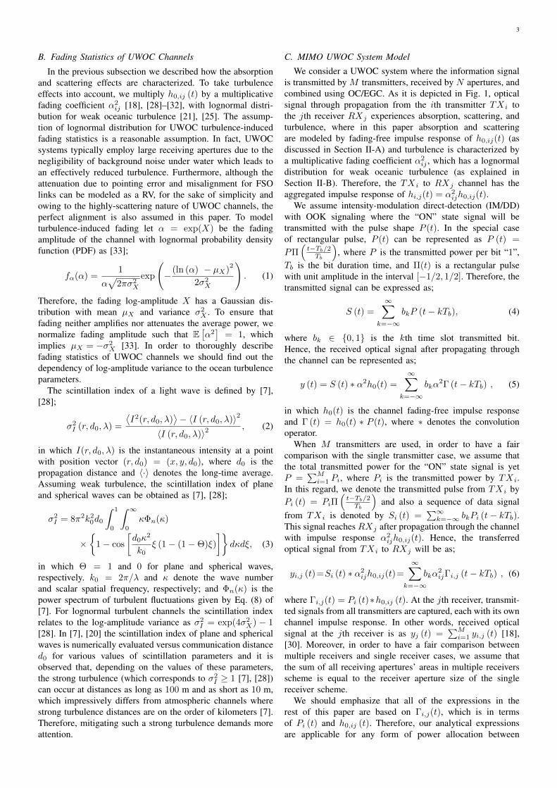
Fig. 1. Block diagram of the MIMO UWOC system with OOK modulation.
studies on the fading statistics of UWOC channels in thepresence of air bubbles have quite recently been carried outin [24].
Despite all of the valuable research have been done onvarious aspects of UWOC, a comprehensive study on theperformance of UWOC systems that takes all degrading effectsof the channel into account is missing in the literature. Whilesome work only considered absorption and scattering effectsand used numerical simulations, without analytical calcula-tions, to estimate the BER of point-to-point UWOC systems[1], some others considered turbulence effects, but neglectedscattering and ISI effects, and used the common conditionalBER expressions in free-space optics (FSO) [21], [25]. Theresearch in this paper is inspired by the need to comprehen-sively evaluate the BER of UWOC systems with respect toall impairing effects of the channel. Moreover, we employmultiple-input multiple-output (MIMO) transmission to inves-tigate how MIMO technique can mitigate turbulence effectsand extend the viable communication range. The technique ofspatial diversity, i.e., exploiting multiple transmitter/receiverapertures (see Fig. 1), not only compensates for fading effects,but can also effectively decrease the possibility of temporaryblockage of the optical beam by obstruction (e.g., fish). An-other advantage of spatial diversity is in reducing the transmitpower density by dividing the total transmitted power by thenumber of transmitters. In other words, depending on thewavelength used there exist some limitations on the maximumallowable safe transmitted power. Hence, by employing spatialdiversity one can increase the total transmitted power by thenumber of transmitters and therefore support longer distances,while maintaining the safe transmit power density [18].
In this paper, we apply maximum-likelihood (ML) detectionto analytically obtain the BER expressions for MIMO UWOCsystems with repetition coding across the transmitters1, wheneither an optimal combiner (OC) or an equal gain combiner(EGC) is used. In order to take the absorption and scatteringeffects into account, we obtain the channel impulse responseusing Monte Carlo (MC) simulations similar to [1], [26].Moreover, to characterize the fading effects, we multiply theabove impulse response by a fading coefficient modeled as alognormal random variable (RV) for weak oceanic turbulence[21], [25]. Closed-form solutions for the exact and upper
1Note that because of the positive nature of incoherent wireless opticalcommunications, a non-destructive addition of different transmitters’ intensitysignals appears at the receiver; therefore, full channel diversity can be achievedby using simple repetition coding, i.e., sending the same on-off keying (OOK)symbol from all of the transmitters for each bit interval.
bound BER calculation are provided using the Gauss-Hermitquadrature formula as well as approximation to the sum oflognormal RVs. We also apply the photon-counting approachto evaluate the BER of various configurations in the presenceof shot noise. In our numerical results we consider bothspatially independent and spatially correlated links.
The rest of the paper is organized as follows. In SectionII, we review some necessary theories in the context ofour proposed MIMO UWOC system and the channel underconsideration in this paper. In Section III, we analyticallyobtain both the exact and upper bound BER expressions,when either OC or EGC is used at the receiver side. Wealso apply Gauss-Hermite quadrature formula to effectivelycalculate multi-dimensional integrals with multi-dimensionalfinite series. In order to evaluate the system BER using photon-counting methods, the same steps as Section III are followed inSection IV. Section V presents the numerical results for varioussystem configurations and parameters considering lognormaldistribution for fading statistics of the UWOC channel. AndSection VI concludes the paper.
II. CHANNEL AND SYSTEM MODEL
In this section, we present the channel model that includesall three impairing effects of the medium, followed by theassumptions and system model that we have introduced inthis paper.
A. Absorption and Scattering of UWOC Channels
Propagation of optical beam in underwater medium inducesinteractions between each photon and seawater particles eitherin the form of absorption or scattering. Absorption is an irre-meable process where photons interact with water moleculesand other particles and lose their energy thermally. On theother hand, in the scattering process each photon’s transmitdirection alters, which also can cause energy loss since fewerphotons will be captured by the receiver aperture. Energyloss due to absorption and scattering can be characterized byabsorption coefficient a(λ) and scattering coefficient b(λ), re-spectively, where λ denotes the wavelength of the propagatinglight wave. Moreover, total effects of absorption and scatteringon the energy loss can be described by extinction coefficientc (λ) = a (λ) + b(λ). These coefficients can vary with sourcewavelength λ and water types [1]. It has been shown in [6],[27] that absorption and scattering have their minimum effectsat the wavelength interval 400 nm < λ < 530 nm. Hence,UWOC systems apply the blue/green region of the visible lightspectrum to actualize data communication.
In [1], [26] the channel impulse response has been simulatedbased on MC method with respect to the absorption and scat-tering effects. We also simulate the channel impulse responsesimilar to [1], [26] relying on MC approach. In this paper,the fading-free impulse response between the ith transmitterand the jth receiver is denoted by h0,ij(t). As it is elaboratedin [1], when the source beam divergence angle and the linkdistance increase the channel introduces more ISI and losson the received optical signal. On the other hand, increasingthe receiver field of view (FOV) and aperture size increasesthe channel delay spread while decreasing its loss. It is worthmentioning that although this behavior may be unobservable inclear ocean links, as the water turbidity increases and multiplescattering dominates it becomes more apparent.
3
B. Fading Statistics of UWOC Channels
In the previous subsection we described how the absorptionand scattering effects are characterized. To take turbulenceeffects into account, we multiply h0,ij (t) by a multiplicativefading coefficient α2
ij [18], [28]–[32], with lognormal distri-bution for weak oceanic turbulence [21], [25]. The assump-tion of lognormal distribution for UWOC turbulence-inducedfading statistics is a reasonable assumption. In fact, UWOCsystems typically employ large receiving apertures due to thenegligibility of background noise under water which leads toan effectively reduced turbulence. Furthermore, although theattenuation due to pointing error and misalignment for FSOlinks can be modeled as a RV, for the sake of simplicity andowing to the highly-scattering nature of UWOC channels, theperfect alignment is also assumed in this paper. To modelturbulence-induced fading let α = exp(X) be the fadingamplitude of the channel with lognormal probability densityfunction (PDF) as [33];
fα(α) =1
α√
2πσ2X
exp
(− (ln (α) − µX)
2
2σ2X
). (1)
Therefore, the fading log-amplitude X has a Gaussian dis-tribution with mean µX and variance σ2
X . To ensure thatfading neither amplifies nor attenuates the average power, wenormalize fading amplitude such that E
[α2]
= 1, whichimplies µX = −σ2
X [33]. In order to thoroughly describefading statistics of UWOC channels we should find out thedependency of log-amplitude variance to the ocean turbulenceparameters.
The scintillation index of a light wave is defined by [7],[28];
σ2I (r, d0, λ) =
⟨I2(r, d0, λ)
⟩− 〈I (r, d0, λ)〉2
〈I (r, d0, λ)〉2, (2)
in which I(r, d0, λ) is the instantaneous intensity at a pointwith position vector (r, d0) = (x, y, d0), where d0 is thepropagation distance and 〈·〉 denotes the long-time average.Assuming weak turbulence, the scintillation index of planeand spherical waves can be obtained as [7], [28];
σ2I = 8π2k20d0
∫ 1
0
∫ ∞0
κΦn(κ)
×
1− cos
[d0κ
2
k0ξ (1− (1−Θ)ξ)
]dκdξ, (3)
in which Θ = 1 and 0 for plane and spherical waves,respectively. k0 = 2π/λ and κ denote the wave numberand scalar spatial frequency, respectively; and Φn(κ) is thepower spectrum of turbulent fluctuations given by Eq. (8) of[7]. For lognormal turbulent channels the scintillation indexrelates to the log-amplitude variance as σ2
I = exp(4σ2X) − 1
[28]. In [7], [20] the scintillation index of plane and sphericalwaves is numerically evaluated versus communication distanced0 for various values of scintillation parameters and it isobserved that, depending on the values of these parameters,the strong turbulence (which corresponds to σ2
I ≥ 1 [7], [28])can occur at distances as long as 100 m and as short as 10 m,which impressively differs from atmospheric channels wherestrong turbulence distances are on the order of kilometers [7].Therefore, mitigating such a strong turbulence demands moreattention.
C. MIMO UWOC System Model
We consider a UWOC system where the information signalis transmitted by M transmitters, received by N apertures, andcombined using OC/EGC. As it is depicted in Fig. 1, opticalsignal through propagation from the ith transmitter TXi tothe jth receiver RXj experiences absorption, scattering, andturbulence, where in this paper absorption and scatteringare modeled by fading-free impulse response of h0,ij(t) (asdiscussed in Section II-A) and turbulence is characterized bya multiplicative fading coefficient α2
ij , which has a lognormaldistribution for weak oceanic turbulence (as explained inSection II-B). Therefore, the TXi to RXj channel has theaggregated impulse response of hi,j(t) = α2
ijh0,ij(t).We assume intensity-modulation direct-detection (IM/DD)
with OOK signaling where the “ON” state signal will betransmitted with the pulse shape P (t). In the special caseof rectangular pulse, P (t) can be represented as P (t) =
PΠ(t−Tb/2Tb
), where P is the transmitted power per bit “1”,
Tb is the bit duration time, and Π(t) is a rectangular pulsewith unit amplitude in the interval [−1/2, 1/2]. Therefore, thetransmitted signal can be expressed as;
S (t) =
∞∑k=−∞
bkP (t− kTb), (4)
where bk ∈ 0, 1 is the kth time slot transmitted bit.Hence, the received optical signal after propagating throughthe channel can be represented as;
y (t) = S (t) ∗ α2h0(t) =
∞∑k=−∞
bkα2Γ (t− kTb) , (5)
in which h0(t) is the channel fading-free impulse responseand Γ (t) = h0(t) ∗ P (t), where ∗ denotes the convolutionoperator.
When M transmitters are used, in order to have a faircomparison with the single transmitter case, we assume thatthe total transmitted power for the “ON” state signal is yetP =
∑Mi=1 Pi, where Pi is the transmitted power by TXi.
In this regard, we denote the transmitted pulse from TXi byPi (t) = PiΠ
(t−Tb/2Tb
)and also a sequence of data signal
from TXi is denoted by Si (t) =∑∞k=−∞ bkPi (t− kTb).
This signal reaches RXj after propagation through the channelwith impulse response α2
ijh0,ij(t). Hence, the transferredoptical signal from TXi to RXj will be as;
yi,j (t)=Si (t) ∗ α2ijh0,ij(t)=
∞∑k=−∞
bkα2ijΓi,j (t− kTb) , (6)
where Γi,j(t) = Pi (t)∗h0,ij (t). At the jth receiver, transmit-ted signals from all transmitters are captured, each with its ownchannel impulse response. In other words, received opticalsignal at the jth receiver is as yj (t) =
∑Mi=1 yi,j (t) [18],
[30]. Moreover, in order to have a fair comparison betweenmultiple receivers and single receiver cases, we assume thatthe sum of all receiving apertures’ areas in multiple receiversscheme is equal to the receiver aperture size of the singlereceiver scheme.
We should emphasize that all of the expressions in therest of this paper are based on Γi,j(t), which is in termsof Pi (t) and h0,ij (t). Therefore, our analytical expressionsare applicable for any form of power allocation between

4
different transmit apertures, any pulse shape of transmittedsignal Pi (t), and any channel model. However, our numericalresults are based on equal power allocation for transmitters,i.e., Pi = P/M, i = 1, . . . ,M , rectangular pulse for OOKsignaling, MC-based simulated channel impulse response, andlognormal distribution for fading statistics. Additionally, allof the derivations throughout the paper are for a generalcase from the transmitters and receivers structures point ofview, i.e., all of the transmitters and receivers are located inarbitrary places. This generality is covered by considering aspecific impulse response for any transmitter-to-receiver pairas hi,j(t) = α2
ijh0,ij(t). However, in our numerical resultswe assume that all of the transmitters and also all of thereceivers are located with an equal separation distance in aline perpendicular to the transmission direction.
III. BER ANALYSIS
In this section, we analytically derive the exact and an upperbound BER expressions for both single-input single-output(SISO) and MIMO schemes, when either OC or EGC is used.Various noise components, i.e., background light, dark current,thermal noise, and signal-dependent shot noise all affect thesystem performance. Since these components are additive andindependent of each other, in this section we model them asan equivalent noise component with Gaussian distribution [34].Also as it is shown in [35], the signal-dependent shot noise hasa negligible effect with respect to the other noise components.Hence, it is amongst the other assumptions of this section toconsider the noise variance independent to the incoming signalpower. Moreover, we assume symbol-by-symbol processing atthe receiver side, which is suboptimal in the presence of ISI[36]. In other words, the receiver integrates its output currentover each Tb seconds and then compares the result with anappropriate threshold to detect the received data bit. In thisdetection process, the availability of channel state information(CSI) is also assumed for threshold calculation.
A. SISO UWOC Link
Based on Eq. (5), the photodetector’s 0th time slot integratedcurrent in SISO scheme can be expressed as;
r(b0)SISO = b0α
2γ(s) + α2−1∑
k=−L
bkγ(I,k) + vTb
, (7)
where γ(s) = R∫ Tb
0Γ(t)dt, γ(I,k) = R
∫ Tb
0Γ(t − kTb)dt =
R∫ −(k−1)Tb
−kTbΓ(t)dt, and R = ηq/hf is the photodetector’s
responsivity. Moreover, η, q, h, f , and L are the photodetec-tor’s quantum efficiency, electron’s charge, Planck’s constant,optical source frequency, and channel memory, respectively.Physically, γ(I,k 6=0) refers to the ISI effect and γ(I,k=0)
interprets the desired signal contribution, i.e., γ(I,k=0) = γ(s).Furthermore, vTb
is the receiver integrated noise componentwhich has a Gaussian distribution with mean zero and varianceσ2Tb
[34]. Note that based on the numerical results presentedin [17], the channel correlation time is on the order of 10−5 to10−2 seconds which implies that thousands up to millions ofconsecutive bits have the same fading coefficient. Therefore,we have adopted the same fading coefficient for all of theconsecutive bits in Eq. (7).
Assuming the availability of CSI, the receiver compares itsintegrated current over each Tb seconds with an appropriate
threshold, i.e., with T = α2γ(s)/2. Therefore, the conditionalprobabilities of error when bits “1” and “0” are transmittedcan respectively be obtained as;
P SISObe|1,α,bk = Pr(r
(b0)SISO ≤ T |b0 = 1)
= Q
α2[γ(s)/2 +
∑−1k=−L bkγ
(I,k)]
σTb
, (8)
P SISObe|0,α,bk = Pr(r
(b0)SISO ≥ T |b0 = 0)
= Q
α2[γ(s)/2−
∑−1k=−L bkγ
(I,k)]
σTb
, (9)
where Q (x) = (1/√
2π)∫∞x
exp(−y2/2)dy is the Gaussian-Q function. Then the final BER can be obtained by averagingthe conditional BER P SISO
be|α,bk = 12P
SISObe|0,α,bk + 1
2PSISObe|1,α,bk over
fading coefficient α and all 2L possible data sequences for bksas;
P SISObe =
1
2L
∑bk
∫ ∞0
P SISObe|α,bkfα(α)dα. (10)
The forms of Eqs. (8) and (9) suggest an upper bound onthe system BER, from the ISI point of view. In other words,bk 6=0 = 0 maximizes (8), while (9) has its maximum value forbk 6=0 = 1. Indeed, when data bit “0” is sent, the worst effectof ISI occurs when all of the surrounding bits are “1” (i.e.,when bk 6=0 = 1), and vice versa [36]. Regarding these specialsequences, the upper bound on the BER of SISO UWOCsystem can be evaluated as;
P SISObe,UB =
1
2
∫ ∞0
[Q
(α2γ(s)
2σTb
)+
Q
α2[γ(s)/2−
∑−1k=−L γ
(I,k)]
σTb
]fα(α)dα. (11)
The averaging over fading coefficient in (10) and (11)involves integrals of the form
∫∞0Q(Cα2)fα(α)dα, where
C is a constant, e.g., C = γ(s)/2σTbin the first integral of
(11). Such integrals can effectively be calculated using Gauss-Hermite quadrature formula [37, Eq. (25.4.46)] as;∫ ∞
0
Q(Cα2)fα(α)dα
=
∫ ∞−∞
Q(Ce2x)1√
2πσ2X
exp
(− (x− µX)2
2σ2X
)dx
≈ 1√π
U∑q=1
wqQ
(C exp
(2xq
√2σ2
X + 2µX
)), (12)
in which U is the order of approximation, wq, q = 1, 2, ..., U ,are weights of the U th-order approximation and xq is the qthzero of the U th-order Hermite polynomial, HU (x) [18], [37].
B. MIMO UWOC Link with OC
Relying on (6), the integrated current of the jth receiver canbe expressed as;
r(b0)j = b0
M∑i=1
α2ijγ
(s)i,j +
M∑i=1
α2ij
−1∑k=−Lij
bkγ(I,k)i,j + v
(j)Tb, (13)

5
where γ(s)i,j = R
∫ Tb
0Γi,j(t)dt, γ
(I,k)i,j = R
∫ Tb
0Γi,j(t −
kTb)dt = R∫ −(k−1)Tb
−kTbΓi,j(t)dt, Li,j is the memory of the
channel between the ith transmitter and jth receiver, and v(j)Tb
is the jth receiver integrated noise which has a Gaussiandistribution with mean zero and variance σ2
Tb. It is worth
mentioning that while EGC simply adds the output of eachreceiving branch (with equal gain) to construct the combinedoutput, the OC applies maximum a posteriori (MAP) detectionrule (which in the case of symbols with equal probabilitysimplifies to ML rule) to obtain the optimal combining policy.
Using the derived decision rule in Appendix A, we findthe “ON” and “OFF” states conditional error probabilities asEqs. (14) and (15), respectively, shown at the top of the nextpage. Assuming the maximum channel memory as Lmax =maxL11, L12, ..., LMN, the average BER of MIMO UWOCsystem can be obtained by averaging over fading coefficientsvector ~α (through an (M ×N )-dimensional integral) as wellas averaging over all 2Lmax possible sequences for bks, i.e.,
PMIMObe,OC =
1
2Lmax
∑bk
∫~α
1
2
[PMIMObe,OC|1,~α,bk+
PMIMObe,OC|0,~α,bk
]f~α(~α)d~α, (16)
where f~α(~α) is the joint PDF of fading coefficients in ~α.Furthermore, considering the transmitted data sequences as
bk 6=0 = 1 for b0 = 0 and bk 6=0 = 0 for b0 = 1, the upperbound on the BER of MIMO UWOC system can be obtainedas Eq. (17), shown at the top of the next page. Moreover, asit is shown in Appendix B, (M × N )-dimensional integralsin (16) and (17) can effectively be calculated by (M × N )-dimensional series using Gauss-Hermite quadrature formula.
It is worth mentioning that for transmitter diversity (N = 1)the conditional BER expressions in (14) and (15) simplify to;
PMISObe|b0,~α,bk =
Q
(M∑i=1
α2i1
[γ(s)i,1 +(−1)b0+1
−1∑k=−Li1
2bkγ(I,k)i,1
]/2σTb
), (18)
which can be reformulated as PMISObe|b0,~α,bk =
Q(∑M
i=1 α2i1G
(b0)i,1
), where G
(b0)i,1 = [γ
(s)i,1 +
(−1)b0+1∑−1k=−Li1
2bkγ(I,k)i,1 ]/2σTb
. The weighted sumof RVs in (18) can be approximated by an equivalentRV, using moment matching method [38]. Therefore,we can approximate the conditional BER of (18) asPMISObe|b0,~α,bk ≈ Q
(G
(b0)M
), where G
(b0)M is the equivalent RV
resulted from the approximation to the weighted sum of RVs,i.e., G(b0)
M ≈∑Mi=1 α
2i1G
(b0)i,1 . In the special case of lognormal
fading, the equivalent lognormal RV, G(b0)M = exp(2z(b0)),
has the log-amplitude mean and variance of;
µz(b0) =1
2ln
( M∑i=1
G(b0)i,1
)− σ2
z(b0) , (19)
σ2z(b0) =
1
4ln
1 +
∑Mi=1
(G
(b0)i,1
)2 (e4σ
2Xi1 − 1
)(∑M
i=1G(b0)i,1
)2 , (20)
respectively [33]. Hence, in the case of transmitter diversitythe average BER can approximately be evaluated with a one-dimensional integral which can also be calculated using Gauss-Hermite quadrature formula as a one-dimensional series.
C. MIMO UWOC Link with EGC
When EGC is used, the integrated current of the receiveroutput, based on Eq. (6), can be expressed as;
r(b0)MIMO =b0
N∑j=1
M∑i=1
α2ijγ
(s)i,j +
N∑j=1
M∑i=1
α2ij
−1∑k=−Lij
bkγ(I,k)i,j + v
(N)Tb
,
(21)
where v(N)Tb
is the integrated combined noise component whichhas a Gaussian distribution with mean zero and variance Nσ2
Tb
[35].Based on (21) and the availability of CSI, the receiver
selects the threshold value as T =∑Nj=1
∑Mi=1 α
2ijγ
(s)i,j /2.
Pursuing similar steps as Section III-B results to (22) forthe conditional BER. As expected, (22) simplifies to (18) forMISO scheme. Finally, the average BER can be evaluatedsimilar to (16). Also the upper bound on the BER of MIMOUWOC system with EGC can be expressed as Eq. (23), shownat the top of the next page.
It is worth noting that the numerator of (22) can beapproximated as ζ(b0) ≈
∑Nj=1
∑Mi=1D
(b0)i,j α
2ij , where
the weight coefficients are defined as D(b0)i,j = γ
(s)i,j +
(−1)b0+1∑−1k=−Lij
2bkγ(I,k)i,j . Similar to (19) and (20), statis-
tics of the equivalent lognormal RV ζ(b0), which is resultedfrom weighted sum of M × N RVs, can be obtained andthen averaging over fading coefficients reduces to the one-dimensional integral of;
PMIMObe,EGC|b0,bk ≈
∫ ∞0
Q
(ζ(b0)
2√NσTb
)fζ(b0)(ζ(b0))dζ(b0),
(24)
which can also effectively be calculated using Eq. (12).
IV. BER EVALUATION USING PHOTON-COUNTINGMETHODS
In this section, we derive the required expressions for thesystem BER using photon-counting approach. Moreover, inthis section signal-dependent shot noise, dark current, andbackground light all are considered with Poisson distribution,while thermal noise is assumed to be Gaussian distributed[36]. To evaluate the BER, we can apply either saddle-pointapproximation or Gaussian approximation which is simplerbut negligibly less accurate than saddle-point approximation.Based on saddle-point approximation the system BER can beobtained as Pbe = 1
2 [q+ (β) + q−(β)], in which q+(β) andq−(β) are probabilities of error when bits “0” and “1” aresent, respectively, i.e.,
q+ (β) = Pr (u > β|zero) ≈ exp [Φ0(s0)]√2πΦ
′′0 (s0)
,
q− (β) = Pr (u ≤ β|one) ≈ exp [Φ1(s1)]√2πΦ
′′1 (s1)
,
Φb0 (s) = ln [Ψu(b0) (s)]− sβ − ln |s| , b0 = 0, 1, (25)
where u is the photoelectrons count at the receiver output andΨu(b0) (s) is the receiver output moment generating function(MGF) when bit “b0” is sent. Also s0 is the positive and realroot of Φ
′
0(s), i.e., Φ′
0(s0) = 0 and s1 is the negative and realroot of Φ
′
1(s), i.e., Φ′
1(s1) = 0; and β is the receiver optimumthreshold and will be chosen such that it minimizes the error

6
PMIMObe,OC|1,~α,bk = Pr
N∑j=1
2rj
M∑i=1
α2ijγ
(s)i,j ≤
N∑j=1
(M∑i=1
α2ijγ
(s)i,j
)2 ∣∣∣rj =
M∑i=1
α2ijγ
(s)i,j +
M∑i=1
α2ij
−1∑k=−Lij
bkγ(I,k)i,j + v
(j)Tb, ~α, bk
= Pr
N∑j=1
[2v
(j)Tb
M∑i=1
α2ijγ
(s)i,j
]≤ −
N∑j=1
M∑i′=1
α2i′jγ
(s)i′,j
M∑i=1
α2ij
γ(s)i,j + 2
−1∑k=−Lij
bkγ(I,k)i,j
= Q
∑Nj=1
∑Mi′=1 α
2i′jγ
(s)i′,j
∑Mi=1 α
2ij
(γ(s)i,j + 2
∑−1k=−Lij
bkγ(I,k)i,j
)2σTb
√∑Nj=1
(∑Mi=1 α
2ijγ
(s)i,j
)2 . (14)
PMIMObe,OC|0,~α,bk = Q
∑Nj=1
∑Mi′=1 α
2i′jγ
(s)i′,j
∑Mi=1 α
2ij
(γ(s)i,j − 2
∑−1k=−Lij
bkγ(I,k)i,j
)2σTb
√∑Nj=1
(∑Mi=1 α
2ijγ
(s)i,j
)2 . (15)
PMIMObe,OC,UB=
∫~α
1
2
Q√∑N
j=1
(∑Mi=1α
2ijγ
(s)i,j
)22σTb
+Q
∑Nj=1
∑Mi′=1α
2i′jγ
(s)i′,j
∑Mi=1α
2ij
(γ(s)i,j −2
∑−1k=−Lij
γ(I,k)i,j
)2σTb
√∑Nj=1
(∑Mi=1 α
2ijγ
(s)i,j
)2f~α(~α)d~α.
(17)
PMIMObe,EGC|b0,~α,bk = Q
∑Nj=1
∑Mi=1 α
2ijγ
(s)i,j + (−1)b0+1
∑Nj=1
∑Mi=1 α
2ij
∑−1k=−Lij
2bkγ(I,k)i,j
2√NσTb
. (22)
PMIMObe,EGC,UB =
∫~α
1
2
[Q
(∑Nj=1
∑Mi=1 α
2ijγ
(s)i,j
2√NσTb
)+Q
∑Nj=1
∑Mi=1 α
2ij
[γ(s)i,j − 2
∑−1k=−Lij
γ(I,k)i,j
]2√NσTb
]f~α(~α)d~α. (23)
probability, i.e., dPbe/dβ = 0. As an another approach toevaluate the system BER, Gaussian approximation is very fastand computationally efficient, yet not as accurate as saddle-point approximation, but yields an acceptable estimate of thesystem error rate particularly for BER values smaller than 0.1[36]. Indeed, when the receiver output is as u = N + ξ,where N is a Poisson distributed RV with mean m(b0) for thetransmitted bit “b0” and ξ is a Gaussian distributed RV withmean zero and variance σ2, Gaussian approximation whichapproximatesN as a Gaussian distributed RV with equal meanand variance results to the following equation for the systemBER [36];
Pbe = Q
(m(1) −m(0)
√m(1) + σ2 +
√m(0) + σ2
). (26)
In this section, the required expressions for both the exact andthe upper bound BER evaluations using either saddle-point orGaussian approximation are presented, when EGC is used atthe receiver side.
A. SISO Configuration
Based on Eq. (5), the photo-detected signal generated bythe integrate-and-dump circuit of the SISO receiver can beexpressed as;
u(b0)SISO = y
(b0)SISO + vth, (27)
where vth corresponds to the receiver integrated thermalnoise and is a Gaussian distributed RV with mean zero andvariance σ2
th = 2KbTrTb/(RLq2), where Kb, Tr, and RL are
Boltzmann’s constant, the receiver equivalent temperature, andload resistance, respectively [39]. Conditioned on bk−1k=−Land α, y(b0)SISO is a Poisson distributed RV with mean m
(b0)SISO
as;
m(b0)SISO =
ηα2
hf
0∑k=−L
bk
∫ Tb
0
Γ (t− kTb) dt+(nb+nd)Tb, (28)
in which nb and nd are mean count rates of Poisson distributedbackground radiation and dark current noise, respectively.
As it is shown in Appendix C, conditioned on α the receiveroutput MGF can be expressed as;
Ψu(b0)
SISO|α(s) = exp
(s2σ2
th
2+[m
(bd)SISO + b0α
2m(s)]
(es − 1)
)×−1∏
k=−L
[1 + exp
(α2m(I,k) (es−1)
)2
], (29)
in which m(bd)SISO = (nb + nd)Tb, m(s) = η
hf
∫ Tb
0Γ(t)dt, and
m(I,k) = ηhf
∫ Tb
0Γ(t− kTb)dt = η
hf
∫ (−k+1)Tb
−kTbΓ(t)dt. More-
over, assuming the transmitted data sequences as bk 6=0 = 1 forb0 = 0 and bk 6=0 = 0 for b0 = 1, MGF of the receiver output

7
for evaluation of upper bound on the BER of SISO UWOCsystem can be obtained as;
ΨUB
u(b0)
SISO|α(s) = exp
(s2σ2
th
2+
[m
(bd)SISO + b0α
2m(s)
+
−1∑k=−L
b0α2m(I,k)
](es − 1)
), (30)
where b0 = 1− b0. Inserting (29) and (30) in (25) results intothe conditional BER, Pbe|α, and the final BER can then beobtained by averaging over the fading coefficient α.
B. MIMO Configuration with EGC
In this scheme, each of N receiving apertures receivesthe sum of all transmitters signals. At the receiver side,each of these N received signals passes through its receiverphotodetector and different types of noises are added to eachoutput. Therefore, the photo-detected signal at the jth receivergenerated by integrate-and-dump circuit can be expressed asu(b0)j = y
(b0)j +vth,j , where vth,j is a Gaussian distributed RV
with mean zero and variance σ2th,j = σ2
th corresponding to theintegrated thermal noise of the jth receiver and y
(b0)j condi-
tioned on bk−1k=−Lijand αijMi=1 is a Poisson distributed
RV with mean;
m(b0)j =
η
hf
M∑i=1
0∑k=−Lij
α2ijbk
∫ Tb
0
Γi,j (t−kTb)dt+(nd,j+nb,j)Tb,
(31)
where nb,j and nd,j are the mean count rates of Pois-son distributed background radiation and dark current noiseof the jth receiver, respectively. As it is demonstratedin Appendix D, MGF of the receiver output in MIMOscheme conditioned on fading coefficients vector ~α =(α11, α12, ..., αMN ) can be expressed as Eq. (32),2 in whichm
(bd)MIMO = (nb +Nnd)Tb, m
(s)i,j = η
hf
∫ Tb
0Γi,j(t)dt, and
m(I,k)i,j = η
hf
∫ Tb
0Γi,j(t− kTb)dt = η
hf
∫ (−k+1)Tb
−kTbΓi,j(t)dt.
Furthermore, MGF of the receiver output for the evaluation ofthe upper bound on the BER of MIMO UWOC system canbe expressed as Eq. (33), shown at the top of the next page.
We should emphasize that extracting the output MGFs forMISO and single-input multiple-output (SIMO) schemes isstraightforward by respectively substituting N = 1 and M = 1
in (32) and (33). Note that for these cases m(bd)MISO = m
(bd)SISO
and m(bd)SIMO = m
(bd)MIMO. Eventually, using saddle-point ap-
proximation the conditional BER Pbe|~α can be achieved byinserting (32) and (33) in (25). The final BER can then beevaluated by averaging over ~α as Pbe =
∫~αPbe|~αf~α (~α)d~α.
With respect to the above complex expressions, usingsaddle-point approximation for BER evaluation may be dif-ficult and computationally time-consuming, since it needs tosolve some complicated equations for which their complexityincreases as ISI (or equivalently Lmax in (32)) increases. But(26) suggests that using Gaussian approximation is simple and
2Note that each of the receivers introduces a Gaussian distributed thermalnoise with mean zero and variance σ2
th,j = σ2th and a Poisson distributed
dark current with mean count of nd,jTb = ndTb. But mean of the Poissondistributed background noise is proportional to the receiver aperture size andwe assumed that the sum of all receiving apertures is identical to the aperturesize of MISO scheme, which implies that
∑Nj=1 nb,j = nb.
computationally fast. It can easily be shown that conditionedon bk the receiver output signal is the sum of a Gaussianand a Poisson RVs; therefore, Gaussian approximation can beapplied to evaluate the average BER conditioned on ~α and bk,i.e., Pbe|~α,bk . The Gaussian distributed RV has mean zero andvariance Nσ2
th. And the Poisson distributed RV has mean of;
m(b0)MIMO =m
(bd)MIMO+
N∑j=1
M∑i=1
b0α2ijm
(s)i,j +
−1∑k=−Lij
bkα2ijm
(I,k)i,j
.(34)
Moreover, mean of the Poisson distributed RV for the evalu-ation of the upper bound on the BER of UWOC system caneasily be obtained by assuming the transmitted data sequencesas bk 6=0 = 1 for b0 = 0 and bk 6=0 = 0 for b0 = 1.
Using (26) and (34) the conditional BER, Pbe|~α,bk , caneasily be evaluated based on Gaussian approximation. More-over, to obtain Pbe|~α,bk based on saddle-point approxima-tion, the simplified form of saddle-point approximation [36,Eqs. (5.73)-(5.79)] can be applied to (34). Subsequently,Pbe|bk can be obtained through an (M × N )-dimensionalintegration as Pbe|bk =
∫~αPbe|~α,bkf~α (~α)d~α which yet
demands excessive computational time, especially for largenumber of links. Nevertheless, we can reformulate (34) asm
(b0)MIMO = m
(bd)MIMO +
∑Nj=1
∑Mi=1
[τ(b0)i,j α2
ij
], where τ (b0)i,j =
b0m(s)i,j +
∑−1k=−Lij
bkm(I,k)i,j . Hence, we can approximate
(34) as m(b0)MIMO ≈ m
(b0)MIMO = m
(bd)MIMO + ϑ(b0), where
m(b0)MIMO is the approximated version of (34) and ϑ(b0) ≈∑Nj=1
∑Mi=1 τ
(b0)i,j α2
ij , i.e., the weighted sum of M ×N RVs.In the special case of weak oceanic turbulence the equivalentlognormal RV, ϑ(b0) = exp(2z(b0)), has the following log-amplitude mean and variance, respectively [33];
µz(b0) =1
2ln
( N∑j=1
M∑i=1
τ(b0)i,j
)− σ2
z(b0) , (35)
σ2z(b0) =
1
4ln
1 +
∑Nj=1
∑Mi=1
(τ(b0)i,j
)2 (e4σ2
Xij − 1)
(∑Nj=1
∑Mi=1 τ
(b0)i,j
)2 .
(36)
By means of the above approximation, Pbe|bk canbe evaluated through two-dimensional integral ofPbe|bk ≈
∫∞0
∫∞0Pbe|bk,ϑ(0),ϑ(1)f(ϑ(0), ϑ(1))dϑ(0)dϑ(1),
where Pbe|bk,ϑ(0),ϑ(1) is the system BER conditioned on bk,ϑ(0) and ϑ(1), and (when Gaussian approximation is used)can be obtained as;
Pbe|bk,ϑ(0),ϑ(1)≈Q
m(1)MIMO − m
(0)MIMO√
m(1)MIMO+Nσ2
th+
√m
(0)MIMO+Nσ2
th
.
(37)
Note that in the MISO scheme all of the transmitters arepointed to a single receiver; therefore, all of the links havethe same fading-free impulse response and channel mem-ory as h0,MISO(t) and LMISO, respectively. Consequently,when all transmitters have identical transmitted power ofP/M , all links have equal m(s)
i,1 and m(I,k)i,1 as m(s)
MISO andm
(I,k)MISO, respectively. Hence, we can rewrite (34) as m(b0)
MISO =
m(bd)MISO+
(b0m
(s)MISO +
∑−1k=−LMISO
bkm(I,k)MISO
)ϕ(M), where

8
ΨEGC
u(b0)
MIMO|~α(s)=exp
Nσ2th
2s2+
m(bd)MIMO+
N∑j=1
M∑i=1
b0α2ijm
(s)i,j
(es−1)
× N∏j=1
−1∏k=−Lmax
1
2
[1+
M∏i=1
exp(α2ijm
(I,k)i,j (es−1)
)].
(32)
ΨEGC,UB
u(b0)
MIMO|~α(s) = exp
(Nσ2
th
2s2 +
m(bd)MIMO +
N∑j=1
M∑i=1
α2ij
b0m(s)i,j + b0
−1∑k=−Lij
m(I,k)i,j
(es − 1)
). (33)
TABLE ISOME OF THE IMPORTANT PARAMETERS USED FOR NOISE
CHARACTERIZATION AND MC-BASED CHANNEL SIMULATION.
Coefficient Value
Quantum efficiency, η 0.8Optical filter bandwidth, 4λ 10 nmOptical filter transmissivity, TF 0.8Equivalent temperature, Te 290 KLoad resistance, RL 100 ΩDark current, Idc 1.226× 10⁻⁹ AReceiver half angle FOV, θFOV 400
MISO schemes aperture diameter, D(MISO)0 20 cm
Source wavelength, λ 532 nmWater refractive index, n 1.331Source full beam divergence angle, θdiv 0.020
Photon weight threshold at the receiver, wth 10−6
Separation distance between the transmitters andbetween the receiving apertures, l0
25 cm
ϕ(M) =∑Mi=1 α
2i1, i.e., the sum of M lognormal
RVs. As a result, Pbe|bk for MISO scheme can beevaluated through one-dimensional integral of Pbe|bk ≈∫∞0Pbe|bk,ϕ(M)f(ϕ(M))dϕ(M). Then, if the channel memory
is Lmax bits, Pbe can be obtained by averaging as Pbe =1
2Lmax
∑bkPbe|bk . Note that as ISI increases, this averaging
demands more computational time and evaluation of the upperbound BER becomes more advantageous.
From (34), one can observe the destructive effect of ISI onthe BER. In other words, experiencing more time spreadingin h0,ij(t) or equivalently Γi,j(t) increases
∑k 6=0m
(I,k)i,j and
decreases m(s)i,j . Thereby, it causes an increase in m(0) and a
decrease in m(1) which results into larger BERs. Constructiveeffect of spatial diversity is appeared as combining the fadingcoefficients of different links which can be approximated asa single lognormal RV with roughly a scaled log-amplitudevariance by the number of links [18].
V. NUMERICAL RESULTS
In this section, we present the numerical results for theBER performance of UWOC systems in various scenarios.We consider lognormal distribution for the channel fadingstatistics, equal power as P/M for all transmitters, the samefading statistics (log-amplitude variance) for all links and thesame aperture area of A/N for all of the receivers, whereA is the total aperture area. In simulating the turbulence-free impulse response by MC method, we consider coastalwater and also turbid harbor water links with absorption andscattering coefficients of (a, b) = (0.179, 0.219) m−1 and(0.366, 1.824) m−1, respectively [6]. Other important parame-ters for MC simulations are listed in Table I. In addition, someof the important parameters for characterization of noises areaddressed in this table and the other parameters are exactly
the same as those mentioned in [8], [40]. Based on theseparameters, noise characteristics are as nb ≈ 1.8094× 10⁸
s−1 in 30 meters deep coastal water, nd ≈ 76.625× 10⁸ s−1,and σ2
th/Tb = 3.12× 10¹⁵ s−1. Hence, background radiationhas a negligible effect on the system performance.
Moreover, in this section we obtain the BER values usingnumerical simulations to verify the accuracy of our derivedexpressions. To do so, we generate 107 Bernoulli RVs withPDF of Pr(b0) = 1
2δ(b0) + 12δ(b0 − 1), where δ(.) is Dirac
delta function. Subsequently, 107 pulses of shape b0Pi(t) willbe transmitted to the channel. Each of these 107 pulses willbe convolved with the channel fading-free impulse responseand multiplied by a lognormal RV to construct b0α2
ijPi(t) ∗h0,ij(t) = b0α
2ijΓi,j(t). Additionally, a contribution of chan-
nel ISI reaches the receiver as described in Eqs. (7) and (13).At the receiver side, the integrated current will be added bya Gaussian distributed noise and the result will be comparedwith an appropriate threshold (as comprehensively studied inSection III) to detect the received signal. Finally, comparingthe transmitted data sequence with the detected one determinesthe BER value in a specified amount of the transmitted power.
In order to see how water turbidity affects the channel lossand temporal dispersion, and also to investigate the channelspatial beam spread, we use MC method to simulate thechannel fading-free impulse responses for a 1 × 2 SIMOtransmission in a 25 m coastal water link and also an 8 mturbid harbor water link. The transmitter is pointed to thefirst receiver and the link between the transmitter and thefirst receiver has the impulse response of h0,11(t). The secondreceiver is located in 25 cm center-to-center distance fromthe first aperture and receives those photons that are reachedwith much more scattering; with impulse response of h0,12(t).Each receiving aperture has a diameter of 20/
√2 cm. Fig. 2
illustrates the simulation results. Comparing Figs. 2(a) and2(c) shows that while the direct link in a 25 m coastal waterhas a negligible scattering, an 8 m turbid harbor water linkremarkably scatters propagating photons and induces muchmore delay spread on h0,11(t). In other words, as the waterturbidity increases both the channel loss and delay spreadconsiderably raise. As a result, an 8 m turbid harbor water linkhas a poor channel condition even than a 25 m coastal waterlink. Moreover, comparing Figs. 2(a) and 2(b) demonstratesthat the second receiver mainly receives those photons thathave experienced more scattering than the received photonsby the first aperture. Accordingly, the channel delay spread inh0,12(t) is by far more than h0,11(t).
Fig. 3 depicts the exact BER of a 25 m coastal waterlink with transmitter diversity and data transmission rate ofRb = 1 Gbps. This figure also indicates an excellent matchbetween the results of analytical expressions and numerical

9
0 1 2 3 4 5
x 10−11
0
2
4
6
x 10−5
time [s]
Nor
mal
ized
Inte
nsity h
11(t), 25 m coastal water link
(a)
−1 0 1 2 3 4 5
x 10−10
0
0.5
1
1.5x 10
−6
time [s]
Nor
mal
ized
Inte
nsity h
12(t), 25 m coastal water link
(b)
0 2 4 6 8
x 10−9
0
1
2
3
x 10−6
time [s]
Nor
mal
ized
Inte
nsity
h11
(t), 8 m turbid harbor water link
(c)
1
Fig. 2. Fading-free impulse responses for a 1× 2 SIMO UWOC system in different water types. (a) h0,11(t) of a 25 m coastal water link; (b) h0,12(t) ofa 25 m coastal water link; (c) h0,11(t) of an 8 m turbid harbor water link.
5 10 15 20 25 30 35 4010−15
10−10
10−5
100
Average transmitted power per bit [dBm]
Ave
rage
BE
R
SISO,Analytical2×1 MISO,Analytical3×1 MISO,AnalyticalSISO, Num. Sim.2×1 MISO, Num. Sim.3×1 MISO, Num. Sim.
σX
=0.1
σX
=0.4
Fig. 3. Exact BER of a 25 m coastal water link with SISO, 2 × 1 MISOand 3 × 1 MISO configurations, obtained using both analytical expressionsand numerical simulations. Rb = 1 Gbps, σX = 0.1 and 0.4.
simulations. Here, we assume that the fading of each link isindependent from the others. As it is obvious, increasing thenumber of independent links provides significant performanceimprovement in the case of σX = 0.4, e.g., one can achieveapproximately 6 dB and 9 dB performance improvement at theBER of 10−12, using two and three transmitters, respectively.But this benefit relatively vanishes in very weak fading condi-tions, e.g., σX = 0.1. This is reasonable, since in very weakturbulence conditions fading has a minuscule effect on theperformance but scattering and absorption have yet substantialeffects. Hence, in such scenarios multiple transmitters scheme,which combats with impairing effects of fading, does notprovide a notable performance improvement.
In Fig. 4, we assume the same parameters as in Fig. 3and use our derived analytical expressions to evaluate theexact BER of 1 × 2 SIMO, 1 × 3 SIMO and 2 × 2 MIMOconfigurations with optimal/equal gain combiner. Comparisonbetween the results shows that the performance of EGC isvery close to the performance of OC receiver. Therefore, dueto its lower complexity, receiver with EGC is more practicallyinteresting. Furthermore, the good match between the analyti-cal results and numerical simulations confirms the accuracyof our derived analytical expressions for the system BER.Comparing the results of BER for SISO and SIMO schemesdemonstrates that a 1 × N ′ SIMO scheme provides betterperformance than a 1×N SIMO configuration (N ′ > N ≥ 1)only at high signal-to-noise ratios (SNRs) or equivalently low
5 10 15 20 25 30 35 4010−15
10−10
10−5
100
Average transmitted power per bit [dBm]
Ave
rage
BE
R
1×2 SIMO, EGC, Analytical1×3 SIMO, EGC, Analytical2×2 MIMO, EGC, Analytical1×2 SIMO, OC, Analytical1×3 SIMO, OC, Analytical2×2 MIMO, OC, AnalyticalNumerical Simulation Results
σX
=0.1
σX
=0.4
Fig. 4. Exact BER of a 25 m coastal water link with 1×2 SIMO, 1×3 SIMOand 2 × 2 MIMO configurations and optimal/equal gain combiner, obtainedusing both analytical expressions and numerical simulations. Rb = 1 Gbps,σX = 0.1 and 0.4.
BERs, where fading has more impairing effect than absorptionand ISI. This is reasonable, since each receiver in a 1 × N ′SIMO scheme has N ′/N times less aperture area than a 1×NSIMO configuration and also an N ′-receiver scheme imposesN ′/N times more dark current and thermal noise. In lowSNRs, absorption and scattering as well as noise have moredominant effects on the BER than fading; therefore, in lowSNRs the 1 × N SIMO scheme yields better performancethan the 1×N ′ SIMO structure. However, when the channelsuffers from relatively notable turbulence, the 1 × N ′ SIMOstructure which has more links can better mitigate fading andcan compensate for the loss due to the smaller aperture sizeand excess noise and therefore can yield better performanceat higher SNRs. Needless to say that a 2× 2 MIMO structurehas the same aperture size as a 1 × 2 SIMO structure andsince benefits from more independent links can yield betterperformance, than a 1×N ′ SIMO, in all ranges of SNR. Onecan expect that in a very weak turbulence scenario, such asσX = 0.1, dividing the receiver aperture to extend the numberof independent links can degrade the performance.
In Fig. 5 we applied our derived analytical expressions toevaluate the exact and upper bound BERs of a 25 m coastalwater link with Rb = 1 Gbps and σX = 0.4, using (M ×N )-dimensional integrals. As it can be seen, the upper boundBER curves have good tightness with the exact BER curves.Therefore, the upper bound BER evaluation can be more

10
10 15 20 25 30 35 4010−15
10−10
10−5
100
Average transmitted power per bit [dBm]
Ave
rage
BE
R
Exact, Analytical, M×N−dimensional integrals
UB, Analytical, M×N−dimensional integrals
UB, Analytical, M×N−dimensional series of GHQF
2×2 MIMO, OC
3×1 MISO
1×3 SIMO, EGC
SISO
1×3 SIMO, OC
2×2 MIMO, EGC
Fig. 5. Comparison between the exact and the upper bound BERs of a 25 mcoastal water link with Rb = 1 Gbps, σX = 0.4, and various configurations.Also the upper bound BERs are calculated with (M×N )-dimensional series,using Gauss-Hermite quadrature formula (GHQF).
10 15 20 25 30 35 4010−15
10−10
10−5
100
Average transmitted power per bit [dBm]
Ave
rage
BE
R
Exact, AnalyticalExact, Gaussian ApproximationExact, Saddle−Point Approximation
2×1 MISO
2×2 MIMO
3×1 MISO
SISO
1×3 SIMO
1×2 SIMO
Fig. 6. Comparing Gaussian and saddle-point approximations in evaluatingthe exact BER of a 25 m coastal water link with Rb = 1 Gbps, σX = 0.4,and various configurations. Also the results of photon-counting methods arecompared with the results of our derived analytical expressions for the systemexact BER.
preferable since the exact BER calculation may need excessivetime for averaging over bks. Furthermore, the upper boundBERs of various configurations are calculated by (M × N )-dimensional series, using Gauss-Hermite quadrature formula(GHQF). The order of approximation U is assumed to bethe same for all of the links, i.e., Uij = 30. The excellentmatch between the results of GHQF and numerical (M ×N )-dimensional integrals demonstrates the usefulness of GHQFin effective calculation of the system BER.
Fig. 6 compares Gaussian and saddle-point approximationsin evaluating the exact BER of a 25 m coastal water link withRb = 1 Gbps, σX = 0.4, and various configurations. It isobserved that Gaussian approximation can provide relativelythe same results as saddle-point approximation. Therefore,due to its simplicity and acceptable accuracy, Gaussian ap-proximation can be considered as a reliable photon-countingmethod for the system BER evaluation. Moreover, the resultsof our derived analytical expressions are compared with thoseof photon-counting methods. The good match between theresults of analytical expressions and photon-counting methodsfurther confirms the validity of our assumption in neglecting
the signal-dependent shot noise in our analytical derivations.
After confirming the accuracy of our derived analyticalexpressions, a comparison between the computation time ofdifferent methods would be interesting. Table II shows thecomputation time and BER values of different methods forvarious system configurations in a 25 m coastal water linkwith σX = 0.4, Rb = 1 Gbps, and average transmitted powerper bit of 20 dBm. The values in this table are obtained through(M × N)-dimensional integration over fading coefficients aswell as averaging over all 2Lmax sequences for bks. In orderto perform the integration, we have taken Nsamp equidistantsamples from the interval αij ∈ [0.0001, 5]. Here, we havechosen Lmax = 3, Nsamp = 30 for MIMO configuration,and Nsamp = 100 for the other schemes. As it can be seen,saddle-point approximation has by order of magnitude largercomputation time, since it involves solving some complexnonlinear equations to obtain the conditional BERs. On theother hand, our derived analytical expressions and Gaussianapproximation have relatively the same calculation time, sinceboth involve Gaussian-Q function which is a fast-calculablebuilt-in function in Matlab. Moreover, all three methods yieldsimilar results for the system average BER, confirming theaccuracy of our derived analytical expressions and the validityof our assumption in Section III, i.e., the negligibility ofsignal-dependent shot noise. A more advantage of our derivedanalytical expressions becomes visible when we apply theapproximation to the sum of RVs. In this case, as it iselaborated in Section III, in the case of transmitter diversity(N = 1) and also receiver diversity with EGC, the (M ×N)-dimensional averaging integration can be evaluated through anequivalent one-dimensional integral using our derived analyti-cal expressions, while Gaussian approximation only in the caseof transmitter diversity leads to a one-dimensional integral, asshown in Section IV. Accordingly, when approximation to thesum of RVs is applied, our derived analytical expressions canmore quickly predict the system performance. Therefore, ouranalytical approach is more advantageous and convenient fromthe computation time and ease of mathematical manipulationpoints of view; and hence is recommended to be employed foranalysis of MIMO UWOC systems.
In Fig. 7, the BER performance of a 25 m coastal water linkwith Rb = 0.5 Gbps and σX = 0.3 is depicted for differentconfigurations. Also the sum of independent lognormal RVsin (34) is approximated with a single lognormal RV andthe BER is evaluated through the approximated one-or two-dimensional integrals. As it can be seen, relatively good matchexists between the results of the approximated one-or two-dimensional integrals and the exact (M ×N)-dimensional in-tegral of Pbe =
∫~αPbe|~αf~α (~α)d~α. However, the discrepancy
increases when receiver diversity is used. Moreover, the BERperformance of a SISO link with σX = 0.1 is compared withthe BER curve of a 9 × 1 MISO link with σX = 0.3, andapproximately the same result is observed; therefore, spatialdiversity manifests its effect as a reduction in the fading log-amplitude variance.
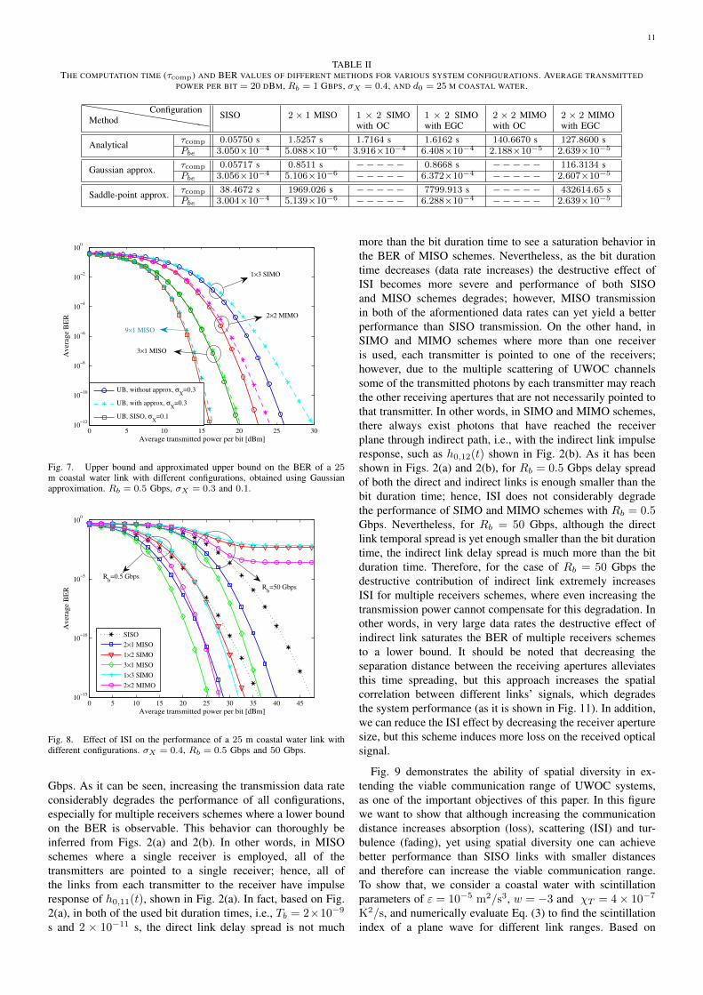
In order to investigate how ISI affects the performance ofdifferent configurations, in Fig. 8 the upper bound on the BERof a 25 m coastal water link with σX = 0.4 and variousconfigurations is illustrated for a typical data rate of Rb = 0.5Gbps and also an extremely large data rate of Rb = 50
11
TABLE IITHE COMPUTATION TIME (τcomp) AND BER VALUES OF DIFFERENT METHODS FOR VARIOUS SYSTEM CONFIGURATIONS. AVERAGE TRANSMITTED
POWER PER BIT = 20 DBM, Rb = 1 GBPS, σX = 0.4, AND d0 = 25 M COASTAL WATER.
hhhhhhhhhhhMethodConfiguration SISO 2× 1 MISO 1 × 2 SIMO
with OC1 × 2 SIMOwith EGC
2 × 2 MIMOwith OC
2 × 2 MIMOwith EGC
Analytical τcomp 0.05750 s 1.5257 s 1.7164 s 1.6162 s 140.6670 s 127.8600 sPbe 3.050×10⁻⁴ 5.088×10⁻⁶ 3.916×10⁻⁴ 6.408×10⁻⁴ 2.188×10⁻⁵ 2.639×10⁻⁵
Gaussian approx. τcomp 0.05717 s 0.8511 s −−−−− 0.8668 s −−−−− 116.3134 sPbe 3.056×10⁻⁴ 5.106×10⁻⁶ −−−−− 6.372×10⁻⁴ −−−−− 2.607×10⁻⁵
Saddle-point approx. τcomp 38.4672 s 1969.026 s −−−−− 7799.913 s −−−−− 432614.65 sPbe 3.004×10⁻⁴ 5.139×10⁻⁶ −−−−− 6.288×10⁻⁴ −−−−− 2.639×10⁻⁵
0 5 10 15 20 25 3010−12
10−10
10−8
10−6
10−4
10−2
100
Ave
rage
BE
R
Average transmitted power per bit [dBm]
UB, without approx, σX
=0.3
UB, with approx, σX
=0.3
UB, SISO, σX
=0.1
3×1 MISO
2×2 MIMO
1×3 SIMO
9×1 MISO
Fig. 7. Upper bound and approximated upper bound on the BER of a 25m coastal water link with different configurations, obtained using Gaussianapproximation. Rb = 0.5 Gbps, σX = 0.3 and 0.1.
0 5 10 15 20 25 30 35 40 4510−15
10−10
10−5
100
Average transmitted power per bit [dBm]
Ave
rage
BE
R
SISO2×1 MISO1×2 SIMO3×1 MISO1×3 SIMO2×2 MIMO
Rb=50 Gbps
Rb=0.5 Gbps
Fig. 8. Effect of ISI on the performance of a 25 m coastal water link withdifferent configurations. σX = 0.4, Rb = 0.5 Gbps and 50 Gbps.
Gbps. As it can be seen, increasing the transmission data rateconsiderably degrades the performance of all configurations,especially for multiple receivers schemes where a lower boundon the BER is observable. This behavior can thoroughly beinferred from Figs. 2(a) and 2(b). In other words, in MISOschemes where a single receiver is employed, all of thetransmitters are pointed to a single receiver; hence, all ofthe links from each transmitter to the receiver have impulseresponse of h0,11(t), shown in Fig. 2(a). In fact, based on Fig.2(a), in both of the used bit duration times, i.e., Tb = 2×10⁻⁹
s and 2 × 10⁻¹¹ s, the direct link delay spread is not much
more than the bit duration time to see a saturation behavior inthe BER of MISO schemes. Nevertheless, as the bit durationtime decreases (data rate increases) the destructive effect ofISI becomes more severe and performance of both SISOand MISO schemes degrades; however, MISO transmissionin both of the aformentioned data rates can yet yield a betterperformance than SISO transmission. On the other hand, inSIMO and MIMO schemes where more than one receiveris used, each transmitter is pointed to one of the receivers;however, due to the multiple scattering of UWOC channelssome of the transmitted photons by each transmitter may reachthe other receiving apertures that are not necessarily pointed tothat transmitter. In other words, in SIMO and MIMO schemes,there always exist photons that have reached the receiverplane through indirect path, i.e., with the indirect link impulseresponse, such as h0,12(t) shown in Fig. 2(b). As it has beenshown in Figs. 2(a) and 2(b), for Rb = 0.5 Gbps delay spreadof both the direct and indirect links is enough smaller than thebit duration time; hence, ISI does not considerably degradethe performance of SIMO and MIMO schemes with Rb = 0.5Gbps. Nevertheless, for Rb = 50 Gbps, although the directlink temporal spread is yet enough smaller than the bit durationtime, the indirect link delay spread is much more than the bitduration time. Therefore, for the case of Rb = 50 Gbps thedestructive contribution of indirect link extremely increasesISI for multiple receivers schemes, where even increasing thetransmission power cannot compensate for this degradation. Inother words, in very large data rates the destructive effect ofindirect link saturates the BER of multiple receivers schemesto a lower bound. It should be noted that decreasing theseparation distance between the receiving apertures alleviatesthis time spreading, but this approach increases the spatialcorrelation between different links’ signals, which degradesthe system performance (as it is shown in Fig. 11). In addition,we can reduce the ISI effect by decreasing the receiver aperturesize, but this scheme induces more loss on the received opticalsignal.
Fig. 9 demonstrates the ability of spatial diversity in ex-tending the viable communication range of UWOC systems,as one of the important objectives of this paper. In this figurewe want to show that although increasing the communicationdistance increases absorption (loss), scattering (ISI) and tur-bulence (fading), yet using spatial diversity one can achievebetter performance than SISO links with smaller distancesand therefore can increase the viable communication range.To show that, we consider a coastal water with scintillationparameters of ε = 10−5 m2/s3, w = −3 and χT = 4× 10⁻⁷
K2/s, and numerically evaluate Eq. (3) to find the scintillationindex of a plane wave for different link ranges. Based on

12
10 15 20 25 30 35 40 45 5010−15
10−10
10−5
100
Average transmitted power per bit [dBm]
Ave
rage
BE
R
25m, 1×1, σ2X
=0.126
30m, 1×1, σ2X
=0.165
30m, 2×1, σ2X
=0.165
30m, 3×1, σ2X
=0.165
30m, 2×2, σ2X
=0.165
30m, 1×1, σ2X
=0.01
Fig. 9. Comparison between the performance of a 30 m coastal water linkwith different configurations and a 25 m SISO link, both operating at Rb = 2Gbps.
our numerical results we find that for d0 = 25 m and30 m the log-amplitude variance σ2
X is 0.126 and 0.165,respectively. As it is obvious in Fig. 9, only 5 m (%20)increase on the communication range remarkably degrades thesystem performance, e.g., approximately 12 dB degradationis observed at the BER of 10−12. But as it can be seen,increasing the number of independent links or equivalentlymitigating fading deteriorations considerably improves thesystem performance. Since spatial diversity manifests itselfas a reduction in fading variance [18], we can conclude thatthere exists a configuration with spatial diversity at link rangeof 30 m which performs similar to a SISO link at that rangebut with less fading variance, e.g., σ2
X = 0.01. Hence, in thisfigure the performance of a 30 m SISO link with σ2
X = 0.01is also depicted for the sake of comparison and obviouslyit can yield better performance than a 25 m SISO link,especially for lower error rates. Therefore, one can achievebetter performance even in longer link ranges by employingspatial diversity technique. We should emphasize that spatialdiversity can provide more performance enhancement ratherthan those are presented in this paper; when the channel suffersfrom strong turbulence [30]. But since this paper is focusedon weak oceanic turbulence, we only considered channels withσ2I < 1 [28].In order to better observe the effects of different factors
on the channel impulse response and hence on the systemperformance, we consider four different channel models andevaluate the BER performance of a SISO UWOC link foreach of the considered channel models. The first model (M1)only considers turbulence effect and ignores absorption andscattering effects, i.e., h1(t) = α2δ(t − d0/v), where v isthe propagation speed of light through water. The secondmodel (M2) only considers absorption and scattering usingBeer’s law [6] and neglects turbulence effect, i.e., h2(t) =e−cd0δ(t − d0/v). The third model (M3) obtains the channelfading-free impulse response using MC numerical simulationsbut ignores turbulence effect, i.e., h3(t) = h0(t). And thefourth model (M4), similar to the rest of the paper, takes allof the three impairing effects into account while considersabsorption and scattering effects based on MC simulations andturbulence effect as a multiplicative fading coefficient, i.e.,
−30 −20 −10 0 10 20 30 40 50 60 7010−12
10−10
10−8
10−6
10−4
10−2
100
Average transmitted power per bit [dBm]
Ave
rage
BE
R
S1, M1S2, M1S1, M2S2, M2S1, M3S2, M3S1, M4S2, M4
Fig. 10. The exact BER of a SISO UWOC link for two separate scenarios(S1: a 25 m coastal water link with Rb = 1 Gbps, and S2: a 10 m turbidharbor water link with Rb = 200 Mbps) and four different models for thechannel impulse response described within the text (M1, M2, M3, and M4).
h4(t) = α2h0(t). We also consider two different scenarios:S1; a 25 m coastal water link with transmission rate Rb = 1Gbps, and S2; a 10 m turbid harbor water link with Rb = 200Mbps. All of the system parameters are the same as those arelisted in Table I, and the log-amplitude variance for both ofthe scenarios is considered to be σ2
X = 0.16. As it is shownin Fig. 10, based on the results of the accurate channel model,i.e., the fourth channel model M4, a 25 m coastal water linkhas approximately 18 dB better performance than a 10 mturbid harbor water link even for 5 times larger transmissionrates. Furthermore, as expected, ignoring the turbulence effectthrough considering the channel impulse response as thethird model M3, underestimates the channel impairments andsignificantly increases the slope of BER curves. On the otherhand, considering the channel impulse response as the secondmodel overestimates the channel attenuation and shifts theBER curves to the right side when compared with the thirdchannel model results. This is because Beer’s law ignoresthose photons which may reach the receiver through multiplescattering. The overestimation of Beer’s law for turbid harborwater link is by far more than that of coastal water linkdue to the higher values of attenuation length defined asτatn = cd0 (for the above two scenarios τatn,S1 = 9.95 andτatn,S2 = 21.9) [1], [14]. In other words, in turbid harborwaters the occurance of multiple scattering is very prevalentand many of the transmitted photons may reach the receiverafter scattering many times, and ignoring multiple scattering insuch links, through use of Beer’s law, results into an extremeoverestimation of the channel loss. Finally, ignoring absorptionand scattering effects and only considering turbulence effectsas a multiplicative fading coefficient, through use of the firstchannel model M1, significantly underestimates the channeldegrading effects and considerably shifts the BER curves to theleft side. This is mainly because in coastal and turbid harborUWOC channels with weak turbulence conditions, absorptionand scattering have much more impairing effects than turbu-lence, and ignoring their effects remarkably underestimates thechannel impairments.
As it has been observed, spatial diversity provides a sig-nificant performance improvement but under the assumptionof independent links which is sometimes practically infeasible

13
15 20 25 3010−10
10−9
10−8
10−7
10−6
10−5
10−4
10−3
10−2
Average transmitted power per bit [dBm]
Ave
rage
BE
R
independent, SISOindependent, 2×1 MISOindependent, 3×1 MISOdependent, 2×1 MISOdependent, 3×1 MISOdependent, 2×2 MIMO
ρ=0.7
ρ=0.25
Fig. 11. Effect of spatial correlation on the performance of a 25 m coastalwater link with σX = 0.4, Rb = 2 Gbps, ρ = 0.25 and 0.7.
[41]. Therefore, in practice received signals by different linksmay have correlation. In Fig. 11, we investigate the effectof spatial correlation on the performance of MIMO UWOCsystems in a similar approach to [18]. Given an M by Mcorrelation matrix at the transmitter side as RT and also an Nby N correlation matrix at the receiver side as RR, the spatialcorrelation matrix of the MIMO channel can be obtainedby the Kronecker product of the spatial correlation matricesof the transmitter and receiver, i.e., RMIMO = RT⊗RR,which is of size M × N by M × N [18]. Then, givenX = [X1, X2, ..., XM×N ] as a vector of M × N Gaussiandistributed RVs with mean zero and variance one, the vectorof new RVs, X′ = [X ′1, X
′2, ..., X
′M×N ], corresponding to
the Gaussian distributed log-amplitude factors with correlationmatrix of RMIMO, can be obtained as;
X′ = σXXC − Σ, (38)
where Σ = [σ2X , ..., σ
2X ] is a vector of M×N elements of σ2
X ,and C is an M×N by M×N upper triangular matrix obtainedfrom the Cholesky decomposition of the correlation matrixRMIMO as RMIMO = C∗C, where C∗ denotes the complexconjugate transpose of C. Finally, the new correlated lognormalRVs, corresponding to the fading coefficients of different links,can be obtained as α′2ij = exp(2X ′ij), and the average BERcan be evaluated from these correlated fading coefficients bynumerical calculation of multi-dimensional integrals. In thesimulations of Fig. 11, we have considered a 25 m coastalwater link with σX = 0.4 and Rb = 2 Gbps, and evaluated theupper bound BER of different configurations in several cases,i.e., independent links and correlated links with correlationvalues of b (l0) = ρ = 0.25 and 0.7. Comparing the resultsshows that the performance loss is much more severe for largercorrelation values, e.g., 2 dB and 6 dB degradation can beobserved in the performance of a 3 × 1 MISO link with theBER of 10−10 and with ρ = 0.25 and 0.7, respectively. Alsoa 3×1 MISO link with ρ = 0.25 yields the same performanceas an independent 2× 1 MISO link, i.e., the diversity order isdecreased by one. Therefore, the performance enhancement ofspatial diversity in highly correlated weak turbulent channelsmay be insignificant.
VI. CONCLUSION
In this paper, we studied the performance of MIMO UWOCsystems with OOK modulation and equal gain or optimalcombiner. Our derivations were based on a general channelmodeling which appropriately takes all of the channel im-pairments into account. In particular, we obtained the channelfading-free impulse response using MC numerical simulationsand included turbulence effects as a multiplicative fading coef-ficient. Closed-form solutions for the system BER expressionsobtained in the case of lognormal underwater fading channels,relying on Gauss-Hermite quadrature formula as well asapproximation to the sum of lognormal random variables. Wealso applied photon-counting method to evaluate the systemBER in the presence of shot noise. The excellent matchbetween the results of analytical expressions and photon-counting method confirmed the validity of our assumptionsin derivation of analytical expressions for the system BER.Furthermore, our numerical results indicated that EGC is morepractically interesting, due to its lower complexity and its closeperformance to optimal combiner. In addition to evaluatingthe exact BER, also the upper bound on the system BERhas been evaluated and excellent tightness between the exactand upper bound BER curves has been observed. Moreover,the good match between the results of numerical simulationsand analytical expressions verified the accuracy of our derivedanalytical expressions for the system BER. Our numericalresults showed that spatial diversity manifests its effect asa reduction in fading variance and hence can significantlyimprove the system performance and increase the viablecommunication range. In particular, a 3×1 MISO transmissionin a 25 m coastal water link with log-amplitude variance of0.16 can introduce 8 dB performance improvement at the BERof 10−9. We also observed that spatial correlation can imposea severe loss on the performance of MIMO UWOC systems.Specifically, correlation value of ρ = 0.25 between the linksof a 3×1 MISO UWOC system with σX = 0.4 decreases theorder of diversity by one. Finally, we should emphasize thatalthough all of the numerical results of this paper are based onlognormal distribution, many of our derivations can be usedfor any other fading statistical distribution.
APPENDIX ADECISION RULE FOR MIMO UWOC SYSTEM WITH OC
In this appendix, we obtain the decision rule for BERevaluation of MIMO UWOC system with OC. Based on theML detection rule and assuming the availability of perfectCSI, the symbol-by-symbol receiver which does not have anyknowledge to bk−1k=−Li,j
, adopts the following metric foroptimum combining [18];
Pr (~r|b0 = 1, ~α)1
≷0
Pr (~r|b0 = 0, ~α) , (39)
where ~r = (r1, r2, ..., rN ) is the vector of different branches’integrated received current and ~α = (α11, α12, ..., αMN ) is thefading coefficients vector. The conditional probabilities for the“ON” and “OFF” states are respectively given as;
Pr (~r|b0 = 1, ~α) =
1
(2πσ2Tb
)N/2exp
−1
2σ2Tb
N∑j=1
[rj −
M∑i=1
α2ijγ
(s)i,j
]2 , (40)

14
Pr (~r|b0 = 0, ~α) =1
(2πσ2Tb
)N/2exp
−1
2σ2Tb
N∑j=1
r2j
. (41)
Replacing (40) and (41) in (39) and dropping the commonterms out, the decision rule simplifies to;
N∑j=1
2rj
M∑i=1
α2ijγ
(s)i,j
1≷0
N∑j=1
(M∑i=1
α2ijγ
(s)i,j
)2
. (42)
APPENDIX B(M ×N )-DIMENSIONAL SERIES OF GAUSS-HERMITE
QUADRATURE FORMULA
In this appendix, we show how (M × N )-dimensionalaveraging integrals over fading coefficients can effectivelybe calculated using Gauss-Hermite quadrature formula [37,Eq. (25.4.46)]. More specifically, we calculate PMIMO
be|b0,bk =∫~αPMIMObe|b0,~α,bkf~α(~α)d~α with (M × N )-dimensional series
where PMIMObe|b0,~α,bk is defined in (14) and (15) (e.g., for OC) for
b0 = 1 and b0 = 0, respectively. Based on (12) and [37, Eq.(25.4.46)], for any function g(α2
ij) averaging over lognormaldistributed fading coefficient αij can be calculated with a finiteseries as;∫ ∞
0
g(α2ij)fαij
(αij)dαij ≈
1√π
Uij∑qij=1
w(ij)qij g
(α2ij = exp
(2x(ij)qij
√2σ2
Xij+ 2µXij
)).
(43)
Further, the validity of Eq. (44), shown at the top ofthe next page, can be verified by induction for any func-tion of M × N lognormal distributed fading coefficientsg(α2
11, α221, ..., α
2MN ). Therefore, the (M × N )-dimensional
integral of∫~αPMIMObe|b0,~α,bkf~α(~α)d~α can be calculated as Eq.
(45).
APPENDIX CMGF OF THE RECEIVER OUTPUT IN SISO SCHEME
In this appendix, we calculate the receiver output MGF inSISO scheme. Based on (27), conditioned on bk−1k=−L and α,u(b0)SISO is the sum of two independent RVs. Therefore its MGF
Ψu(b0)
SISO
(s) is the product of their MGFs, i.e., Ψu(b0)
SISO
(s) =
Ψy(b0)
SISO
(s)×Ψvth(s). We first obtain the conditional MGF of
y(b0)SISO conditioned on bk−1k=−L and α. Then averaging overbk−1k=−L results the MGF of y(b0)SISO conditioned on α [36] asEq. (46), shown at the top of the next page page. Note thatbks are independent Bernoulli RVs with identical probability,i.e., Pbk(bk) = 1
2δ(bk) + 12δ(bk − 1). Therefore, the latter
expectation in (46) simplifies to;
Ebk[ −1∏k=−L
exp(bkα
2m(I,k) (es − 1)) ∣∣α]
=
−1∏k=−L
Ebk[exp
(bkα
2m(I,k) (es − 1)) ∣∣α]
=
−1∏k=−L
(1/2)[1 + exp
(α2m(I,k) (es − 1)
) ]. (47)
Finally, inserting (47) in (46) and then multiplying the resultby Ψvth(s) = exp(s2σ2
th/2) yields the output MGF as in Eq.(29).
APPENDIX DMGF OF THE RECEIVER OUTPUT IN MIMO SCHEME
In this appendix, we calculate the MGF of the receiveroutput in MIMO scheme. Since EGC is used, the combinedoutput of the receiver is u(b0)MIMO =
∑Nj=1 u
(b0)j . Conditioned
on fading coefficients vector ~α, received signals from differentbranches are independent and hence MGF of their sum isthe product of each branch’s MGF, i.e., ΨEGC
u(b0)
MIMO|~α(s) =∏N
j=1 Ψu(b0)j |αijMi=1
(s). Therefore, we first need to obtainthe conditional MGF of each branch. By pursuing similarsteps as in Appendix C, Ψ
u(b0)j |αijMi=1
(s) can be calculatedas Eq. (48), shown at the top of the next page, wherem
(bd)j = (nbj +ndj)Tb. Supposing the same channel memory
as Lij = Lmax for all links, performing the latter expectationin (48) results the jth receiver output MGF as;
Ψu(b0)j |αijMi=1
(s)=exp
(σ2ths
2
2+
[m
(bd)j +
M∑i=1
b0α2ijm
(s)i,j
](es−1)
)
×−1∏
k=−Lmax
(1/2)
[1 +
M∏i=1
exp(α2ijm
(I,k)i,j (es − 1)
)]. (49)
Note that if some of the links have smaller memory, we canadd adequate zero components to each of them in order tomake all the links with an equal memory length. In otherwords, if Lij < Lmax, then m(I,k)
i,j −Lij−1k=−Lmax
= 0. Finally,MGF of the receiver output in MIMO scheme can be obtainedas in Eq. (32).
REFERENCES
[1] S. Tang, Y. Dong, and X. Zhang, “Impulse response modeling for un-derwater wireless optical communication links,” IEEE Trans. Commun.,vol. 62, no. 1, pp. 226–234, 2014.
[2] F. Hanson and S. Radic, “High bandwidth underwater optical commu-nication,” Applied optics, vol. 47, no. 2, pp. 277–283, 2008.
[3] S. Arnon, “Underwater optical wireless communication network,” Op-
tical Engineering, vol. 49, no. 1, pp. 015 001–1–015 001–6, 2010.[4] H. Kaushal and G. Kaddoum, “Underwater optical wireless communi-
cation,” IEEE Access, vol. 4, pp. 1518–1547, 2016.[5] L. Lanbo, Z. Shengli, and C. Jun-Hong, “Prospects and problems
of wireless communication for underwater sensor networks,” Wireless
Communications and Mobile Computing, vol. 8, no. 8, pp. 977–994,2008.
[6] C. D. Mobley, Light and water: Radiative transfer in natural waters.Academic press, 1994.
[7] O. Korotkova, N. Farwell, and E. Shchepakina, “Light scintillation inoceanic turbulence,” Waves in Random and Complex Media, vol. 22,no. 2, pp. 260–266, 2012.
[8] S. Jaruwatanadilok, “Underwater wireless optical communication chan-nel modeling and performance evaluation using vector radiative transfertheory,” IEEE J. Select. Areas Commun., vol. 26, no. 9, pp. 1620–1627,2008.
[9] S. Arnon and D. Kedar, “Non-line-of-sight underwater optical wirelesscommunication network,” JOSA A, vol. 26, no. 3, pp. 530–539, 2009.
[10] N. Farr, A. Bowen, J. Ware, C. Pontbriand, and M. Tivey, “An integrated,underwater optical/acoustic communications system,” in OCEANS 2010
IEEE-Sydney. IEEE, 2010, pp. 1–6.
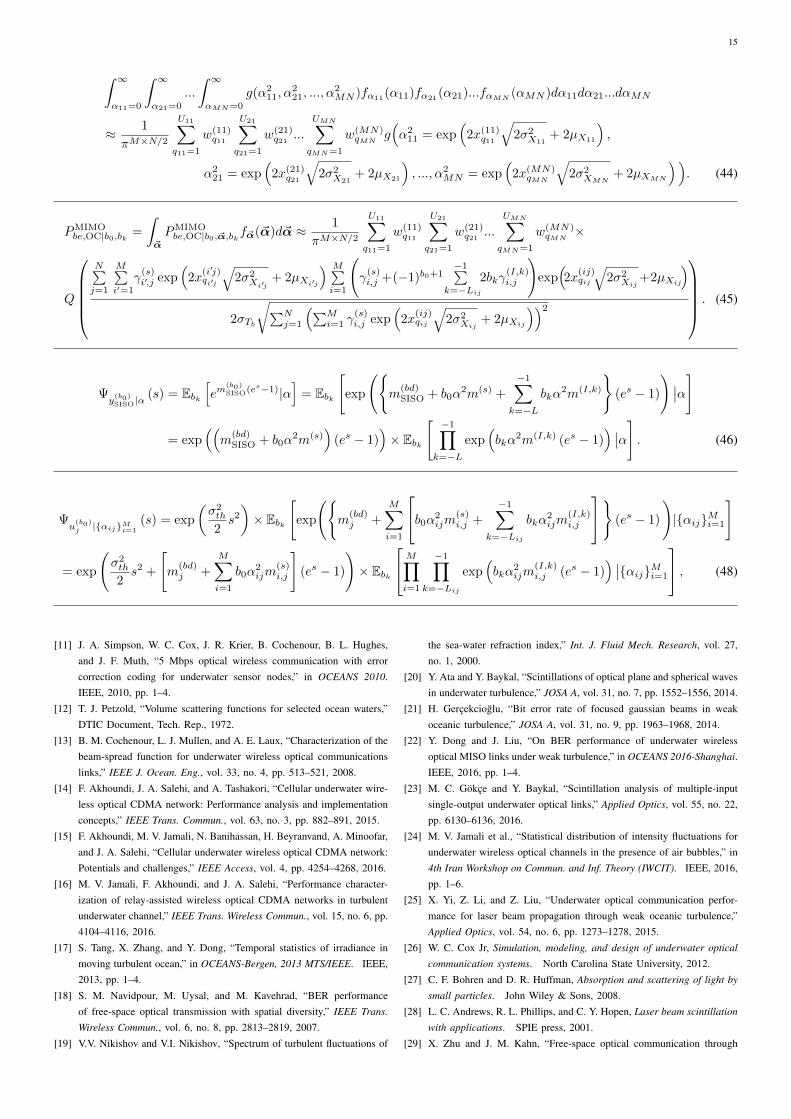
15
∫ ∞α11=0
∫ ∞α21=0
...
∫ ∞αMN=0
g(α211, α
221, ..., α
2MN )fα11
(α11)fα21(α21)...fαMN
(αMN )dα11dα21...dαMN
≈ 1
πM×N/2
U11∑q11=1
w(11)q11
U21∑q21=1
w(21)q21 ...
UMN∑qMN=1
w(MN)qMN
g(α211 = exp
(2x(11)q11
√2σ2
X11+ 2µX11
),
α221 = exp
(2x(21)q21
√2σ2
X21+ 2µX21
), ..., α2
MN = exp(
2x(MN)qMN
√2σ2
XMN+ 2µXMN
)). (44)
PMIMObe,OC|b0,bk =
∫~α
PMIMObe,OC|b0,~α,bkf~α(~α)d~α ≈ 1
πM×N/2
U11∑q11=1
w(11)q11
U21∑q21=1
w(21)q21 ...
UMN∑qMN=1
w(MN)qMN
×
Q
N∑j=1
M∑i′=1
γ(s)i′,j exp
(2x
(i′j)qi′j
√2σ2
Xi′j+ 2µXi′j
) M∑i=1
(γ(s)i,j +(−1)b0+1
−1∑k=−Lij
2bkγ(I,k)i,j
)exp(2x
(ij)qij
√2σ2
Xij+2µXij
)2σTb
√∑Nj=1
(∑Mi=1 γ
(s)i,j exp
(2x
(ij)qij
√2σ2
Xij+ 2µXij
))2 . (45)
Ψy(b0)
SISO|α(s) = Ebk
[em
(b0)
SISO(es−1)|α]
= Ebk
[exp
(m
(bd)SISO + b0α
2m(s) +
−1∑k=−L
bkα2m(I,k)
(es − 1)
)∣∣α]
= exp((m
(bd)SISO + b0α
2m(s))
(es − 1))× Ebk
[ −1∏k=−L
exp(bkα
2m(I,k) (es − 1)) ∣∣α] . (46)
Ψu(b0)j |αijMi=1
(s) = exp
(σ2th
2s2)× Ebk
[exp
(m
(bd)j +
M∑i=1
b0α2ijm
(s)i,j +
−1∑k=−Lij
bkα2ijm
(I,k)i,j
(es − 1)
)|αijMi=1
]
= exp
(σ2th
2s2 +
[m
(bd)j +
M∑i=1
b0α2ijm
(s)i,j
](es − 1)
)× Ebk
M∏i=1
−1∏k=−Lij
exp(bkα
2ijm
(I,k)i,j (es − 1)
) ∣∣αijMi=1
, (48)
[11] J. A. Simpson, W. C. Cox, J. R. Krier, B. Cochenour, B. L. Hughes,and J. F. Muth, “5 Mbps optical wireless communication with errorcorrection coding for underwater sensor nodes,” in OCEANS 2010.IEEE, 2010, pp. 1–4.
[12] T. J. Petzold, “Volume scattering functions for selected ocean waters,”DTIC Document, Tech. Rep., 1972.
[13] B. M. Cochenour, L. J. Mullen, and A. E. Laux, “Characterization of thebeam-spread function for underwater wireless optical communicationslinks,” IEEE J. Ocean. Eng., vol. 33, no. 4, pp. 513–521, 2008.
[14] F. Akhoundi, J. A. Salehi, and A. Tashakori, “Cellular underwater wire-less optical CDMA network: Performance analysis and implementationconcepts,” IEEE Trans. Commun., vol. 63, no. 3, pp. 882–891, 2015.
[15] F. Akhoundi, M. V. Jamali, N. Banihassan, H. Beyranvand, A. Minoofar,and J. A. Salehi, “Cellular underwater wireless optical CDMA network:Potentials and challenges,” IEEE Access, vol. 4, pp. 4254–4268, 2016.
[16] M. V. Jamali, F. Akhoundi, and J. A. Salehi, “Performance character-ization of relay-assisted wireless optical CDMA networks in turbulentunderwater channel,” IEEE Trans. Wireless Commun., vol. 15, no. 6, pp.4104–4116, 2016.
[17] S. Tang, X. Zhang, and Y. Dong, “Temporal statistics of irradiance inmoving turbulent ocean,” in OCEANS-Bergen, 2013 MTS/IEEE. IEEE,2013, pp. 1–4.
[18] S. M. Navidpour, M. Uysal, and M. Kavehrad, “BER performanceof free-space optical transmission with spatial diversity,” IEEE Trans.
Wireless Commun., vol. 6, no. 8, pp. 2813–2819, 2007.
[19] V.V. Nikishov and V.I. Nikishov, “Spectrum of turbulent fluctuations of
the sea-water refraction index,” Int. J. Fluid Mech. Research, vol. 27,no. 1, 2000.
[20] Y. Ata and Y. Baykal, “Scintillations of optical plane and spherical wavesin underwater turbulence,” JOSA A, vol. 31, no. 7, pp. 1552–1556, 2014.
[21] H. Gercekcioglu, “Bit error rate of focused gaussian beams in weakoceanic turbulence,” JOSA A, vol. 31, no. 9, pp. 1963–1968, 2014.
[22] Y. Dong and J. Liu, “On BER performance of underwater wirelessoptical MISO links under weak turbulence,” in OCEANS 2016-Shanghai.IEEE, 2016, pp. 1–4.
[23] M. C. Gokce and Y. Baykal, “Scintillation analysis of multiple-inputsingle-output underwater optical links,” Applied Optics, vol. 55, no. 22,pp. 6130–6136, 2016.
[24] M. V. Jamali et al., “Statistical distribution of intensity fluctuations forunderwater wireless optical channels in the presence of air bubbles,” in4th Iran Workshop on Commun. and Inf. Theory (IWCIT). IEEE, 2016,pp. 1–6.
[25] X. Yi, Z. Li, and Z. Liu, “Underwater optical communication perfor-mance for laser beam propagation through weak oceanic turbulence,”Applied Optics, vol. 54, no. 6, pp. 1273–1278, 2015.
[26] W. C. Cox Jr, Simulation, modeling, and design of underwater optical
communication systems. North Carolina State University, 2012.
[27] C. F. Bohren and D. R. Huffman, Absorption and scattering of light by
small particles. John Wiley & Sons, 2008.
[28] L. C. Andrews, R. L. Phillips, and C. Y. Hopen, Laser beam scintillation
with applications. SPIE press, 2001.
[29] X. Zhu and J. M. Kahn, “Free-space optical communication through

16
atmospheric turbulence channels,” IEEE Trans. Commun., vol. 50, no. 8,pp. 1293–1300, 2002.
[30] T. A. Tsiftsis, H. G. Sandalidis, G. K. Karagiannidis, and M. Uysal,“Optical wireless links with spatial diversity over strong atmosphericturbulence channels,” IEEE Trans. Wireless Commun., vol. 8, no. 2, pp.951–957, 2009.
[31] M. Karimi and M. Nasiri-Kenari, “BER analysis of cooperative systemsin free-space optical networks,” J. Lightw. Technol., vol. 27, no. 24, pp.5639–5647, 2009.
[32] M. Karimi and M. Nasiri-Kenari, “Free space optical communicationsvia optical amplify-and-forward relaying,” J. Lightw. Technol., vol. 29,no. 2, pp. 242–248, 2011.
[33] M. Safari and M. Uysal, “Relay-assisted free-space optical communica-tion,” IEEE Trans. Wireless Commun., vol. 7, no. 12, pp. 5441–5449,2008.
[34] E. J. Lee and V. W. Chan, “Part 1: Optical communication over the clearturbulent atmospheric channel using diversity,” IEEE J. Select Areas
Commun., vol. 22, no. 9, pp. 1896–1906, 2004.[35] M. V. Jamali and J. A. Salehi, “On the BER of multiple-input multiple-
output underwater wireless optical communication systems,” in 4th
International Workshop on Optical Wireless Communications (IWOW).IEEE, 2015, pp. 26–30.
[36] G. Einarsson, Principles of Lightwave Communications. New York:Wiley, 1996.
[37] M. Abramowitz and I. A. Stegun, Handbook of mathematical functions:
with formulas, graphs, and mathematical tables. Courier Corporation,1970.
[38] L. Fenton, “The sum of log-normal probability distributions in scattertransmission systems,” Communications Systems, IRE Transactions on,vol. 8, no. 1, pp. 57–67, 1960.
[39] M. Jazayerifar and J. A. Salehi, “Atmospheric optical CDMA commu-nication systems via optical orthogonal codes,” IEEE Trans. Commun.,vol. 54, no. 9, pp. 1614–1623, 2006.
[40] J. W. Giles and I. N. Bankman, “Underwater optical communicationssystems. part 2: basic design considerations,” in Military Communica-
tions Conference, 2005. MILCOM 2005. IEEE. IEEE, 2005, pp. 1700–1705.
[41] C. Abou-Rjeily and A. Slim, “Cooperative diversity for free-spaceoptical communications: transceiver design and performance analysis,”IEEE Trans. Commun., vol. 59, no. 3, pp. 658–663, 2011.
Mohammad Vahid Jamali was born in Talesh, Iran,on May 22, 1991. He received the B.Sc. degreefrom K.N. Toosi University of Technology, Tehran,Iran, in 2013, and the M.Sc. degree from SharifUniversity of Technology (SUT), Tehran, Iran, in2015, both with honors and in Electrical Engineer-ing. Since 2013, he has been a member of thetechnical staff of the Optical Networks Research Lab(ONRL) at SUT. His general research interests are incommunications theory and optics with emphasis onwireless applications. Specific research areas include
underwater wireless optical communications, mode-division multiplexing inoptical fibers, free-space optics, visible light communications, simultaneouswireless information and power transfer, metamaterials and metasurfaces, andDNA sequencing based on optical computing.
Jawad A. Salehi (M’84-SM’07-FM’10) was bornin Kazemain, Iraq, on December 22, 1956. Hereceived the B.Sc. degree from the University ofCalifornia, Irvine, in 1979, and the M.Sc. and Ph.D.degrees from the University of Southern California(USC), Los Angeles, in 1980 and 1984, respec-tively, all in electrical engineering. He is currentlya Full Professor at the Optical Networks ResearchLaboratory (ONRL), Department of Electrical En-gineering, Sharif University of Technology (SUT),Tehran, Iran. From 1981 to 1984, he was a Full-
Time Research Assistant at the Communication Science Institute, USC. From1984 to 1993, he was a Member of Technical Staff of the Applied ResearchArea, Bell Communications Research (Bellcore), Morristown, NJ. Prof. Salehiwas an Associate Editor for Optical CDMA of the IEEE Transactions onCommunications, since 2001 to 2012. He is among the 250 preeminentand most influential researchers worldwide in the Institute for ScientificInformation (ISI) Highly Cited in the Computer-Science Category.
Farhad Akhoundi received the B.Sc. degree (first-class honor) from Shahid Rajaee Teacher TrainingUniversity (SRTTU), Tehran, in 2010, and the M.Sc.degree from Sharif University of Technology (SUT),Tehran, Iran, in 2012, both in electrical engineering.From 2012 to 2014, he was a member of thetechnical staff of the Optical Networks ResearchLaboratory (ONRL) at SUT. From 2014 to 2015,he was employed by DNA Microarray Analysis Lab(DMA Lab), a knowledge-based company in SUT,working on camera-based DNA microarray scanner.
Farhad is currently working toward the Ph.D. degree in the University ofArizona (UA), Tucson, USA. He is also a Full-Time Graduate ResearchAssistant at College of Optical Sciences, UA. His research interests arein the areas of fiber optics, visible light, and underwater wireless opticalmultiple access networks. He is also interested in multi-photon microscopyand fluorescence imaging in the biosciences.