periodic polya urns, the density method and asymptotics of
TRANSCRIPT
The Annals of Probability2020, Vol. 48, No. 4, 1921–1965https://doi.org/10.1214/19-AOP1411© Institute of Mathematical Statistics, 2020
PERIODIC PÓLYA URNS, THE DENSITY METHOD AND ASYMPTOTICSOF YOUNG TABLEAUX
BY CYRIL BANDERIER1, PHILIPPE MARCHAL2 AND MICHAEL WALLNER3
1LIPN, Université Paris Nord, [email protected], Université Paris Nord, [email protected]
3LaBRI, Université de Bordeaux, [email protected]
Pólya urns are urns where at each unit of time a ball is drawn and re-placed with some other balls according to its colour. We introduce a moregeneral model: the replacement rule depends on the colour of the drawn balland the value of the time (modp). We extend the work of Flajolet et al.on Pólya urns: the generating function encoding the evolution of the urn isstudied by methods of analytic combinatorics. We show that the initial par-tial differential equations lead to ordinary linear differential equations whichare related to hypergeometric functions (giving the exact state of the urns attime n). When the time goes to infinity, we prove that these periodic Pólyaurns have asymptotic fluctuations which are described by a product of gen-eralized gamma distributions. With the additional help of what we call thedensity method (a method which offers access to enumeration and randomgeneration of poset structures), we prove that the law of the southeast cornerof a triangular Young tableau follows asymptotically a product of generalizedgamma distributions. This allows us to tackle some questions related to thecontinuous limit of random Young tableaux and links with random surfaces.
CONTENTS
1. Introduction . . . . . . . . . . . . . . . . . . . . . . . . . . . . . . . . . . . . . . . . . . . . . . . . . . . 19221.1. Periodic Pólya urns . . . . . . . . . . . . . . . . . . . . . . . . . . . . . . . . . . . . . . . . . . . . 19221.2. The generalized gamma product distribution . . . . . . . . . . . . . . . . . . . . . . . . . . . . . . 19231.3. Plan of the article . . . . . . . . . . . . . . . . . . . . . . . . . . . . . . . . . . . . . . . . . . . . . 1926
2. A functional equation for periodic Pólya urns . . . . . . . . . . . . . . . . . . . . . . . . . . . . . . . . 19262.1. Urn histories and differential operators . . . . . . . . . . . . . . . . . . . . . . . . . . . . . . . . . 19262.2. D-finiteness of history generating functions . . . . . . . . . . . . . . . . . . . . . . . . . . . . . . . 1928
3. Moments of periodic Pólya urns . . . . . . . . . . . . . . . . . . . . . . . . . . . . . . . . . . . . . . . . 19303.1. Number of histories: A hypergeometric closed form . . . . . . . . . . . . . . . . . . . . . . . . . . 19303.2. Mean and critical exponent . . . . . . . . . . . . . . . . . . . . . . . . . . . . . . . . . . . . . . . . 19313.3. Higher moments . . . . . . . . . . . . . . . . . . . . . . . . . . . . . . . . . . . . . . . . . . . . . . 19333.4. Limit distribution for periodic Pólya urns . . . . . . . . . . . . . . . . . . . . . . . . . . . . . . . . 1935
4. Urns, trees and Young tableaux . . . . . . . . . . . . . . . . . . . . . . . . . . . . . . . . . . . . . . . . 19374.1. The link between Young tableaux and trees . . . . . . . . . . . . . . . . . . . . . . . . . . . . . . . 19404.2. The density method for Young tableaux . . . . . . . . . . . . . . . . . . . . . . . . . . . . . . . . . 19414.3. The density method for trees . . . . . . . . . . . . . . . . . . . . . . . . . . . . . . . . . . . . . . . 19444.4. The link between trees and urns . . . . . . . . . . . . . . . . . . . . . . . . . . . . . . . . . . . . . 1948
5. Random Young tableaux and random surfaces . . . . . . . . . . . . . . . . . . . . . . . . . . . . . . . . 19535.1. Random surfaces . . . . . . . . . . . . . . . . . . . . . . . . . . . . . . . . . . . . . . . . . . . . . 19535.2. From microscopic to macroscopic models: Universality of the tails . . . . . . . . . . . . . . . . . . 19565.3. Factorizations of gamma distributions . . . . . . . . . . . . . . . . . . . . . . . . . . . . . . . . . . 1958
6. Conclusion and further work . . . . . . . . . . . . . . . . . . . . . . . . . . . . . . . . . . . . . . . . . . 1961Acknowledgements . . . . . . . . . . . . . . . . . . . . . . . . . . . . . . . . . . . . . . . . . . . . . . . . 1961References . . . . . . . . . . . . . . . . . . . . . . . . . . . . . . . . . . . . . . . . . . . . . . . . . . . . . 1962
Received March 2019; revised October 2019.MSC2010 subject classifications. Primary 60C05; secondary 05A15, 60F05, 60K99.Key words and phrases. Pólya urn, Young tableau, generating functions, analytic combinatorics, pumping mo-
ment, D-finite function, hypergeometric function, generalized gamma distribution, Mittag-Leffler distribution.
1921

1922 C. BANDERIER, P. MARCHAL AND M. WALLNER
1. Introduction.
1.1. Periodic Pólya urns. Pólya urns were introduced in a simplified version by GeorgePólya and his PhD student, Florian Eggenberger, in [26, 27, 74], with applications to diseasespreading and conflagrations. They constitute a powerful model, which regularly finds newapplications; see, for example, Rivest’s recent work on auditing elections [78], or the analysisof deanonymization in Bitcoin’s peer-to-peer network [29]. They are well-studied objects incombinatorial and probabilistic literature [6, 31, 62], because they offer fascinatingly richlinks with numerous objects like random recursive trees, m-ary search trees and branchingrandom walks (see, e.g., [7, 22, 43, 44]). In this paper, we introduce a variation which leadsto new links with another important combinatorial structure: Young tableaux. What is more,we solve the enumeration problem of this new Pólya urn model, derive the limit law for theevolution of the urn and give some applications to Young tableaux.
In the Pólya urn model, one starts with an urn with b0 black balls and w0 white balls attime 0. At every discrete time step, one ball is drawn uniformly at random. After inspectingits colour, this ball is returned to the urn. If the ball is black, a black balls and b white ballsare added; if the ball is white, c black balls and d white balls are added (where a, b, c, d ∈N
are nonnegative integers). This process can be described by the so-called replacement matrix:
M =(a b
c d
), a, b, c, d ∈N.
We call an urn and its associated replacement matrix balanced if a + b = c + d . In otherwords, in every step the same number of balls is added to the urn. This results in a determin-istic number of balls after n steps: b0 + w0 + (a + b)n balls.
Now, we introduce a more general model which has rich combinatorial, probabilistic andanalytic properties.
DEFINITION 1.1. A periodic Pólya urn of period p with replacement matrices M1,M2,
. . . ,Mp is a variant of a Pólya urn in which the replacement matrix Mk is used at steps np+k.Such a model is called balanced if each of its replacement matrices is balanced.
For p = 1, this model reduces to the classical Pólya urn model with one replacement ma-trix. In this article, we illustrate the aforementioned rich properties via the following model.
DEFINITION 1.2. Let p,� ∈N. We call a Young–Pólya urn of period p and parameter �
the periodic Pólya urn of period p (with b0 ≥ 1 to avoid degenerate cases) and replacementmatrices
M1 = M2 = · · · = Mp−1 =(
1 00 1
)and Mp =
(1 �
0 1 + �
).
EXAMPLE 1.3. Consider a Young–Pólya urn with parameters p = 2, � = 1, and initialconditions b0 = w0 = 1. The replacement matrices are M1 := ( 1 0
0 1
)for every odd step, and
M2 := ( 1 10 2
)for every even step. This case was analysed by the authors in the extended
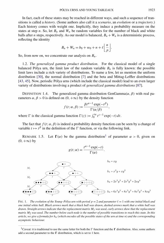
abstract [9]. In the sequel, we will use it as a running example to explain our results.Let us illustrate the evolution of this urn in Figure 1. Each node of the tree corresponds
to the current composition of the urn (number of black balls, number of white balls). Onestarts with b0 = 1 black ball and w0 = 1 white. In the first step, the matrix M1 is used andleads to two different compositions. In the second step, matrix M2 is used, in the third step,matrix M1 is used again, in the fourth step, matrix M2, etc. Thus, the possible compositionsare (2,1) and (1,2) at time 1, (3,2), (2,3) and (1,4) at time 2, (4,2), (3,3), (2,4) and (1,5)
at time 3.
PÓLYA URNS AND YOUNG TABLEAUX 1923
In fact, each of these states may be reached in different ways, and such a sequence of tran-sitions is called a history. (Some authors also call it a scenario, an evolution or a trajectory.)Each history comes with weight one. Implicitly, they induce a probability measure on thestates at step n. So, let Bn and Wn be random variables for the number of black and whiteballs after n steps, respectively. As our model is balanced, Bn +Wn is a deterministic process,reflecting the identity
Bn + Wn = b0 + w0 + n + �
⌊n
p
⌋.
So, from now on, we concentrate our analysis on Bn.
1.2. The generalized gamma product distribution. For the classical model of a singlebalanced Pólya urn, the limit law of the random variable Bn is fully known: the possiblelimit laws include a rich variety of distributions. To name a few, let us mention the uniformdistribution [30], the normal distribution [7] and the beta and Mittag-Leffler distributions[43, 45]. Now, periodic Pólya urns (which include the classical model) lead to an even largervariety of distributions involving a product of generalized gamma distributions [87].
DEFINITION 1.4. The generalized gamma distribution GenGamma(α,β) with real pa-rameters α,β > 0 is defined on (0,+∞) by the density function
f (t;α,β) := βtα−1 exp(−tβ)
�(α/β),
where � is the classical gamma function �(z) := ∫ ∞0 tz−1 exp(−t) dt .
The fact that f (t;α,β) is indeed a probability density function can be seen by a change ofvariable t �→ tβ in the definition of the � function, or via the following link.
REMARK 1.5. Let �(α) be the gamma distribution1 of parameter α > 0, given on(0,+∞) by
g(t;α) = tα−1 exp(−t)
�(α).
FIG. 1. The evolution of the Young–Pólya urn with period p = 2 and parameter � = 1 with one initial black andone initial white ball. Black arrows mark that a black ball was drawn, dashed arrows mark that a white ball wasdrawn. Straight arrows indicate that the replacement matrix M1 was used, curly arrows show that the replacementmatrix M2 was used. The number below each node is the number of possible transitions to reach this state. In thisarticle, we give a formula for hn (which encodes all the possible states of the urn at time n) and the correspondingasymptotic behaviour.
1Caveat: it is traditional to use the same letter for both the � function and the � distribution. Also, some authorsadd a second parameter to the � distribution, which is set to 1 here.
1924 C. BANDERIER, P. MARCHAL AND M. WALLNER
Then one has �(α)L= GenGamma(α,1), and for r > 0, the distribution of the r th power of a
random variable distributed according to �(α) is
�(α)rL= GenGamma(α/r,1/r).
The limit distribution of our urn models is then expressed as a product of such generalizedgamma distributions. We prove in Theorem 3.8 a more general version of the following.
THEOREM 1.6 (The generalized gamma product distribution GenGammaProd for Young–Pólya urns). The renormalized distribution of black balls in a Young–Pólya urn of period p
and parameter � is asymptotically for n → ∞ given by the following product of distributions:
(1)pδ
p + �
Bn
nδ
L−→ Beta(b0,w0)
�−1∏i=0
GenGamma(b0 + w0 + p + i, p + �),
with δ = p/(p + �), and Beta(b0,w0) = 1 when w0 = 0 or Beta(b0,w0) is the beta distribu-tion with support [0,1] and density �(b0+w0)
�(b0)�(w0)xb0−1(1 − x)w0−1 otherwise.
In the sequel, we call this distribution the generalized gamma product distribution anddenote it by GenGammaProd(p, �, b0,w0). We will see in Section 3 that this distribution ischaracterized by its moments, which have a nice factorial shape given in formula (20).
EXAMPLE 1.7. In the case of the Young–Pólya urn with p = 2, � = 1, and w0 = b0 = 1,one has δ = 2/3. Thus, the previous result shows that the number of black balls converges inlaw to a generalized gamma distribution:
22/3
3
Bn
n2/3L−→ Unif(0,1) · GenGamma(4,3) = GenGamma(1,3).
See Section 5.3 and [24], Proposition 4.2, for more identities of this type.
REMARK 1.8 (Period one). When p = 1, our results recover a classical (nonperiodic)urn behaviour. By [45], Theorem 1.3, the renormalization for the limit distribution of Bn inan urn with replacement matrix
( 1 �0 1+�
)is equal to n−1/(1+�). For � = 0 the limit distribution
is the uniform distribution, whereas for � = 1 it is a Mittag-Leffler distribution (see [45],Example 3.1, [30], Example 7), and even simplifies to a half-normal distribution2 when b0 =w0 = 1. Thus, the added periodicity by using this replacement matrix only every pth roundand otherwise Pólya’s replacement matrix
( 1 00 1
)changes the renormalization to n−p/(p+�).
The rescaling factor n−δ with δ = p/(p + �) on the left-hand side of (1) can also beobtained via a martingale computation. The true challenge is to get exact enumeration andthe limit law. It is interesting that there exist other families of urn models exhibiting the samerescaling factor, however, these alternative models lead to different limit laws.
• A first natural alternative model consists in averaging the p replacement matrices. Thisleads to a classical triangular Pólya urn model. The asymptotics is then
Bn
nδ
L−→ B,(2)
2See [93] for other occurrences of the half-normal distribution in combinatorics.

PÓLYA URNS AND YOUNG TABLEAUX 1925
FIG. 2. Left: 20 simulations (drawn in red) of the evolution of Bn, the number of black balls in the Young–Pólyaurn with period p = 2 and parameter � = 1 (first 10,000 steps, with initially b0 = 1 black and w0 = 1 whiteballs), and the mean E(Bn) (drawn in blue). Right: the average (in red) of the 20 simulations, fitting neatly(almost indistinguishable!) the limit curve E(Bn) = �(n2/3) (in blue).
where the distribution of B is, for example, analysed by Flajolet et al. [30] via an ana-lytic combinatorics approach, or by Janson [45] and Chauvin et al. [22] via a probabilisticapproach relying on a continuous-time embedding introduced by Athreya and Karlin [5].For example, averaging the Young–Pólya urn with p = 2, � = 1 and b0 = w0 = 1 leadsto the replacement matrix
( 1 1/20 3/2
). The corresponding classical urn model leads to a limit
distribution with moments given, for example, by Janson in [45], Theorem 1.7:
E(Br) = �(4/3)r!
�(2r/3 + 4/3).
Comparing these moments with the moments of our distribution (equation (20) hereafter)proves that these two distributions are distinct. However, it is noteworthy that they havesimilar tails: we discuss this universality phenomenon in Section 5.2.
• Another interesting alternative model, called multi-drawing Pólya urn model, consists indrawing multiple balls at once; see Lasmar et al. [58] or Kuba and Sulzbach [56]. Groupingp units of time into one drawing leads to a new replacement matrix. For example, for p = 2and � = 1 we can approximate a Young–Pólya urn by an urn where at each unit of time 2balls are drawn uniformly at random. If both of them are black we add 2 black balls and 1white ball, if one is black and one is white we add 1 black and 2 white ball, and if both ofthem are white we add 3 white balls. Then the same convergence as in equation (2) holds,yet again with a different limit distribution, as can be seen by comparing the means andvariances; compare Kuba and Mahmoud [54], Theorem 1, with our Example 3.7.
For all these alternative models, the corresponding histories are inherently different: noneof them gives the exact generating function of periodic Pólya urns nor gives the closed formof the underlying distribution. This also motivates the exact and asymptotic analysis of ourperiodic model, which therefore enriches the urn world with new special functions.
Figure 2 shows that the distribution of Bn is spread; this is consistent with our result that thestandard deviation and the mean E(Bn) (drawn in blue) have the same order of magnitude.3
The fluctuations around this mean are given by the generalized gamma product limit law fromequation (1), as proven in Section 3. Let us first mention some articles where this distributionhas already appeared before:
3The classical urn models with replacement matrices being either M1 or M2 also have such a spread; see [30],Figure 1.

1926 C. BANDERIER, P. MARCHAL AND M. WALLNER
• in Janson [47], as an instance of distributions with moments of gamma type, like the dis-tributions occurring for the area of the supremum process of the Brownian motion;
• in Peköz, Röllin and Ross [70], as distributions of processes on walks, trees, urns andpreferential attachments in graphs, where these authors also consider what they call a Pólyaurn with immigration, which is a special case of a periodic Pólya urn (other models orrandom graphs have these distributions as limit laws [19, 84]);
• in Khodabin and Ahmadabadi [53] following a tradition to generalize special functions byadding parameters in order to capture several probability distributions, such as, for exam-ple, the normal, Rayleigh and half-normal distribution, as well as the MeijerG function (seealso the addendum of [47], mentioning a dozen other generalizations of special functions).
1.3. Plan of the article. Our main results are the explicit enumeration results and linkswith hypergeometric functions (Theorems 2.3 and 3.1), and the limit law involving a prod-uct of generalized gamma distributions (Theorem 3.8, or the simplified version of it givenfor readability in Theorem 1.6 above). It is a nice cherry on the cake that this limit law alsodescribes the fluctuations of the southeast4 corner of a random triangular Young tableau (asproven in Theorem 4.23). We believe that the methods used, that is, the generating functionsfor urns (developed in Section 2), the way to access the moments (developed in Section 3),and the density method for Young tableaux (developed in Section 4) are an original combi-nation of tools, which should find many other applications in the future. Finally, Section 5gives a relation between the southeast and the northwest corners of triangular Young tableaux(Proposition 5.7) and a link with factorizations of gamma distributions. Additionally, we dis-cuss some universality properties of random surfaces, and we show to what extent the tailsof our distributions are related to the tails of Mittag-Leffler distributions (Theorem 5.3), andwhen they are sub-Gaussian (Proposition 5.6).
In the next section, we translate the evolution of the urn into the language of generatingfunctions by encoding the dynamics of this process into partial differential equations.
2. A functional equation for periodic Pólya urns.
2.1. Urn histories and differential operators. Let hn,b,w be the number of histories of aperiodic Pólya urn after n steps with b black balls and w white balls, with an initial state ofb0 black and w0 white balls. We define the polynomials
hn(x, y) := ∑b,w≥0
hn,b,wxbyw.
Note that these are indeed polynomials as there is just a finite number of histories after n
steps. Due to the balanced urn model these polynomials are homogeneous. We collect allthese histories in the trivariate exponential generating function
H(x,y, z) := ∑n≥0
hn(x, y)zn
n! .
EXAMPLE 2.1. For the Young–Pólya urn with p = 2, � = 1, and b0 = w0 = 1, we getfor the first three terms of H(x,y, z) the expansion (compare Figure 1)
H(x,y, z) = xy + (xy2 + x2y
)z + (
2xy4 + 2x2y3 + 2x3y2)z2
2+ · · · .
4In this article, we use the French convention to draw the Young tableaux; see Section 4 and [61].

PÓLYA URNS AND YOUNG TABLEAUX 1927
In this section, our goal is to derive a partial differential equation describing the evolutionof the periodic Pólya urn model.
The periodic nature of the problem motivates to split the number of histories into p residueclasses. Let H0(x, y, z),H1(x, y, z), . . . ,Hp−1(x, y, z) be the generating functions of histo-ries after 0,1, . . . , p − 1 draws modulo p, respectively. In particular, we have
Hi(x, y, z) := ∑n≥0
hpn+i (x, y)zpn+i
(pn + i)! ,
for i = 0,1, . . . , p − 1 such that
H(x,y, z) = H0(x, y, z) + H1(x, y, z) + · · · + Hp−1(x, y, z).
Next, we associate with the two distinct replacement matrices(1 00 1
)and
(1 �
0 1 + �
)
from Definition 1.2 the differential operators D1 and D2, respectively. We get
D1 := x2∂x + y2∂y and D2 := y�D1,
where ∂x and ∂y are defined as the partial derivatives ∂∂x
and ∂∂y
, respectively. This models
the evolution of the urn. For example, in the term x2∂x , the derivative ∂x represents drawinga black ball and the multiplication by x2 returning this black ball and an additional black ballinto the urn. The other terms have analogous interpretations.
With these operators, we are able to link the consecutive drawings with the followingsystem:
(3)
{∂zHi+1(x, y, z) = D1Hi(x, y, z) for i = 0,1, . . . , p − 2,
∂zH0(x, y, z) = D2Hp−1(x, y, z).
Note that the derivative ∂z models the evolution in time. We see two types of transitions:in the first p − 1 rounds the urn behaves like a normal Pólya urn, but in the pth round weadditionally add � white balls. The first transition type is modelled by the D1 operator andthe second type by the D2 operator. This system of partial differential equations naturallycorresponds to recurrences on the level of coefficients hn,b,w , and vice versa. This philosophyis well explained in the symbolic method part of [33] (see also [30, 31, 42, 67] for examplesof applications to urns).
As a next step, we want to eliminate the y variable in these equations. This is possible asthe number of balls in each round and the number of black and white balls are connected dueto the fact that we are dealing with balanced urns. As observed previously, one has
(4) number of balls after n steps = s0 + n + �
⌊n
p
⌋,
with s0 := b0 + w0 being the number of initial balls. Therefore, for any xbywzn appearing inH(x,y, z), we have
b + w = s0 + n + �n − i
pif n ≡ i mod p,
which directly translates into the following system of equations (for i = 0, . . . , p − 1):
(5) x∂xHi(x, y, z) + y∂yHi(x, y, z) =(
1 + �
p
)z∂zHi(x, y, z) +
(s0 − i�
p
)Hi(x, y, z).

1928 C. BANDERIER, P. MARCHAL AND M. WALLNER
These equations are contractions in the metric space of formal power series in z (see, e.g., [8]or [33], Section A.5), so, given the initial conditions [z0]Hi(x, y, z), the Banach fixed-pointtheorem entails that this system has a unique solution: our set of generating functions. Now,because of the deterministic link between the number of black balls and the number of whiteballs, it is natural to introduce the two shorthands H(x, z) := H(x,1, z) and Hi(x, z) :=Hi(x,1, z). What is the nature of these functions? This is what we tackle now.
2.2. D-finiteness of history generating functions. Let us first give a formal definition ofthe fundamental concept of D-finiteness.
DEFINITION 2.2 (D-finiteness). A power series F(z) = ∑n≥0 fnz
n with coefficients insome ring A is called D-finite if it satisfies a linear differential equation L.F (z) = 0, whereL �= 0 is a differential operator, L ∈ A[z, ∂z]. Equivalently, the sequence (fn)n∈N is calledP-recursive: it satisfies a linear recurrence with polynomial coefficients in n. Such functionsand sequences are also sometimes called holonomic.
D-finite functions are ubiquitous in combinatorics, computer science, probability theory,number theory, physics, etc.; see, for example, [1] or [33], Appendix B.4. They possess clo-sure properties galore; this provides an ideal framework for handling (via computer algebra)sums and integrals involving such functions [15, 71]. The same idea applies to a full familyof linear operators (differentiations, recurrences, finite differences, q-shifts) and is unifiedby what is called holonomy theory. This theory leads to a fascinating algorithmic universeto deal with orthogonal polynomials, Laplace and Mellin transforms, and most of the inte-grals of special functions: it offers powerful tools to prove identities, asymptotic expansions,numerical values, structural properties; see [50, 68, 76].
We have seen in Section 2.1 that the dynamics of urns is intrinsically related to partialdifferential equations (mixing ∂x , ∂y , and ∂z). It is therefore a nice surprise that it is alsopossible to describe their evolution in many cases with ordinary differential equations (i.e.,involving only ∂z).
THEOREM 2.3 (Differential equations for histories). The generating functions describ-ing a Young–Pólya urn of period p and parameter � with initially s0 = b0 + w0 balls, whereb0 are black and w0 are white, satisfy the following system of p partial differential equations:
(6) ∂zHi+1(x, z) = x(x − 1)∂xHi(x, z) +(
1 + �
p
)z∂zHi(x, z) +
(s0 − i�
p
)Hi(x, z),
for i = 0, . . . , p − 1 with Hp(x, z) := H0(x, z). Moreover, if any of the corresponding gen-erating functions (ordinary, exponential, ordinary probability or exponential probability) isD-finite in z, then all of them are D-finite in z.
PROOF. First, let us prove the system involving ∂z and ∂x only. Combining (3) and (5),we eliminate ∂y . Then it is legitimate to insert y = 1 as there appears no differentiation withrespect to y anymore. This gives (6).
Now, assume the ordinary generating function is D-finite. Multiplying a holonomic se-quence by n! (or by 1/n!, or more generally by any holonomic sequence) gives a new se-quence, which is also holonomic. In other words, the Hadamard product of two holonomicsequences is still holonomic [89], Chapter 6.4. This proves that the ordinary and exponentialversions of our generating functions H and Hi are D-finite in z.
Finally, for the probability generating function defined as∑n,b,w
P(Bn = b and Wn = w)xbywzn = ∑n
hn(x, y)
hn(1,1)zn,

PÓLYA URNS AND YOUNG TABLEAUX 1929
TABLE 1Size of the D-finite equations for the four types of generating functions of histories (for the urn model of
Example 2.4). We use the abbreviations EGF (exponential generating function), OGF (ordinary generatingfunction), EPGF (exponential probability generating function), OPGF (ordinary probability generating
function). We omit the degree of the variable y, as, for balanced urns, it is trivially related to the degree in x
Type Generating function Order in ∂z Degree in z Degree in x
EGF∑
n,b,w hn,b,wxbyw zn
n! 5 13 16OGF
∑n,b,w hn,b,wxbywzn 7 23 20
EPGF∑
n,b,w P(Bn = b and Wn = w)xbyw zn
n! 8 4 15OPGF
∑n,b,w P(Bn = b and Wn = w)xbywzn 3 13 14
it is in general not the case that it is holonomic if the initial ordinary generating functionis holonomic. But in our case a miracle occurs: in each residue class of n mod p, the se-quence (hpm+i(1,1))m∈N is hypergeometric (as shown in Theorem 3.1), therefore, the p
subsequences (1/hpm+i(1,1))m∈N are also hypergeometric, and thus the above probabil-ity generating function (which is the sum of p holonomic functions, each one being theHadamard product of two holonomic functions) is holonomic. �
Experimentally, in most cases a few terms suffice to guess a holonomic sequence in z.We believe that this sequence is always holonomic, yet we were not able to prove it in fullgenerality. We plan to comment more on this and other related phenomena in a forthcomingarticle.
EXAMPLE 2.4. In the case of the Young–Pólya urn with p = 2, � = 1, and b0 = w0 = 1,the differential equations for histories (6) are⎧⎪⎪⎨
⎪⎪⎩∂zH0(x, z) = x(x − 1)∂xH1(x, z) + 3
2z∂zH1(x, z) + 3
2H1(x, z),
∂zH1(x, z) = x(x − 1)∂xH0(x, z) + 3
2z∂zH0(x, z) + 2H0(x, z).
In addition to this system of partial differential equations, there exist also two ordinarylinear differential equations in z for H0 and H1 and, therefore, for their sum H := H0 + H1,the generating function of all histories.
In Table 1, we compare the size of the D-finite equations5 for the different generatingfunctions. For example, for the ordinary probability generating function one has the equationL.F (x, z) = 0, where L is the following differential operator of order 3 in ∂z:
L = 9z(z − 1)(z + 1)(15x13z10 + · · · + 3
)∂3z + 3
(375x13z12 + · · · − 21
)∂2z
+ 2(1020x13z11 + · · · + 42
)∂z + 600x13z10 + · · · + 1.
The singularity at z = 1 of the leading coefficient reflects the fact that F is a probabilitygenerating function (and thus has radius of convergence equal to 1). It is noteworthy thatsome roots of the indicial polynomial of L at z = 1 differ by an integer, this phenomenonis sometimes called resonance, and often occurs in the world of hypergeometric functions;we will come back to these facts and what they imply for the asymptotics (see also [33],Chapter IX. 7.4).
5When we say the equation, we mean the linear differential equation of minimal order in ∂z, and then minimaldegrees in z and x, up to a constant factor for its leading term.
1930 C. BANDERIER, P. MARCHAL AND M. WALLNER
Note that the fact to be D-finite has an unexpected consequence: it allows a surprisinglyfast computation of hn in time O(
√n log2 n) (see [15], Chapter 15, for a refined complexity
analysis of the corresponding algorithm). Such efficient computations are, for example, im-plemented in the Maple package gfun (see [83]). This package, together with some packagesfor differential elimination (see [16, 35]), allows us to compute the different D-finite equa-tions from Table 1, via the union of our Theorem 3.1 on the hypergeometric closed forms andthe closure properties mentioned above.
Another important consequence of the D-finiteness is that the type of the singularitiesthat the function can have is constrained. In particular, the following important subclass ofD-finite functions can be automatically analysed:
REMARK 2.5. Flajolet and Lafforgue have proven that under some “generic” conditions,such D-finite equations lead to a Gaussian limit law (see [32], Theorem 7, and [33], Chap-ter IX. 7.4). It is interesting that these generic conditions are not fulfilled in our case: we havea cancellation of the leading coefficient of L at (x, z) = (1,1), a confluence for the indicialpolynomial, and the resonance phenomenon mentioned above! The natural model of periodicPólya urns thus leads to an original analytic situation, which offers a new (non-Gaussian)limit law.
We thus need another strategy to determine the limit law. In the next section, we use thesystem of equations (6) to iteratively derive the moments of the distribution of black ballsafter n steps.
3. Moments of periodic Pólya urns. In this section, we give the proof of Theorem 1.6and a generalization of it. As it will use the method of moments, let us introduce mr(n), ther th factorial moment of the distribution of black balls after n steps, that is,
mr(n) := E(Bn(Bn − 1) · · · (Bn − r + 1)
).
Expressing them in terms of the generating function H(x, z), it holds that
mr(n) =[zn] ∂r
∂xr H(x, z)
∣∣∣∣x=1
[zn]H(1, z),
where [zn]∑n fnzn := fn is the coefficient extraction operator.
We will compute the sequences of the numerator and denominator separately. We startwith the denominators, the total number of histories after n steps.
3.1. Number of histories: A hypergeometric closed form. We prove that H(1, z) satisfiesa miraculous property which does not hold for H(x, z): it is a sum of generalized hypergeo-metric functions (see, e.g., [3] for an introduction to this important class of special functions).
THEOREM 3.1 (Hypergeometric closed forms). Let hn := n![zn]H(1, z) be the numberof histories after n steps in a Young–Pólya urn of period p and parameter � with initiallys0 = b0 + w0 balls, where b0 are black and w0 are white. Then, for each i, (hpm+i )m∈N is ahypergeometric sequence, satisfying the recurrence
(7) hp(m+1)+i =i−1∏j=0
((p + �)(m + 1) + s0 + j
)p−1∏j=i
((p + �)m + s0 + j
)hpm+i .
Equivalent closed forms are given in equations (10), (11) and (12).

PÓLYA URNS AND YOUNG TABLEAUX 1931
PROOF. Substituting x = 1 into (6) and extracting the coefficient of zn for i = 0, . . . ,
p − 1 gives the recurrence
hn+1 =((
1 + �
p
)n + bn
)hn with(8)
bn := s0 − �
p(n mod p),(9)
where n mod p gives values in {0,1, . . . , p − 1}. Iterating this recurrence relation p timesgives (7). This leads to the following equivalent closed forms:
hpm+i = (p + �)pm+i∏p−1j=0 �(
s0+jp+�
)
i−1∏j=0
�
(m + 1 + s0 + j
p + �
)p−1∏j=i
�
(m + s0 + j
p + �
),(10)
hpm+i = (p + �)pm �(s0 + (p + �)m + i)
�(s0 + (p + �)m)
p−1∏j=0
�(m + s0+jp+�
)
�(s0+jp+�
).(11)
Accordingly, the function H(1, z) is the sum of p generalized hypergeometric functionspFp−1:
H(1, z) =p−1∑i=0
(s0 + i − 1
i
)zi
pFp−1
(L1(i),L2(i),
((p + l)z
p
)p),(12)
where the lists of arguments are given by L1(i) :=[(
s0+jp+�
+ 1)j=0,...,i−1
,(
s0+jp+�
)j=i,...,p−1
]and L2(i) :=
[(jp
+ 1)j=1,...,i
,(
jp
)j=i+1,...,p−1
]. �
EXAMPLE 3.2. In the case of the Young–Pólya urn with p = 2, � = 1, and b0 = w0 = 1,one has the hypergeometric closed forms for hn := n![zn]H(1, z):
hn =
⎧⎪⎪⎪⎨⎪⎪⎪⎩
3n�(n
2 + 1)�(n2 + 2
3)
�(2/3)if n is even,
3n�(n
2 + 12)�(n
2 + 76)
�(2/3)if n is odd.
Alternatively, this sequence satisfies h(n + 2) = 32h(n + 1) + 1
4(9n2 + 21n + 12)h(n).This sequence was not in the On-Line Encyclopedia of Integer Sequences, accessi-ble at https://oeis.org. We added it there; it is now A293653, and it starts like this:1,2,6,30,180,1440,12960,142560,1710720, . . . . The exponential generating function canbe written as the sum of two hypergeometric functions:
H(1, z) = 2F1
([2
3,1
],
[1
2
],
(3z
2
)2)+ 2z 2F1
([5
3,1
],
[3
2
],
(3z
2
)2).
3.2. Mean and critical exponent. Let us proceed with the computation of moments. Forthis purpose, define
h(r)n := n![zn] ∂r
∂xrH(x, z)
∣∣∣∣x=1
,
as the coefficient of (x−1)r zn
r!n! of H(x, z). Then the r th moment is obviously computed as
mr(n) = h(r)n
hn. The key idea why to use these quantities comes from the differential equations
for histories (6). The derivative of Hi(x, z) with respect to x has a factor (x − 1), which
1932 C. BANDERIER, P. MARCHAL AND M. WALLNER
makes it possible to compute h(r)n iteratively by taking the r-th derivative with respect to x
and substituting x = 1. Let us define the auxiliary functions
H(r)i (z) := ∂r
∂xrHi(x, z)
∣∣∣∣x=1
.
We get for i = 0, . . . , p − 1 (with bi as defined in (9)):
∂zH(r)i+1(z) =
(1 + �
p
)z∂zH
(r)i (z) + (bi + r)H
(r)i (z) + (r − 1)rH
(r−1)i (z).
From this equation we extract the nth coefficient with respect to z and multiply by n! to get
h(r)n+1 =
((1 + �
p
)n + bn + r
)h(r)
n + (r − 1)rh(r−1)n .(13)
We reveal a perturbed version of (8). In particular, this is a nonhomogeneous linear recurrencerelation. Yet, the inhomogeneity only emerges for r ≥ 2. Thus, the mean is derived directlywith the same approach as hn previously. Note that for r = 1, equation (13) is exactly of thesame type as (8) after replacing s0 by s0 + r and h0 by b0. We get without any further work
h(1)pm+i = C1(p + �)pm+i
i−1∏j=0
�
(m + 1 + s0 + 1 + j
p + �
)p−1∏j=i
�
(m + s0 + 1 + j
p + �
),
C1 = b0
p−1∏j=0
�
(s0 + 1 + j
p + �
)−1.
Combining the last two results, we get a (surprisingly) simple expression
EBpm+i = h(1)pm+i
hpm+i
= C1
C0
∏i−1j=0 �(m + 1 + s0+1+j
p+�)∏p−1
j=i �(m + s0+1+jp+�
)∏i−1j=0 �(m + 1 + s0+j
p+�)∏p−1
j=i �(m + s0+jp+�
)
= b0�(
s0p+�
)
�(s0+pp+�
)
(m + s0 + i
p + �
) �(m + s0+pp+�
)
�(m + 1 + s0p+�
).
In particular, it is straightforward to compute an asymptotic expansion for the mean by Stir-ling’s approximation. For i = 0,1, . . . , p − 1, we get
EBpm+i = b0�(
s0p+�
)
�(s0+pp+�
)m
pp+�
(1 + O
(1
m
)).
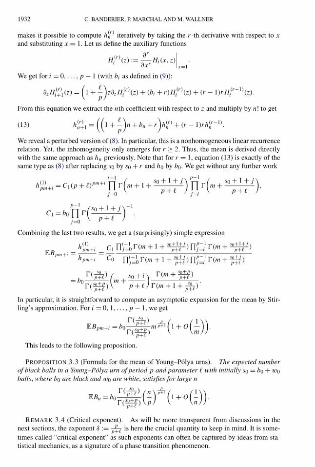
This leads to the following proposition.
PROPOSITION 3.3 (Formula for the mean of Young–Pólya urns). The expected numberof black balls in a Young–Pólya urn of period p and parameter � with initially s0 = b0 + w0balls, where b0 are black and w0 are white, satisfies for large n
EBn = b0�(
s0p+�
)
�(s0+pp+�
)
(n
p
) pp+�
(1 + O
(1
n
)).
REMARK 3.4 (Critical exponent). As will be more transparent from discussions in thenext sections, the exponent δ := p
p+�is here the crucial quantity to keep in mind. It is some-
times called “critical exponent” as such exponents can often be captured by ideas from sta-tistical mechanics, as a signature of a phase transition phenomenon.

PÓLYA URNS AND YOUNG TABLEAUX 1933
EXAMPLE 3.5. For the Young–Pólya urn with p = 2, � = 1, and b0 = w0 = 1, the ex-pected number of black balls at time n is thus
EBn = �(2/3)
�(4/3)
(n
2
) 23(
1 + O
(1
n
))≈ 0.9552n2/3
(1 + O
(1
n
)).
This is coherent with the renormalization used for the limit law of Bn in Example 1.7.
3.3. Higher moments. When computing higher moments, the first idea is to transform thenonhomogeneous recurrence relation (13) into a homogeneous one. To this aim, one rewritesthis equation into
yn+1 − (an + bn + r)yn = (r − 1)rh(r−1)n and y0 = ∂r
xH(x,0)∣∣x=1.(14)
Note that we have yn = h(r)n , the r-th moment we want to determine. From now on, we speak
of the homogeneous equation to refer to the left-hand side of equation (14) set equal to 0,whereas equation (14) itself is called the nonhomogeneous equation. In order to get h
(r)n , we
proceed by induction on r : we assume that the (r − 1)-st moment is known (thus, we knowthe right-hand side of (14)), and we want to express the r th moment h
(r)n (i.e., we want to
solve the recurrence (14) for yn) in terms of this previously computed quantity.As for any linear recurrence, its solution is given by a combination of a solution h
(r)n,hom of
the homogeneous equation and of a particular solution h(r)n,par such that
h(r)n = Crh
(r)n,hom − h(r)
n,par,(15)
with Cr ∈ R such that the initial condition in (14) is satisfied. We will show that asymptot-ically only the solution h
(r)n,hom of the homogeneous equation is dominant. First of all, this
solution is easy to compute, as it is again of the same type as (8). We have
h(r)pm+i,hom = (p + �)pm+i
i−1∏j=0
�
(m + 1 + s0 + r + j
p + �
)p−1∏j=i
�
(m + s0 + r + j
p + �
).(16)
The next idea is to find a particular solution of the nonhomogeneous recurrence relation (14).We will show that the equation exhibits a phenomenon similar to resonance and we will showthat the particular solution is
h(r)n,par =
r−1∑j=1
djh(j)n for constants dj ∈R.(17)
We will compute the coefficients dj by induction from r − 1 to 1. First, we observe that
the inhomogeneous part in the r th equation is a multiple of the solution h(r−1)n of the (r − 1)-
st equation. This motivates us to set yn = h(r−1)n in the homogeneous equation of the r-th
equation. Using (14) then leads to
h(r−1)n+1 − (an + bn + r)h(r−1)
n = (r − 1)(r − 2)h(r−2)n − h(r−1)
n .
Thus, by linearity we choose h(r)n,par = zn − (r − 1)rh
(r−1)n , that is, dr−1 = (r − 1)r , as a first
candidate for a particular solution where zn is (still) an undetermined sequence. Inserting thisinto (14), we get a recurrence relation for zn, where we reduced the order of the inhomogene-ity by one in r (in comparison with (14)):
zn+1 − (an + bn + r)zn = r(r − 1)2(r − 2)h(r−2)n .

1934 C. BANDERIER, P. MARCHAL AND M. WALLNER
Continuing this approach, we compute all dj ’s inductively. As the order in r decreases, thisapproach terminates at r = 1. One thus identifies the constants dj of formula (17):
dj =r∏
i=j+1
(i − 1)i
r − i + 1=
(r − 1j − 1
)r!j ! = L(r, j),
with L(r, j) being the Lah numbers, which express the rising factorials in terms of fallingfactorials6 (see [57] and [77], page 43):
r∑j=1
L(r, j)xj = xr .(18)
Then, by (15) we get the general solution of the r th moment
h(r)n = Crh
(r)n,hom −
r−1∑j=1
L(r, j)h(j)n .(19)
For n = 0, equation (19) becomes
h(r)0 = ∂r
xH(x,0)∣∣x=1 = b0
r = Crh(r)0,hom −
r−1∑j=1
L(r, j)b0j ,
which gives together with (18) that Crh(r)0,hom = b0
r .Finally, we are now able to compute the asymptotic expansion of the r th (factorial) mo-
ment. Using Stirling’s approximation, the quotient of the quantities given by (19) and (16)
gives that h(j)n
h(r)n,hom
= O(n− (r−j)p
p+� ), for j = 1, . . . , r − 1. Hence, for the r th moment given by
(19), we proved that the contribution of h(r)n,hom is the asymptotically dominant one. This leads
to the main result on the asymptotics of the moments.
PROPOSITION 3.6 (Moments of Young–Pólya urns). The r th (factorial) moment of Bn
(the number of black balls in the Young–Pólya urn of period p and parameter � with initiallys0 = b0 + w0 balls, where b0 are black and w0 are white) for large n satisfies6
mr(n) = γrnδr
(1 + O
(1
n
))with γr = b0
r
pδr
p−1∏j=0
�(s0+jp+�
)
�(s0+r+j
p+�)
and δ = p
p + �.
EXAMPLE 3.7. For the Young–Pólya urn with p = 2, � = 1, and b0 = w0 = 1, the vari-ance of the number of black balls at time n is thus
VBn = 27
8
�(23)2(3�(4
3) − �(23)2)
21/3π2 n4/3(
1 + O
(1
n
))≈ 0.42068n4/3
(1 + O
(1
n
)).
NOTA BENE. The reasoning following equation (19) shows that these asymptotics arethe same for the moments and the factorial moments, so in the sequel we refer to this resultindifferently from both points of view.
6The falling factorial xr is defined by xr := x(x − 1) · · · (x − r + 1) = �(x + 1)/�(x − r + 1), while the rising
factorial xr is defined by xr := �(x + r)/�(x) = x(x + 1) · · · (x + r − 1). These two notations were introducedas an alternative to the Pochhammer symbols by Graham, Knuth and Patashnik in [39].

PÓLYA URNS AND YOUNG TABLEAUX 1935
3.4. Limit distribution for periodic Pólya urns. We use the method of moments to proveTheorem 1.6 (the generalized gamma product distribution for Young–Pólya urns). The nat-ural factors occurring in the constant γr of Proposition 3.6, may they be 1/�(
s+r+jp+�
) or
(b0r )1/p/�(
s+r+jp+�
), do not satisfy the determinant/finite difference positivity tests for theStieltjes/Hamburger/Hausdorff moment problems, therefore, no continuous distribution hassuch moments (see [92]). However, the full product does correspond to moments of a dis-tribution which is easier to identify if we start by transforming the constant γr by the Gaussmultiplication formula of the gamma function; this gives
γr = (p + �)r
pδr
�(b0 + r)�(s0)
�(b0)�(s0 + r)
�−1∏j=0
�(s0+r+p+j
p+�)
�(s0+p+j
p+�)
.
Combining this result with the rth (factorial) moment mr(n) from Proposition 3.6, we see
that the moments E(B∗n
r) of the rescaled random variable B∗n := pδ
p+�Bn
nδ converge for n → ∞to the limit
mr := �(b0 + r)�(s0)
�(b0)�(s0 + r)
�−1∏j=0
�(s0+r+p+j
p+�)
�(s0+p+j
p+�)
,(20)
a simple formula involving the parameters (p, �, b0,w0) of the model (with s0 := b0 + w0).Next, note that the following sum diverges (recall that 0 ≤ (1 − δ) < 1):
∑r>0
m−1/(2r)r = ∑
r>0
((p + �)e
r
)(1−δ)/2(1 + o(1)
) = +∞.
Therefore, a result by Carleman (see [21], pages 189–220) implies that there exists a uniquedistribution (let us call it D) with such moments mr . Then, by the limit theorem of Fréchetand Shohat [34], page 536,7 B∗
n converges to D.Finally, we use the shape of the moments in (20) in order to express this distribution D
in terms of the main functions defined in Section 1. First, note that if for some independentrandom variables X, Y , Z, one has E(Xr) = E(Y r)E(Zr) (and if Y and Z are determined by
their moments), then XL= YZ. Therefore, we treat the factors independently. The first factor
corresponds to a beta distribution Beta(b0,w0). For the other factors, it is easy to check thatif X ∼ GenGamma(α,β) is a generalized gamma distributed random variable (as definedin Definition 1.4), then it is a distribution determined by its moments, which are given by
E(Xr) = �(α+rβ
)
�( αβ)
. Therefore, the expression in (20) characterizes the GenGammaProd distri-
bution. This completes the proof of Theorem 1.6.For reasons which would be clear in Section 4, it was natural to focus first on Young–Pólya
urns. However, the method presented is this section allows us to handle more general models.It would have been quite indigestible to present directly the general proof with heavy notationand many variables but now that the reader got the key steps of the method, she should bedelighted to recycle all of this for free in the following much more general result.
THEOREM 3.8 (The generalized gamma product distribution for triangular balanced urns).Let p ≥ 1 and �1, . . . , �p ≥ 0 be nonnegative integers. Consider a periodic Pólya urn of pe-
riod p with replacement matrices M1, . . . ,Mp given by Mj := ( 1 �j
0 1+�j
). Then the renormal-
ized distribution of black balls is asymptotically for n → ∞ given by the following product
7As a funny coincidence, Fréchet and Shohat mention in [34] that the generalized gamma distribution withparameter p ≥ 1/2 is uniquely characterized by its moments.
1936 C. BANDERIER, P. MARCHAL AND M. WALLNER
of distributions:
pδ
p + �
Bn
nδ
L−→ Beta(b0,w0)
p+�−1∏i=1
i �=�1+···+�j+j with 1≤j≤p−1
GenGamma(b0 + w0 + i, p + �)
with � = �1 + · · · + �p , δ = p/(p + �), and Beta(b0,w0) = 1 when w0 = 0.
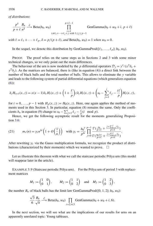
In the sequel, we denote this distribution by GenGammaProd([�1, . . . , �p];b0,w0).
PROOF. The proof relies on the same steps as in Sections 2 and 3 with some minortechnical changes, so we only point out the main differences.
The behaviour of the urn is now modeled by the p differential operators Dj = y�j (x2∂x +y2∂y). As the matrices are balanced, there is (like in equation (4)) a direct link between thenumber of black balls and the total number of balls. This allows to eliminate the y variableand leads to the following system of partial differential equations (which generalizes equation(6)):
∂zHi+1(x, z) = x(x − 1)∂xHi(x, z) +(
1 + �
p
)z∂zHi(x, z) +
(s0 −
i∑j=1
�j − i�
p
)Hi(x, z),
for i = 0, . . . , p − 1 with Hp(x, z) := H0(x, z). Here, one again applies the method of mo-ments used in this Section 3. In particular, equation (8) remains the same. Only the coeffi-cients bn in equation (9) change to s0 − ∑i
j=1 �j − �p(i mod p).
Hence, we get the following asymptotic result for the moments generalizing Proposi-tion 3.6:
mr(n) = γrnδr
(1 + O
(1
n
))with γr = b0
r
pδr
p−1∏j=0
�(s0
p+�+ j+∑j
k=1 �k
p+�)
�(s0+rp+�
+ j+∑jk=1 �k
p+�)
.(21)
After rewriting γr via the Gauss multiplication formula, we recognize the product of distri-butions (characterized by their moments) which we wanted to prove. �
Let us illustrate this theorem with what we call the staircase periodic Pólya urn (this modelwill reappear later in the article).
EXAMPLE 3.9 (Staircase periodic Pólya urn). For the Pólya urn of period 3 with replace-ment matrices
M1 :=(
1 00 1
), M2 :=
(1 10 2
)and M3 :=
(1 20 3
),
the number Bn of black balls has the limit law GenGammaProd([0,1,2];b0,w0):√
3
6
Bn√n
L−→ Beta(b0,w0)∏
i=2,4,5
GenGamma(b0 + w0 + i,6).
In the next section, we will see what are the implications of our results for urns on anapparently unrelated topic: Young tableaux.

PÓLYA URNS AND YOUNG TABLEAUX 1937
4. Urns, trees and Young tableaux. As predicted by Anatoly Vershik in [90], thetwenty-first century should see a lot of challenges and advances on the links between prob-ability theory and (algebraic) combinatorics. A key rôle is played here by Young tableaux8
because of their ubiquity in representation theory. Many results on their asymptotic shapehave been collected, but very few results are known on their asymptotic content when theshape is fixed (see, e.g., the works by Pittel and Romik, Angel et al., Marchal [4, 63, 73, 81],who have studied the distribution of the values of the cells in random rectangular or staircaseYoung tableaux, while the case of Young tableaux with a more general shape seems to bevery intricate). It is therefore pleasant that our work on periodic Pólya urns allows us to getadvances on the case of a triangular shape, with any rational slope.
DEFINITION 4.1. For any fixed integers n, �,p ≥ 1, we define a triangular Youngtableau of parameters (�,p,n) as a classical Young tableau with N := p�n(n + 1)/2 cells,with length n�, and height np such that the first � columns have np cells, the next � columnshave (n − 1)p cells, and so on (see Figure 3).
For such a tableau, we now study what is the typical value of its southeast corner (withthe French convention of drawing tableaux; see [61] but, however, take care that on page 2therein, Macdonald advises readers preferring the French convention to “read this book up-side down in a mirror!” Some French authors quickly propagated the joke that Macdonaldwas welcome to apply his own advice while reading their articles!).
It could be expected (e.g., via the Greene–Nijenhuis–Wilf hook walk algorithm for gen-erating Young tableaux; see [40]) that the entries near the hypotenuse should be N − o(N).Can we expect a more precise description of these o(N) fluctuations? Our result on periodicurns enables us to exhibit the right critical exponent, and the limit law in the corner.
THEOREM 4.2. Choose a uniform random triangular Young tableau of parameters(�,p,n) and of size N = p�n(n + 1)/2 and put δ = p/(p + �). Let Xn be the entry ofthe southeast corner. Then (N −Xn)/n1+δ converges in law to the same limiting distributionas the number of black balls in the periodic Young–Pólya urn with initial conditions b0 = p,w0 = � and with replacement matrices M1 = · · · = Mp−1 = ( 1 0
0 1
)and Mp = ( 1 �
0 1+�
), that is,
we have the convergence in law, as n goes to infinity, towards GenGammaProd (the distribu-tion defined by formula (1), page 1924):
2
p�
N − Xn
n1+δ
L−→ GenGammaProd(p, �,p, �).
REMARK 4.3. The case p = 1 corresponds to a classical (nonperiodic) urn; see Re-mark 1.8. The case p = 2 and � = 1 corresponds to our running example of a Young–Pólyaurn; see Example 1.7.
REMARK 4.4. If we replace the parameters (�,p,n) by (K�,Kp,n) for some integerK > 1, we are basically modelling the same triangle, yet the limit law is GenGammaProd(Kp,
K�,Kp,K�), which differs from GenGammaProd(p, �,p, �). It is noteworthy that one stillhas some universality: the critical exponent δ remains the same and, besides, the limit lawsare closely related in the sense that they have similar tails. We address these questions inSection 5.2.
8A Young tableau of size n is an array with columns of (weakly) decreasing height, in which each cell islabelled, and where the labels run from 1 to n and are strictly increasing along rows from left to right and columnsfrom bottom to top; see Figure 3. We refer to [61] for a thorough discussion on these objects.

1938 C. BANDERIER, P. MARCHAL AND M. WALLNER
FIG. 3. In this section, we see that there is a relation between Young tableaux with a given periodic shape, sometrees and the periodic Young–Pólya urns. The key observation is that the cells (in grey) in the first row of thetableaux have the same hook lengths as the nodes (in grey) in the leftmost branch of the tree. The southeast cellv (in black) of this Young tableau has also the same hook length as the node vm (in black) in the tree, and isfollowing the same distribution we proved for urns (generalized gamma product distribution).

PÓLYA URNS AND YOUNG TABLEAUX 1939
PROOF. As this proof involves several technical lemmas (which we prove in the nextsubsections), we first present its structure so that the reader gets a better understanding ofthe key ideas. Our proof starts by establishing a link between Young tableaux and linearextensions of trees. After that, we will be able to conclude via a second link between thesetrees and periodic Pólya urns.
Let us begin with Figure 3 which describes the link between the main characters of thisproof: the Young tableau Y and the “big” tree T (which contains the “small” tree S). Moreprecisely, we define the rooted planar tree S as follows:
• The leftmost branch of S is a sequence of vertices which we call v1, v2, . . . .• Set m := n�. The vertex vm (the one in black in Figure 3) has p − 1 children.• For 2 ≤ k ≤ n − 1, the vertex vk� has p + 1 children.• All other vertices vj (for j < m, j �= k�) have exactly one child.
Now, define T as the “big” tree obtained from the “small” tree S by adding a vertex v0as the parent of v1 and adding a set S ′ of children to v0. The size of S ′ is chosen such that|T | = 1 + |S| + |S ′| = 1 + N , where N is the number of cells of the Young tableau Y .Moreover, the hook length of each cell (in grey) in the first row of Y is equal to the hooklength9 of the corresponding vertex (in grey also) in the leftmost branch of S .
Let us now introduce a linear extension ET of T , that is, a bijection from the set of verticesof T to {1, . . . ,N + 1} such that ET (u) < ET (u′) whenever u is an ancestor of u′. A keyresult, which we prove hereafter in Proposition 4.9, is the following: if ET is a uniformlyrandom linear extension of T , then EY(v) (the entry of the southeast corner v in a uniformlyrandom Young tableau Y) has the same law as ET (vm):
(22) 1 + EY(v)L= ET (vm).
Note that in the statement of the theorem, EY(v) is denoted by Xn to initially help thereader to follow the dependency on n.
Furthermore, recall that T was obtained from S by adding a root and some children to thisroot. Therefore, one can obtain a linear extension of the “big” tree T from a linear extensionof the “small” tree S . In Section 4.4, we show that this allows us to construct a uniformlyrandom linear extension ET of T and a uniformly random linear extension ES of S such that
(23) |T | − ET (vm)L= n
(|S| − ES(vm) + smaller order error terms).
The last step, which we prove in Proposition 4.17, is that
(24) |S| − ES(vm)L= distribution of periodic Pólya urn + deterministic quantity.
Indeed, more precisely |S| − ES(vm) has the same law as the number of black balls in aperiodic urn after (n − 1)p steps (an urn with period p, with parameter �, and with initialconditions b0 = p and w0 = �). Thus, our results on periodic urns from Section 3 and theconjunction of equations (22), (23) and (24) give the convergence in law for EY(v) which wewanted to prove. �
The subsequent sections are dedicated to the proofs of the auxiliary propositions that arecrucial for the proof of Theorem 4.2. First, we establish a link between our problem onYoung tableaux and a related problem on trees. Second, we explain the connection betweenthe related problem on trees and the model of periodic urns.
9The hook length of a vertex in a tree is the size of the subtree rooted at this vertex.
1940 C. BANDERIER, P. MARCHAL AND M. WALLNER
4.1. The link between Young tableaux and trees. We will need the following definitions.
DEFINITION 4.5 (The shape of a tableau10). We say that a tableau has shape λi11 · · ·λin
n
(with λ1 > · · · > λn) if it has (from left to right) first i1 columns of height λ1, etc., and endswith in columns of height λn.
As an illustration, the tableau on the top of Figure 3 has shape 946434.
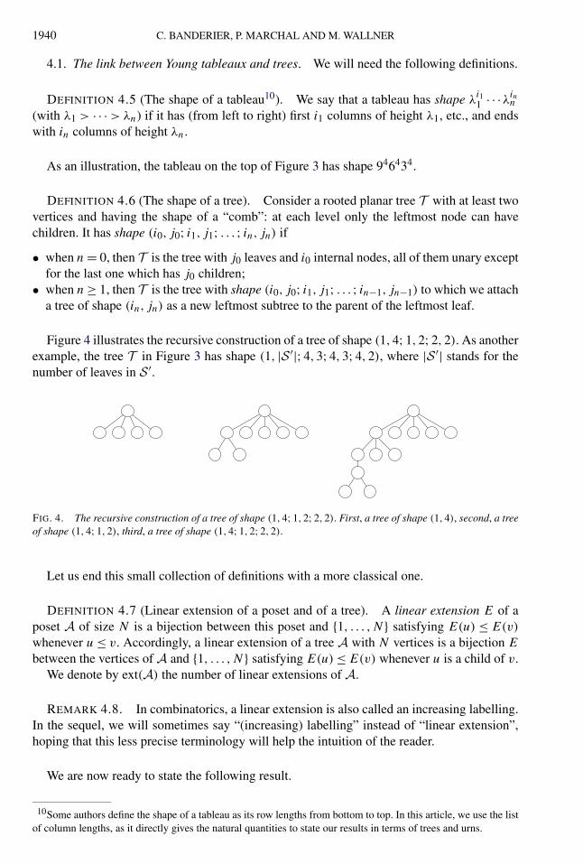
DEFINITION 4.6 (The shape of a tree). Consider a rooted planar tree T with at least twovertices and having the shape of a “comb”: at each level only the leftmost node can havechildren. It has shape (i0, j0; i1, j1; . . . ; in, jn) if
• when n = 0, then T is the tree with j0 leaves and i0 internal nodes, all of them unary exceptfor the last one which has j0 children;
• when n ≥ 1, then T is the tree with shape (i0, j0; i1, j1; . . . ; in−1, jn−1) to which we attacha tree of shape (in, jn) as a new leftmost subtree to the parent of the leftmost leaf.
Figure 4 illustrates the recursive construction of a tree of shape (1,4;1,2;2,2). As anotherexample, the tree T in Figure 3 has shape (1, |S ′|;4,3;4,3;4,2), where |S ′| stands for thenumber of leaves in S ′.
FIG. 4. The recursive construction of a tree of shape (1,4;1,2;2,2). First, a tree of shape (1,4), second, a treeof shape (1,4;1,2), third, a tree of shape (1,4;1,2;2,2).
Let us end this small collection of definitions with a more classical one.
DEFINITION 4.7 (Linear extension of a poset and of a tree). A linear extension E of aposet A of size N is a bijection between this poset and {1, . . . ,N} satisfying E(u) ≤ E(v)
whenever u ≤ v. Accordingly, a linear extension of a tree A with N vertices is a bijection E
between the vertices of A and {1, . . . ,N} satisfying E(u) ≤ E(v) whenever u is a child of v.We denote by ext(A) the number of linear extensions of A.
REMARK 4.8. In combinatorics, a linear extension is also called an increasing labelling.In the sequel, we will sometimes say “(increasing) labelling” instead of “linear extension”,hoping that this less precise terminology will help the intuition of the reader.
We are now ready to state the following result.
10Some authors define the shape of a tableau as its row lengths from bottom to top. In this article, we use the listof column lengths, as it directly gives the natural quantities to state our results in terms of trees and urns.

PÓLYA URNS AND YOUNG TABLEAUX 1941
PROPOSITION 4.9 (Link between the southeast corner of Young tableaux and linear exten-sions of trees). Fix a tableau with shape λ
i11 · · ·λin
n and consider a random uniform Youngtableau Y with this given shape. Let EY(v) be the entry of the southeast corner of this Youngtableau. Let T be a tree with shape (1,N −m−λ1 +1; i1, λ1 −λ2; i2, λ2 −λ3; . . . ; in, λn−1),where N = ∑
λkik is the size of the tableau Y and m = i1 + · · · + in is the number of itscolumns. Let ET be a random uniform linear extension of T , and vm be the mth vertex in theleftmost branch of this tree T . Then ET (vm) and 1 + EY(v) have the same law.
PROOF. The proof will be given on page 1948, as it requires two ingredients, which havetheir own interest and which are presented in the two next sections (Section 4.2 on the densitymethod for Young tableaux, and Section 4.3 on the density method for trees). �
EXAMPLE 4.10. Let us apply the previous result to the tree of shape (1,4;1,2;2,2)
from Figure 4. There we have n = 2, m = 3. Then this tree corresponds to a Young tableauof shape 5132 and size N = 11.
REMARK 4.11. In the simplest case when the tableau is a rectangle (i.e., it has shapeλ
i11 ), the associated tree has shape (1, (λ1 − 1)(i1 − 1); i1, λ1 − 1). In that case, the law of
ET (vm) is easy to compute and we get an alternative proof of the following formula, firstestablished in [63]:
P(EY(v) = k
) =(k−1i1−1
)(λ1i1−kλ1−1
)( λ1i1λ1+i1−1
) .
The fact that Y and T are related is obvious from the construction of T , but it is not a priorigranted that it will lead to a simple, nice link between the distributions of v and vm (the two
black cells in Figure 3). So, ET (vm)L= 1+EY(v) deserves a detailed proof: it will be the topic
of the next subsections. The proof has a nice feature: it uses a generic method, which we callthe density method and which was introduced in our articles [10, 64]. In fact, en passant, thesenext subsections also illustrate the efficiency of the density method in order to enumerate(and to perform uniform random generation) of combinatorial structures (like we did in thetwo aforementioned articles for permutations with some given pattern, or rectangular Youngtableaux with “local decreases”).
The advantage of Proposition 4.9 is that linear extensions of a tree are easier to studythan Young tableaux and can, in fact, be related to our periodic urn models, as shown inSection 4.3.
4.2. The density method for Young tableaux. Trees and Young tableaux can be viewedas posets [88]. We will use this point of view to prove Proposition 4.9. We recall here somegeneral facts that will be useful in the sequel.
DEFINITION 4.12 (Order polytope of a poset). Let A be a general poset with cardinalityN and order relation ≤. We can associate with A a polytope P ⊂ [0,1]A defined by thecondition (Ye)e∈A ∈ P if and only if Ye ≤ Ye′ whenever e ≤ e′. Then P is called the orderpolytope of the poset A.
EXAMPLE 4.13. Let A be the set of subsets of {a, b} ordered by inclusion. Then itsorder polytope is given by P = {(Y∅, Y{a}, Y{b}, Y{a,b}) ∈ [0,1]4 : Y∅ ≤ Y{a}, Y∅ ≤ Y{b}, Y∅ ≤Y{a,b}, Y{a} ≤ Y{a,b}, Y{b} ≤ Y{a,b}}.

1942 C. BANDERIER, P. MARCHAL AND M. WALLNER
Let Y = (Ye)e∈A ∈ [0,1]A be a tuple of random variables11 chosen according to the uni-form measure on the polytope P . Then we consider the function X having integer values,defined by Xe := k if Ye is the kth smallest real in the set of reals {Ye : e ∈ A}. It is some-times called order statistic. Note that X is a random variable, defined almost surely as wehave a zero probability that some marginals of Y have the same value, and X is uniformlydistributed on the set of all linear extensions of A. The last claim holds because the wedgesof each linear extension have equal size 1/N ! for N = |A| being the size of the poset A.
EXAMPLE 4.14. Continuing Example 4.13, there are two linear extensions of A:(X∅,X{a},X{b},X{a,b}) = (1,2,3,4) and (X∅,X{a},X{b},X{a,b}) = (1,3,2,4). They cor-respond to the following two wedges in P : Y∅ ≤ Y{a} ≤ Y{b} ≤ Y{a,b} and Y∅ ≤ Y{b} ≤ Y{a} ≤Y{a,b}. The volume of each of them is 1/24, while the volume of P is 1/12.
Conversely, if X is a random uniform increasing labelling of A, one gets a random variableY on the polytope P via Ye := TXe , where T is a random uniform N -tuple from the set{(T1, . . . , TN) ∈ [0,1]N : T1 < · · · < TN }. Therefore, Y is uniformly distributed on P . Whatis more, Tk is the kth largest uniform random variable among N independent uniform randomvariables. Thus, it has density k
(Nk
)xk−1(1 − x)N−k . As a consequence, for any e ∈ A, Ye has
density
(25) ge(x) =N∑
k=1
P(Xe = k)k
(N
k
)xk−1(1 − x)N−k.
This formula can be read as two different writings of the same polynomial in two differentbases; thus, by elementary linear algebra, it implies that P(Xe = k) can be deduced from thepolynomial ge. In particular, we have the following property.
LEMMA 4.15. Let A, A′ be two posets with the same cardinality, and let P , P ′ be theirrespective order polytopes. Let X (resp., X′) be a random linear extension of A (resp., A′).Let Y (resp., Y ′) be a uniform random variable on P (resp., P ′). Then, for any e ∈ A ande′ ∈ A′, such that Ye and Y ′
e′ have the same density, Xe and X′e′ have the same law.
Let Y be a tableau with shape λi11 . . . λ
inn and total size N = ∑
k λkik . We view Y as a poset:Y is a set of N cells equipped with a partial order “≤”, where c ≤ c′ if one can go from c
to c′ with only north and east steps. We denote by P the order polytope of the tableau Y .We will introduce an algorithm generating a random element of P according to the uniform
measure. In order to do so, we fill the diagonals one by one. Let us introduce some notation.The tableau Y can be sliced into M = λ1 + i1 +· · ·+ in −1 diagonals D1, . . . ,DM as follows:D1 is the northwest corner and recursively, Dk+1 is the set of cells which are adjacent to oneof the cells of D1 ∪ · · · ∪ Dk and which are not in D1 ∪ · · · ∪ Dk . In particular, DM is thesoutheast corner. For example, Figure 3 has M = 20 such diagonals.
Note that between two consecutive diagonals Dk and Dk+1 (let us denote their cell entriesby y1 < · · · < yj and x1 < · · · < xj ′ ), there exist four different interlocking relations illus-trated by Figure 5. The shape of the tableau implies that for each k we are in one of thesefour possibilities, each of them thus corresponds to a polytope Pk defined as:
case 1: Pk := {y1 < x1 < · · · < yj < xj },(26)
case 2: Pk := {x1 < y1 < · · · < xj < yj },(27)
case 3: Pk := {y1 < x1 < · · · < xj−1 < yj },(28)
case 4: Pk := {x1 < y1 < · · · < xj < yj < xj+1}.(29)
11When the poset is a Young tableau, this corresponds to what is called a Poissonized Young tableau in [37].

PÓLYA URNS AND YOUNG TABLEAUX 1943
FIG. 5. Young tableaux of any shape can be generated by a sequence of “diagonals,” which interlock accordingto the four possibilities above.
Our algorithm will make use of conditional densities along the M diagonals of Y . For thispurpose, for every k ∈ {1, . . . ,M} we define a polynomial gk in |Dk| variables as follows.First, one sets g1 := 1; the next polynomials are defined by induction. Suppose that 1 ≤ k ≤M − 1 and Dk = (y1 < · · · < yj). The four above-mentioned possibilities for Dk+1 lead tothe definition of the following polynomials:
1. In the first case (interlocking given by (26)), this gives
gk+1(x1, . . . , xj ) :=∫ x1
0dy1
∫ x2
x1
dy2 · · ·∫ xj
xj−1
dyjgk(y1, . . . , yj ).
2. In the second case (interlocking given by (27)), this gives
gk+1(x1, . . . , xj ) :=∫ x2
x1
dy1
∫ x3
x2
dy2 · · ·∫ xj
xj−1
dyj−1
∫ 1
xj
dyjgk(y1, . . . , yj ).
3. In the third case (interlocking given by (28)), this gives
gk+1(x1, . . . , xj−1) :=∫ x1
0dy1
∫ x2
x1
dy2 · · ·∫ 1
xj−1
dyjgk(y1, . . . , yj ).
4. In the fourth case (interlocking given by (29)), this gives
gk+1(x1, . . . , xj+1) :=∫ x2
x1
dy1
∫ x3
x2
dy2 · · ·∫ xj+1
xj
dyjgk(y1, . . . , yj ).
Now, we use these polynomials to formulate a random generation algorithm which willalso be able to enumerate the corresponding Young tableaux. Note that faster random gener-ation algorithms are known (like the hook walk from [40]), but it is striking that the abovepolynomials gk will be the key to relate the distributions of different combinatorial structures,allowing us to capture second order fluctuations in Young tableaux, trees and urns. It is alsonoteworthy that our density method is in some cases the most efficient way to enumerateand generate combinatorial objects (see [10] for applications on variants of Young tableaux,where the hook length formula is no more available, and see [23] for algorithmic subtletiesrelated to sampling conditional multivariate densities).
Recall that P is the order polytope of the tableau Y and that we want to generate a randomelement of P according to the uniform measure. The algorithm is the following. We generateby descending induction on k, for each diagonal Dk , a |Dk|-tuple of reals in [0,1] which willbe the entries of the cells of Dk .
First, remark that the functions defined by (30) and (31) in Algorithm 1 are indeed prob-ability densities. That is, they are measurable, positive functions and their integral is equalto 1. To prove this, remark first that these functions are polynomials and, therefore, measur-able. Next, by definition, as integrals of positive functions, they are positive. Finally, the factthat the integral is equal to 1 follows from their definition.

1944 C. BANDERIER, P. MARCHAL AND M. WALLNER
ALGORITHM 1 (Output: a random uniform Young tableau Y , via the density method).
Step 1. Recall that DM is the southeast corner. Generate the corresponding cell entryat random with probability density
(30)gM(x)∫ 1
0 gM(y)dy.
Step 2. By descending induction on k from M − 1 down to 1, generate the diagonal Dk
(seen as a tuple of |Dk| reals in [0,1]) according to the density
(31)gk(x1, . . . , x|Dk |)
gk+1(Dk+1)1Pk
,
where gk and 1Pkare chosen according to the cases given by (26), (27), (28), (29).
We then claim that Algorithm 1 yields a random element (D1, . . . ,DM) of P with the uni-form measure. Indeed, by construction, its density is the product of the conditional densitiesof the diagonals D1, . . . ,DM . The crucial observation now is that the product of the condi-tional densities (31) is a telescopic product, so the algorithm generates each Young tableauY with the same “probability” (or more rigorously, as we have continuous variables, with thesame density):
(32)gM(DM)∫ 1
0 gM(y)dy
M−1∏k=1
gk(Dk)
gk+1(Dk+1)1Pk
= 1{Y∈P}∫ 10 gM(y)dy
.
This indeed means that our algorithm yields a uniform random variable on the order poly-tope P . Alternatively, one can say that the Young tableau Y is a random variable on [0,1]Nwith density given by (32), therefore,∫
[0,1]N1{Z∈P} dZ =
∫ 1
0gM(y)dy.
Now, suppose that we pick uniformly at random an element Z′ of [0,1]N . Then one has
P(Z′ ∈P
) =∫[0,1]N
1{Z∈P} dZ = ext(Y)
N ! ,
where ext(Y) is the number of increasing labellings (linear extensions) of the tableau Y .Thus,
ext(Y) = N !∫ 1
0gM(y)dy.
In the next section, we turn our attention to the density method for trees.
4.3. The density method for trees. Let the tree T , its subtree S , and the verticesv0, . . . , vm be defined as on page 1939 (see Figure 3). As in Section 4.2, it is possible toconstruct a random linear extension of S by using a uniform random variable Y on the orderpolytope of S . The vertex vm has then a random value Yvm between 0 and 1, and we want tocompute its density. To this aim, we associate to each internal node vk a polynomial fk (inσk variables, where σk is the number of siblings of vk). These polynomials fk are defined byinduction starting with f1 := 1, while f2, . . . , fm−1 are defined by
fk(x0, . . . , xσk) :=
∫ inf{x0,...,xσk}
0dy0
∫ 1
0dy1 · · ·
∫ 1
0dyσk−1fk−1(y0, y1, . . . , yσk−1).

PÓLYA URNS AND YOUNG TABLEAUX 1945
The last polynomial, fm, additionally depends on the number j of children of vm:
fm(x0, . . . , xσm)
:= (1 − x0)j∫ inf{x0,...,xσm }
0dy0
∫ 1
0dy1 · · ·
∫ 1
0dyσm−1fm−1(y0, y1, . . . , yσm−1).
(33)
We also define hvm :
hvm(x) :=∫ 1
0dx1 · · ·
∫ 1
0dxσmfm(x, x1, . . . , xσm).
We claim that hvm(x) is (up to a multiplicative constant) the density of Yvm . This is shown asin Section 4.2 using Algorithm 2, which generates uniformly at random a labelling of S .
ALGORITHM 2 (Output: a random uniform increasing labelling Y of the tree S).
Step 1. Generate Yvm according to the density
hvm(x)∫ 10 hvm(x) dx
.
Step 2. If vm has j children s1, . . . , sj , then generate (Ys1, . . . , Ysj ) according to thedensity ∏j
i=1 1{yi>Yvm }(1 − Yvm)j
.
Step 3. If vm has j siblings s1, . . . , sj , then generate (Ys1, . . . , Ysj ) according to thedensity
fm(Yvm, y1, . . . , yj )∫ 10 dy1 · · · ∫ 1
0 dyjfm(Yvm, y1, . . . , yj ).
Step 4. By descending induction for k from m − 1 down to 1, if vk has j siblingss1, . . . , sj , then generate the tuple Yk = (Yvk
, Ys1, . . . , Ysj ) according to the density
fk(y0, . . . , yj )
fk+1(Yk+1)1{y0<min Yk+1}.
Indeed, the random tuple Y generated by this algorithm is by construction an element ofthe order polytope. What is more, we have the uniform distribution, as the probabilities ofall Y ’s are equal to a telescopic product similar to formula (32). Therefore, hm(x) is (up to amultiplicative constant) the density of Yvm and the number ext(S) of linear extensions of Sis given by
ext(S) = |S|!∫ 1
0hvm(x) dx.
It remains to connect the densities of v in Y and vm in S ; we do this in the followinglemma.

1946 C. BANDERIER, P. MARCHAL AND M. WALLNER
LEMMA 4.16. The polynomial gM(x) (which gives the density of v, the southeast cornerof the Young tableau Y) and the polynomial hvm(x) (which gives the density of vm in thetree S) are equal up to a multiplicative constant:
hvm(x) = cgM(x) with c = |Y|!|S|!
ext(S)
ext(Y).
PROOF. The main idea of the proof consists in adding a filament to the tree and to thetableau, and inspecting the consequences via the density method.
Part 1 (adding a filament to the tableau). Let YL be the tableau obtained by adding toY L cells horizontally to the right of its southeast corner v (and denote these new cells bye1, . . . , eL). We can generate a random element of the order polytope of YL as follows: remarkthat Y is a subtableau of YL and that the first M diagonals D1, . . . ,DM of YL are the same asthe first M diagonals of Y (recall that the diagonals are lines with positive slope +1, startingfrom each cell of the first column and row). In particular, DM is the southeast corner cell v.Then we can extend Algorithm 1 in the following way:
ALGORITHM 3 (Output: a random uniform increasing labelling X of the tableau with L
added cells).
Step 1. Generate XM,L the entry of the cell v according to the density
gM,L(x)∫ 10 gM,L(y) dy
where gM,L(x) := gM(x)(1 − x)L
L! .
Step 2. Generate the entries of the diagonals DM−1, . . . ,D1 as in Algorithm 1.Step 3. Generate the entry X1 of e1 with density
L(1 − x)L−1
(1 − XM,L)L1{x>XM,L}.
Step 4. For i from 1 to L − 1, generate the entry Xi+1 of ei+1 with density
(L − i)(1 − x)L−i−1
(1 − Xi)L−i1{x>Xi}.
Using the same arguments as for Algorithm 1, we can show that Algorithm 3 yields auniform random variable on the order polytope of YL and that the number of increasinglabellings of YL is
ext(YL) = (N + L)!∫ 1
0gM,L(y) dy = (N + L)!
∫ 1
0
gM(y)(1 − y)L
L! dy.
On the other hand, using the hook length formula, we see that the hook lengths of YL arethe same as those of Y , except for the first row. A straightforward computation shows that
ext(Y)
N ! = ext(YL)
(N + L)! × GL,
where, as Y has shape λi11 · · ·λin
n , the constant GL is given by
(34) GL = L!n∏
k=1
(i1 + · · · + ik + L + λk − 1)ik
(i1 + · · · + ik + λk − 1)ik,

PÓLYA URNS AND YOUNG TABLEAUX 1947
where we reuse the falling factorial notation ab = a(a − 1) · · · (a − b + 1). This leads to
(35)∫ 1
0gM(y)(1 − y)L dy = L!
GL
ext(Y)
N ! .
Part 2 (adding a filament to the tree). Suppose that we extend the tree S by adding a fila-ment of length L. Let SL be the tree obtained from S by attaching to vm a subtree consistingof a line with L vertices. Put
fL(x) := (1 − x)Lhvm(x)
L! .
With the same arguments as for the function hvm defined in (33), we see that fL/∫ 1
0 fL(x) dx
is the density of YL(vm) where YL is a uniform random variable on the order polytope of SL.Following the same reasoning, we can show that the number of linear extensions of SL is
ext(SL) = (|S| + L)!∫ 1
0fL(y) dy.
On the other hand, recall that a version of the hook length formula holds for trees (see, e.g.,[41, 55, 82]): the number of linear extensions of a tree of size N is given by
N !∏v∈S hook(v)
,
where here hook(v) is the number of descendants of v (including v itself).Applying this formula to the tree S yields
ext(S)
|S|! = ext(SL)
(|S| + L)! × GL,
with the same GL as in (34). Indeed, the most crucial point is that the hook lengths of theYoung tableau on the first row are the same as the hook lengths of the tree along the leftmostbranch. This key construction allows us to connect these two structures. Hence, one has
(36)∫ 1
0hvm(y)(1 − y)L dy = L!
GL
ext(S)
|S|! .
Part 3 (linking tableaux and trees). Comparing (35) and (36), we get for any integer L ≥ 1,∫ 1
0hvm(y)(1 − y)L dy = c
∫ 1
0gM(y)(1 − y)L dy,
where c is the constant given by
c = |Y|!|S|!
ext(S)
ext(Y).
Since hvm(x) and gM(x) are polynomials, this implies that hvm = cgM . �
Before establishing the final link between Young tableaux and urns, we start by collectingwhat we got via the density method: this gives the proof of Proposition 4.9, which we nowrestate.
PROPOSITION 4.9 (Link between the corner of a Young tableau and linear extensions oftrees). Fix a tableau with shape λ
i11 · · ·λin
n and consider a random uniform Young tableau Ywith this given shape. Let EY(v) be the entry of the southeast corner of this Young tableau.Let T be a tree with shape (1,N −m−λ1 +1; i1, λ1 −λ2; i2, λ2 −λ3; . . . ; in, λn −1), whereN = ∑
λkik is the size of the tableau Y and m = i1 + · · · + in is the number of its columns.Let ET be a random uniform linear extension of T , and vm be the mth vertex in the leftmostbranch of this tree T . Then ET (vm) and 1 + EY(v) have the same law.

1948 C. BANDERIER, P. MARCHAL AND M. WALLNER
PROOF. The reader is invited to have a new look on Figure 3 (page 1938), which illus-trates for this proof the idea of the trees T , S and the set of leaves S ′. We first introduce aforest T ∗ := S ∪ S ′ obtained by adding N − m − λ1 + 1 vertices without any order relationto the tree S . T ∗ has an order relation inherited from the order relation ≤ on S : two nodes x,y of T ∗ are comparable if and only if they belong to S and in that case, the order relation onT ∗ is the same as the one on S .
Let P ′ be the order polytope of S . Then it is clear that the order polytope of T ∗ is
P = P ′ × [0,1]N−m−λ1+1.
In particular, if Y ′ is a uniform random variable on P ′ and if Y is a uniform random variableon P , then Y ′
v and Yv have the same density. This density is proportional to the function hvm
computed in Section 4.3. Next, recall the notation gM and DM from Section 4.2. Lemma 4.16gives that hvm = cgM . Thus, the density of Yvm is the same as the density of DM . Moreover,T ∗ and Y have the same cardinality. Therefore, Lemma 4.15 entails that if ET ∗ is a randomuniform linear extension of T ∗ and if EY(v) is the entry of the southeast corner in a randomincreasing labelling of Y , then ET ∗(vm) and EY(v) have the same distribution.
Now, it is easy to deduce from ET ∗ a random uniform linear extension ET of T : setET (u) = 1 if u is the root of T , and set ET (u) = 1 + ET ∗(u) for the other nodes (since anysuch node u can be identified as a node of T ). Applying this to the vertex vm completes theproof of Proposition 4.9. �
4.4. The link between trees and urns. In order to end the proof of Theorem 4.2, we needtwo more propositions.
PROPOSITION 4.17 (Link between trees and urns). Consider a tree S with shape(i1, j1; . . . ; in, jn). Let v be the parent of the leftmost leaf if jn ≥ 1, or the leftmost leaf ifjn = 0. Let ES be a random uniform linear extension of S .
Let X = |S|−ES(v). Then X has the same law as the number of black balls in the follow-ing urn process:
• Initialize the urn with b0 := jn + 1 black balls and w0 := in white balls.• For k from n − 1 to 1, perform the following steps:
1. Perform jk − 1 times the classical Pólya urn with replacement matrix( 1 0
0 1
).
2. Make one transition with the replacement matrix( 1 ik
0 1+ik
).
REMARK 4.18. Note that the urn scheme described in the proposition is precisely themodel of periodic Pólya urns covered by Theorem 3.8. For Young–Pólya urns, one has ik = �
and jk = p for k < n, and in = � and jn = p − 1, compare Figure 3.
PROOF OF PROPOSITION 4.17. First, consider the transition probabilities in the classicalPólya urn. At step i > 0, the composition (Bi,Wi) is obtained from (Bi−1,Wi−1) by addinga black ball with probability Bi−1
Bi−1+Wi−1and a white ball with probability Wi−1
Bi−1+Wi−1. We will
now show that the same transition probabilities are imposed by the linear extension of thetree.
We start with a definition. If R ⊂ S we define ER : R → {1, . . . , |R|} as the only bijectionpreserving the order relation induced by ES . That is, ER(u) = k if and only if ES(u) is thekth smallest value in the set {ES(r) : r ∈ R}. It is easy to check that ER is a uniform linearextension of R seen as a poset equipped with the order relation inherited from S .
Let us prove our claim. On the one hand, for every vertex w which is one of the jn childrenof v, we have ES(w) > ES(v). On the other hand, for every vertex u which is one of the in−1
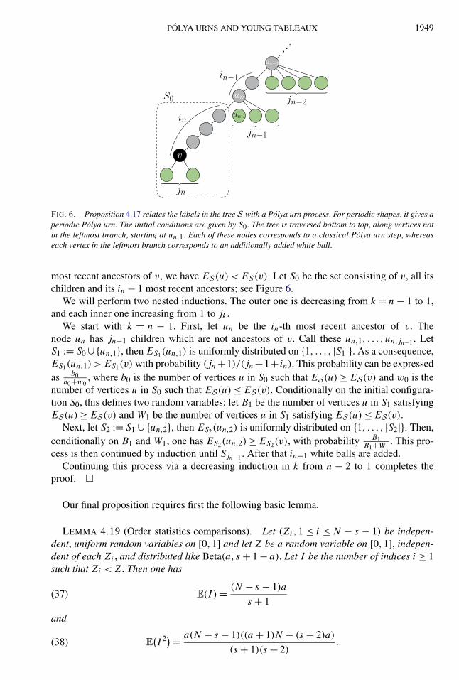
PÓLYA URNS AND YOUNG TABLEAUX 1949
FIG. 6. Proposition 4.17 relates the labels in the tree S with a Pólya urn process. For periodic shapes, it gives aperiodic Pólya urn. The initial conditions are given by S0. The tree is traversed bottom to top, along vertices notin the leftmost branch, starting at un,1. Each of these nodes corresponds to a classical Pólya urn step, whereaseach vertex in the leftmost branch corresponds to an additionally added white ball.
most recent ancestors of v, we have ES(u) < ES(v). Let S0 be the set consisting of v, all itschildren and its in − 1 most recent ancestors; see Figure 6.
We will perform two nested inductions. The outer one is decreasing from k = n − 1 to 1,and each inner one increasing from 1 to jk .
We start with k = n − 1. First, let un be the in-th most recent ancestor of v. Thenode un has jn−1 children which are not ancestors of v. Call these un,1, . . . , un,jn−1 . LetS1 := S0 ∪{un,1}, then ES1(un,1) is uniformly distributed on {1, . . . , |S1|}. As a consequence,ES1(un,1) > ES1(v) with probability (jn +1)/(jn +1+ in). This probability can be expressedas b0
b0+w0, where b0 is the number of vertices u in S0 such that ES(u) ≥ ES(v) and w0 is the
number of vertices u in S0 such that ES(u) ≤ ES(v). Conditionally on the initial configura-tion S0, this defines two random variables: let B1 be the number of vertices u in S1 satisfyingES(u) ≥ ES(v) and W1 be the number of vertices u in S1 satisfying ES(u) ≤ ES(v).
Next, let S2 := S1 ∪ {un,2}, then ES2(un,2) is uniformly distributed on {1, . . . , |S2|}. Then,conditionally on B1 and W1, one has ES2(un,2) ≥ ES2(v), with probability B1
B1+W1. This pro-
cess is then continued by induction until Sjn−1 . After that in−1 white balls are added.Continuing this process via a decreasing induction in k from n − 2 to 1 completes the
proof. �
Our final proposition requires first the following basic lemma.
LEMMA 4.19 (Order statistics comparisons). Let (Zi,1 ≤ i ≤ N − s − 1) be indepen-dent, uniform random variables on [0,1] and let Z be a random variable on [0,1], indepen-dent of each Zi , and distributed like Beta(a, s + 1 − a). Let I be the number of indices i ≥ 1such that Zi < Z. Then one has
(37) E(I ) = (N − s − 1)a
s + 1
and
(38) E(I 2) = a(N − s − 1)((a + 1)N − (s + 2)a)
(s + 1)(s + 2).
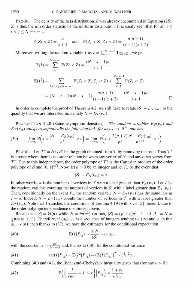
1950 C. BANDERIER, P. MARCHAL AND M. WALLNER
PROOF. The density of the beta distribution Z was already encountered in Equation (25);Z is thus the ath order statistic of the uniform distribution. It is easily seen that for all 1 ≤i < j ≤ N − s − 1,
P(Zi < Z) = a
s + 1and P(Zi < Z,Zj < Z) = a(a + 1)
(s + 1)(s + 2).
Moreover, writing the random variable I as I = ∑N−s−1i=1 1{Zi<Z}, we get
E(I ) =N−s−1∑
i=1
P(Zi < Z) = (N − s − 1)a
s + 1,
E(I 2) = ∑
1≤i �=j≤N−s−1
P(Zi < Z,Zj < Z) +N−s−1∑
i=1
P(Zi < Z)
= (N − s − 1)(N − s − 2)a(a + 1)
(s + 1)(s + 2)+ (N − s − 1)a
s + 1. �
In order to complete the proof of Theorem 4.2, we still have to relate |S| − ES(vm) to thequantity that we are interested in, namely N − ET (vm).
PROPOSITION 4.20 (Same asymptotic densities). The random variables ES(vm) andET (vm) satisfy asymptotically the following link: for any s, t ∈ R
+, one has
(39) limn→∞P
(s <
|S| − ES(vm)
nδ< t
)= lim
n→∞P
(s <
2(p + �)
p�
N − ET (vm)
n1+δ< t
).
PROOF. Let T ∗ = S ∪ S ′ be the graph obtained from T by removing the root. Then T ∗is a poset where there is no order relation between any vertex of S ′ and any other vertex fromT ∗. Due to this independence, the order polytope of T ∗ is the Cartesian product of the orderpolytope of S and [0,1]|S ′|. Now, let a > 0 be an integer and let Fa be the event that
|S| − ES(vm) = a.
In other words, a is the number of vertices in S with a label greater than ES(vm). Let I bethe random variable counting the number of vertices in S ′ with a label greater than ET (vm).Then, conditionally on the event Fa , the random variable N − ET (vm) has the same law asI + a. Indeed, N − ET (vm) counts the number of vertices in T with a label greater thanET (vm). Note that I satisfies the conditions of Lemma 4.19 (with s := |S| therein), due tothe order polytope independence mentioned above.
Recall that |S| = �(n) while N = �(n2) (in fact, |S| = (p + �)n − 1 and |T | = N =12p�n(n + 1)). Therefore, if (an)n≥1 is a sequence of integers tending to +∞ and such thatan = o(n), then thanks to (37), we have the estimates for the conditional expectation
(40) E(I |Fan) ∼ anN
|S| ∼ cnan,
with the constant c = p�2(p+�)
and, thanks to (38), for the conditional variance
(41) var(I |Fan) = E(I 2|Fan
) − (E(I |Fan)
)2 ∼ c2n2an.
Combining (40) and (41), the Bienaymé–Chebyshev inequality gives that (for any κ > 0):
(42) P
({∣∣∣∣ I
cnan
− 1∣∣∣∣ > κ
}∣∣∣Fan
)≤ 1 + εn
κ2an
,

PÓLYA URNS AND YOUNG TABLEAUX 1951
where εn is a sequence converging to 0 as n → ∞. Since we have
N − ET (vm)
nan
= I + an
nan
= I
nan
+ 1
n,
the inequality (42) can be rewritten into
(43) P
({∣∣∣∣N − ET (vm)
cnan
− 1∣∣∣∣ > κ
}∣∣∣Fan
)≤ 1 + ε′
n
κ2an
,
where ε′n is a sequence converging to 0 as n → ∞. In particular, for any t > 0 and 0 < δ < 1,
setting an = �tnδ� in (43) gives
(44) P
({∣∣∣∣N − ET (vm)
cn1+δ− t
∣∣∣∣ > κt
}∣∣∣Fan
)≤ 1 + o(1)
κ2tnδ.
Finally, for all reals 0 < s < t , define the event
Fs,t = ⋃snδ<a<tnδ
Fa ={s <
|S| − ES(vm)
nδ< t
}.
According to (44) (set κ = ε/t for any ε > 0), we have for n → ∞
P
({s <
N − ET (vm)
cn1+δ< t
}∣∣∣Fs,t
)→ 1.
Thus, conditioning on the complementary event Fs,t , we have
(45) limn→∞P
({s <
N − ET (vm)
cn1+δ< t
}∩ Fs,t
)= 0,
whereas conditioning on Fs,t gives
(46) limn→∞P
({s <
N − ET (vm)
cn1+δ< t
}∩ Fs,t
)= lim
n→∞P
(s <
|S| − ES(vm)
nδ< t
).
Summing (45) and (46) leads to (39). �
In summary, in this section we have proven that the four following quantities have asymp-totically the same distribution:
(47)
2
p�
N − EY(v)
n1+δ= 2
p�
N − ET (vm)
n1+δProp. 4.9 (density method)
∼ 1
p + �
|S| − ES(vm)
nδProp. 4.20 (order statistics)
= 1
p + �
B(n−1)p
nδ. Prop. 4.17 (Pólya urn)
In conjunction with Theorem 1.6 proven via analytic combinatorics methods, this implies thatthe four quantities in (47) converge in law to the distribution GenGammaProd(p, �, b0,w0),when δ = p/(p + �). This is exactly the statement of Theorem 4.2.
NOTA BENE. It should be stressed that the sequence of transformations in (47) is not abijection between Young tableaux and urns, it is only asymptotically that the correspondingdistributions are equal.
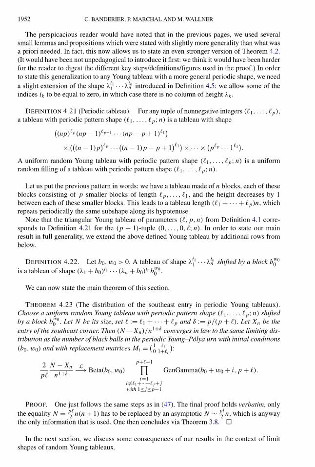
1952 C. BANDERIER, P. MARCHAL AND M. WALLNER
The perspicacious reader would have noted that in the previous pages, we used severalsmall lemmas and propositions which were stated with slightly more generality than what wasa priori needed. In fact, this now allows us to state an even stronger version of Theorem 4.2.(It would have been not unpedagogical to introduce it first: we think it would have been harderfor the reader to digest the different key steps/definitions/figures used in the proof.) In orderto state this generalization to any Young tableau with a more general periodic shape, we needa slight extension of the shape λ
i11 · · ·λin
n introduced in Definition 4.5: we allow some of theindices ik to be equal to zero, in which case there is no column of height λk .
DEFINITION 4.21 (Periodic tableau). For any tuple of nonnegative integers (�1, . . . , �p),a tableau with periodic pattern shape (�1, . . . , �p;n) is a tableau with shape(
(np)�p(np − 1)�p−1 · · · (np − p + 1)�1)
× (((n − 1)p
)�p · · · ((n − 1)p − p + 1)�1
) × · · · × (p�p · · ·1�1
).
A uniform random Young tableau with periodic pattern shape (�1, . . . , �p;n) is a uniformrandom filling of a tableau with periodic pattern shape (�1, . . . , �p;n).
Let us put the previous pattern in words: we have a tableau made of n blocks, each of theseblocks consisting of p smaller blocks of length �p, . . . , �1, and the height decreases by 1between each of these smaller blocks. This leads to a tableau length (�1 + · · · + �p)n, whichrepeats periodically the same subshape along its hypotenuse.
Note that the triangular Young tableau of parameters (�,p,n) from Definition 4.1 corre-sponds to Definition 4.21 for the (p + 1)-tuple (0, . . . ,0, �;n). In order to state our mainresult in full generality, we extend the above defined Young tableau by additional rows frombelow.
DEFINITION 4.22. Let b0,w0 > 0. A tableau of shape λi11 · · ·λin
n shifted by a block bw00
is a tableau of shape (λ1 + b0)i1 · · · (λn + b0)
inbw00 .
We can now state the main theorem of this section.
THEOREM 4.23 (The distribution of the southeast entry in periodic Young tableaux).Choose a uniform random Young tableau with periodic pattern shape (�1, . . . , �p;n) shiftedby a block b
w00 . Let N be its size, set � := �1 + · · · + �p and δ := p/(p + �). Let Xn be the
entry of the southeast corner. Then (N −Xn)/n1+δ converges in law to the same limiting dis-tribution as the number of black balls in the periodic Young–Pólya urn with initial conditions(b0,w0) and with replacement matrices Mi = ( 1 �i
0 1+�i
):
2
p�
N − Xn
n1+δ
L−→ Beta(b0,w0)
p+�−1∏i=1
i �=�1+···+�j+j
with 1≤j≤p−1
GenGamma(b0 + w0 + i, p + �).
PROOF. One just follows the same steps as in (47). The final proof holds verbatim, onlythe equality N = p�
2 n(n + 1) has to be replaced by an asymptotic N ∼ pl2 n, which is anyway
the only information that is used. One then concludes via Theorem 3.8. �
In the next section, we discuss some consequences of our results in the context of limitshapes of random Young tableaux.
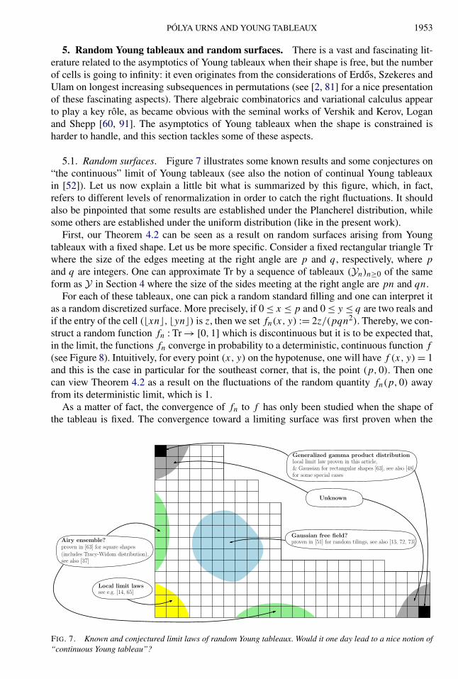
PÓLYA URNS AND YOUNG TABLEAUX 1953
5. Random Young tableaux and random surfaces. There is a vast and fascinating lit-erature related to the asymptotics of Young tableaux when their shape is free, but the numberof cells is going to infinity: it even originates from the considerations of Erdos, Szekeres andUlam on longest increasing subsequences in permutations (see [2, 81] for a nice presentationof these fascinating aspects). There algebraic combinatorics and variational calculus appearto play a key rôle, as became obvious with the seminal works of Vershik and Kerov, Loganand Shepp [60, 91]. The asymptotics of Young tableaux when the shape is constrained isharder to handle, and this section tackles some of these aspects.
5.1. Random surfaces. Figure 7 illustrates some known results and some conjectures on“the continuous” limit of Young tableaux (see also the notion of continual Young tableauxin [52]). Let us now explain a little bit what is summarized by this figure, which, in fact,refers to different levels of renormalization in order to catch the right fluctuations. It shouldalso be pinpointed that some results are established under the Plancherel distribution, whilesome others are established under the uniform distribution (like in the present work).
First, our Theorem 4.2 can be seen as a result on random surfaces arising from Youngtableaux with a fixed shape. Let us be more specific. Consider a fixed rectangular triangle Trwhere the size of the edges meeting at the right angle are p and q , respectively, where p
and q are integers. One can approximate Tr by a sequence of tableaux (Yn)n≥0 of the sameform as Y in Section 4 where the size of the sides meeting at the right angle are pn and qn.
For each of these tableaux, one can pick a random standard filling and one can interpret itas a random discretized surface. More precisely, if 0 ≤ x ≤ p and 0 ≤ y ≤ q are two reals andif the entry of the cell (�xn�, �yn�) is z, then we set fn(x, y) := 2z/(pqn2). Thereby, we con-struct a random function fn : Tr → [0,1] which is discontinuous but it is to be expected that,in the limit, the functions fn converge in probability to a deterministic, continuous function f
(see Figure 8). Intuitively, for every point (x, y) on the hypotenuse, one will have f (x, y) = 1and this is the case in particular for the southeast corner, that is, the point (p,0). Then onecan view Theorem 4.2 as a result on the fluctuations of the random quantity fn(p,0) awayfrom its deterministic limit, which is 1.
As a matter of fact, the convergence of fn to f has only been studied when the shape ofthe tableau is fixed. The convergence toward a limiting surface was first proven when the
FIG. 7. Known and conjectured limit laws of random Young tableaux. Would it one day lead to a nice notion of“continuous Young tableau”?

1954 C. BANDERIER, P. MARCHAL AND M. WALLNER
FIG. 8. Random generation of Young tableaux, seen as random surfaces (the colours correspond to level lines):• top: triangular Young tableaux (size 60 × 60, seen as histogram, and 200 × 200),• bottom: rectangular and triangular Young tableaux (400 × 200 and 410 × 20).
If one watches such surfaces from above, then one sees exactly the triangular/rectangular shapes, but one loses the3D effect. The images are generated via our own Maple package available at https:// lipn.fr/~cb/YoungTableaux,relying on a variant of the hook-length walk of [40].
limit shape is a finite union of rectangles; see Biane [13]. There the limiting surface can beinterpreted in terms of characters of the symmetric group and free probability but this leadsto complicated computations from which it is difficult to extract explicit expressions.
For rectangular Young tableaux, the limiting surface is described more precisely by Pitteland Romik [73]. A limiting surface also exists for staircase tableaux: it can be obtained by tak-ing the limiting surface of a square tableau and cutting it along the diagonal; see [4, 59]. Thisidea does not work for rectangular (nonsquare) Young tableaux: if one cuts such tableauxalong the diagonal, one does not get the limiting surface of triangular Young tableaux (thehypotenuse would have been the level line 1, but the diagonal is in fact not even a level line,as visible in Figure 8 and proven in [73]).
Apart from the particular cases mentioned above, convergence results for surfaces arisingfrom Young tableau seem to be lacking. There are also very few results about the fluctuationsaway from the limiting surface. For rectangular shapes, these fluctuations were studied byMarchal [63]: they are Gaussian in the southeast and northwest corner, while the fluctuationson each edge follow a Tracy–Widom limit law, at least when the rectangle is a square (forgeneral rectangles, there remain some technicalities, although the expected behaviour is thesame). For staircase triangles, Gorin and Rahman [37] use a sorting network representationto obtain asymptotic formulas using double integrals. In particular, they find the limit law onthe edge. Their approach may be generalizable to other triangular shapes. Also, instead ofrenormalized limits, one may be interested in local limits, there are then nice links with thefamous jeu de taquin [86] and characters of symmetric groups [14].
There is another framework where random surfaces naturally arise, namely random tilingsand related structures (see, e.g., [85]). Indeed, one can associate a height function with a

PÓLYA URNS AND YOUNG TABLEAUX 1955
tiling: this gives an interpretation as a surface. In this framework, there are results on thefluctuations of these surfaces, which are similar to the ones on Young tableaux. In the caseof the Aztec diamond shape, Johansson and Nordenstam [48] proved that the fluctuations ofthe Artic curve are related to eigenvalues of GUE minors (and are therefore Gaussian nearthe places where the curve is touching the edges, whereas they are Tracy–Widomian whenthe curve is far away from the edges). Note that this gives the same limit laws as for theArtic curve of a TASEP jump process associated to rectangular Young tableaux [63, 80].Similar results were also obtained for pyramid partitions [17, 18]. Moreover, in other modelsof lozenge tilings, it is proven that for some singular points, other limit laws appear: they arecalled cusp-Airy distributions, and are related to the Airy kernel [25]. It has to be noticedthat, up to our knowledge, the generalized gamma distributions, which appear in our results,have not been found in the framework of random tilings.
A major challenge would be to capture the fluctuations of the surface in the interior of thedomain. For Young tableaux, it is reasonable to conjecture that these fluctuations could besimilar to those observed for random tilings: in this framework, Kenyon [51] and Petrov [72]proved that the fluctuations are given by the Gaussian free field (see also [20]).
Finally, a dual question would be: in which cell does a given entry lie in a random fillingof the tableau? In the case of triangular shapes like ours, if we look at the largest entry, weget the following.
PROPOSITION 5.1 (Limit law for the location of the maximum in a triangular Youngtableau). Choose a uniform random triangular Young tableau of parameters (�,p,n) (seeDefinition 4.1). Let Posin ∈ {1, . . . , �n} be the x-coordinate of the cell containing the largestentry. Then one has
Posin�n
L−→ Arcsine(δ) where δ := p/(p + �).
PROOF. Remove from the Young tableau Y the cell containing its largest entry, andcall Y∗ this new tableau. Then, using the hook length formula, the probability that the largestentry of Y is situated at x-coordinate k� is
P(Posin = k�) =∏
c∈Y∗ hookY∗(c)∏c∈Y hookY(c)
= ∏c∈Y∗with (x-coord of c) = k�
or (y-coord of c) = (n − k + 1)p
hookY∗(c)
1 + hookY∗(c).
An easy computation then gives (with δ = p/(p + �)):
P(Posin = k�) ∼ (k/n)δ−1(1 − k/n)−δ
�(δ)�(1 − δ)
1
n.
Here, one recognizes an instance of the generalized arcsine law on [0,1] with density
xδ−1(1 − x)−δ
�(δ)�(1 − δ). �
So, if we compare models with different p and �, then the largest entry will have thetendency to be on the top of the hypotenuse when � is much larger than p, while it will beon its bottom if p is much larger than � (and on the bottom or the top with equally highprobabilities when p ≈ �); see Figure 8. This is in sharp contrast with the case of an n ×n square tableau where, for t ∈ (0,1), the cell containing the entry tn2 is asymptoticallydistributed according to the Wigner semicircle law on its level line; see [73]. We also referto Romik [79] for further discussions on Young tableau landscapes and to Morales, Pak andPanova [66] for recent results on skew-shaped tableaux.
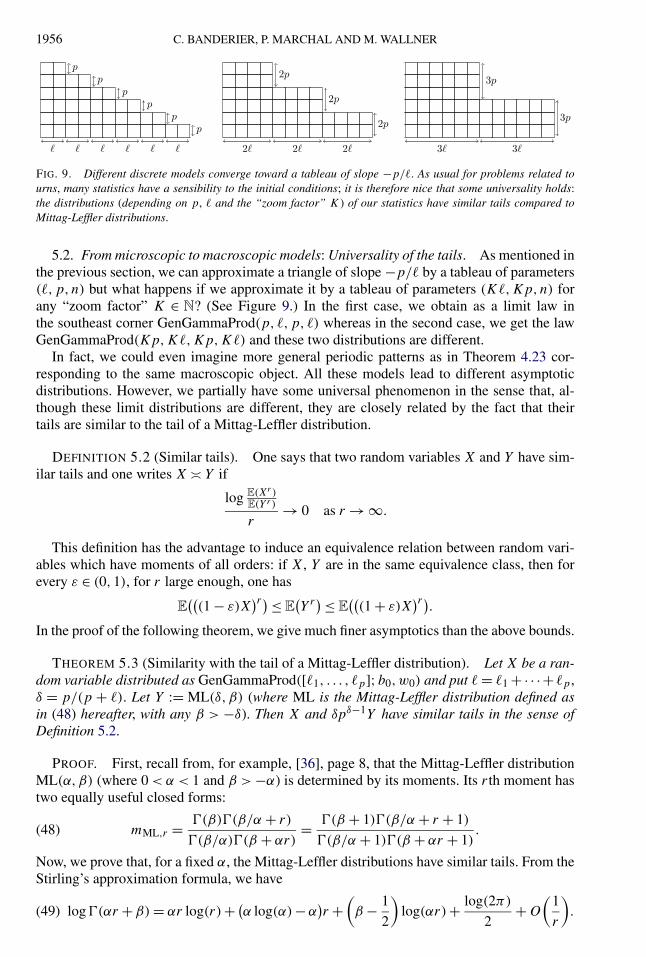
1956 C. BANDERIER, P. MARCHAL AND M. WALLNER
FIG. 9. Different discrete models converge toward a tableau of slope −p/�. As usual for problems related tourns, many statistics have a sensibility to the initial conditions; it is therefore nice that some universality holds:the distributions (depending on p, � and the “zoom factor” K) of our statistics have similar tails compared toMittag-Leffler distributions.
5.2. From microscopic to macroscopic models: Universality of the tails. As mentioned inthe previous section, we can approximate a triangle of slope −p/� by a tableau of parameters(�,p,n) but what happens if we approximate it by a tableau of parameters (K�,Kp,n) forany “zoom factor” K ∈ N? (See Figure 9.) In the first case, we obtain as a limit law inthe southeast corner GenGammaProd(p, �,p, �) whereas in the second case, we get the lawGenGammaProd(Kp,K�,Kp,K�) and these two distributions are different.
In fact, we could even imagine more general periodic patterns as in Theorem 4.23 cor-responding to the same macroscopic object. All these models lead to different asymptoticdistributions. However, we partially have some universal phenomenon in the sense that, al-though these limit distributions are different, they are closely related by the fact that theirtails are similar to the tail of a Mittag-Leffler distribution.
DEFINITION 5.2 (Similar tails). One says that two random variables X and Y have sim-ilar tails and one writes X � Y if
log E(Xr)E(Y r )
r→ 0 as r → ∞.
This definition has the advantage to induce an equivalence relation between random vari-ables which have moments of all orders: if X, Y are in the same equivalence class, then forevery ε ∈ (0,1), for r large enough, one has
E((
(1 − ε)X)r) ≤ E
(Y r) ≤ E
(((1 + ε)X
)r).
In the proof of the following theorem, we give much finer asymptotics than the above bounds.
THEOREM 5.3 (Similarity with the tail of a Mittag-Leffler distribution). Let X be a ran-dom variable distributed as GenGammaProd([�1, . . . , �p];b0,w0) and put � = �1 +· · ·+ �p ,δ = p/(p + �). Let Y := ML(δ, β) (where ML is the Mittag-Leffler distribution defined asin (48) hereafter, with any β > −δ). Then X and δpδ−1Y have similar tails in the sense ofDefinition 5.2.
PROOF. First, recall from, for example, [36], page 8, that the Mittag-Leffler distributionML(α,β) (where 0 < α < 1 and β > −α) is determined by its moments. Its r th moment hastwo equally useful closed forms:
mML,r = �(β)�(β/α + r)
�(β/α)�(β + αr)= �(β + 1)�(β/α + r + 1)
�(β/α + 1)�(β + αr + 1).(48)
Now, we prove that, for a fixed α, the Mittag-Leffler distributions have similar tails. From theStirling’s approximation formula, we have
(49) log�(αr +β) = αr log(r)+ (α log(α)−α
)r +
(β − 1
2
)log(αr)+ log(2π)
2+O
(1
r
).

PÓLYA URNS AND YOUNG TABLEAUX 1957
Applying this to the moments (48) of the Mittag-Leffler distribution Y = ML(α,β), we get
logE(Y r) = (1 − α)r log(r) + (−α log(α) + α − 1
)r +
(β
α− β
)log(r) + O(1),(50)
and thus if one compares with another distribution Y ′ = ML(α,β ′), this leads to Y � Y ′.Next, we prove that GenGammaProd distributions with the same δ have similar tails. The
moments of X = GenGammaProd([�1, . . . , �p];b0,w0) are given by formula (21). Using theapproximation (49), we get
logE(Xr) = (1 − δ)r log(r) + (1 − δ)
(log
(δ
p
)− 1
)r
+(b0 + s0δ + (1 + δ)(p − 1)
2− δ
p
p−1∑j=0
j∑k=1
�k
)log(r) + O(1).
(51)
Here, we see that in fact up to order O(r) only the slope δ and the period length p play arôle; it is only at order o(r) that b0, s0, and the �k really occur. Thus, if we now also considerX′ = GenGammaProd([�′
1, . . . , �′p′ ];b′
0,w′0), we directly deduce X � (
pp′ )δ−1X′.
Finally, we can compare the moments of X (any GenGammaProd distribution associated toa slope δ and period p) and Y (any Mittag-Leffler distribution with α := δ) via formulas (50)and (51), this leads to X � δpδ−1Y . �
REMARK 5.4. The tails of this distribution are universal: they depend only on the slopeδ and the period length p. They depend neither on the initial conditions b0 and w0, nor onfurther details of the geometry of the periodic pattern (the �i ’s).
One more universal property which holds for some families of urn distributions is that theypossess sub-Gaussian tails, a notion introduced by Kahane in [49] (see also [56] for some urnmodels exhibiting this behaviour).
DEFINITION 5.5. A random variable X has sub-Gaussian tails if there exist two con-stants c,C > 0, such that
P(|X| ≥ t
) ≤ Ce−ct2, t > 0.
PROPOSITION 5.6. The GenGammaProd(p, �, b0,w0) distributions have subGaussiantails if and only if p ≥ �.
PROOF. The GenGammaProd distribution, as defined in equation (1), has moments givenin equation (20). As derived thereafter, it has moments asymptotically equivalent to
(mr)1/r = (
(p + �)e)(δ−1)
r(1−δ)(1 + o(1)).
By [49], Proposition 9, a random variable X has sub-Gaussian tails if and only if there existsa constant K > 0 such that for all r > 0 we have (E(Xr))1/r ≤ K
√r . As δ = p
p+�the claim
follows. �
Another useful notion which helps to gain insight into the limit of Young tableaux is thenotion of a level line: let Cv be the curve separating the cells with an entry bigger than v andthe cells with an entry smaller than v (and to get a continuous curve, one follows the borderof the Young tableau if needed; see Figure 10).
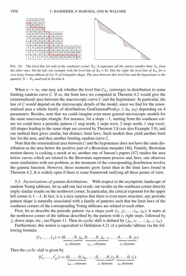
1958 C. BANDERIER, P. MARCHAL AND M. WALLNER
FIG. 10. The level line (in red) of the southeast corner Xn: it separates all the entries smaller than Xn fromthe other ones. On the left: one example with the level line of Xn = 42. One the right: the level line of Xn, for avery large Young tableau of size N of triangular shape. The area between this level line and the hypotenuse is thequantity N − Xn analysed in Section 4.
When n → ∞, one may ask whether the level line CXn converges in distribution to somelimiting random curve C. If so, the limit laws we computed in Theorem 4.2 would give the(renormalized) area between the macroscopic curve C and the hypotenuse. In particular, thelaw of C would depend on the microscopic details of the model, since we find for the renor-malized area a whole family of distributions GenGammaProd(p, �, b0,w0) depending on 4parameters. Besides, note that we could imagine even more general microscopic models forthe same macroscopic triangle. For instance, for a slope −1, starting from the southeast cor-ner we could have a periodic pattern (1 step north, 2 steps west, 2 steps north, 1 step west).All shapes leading to the same slope are covered by Theorem 3.8 (see also Example 3.9), andour method then gives similar, but distinct, limit laws. Such models thus yield another limitlaw for the area, and thus another limiting random curve C.
Note that the renormalized area between C and the hypotenuse does not have the same dis-tribution as the area below the positive part of a Brownian meander [46]. Funnily, Brownianmotion theory is cocking a snook at us: another one of Janson’s papers [47] studies the areabelow curves which are related to the Brownian supremum process and, here, one observesmore similarities with our problem, as the moments of the corresponding distribution involvethe gamma function. However, these moments grow faster than in the limit laws found inTheorem 4.2. It is widely open if there is some framework unifying all these points of view.
5.3. Factorizations of gamma distributions. With respect to the asymptotic landscape ofrandom Young tableaux, let us add one last result: our results on the southeast corner directlyimply similar results on the northwest corner. In particular, the critical exponent for the upperleft corner is 1 − δ. In fact, it is a nice surprise that there is even more structure: any periodicpattern shape is naturally associated with a family of patterns such that the limit laws of thesoutheast corners of the corresponding Young tableaux are related to each other.
First, let us describe the periodic pattern via a shape path (i1, j1; . . . ; im, jm): it starts atthe northwest corner of the tableau described by the pattern with i1 right steps, followed byj1 down steps, etc.; see Figure 11. Then its cyclic shift is defined by (jm, i1; . . . ; jm−1, im).
Furthermore, this notion is equivalent to Definition 4.21 of a periodic tableau via the fol-lowing formula:
(�1, . . . , �p) = (0, . . . ,0, jm︸ ︷︷ ︸im elements
,0, . . . ,0, jm−1︸ ︷︷ ︸im−1 elements
, . . . ,0, . . . ,0, j1︸ ︷︷ ︸i1 elements
).
Then the cyclic shift is given by(�′
1, . . . , �′p′) := (0, . . . ,0, im︸ ︷︷ ︸
jm−1 elements
, . . . ,0, . . . ,0, i2︸ ︷︷ ︸j1 elements
,0, . . . ,0, i1︸ ︷︷ ︸jm elements
).
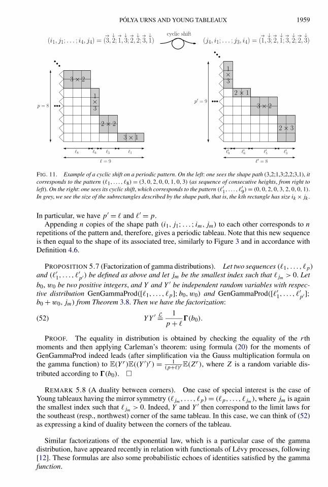
PÓLYA URNS AND YOUNG TABLEAUX 1959
FIG. 11. Example of a cyclic shift on a periodic pattern. On the left: one sees the shape path (3,2;1,3;2,2;3,1), itcorresponds to the pattern (�1, . . . , �8) = (3,0,2,0,0,1,0,3) (as sequence of consecutive heights, from right toleft). On the right: one sees its cyclic shift, which corresponds to the pattern (�′
1, . . . , �′9) = (0,0,2,0,3,2,0,0,1).
In grey, we see the size of the subrectangles described by the shape path, that is, the kth rectangle has size ik × jk .
In particular, we have p′ = � and �′ = p.Appending n copies of the shape path (i1, j1; . . . ; im, jm) to each other corresponds to n
repetitions of the pattern and, therefore, gives a periodic tableau. Note that this new sequenceis then equal to the shape of its associated tree, similarly to Figure 3 and in accordance withDefinition 4.6.
PROPOSITION 5.7 (Factorization of gamma distributions). Let two sequences (�1, . . . , �p)
and (�′1, . . . , �
′p′) be defined as above and let jm be the smallest index such that �jm > 0. Let
b0, w0 be two positive integers, and Y and Y ′ be independent random variables with respec-tive distribution GenGammaProd([�1, . . . , �p];b0,w0) and GenGammaProd([�′
1, . . . , �′p′ ];
b0 + w0, jm) from Theorem 3.8. Then we have the factorization:
(52) YY ′ L= 1
p + ��(b0).
PROOF. The equality in distribution is obtained by checking the equality of the r thmoments and then applying Carleman’s theorem: using formula (20) for the moments ofGenGammaProd indeed leads (after simplification via the Gauss multiplication formula onthe gamma function) to E(Y r)E((Y ′)r ) = 1
(p+�)rE(Zr), where Z is a random variable dis-
tributed according to �(b0). �
REMARK 5.8 (A duality between corners). One case of special interest is the case ofYoung tableaux having the mirror symmetry (�jm, . . . , �p) = (�p, . . . , �jm), where jm is againthe smallest index such that �jm > 0. Indeed, Y and Y ′ then correspond to the limit laws forthe southeast (resp., northwest) corner of the same tableau. In this case, we can think of (52)as expressing a kind of duality between the corners of the tableau.
Similar factorizations of the exponential law, which is a particular case of the gammadistribution, have appeared recently in relation with functionals of Lévy processes, following[12]. These formulas are also some probabilistic echoes of identities satisfied by the gammafunction.
1960 C. BANDERIER, P. MARCHAL AND M. WALLNER
We can mention one last result in this direction: indeed, Theorem 4.23 used for the Youngtableau with periodic pattern shape (�1, . . . , �p;2n) and the (same) Young tableau with peri-odic pattern shape (�1, . . . , �p, �1, . . . , �p;n) leads to two different closed forms of the samelimit distribution, and one also gets other closed forms if one repeats m times the pattern(�1, . . . , �p). For example, if one takes all the �′
is equal to 1, this gives
GenGamma(3,2) = √2 GenGamma(3,4)GenGamma(5,4),
and, more generally,
GenGamma(s0 + 1,2) = √m
m∏k=1
GenGamma(s0 + 2k − 1,2m).
Using the fact that GenGamma(a,1/b) = �(ab)b, we can rephrase this identity in terms ofpowers of � distributions (the notation �, in bold, stands for the distribution, while � standsfor the function; below, we have only occurrences in bold):
�
(s0 + 1
2
) 12 = √
m
m∏k=1
�
(s0 + 2k − 1
2m
) 12m
.
With x := s0+12m
, one gets the following formula equivalent to the Gauss multiplication for-mula:
�(mx)m = mmm∏
k=1
�
(x + k − 1
m
).
Choosing other values for the �i ’s leads to more identities:
p+�−1∏i=1
i �=�1+···+�j+j
with 1≤j≤p−1
GenGamma(s0 + i, p + �)
= m1−δm(p+�)−1∏
i=1i �=�′
1+···+�′j+j
with 1≤j≤mp−1
GenGamma(s0 + i,m(p + �)
).
It is pleasant that it is possible to reverse engineer such identities, and thus obtain a proba-bilistic proof of the Gauss multiplication formula (see [24]).
This ends our journey in the realm of urns and Young tableaux; in the next final section,we conclude with a few words on possible extensions of the methods used in this article.
A method is a trick used twice.George Pólya (1887–1985)
After this the reader who wishes to do so will have no difficulty in developing the theory of urns12
when they are regarded as differential operators.Alfred Young (1873–1940)
12The reader is invited to compare with the original citations of Pólya and Young in [75], page 208, and [38],page 366.

PÓLYA URNS AND YOUNG TABLEAUX 1961
6. Conclusion and further work. In this article, we introduced Pólya urns with periodicreplacements and showed that they can be exactly solved with generating function techniques.The initial partial differential equation encoding their dynamics leads to D-finite momentgenerating functions, which we identify as the signature of a generalized gamma productdistribution. It is also pleasant that it finds applications for some statistics of Young tableaux.
Many extensions of this work are possible:
• The density method which we introduced in [10, 64] can be used to analyse other combi-natorial structures, like we did already on permutations, trees, Young tableaux and Youngtableaux with local decreases. In fact, the idea to use integral representations of orderpolytope volumes in order to enumerate poset structures is quite natural, and was used, forexample, in [11, 28, 69]. Our approach, which uses this idea while following at the sametime the densities of some parameter, allows us to solve both enumeration and randomgeneration. We hope that some readers will give it a try on their favourite poset structure.
• In [31], Flajolet et al. analyse an urn model which leads to a remarkably simple factor-ization for the history generating function; see Theorem 1 therein and also Theorem 1 in[30]. This greatly helps them to perform the asymptotic analysis via analytic combina-torics tools. Our model does not possess such a factorization; this makes the proofs moreinvolved. It is nice that our new approach remains generic and can be applied to moregeneral periodic urn models (with weights, negative entries, random entries, unbalancedschemes, triangular urns with more colours, multiple drawings, . . . ). It is a full programmeto investigate these variants, in order to get a better characterization of the zoo of specialfunctions (combination of generalized hypergeometric, etc.) and distributions occurringfor the different models.
• There exists a theory of elimination for partial differential equations, chiefly developed inthe 1920s by Janet, Riquier and Thomas (see, e.g., [16, 35] for modern approaches). In ourcase, these approaches however fail to get the linear ordinary differential equations satisfiedby our generating functions. It is thus an interesting challenge for computer algebra to getan efficient algorithm taking as input the PDE and its boundary conditions, and giving asoutput the D-finite equation (if any). Is it possible to extend holonomy theory beyond itsapparent linear frontiers? (See the last part of [71].) Also, as an extension of Remark 2.5, itis natural to ask: is it possible to extend the work of Flajolet and Lafforgue to the full classof D-finite equations, thus exhibiting new universal limit laws like we did here?
• Our approach can also be used to analyse the fluctuations of further cells in a randomYoung tableau. It remains a challenge to understand the full asymptotic landscape of sur-faces associated with random Young tableaux, even if it could be globally expected thatthey behave like a Gaussian free field, like many other random surfaces [51]. Understand-ing the fluctuations and the universality of the critical exponent at the corner could helpto get a more global picture. The Arctic circle phenomenon (see [80]) and the study ofthe level lines C in random Young tableaux and their possible limits in distribution, asdiscussed in Section 5.2, seems to be an interesting but very challenging problem.
Acknowledgements. Let us thank Vadim Gorin, Markus Kuba, Cécile Mailler and Hen-ning Sulzbach for kind exchanges on their work [37, 56, 58] and on related questions. We alsothank the referees of the preliminary AofA’2018 version [9] and of this Annals of Probabilityversion for their careful reading and suggestions which improved the quality of our paper.We also thank the organizers (Igor Pak, Alejandro Morales, Greta Panova and Dan Romik)of the meeting Asymptotic Algebraic Combinatorics (Banff, 11–15 March 2019) where wegot the opportunity to present this work.
Michael Wallner was supported by a MathStic funding from the University Paris NordSeptember–December 2017 and the Erwin Schrödinger Fellowship of the Austrian ScienceFund (FWF): J 4162-N35.
1962 C. BANDERIER, P. MARCHAL AND M. WALLNER
REFERENCES
[1] ABRAMOWITZ, M. and STEGUN, I. A., eds. (1984). Handbook of Mathematical Functions with Formulas,Graphs, and Mathematical Tables. A Wiley-Interscience Publication. Wiley, New York. Reprint of the1972 edition, Selected Government Publications. MR0757537
[2] ALDOUS, D. and DIACONIS, P. (1999). Longest increasing subsequences: From patience sortingto the Baik–Deift–Johansson theorem. Bull. Amer. Math. Soc. (N.S.) 36 413–432. MR1694204https://doi.org/10.1090/S0273-0979-99-00796-X
[3] ANDREWS, G. E., ASKEY, R. and ROY, R. (1999). Special Functions. Encyclopedia of Mathematicsand Its Applications 71. Cambridge Univ. Press, Cambridge. MR1688958 https://doi.org/10.1017/CBO9781107325937
[4] ANGEL, O., HOLROYD, A. E., ROMIK, D. and VIRÁG, B. (2007). Random sorting networks. Adv. Math.215 839–868. MR2355610 https://doi.org/10.1016/j.aim.2007.05.019
[5] ATHREYA, K. B. and KARLIN, S. (1968). Embedding of urn schemes into continuous time Markovbranching processes and related limit theorems. Ann. Math. Stat. 39 1801–1817. MR0232455https://doi.org/10.1214/aoms/1177698013
[6] ATHREYA, K. B. and NEY, P. E. (2004). Branching Processes. Dover, Mineola, NY. Reprint of the 1972original [Springer, New York; MR0373040]. MR2047480
[7] BAGCHI, A. and PAL, A. K. (1985). Asymptotic normality in the generalized Pólya–Eggenberger urnmodel, with an application to computer data structures. SIAM J. Algebr. Discrete Methods 6 394–405.MR0791169 https://doi.org/10.1137/0606041
[8] BANDERIER, C. and DRMOTA, M. (2015). Formulae and asymptotics for coefficients of algebraic functions.Combin. Probab. Comput. 24 1–53. MR3318039 https://doi.org/10.1017/S0963548314000728
[9] BANDERIER, C., MARCHAL, P. and WALLNER, M. (2018). Periodic Pólya urns and an application toYoung tableaux. In 29th International Conference on Probabilistic, Combinatorial and AsymptoticMethods for the Analysis of Algorithms. LIPIcs. Leibniz Int. Proc. Inform. 110 Art. No. 11, 13. SchlossDagstuhl. Leibniz-Zent. Inform., Wadern. MR3826130
[10] BANDERIER, C., MARCHAL, P. and WALLNER, M. (2018). Rectangular Young tableaux with local de-creases and the density method for uniform random generation. In GASCom 2018, CEUR WorkshopProceedings 2113 60–68.
[11] BARYSHNIKOV, Y. and ROMIK, D. (2010). Enumeration formulas for Young tableaux in a diagonal strip.Israel J. Math. 178 157–186. MR2733067 https://doi.org/10.1007/s11856-010-0061-6
[12] BERTOIN, J. and YOR, M. (2001). On subordinators, self-similar Markov processes and some factorizationsof the exponential variable. Electron. Commun. Probab. 6 95–106. MR1871698 https://doi.org/10.1214/ECP.v6-1039
[13] BIANE, P. (1998). Representations of symmetric groups and free probability. Adv. Math. 138 126–181.MR1644993 https://doi.org/10.1006/aima.1998.1745
[14] BORODIN, A. and OLSHANSKI, G. (2017). Representations of the Infinite Symmetric Group. Cam-bridge Studies in Advanced Mathematics 160. Cambridge Univ. Press, Cambridge. MR3618143https://doi.org/10.1017/CBO9781316798577
[15] BOSTAN, A., CHYZAK, F., GIUSTI, M., LEBRETON, R., LECERF, G., SALVY, B. and SCHOST, É. (2017).Algorithmes Efficaces en Calcul Formel. Self-publishing.
[16] BOULIER, F., LEMAIRE, F., POTEAUX, A. and MORENO MAZA, M. (2019). An equivalence theorem forregular differential chains. J. Symbolic Comput. 93 34–55. MR3913563 https://doi.org/10.1016/j.jsc.2018.04.011
[17] BOUTILLIER, C., BOUTTIER, J., CHAPUY, G., CORTEEL, S. and RAMASSAMY, S. (2017). Dimers on railyard graphs. Ann. Inst. Henri Poincaré D 4 479–539. MR3734415 https://doi.org/10.4171/AIHPD/46
[18] BOUTTIER, J., CHAPUY, G. and CORTEEL, S. (2017). From Aztec diamonds to pyramids: Steep tilings.Trans. Amer. Math. Soc. 369 5921–5959. MR3646784 https://doi.org/10.1090/tran/7169
[19] BUBECK, S., MOSSEL, E. and RÁCZ, M. Z. (2015). On the influence of the seed graph in the preferentialattachment model. IEEE Trans. Netw. Sci. Eng. 2 30–39. MR3361606 https://doi.org/10.1109/TNSE.2015.2397592
[20] BUFETOV, A. and GORIN, V. (2019). Fourier transform on high-dimensional unitary groups with ap-plications to random tilings. Duke Math. J. 168 2559–2649. MR4007600 https://doi.org/10.1215/00127094-2019-0023
[21] CARLEMAN, T. (1923). Sur les équations intégrales singulières à noyau réel et symétrique. Uppsala Uni-versitets Årsskrift.
[22] CHAUVIN, B., MAILLER, C. and POUYANNE, N. (2015). Smoothing equations for large Pólya urns. J. The-oret. Probab. 28 923–957. MR3413961 https://doi.org/10.1007/s10959-013-0530-z
PÓLYA URNS AND YOUNG TABLEAUX 1963
[23] DEVROYE, L. (1986). Nonuniform Random Variate Generation. Springer, New York. MR0836973https://doi.org/10.1007/978-1-4613-8643-8
[24] DUFRESNE, D. (2010). G distributions and the beta-gamma algebra. Electron. J. Probab. 15 2163–2199.MR2745729 https://doi.org/10.1214/EJP.v15-845
[25] DUSE, E., JOHANSSON, K. and METCALFE, A. (2016). The cusp-Airy process. Electron. J. Probab. 21Paper No. 57, 50. MR3546394 https://doi.org/10.1214/16-EJP2
[26] EGGENBERGER, F. and PÓLYA, G. (1923). Über die Statistik verketteter Vorgänge. ZAMM Z. Angew. Math.Mech. 3 279–290. https://doi.org/10.1002/zamm.19230030407
[27] EGGENBERGER, F. and PÓLYA, G. (1928). Sur l’interprétation de certaines courbes de fréquence. C. R.Acad. Sci. 187 870–872.
[28] ELKIES, N. D. (2003). On the sums∑∞
k=−∞(4k + 1)−n. Amer. Math. Monthly 110 561–573. MR2001148https://doi.org/10.2307/3647742
[29] FANTI, G. and VISWANATH, P. (2017). Deanonymization in the Bitcoin P2P network. In Proceedings ofthe 31st Conference on Neural Information Processing Systems.
[30] FLAJOLET, P., DUMAS, P. and PUYHAUBERT, V. (2006). Some exactly solvable models of urn process the-ory. In Fourth Colloquium on Mathematics and Computer Science Algorithms, Trees, Combinatoricsand Probabilities. Discrete Math. Theor. Comput. Sci. Proc., AG 59–118. Assoc. Discrete Math. Theor.Comput. Sci., Nancy. MR2509623
[31] FLAJOLET, P., GABARRÓ, J. and PEKARI, H. (2005). Analytic urns. Ann. Probab. 33 1200–1233.MR2135318 https://doi.org/10.1214/009117905000000026
[32] FLAJOLET, P. and LAFFORGUE, T. (1994). Search costs in quadtrees and singularity perturbation asymp-totics. Discrete Comput. Geom. 12 151–175. MR1283884 https://doi.org/10.1007/BF02574372
[33] FLAJOLET, P. and SEDGEWICK, R. (2009). Analytic Combinatorics. Cambridge Univ. Press, Cambridge.MR2483235 https://doi.org/10.1017/CBO9780511801655
[34] FRÉCHET, M. and SHOHAT, J. (1931). A proof of the generalized second-limit theorem in the theory ofprobability. Trans. Amer. Math. Soc. 33 533–543. MR1501604 https://doi.org/10.2307/1989421
[35] GERDT, V. P., LANGE-HEGERMANN, M. and ROBERTZ, D. (2019). The MAPLE package TDDS forcomputing Thomas decompositions of systems of nonlinear PDEs. Comput. Phys. Commun. 234 202–215. MR3864422 https://doi.org/10.1016/j.cpc.2018.07.025
[36] GOLDSCHMIDT, C. and HAAS, B. (2015). A line-breaking construction of the stable trees. Electron. J.Probab. 20 no. 16, 24. MR3317158 https://doi.org/10.1214/EJP.v20-3690
[37] GORIN, V. and RAHMAN, M. (2019). Random sorting networks: Local statistics via random matrix laws.Probab. Theory Related Fields 175 45–96. MR4009705 https://doi.org/10.1007/s00440-018-0886-1
[38] GRACE, J. H. and YOUNG, A. (2010). The Algebra of Invariants. Cambridge Library Collection. Cam-bridge Univ. Press, Cambridge. Reprint of the 1903 original. MR2850282 https://doi.org/10.1017/CBO9780511708534
[39] GRAHAM, R. L., KNUTH, D. E. and PATASHNIK, O. (1994). Concrete Mathematics: A Foundation forComputer Science, 2nd ed. Addison-Wesley, Reading, MA. MR1397498
[40] GREENE, C., NIJENHUIS, A. and WILF, H. S. (1984). Another probabilistic method in the theory of Youngtableaux. J. Combin. Theory Ser. A 37 127–135. MR0757611 https://doi.org/10.1016/0097-3165(84)90065-7
[41] HAN, G.-N. (2010). New hook length formulas for binary trees. Combinatorica 30 253–256. MR2676840https://doi.org/10.1007/s00493-010-2503-5
[42] HWANG, H.-K., KUBA, M. and PANHOLZER, A. (2007). Analysis of some exactly solvable diminishingurn models. In Proceedings of FPSAC’2007 (Formal Power Series and Algebraic Combinatorics).Nankai Univ., Tianjin.
[43] JANSON, S. (2004). Functional limit theorems for multitype branching processes and generalized Pólyaurns. Stochastic Process. Appl. 110 177–245. MR2040966 https://doi.org/10.1016/j.spa.2003.12.002
[44] JANSON, S. (2005). Asymptotic degree distribution in random recursive trees. Random Structures Algo-rithms 26 69–83. MR2116576 https://doi.org/10.1002/rsa.20046
[45] JANSON, S. (2006). Limit theorems for triangular urn schemes. Probab. Theory Related Fields 134 417–452.MR2226887 https://doi.org/10.1007/s00440-005-0442-7
[46] JANSON, S. (2007). Brownian excursion area, Wright’s constants in graph enumeration, and other Brownianareas. Probab. Surv. 4 80–145. MR2318402 https://doi.org/10.1214/07-PS104
[47] JANSON, S. (2010). Moments of gamma type and the Brownian supremum process area. Probab. Surv. 71–52. MR2645216 https://doi.org/10.1214/10-PS160
[48] JOHANSSON, K. and NORDENSTAM, E. (2006). Eigenvalues of GUE minors. Electron. J. Probab. 11 1342–1371. MR2268547 https://doi.org/10.1214/EJP.v11-370
[49] KAHANE, J.-P. (1960). Propriétés locales des fonctions à séries de Fourier aléatoires. Studia Math. 19 1–25.MR0117506 https://doi.org/10.4064/sm-19-1-1-25

1964 C. BANDERIER, P. MARCHAL AND M. WALLNER
[50] KAUERS, M. and PAULE, P. (2011). The Concrete Tetrahedron: Symbolic Sums, Recurrence Equa-tions, Generating Functions, Asymptotic Estimates. Texts and Monographs in Symbolic Computation.Springer, Vienna. MR2768529 https://doi.org/10.1007/978-3-7091-0445-3
[51] KENYON, R. (2001). Dominos and the Gaussian free field. Ann. Probab. 29 1128–1137. MR1872739https://doi.org/10.1214/aop/1015345599
[52] KEROV, S. V. (1993). Transition probabilities of continual Young diagrams and the Markov moment prob-lem. Funct. Anal. Appl. 27 104–117. https://doi.org/10.1007/BF01085981
[53] KHODABIN, M. and AHMADABADI, A. (2010). Some properties of generalized gamma distribution. Math.Sci. 4 9–27. MR2673499
[54] KUBA, M. and MAHMOUD, H. M. (2017). Two-color balanced affine urn models with multiple drawings.Adv. in Appl. Math. 90 1–26. MR3666709 https://doi.org/10.1016/j.aam.2017.04.004
[55] KUBA, M. and PANHOLZER, A. (2016). Combinatorial families of multilabelled increasing trees and hook-length formulas. Discrete Math. 339 227–254. MR3404485 https://doi.org/10.1016/j.disc.2015.08.010
[56] KUBA, M. and SULZBACH, H. (2017). On martingale tail sums in affine two-color urn models with multipledrawings. J. Appl. Probab. 54 96–117. MR3632608 https://doi.org/10.1017/jpr.2016.89
[57] LAH, I. (1954). A new kind of numbers and its application in the actuarial mathematics. Bol. Inst. DosActuár. Portugueses 9 7–15.
[58] LASMAR, N., MAILLER, C. and SELMI, O. (2018). Multiple drawing multi-colour urns by stochastic ap-proximation. J. Appl. Probab. 55 254–281. MR3780393 https://doi.org/10.1017/jpr.2018.16
[59] LINUSSON, S., POTKA, S. and SULZGRUBER, R. (2018). On random shifted standard Young tableaux and132-avoiding sorting networks. Available at arXiv:1804.01795.
[60] LOGAN, B. F. and SHEPP, L. A. (1977). A variational problem for random Young tableaux. Adv. Math. 26206–222. MR1417317 https://doi.org/10.1016/0001-8708(77)90030-5
[61] MACDONALD, I. G. (2015). Symmetric Functions and Hall Polynomials, 2nd ed. Oxford Classic Texts inthe Physical Sciences. Clarendon, Oxford. With contribution by A. V. Zelevinsky and a foreword byRichard Stanley. Reprint of the 2008 paperback edition [MR1354144]. MR3443860
[62] MAHMOUD, H. M. (2009). Pólya Urn Models. Texts in Statistical Science Series. CRC Press, Boca Raton,FL. MR2435823
[63] MARCHAL, P. (2016). Rectangular Young tableaux and the Jacobi ensemble. Discrete Math. Theor. Comput.Sci. Proc. BC 839–850.
[64] MARCHAL, P. (2018). The density method for permutations with prescribed descents. In GASCom 2018,CEUR Workshop Proceedings 2113 179–186.
[65] MCKAY, B. D., MORSE, J. and WILF, H. S. (2002). The distributions of the entries of Young tableaux.J. Combin. Theory Ser. A 97 117–128. MR1879130 https://doi.org/10.1006/jcta.2001.3200
[66] MORALES, A. H., PAK, I. and PANOVA, G. (2019). Hook formulas for skew shapes III. Multivariate andproduct formulas. Algebraic Combin. 2 815–861. MR4023568
[67] MORCRETTE, B. and MAHMOUD, H. M. (2012). Exactly solvable balanced tenable urns with randomentries via the analytic methodology. In 23rd Intern. Meeting on Probabilistic, Combinatorial, andAsymptotic Methods for the Analysis of Algorithms (AofA’12). Discrete Math. Theor. Comput. Sci.Proc., AQ 219–232. Assoc. Discrete Math. Theor. Comput. Sci., Nancy. MR2957333
[68] OLVER, F. W. J., LOZIER, D. W., BOISVERT, R. F. and CLARK, C. W., eds. (2010). NIST Handbook ofMathematical Functions. U.S. Dept. Commerce, National Institute of Standards and Technology. Seealso the NIST Digital Library of Mathematical Functions.
[69] PAK, I. (2001/02). Hook length formula and geometric combinatorics. Sém. Lothar. Combin. 46 Art. B46f,13. MR1877632
[70] PEKÖZ, E. A., RÖLLIN, A. and ROSS, N. (2016). Generalized gamma approximation with rates for urns,walks and trees. Ann. Probab. 44 1776–1816. MR3502594 https://doi.org/10.1214/15-AOP1010
[71] PETKOVŠEK, M., WILF, H. S. and ZEILBERGER, D. (1996). A = B . AK Peters, Wellesley.[72] PETROV, L. (2015). Asymptotics of uniformly random lozenge tilings of polygons. Gaussian free field. Ann.
Probab. 43 1–43. MR3298467 https://doi.org/10.1214/12-AOP823[73] PITTEL, B. and ROMIK, D. (2007). Limit shapes for random square Young tableaux. Adv. in Appl. Math.
38 164–209. MR2290809 https://doi.org/10.1016/j.aam.2005.12.005[74] PÓLYA, G. (1930). Sur quelques points de la théorie des probabilités. Ann. Inst. Henri Poincaré 1 117–161.
MR1507985[75] POLYA, G. (2014). How to Solve It: A New Aspect of Mathematical Method. Princeton Science Library.
Princeton Univ. Press, Princeton, NJ. With a foreword by John H. Conway. Reprint of the 1957 secondedition [MR2183670]. MR3289212
[76] PRUDNIKOV, A. P., BRYCHKOV, Y. A. and MARICHEV, O. I. (1992). Integrals and Series. Vol. 4: DirectLaplace Transforms. Gordon & Breach, New York.
PÓLYA URNS AND YOUNG TABLEAUX 1965
[77] RIORDAN, J. (2002). An Introduction to Combinatorial Analysis. Dover, Mineola, NY. Reprint of the 1958original [Wiley, New York; MR0096594 (20 #3077)]. MR1949650
[78] RIVEST, R. L. (2018). Bayesian tabulation audits: Explained and extended. Available at arXiv:1801.00528.[79] ROMIK, D. (2004). Explicit formulas for hook walks on continual Young diagrams. Adv. in Appl. Math. 32
625–654. MR2053837 https://doi.org/10.1016/S0196-8858(03)00096-4[80] ROMIK, D. (2012). Arctic circles, domino tilings and square Young tableaux. Ann. Probab. 40 611–647.
MR2952086 https://doi.org/10.1214/10-AOP628[81] ROMIK, D. (2015). The Surprising Mathematics of Longest Increasing Subsequences. Institute of Mathe-
matical Statistics Textbooks 4. Cambridge Univ. Press, New York. MR3468738[82] SAGAN, B. E. and YEH, Y. N. (1989). Probabilistic algorithms for trees. Fibonacci Quart. 27 201–208.
MR1002062[83] SALVY, B. and ZIMMERMANN, P. (1994). Gfun: A Maple package for the manipulation of generating and
holonomic functions in one variable. ACM Trans. Math. Software 20 163–177. https://doi.org/10.1145/178365.178368
[84] SÉNIZERGUES, D. (2019). Geometry of weighted recursive and affine preferential attachment trees. Avail-able at arXiv:1904.07115.
[85] SHEFFIELD, S. (2005). Random surfaces. Astérisque 304 vi+175. MR2251117[86] SNIADY, P. (2014). Robinson–Schensted–Knuth algorithm, jeu de taquin, and Kerov–Vershik measures on
infinite tableaux. SIAM J. Discrete Math. 28 598–630. MR3190750 https://doi.org/10.1137/130930169[87] STACY, E. W. (1962). A generalization of the gamma distribution. Ann. Math. Stat. 33 1187–1192.
MR0143277 https://doi.org/10.1214/aoms/1177704481[88] STANLEY, R. P. (1986). Two poset polytopes. Discrete Comput. Geom. 1 9–23. MR0824105
https://doi.org/10.1007/BF02187680[89] STANLEY, R. P. (1999). Enumerative Combinatorics. Vol. 2. Cambridge Studies in Advanced Mathematics
62. Cambridge Univ. Press, Cambridge. MR1676282 https://doi.org/10.1017/CBO9780511609589[90] VERSHIK, A. M. (2001). Randomization of algebra and algebraization of probability—an attempt at pre-
diction. In Mathematics Unlimited—2001 and Beyond 1157–1166. Springer, Berlin. MR1852209[91] VERŠIK, A. M. and KEROV, S. V. (1977). Asymptotic behavior of the Plancherel measure of the symmetric
group and the limit form of Young tableaux. Dokl. Akad. Nauk SSSR 233 1024–1027. MR0480398[92] WALL, H. S. (1948). Analytic Theory of Continued Fractions. Van Nostrand, New York, NY. MR0025596[93] WALLNER, M. (2020). A half-normal distribution scheme for generating functions. European J. Combin.
87 103–138. MR4090824 https://doi.org/10.1016/j.ejc.2020.103138