Universitat LeipzigFakultat fur Mathematik und Informatik

Mathematisches Institut

Periods and Algebraic deRham Cohomology

Diplomarbeitim Studiengang Diplom-Mathematik

Leipzig, vorgelegt von Benjamin Friedrich,geboren am 22. Juli 1979

Abstract

It is known that the algebraic deRham cohomology group HidR(X0/Q) of a nonsin-

gular variety X0/Q has the same rank as the rational singular cohomology groupHi

sing(Xan; Q) of the complex manifold Xan associated to the base change X0 ×Q C.

However, we do not have a natural isomorphism HidR(X0/Q) ∼= Hi

sing(Xan; Q). Any

choice of such an isomorphism produces certain integrals, so called periods, whichreveal valuable information about X0. The aim of this thesis is to explain these clas-sical facts in detail. Based on an approach of Kontsevich [K, pp. 62–64], differentdefinitions of a period are compared and their properties discussed. Finally, the the-ory is applied to some examples. These examples include a representation of ζ(2) asa period and a variation of mixed Hodge structures used by Goncharov [G1].

Contents

1 Introduction 1

2 The Associated Complex Analytic Space 42.1 The Definition of the Associated Complex Analytic Space . . . . . . . 42.2 Algebraic and Analytic Coherent Sheaves . . . . . . . . . . . . . . . . 5

3 Algebraic deRham Theory 103.1 Classical deRham Cohomology . . . . . . . . . . . . . . . . . . . . . . 103.2 Algebraic deRham Cohomology . . . . . . . . . . . . . . . . . . . . . . 123.3 Basic Lemmas . . . . . . . . . . . . . . . . . . . . . . . . . . . . . . . . 153.4 The Long Exact Sequence in Algebraic deRham Cohomology . . . . . 163.5 Behaviour Under Base Change . . . . . . . . . . . . . . . . . . . . . . 173.6 Some Spectral Sequences . . . . . . . . . . . . . . . . . . . . . . . . . . 18

4 Comparison Isomorphisms 244.1 Situation . . . . . . . . . . . . . . . . . . . . . . . . . . . . . . . . . . 244.2 Analytic deRham Cohomology . . . . . . . . . . . . . . . . . . . . . . 244.3 The Long Exact Sequence in Analytic deRham Cohomology . . . . . . 254.4 Some Spectral Sequences for Analytic deRham Cohomology . . . . . . 254.5 Comparison of Algebraic and Analytic deRham Cohomology . . . . . 264.6 Complex Cohomology . . . . . . . . . . . . . . . . . . . . . . . . . . . 284.7 Comparison of Analytic deRham Cohomology and Complex Cohomology 304.8 Singular Cohomology . . . . . . . . . . . . . . . . . . . . . . . . . . . . 324.9 Comparison of Complex Cohomology and Singular Cohomology . . . . 334.10 Comparison Theorem . . . . . . . . . . . . . . . . . . . . . . . . . . . 334.11 An Alternative Description of the Comparison Isomorphism . . . . . . 344.12 A Motivation for the Theory of Periods . . . . . . . . . . . . . . . . . 41

5 Definitions of Periods 435.1 First Definition of a Period: Pairing Periods . . . . . . . . . . . . . . . 435.2 Second Definition of a Period: Abstract Periods . . . . . . . . . . . . . 445.3 Third Definition of a Period: Naıve Periods . . . . . . . . . . . . . . . 46

6 Triangulation of Algebraic Varieties 496.1 Semi-algebraic Sets . . . . . . . . . . . . . . . . . . . . . . . . . . . . . 496.2 Semi-algebraic Singular Chains . . . . . . . . . . . . . . . . . . . . . . 53

7 Periods Revisited 577.1 Comparison of Definitions of Periods . . . . . . . . . . . . . . . . . . . 577.2 Torsors . . . . . . . . . . . . . . . . . . . . . . . . . . . . . . . . . . . 627.3 Fourth Definition of a Period: Effective Periods . . . . . . . . . . . . . 63

8 Examples 678.1 First Example: A1

C \ 0 . . . . . . . . . . . . . . . . . . . . . . . . . . 678.2 Second Example: Quadratic Forms . . . . . . . . . . . . . . . . . . . . 708.3 Third Example: Elliptic Curves . . . . . . . . . . . . . . . . . . . . . . 728.4 Fourth Example: A ζ-value . . . . . . . . . . . . . . . . . . . . . . . . 758.5 Fifth Example: The Double Logarithm Variation of Mixed Hodge

Structures . . . . . . . . . . . . . . . . . . . . . . . . . . . . . . . . . . 77

A Sign Conventions and Related Material 94

1 Introduction

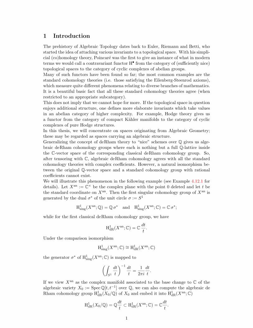
The prehistory of Algebraic Topology dates back to Euler, Riemann and Betti, whostarted the idea of attaching various invariants to a topological space. With his simpli-cial (co)homology theory, Poincare was the first to give an instance of what in modernterms we would call a contravariant functor H• from the category of (sufficiently nice)topological spaces to the category of cyclic complexes of abelian groups.Many of such functors have been found so far; the most common examples are thestandard cohomology theories (i.e. those satisfying the Eilenberg-Steenrod axioms),which measure quite different phenomena relating to diverse branches of mathematics.It is a beautiful basic fact that all these standard cohomology theories agree (whenrestricted to an appropriate subcategory).This does not imply that we cannot hope for more. If the topological space in questionenjoys additional structure, one defines more elaborate invariants which take valuesin an abelian category of higher complexity. For example, Hodge theory gives usa functor from the category of compact Kahler manifolds to the category of cycliccomplexes of pure Hodge structures.In this thesis, we will concentrate on spaces originating from Algebraic Geometry;these may be regarded as spaces carrying an algebraic structure.Generalizing the concept of deRham theory to “nice” schemes over Q gives us alge-braic deRham cohomology groups where each is nothing but a full Q-lattice insidethe C-vector space of the corresponding classical deRham cohomology group. So,after tensoring with C, algebraic deRham cohomology agrees with all the standardcohomology theories with complex coefficients. However, a natural isomorphism be-tween the original Q-vector space and a standard cohomology group with rationalcoefficients cannot exist.We will illustrate this phenomenon in the following example (see Example 4.12.1 fordetails). Let Xan := C× be the complex plane with the point 0 deleted and let t bethe standard coordinate on Xan. Then the first singular cohomology group of Xan isgenerated by the dual σ∗ of the unit circle σ := S1

H1sing(X

an; Q) = Qσ∗ and H1sing(X

an; C) = Cσ∗;

while for the first classical deRham cohomology group, we have

H1dR(Xan; C) = C

dt

t.

Under the comparison isomorphism

H1sing(X

an; C) ∼= H1dR(Xan; C)

the generator σ∗ of H1sing(X

an; C) is mapped to(∫S1

dt

t

)−1 dt

t=

12πi

dt

t.

If we view Xan as the complex manifold associated to the base change to C of thealgebraic variety X0 := Spec Q[t, t−1] over Q, we can also compute the algebraic deRham cohomology group H1

dR(X0/Q) of X0 and embed it into H1dR(Xan; C)

H1dR(X0/Q) = Q

dt

t⊂ H1

dR(Xan; C) = Cdt

t.

1

Thus we get two Q-lattices inside H1dR(Xan; C), H1

sing(Xan; Q) and H1

dR(X0/Q), whichdo not coincide. In fact, they differ by the factor 2πi — our first example of what wewill call a period. Other examples will produce period numbers like π, ln 2, ellipticintegrals, or ζ(2), which are interesting also from a number theoretical point of view(cf. page 47).There is some ambiguity about the precise definition of a period; actually we will givefour definitions in total:

(i) pairing periods (cf. Definition 5.1.1 on page 43)

(ii) abstract periods (cf. Definition 5.2.1 on page 45)

(iii) naıve periods (cf. Definition 5.3.2 on page 46)

(iv) effective periods (cf. Definition 7.3.1 on page 63)

For X0 a nonsingular variety over Q, we have a natural pairing between the i th

algebraic deRham cohomology of X0 and the i th singular homology group of thecomplex manifold Xan associated to the base change X0 ×Q C

Hsingi (Xan; Q)×Hi

dR(X0/Q) −→ C.

The numbers which can appear in the image of this pairing (or its version for relativecohomology) are called pairing periods; this is the most traditional way to define aperiod.In [K, p. 62], Kontsevich gives the alternative definition of effective periods whichdoes not need algebraic deRham cohomology and, at least conjecturally, gives the setof all periods some extra algebraic structure. We present his ideas in Subsection 7.3.Abstract periods describe just a variant of Kontsevich’s definition. In fact, we have asurjection from the set of effective periods to the set of abstract ones (cf. page 65),which is conjectured to be an isomorphism.Naıve periods are defined in an elementary way and are used to provide a connectionbetween pairing periods and abstract periods.In Kontsevich’s paper [K, p. 63], it is used that the notion of pairing and abstractperiod coincide. The aim of this thesis is to show that the following implications holdtrue (cf. Theorem 7.1.1)

abstract period⇔ naıve period⇒ pairing period.

The thesis is organized as follows. The discussion of the various definitions of a periodmakes up the principal part of the work filling sections five to seven.Section two gives an introduction to complex analytic spaces. Additionally, weprovide the connection to Algebraic Geometry by defining the associated complexanalytic space of a variety.In Section three, we define algebraic deRham cohomology for pairs consisting of avariety and a divisor on it. We also give some working tools for this cohomology.The aim of Section four is to give a comparison theorem (Theorem 4.10.1) whichstates that algebraic deRham and singular cohomology agree.In Section five, we present the definition of pairing, abstract, and naıve periods andprove some of their properties.Section six provides some facts about the triangulation of algebraic varieties.

2

Section seven contains the main result (Theorem 7.1.1) about the implicationsbetween the various definitions of a period mentioned above. Furthermore, we givethe definition of effective periods which motivated the definition of abstract periods.In the last section, Section eight, we consider five examples to give an application ofthe general theory. Among them is a representation of ζ(2) as an abstract period andthe famous double logarithm variation of mixed Hodge structures used by Goncharov[G1] whose geometric origin is emphasized.

Conventions. By a variety, we will always mean a reduced, quasi-projective scheme.We will often deal with a variety X0 defined over some algebraic extension of Q. Asa rule, skipping the subscript 0 will always mean base change to C

X := “X0 ×Q C ” = X0 ×Spec Q Spec C.

(An exception is section three, where arbitrary base fields are used.) The complexanalytic space associated to X will be denoted by Xan (cf. Subsection 2.1).The sign conventions used throughout this thesis are listed in the appendix.

Acknowledgments. I am greatly indebted to my supervisor Prof. A. Huber-Klawitter for her guidance and her encouragement. I very much appreciated theinformal style of our discussions in which she vividly pointed out to me the centralideas of the mathematics involved.I would also like to thank my fellow students R. Munck, M. Witte and K. Zehmischwho read the manuscript and gave numerous comments which helped to clarify theexposition.

3

2 The Associated Complex Analytic Space

Let X be a variety over C. The set |X| of closed points of X inherits the Zariskitopology. However, we can also equip this set with the standard topology: For smoothX this gives a complex manifold; in general we get a complex analytic space Xan.The main reference for this section is [Ha, B.1].

2.1 The Definition of the Associated Complex Analytic Space

We consider an example before giving the general definition of a complex analyticspace.

Example 2.1.1. Let Dn ⊂ Cn be the polycylinder

Dn := z ∈ Cn | |zi| < 1, i = 1, . . . , n

andODn the sheaf of holomorphic functions onDn. For a set of holomorphic functionsf1, . . . , fm ∈ Γ(Dn,ODn) we define

XDn := z ∈ Dn | f1(z) = . . . = fm(z) = 0OXDn := ODn/(f1, . . . , fm).

(1)

The locally ringed space (XDn ,OXDn ) from this example is a complex analytic space.In general, complex analytic spaces are obtained by glueing spaces of the form (1).

Definition 2.1.2 (Complex analytic space, [Ha, B.1, p. 438]). A locally ringedspace (X ,OX ) is called complex analytic if it is locally (as a locally ringed space)isomorphic to one of the form (1). A morphism of complex analytic spaces is amorphism of locally ringed spaces.

For any scheme (X,OX) of finite type over C we have an associated complex analyticspace (Xan,OXan).

Definition 2.1.3 (Associated complex analytic space, [Ha, B.1, p. 439]).Assume first that X is affine. We fix an isomorphism

X ∼= Spec C[x1, . . . , xn]/(f1, . . . , fm)

and then consider the fi as holomorphic functions on Cn in order to set

Xan := z ∈ Cn | f1(z) = . . . = fm(z) = 0OXan := OCn/(f1, . . . , fm),

where OCn denotes the sheaf of holomorphic functions on Cn.For an arbitrary scheme X of finite type over C, we take a covering of X by openaffine subsets Ui. The scheme X is obtained by glueing the open sets Ui, so we canuse the same glueing data to glue the complex analytic space (Ui)an into an analyticspace Xan. This is the associated complex analytic space of X.

This construction is natural and we obtain a functor an from the category of schemesof finite type over C to the category of complex analytic spaces. Note that its re-striction to the subcategory of smooth schemes maps into the category of complexmanifolds as a consequence of the inverse function theorem (cf. [Gun, Thm. 6, p. 20]).

4

Example 2.1.4. The complex analytic space associated to complex projective spaceis again complex projective space, but considered as a complex manifold. To avoidconfusion in the subsequent sections, the notation CPn will be reserved for com-plex projective space in the category of schemes, whereas we write CPnan for complexprojective space in the category of complex analytic spaces.

For any scheme X of finite type over C, we have a natural map of locally ringedspaces

φ : Xan → X (2)

which induces the identity on the set of closed points |X| of X. Note that φ∗OX =OXan .

2.2 Algebraic and Analytic Coherent Sheaves

Let us consider sheaves of OX -modules. The equality of functors

Γ(X, ?) = Γ(Xan, φ−1?)

gives an equality of their right derived functors

Hi(X; ?) = RiΓ(X; ?) = RiΓ(Xan;φ−1?).

Since φ−1 is an exact functor, the spectral sequence for the composition of the functorsφ−1 and Γ(Xan; ?) degenerates and we obtain

Hi(Xan;φ−1?) = RiΓ(Xan; ?) φ−1 = RiΓ(Xan;φ−1?).

Thus the natural map for F a sheaf of OX -modules

φ−1F → φ∗F

gives a natural map of cohomology groups

Hi(X;F) = Hi(Xan;φ−1F)→ Hi(Xan;φ∗F). (3)

Sheaf cohomology behaves particularly nice for coherent sheaves, this notion beingdefined as follows.

Definition 2.2.1 (Coherent sheaf). We define a coherent sheaf F on X (resp.Xan) to be a sheaf of OX-modules (resp. OXan-modules) that is Zariski-locally (resp.locally in the standard topology) isomorphic to the cokernel of a morphism of freeOX-modules (resp. OXan-modules) of finite rank

OrU −→ OsU −→ F|U −→ 0, for U ⊆ X (resp. U ⊆ Xan) open, (4)

where r, s ∈ N.

For sheaves on X this agrees with the definition given in [Ha, II.5, p. 111]. For thisalternate definition, we need some notation: If U = SpecA is an affine variety andM an A-module, we denote by M the sheaf on U associated to M (i.e. the sheafassociated to the presheaf V 7→ Γ(V ;OV ) ⊗A M for V ⊆ U open, see [Ha, II.5, p.110]).

5

Lemma 2.2.2 (cf. [Ha, II.5 Exercise 5.4, p. 124]). A sheaf F of OX-modulesis coherent if and only if X can be covered by open affine subsets Ui = SpecAi suchthat F|Ui

∼= Mi for some finitely generated Ai-modules Mi.

Proof. “if”: The Ai’s are Noetherian rings. Therefore any finitely generated Ai-module Mi will be finitely presented

Ari −→ Asi −→Mi −→ 0.

Since localization is an exact functor, we get

OrUi−→ OsUi

−→ Mi −→ 0,

which proves the “if”-part. “only if”: W.l.o.g. we may assume that the open subsets U ⊆ X in (4) are affineU = SpecA. Then Γ(U ;OU ) = A and OU = A. Now the A-module

M := coker(Γ(U ;OrU ) −→ Γ(U ;OsU )

)=coker(Ar −→ As)

is clearly finitely generated. Since

Ar −→ As −→M −→ 0

givesAr −→ As −→ M −→ 0,

we conclude

F|U = coker(OrU −→ OsU ) = coker(Ar −→ As) = M.

As an immediate consequence of the definition of a coherent sheaf F on X, we seethat the sheaf

Fan := φ∗F

will be coherent as well: If

OrU −→ OsU −→ F|U −→ 0

is exact, so isOrUan −→ OsUan −→ φ∗F|Uan −→ 0,

since φ−1 is exact and tensoring is a right exact functor.There is a famous theorem by Serre usually referred to as GAGA, since it is containedin his paper “Geometrie algebrique et geometrie analytique” [Se:gaga].

Theorem 2.2.3 (Serre, [Ha, B.2.1, p. 440]). Let X be a projective schemeover C. Then the map

F 7→ Fan

induces an equivalence between the category of coherent sheaves on X and the categoryof coherent sheaves on Xan. Furthermore, the natural map (3)

Hi(X;F) ∼−→ Hi(Xan;Fan)

is an isomorphism for all i.

6

Let us state a corollary of Theorem 2.2.3, which is not included in [Ha].

Corollary 2.2.4. In the situation of Theorem 2.2.3, we also have a natural isomor-phism for hypercohomology for all i

Hi(X;F•) ∼= Hi(Xan;F•an),

where F• is a bounded complex of coherent sheaves on X.

Here we only require the boundary morphisms of F• to be morphisms of sheaves ofabelian groups. They do not need to be OX -linear.Before we begin proving Corollary 2.2.4, we need some homological algebra.

Lemma 2.2.5. Let A be an abelian category and

F•[0] −→ G•,•, (5)

a morphism of double complexes of A-objects (cf. the appendix), where

• F•[0] is a double complex concentrated in the zeroth row with F• being acomplex vanishing below degree zero, i.e. Fn = 0 for n < 0, and

• G•,• is a double complex living only in non-negative degrees.

If for all q ∈ Z0→ Fq → G0,q → G1,q → · · ·

is a resolution of Fq, then the map of total complexes induced by (5)

F• ∼−→ totG•,•

is a quasi-isomorphism.

Proof. From (5) we obtain a morphism of spectral sequences

hpII hqI F•[0]⇒ hn F•

↓ ↓hpII hqI G•,• ⇒ hn totG•,•.

Both spectral sequences degenerate because of

hpII hqI F•[0] =

hp F• if q = 0,0 else

and

hpII hqI G•,• =

hp F• if q = 0,0 else

and so we get an isomorphism on the initial terms. Hence we also have an isomorphismon the limit terms and our assertion follows.

Remark 2.2.6. A similar statement holds with F•[0] considered as a double complexconcentrated in the zeroth column.

7

Godement resolutions. As we also need Γ-acyclic resolutions that behave functorialin the proof of Corollary 2.2.4, we now describe the concept of Godement resolutions.For any sheaf F on X (or Xan) define

g(F) :=∏x∈|X|

i∗Fx,

where i : x → X denotes the closed immersion of the point x. The sheaf g(F) isflabby and we have a natural inclusion

F g(F).

Setting Gi+1 := g(coker(Gi−1 → Gi)

)with G−1 := F and G0 := g(F) gives an exact

sequence0 −→ F −→ G0 −→ G1 −→ . . . .

We define the Godement resolution of F to be

G•F := 0 −→ G0 −→ G1 −→ . . . .

It is Γ-acyclic and functorial in F . Extending this definition to a bounded complexF•

G•,qF• := G•Fq

G•F• := totG•,•F•(6)

yields a map of double complexes

F•[0] −→ G•,•

and a quasi-isomorphism by Lemma 2.2.5

F• ∼−→ G•F• .

Let x ∈ |X| be a closed point of X. The map φ from (2) gives a commutative square

xan i→ Xan

φ ↓ ↓ φ

x i→ X

and a natural morphism (cf. [Ha, II.5, p. 110])

Fx −→ φ∗φ∗Fx,

where we consider the stalk Fx as a sheaf on x. This map induces another map

i∗Fx −→ i∗φ∗φ∗Fx = (i φ)∗φ∗Fx = (φ i)∗φ∗Fx = φ∗i∗φ

∗Fx,

and yet a third map (cf. loc. cit.)

ε : φ∗i∗Fx −→ i∗φ∗Fx, (7)

8

which is an isomorphism, as can be seen on the stalks

εx : φ∗Fx∼−→ φ∗Fx,

εy : 0 −→ 0, for y 6= x.

Consequently,

φ∗g(F) = φ∗∏x i∗Fx =

∏x φ∗i∗Fx

(7)=∏x i∗φ

∗Fx =∏x i∗(φ

∗F)x = g(φ∗Fx).

Thus we get firstφ∗G•Fp = G•φ∗Fp ,

thenφ∗G•F• = G•φ∗F• .

This gives us a natural map of hypercohomology groups

Hi(X;F•) = hiΓ(X;G•F•) = hiΓ(Xan;φ−1G•F•)−→

hiΓ(Xan;φ∗G•F•) = hiΓ(Xan;G•φ∗F•) = hiΓ(Xan;G•F•an

) = Hi(Xan;F•an). (8)

Proof of Corollary 2.2.4. We claim that the natural map (8) is an isomorphism forall i if X is projective.If F• has has length one, Theorem 2.2.3 tells us that this is indeed true. So let usassume that (8) is an isomorphism for all complexes of length ≤ n and let F• be acomplex of coherent sheaves on X of length n+ 1. W.l.o.g. Fn+1 6= 0 but Fp = 0 forp > n + 1. We write σ≤nF• for the complex F• cut off above degree n. The shortexact sequence

0 −→ Fn+1[−n− 1] −→ F• −→ σ≤nF• −→ 0

remains exact if we take the inverse image along φ

0 −→ Fn+1an [−n− 1] −→ F•an −→ σ≤nF•an −→ 0.

Using the naturality of (8), we obtain the following “ladder” with commuting squares

· · · → H−n−1+i(X;Fn+1) −−−−→ Hi(X;F•) −−−−→ Hi(X;σ≤nF•) → · · ·yo y yo· · · →H−n−1+i(Xan;Fn+1

an ) −−−−→ Hi(Xan;F•an) −−−−→ Hi(Xan;σ≤nF•an)→ · · ·

and the induction step follows from the 5-lemma.

9

3 Algebraic deRham Theory

In this section, we define the algebraic deRham cohomology H•dR(X,D/k) of a smoothvariety X over a field k and a normal-crossings-divisor D on X (cf. definitions 3.2.3,3.2.4, and 3.2.6). We also give some working tools for this cohomology: a basechange theorem (Proposition 3.5.1) and two spectral sequences (Corollary 3.6.3 andProposition 3.6.4).

3.1 Classical deRham Cohomology

This subsection only serves as a motivation for the following giving an overviewof classical deRham theory. For a complex manifold, analytic deRham, complex,and singular cohomology are defined and shown to be equal to classical deRhamcohomology. All material presented here will be generalized to a relative setup lateron.

Let M be a complex manifold. We recall two standard exact sequences,

(i) the analytic deRham complex of holomorphic differential forms on M

0 −→ CM −→ Ω0M

∂−→ Ω1M

∂−→ . . . , and

(ii) the classical deRham complex of smooth C-valued differential forms on M

0 −→ CM −→ E0M

d−→ E1M

d−→ . . . ,

where CM is the constant sheaf with fibre C on M .In both cases exactness is a consequence of the respective Poincare lemmas [W, 4.18,p. 155] and [GH, p. 25].Now consider the commutative diagram

CM [0] = CM [0]↓ o ↓ oΩ•M → E•M .

We can rephrase the exactness of the sequences (i) and (ii) by saying that the verticalmaps are quasi-isomorphisms. We indicate quasi-isomorphisms by a tilde. Hence thenatural inclusion

Ω•M → E•Mis a quasi-isomorphism as well. Therefore the hypercohomology of the two complexescoincides

H•(M ; Ω•M ) = H•(M ; E•M ).

The sheaves EpM are fine, since they admit a partition of unity. In particular they areacyclic for the global section functor Γ(M, ?) and we obtain

H•(M ; E•M ) = h•Γ(M ; E•M ).

The right-hand-side is usually called the classical deRham cohomology of M , denoted

H•dR(M ; C).

10

The equalities above give

H•dR(M ; C) = H•(M ; Ω•M ).

We refer to the right-hand-side H•(M ; Ω•M ) as analytic deRham cohomology, for whichwe want to use the same symbol H•dR(M ; C). The hypercohomology H•(M ; Ω•M ) turnsout to be a good candidate for generalizing deRham theory to algebraic varieties.Both variants of deRham cohomology agree with complex cohomology

H•(M ; C) := H•(M ; CM ) = H•(M ; CM [0]).

We have yet a third resolution of the constant sheaf CM given by the complex ofsingular cochains: For any open set U ⊆ M , we write Cp

sing(U ; C) for the vectorspace of singular p-cochains on U with coefficients in C. The sheaf of singular p-cochains is now defined as

Cpsing(M ; C) : U 7→ Cpsing(U ; C) for U ⊆M open

with the obvious restriction maps. The sheaves Cpsing(M ; C) are flabby: The restrictionmaps are the duals of injections between vector spaces of singular p-chains and thefunctor HomC(?,C) is exact. In particular these sheaves are acyclic for the globalsection functor Γ(M ; ?) and we obtain

H•(M ; C•sing(M ; C)) = h•Γ(M ; C•sing(M ; C)) = h•C•sing(M ; C) = H•sing(M ; C).

By the following lemma, we conclude H•(M ; C) = H•sing(M ; C).

Lemma 3.1.1. For any locally contractible, locally path-connected topological spaceM the sequence

0 −→ CM −→ C0sing(M ; C) −→ C1

sing(M ; C) −→ . . . .

is exact.

Proof. Note first that CM = h0 C•sing(M ; C), since M is locally path-connected. Forthe higher cohomology sheaves hp C•sing(M ; C), p > 0, we observe that any element sxof the stalk hp C•sing(M ; C)x at x ∈ M not only lifts to a section s of Cp

sing(U ; C) forsome contractible open subset x ∈ U ⊂M , but that we can assume s to be a cocycleby eventually shrinking U . Now this s is also a coboundary because of

hpC•sing(U ; C) = Hpsing(U ; C) = 0 for all p > 0.

We summarize this subsection in the following proposition.

Proposition 3.1.2. Let M be a complex manifold. Then we have a chain of naturalisomorphisms between the various cohomology groups defined in this subsection

H•dR(M ; C) ∼= H•(M ; Ω•M ) ∼= H•(M ; C) ∼= H•sing(M ; C).

11

3.2 Algebraic deRham Cohomology

Let X be a smooth variety defined over a field k and D a divisor with normal crossingson X; where having normal crossings means, that locally D looks like a collection ofcoordinate hypersurfaces, or more precisely:

Definition 3.2.1 (Divisor with normal crossings, [Ha, p. 391]). A divisor D ⊂X is said to have normal crossings, if each irreducible component of D is nonsingularand whenever s irreducible components D1, . . . , Ds meet at a closed point P , thenthe local equations f1, . . . , fs of the Di form part of a regular system of parametersf1, . . . , fd at P .

It is proved in [Ma, 12, p. 78] that in this case the f1, . . . , fd are linearly independentmodulo m2

P , where mP is the maximal ideal of the local ring OX,P at P . By theinverse function theorem for holomorphic functions [Gun, Thm. 6, p. 20], we find in aneighbourhood of any P ∈ Xan a holomorphic chart z1, . . . , zd such that Dan is givenas the zero-set z1 · . . . · zs = 0.We are now going to define algebraic deRham cohomology groups

H•dR(X/k), H•dR(D/k) and H•dR(X,D/k).

Remark 3.2.2. In [Ha:dR], algebraic deRham cohomology is defined for varietieswith arbitrary singularities. However, the relative version of algebraic deRham coho-mology discussed in [Ha:dR] deals with morphisms of varieties, not pairs of them.

3.2.1 The Smooth Case

Definition 3.2.3 (Algebraic deRham cohomology for a smooth variety). Weset

H•dR(X/k) := H•(X; Ω•X/k),

where Ω•X/k is the complex of algebraic differential forms on the smooth variety X

over k (cf. [Ha, II.8, p. 175]).

3.2.2 The Case of a Divisor with Normal Crossings

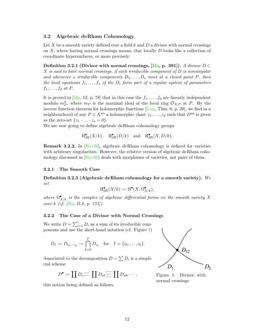
Figure 1: Divisor withnormal crossings

We write D =∑r

i=1Di as a sum of its irreducible com-ponents and use the short-hand notation (cf. Figure 1)

DI := Di0 ··· ip :=p⋂

k=0

Dik for I = i0, . . . , ik.

Associated to the decomposition D =∑Di is a simpli-

cial scheme

D• :=∐

Da←−←−∐

Dab←−←−←−

∐Dabc · · · ,

this notion being defined as follows.

12

Simplicial sets and simplicial schemes. We consider a category Simplex withobjects [m] := 0, . . . ,m, m ∈ N0, and <-order-preserving maps as morphisms.(Thus the existence of a map f : [m]→ [n] implies m ≤ n.)This category can be thought of as the prototype of a simplicial complex: Let K bea simplicial complex and assign to [m] the set of m-simplices of K. Any morphismf : [m]→ [n] maps each n-simplex to its m-dimensional “f -face”

f∗(e0, . . . , en) = (ef(0), . . . , ef(m)).

Thus K can be described by a contravariant functor to the category Sets of sets

Simplex −→ Sets.

A contravariant functor from Simplex to the category of sets, schemes, . . . is calleda simplicial set, simplicial scheme and so forth [GM, Ch. 1, 2.2, p. 9]. (There, as aslight generalization, the maps f : [m] → [n] are only required to be non-decreasinginstead of being <-order-preserving, thus allowing for “degenerate simplices”.)

In the above situation we define a simplicial scheme D• : Simplex→ Schemes by theassignment

[m] 7→∐

1≤i0<···<im≤rDi0 ··· im

(f : [m]→ [n]) 7→(D•(f) :

∐Di0 ··· in →

∐Di0 ··· im

);

here D•(f) is the sum of the natural inclusions

Di0 ··· in → Dif(0) ··· if(m).

If δml : [m]→ [m+ 1] denotes the unique <-order-preserving map, whose image doesnot contain l, we can represent D• by a diagram

r∐a=1

Da

D•(δ00)←−−−−D•(δ01)←−−−−

∐1≤a<b≤r

Dab

D•(δ10)←−−−−D•(δ11)←−−−−D•(δ12)←−−−−

∐1≤a<b<c≤r

Dabc · · · . (D•)

Now the differentials come into play again. We consider the contravariant functori∗Ω•?/k defined for subschemes Z of Supp(D)

i∗Ω•?/k : Z 7→ i∗Ω•Z/k.

where i stands for the natural inclusion Zi→ Supp(D). We enlarge the scope of

i∗Ω•?/k to schemes of the form∐a Za, Za ⊆ D by making the convention

(i∗Ω•?/k

)(∐a

Za

):=⊕a

i∗Ω•Za/k.

Composing D• with the contravariant functor i∗Ω•?/k yields a diagram

r⊕a=1

i∗Ω•Da/k

d00−−−−→d01−−−−→

⊕1≤a<b≤r

i∗Ω•Dab/k

d10−−−−→d11−−−−→d12−−−−→

⊕1≤a<b<c≤r

i∗Ω•Dabc/k· · · ,

13

where we have written dml for (i∗Ω•?/k D•)(δml ). Summing up these maps dml with

alternating signs

dm :=m∑l=0

(−1)ldml

gives a new diagram

r⊕a=1

i∗Ω•Da/kd0−−−−→

⊕1≤a<b≤r

i∗Ω•Dab/kd1−−−−→

⊕1≤a<b<c≤r

i∗Ω•Dabc/k· · · ,

which turns out to be a double complex (cf. the appendix) as a little calculationshows

dm+1 dm =m+1∑l=0

m∑k=0

(−1)l+k dm+1l dmk

=∑

0≤k<l≤m+1

(−1)l+k dm+1l dmk +

∑0≤l≤k≤m

(−1)l+k dm+1l dmk︸ ︷︷ ︸

=∑

0≤l≤k≤m(−1)l+k dm+1

k+1 dml

=∑

0≤k′<l′≤m+1

(−1)k′+l′−1 dm+1

l′ dmk′

=0.

We denote this double complex by Ω•,•D•/k and its total complex (cf. the appendix) by

Ω•D/k := tot Ω•,•D•/k.

Definition 3.2.4 (Algebraic deRham cohomology for a divisor). If D is adivisor with normal crossings on a smooth variety X over k, we define its algebraicdeRham cohomology by

H•dR(D/k) := H•(D; Ω•D/k).

Remark 3.2.5. Actually, we do not need that D ⊆ X has codimension 1 for thisdefinition; but D having normal crossings is essential.

3.2.3 The Relative Case

The natural restriction maps

Ω•X/k → (Di → X)∗Ω•Di/k

sum up to a natural map of double complexes

Ω•X/k[0]→ (Supp(D) → X)∗Ω•,•D•/k, (9)

14

where we view Ω•X/k[0] as a double complex concentrated in the zeroth column. Some-what sloppy, we will often write i∗F instead of (Supp(D) → X)∗F . Taking the totalcomplex in (9) yields a natural map

f : Ω•X/k → i∗Ω•D/k,

for whose mapping cone (cf. the appendix)

Mf = i∗Ω•D/k[−1]⊕ Ω•X/k with differential(−dD f

0 dX

)we write Ω•X,D/k.

Definition 3.2.6 (Relative algebraic deRham cohomology). For X a smoothvariety over k and D a divisor with normal crossings on X, we define the relativealgebraic deRham cohomology of the pair (X,D) by

H•dR(X,D/k) := H•(X; Ω•X,D/k).

These definitions may seem a bit technical at first glance. However, they will hopefullybecome more transparent in the sequel, when the existence of a long exact sequencein algebraic deRham cohomology and various comparison isomorphisms are proved.

3.3 Basic Lemmas

In this subsection we gather two basic lemmas for the ease of reference.

Lemma 3.3.1. If i : Z → X is a closed immersion and I an injective sheaf of abeliangroups on Z, then i∗I is also injective.

Proof. Let A B be an injective morphism of sheaves of abelian groups on X. Sincei−1 is an exact functor, the induced map

i−1A i−1B

will be injective as well. Now the adjoint property of i−1 provides us with the followingcommutative square

HomX(B, i∗I) ∼= HomZ(i−1B, I)↓ ↓

HomX(A, i∗I) ∼= HomZ(i−1A, I).

Because I is injective, the map on the right-hand-side is surjective. Hence so isthe left-hand map, which in turn implies the injectivity of i∗I, since A and B werearbitrary.

Lemma 3.3.2. If i : Z → X is a closed immersion and F• a complex of sheaves onZ, which is bounded below, then there is a natural isomorphism

H•(X; i∗F•) ∼= H•(Z;F•).

15

Proof. The point is that i∗ is an exact functor for closed immersions, which can beeasily checked on the stalks. Thus if F• I• is a quasi-isomorphism between F•and a complex I• consisting of injective sheaves, the induced map

i∗F• i∗I•

will be a quasi-isomorphism as well. But the sheaves i∗Ip are injective by Lemma3.3.1, hence we can use i∗I• to compute the hypercohomology of i∗F•

H•(X; i∗F•) = h•Γ(X; i∗I•).

Now the claim follows from the identity of functors Γ(X, i∗?) = Γ(Z; ?)

H•(X; i∗F•) = h•Γ(X; i∗I•) = h•Γ(Z; I•) = H•(Z;F•).

3.4 The Long Exact Sequence in Algebraic deRham Cohomology

Proposition 3.4.1. We have a natural long exact sequence in algebraic deRhamcohomology (as defined in Definition 3.2.3, 3.2.4 and 3.2.6)

· · · → Hp−1dR (D/k)→

HpdR(X,D/k)→ Hp

dR(X/k)→ HpdR(D/k)→

Hp+1dR (X,D/k)→ · · · ,

where X is a smooth variety over k and D a normal-crossings-divisor on X.

Proof. The short exact sequence of the mapping cone

0→ i∗Ω•D/k[−1]→ Ω•X,D/k → Ω•X/k → 0

gives us a long exact sequence in hypercohomology

· · · → Hp(X; i∗Ω•D/k[−1])→

Hp(X; Ω•X,D/k)→ Hp(X; Ω•X/k)→ Hp+1(X; i∗Ω•D/k[−1])→

Hp+1(X; Ω•X,D/k)→ · · · ,

which we can rewrite as

· · · → Hp−1(X; i∗Ω•D/k)→

HpdR(X,D/k)→ Hp

dR(X/k)→ Hp(X; i∗Ω•D/k)→

Hp+1dR (X,D/k)→ · · · .

By Lemma 3.3.2, we see

H•(X; i∗Ω•D/k) = H•(D; Ω•D/k) = H•dR(D/k)

and our assertion follows.

16

3.5 Behaviour Under Base Change

Let X0 be a smooth variety defined over a field k0 and D0 a divisor with normalcrossings on X0. For the base change to an extension field k of k0 we write

X := X0 ×k0 k and D := D0 ×k0 k.

Then we have the following proposition.

Proposition 3.5.1. In the above situation, there are natural isomorphisms betweenalgebraic deRham cohomology groups (as defined in definitions 3.2.3, 3.2.4, 3.2.6)

H•dR(X/k) ∼= H•dR(X0/k0)⊗k0 k,H•dR(D/k) ∼= H•dR(D0/k0)⊗k0 k and

H•dR(X,D/k) ∼= H•dR(X0, D0/k0)⊗k0 k.

Proof. Denote by π : X → X0 the natural projection. By [Ha, Prop. II.8.10, p. 175],we have

Ω•X/k = π∗Ω•X0/k0.

Now the natural mapπ−1Ω•X0/k0

→ π∗Ω•X0/k0

factors throughπ−1Ω•X0/k0

→ π−1Ω•X0/k0⊗k0 k

yielding a natural map

π−1Ω•X0/k0⊗k0 k → π∗Ω•X0/k0

= Ω•X/k,

which provides us with a morphism of spectral sequences

hp Hq(X;π−1Ω•X0/k0⊗k0 k) ⇒ Hn(X;π−1Ω•X0/k0

⊗k0 k)↓ ↓

hp Hq(X;π∗Ω•X0/k0) ⇒ Hn(X;π∗Ω•X0/k0

) .

We can rewrite the first initial term using the exactness of the functor ?⊗k0 k

Hq(X;π−1ΩpX0/k0

⊗k0 k) = Hq(X;π−1ΩpX0/k0

)⊗k0 k

= Hq(X0; ΩpX0/k0

)⊗k0 k.

Since “cohomology commutes with flat base extension for quasi-coherent sheaves” [Ha,Prop. III.9.3, p. 255], the map

Hq(X0; ΩpX0/k0

)⊗k0 k −→ Hq(X;π∗ΩpX0/k0

)

is an isomorphism. Hence we also have an isomorphism on the limit terms, for whichwe obtain

Hn(X;π−1Ω•X0/k0⊗k0 k) = Hn(X;π−1Ω•X0/k0

)⊗k0 k

= Hn(X0; Ω•X0/k0)⊗k0 k

= HndR(X0/k0)⊗k0 k

17

and

Hn(X;π∗Ω•X0/k0) = Hn(X; Ω•X/k)

= HndR(X/k).

The other two statements can be proved analogously. (Observe that the sheavesΩpD0/k0

and ΩpX0,D0/k0

are quasi-coherent by [Ha, Prop. II.5.8(c), p. 115].)

3.6 Some Spectral Sequences

Before we proceed in the discussion of algebraic deRham cohomology, we have tomake a digression and provide some spectral sequences which we will need later on.

3.6.1 Cech Cohomology

We adopt the notation from [Ha, III.4]: Let X be a topological space, U = (Uj)j∈Jan open covering of X and F a sheaf of abelian groups on X. We assume J to bewell-ordered. As usual, we use the short-hand notation

UI := Ui0 ··· im :=m⋂k=0

Uik for I = i0, . . . , im.

Recall that in this situation we have a Cech functor defined on the category Ab(X)of sheaves of abelian groups on X (cf. [Ha, III.4, p. 220])

Cp(U, ?) : Ab(X)→ Ab(X)

F 7→⊕|I|=p+1I⊆J

i∗F|UI,

where i stands for the respective inclusions UI → X, and a differential

d : Cp(U;F)→ Cp+1(U;F),

which makes C•(U,F) into a complex. We explain this d below. We also need Cechgroups

Cp(U;F) := Γ(X; Cp(U;F))

and of course Cech cohomology

Hp(U;F) := hp C•(U;F).

Clearly, we can consider the Cech functor also for closed coverings; but then Cechcohomology will not behave particularly well.

We can give the following fancy definition of the Cech complex C•(U;F). The assign-ment

U• : Simplex→ Schemes

[m] 7→∐

i0<···<im

Ui0 ··· im

(f : [m]→ [n]) 7→(U•(f) :

∐Ui0 ··· in →

∐Ui0 ··· im

)18

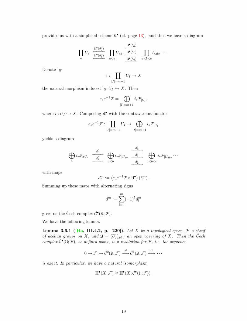
provides us with a simplicial scheme U• (cf. page 13), and thus we have a diagram

∐a

UaU•(δ00)←−−−−U•(δ01)←−−−−

∐a<b

Uab

U•(δ10)←−−−−U•(δ11)←−−−−U•(δ12)←−−−−

∐a<b<c

Uabc · · · .

Denote byε :

∐|I|=m+1

UI → X

the natural morphism induced by UI → X. Then

ε∗ε−1F =

⊕|I|=m+1

i∗F|UI,

where i : UI → X. Composing U• with the contravariant functor

ε∗ε−1F :

∐|I|=m+1

UI 7→⊕

|I|=m+1

i∗F|UI

yields a diagram

⊕a

i∗FxUa

d00−−−−→d01−−−−→

⊕a<b

i∗F|Uab

d10−−−−→d11−−−−→d12−−−−→

⊕a<b<c

i∗F|Uabc· · ·

with mapsdml :=

(ε∗ε−1F U•

)(δml ).

Summing up these maps with alternating signs

dm :=m∑l=0

(−1)l dml

gives us the Cech complex C•(U;F).

We have the following lemma.

Lemma 3.6.1 ([Ha, III.4.2, p. 220]). Let X be a topological space, F a sheafof abelian groups on X, and U = (Uj)j∈J an open covering of X. Then the Cechcomplex C•(U;F), as defined above, is a resolution for F , i.e. the sequence

0→ F C0(U;F) d0−→ C1(U;F) d1−→ · · ·

is exact. In particular, we have a natural isomorphism

H•(X;F) ∼= H•(X; C•(U;F)).

19

3.6.2 A Spectral Sequence for Hypercohomology of an Open Covering

We generalize the well-known spectral sequence of an open covering U of a space X(where Hq(F) is the presheaf V 7→ Hq(V ;F|V ))

Hp(U;Hq(F))⇒ Hn(X;F)

to the case of a complex F• of abelian sheaves and its hypercohomology.Let X be a topological space, U = (Uj)j∈J an open covering of X and F• a complexof sheaves of abelian groups on X, which is bounded below. We define a presheaf

Hp(F•) : V 7→ Hp(V ;F•|V ) for V ⊆ X open

as a “sheafified” version of hypercohomology.

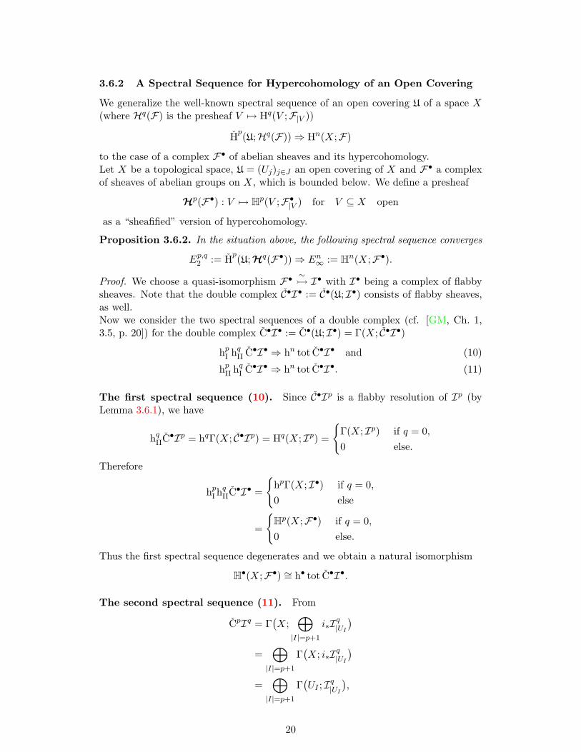
Proposition 3.6.2. In the situation above, the following spectral sequence converges

Ep,q2 := Hp(U;Hq(F•))⇒ En∞ := Hn(X;F•).

Proof. We choose a quasi-isomorphism F•∼ I• with I• being a complex of flabby

sheaves. Note that the double complex C•I• := C•(U; I•) consists of flabby sheaves,as well.Now we consider the two spectral sequences of a double complex (cf. [GM, Ch. 1,3.5, p. 20]) for the double complex C•I• := C•(U; I•) = Γ(X; C•I•)

hpI hqII C•I• ⇒ hn tot C•I• and (10)

hpII hqI C•I• ⇒ hn tot C•I•. (11)

The first spectral sequence (10). Since C•Ip is a flabby resolution of Ip (byLemma 3.6.1), we have

hqIIC•Ip = hqΓ(X; C•Ip) = Hq(X; Ip) =

Γ(X; Ip) if q = 0,0 else.

Therefore

hpI hqIIC•I• =

hpΓ(X; I•) if q = 0,0 else

=

Hp(X;F•) if q = 0,0 else.

Thus the first spectral sequence degenerates and we obtain a natural isomorphism

H•(X;F•) ∼= h• tot C•I•.

The second spectral sequence (11). From

CpIq = Γ(X;

⊕|I|=p+1

i∗Iq|UI

)=

⊕|I|=p+1

Γ(X; i∗Iq|UI

)=

⊕|I|=p+1

Γ(UI ; Iq|UI

),

20

we see

hqI CpI• =

⊕|I|=p+1

hqΓ(UI ; I•|UI

)=

⊕|I|=p+1

Hq(UI ;F•|UI

)=

⊕|I|=p+1

Γ(UI ;Hq(F•)|UI

)=

⊕|I|=p+1

Γ(X; i∗Hq(F•)|UI

)= Γ

(X;

⊕|I|=p+1

i∗Hq(F•)|UI

)= Γ

(X; Cp

(U;Hq(F•)

))= Cp

(U;Hq(F•)

).

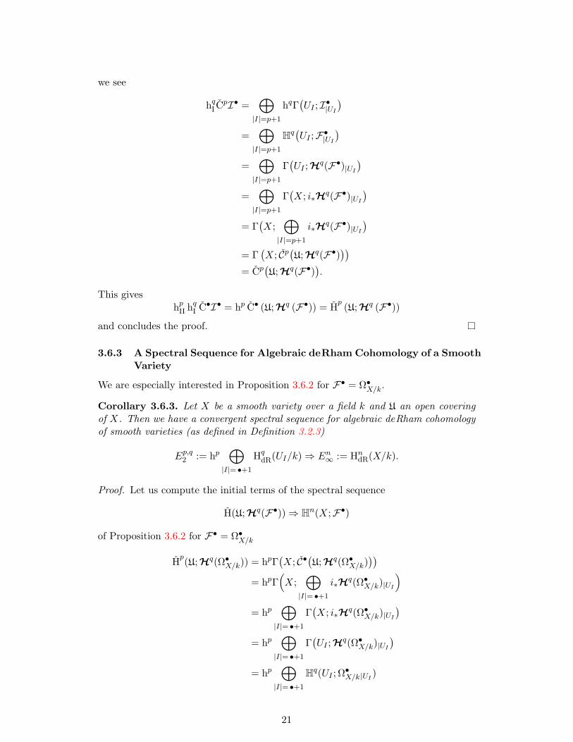
This giveshpII hqI C•I• = hp C• (U;Hq (F•)) = Hp (U;Hq (F•))

and concludes the proof.

3.6.3 A Spectral Sequence for Algebraic deRham Cohomology of a SmoothVariety

We are especially interested in Proposition 3.6.2 for F• = Ω•X/k.

Corollary 3.6.3. Let X be a smooth variety over a field k and U an open coveringof X. Then we have a convergent spectral sequence for algebraic deRham cohomologyof smooth varieties (as defined in Definition 3.2.3)

Ep,q2 := hp⊕|I|= •+1

HqdR(UI/k)⇒ En∞ := Hn

dR(X/k).

Proof. Let us compute the initial terms of the spectral sequence

H(U;Hq(F•))⇒ Hn(X;F•)

of Proposition 3.6.2 for F• = Ω•X/k

Hp(U;Hq(Ω•X/k)) = hpΓ(X; C•

(U;Hq(Ω•X/k)

))= hpΓ

(X;

⊕|I|= •+1

i∗Hq(Ω•X/k)|UI

)= hp

⊕|I|= •+1

Γ(X; i∗Hq(Ω•X/k)|UI

)= hp

⊕|I|= •+1

Γ(UI ;Hq(Ω•X/k)|UI

)= hp

⊕|I|= •+1

Hq(UI ; Ω•X/k |UI)

21

= hp⊕|I|= •+1

Hq(UI ; Ω•UI/k)

= hp⊕|I|= •+1

HqdR(UI/k).

For the limit term we get immediately

H•(X; Ω•X/k) = H•dR(X/k)

and the corollary is proved.

3.6.4 A Spectral Sequence for Algebraic deRham Cohomology of a Divi-sor with Normal Crossings

For a divisorD with normal crossings, we have a spectral sequence expressing H•dR(D/k)in terms of H•dR(Di0 ··· im/k).Recall that (cf. page 14)

Ω•D/k = tot Ω•,•D•/k = tot⊕|I|

i∗Ω•DI/k.

Since we are interested in hypercohomology, we replace the Ω•∗ by their Godementresolutions (cf. page 8), where we shall use the following abbreviations

• GpDI/k:= GpΩ•

DI/k,

• Gp,qD•/k := GpΩ•,q

D/k

=⊕|I|=q+1 G

pi∗Ω•

DI/k

(∗)=⊕|I|=q+1 i∗G

pDI/k

,

(we have equality at (∗) since i∗ is exact for closed immersions i)

and

• G•D/k := G•eΩ•D/k

= G•totΩ•,•

D•/k

= totG•,•D•/k.

Furthermore, we write

GpDI/k

:= Γ(DI ;GpDI/k

), Gp,q

D•/k := Γ(D;Gp,qD•/k

)and Gp

D/k := Γ(D;GpD/k

)for the groups of global sections of these sheaves.We consider the second spectral sequence for the double complex Gp,q

D•/k

hpII hqI G•,•D•/k ⇒ hn totG•,•D•/k.

For the limit terms, we obtain

hn totG•,•D•/k = hnG•D/k = hnΓ(D;G•D/k) = Hn(D; Ω•D/k) = HndR(D/k).

22

Let us compute the initial terms

hqG•,pD•/k = hqΓ(D;⊕|I|=p+1

i∗G•DI/k)

= hq⊕|I|=p+1

Γ(D; i∗G•DI/k)

=⊕|I|=p+1

hqΓ(D; i∗G•DI/k)

=⊕|I|=p+1

hqΓ(DI ;G•DI/k)

=⊕|I|=p+1

Hq(DI ; Ω•DI/k)

=⊕|I|=p+1

HqdR(DI/k).

Thus we have proved the following proposition.

Proposition 3.6.4. Let X be a smooth variety over a field k and D a divisor withnormal crossings on X. Then we have a convergent spectral sequence for algebraic deRham cohomology of a divisor (as defined in Definition 3.2.4)

Ep,q2 := hp⊕|I|= •+1

HqdR(DI/k)⇒ En∞ := Hn

dR(D/k).

23

4 Comparison Isomorphisms

If we consider a smooth variety X defined over C and a divisor D with normalcrossings on X, then their algebraic deRham cohomology as defined in Subsection3.2 turns out to be naturally isomorphic to the singular cohomology of the associatedcomplex analytic spaces Xan and Dan.Our proof proceeds in three steps: (1) First we mimic the definition of algebraicdeRham cohomology in the complex analytic setting using holomorphic differentialforms instead of algebraic ones, thus defining analytic deRham cohomology groups

H•dR(Xan; C), H•dR(Dan; C) and H•dR(Xan, Dan; C).

These are then shown to be isomorphic to their algebraic counterparts using an ap-plication of Serre’s “GAGA-type” results by Grothendieck.(2) In the second step, analytic deRham cohomology is proved to coincide with com-plex cohomology, (3) which in turn is isomorphic to singular cohomology, as we showin the third step. (In the smooth case this has already been shown in Proposition3.1.2.)

4.1 Situation

Throughout this section, X will be a smooth variety over C and D a divisor withnormal crossings on X. As usual, we denote the complex analytic spaces associatedto X and D by Xan and Dan, respectively (cf. Definition 2.1.3).

4.2 Analytic deRham Cohomology

If we replace in Subsection 3.2 every occurrence of the complex of algebraic differentialforms Ω•Y/C on a complex variety Y by the complex of holomorphic differential formsΩ•Y an on the associated complex analytic space Y an, we obtain complexes

Ω•Xan , Ω•,•Dan• , Ω•Dan and Ω•Xan,Dan

and thus are able to define:

Definition 4.2.1 (Analytic deRham cohomology). For Xan and Dan as in Sub-section 4.1, we define analytic deRham cohomology by

H•dR(Xan; C) := H•(Xan; Ω•Xan), (∗)

H•dR(Dan; C) := H•(Dan; Ω•Dan) and

H•dR(Xan, Dan; C) := H•(Xan; Ω•Xan,Dan).

Here (∗) is the definition of analytic deRham cohomology for complex manifolds al-ready considered on page 11, which we listed again for completeness.

Note that (Ω•Y/C)an = Ω•Y an , hence

(Ω•X/C)an = Ω•Xan ,

(Ω•,•D•/C)an = Ω•,•Dan• ,

(Ω•D/C)an = Ω•Dan and

(Ω•X,D/C)an = Ω•Xan,Dan .

(12)

24

Remark 4.2.2. We could easily generalize Definition 4.2.1 to arbitrary complex ma-nifolds (and normal-crossings-divisors on them) not necessarily associated to some-thing algebraic, but we will not need this.

4.3 The Long Exact Sequence in Analytic deRham Cohomology

The results of Subsection 3.4 carry over one-to-one to the complex analytic case.

Proposition 4.3.1. We have naturally a long exact sequence in analytic deRhamcohomology (as defined in Definition 4.2.1)

· · · → Hp−1dR (Dan; C)→

HpdR(Xan, Dan; C)→ Hp

dR(Xan; C)→ HpdR(Dan; C)→

Hp+1dR (Xan, Dan; C)→ · · · ,

where Xan and Dan are as in Subsection 4.1.

Moreover, by Equation (8) on page 9 and Equation (12), we have a natural morphismfrom the long exact sequence in algebraic deRham cohomology to the one in analyticdeRham cohomology

· · · → HpdR(X,D/C) −−−−→ Hp

dR(X/C) −−−−→ HpdR(D/C) → · · ·y y y

· · · →HpdR(Xan, Dan; C) −−−−→ Hp

dR(Xan; C) −−−−→ HpdR(Dan; C)→ · · · .

(13)

We want to show that all the vertical maps are isomorphisms.

4.4 Some Spectral Sequences for Analytic deRham Cohomology

The proof of Proposition 3.6.3 applies in the analytic case as well and we obtain

Proposition 4.4.1. We have a convergent spectral sequence for analytic deRhamcohomology (as defined in Definition 4.2.1)

Ep,q2 := hp⊕|I|= •+1

HqdR(Uan

I ; C)⇒ En∞ := HndR(Xan; C),

where Xan is associated to a smooth variety X over C and U = (Uj)j∈J is an opencovering of X.

Furthermore, the natural map of hypercohomology groups (cf. (8) and (12))

H•(U ; Ω•U/C)→ H•(Uan; Ω•Uan) for U ⊆ X open,

provides us with a natural map of spectral sequences

Hp(U;Hq(Ω•X/C))⇒ Hn(X; Ω•X/C)

↓ ↓Hp(Uan;Hq(Ω•Xan))⇒ Hn(Xan; Ω•Xan),

25

which we can rewrite using Corollary 3.6.3 and Proposition 4.4.1

hp⊕|I|= •+1

HqdR(UI/C)⇒ Hn

dR(X/C)y yhp

⊕|I|= •+1

HqdR(Uan

I ; C)⇒ HndR(Xan; C).

(14)

Likewise, we can transfer Proposition 3.6.4 to the analytic case.

Proposition 4.4.2. We have a convergent spectral sequence

Ep,q2 := hp⊕|I|= •+1

HqdR(Dan

I ; C)⇒ En∞ := HndR(Dan; C),

where Dan is associated to a normal-crossings-divisor D on a smooth variety X definedover C as in Subsection 4.1.

Again, we have a natural map of spectral sequences. We write (cf. page 22)

Gp,qDan• :=(Gp,qD•/C

)an

andGp,qDan• := Γ(Dan;Gp,qDan•).

Now the natural map of zeroth homology (cf. Equation (3) for i = 0)

G•,•D•/C → G•,•Dan•

gives us a natural map of spectral sequences

hpI hqII G•,•D•/C ⇒ hn totG•,•D•/C

↓ ↓hpI hqII G•,•Dan• ⇒ hn totG•,•Dan• .

With propositions 3.6.4 and 4.4.2, this map takes the form

hp⊕|I|= •+1

HqdR(DI/C)⇒ Hn

dR(D/C)y yhp

⊕|I|= •+1

HqdR(Dan

I ; C)⇒ HndR(Dan; C).

(15)

4.5 Comparison of Algebraic and Analytic deRham Cohomology

The proof of H•dR(X/C) ∼= H•dR(Xan; C), i.e. H•(X; Ω•X/C) ∼= H•(Xan; Ω•Xan) is easyin the projective case, because of (12) and Corollary 2.2.4.The affine case is contained in a theorem of Grothendieck.

Theorem 4.5.1 (Grothendieck, [Gro, Thm. 1, p. 95]). Let X be a smoothaffine variety over C. Then the natural map between algebraic and analytic deRhamcohomology (as defined in definitions 3.2.3 and 4.2.1)

H•dR(X/C) ∼−→ H•dR(Xan; C)

is an isomorphism.

26

We give only some comments on the proof. Let j : X → X be the projective closureof X and let Z := X \X. Furthermore, we set

Ω•X/C(∗Z) := lim−→

n

Ω•X/C(nZ) and

Ω•X

an(∗Zan) := lim−→n

Ω•X

an(nZan),

where F(nZ ′) denotes the sheaf F twisted by the n-fold of the divisor Z ′. In hispaper [Gro], Grothendieck considers the following chain of isomorphisms:

H•dR(X/C) = H•(X; Ω•X/C)xo ΩpX/C are Γ(X; ?)-acyclic [Ha, Thm. III.3.5, p. 215]

h•Γ(X; Ω•X/C)‖

h•Γ(X; j∗Ω•X/C)‖

h•Γ(X; Ω•X/C(∗Z))yo [Ha, Prop. III.2.9, p. 209]

lim−→n

h•Γ(X; Ω•X/C(nZ))yo Thm. 2.2.3 (GAGA)

lim−→n

h•Γ(Xan; Ω•X

an(nZan))yo [AH, Lemma 6]

h•Γ(Xan; Ω•X

an(∗Zan))yo main step

h•Γ(Xan; j∗Ω•Xan)‖

h•Γ(Xan; Ω•Xan)yo ΩpXan are Γ(Xan; ?)-acyclic since Xan is Stein

[GR, IV.1.1, Def. 1, p. 103; V.1, Bem., p. 130]H•dR(Xan; C) = H•(Xan; Ω•Xan).

In the case that Z has normal crossings, the main step is due to Atiyah and Hodge[AH, Lemma 17] and is proved by explicit calculations. Grothendieck reduces thegeneral case to this one by using the resolution of singularities according to Hironaka[Hi1].

The smooth case. Choose an open affine covering U = (Uj)j∈J of X. Since X isseparated, all the UI are affine. Hence by Theorem 4.5.1 we get an isomorphism onthe initial terms in (14), and therefore also on the limit terms

H•dR(X/C) ∼= H•dR(Xan; C).

27

The case of a normal-crossings-divisor. Since D is a divisor with normal cross-ings, all the DI are smooth. Thus we see from the discussion of the smooth case, thatwe have an isomorphism on the initial terms in (15), hence also on the limit terms

H•dR(D/C) ∼= H•dR(Dan; C).

The relative case. By the 5-lemma, this case follows immediately from the twocases considered above using diagram (13).

We summarize our results so far.

Proposition 4.5.2. For X a smooth variety over C and D a normal-crossings-divisoron X, we have a natural isomorphism between algebraic deRham cohomology of Xand D (see definitions 3.2.3, 3.2.4, 3.2.6) and analytic deRham cohomology (seeDefinition 4.2.1) of the associated complex analytic spaces Xan and Dan

· · · → HpdR(X,D/C) −−−−→ Hp

dR(X/C) −−−−→ HpdR(D/C) → · · ·yo yo yo

· · · →HpdR(Xan, Dan; C) −−−−→ Hp

dR(Xan; C) −−−−→ HpdR(Dan; C)→ · · · .

4.6 Complex Cohomology

Definition 4.6.1 (Complex cohomology). Let Xan and Dan be as in Subsection4.1. In the absolute case, complex cohomology is simply sheaf cohomology of theconstant sheaf with fibre C

H•(Xan; C) := H•(Xan; CXan) and H•(Dan; C) := H•(Dan; CDan).

We define a relative version by

H•(Xan, Dan; C) := H•(Xan; j!CUan),

where U := X \D and j : U → X.

Remark 4.6.2. Taking Q instead of C in the above definition would give us rationalcohomology groups H•(Xan; Q), H•(Dan; Q) and H•(Xan, Dan; Q).

The short exact sequence

0→ j!CUanα−→ CXan → i∗CDan → 0 (16)

with j : Uan → Xan and i : Dan → Xan, yields a long exact sequence in complexcohomology

· · · → Hp−1(Dan; C)→Hp(Xan, Dan; C)→ Hp(Xan; C)→ Hp(Dan; C)→Hp+1(Xan, Dan; C)→ · · · .

The mapping cone MC (cf. the appendix) of the natural restriction map CXan →i∗CDan gives us another short exact sequence

0→ i∗CDan [−1]→MC → CXan [0]→ 0. (17)

28

Consider the map

γ := (0, α) : j!CUan [0]→MC = i∗CDan [−1]⊕ CXan [0],

where α : j!CUan [0] → CXan [0] was defined in (16) and 0 : j!CUan → i∗CDan [−1]denotes the zero map. In order to show that α is a morphism of complexes, we onlyhave to check the compatibility of the differentials, but this follows from the fact that(16) is a complex. The exactness of the sequence in (16) translates into γ being aquasi-isomorphism. This gives us the following diagram

Hp−1(Dan; C) →Hp(Xan, Dan; C)→ Hp(Xan; C) → Hp(Dan; C)‖ ‖ ‖ ‖

Hp(Xan; i∗CDan [−1])→ Hp(Xan;MC) →Hp(Xan; CXan [0])→Hp+1(Xan; i∗CDan [−1]).

Unfortunately, this diagram does not commute (there is a sign mismatch), so weconsider the natural transformation

εp = (−1)p id for p ∈ Z

and write down a new diagram

Hp−1(Dan; C) →Hp(Xan, Dan; C)→ Hp(Xan; C) → Hp(Dan; C)εp−1 ↓ o εp ↓ o εp ↓ o εp ↓ o

Hp(Xan; i∗CDan [−1])→ Hp(Xan;MC) →Hp(Xan; CXan [0])→Hp+1(Xan; i∗CDan [−1]) .

This diagram commutes as we see by replacing the sheaves involved in (16) by injectiveresolutions A•, B• and C• and applying Lemma 4.6.3 below to the complexes A•, B•

and C• of their global sections.

Lemma 4.6.3. Let0 −→ A• α−→ B•

β−→ C• −→ 0

be a short exact sequence of complexes of abelian groups and

0 −→ C•[−1] ι−→ M• π−→ B• −→ 0

the mapping cone of β : B• → C•. Then we have a quasi-isomorphism

γ := (0, α) : A• ∼−→ M• = C•[−1]⊕ B•

and a commutative diagram

hp−1C• δ−−−−→ hpA• α∗−−−−→ hpB•β∗−−−−→ hpC•

εp−1

yo 1 εpγ∗yo εp

yo 2 εp

yohp−1C• ι∗−−−−→ hpM• π∗−−−−→ hpB• δ′−−−−→ hpC• .

Proof. The assertion about the quasi-isomorphism γ : A• → M• follows from theexactness of 0 → A• → B• → C• → 0. The middle square commutes because ofπ γ = α. So we are left to show the commutativity of the squares 1 and 2 .

29

Ad 2 .) From the diagram

Cp ι−→ Mp+1

↑ dMMp π−→ Bp

and the definition of the connecting morphism δ′ we see for b ∈ Bp

δ′[b] = [β(b)] = β∗[b],

hence(δ′ εp)[b] = (εp β∗)[b].

Ad 1 .) Pick an element c ∈ Cp−1 and choose a preimage b ∈ Bp−1. With

Ap α−→ Bp

↑ dBBp−1 β−→ Cp−1

we getδ[c] = [α−1 dBb] ∈ hpA•.

Applying γ∗ gives

(γ∗ δ)[c] = (0, α)∗[α−1 dBb] = [0, dBb] ∈ hpM• = hp(C•[−1]⊕ B•)

or after subtracting the coboundary dM(0, b) = (β(b), dBb) = (c, dBb)

(γ∗ δ)[c] = [−c, 0] = −ι∗[c],

hence(εp γ∗ δ)[c] = (ι∗ εp−1)[c].

4.7 Comparison of Analytic deRham Cohomology and Complex Co-homology

We apply the Cech functor (cf. Subsection 3.6.1) for the closed covering D :=(Dan

i )ri=1 to the constant sheaf CDan , and thus get Cq(D; C) := Cq(D; CDan). Nowthe natural inclusions CDan

I→ Ω0

DanI

sum up to a natural morphism of sheaves onDan

Cq(D; C) =⊕|I|=q+1

i∗CDanI

↓

Ω0,qDan• =

⊕|I|=q+1

i∗Ω0Dan

I,

(18)

where i : DanI → Dan. Since the complexes Ω•Dan

Iare resolutions of the sheaves CDan

I

and i∗ and ⊕ are exact functors, this shows that Ω•,qDan• is a resolution of Cq(D; C).

30

If we consider C•(D; C)[0] as a double complex (cf. the appendix) concentrated inthe zeroth row, we can rewrite (18) as

C•(D; C)[0]→ Ω•,•Dan•

or, after taking the total complex, as

C•(D; C)→ Ω•Dan .

This morphism is a quasi-isomorphism by Lemma 2.2.5 (and Remark 2.2.6) and fitsinto the following commutative diagram

CXan [0] → i∗CDan [0]‖ ↓ α

CXan [0] → i∗C•(D; C)↓ o ↓ o

Ω•Xan → i∗Ω•Dan .

The map α is a quasi-isomorphism as a consequence of the following proposition.

Proposition 4.7.1. We have an exact sequence

0→ CDan → C0(D; C)→ C1(D; C)→ · · · .

Proof (cf. [Ha, Lemma III.4.2, p. 220]). This can be checked on the stalks and istherefore a purely combinatorial problem. Let x ∈ Dan and assume w.l.o.g. thatthe irreducible components Dan

1 , . . . , Dans but no other component of Dan are passing

through x. For the stalks at x, we write

Cp := Cp(D; C)x =⊕

1≤i0<···<ip≤sCDan

i0 ··· ip,x.

Observe that exactness at the zeroth and first step is obvious. Using the “coordinatefunctions” for a set of indices j0, . . . , jp

Cp =⊕

1≤i0<···<ip≤sCDan

i0 ··· ip,x CDan

j0 ··· jp,x

⊕αi0 ··· ip 7→ αj0 ··· jp

we define a homotopy operator

kp : Cp → Cp−1

such that for any α ∈ Cp the “coordinates” of its image kp(α) satisfy

kp(α)j0 ··· jp−1 =

0 if j0 = 1α1 j0 ··· jp−1 else.

Now an elementary calculation shows that for p ≥ 1

dp−1 kp + kp+1 dp = idCp .

Hence k is a homotopy between the identity map and the zero map on C•, and weconclude that

hp C• = 0 for p ≥ 1.

31

Thus we have a commutative diagram

CXan [0] −−−−→ i∗CDan [0]yo yoΩ•Xan −−−−→ i∗Ω•Dan ,

where the vertical maps are quasi-isomorphisms. As a consequence, we also have aquasi-isomorphism between the respective mapping cones

0 −−−−→ i∗CDan [−1] −−−−→ MC −−−−→ CXan [0] −−−−→ 0yo yo yo0 −−−−→ i∗Ω•Dan [−1] −−−−→ Ω•Xan,Dan −−−−→ Ω•Xan −−−−→ 0 .

(19)

Taking hypercohomology proves the following proposition.

Proposition 4.7.2. We have a natural isomorphism between the long exact sequencein analytic deRham cohomology (cf. Definition 4.2.1) and the sequence in complexcohomology (cf. Definition 4.6.1)

· · · →Hp−1dR (Xan; C) −−−−→ Hp−1

dR (Dan; C) −−−−→ HpdR(Xan, Dan; C) → · · ·xo xo xo

· · · →Hp−1(Xan; C) −−−−→ Hp−1(Dan; C) −−−−→ Hp(Xan, Dan; C) → · · · ,

where Xan and Dan are as usual (see Subsection 4.1).

4.8 Singular Cohomology

We extend the definition of singular cohomology given on page 11

H•sing(Xan; C) := h•Γ

(Xan; C•sing(X

an; C))

and

H•sing(Dan; C) := h•Γ

(Dan; C•sing(D

an; C))

by a relative version.

Definition 4.8.1 (Relative singular cohomology). As usual, let Xan and Dan beas in Subsection 4.1. We set

C•sing(Xan, Dan; C) := ker(C•sing(X

an; C)→ i∗C•sing(Dan; C))

and defineH•sing(X

an, Dan; C) := h•Γ(Xan; C•sing(Xan, Dan; C)).

Remark 4.8.2. Similarly, one defines singular cohomology H•sing(Xan, Dan; k) with

coefficients in a field k different from C. We will need H•sing(Xan, Dan; Q) occasionly.

Since ?⊗Q C is an exact functor, we have

H•sing(Xan, Dan; Q)⊗Q C = H•sing(X

an, Dan; C).

32

The sheaf C•sing(Xan, Dan; C) is Γ(Xan; ?)-acyclic because of the surjectivity of

C•sing(Xan; C) C•sing(D

an; C) = Γ(Xan; i∗C•sing(Dan; C)).

Thus the short exact sequence

0→ C•sing(Xan, Dan; C)→ C•sing(X

an; C)→ i∗C•sing(Dan; C)→ 0

gives rise to a long exact sequence in singular cohomology

· · · → Hp−1sing(D

an; C)→Hp

sing(Xan, Dan; C)→ Hp

sing(Xan; C)→ Hp

sing(Dan; C)→

Hp+1sing(X

an, Dan; C)→ · · · .

4.9 Comparison of Complex Cohomology and Singular Cohomology

We have a commutative diagram

0 −−−−→ j!CUan [0] −−−−→ CXan [0] −−−−→ i∗CDan [0] −−−−→ 0yα yβ yγ0 −−−−→ C•sing(X

an, Dan; C) −−−−→ C•sing(Xan; C) −−−−→ i∗C•sing(D

an; C) −−−−→ 0,(20)

where β and γ are quasi-isomorphisms, since the singular cochain complex is a resolu-tion of the constant sheaf (see Proposition 3.1.1) and i∗ is exact for closed immersions.Therefore α is also a quasi-isomorphism.Taking hypercohomology gives a natural isomorphism between the long exact se-quence in complex cohomology and the sequence in singular cohomology. Thus wehave finally proved the following theorem.

4.10 Comparison Theorem

Theorem 4.10.1 (Comparison theorem). Let X be a smooth variety defined overC and D a divisor on X with normal crossings (cf. Definition 3.2.1). The associatedcomplex analytic spaces (cf. Subsection 2.1) are denoted by Xan and Dan, respectively.Then we have natural isomorphisms between the long exact sequences in

• algebraic deRham cohomology (cf. definitions 3.2.3, 3.2.4, 3.2.6),

• analytic deRham cohomology (cf. Definition 4.2.1),

• complex cohomology (cf. Definition 4.6.1), and

• singular cohomology (cf. Definition 4.8.1)

33

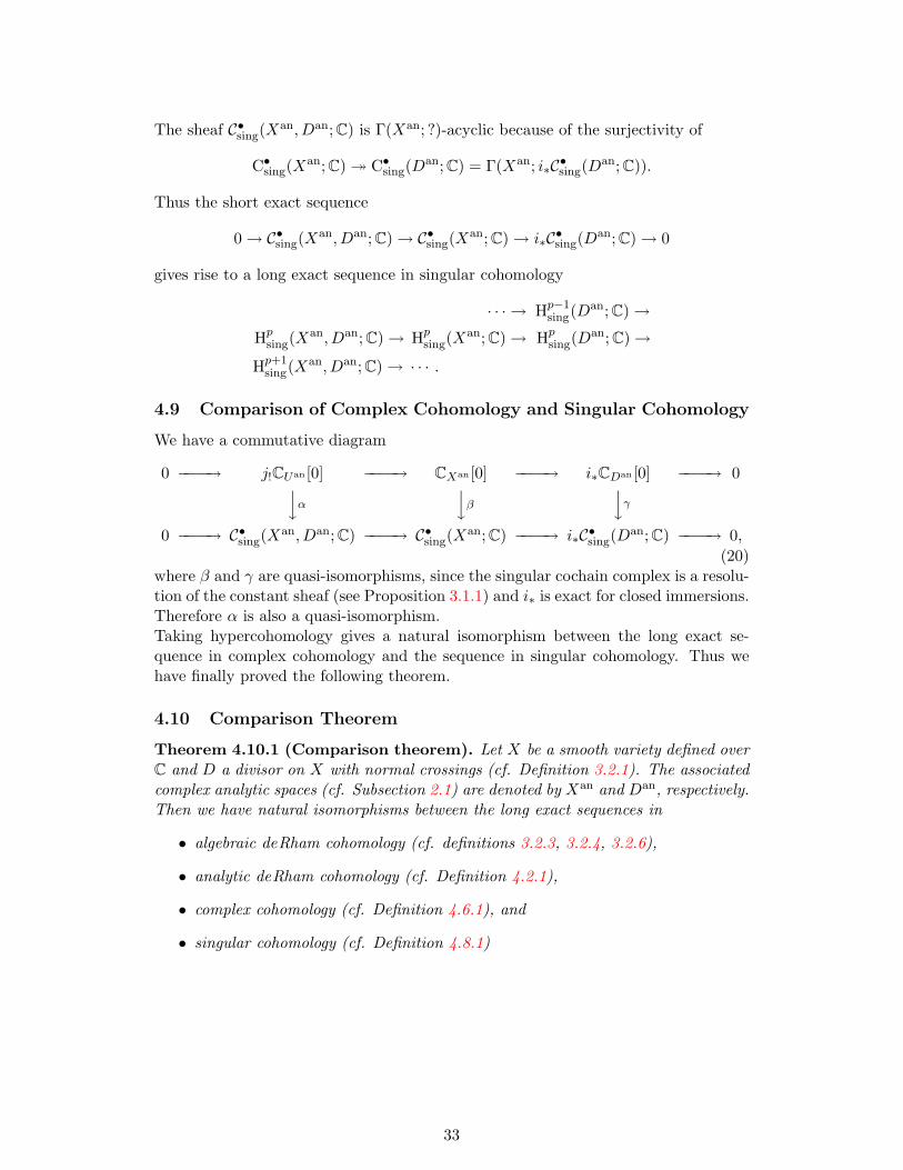
as shown in the commutative diagram below

· · · −→ HpdR(X,D/C) −−−−→ Hp

dR(X/C)algebraic deRham cohomology

−−−−→ HpdR(D/C) −→ · · ·yo yo yo

· · · −→ HpdR(Xan, Dan; C) −−−−→ Hp

dR(Xan; C)analytic deRham cohomology

−−−−→ HpdR(Dan; C) −→ · · ·xo xo xo

· · · −→ Hp(Xan, Dan; C) −−−−→ Hp(Xan; C)complex cohomology

−−−−→ Hp(Dan; C) −→ · · ·yo yo yo· · · −→Hp

sing(Xan, Dan; C) −−−−→ Hp

sing(Xan; C)

singular cohomology

−−−−→ Hpsing(D

an; C)−→ · · · .

Proof. Combine propositions 4.5.2 and 4.7.2 with the result from Subsection 4.9.

4.11 An Alternative Description of the Comparison Isomorphism

For computational purposes, it will be useful to describe the isomorphism from theComparison Theorem 4.10.1

H•dR(Xan; C) ∼= H•sing(Xan; C)

more explicitely. We will formulate our result in Proposition 4.11.5 and explain itssignificance in Subsection 4.11.5. We start by defining yet another cohomology theory.

4.11.1 Smooth Singular Cohomology

Let M be a complex manifold. We write 4stdp for the standard p-simplex spanned

by the basis (0, . . . , 0, 1i, 0, . . . , 0) | i = 1, . . . , p + 1 of Rp+1. A singular p-simplex

σ : 4stdp →M is said to be smooth, if σ extends to a smooth map defined on a neigh-

bourhood of the standard p-simplex 4stdp in its p-plane. We denote by C∞p (M ; C) the

C-vector space generated by all smooth p-simplices of M , thus getting a subcomplexC∞• (M ; C) of the complex Csing

• (M ; C) of all singular simplices on M

C∞• (M ; C) ⊂ Csing• (M ; C).

We can dualize this subcomplex

C•∞(M ; C) := C∞• (M ; C)∨,

and define a complex of sheaves

C•∞(M ; C) : V 7→ C•∞(V ; C) for V ⊆M open.

The sheaves Cp∞(M ; Q) are flabby and define smooth singular cohomology of M .

Definition 4.11.1 (Smooth singular cohomology of a manifold). Let M be acomplex manifold. We define smooth singular cohomology groups

H•∞(M ; C) := h•C•∞(M ; C) = H•(M ; C•∞(M ; C)

).

34

Since smooth singular cohomology coincides with singular cohomology for smoothmanifolds (cf. [Br, p. 291]), we can show that C•∞(M ; C) is a resolution of the constantsheaf CM exactly as we did for C•sing(M ; C) in Lemma 3.1.1. Thus we have thefollowing lemma.

Lemma 4.11.2. For M a complex manifold, the following sequence is exact

0 −→ CM −→ C0∞(M ; C) −→ C1

∞(M ; C) −→ . . . .

We are now going to extend the definition of smooth singular cohomology to the caseof a divisor and to the relative case. Let Xan and Dan be as in Subsection 4.1.First, recall how Ω•Dan was defined (cf. pages 14 and 24): We composed the simpli-cial scheme D• with the functor i∗Ω•?an , then obtained a double complex Ω•,•Dan• bysumming up certain maps and finally denoted the total complex of Ω•,•Dan• by Ω•Dan .Similarly, we can use the functor i∗C•∞(?an; C), compose it to the simplicial schemeD• and denote the resulting double complex by C•,•∞ (Dan; C). For the correspondingtotal complex we write C•∞(Dan; C).We define C•∞(Xan, Dan; C) similar to Ω•Xan,Dan (cf. pages 14 and 24): The naturalrestriction maps

C•∞(Xan; C)→ i∗C•∞(Danj ; C)

sum up to a natural map of double complexes

C•∞(Xan; C)[0]→ i∗C•,•∞ (Dan; C), (21)

where we view C•∞(Xan; C)[0] as a double complex concentrated in the zeroth column.Taking the total complex in (21) yields a natural map

C•∞(Xan; C) −→ i∗C•∞(Dan; C),

for whose mapping cone (cf. the appendix) we write C•∞(Xan, Dan; C).Thus we are able to formulate:

Definition 4.11.3 (Smooth singular cohomology for the case of a divisorand for the relative case). We define smooth singular cohomology groups

H•∞(Dan; C) := h•C•∞(Dan; C) = H•(Dan; C•∞(Dan; C)) andH•∞(Xan, Dan; C) := h•C•∞(Xan, Dan; C) = H•(Xan; C•∞(Xan, Dan; C)),

where Xan and Dan are as in Subsection 4.1.

Remark 4.11.4. Similarly one defines smooth singular cohomology with coefficientsin Q. All statements made below about smooth singular cohomology remain valid forrational coefficients except those involving holomorphic differentials.

As usual, we have a long exact sequence in smooth singular cohomology

· · · → Hp∞(Xan, Dan; C)→ Hp

∞(Xan; C)→ Hp∞(Dan; C) → · · · .

35

4.11.2 Comparison with Analytic deRham Cohomology

Our motivation for considering smooth singular cohomology instead of ordinary sin-gular cohomology comes from the following fact: We can integrate differential-p-formsover smooth p-simplices γ and thus have a natural morphism

ΩpXan → Cp∞(Xan; C)

ω 7→

C∞p (Xan; C)→ C

γ 7→∫γω

.

As a consequence of Stoke’s theorem∫∂γω =

∫γdω,

we get a well-defined map of complexes

Ω•Xan → C•∞(Xan; C).

This map is functorial, hence gives a natural transformation of functors

Ω•?an −→ C•∞(?an; C).

With the definitions of the complexes

Ω•Dan , C•∞(Dan; C) and Ω•Xan,Dan , C•∞(Xan, Dan; C)

(cf. pages 24 and 35), we get a commutative diagram

0 −−−−→ i∗Ω•Dan [−1] −−−−→ Ω•Xan,Dan −−−−→ Ω•Xan −−−−→ 0y y y0 −−−−→ i∗C•∞(Dan; C)[−1] −−−−→ C•∞(Xan, Dan; C) −−−−→ C•∞(Xan; C) −−−−→ 0 .

(22)Recall the short exact sequence (17) of the mapping cone MC from Subsection 4.6.1

0→ i∗CDan [−1]→MC → CXan [0]→ 0

and Diagram (19) relating this short exact sequence with the first line of (22). Com-bining (19) and (22) gives a big diagram

0 −−−−→ i∗CDan [−1].

........................

....

..........................

........................

......................

....................

..........

.........

..........

........

..................

..................

..................

...................

......................

. .......................

α

−−−−→ MC.

........................

....

..........................

........................

......................

....................

..........

.........

..........

........

..................

..................

..................

...................

......................

. .......................

β

−−−−→ CXan [0].

........................

....

..........................

........................

......................

....................

..........

.........

..........

........

..................

..................

..................

...................

......................

. .......................

γ

−−−−→ 0y y y0 −−−−→ i∗Ω•Dan [−1] −−−−→ Ω•Xan,Dan −−−−→ Ω•Xan −−−−→ 0y y y0 −−−−→ i∗C•∞(Dan; C)[−1] −−−−→ C•∞(Xan, Dan; C) −−−−→ C•∞(Xan; C) −−−−→ 0

(23)with α, β, and γ being just the composition of the two vertical maps. We want toshow that α, β, and γ are quasi-isomorphisms. We already know that γ is a quasi-isomorphism by Lemma 4.11.2. If α is also a quasi-isomorphism, then it will follow

36

from the 5-lemma that β is a quasi-isomorphism as well. We split α as a compositionof a quasi-isomorphism (cf. Proposition 4.7.1) and a map α

α : CDan [0] ∼−→ C•(D; C) eα−→ C•∞(Dan; C).

The map α is a map of total complexes induced by the morphism of double complexes

C•(D; C)[0] −→ C•,•∞ (Dan; C),

where we consider C•(D; C)[0] as a double complex concentrated in the zeroth row.By Lemma 4.11.2 the sequence

0 −→ CDanI−→ C0

∞(DanI ; C) −→ C1

∞(DanI ; C) −→ . . .

is exact. Hence the sequence

0 −→ Cq(D; C) −→ C0,q∞ (Dan; C) −→ C1,q

∞ (Dan; C) −→ . . .

is also exact, since ⊕ and i∗ are exact functors. Applying Lemma 2.2.5 shows thatα is a quasi-isomorphism. Thus all vertical maps in diagram (23) are indeed quasi-isomorphisms. Taking hypercohomology provides us with isomorphisms between longexact cohomology sequences generalizing the Comparison Theorem 4.10.1

· · · −−−−→ Hp(Xan;MC) −−−−→ Hp(Xan; C) −−−−→ Hp(Dan; C) −−−−→ · · ·yo yo yo· · · −−−−→ Hp

dR(Xan, Dan; C) −−−−→ HpdR(Xan; C) −−−−→ Hp

dR(Dan; C) −−−−→ · · ·yo yo yo· · · −−−−→ Hp

∞(Xan, Dan; C) −−−−→ Hp∞(Xan; C) −−−−→ Hp

∞(Dan; C) −−−−→ · · · .(24)

4.11.3 Comparison with Singular Cohomology

We will compare smooth singular cohomology with ordinary singular cohomology.First we need morphisms between the defining complexes. We already have a naturalmap

C•sing(Xan; C) ∼−→ C•∞(Xan; C)

induced by the duals of the standard inclusions C∞• (V ; C) ⊂ Csing• (V ; C) for V ⊆ Xan

open.Next we discuss the case of a divisor: By restricting singular cochains from Dan toan irreducible component Dan

j of Dan, we get a map

C•sing(Dan; C)→ i∗C•sing(D

anj ; C),

where i : Danj → Dan is the natural inclusion. By summing up the composition maps

C•sing(Dan; C)→ i∗C•sing(D

anj ; C)→ i∗C•∞(Dan

j ; C),

we obtain a morphism of complexes

C•sing(Dan; C)→ C•,0∞ (Dan; C),

37

which gives a morphism of double complexes

C•sing(Dan; C)[0]→ C•,•∞ (Dan; C),

where we consider C•sing(Dan; C)[0] as a double complex concentrated in the zeroth

column.Now we turn to the relative case of a pair (Xan;Dan): Let M•sing denote the mappingcone of

C•sing(Xan; C) −→ i∗C•sing(D

an; C).

By the functoriality of the mapping cone construction, we get a commutative diagram

0 −→ i∗C•sing(Dan; C)[−1] −−−−→ M•sing −−−−→ C•sing(X

an; C) −→ 0

α′y β ′

y γ ′y

0 −→ i∗C•∞(Dan; C)[−1] −−−−→ C•∞(Xan, Dan; C) −−−−→ C•∞(Xan; C) −→ 0 .

It is not hard to show directly that α′, β′, γ′ are quasi-isomorphisms. However, wecan use a shorter indirect argument: We have the following commutative diagram (cf.diagrams (20), (23) and the one above)

0 −→ i∗CDan [−1].

........................

....

..........................

........................

......................

....................

..........

.........

..........

........

..................

..................

..................

...................

......................

. .......................

α′′

−−−−→ MC.

........................

....

..........................

........................

......................

....................

..........

.........

..........

........

..................

..................

..................

...................

......................

. .......................

β ′′

−−−−→ CXan [0].

........................

....

..........................

........................

......................

....................

..........

.........

..........

........

..................

..................

..................

...................

......................

. .......................

γ ′′

−→ 0

αyo β

yo γyo

0 −→ i∗C•∞(Dan; C)[−1] −−−−→ C•∞(Xan, Dan; C) −−−−→ C•∞(Xan; C) −→ 0

α′x β ′

x γ ′x

0 −→ i∗C•sing(Dan; C)[−1] −−−−→ M•sing −−−−→ C•sing(X

an; C) −→ 0

In Subsection 4.11.2, we have already seen that α, β, γ are quasi-isomorphisms.Furthermore α′′ and γ′′ are quasi-isomorphisms (cf. Subsection 4.9), hence so is β′′

(by the 5-lemma). Therefore α′, β′, γ′ have to be quasi-isomorphisms as well.Taking hypercohomology in this diagram gives us

· · · −−−−→ Hp(Xan;MC).

........................

....

..........................

........................

......................

....................

..........

.........

..........

........

..................

..................

..................

...................

......................

. .......................

β ′′∗

−−−−→ Hp(Xan; C).

........................

....

..........................

........................

......................

....................

..........

.........

..........

........

..................

..................

..................

...................

......................

. .......................

γ ′′∗

−−−−→ Hp(Dan; C).

........................

....

..........................

........................

......................

....................

..........

.........

..........

........

..................

..................

..................

...................

......................

. .......................

α′′∗

−−−−→ · · ·yo yo yo· · · −−−−→ Hp

∞(Xan, Dan; C) −−−−→ Hp∞(Xan; C) −−−−→ Hp

∞(Dan; C) −−−−→ · · ·yo yo yo· · · −−−−→ Hp(Xan;M•sing) −−−−→ Hp

sing(Xan; C) −−−−→ Hp

sing(Dan; C) −−−−→ · · · .

(25)In order to get rid of the mapping cones MC and M•sing, we apply Lemma 4.6.3 twoeach of the two short exact sequences of complexes below (where G•? denotes theGodement resolution — see page 8)

0 → Γ(Xan;G•j!CUan) → Γ(Xan;G•CXan

) → Γ(Xan;G•i∗CDan) → 0

↓ ↓ ↓0 → Γ(Xan;G•C•sing(Xan,Dan;C)) → Γ(Xan;G•C•sing(Xan;C)) → Γ(Xan;G•i∗C•sing(Dan;C)) → 0

38

and obtain a commutative diagram (cf. definitions 4.6.1 and 4.8.1)

···

-Hp(X

an,D

an;C

)-

Hp(X

an;C

)-

Hp(D

an;C

)-···

···

-Hp(X

an;M

C)

--

Hp(X

an;C

)-

ε p-

Hp(D

an;C

)-

ε p

-

···

···

-Hp si

ng(X

an,D

an;C

)?

-Hp si

ng(X

an;C

)?

-Hp si

ng(D

an;C

)?

-···

···

-Hp(X

an;M• sing)

β′′ ∗

?-

-

Hp si

ng(X

an;C

)

γ′′ ∗

?-

ε p-

Hp si

ng(D

an;C

)

α′′ ∗

?-

ε p-

···

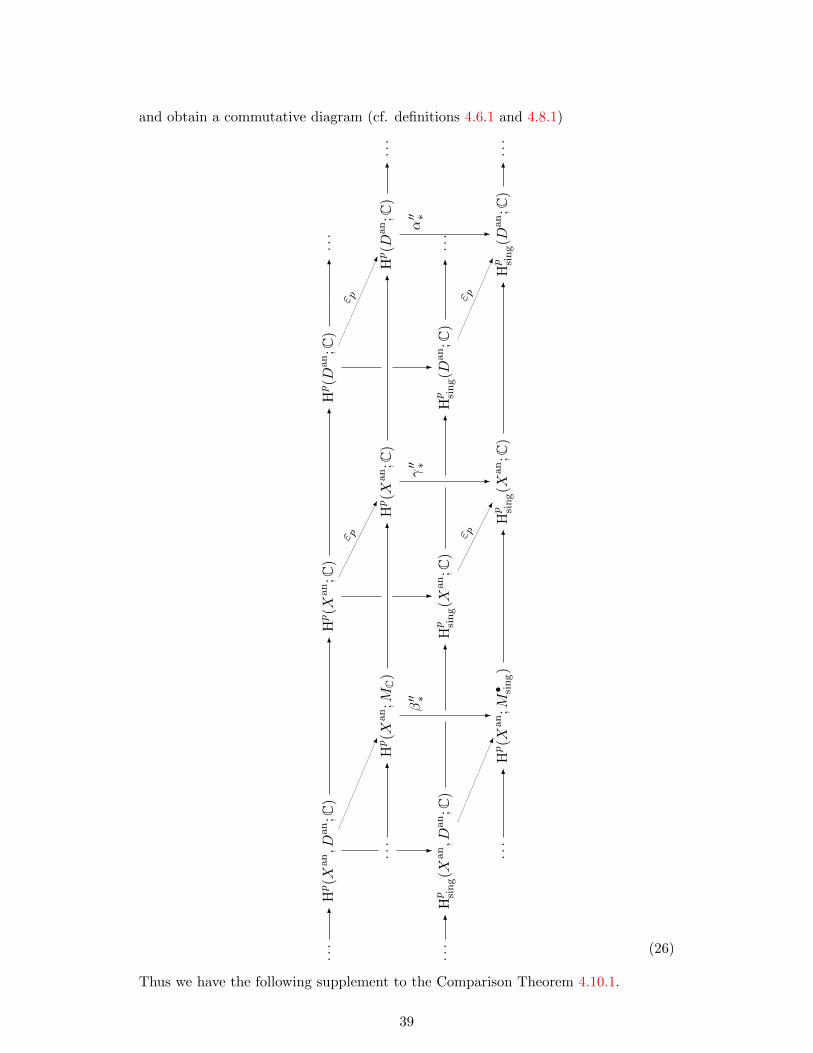
(26)

Thus we have the following supplement to the Comparison Theorem 4.10.1.

39

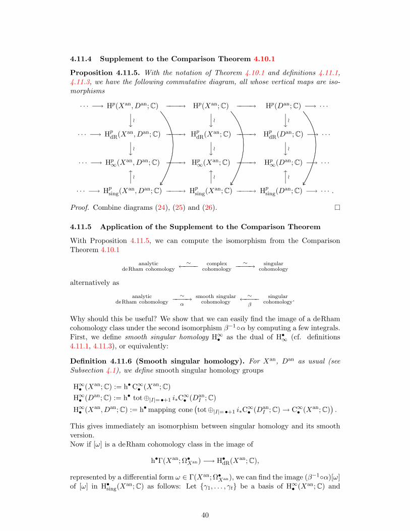
4.11.4 Supplement to the Comparison Theorem 4.10.1

Proposition 4.11.5. With the notation of Theorem 4.10.1 and definitions 4.11.1,4.11.3, we have the following commutative diagram, all whose vertical maps are iso-morphisms

· · · −→ Hp(Xan, Dan; C).

........................

.....

............................

............................

............................

............................

..........

..........

........

..........

..........

........

..............................

................................

..................................

....................................

......................................

. ...........

............

−−−−→ Hp(Xan; C).

........................

.....

............................

............................

............................

............................

..........

..........

........

..........

..........

........

..............................

................................

..................................

....................................

......................................

. ...........

............

−−−−→ Hp(Dan; C).

........................

.....

............................

............................

............................

............................

..........

..........

........

..........

..........

........

..............................

................................

..................................

....................................

......................................

. ...........

............

−→ · · ·yo yo yo· · · −→ Hp

dR(Xan, Dan; C) −−−−→ HpdR(Xan; C) −−−−→ Hp

dR(Dan; C) −→ · · ·yo yo yo· · · −→ Hp

∞(Xan, Dan; C) −−−−→ Hp∞(Xan; C) −−−−→ Hp

∞(Dan; C) −→ · · ·xo xo xo· · · −→ Hp

sing(Xan, Dan; C) −−−−→ Hp

sing(Xan; C) −−−−→ Hp

sing(Dan; C) −→ · · · .

Proof. Combine diagrams (24), (25) and (26).

4.11.5 Application of the Supplement to the Comparison Theorem

With Proposition 4.11.5, we can compute the isomorphism from the ComparisonTheorem 4.10.1

analyticdeRham cohomology

∼←−−−− complexcohomology

∼−−−−→ singularcohomology

alternatively as

analyticdeRham cohomology

∼−−−−→α

smooth singularcohomology

∼←−−−−β

singularcohomology.

Why should this be useful? We show that we can easily find the image of a deRhamcohomology class under the second isomorphism β−1α by computing a few integrals.First, we define smooth singular homology H∞• as the dual of H•∞ (cf. definitions4.11.1, 4.11.3), or equivalently:

Definition 4.11.6 (Smooth singular homology). For Xan, Dan as usual (seeSubsection 4.1), we define smooth singular homology groups

H∞• (Xan; C) := h•C∞• (Xan; C)H∞• (Dan; C) := h• tot⊕|I|= •+1 i∗C

∞• (Dan

I ; C)

H∞• (Xan, Dan; C) := h•mapping cone(tot⊕|I|= •+1 i∗C

∞• (Dan

I ; C)→ C∞• (Xan; C)).

This gives immediately an isomorphism between singular homology and its smoothversion.Now if [ω] is a deRham cohomology class in the image of

h•Γ(Xan; Ω•Xan) −→ H•dR(Xan; C),

represented by a differential form ω ∈ Γ(Xan; Ω•Xan), we can find the image (β−1α)[ω]of [ω] in H•sing(X

an; C) as follows: Let γ1, . . . , γt be a basis of H∞• (Xan; C) and

40

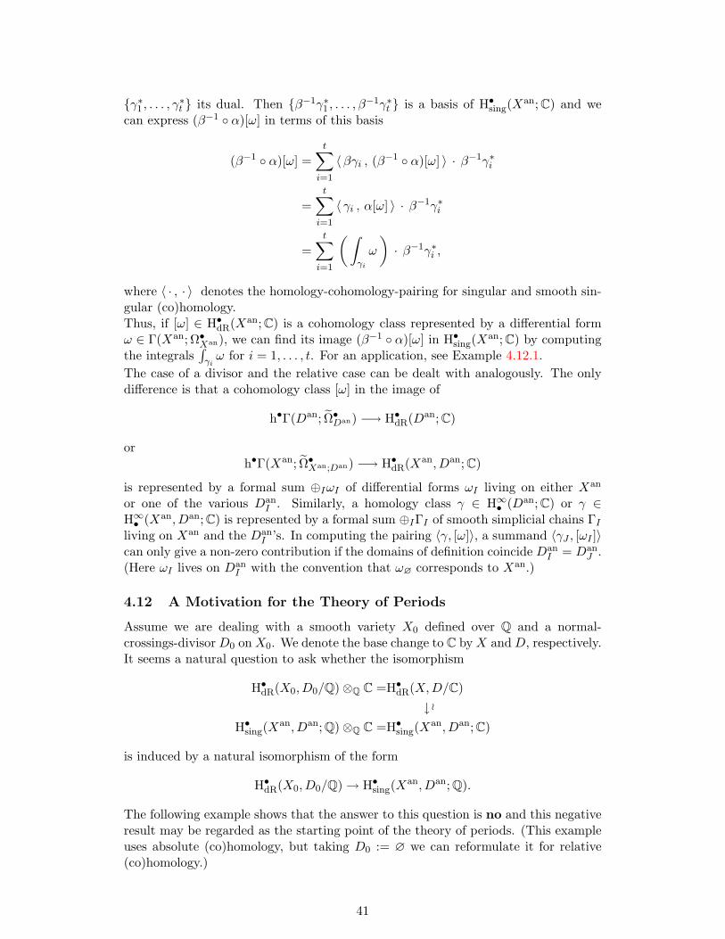
γ∗1 , . . . , γ∗t its dual. Then β−1γ∗1 , . . . , β−1γ∗t is a basis of H•sing(X

an; C) and wecan express (β−1 α)[ω] in terms of this basis

(β−1 α)[ω] =t∑i=1

〈βγi , (β−1 α)[ω] 〉 · β−1γ∗i

=t∑i=1

〈 γi , α[ω] 〉 · β−1γ∗i

=t∑i=1

(∫γi

ω

)· β−1γ∗i ,

where 〈 · , · 〉 denotes the homology-cohomology-pairing for singular and smooth sin-gular (co)homology.Thus, if [ω] ∈ H•dR(Xan; C) is a cohomology class represented by a differential formω ∈ Γ(Xan; Ω•Xan), we can find its image (β−1 α)[ω] in H•sing(X

an; C) by computingthe integrals

∫γiω for i = 1, . . . , t. For an application, see Example 4.12.1.

The case of a divisor and the relative case can be dealt with analogously. The onlydifference is that a cohomology class [ω] in the image of

h•Γ(Dan; Ω•Dan) −→ H•dR(Dan; C)

orh•Γ(Xan; Ω•Xan;Dan) −→ H•dR(Xan, Dan; C)

is represented by a formal sum ⊕IωI of differential forms ωI living on either Xan

or one of the various DanI . Similarly, a homology class γ ∈ H∞• (Dan; C) or γ ∈

H∞• (Xan, Dan; C) is represented by a formal sum ⊕IΓI of smooth simplicial chains ΓIliving on Xan and the Dan

I ’s. In computing the pairing 〈γ, [ω]〉, a summand 〈γJ , [ωI ]〉can only give a non-zero contribution if the domains of definition coincide Dan

I = DanJ .

(Here ωI lives on DanI with the convention that ω∅ corresponds to Xan.)

4.12 A Motivation for the Theory of Periods

Assume we are dealing with a smooth variety X0 defined over Q and a normal-crossings-divisorD0 onX0. We denote the base change to C byX andD, respectively.It seems a natural question to ask whether the isomorphism

H•dR(X0, D0/Q)⊗Q C =H•dR(X,D/C)↓ o

H•sing(Xan, Dan; Q)⊗Q C =H•sing(X

an, Dan; C)

is induced by a natural isomorphism of the form

H•dR(X0, D0/Q)→ H•sing(Xan, Dan; Q).

The following example shows that the answer to this question is no and this negativeresult may be regarded as the starting point of the theory of periods. (This exampleuses absolute (co)homology, but taking D0 := ∅ we can reformulate it for relative(co)homology.)

41

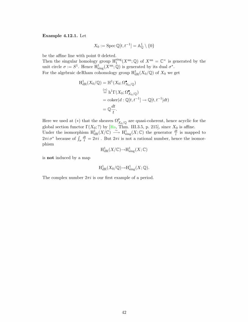
Example 4.12.1. Let

X0 := Spec Q[t, t−1] = A1Q \ 0

be the affine line with point 0 deleted.Then the singular homology group Hsing

1 (Xan; Q) of Xan = C× is generated by theunit circle σ := S1. Hence H1

sing(Xan; Q) is generated by its dual σ∗.

For the algebraic deRham cohomology group H1dR(X0/Q) of X0 we get

H1dR(X0/Q) = H1(X0; Ω•X0/Q)

(∗)= h1Γ(X0; Ω•X0/Q)

= coker(d : Q[t, t−1]→ Q[t, t−1]dt)

= Qdt

t.

Here we used at (∗) that the sheaves ΩpX0/Q are quasi-coherent, hence acyclic for the

global section functor Γ(X0; ?) by [Ha, Thm. III.3.5, p. 215], since X0 is affine.Under the isomorphism H1

dR(X/C) ∼−→ H1sing(X; C) the generator dt

t is mapped to2πi σ∗ because of

∫σdtt = 2πi . But 2πi is not a rational number, hence the isomor-

phismH1

dR(X/C)→H1sing(X; C)

is not induced by a map

H1dR(X0/Q)→H1

sing(X; Q).

The complex number 2πi is our first example of a period.

42

5 Definitions of Periods

A period is to be thought of as an integral that occurs in a geometric context. Intheir papers [K] and [KZ], Kontsevich and Zagier list various ways of how to define aperiod.It is stated in their papers without reference, that all these variants give the samedefinition. We give a partial proof of this statement in the Period Theorem 7.1.1.

5.1 First Definition of a Period: Pairing Periods

Let X0 be a smooth variety defined over Q and D0 a divisor with normal crossingson X0. We denote by Xan and Dan the complex analytic spaces (cf. Subsection 2.1)associated to the base change to C of X0 and D0.From the discussion of deRham cohomology in the previous sections (especially Pro-position 3.5.1 and Theorem 4.10.1), we see that inside the C-vector space Hp

dR(Xan, Dan; C)there sits a Q-lattice Hp

dR(X0, D0/Q) of full rank. Since

H•dR(Xan, Dan; C)(4.10.1)∼= H•sing(X

an, Dan; C) = H•sing(Xan, Dan; Q)⊗Q C,

the classical perfect pairing

〈·, ·〉 : Hsing• (Xan, Dan; Q)×H•sing(X

an, Dan; Q)→ Q

gives us a new non-degenerated pairing

〈·, ·〉 : Hsing• (Xan, Dan; Q)×H•dR(X0, D0/Q)→ C, (27)

which is natural in (X0, D0).

Definition 5.1.1 (Pairing period, short: p-period). The complex numbers

〈γ, ω0〉 ∈ C for ω0 ∈ H•dR(X0, D0/Q), γ ∈ Hsing• (Xan, Dan; Q),

which appear in the image of the natural pairing (27), are called p-periods. The setof all p-periods for all pairs (X0, D0) will be denoted by Pp.We call a p-period 〈γ, ω0〉 special or a p′-period, if ω0 is contained in the image of

h•Γ(X0; Ω•X0,D0/Q)→ H•dR(X0, D0/Q)

and write P ′p for the set of all special pairing periods for all X0, D0, ω0, γ.Running through bases

ω1, . . . , ωt of H•dR(X0, D0/Q) and γ1, . . . , γt of Hsing• (Xan, Dan; Q)

yields the so-called period matrix P :=(〈γi, ωj〉

)ti,j=1

of (X0, D0).

Remark 5.1.2. As a consequence of the Comparison Theorem 4.10.1, the periodmatrix must be a square matrix (cf. [K, p. 63]). In loc. cit. also a statement aboutits determinant is made, being a square root of a rational number times a power of2πi

determinant = ±√a · (2πi)n for a ∈ Q×, n ∈ N0.

An indication of a proof is not given there.

43

5.2 Second Definition of a Period: Abstract Periods

There exists another definition of a period, which also emphasizes their geometricorigin but does not involve algebraic deRham cohomology.For this definition the following data is needed,

• X0 a smooth algebraic variety defined over Q of dimension d,

• D0 a divisor on X0 with normal crossings,

• ω0 ∈ Γ(X0; ΩdX0/Q) an algebraic differential form of top degree,

• γ ∈ Hsingd (Xan, Dan; Q) a homology class of singular chains on the complex

manifold Xan with boundary on the divisor Dan.

As usual, we denote by Xan and Dan the complex analytic spaces (cf. Subsection 2.1)associated to the base change to C of X0 and D0. Thus, we are dealing with objectsXan, Dan and γ of real dimension 2d, 2d− 2 and d, respectively.The differential form ω0 on X0 gives rise to a differential form

ω := π∗ω0

on the base change X = X0 ×Q C, where π : X → X0 is the natural projection. Nowω0 is closed for dimension reasons, hence ω is closed as well.We choose a representative Γ ∈ α−1γ of the preimage α−1γ of γ under the isomor-phism (cf. Proposition 4.11.5)

α : H∞d (Xan, Dan; Q) ∼−→ Hsingd (Xan, Dan; Q)

and define ∫γω :=

∫Γd

ω,

where the chain Γd consists of the d-simplices of Γ (that is we ignore those d− q− 1-simplices of Γ that live on one of the Dan

I for |I| = q+ 1, q ≥ 0 — see page 12 for thedefinition of DI).

Observe that this integral∫γ ω is well-defined. The restriction of ω to some irreducible

component Danj of Dan is a holomorphic d-form on a complex manifold of dimension

d − 1, hence zero. Therefore the integral∫4 ω evaluates to zero for smooth singular

simplices 4 that are supported on Dan. Now if Γ′, Γ′′ are two representatives forα−1γ, we have

Γ′d − Γ′′d ∼ ∂(Γd+1)

modulo simplices living on some DanI for a smooth singular chain Γ of dimension d+1

Γ ∈ C∞d+1(Xan, Dan; Q).

Using Stoke’s theorem we get∫Γ′

d

ω −∫

Γ′′d

ω =∫∂(Γd+1)

ω =∫

Γd+1

dω = 0,

since ω is closed.

44

Definition 5.2.1 (Abstract period, short: a-period). We will call the complexnumber

∫γ ω the a-period of the quadruple (X0, D0, ω0, γ) and denote the set of all

a-periods for all (X0, D0, ω0, γ) by Pa.

Remark 5.2.2. This definition was motivated by Kontsevich’s discussion of effectiveperiods [K, def. 20, p. 62], which we will partly quote in subsection 7.3. ModuloConjecture 7.3.4, abstract and effective periods are essentially the same.

We can ask whether a different definition of the tuples (X0, D0, ω0, γ) yields moreperiod values. A partial answer is given by the following remarks.

Remark 5.2.3. (cf. [K, p. 62]) For example, we could have considered algebraicvarieties defined over Q. However, doing so does not give us more period values.

Proof.

• Any variety X0 defined over Q is already defined over a finite extensionQ ′ of Q, i.e. there exists a variety X ′0 such that

X0 = X ′0 ×Q ′ Q.

ViaX ′0 −→ Spec Q ′ −→ Spec Q

we may consider X ′0 as a variety defined over Q.

• An analogous argument applies to a normal-crossings-divisor D0 on X0.By possibly replacing Q ′ by a finite extension field, we can thereforeassume w.l.o.g. that D0 is the base extension of a normal-crossings-divisorD ′0 on X ′0

D0 = D ′0 ×Q Q.

• Also any differential d-form ω0 ∈ Γ(X0; ΩdX0/Q

) can be considered as adifferential form ω′0 on X ′0 by eventually replacing Q ′ by a finite extension.

Finally, we discuss singular homology classes.

• First observe that

|Spec C⊗Q Q ′| = HomC(C⊗Q Q ′,C)= HomQ(Q ′,C)

is a finite discrete set of points. Thus X ′ is a finite union of disjoint copiesof X

X ′ = X ′0 ×Q C= X ′0 ×Q ′ Q ′ ×Q C×C C= (X ′0 ×Q ′ C)×C

(Q ′ ×Q C)

)= X ×HomQ(Q ′,C)

=∐

σ : Q ′→CX.

45

Similarly, D ′ =∐σD. Therefore we have

Hsingd (X ′ an, D ′ an; Q) =

⊕σ

Hsingd (Xan, Dan; Q).

If γ ∈ Hsingd (Xan, Dan; Q) is some singular homology class, we can pick

any σ′ : Q ′ → C and find

γ′ := σ′ × γ ∈ Hsingd (X ′ an, D ′ an; Q) = ⊕σ Hsing

d (Xan, Dan; Q).

Now ∫γ′ω′ =

∫γω

which finishes the proof.

Remark 5.2.4. (cf. [K, p. 62]) The requirement of X to be smooth was also madeonly for convenience and is not a real restriction.

We postpone the proof of Remark 5.2.4 until the Period Theorem 7.1.1 is proved.

5.3 Third Definition of a Period: Naıve Periods

For the last definition of a period, we need the notion of semi-algebraic sets.Let K be any field contained in R.

Definition 5.3.1 (K-semi-algebraic sets, [Hi2, Def. 1.1, p. 166]). A subset ofRn is said to be K-semi-algebraic, if it is of the form

x ∈ Rn|f(x) ≥ 0

for some polynomial f ∈ K[x1, . . . , xn] or can be obtained from sets of this formin a finite number of steps, where each step consists of one of the following basicoperations:

(i) complementary set,

(ii) finite intersection,

(iii) finite union.

Denote the integral closure of Q in R by Q. Note that Q is a field. Now we candefine

Definition 5.3.2 (Naıve periods, short: n-periods). Let

• G ⊆ Rn be an oriented compact Q-semi-algebraic set which is equidimen-sional of dimension d, and

• ω0 a rational differential d-form on Rn having coefficients in Q, whichdoes not have poles on G.

Then we call the complex number∫G ω0 a n-period and denote the set of all n-periods

for all G and ω0 by Pn.

This set Pn enjoys additional structure.

46

Proposition 5.3.3. The set Pn is a Q-algebra.

Proof. Additive structure: Let∫G1ω1 and

∫G2ω2 ∈ Pn be periods with domains of

integration G1 ⊆ Rn1 and G2 ⊆ Rn2 . Using the inclusions

i1 : Rn1 ∼= Rn1 × 1/2 × 0 ⊂ Rn1 × R× Rn2 andi2 : Rn2 ∼= 0 × −1/2 × Rn2 ⊂ Rn1 × R× Rn2 ,

we can write i1(G1)∪i2(G2) for the disjoint union of G1 and G2. With the projectionspj : Rn1×R×Rn2 → Rnj for j = 1, 2, we can lift ωj on Rnj to p∗jωj on Rn1×R×Rn2 .For q1, q2 ∈ Q we get

q1

∫G1

ω1 + q2

∫G2

ω2 =∫i1(G1)∪i2(G2)

q1 · (1/2 + t) · p∗1ω1 + q2 · (1/2− t) · p∗2ω2 ∈ Pn,

where t is the coordinate of the “middle” factor R of Rn1 ×R×Rn2 . This shows thatPn is a Q-vector space.Multiplicative structure: In order to show that Pn is closed under multiplication, wewrite

pi : Rn1 × Rn2 −→ Rni , i = 1, 2

for the natural projections and obtain(∫G1

ω1

)·(∫

G2

ω2

)=∫G1×G2

p∗1ω1 ∧ p∗2ω2 ∈ Pn

by the Fubini formula.

Remark 5.3.4. The Definition 5.3.2 was inspired by the one given in [KZ, p. 772]

Definition. A [naıve] period is a complex number whose real andimaginary part are values of absolutely convergent integrals of ratio-nal functions with rational coefficients, over domains in Rn givenby polynomial inequalities with rational coefficients.

We will not work with this definition and use the modified version 5.3.2 instead, sincethis gives us more flexibility in proofs.From the statements made in [KZ, p. 773] it would follow that both definitions of anaıve period agree.

Examples of naıve periods are

•∫ 2

1

dt

t= ln 2,

•∫ 1

0

1t2 + 1

dt = π and

•∫G

dt

s=∫ 2

1

dt√t3 + 1

= elliptic integrals,

for G := (t, s) ∈ R2 | 1 ≤ t ≤ 2, 0 ≤ s, s2 = t3 +1.

As a problematic example, we consider the following identity.

47

Proposition 5.3.5 (cf. [K, p. 62]). We have∫0≤ t1≤ t2≤ 1

dt1 ∧ dt2(1− t1) t2

= ζ(2). (28)

Proof. This equality follows by a simple power series manipulation: For 0 ≤ t2 < 1,we have ∫ t2

0

dt11− t1

= − log(1− t2) =∞∑n=1

tn2n.

Let ε > 0. The power series∑∞

n=1tn−12n converges uniformly for 0 ≤ t2 ≤ 1 − ε and

we get ∫0≤ t1≤ t2≤ 1−ε

dt1 dt2(1− t1) t2

=∫ 1−ε

0

∞∑n=1

tn−12

ndt2 =

∞∑n=1

(1− ε)n

n2.

Applying Abel’s Theorem [Fi, vol. 2, XII, 438, 6, p. 411] at (∗), using∑∞

n=11n3 <∞

gives us ∫0≤ t1≤ t2≤ 1

dt1 dt2(1− t1) t2

= limε→0

∞∑n=1

(1− ε)n

n2

(∗)=∞∑n=1

1n2

= ζ(2).

Equation (28) is not a valid representation of ζ(2) as an integral for a naıve period inour sense, because the pole locus t1 = 1 ∪ t2 = 0 of t1 ∧ t2

(1−t1) t2is not disjoint with

the domain of integration 0 ≤ t1 ≤ t2 ≤ 1. But (28) gives a valid period integralaccording to the original definition of [KZ, p. 772] — see Remark 5.3.4. We will showin Example 8.4 how to circumvent this difficulty.

We will prove in the Period Theorem 7.1.1, that special pairing, abstract and naıveperiods are essentially the same, i.e.

P ′p = Pa = Pn,

but have to make a digression on the triangulation of varieties first.Note that in Subsection 7.3 we will give a fourth definition of a period.

48

6 Triangulation of Algebraic Varieties

If X0 is a variety defined over Q we may ask whether any singular homology classγ ∈ Hsing

• (Xan; Q) can be represented by an object described by polynomials. This isindeed the case: For a precise statement we need several definitions. The result willbe formulated in Proposition 6.2.2.

6.1 Semi-algebraic Sets

We already defined Q-semi-algebraic sets in Definition 5.3.1.

Definition 6.1.1 (Q-semi-algebraic map [Hi2, p. 168]). A continuous map fbetween Q-semi-algebraic sets A ⊆ Rn and B ⊆ Rm is said to be Q-semi-algebraic ifits graph

Γf :=(a, f(a)

)| a ∈ A

⊆ A×B ⊆ Rn+m

is Q-semi-algebraic.

Example 6.1.2. Any polynomial map

f : A −→ B

(a1, . . . , an) 7→ (f1(a1, . . . , an), . . . , fm(a1, . . . , an))

between Q-semi-algebraic sets A ⊆ Rn and B ⊆ Rm with fi ∈ Q[x1, . . . , xn] fori = 1, . . . ,m is Q-semi-algebraic, since it is continuous and its graph Γf ⊆ Rn+m iscut out from A×B by the polynomials

yi − fi(x1, . . . , xn) ∈ Q[x1, . . . , xn, y1, . . . , ym] for i = 1, . . . ,m. (29)

We can even allow f to be a rational map with rational component functions

fi ∈ Q(x1, . . . , xn), i = 1, . . . ,m

as long as none of the denominators of the fi vanish at a point of A. The argu-ment remains the same except that the expression (29) has to be multiplied by thedenominator of fi.

Fact 6.1.3 ([Hi2, Prop. II, p. 167], [Sb, Thm. 3, p. 370]). By a result ofSeidenberg-Tarski, the image (respectively preimage) of a Q-semi-algebraic set undera Q-semi-algebraic map is again Q-semi-algebraic.

As the name suggests any algebraic set should be in particular Q-semi-algebraic.

Lemma 6.1.4. Let X0 be an algebraic variety defined over Q. Then we can regardthe complex analytic space Xan(cf. Subsection 2.1) associated to the base changeX = X0 ×eQ C as a bounded Q-semi-algebraic subset

Xan ⊆ RN (30)

for some N . Moreover, if f0 : X0 → Y0 is a morphism of varieties defined over Q,we can consider fan : Xan → Y an as a Q-semi-algebraic map.

49

Proof. First step X0 = QPn: Consider

• CPnan with homogenous coordinates x0, . . . , xn, which we split as xm =am + ibm with am, bm ∈ R in real and imaginary part, and

• RN , N = 2(n+ 1)2, with coordinates ykl, zklk,l=0,...,n.

We define a map

ψ : CPnan[x0:...:xn]

−→ RN

(y00,z00,...,ynn,znn)

[x0 : . . . : xn] 7→(. . . ,

Rexkxl∑nm=0 |xm|2︸ ︷︷ ︸ykl

,Imxkxl∑nm=0 |xm|2︸ ︷︷ ︸zkl

, . . .

)

[a0 + ib0 : . . . : an + ibn] 7→(. . . ,

akal + bkbl∑nm=0 a

2m + b2m︸ ︷︷ ︸

ykl

,bkal − akbl∑nm=0 a

2m + b2m︸ ︷︷ ︸

zkl

, . . .

).

Rewriting the last line (with the convention 0 · cos( indeterminateangle ) = 0) as

[r0eiφ0 : . . . : rneiφn ] 7→(. . . ,

rkrl cos(φk − φl)∑nm=0 r

2m

,rkrl sin(φk − φl)∑n

m=0 r2m

, . . .

)(31)

shows that ψ is injective: Assume

ψ([r0eiφ0 : . . . : rneiφn ]

)= (y00, z00, . . . , ynn, znn)

where rk 6= 0, or equivalently ykk 6= 0, for a fixed k. We find

rlrk

=

√y2kl + z2

kl

ykk, and

φk − φl =

arctan(zkl/ykl) if ykl 6= 0,π/2 if ykl = 0, zkl > 0,indeterminate if ykl = zkl = 0,−π/2 if ykl = 0, zkl < 0;

that is the preimage of (y00, z00, . . . , ynn, znn) is uniquely determined.Therefore we can consider CPnan via ψ as a subset of RN . It is bounded since it iscontained in the unit sphere SN−1 ⊂ RN . We claim that ψ(CPnan) is also Q-semi-algebraic. The composition of the projection

π : R2(n+1) \ (0, . . . , 0) −→ CPnan(a0, b0, . . . , an, bn) 7→ [a0 + ib0 : . . . : an + ibn]

with the map ψ is a polynomial map, hence Q-semi-algebraic by Example 6.1.2. Thus

imψ π = imψ ⊆ RN

is Q-semi-algebraic by Fact 6.1.3.

50

Second step (zero set of a polynomial): We use the notation

V (g) := x ∈ CPnan | g(x) = 0 for g ∈ C[x0, . . . , xn] homogenous, and

W (h) := t ∈ RN |h(t) = 0 for h ∈ C[y00, . . . , znn].

Let Xan = V (g) for some homogenous g ∈ Q[x0, . . . , xn]. Then ψ(Xan) ⊆ RN is aQ-semi-algebraic subset, as a little calculation shows. Setting for k = 0, . . . , n

gk := “g(xxk)”= g(x0xk, . . . , xnxk)= g((a0ak + b0bk) + i(b0ak − a0bk), . . . , (anak + bnbk) + i(bnak − anbk)

),

where xj = aj + ibj for j = 0, . . . , n, and

hk := g(y0k + iz0k, . . . , ynk + iznk),

we obtain

ψ(Xan) = ψ(V (g))

=n⋂k=0

ψ(V (gk))

=n⋂k=0

ψ(CPnan) ∩W (hk)

=n⋂k=0

ψ(CPnan) ∩W (Rehk) ∩W (Imhk).

Final step: We can choose an embedding

X0 ⊆ QPn,

thus gettingXan ⊆ CPnan.

Since X0 is a locally closed subvariety of QPn, Xan can be expressed in terms ofsubvarieties of the form V (g) with g ∈ Q[x0, . . . , xn], using only the following basicoperations

(i) complementary set,

(ii) finite intersection,

(iii) finite union.

Now Q-semi-algebraic sets are stable under these operations as well and the firstassertion is proved. Second assertion: The first part of the lemma provides us with Q-semi-algebraicinclusions

ψ : Xan ⊆ CPnanx=[x0:...:xn]

⊆ RN

(y00,z00,...,ynn,znn),

φ : Y an ⊆ CPmanu=[u0:...:um]

⊆ RM

(v00,w00,...,vmm,wmm),

51

and a choice of coordinates as indicated. We use the notation

V (g) := (x, u) ∈ CPnan × CPman | g(x, u) = 0,for g ∈ C[x0, . . . , xn, u0, . . . , um] homogenous in both x and u, and

W (h) := t ∈ RN+M |h(t) = 0, for h ∈ C[y00, . . . , znn, v00, . . . , wmm].

Let Ui be a finite open affine covering of X0 such that f0(Ui) satisfies

• f0(Ui) does not meet the hyperplane uj = 0 ⊂ QPm for some j, and

• f0(Ui) is contained in an open affine subset Vi of Y0.

This is always possible, since we can start with the open covering Y0∩uj 6= 0 of Y0,take a subordinated open affine covering Vi′, and then choose a finite open affinecovering Ui subordinated to f−1(Vi′). Now each of the maps

fi := fan|Ui: Uan

i −→ Y an

has image contained in V ani and does not meet the hyperplane u ∈ CPman |uj = 0

for an appropriate jfi : Uan

i −→ V ani .

Being associated to an algebraic map between affine varieties, this map is rational

fi : x 7→

[g′0(x)g′′0(x)

: . . . :g′j−1(x)g′′j−1(x)

: 1j

:g′j+1(x)g′′j+1(x)

: . . . :g′m(x)g′′m(x)

],

with g′k, g′′k ∈ Q[x0, . . . , xn], k = 0, . . . , j, . . . ,m. Since the graph Γfan of fan is the

finite union of the graphs Γfiof the fi, it is sufficient to prove that (ψ × φ)(Γfi

) is aQ-semi-algebraic subset of RN+M . Now

Γfi= (Uan

i × V ani )∩

n⋂k=0k 6=j

V

(ykyj−g′k(x)g′′k(x)

)= (Uan

i × V ani )∩

n⋂k=0k 6=j

V (ykg′′k(x)−yjg′k(x)),

so all we have to deal with is

V (ykg′′k(x)− yjg′k(x)).

Again a little calculation is necessary. Setting

gpq := “ukuqg′′k(xxp)− ujuqg′k(xxp)”= ukuqg

′′k(x0xp, . . . , xnxp)− ujuqg′k(x0xp, . . . , xnxp)

=((ckcq + dkdq) + i(dkcq − ckdq)

)g′′k((a0ap + b0bp) + i(b0ap − a0bp), . . . , (anap + bnbp) + i(bnap − anbp)

)−((cjcq + djdq) + i(djcq − cjdq)

)g′k((a0ap + b0bp) + i(b0ap − a0bp), . . . , (anap + bnbp) + i(bnap − anbp)

),

where xl = al + ibl for l = 0, . . . , n, ul = cl + idl for l = 0, . . . ,m, and

hpq := (vkq+iwkq)g′′k(y0p+iz0p, . . . , ynp+iznp)−(vjq+iwjq)g′k(y0p+iz0p, . . . , ynp+iznp),

52

we obtain

(ψ × φ)(V(ykg′′k(x)−yjg′k(x)

))=

=n⋂p=0

m⋂q=0

(ψ × φ)(V (gpq))

=n⋂p=0

m⋂q=0

(ψ × φ)(Uani × V an

j ) ∩W (hpq)

=n⋂p=0

m⋂q=0

(ψ × φ)(Uani × V an

j ) ∩W (Rehpq) ∩W (Imhpq).

6.2 Semi-algebraic Singular Chains

We need further prerequisites in order to state the announced Proposition 6.2.2.

Definition 6.2.1 (Open simplex, [Hi2, p. 168]). By an open simplex 4 wemean the interior of a simplex (= the convex hull of r+ 1 points in Rn which span ar-dimensional subspace). For convenience, a point is considered as an open simplexas well.The notation 4std

d will be reserved for the closed standard simplex spanned by thestandard basis (0, . . . , 0, 1

i, 0, . . . , 0) | i = 1, . . . , d+ 1 of Rd+1.

Consider the following data (∗):

• X0 a variety defined over Q,

• D0 a divisor on X0 with normal crossings,

• and finally γ ∈ Hsingp (Xan, Dan; Q), p ∈ N0.

As usual, we have denoted by Xan (resp. Dan) the complex analytic space associatedto the base change X = X0 ×eQ C (resp. D = D0 ×eQ C).

By Lemma 6.1.4, we may consider both Xan and Dan as bounded Q-semi-algebraicsubsets of RN .We are now able to formulate our proposition.

Proposition 6.2.2. With data (∗) as above, we can find a representative of γ that isa rational linear combination of singular simplices each of which is Q-semi-algebraic.

The proof of this proposition relies on the following proposition due to Lojasiewiczwhich has been written down by Hironaka.

Proposition 6.2.3 (Triangulation of Q-semi-algebraic sets, [Hi2, p. 170]).For Xi a finite system of bounded Q-semi-algebraic sets in Rn, there exists a sim-plicial decomposition

Rn =∐j

4j

by open simplices 4j and a Q-semi-algebraic automorphism

κ : Rn → Rn

such that each Xi is a finite union of some of the κ(4j).

53

Note 6.2.4. Although Hironaka considers R-semi-algebraic sets, it has been checkedby the author, that we can safely replace R by Q in his article (including the facthe cites from [Sb]). The only problem that could possibly arise concerns a “gooddirection lemma”:

Lemma 6.2.5 (Good direction lemma for R, [Hi2, p. 172], [KB, Thm. 5.I,p. 242]). Let Z be a R-semi-algebraic subset of Rn, which is nowhere dense. Adirection v ∈ |RPn−1| is called good, if any line l in Rn parallel to v meets Z in adiscrete (maybe empty) set of points; otherwise v is called bad. Then the set B(Z) ofbad directions is a Baire category set in |RPn−1|.

This gives immediately good directions v ∈ |RPn−1| \ B(Z), but not necessarilyv ∈ |QPn−1| \ B(Z). However, in Remark 2.1 of [Hi2], which follows directly afterthe lemma, the following statement is made: If Z is compact, then B(Z) is closed in|RPn−1|. In particular |QPn−1| \ B(Z) will be non-empty. Since we only considerbounded Q-semi-algebraic sets Z ′, we may take Z := Z ′ (which is compact by Heine-Borel), and thus find a good direction v ∈ |QPn−1| \B(Z ′) using B(Z ′) ⊆ B(Z).

Lemma 6.2.6 (Good direction lemma for Q). Let Z ′ be a bounded Q-semi-algebraic subset of Rn, which is nowhere dense. Then the set |QPn−1| \B(Z) of gooddirections is non-empty.

Proof of Proposition 6.2.2. Applying Proposition 6.2.3 to the two-element system ofQ-semi-algebraic sets Xan, Dan ⊆ RN , we obtain a Q-semi-algebraic decomposition

RN =∐j

4j

of RN by open simplices 4j and a Q-semi-algebraic automorphism

κ : RN → RN .

We write 4j for the closure of 4j . The sets

K := 4j |κ(4j) ⊆ Xan and L := 4j |κ(4j) ⊆ Dan

can be thought of as finite simplicial complexes, but built out of open simplices insteadof closed ones. We define their geometric realizations

|K| :=⋃4j∈K

4j and |L| :=⋃4j∈L

4j .

Then Proposition 6.2.3 states that κ maps the pair of topological spaces (|K|, |L|)homeomorphically to (Xan, Dan).Easy case: If X0 is complete, so is X (by [Ha, Cor. II.4.8(c), p. 102]), hence Xan andDan will be compact [Ha, B.1, p. 439]. In this situation

K := 4j |κ(4j) ⊆ Xan and L := 4j |κ(4j) ⊆ Dan

are (ordinary) simplicial complexes, whose geometric realizations coincide with thoseof K and L, respectively. In particular

Hsimpl• (K,L; Q) ∼= Hsing

• (∣∣K∣∣ , ∣∣L∣∣ ; Q)

∼= Hsing• (|K|, |L|; Q)

∼= Hsing• (Xan, Dan; Q).

(32)

54

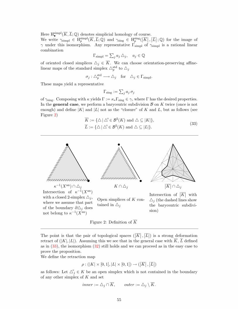
Here Hsimpl• (K,L; Q) denotes simplicial homology of course.

We write γsimpl ∈ Hsimplp (K,L; Q) and γsing ∈ Hsing

p (∣∣K∣∣ , ∣∣L∣∣ ; Q) for the image of

γ under this isomorphism. Any representative Γsimpl of γsimpl is a rational linearcombination

Γsimpl =∑

j aj4j , aj ∈ Q

of oriented closed simplices 4j ∈ K. We can choose orientation-preserving affine-linear maps of the standard simplex 4std

p to 4j

σj : 4stdp −→ 4j for 4j ∈ Γsimpl.

These maps yield a representative

Γsing :=∑

j aj σj

of γsing. Composing with κ yields Γ := κ∗Γsing ∈ γ, where Γ has the desired properties.In the general case, we perform a barycentric subdivision B on K twice (once is notenough) and define |K| and |L| not as the “closure” of K and L, but as follows (seeFigure 2)

K := 4 |4∈ B2(K) and 4 ⊆ |K|,L := 4 |4∈ B2(K) and 4 ⊆ |L|.

(33)

κ−1(Xan) ∩4j K ∩4j

∣∣K∣∣ ∩4j

Intersection of κ−1(Xan)with a closed 2-simplex4j ,where we assume that partof the boundary ∂4j doesnot belong to κ−1(Xan)

Open simplices of K con-tained in 4j

Intersection of∣∣K∣∣ with

4j (the dashed lines showthe barycentric subdivi-sion)

Figure 2: Definition of K

The point is that the pair of topological spaces (∣∣K∣∣ , ∣∣L∣∣) is a strong deformation

retract of (|K|, |L|). Assuming this we see that in the general case with K, L definedas in (33), the isomorphism (32) still holds and we can proceed as in the easy case toprove the proposition.We define the retraction map

ρ : (|K| × [0, 1], |L| × [0, 1])→ (∣∣K∣∣ , ∣∣L∣∣)

as follows: Let 4j ∈ K be an open simplex which is not contained in the boundaryof any other simplex of K and set

inner := 4j ∩K, outer := 4j \K.

55

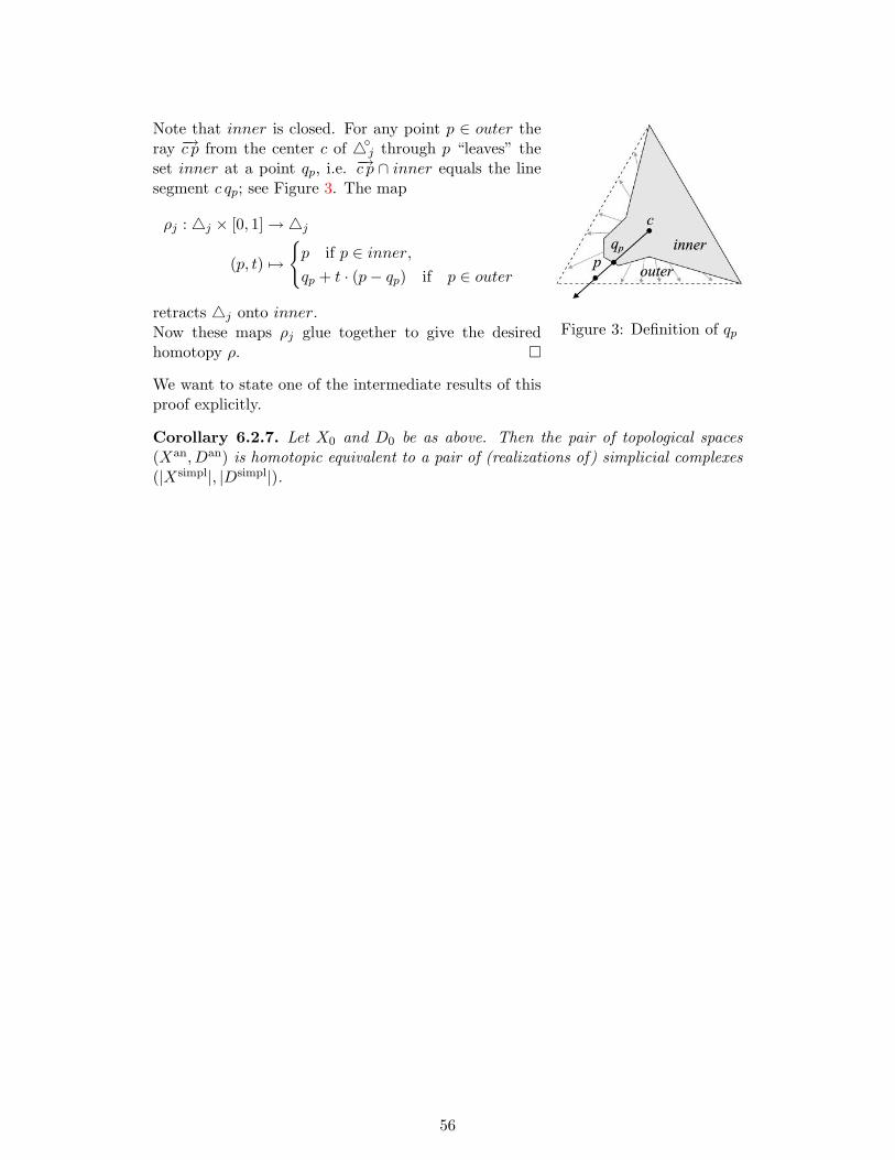
Figure 3: Definition of qp

Note that inner is closed. For any point p ∈ outer theray −→c p from the center c of 4j through p “leaves” theset inner at a point qp, i.e. −→c p ∩ inner equals the linesegment c qp; see Figure 3. The map

ρj : 4j × [0, 1]→4j

(p, t) 7→

p if p ∈ inner,qp + t · (p− qp) if p ∈ outer

retracts 4j onto inner.Now these maps ρj glue together to give the desiredhomotopy ρ.

We want to state one of the intermediate results of thisproof explicitly.

Corollary 6.2.7. Let X0 and D0 be as above. Then the pair of topological spaces(Xan, Dan) is homotopic equivalent to a pair of (realizations of) simplicial complexes(|Xsimpl|, |Dsimpl|).

56

7 Periods Revisited

7.1 Comparison of Definitions of Periods

We are now ready to prove the theorem announced in the introduction.

Main Theorem 7.1.1 (Period theorem). It holds

P ′p = Pa = Pn,

that is the following three definitions of a period given in Section 5 coincide

• special pairing periods (cf. Definition 5.1.1),

• abstract periods (cf. Definition 5.2.1), and

• naıve periods (cf. Definition 5.3.2).

Note that we will give a fourth definition of a period in Subsection 7.3.

Proof. Pa ⊆ P ′p: Let∫γ ω ∈ Pa be an abstract period coming from (X0, D0, ω0, γ).

We want to understand ω0 as an element of Γ(X0; ΩdX0,D0/Q) = Γ(X0; Ωd

X0/Q) ⊕Γ(D0; Ωd−1

D0/Q) via Γ(X0; ΩdX0/Q) Γ(X0; Ωd

X0,D0/Q), where d := dimX0. Then

ω0 ∈ Γ(X0; Ω•X0,D0/Q) is a cocycle, since ω0 is closed (for dimension reasons) andits restriction to each of the irreducible components Dj of D0 is zero (also for dimen-sion reasons). Thus we can consider [ω0] via

h•Γ(X0; Ω•X0,D0/Q)→ H•dR(X0, D0/Q)

as an algebraic deRham cohomology class and find (cf. Subsection 4.11.5)∫γω = 〈γ, [ω0]〉 ∈ P ′p.

P ′p ⊆ Pn: As explained in Subsection 4.11.5, a special pairing period

〈γ, ω0〉 ∈ P ′p

is a sum of integrals ∑I〈γI , ωI〉 =

∑I

∫γIωI ,

where ωI ∈ H•dR(DI/Q) and γI ∈ H•∞(DI ; Q). Since Pn is closed under addition byProposition 5.3.3, it suffices to prove

∫γIωI ∈ Pn for all index sets I.

We choose an embeddingDI ⊆ QPn

(x0:...:xn)

and equip QPn with coordinates as indicated. Lemma 6.1.4 provides us with a map

ψ : CPnan → RN

such that DanI and CPnan become Q-semi-algebraic subsets of RN . Then, by Proposi-

tion 6.2.2, ψ∗γI has a representative which is a rational linear combination of singularsimplices Γi, each of which is Q-semi-algebraic.

57

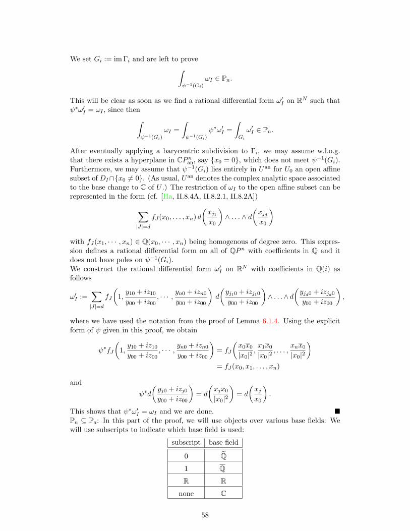
We set Gi := im Γi and are left to prove∫ψ−1(Gi)

ωI ∈ Pn.

This will be clear as soon as we find a rational differential form ω′I on RN such thatψ∗ω′I = ωI , since then∫

ψ−1(Gi)ωI =

∫ψ−1(Gi)

ψ∗ω′I =∫Gi

ω′I ∈ Pn.

After eventually applying a barycentric subdivision to Γi, we may assume w.l.o.g.that there exists a hyperplane in CPnan, say x0 = 0, which does not meet ψ−1(Gi).Furthermore, we may assume that ψ−1(Gi) lies entirely in Uan for U0 an open affinesubset of DI∩x0 6= 0. (As usual, Uan denotes the complex analytic space associatedto the base change to C of U .) The restriction of ωI to the open affine subset can berepresented in the form (cf. [Ha, II.8.4A, II.8.2.1, II.8.2A])∑

|J |=d

fJ(x0, . . . , xn) d(xj1x0

)∧ . . . ∧ d

(xjdx0

)

with fJ(x1, · · · , xn) ∈ Q(x0, · · · , xn) being homogenous of degree zero. This expres-sion defines a rational differential form on all of QPn with coefficients in Q and itdoes not have poles on ψ−1(Gi).We construct the rational differential form ω′I on RN with coefficients in Q(i) asfollows

ω′I :=∑|J |=d

fJ

(1,y10 + iz10

y00 + iz00, · · · , yn0 + izn0

y00 + iz00

)d

(yj10 + izj10

y00 + iz00

)∧ . . .∧ d

(yjd0 + izjd0

y00 + iz00

),

where we have used the notation from the proof of Lemma 6.1.4. Using the explicitform of ψ given in this proof, we obtain

ψ∗fJ

(1,y10 + iz10

y00 + iz00, · · · , yn0 + izn0

y00 + iz00

)= fJ

(x0x0

|x0|2,x1x0

|x0|2, . . . ,

xnx0

|x0|2

)= fJ(x0, x1, . . . , xn)

and

ψ∗d

(yj0 + izj0y00 + iz00

)= d

(xjx0

|x0|2

)= d

(xjx0

).

This shows that ψ∗ω′I = ωI and we are done. Pn ⊆ Pa: In this part of the proof, we will use objects over various base fields: Wewill use subscripts to indicate which base field is used:

subscript base field

0 Q

1 Q

R R

none C

58

Furthermore, we fix an embedding Q ⊂ C.Let

∫G ωR ∈ Pn be a naıve period with

• G ⊂ Rn an oriented Q-semi-algebraic set, equidimensional of dimensiond, and

• ωR a rational differential d-form on Rn with coefficients in Q, which doesnot have poles on G.

The Q-semi-algebraic set G ⊂ Rn is given by polynomial inequalities and equalities.By omitting the inequalities but keeping the equalities in the definition of G, we seethat G is supported on (the set of R-valued points of) a variety YR ⊆ An

R of samedimension d. This variety YR is already defined over Q

YR = Y0 ×eQ R

for a variety Y0 ⊆ AneQ over Q. Similarly the boundary ∂G of G is supported on a

variety ER, likewise defined over Q

ER = E0 ×eQ R.

Note that E0 is a divisor on Y0. By eventually enlarging E0, we may assume w.l.o.g.that E0 contains the singular locus of Y0. In order to obtain an abstract period, weneed smooth varieties. The resolution of singularities according to Hironaka [Hi1]provides us with a Cartesian square

E0 ⊆ Y0

↓ ↓ π0

E0 ⊆ Y0

(34)

where

• Y0 is smooth and quasi-projective,

• π0 is proper, surjective and birational, and

• E0 is a divisor with normal crossings.

In fact, π0 is an isomorphism away from E0 since the singular locus of Y0 is containedin E0

π0|eU0

: U0∼−→ U0 (35)

with U0 := Y0 \ E0 and U0 := Y0 \ E0.We apply the functor an (associated complex analytic space — cf. Subsection 2.1)to the base change to C of the map π0 : Y0 → Y0 and obtain a projection

πan : Y an → Y an.

We want to show that the “strict transform” of G

G := π−1an (G \ Ean) ⊆ Y an

59

can be triangulated. Since CPnan is the projective closure of Cn, we have Cn ⊂ CPnanand thus get an embedding

Y an ⊆ Cn ⊂ CPnan.

We also choose an embeddingY an ⊆ CPman

for some m ∈ N. Using Lemma 6.1.4, we may consider both Y an and Y an as Q-semi-algebraic sets via some maps

ψ : Y an ⊂ CPnan → RN , and

ψ : Y an ⊆ CPman → RM .

In this setting, the induced projection

πan : Y an −→ Y an

becomes a Q-semi-algebraic map. The composition of ψ with the inclusion G ⊆ Y an

is a Q-semi-algebraic map; hence G ⊂ RN is Q-semi-algebraic by Fact 6.1.3. SinceEan is also Q-semi-algebraic via ψ, we find that G \ Ean is Q-semi-algebraic. Againby Fact 6.1.3, π−1

an (G \ Ean) ⊂ RM is Q-semi-algebraic. Thus G ⊂ RM , being theclosure of a Q-semi-algebraic set, is Q-semi-algebraic. From Proposition 6.2.2, we seethat G can be triangulated

G = ∪j4j , (36)

where the 4j are (homeomorphic images of) d-dimensional simplices.Our next aim is to define an algebraic differential form ω1 replacing ωR. We firstmake a base change in (34) from Q to Q and obtain

E1 ⊆ Y1

↓ ↓ π1

E1 ⊆ Y1 .

The differential d-form ωR can be written as

ωR =∑|J |=d

fJ(x1, . . . , xn) dxj1 ∧ . . . ∧ dxjd , (37)

where x1, . . . , xn are coordinates of Rn and fJ ∈ Q(x1, . . . , xn). We can use equation(37) to define a differential form ω1 on An

Q

ωR =∑|J |=d

fJ(x1, . . . , xn) dxj1 ∧ . . . ∧ dxjd ,

where now x1, . . . , xn denote coordinates of AnQ. The pole locus of ω1 gives us a variety

Z1 ⊂ AnQ. We set

X1 := Y1 \ Z1, D1 := E1 \ Z1, and

X1 := π−11 (X1), D1 := π−1

1 (D1).

The restriction ω1|X1of ω1 to X1 is a (regular) algebraic differential form on X1; the

pullbackω1 := π∗1(ω1|X1

)

60

is an algebraic differential form on X1.We consider the complex analytic spaces Xan, Dan, Zan associated to the base changeto C of X1, D1, Z1. Since ωR has no poles on G, we have G ∩ Zan = ∅; henceG ∩ π−1

an (Zan) = ∅. This shows G ⊆ X = Y \ π−1an (Zan).

Since G is oriented, so is π−1an (G\Ean), because πan is an isomorphism away from Ean.

Every d-simplex 4j in (36) intersects π−1an (G \ Ean) in a dense open subset, hence

inherits an orientation. As in the proof of Proposition 6.2.2, we choose orientation-preserving homeomorphisms from the standard d-simplex 4std

d to 4j

σj : 4stdd −→ 4j .

These maps sum up to a singular chain

Γ = ⊕j σj ∈ Csingd (Xan; Q).

It might happen that the boundary of the singular chain Γ is not supported on ∂G.Nevertheless, it will always be supported on Dan: The set π−1

an (G \ Ean) is orientedand therefore the boundary components of ∂4j that do not belong to ∂G cancel ifthey have non-zero intersection with π−1

an (G \ Ean). Thus Γ gives rise to a singularhomology class

γ ∈ Hsingd (Xan, Dan; Q).

We denote the base change to C of ω1 and ω1 by ω and ω, respectively. Now∫GωR =

∫Gω =

∫G∩Uan

ω

(35)=∫π−1(G∩Uan)

π∗ω =∫

eG∩eUan

ω

=∫

eG ω =∫

eΓ ω =∫

eγ ω ∈ Pa

is an abstract period for the quadruple (X1, D1, ω1, γ) by Remark 5.2.3.

Now Remark 5.2.4 is an easy corollary of the Period Theorem 7.1.1.

Proof of Remark 5.2.4. Let X0 be a possibly non-regular variety defined over Q ofdimension d and D0 a Cartier divisor on X0. Furthermore, let ω0 ∈ Ωd

X0and γ ∈

Hsingd (Xan, Dan; Q).

Exactly the same argumentation used for∫DIωI in proving P ′p ⊆ Pn shows that

∫γ ω ∈

Pn. Because of Pn = Pa, there must exists a “smooth” quadruple (X0, D0, ω0, γ) asdescribed in the definition of an abstract period (cf. Definition 5.2.1), which givesthe same period value.

Remark 7.1.2. It might be expected that also Pp = P ′p holds. The following ideasmake this conjecture probable. Let 〈γ, ω0〉 be a pairing period for (X0, D0).

• If X0 is affine, then the complex Ω•X0,D0/Q consists of quasi-coherentsheaves by [Ha, Thm. III.3.5, p. 215]. Hence we have a surjection

H•Γ(X0; Ω•X0,D0/Q) H•dR(X0, D0/Q),

that is, only special periods appear.

61

• If X0 is not affine, one might try to break up γ into subchains γj withQ-semi-algebraic representatives Γj that are already supported on Uan

j foropen affine subsets i : Uj → X0. Finding a divisor Dj on Uj such that∂Γj ⊂ Dan

j would give us a singular chain

[i−1Γj ] ∈ Hsing• (Uan

j , Danj ; Q)

and so would allow us to reduce the general case to the affine one

〈γj , ω0〉 = 〈[i−1Γj ], i∗ω0〉.

• If γ and ω0 are top-dimensional of real dimension 2d, the procedure de-scribed above will definitely not work: A boundary ∂Γj has real codi-mension one, but Dan has real codimension two for D0 a divisor on X0.On the other hand, the top-dimensional case is simpler, since the relativealgebraic deRham cohomology group involved is in fact an absolute one

H2ddR(X0, D0/Q) = H2d

dR(X0/Q),

because of the long exact sequence in algebraic deRham cohomology andthe vanishing of Hp

dR(D0/Q) for p ≥ dimR(Dan) = 2d− 2.

Now, generalizing a result of Huisman [Hui, Thm 5.1, p. 7] to vari-eties over Q(i), we find that every algebraic deRham cohomology classin H•dR

(X0 ×Q Q(i)/Q(i)

)can be realized by a rational differential form

on πQ(i)/QX0 with coefficients in Q, where πQ(i)/QX0 is the restriction ofscalars according to Weil with respect to the field extension Q(i)/Q ofX0.

The set P := Pa = P ′p = Pn is not only a Q-algebra, but, at least conjecturally, comeswith a triple coproduct imposing on Spec P[ 1

2πi ] the structure of a torsor, this notionbeing defined as follows.

7.2 Torsors

Heuristically, a torsor is a group that has forgotten its identity, more formally:

Definition 7.2.1 (Torsor, [K, p. 61]). A torsor is a non-empty set X togetherwith a map

(·, ·, ·) : X ×X ×X → X

satisfying

(i) (a, a, c) = c

(ii) (a, b, b) = a

(iii) ((a, b, c), d, e) = (a, (b, c, d), e) = (a, b, (c, d, e)).

Example 7.2.2. A group G becomes a torsor by setting

(·, ·, ·) : G×G×G→ G

(a, b, c) 7→ a b−1 c.

62

Conversely, a torsor X becomes a group by choosing a distinguished element e ∈ X(‘the identity’) and setting

a b := (a, e, b)

a−1 := (e, a, e).

Example 7.2.3. The fibre X of a principal G-bundle is a torsor: For any a, b, c ∈ Xwe can work out the ‘difference’ of a and b, which is an element g ∈ G, and let g acton c in order to define (a, b, c).

Example 7.2.4. Let C be a category and E,F two isomorphic objects of C. The setof isomorphisms Iso(E,F ) comes naturally with a right action of the automorphismgroup Aut(E) and a left action of Aut(F ); both actions being simply transitive. Thiscan be encoded in a single map, thus turning Iso(E,F ) into a torsor:

Iso(E,F )× Iso(E,F )× Iso(E,F )→ Iso(E,F )

(a, b, c) 7→ a b−1 c.

These examples are generic in the sense that we could have defined a torsor alterna-tively as a principal homogenous space over a group (Example 7.2.3), or as a categorycontaining just two isomorphic objects (Example 7.2.4).

7.3 Fourth Definition of a Period: Effective Periods

We pick up our discussion of periods and show how periods could give us a torsor.

The usual tools for proving identities between integrals are the change of variablesand the Stoke’s formula. These rules are formalized by the following definition.

Definition 7.3.1 (Effective Periods, [K, def. 20, p. 62]). The Q-vector spaceP+ of effective periods has as generators the quadruples (X0, D0, ω0, γ), as consideredin the definition of an abstract period (cf. Definition 5.2.1), modulo the followingrelations

• (linearity in both ω0 and γ)

(X0, D0, q1ω0,1 + q2ω0,2, γ) ∼ q1(X0, D0, ω0,1, γ) + q2(X0, D0, ω0,2, γ) for q1, q2 ∈ Q,(X0, D0, ω0, q1γ1 + q2γ2) ∼ q1(X0, D0, ω0, γ1) + q2(X0, D0, ω0, γ2) for q1, q2 ∈ Q.

• (change of variables)

If f : (X1, D1) → (X2, D2) is a morphism of pairs defined over Q, γ1 ∈Hsingd (Xan

1 , Dan1 ; Q) and ω2 ∈ Ωd

X2then

(X1, D1, f∗ω2, γ1) ∼ (X2, D2, ω2, f∗γ1).

• (Stoke’s formula)

Write D0 =⋃ni=1Di as union of its prime divisors, then

(X0, D0, dω0, γ) ∼ “(D0,∅, ω0, ∂γ)” =n∑i=1

(Di,⋃j 6=i

Dj ∩Di, ω0, ∂γ ∩Dani ),

(38)where ∂ : Hsing

d (Xan, Dan; Q)→ Hsingd−1(D

an; Q) is the boundary operator.

63

Here the term ∂γ ∩ Dani in the Stoke’s formula is defined in an ad-hoc fashion: We

consider Dan as a Q-semi-algebraic set (by Lemma 6.1.4)

Dan ⊂ RN

and pick a representative Γ ∈ ∂γ which is a rational combination Γ =∑

k akΓk ofQ-semi-algebraic simplices Γk (by Proposition 6.2.2). Then the images of the Γk areQ-semi-algebraic sets

Gk := im Γk ⊂ RN

by Fact 6.1.3. Applying Proposition 6.2.3 to the system Gk, Dani yields triangula-

tions of the Gk’s, i.e. we can write

Gk =⋃l

4k,l

where the 4k,l are (homeomorphic images of) oriented closed simplices of dimensiond− 1 whose interiors are disjoint. They enjoy the additional property that each 4k,l

lies entirely in one of the Dani (because the same 4k,l triangulate also the Dan

i ’s). Theinduced triangulation on

Gik := Gk ∩Dani

gives us a singular chain Γik on Dani and hence a singular homology class

γik ∈ Hsingd−1(D

ani ,∪i6=jDan

i ∩Danj ; Q)

which we call ∂γ ∩Dani .

We will denote the equivalence class represented by the quadruple (X0, D0, ω0, γ) by[X0, D0, ω0, γ].

Proposition 7.3.2. We have an evaluation morphism

ev : P+ → C

[X0, D0, ω0, γ] 7→∫γω.

Proof. On page 44, we have already seen that this map is well-defined on the level ofrepresentatives

ev : (X0, D0, ω0, γ) 7→∫γω,

so it remains to show that the map ev factors through the relations imposed inDefinition 7.3.1.

• (linearity)

ev(X0, D0, q1ω0,1 + q2ω0,2, γ) =∫γq1ω1 + q2ω2 =

= q1

∫γω1 + q2

∫γω2 = q1ev(X0, D0, ω0,1, γ) + q2ev(X0, D0, ω0,2, γ),

ev(X0, D0, ω0, q1γ1 + q2γ2) =∫q1γ1+q2γ2

ω =

= q1

∫γ1

ω + q2

∫γ2

ω = q1ev(X0, D0, ω0, γ1) + q2ev(X0, D0, ω0, γ2),

64

• (change of variables)

ev(X1, D1, f∗ω2, γ1) =

∫γ1

f∗ω2 =∫f∗γ1

ω2 = ev(X2, D2, ω2, f∗γ1),

• (Stoke’s formula)

ev(X0, D0, dω0, γ) =∫γdω =

∫∂γω =

=∑i

∫∂γ∩Dan

i

ω =∑i

ev(Di,∪i6=jDi ∩Dj , ω0, ∂γ ∩Di)

We state some easy properties of P+.

Proposition 7.3.3 (Basic properties of P+, [K, p. 63]).

1. The set P+ is a Q-algebra.

2. Q ⊂ im(ev).

Proof (cf. [K, p. 63]). First fact: Let [Xi, Di, ωi, γi] ∈ P+, i = 1, 2 and define theirproduct to be

[X1 ×Q X2, D1 ×Q X2 ∪X1 ×Q D2, p∗1ω1 ∧ p∗2ω2, γ1 ⊗ γ2] ∈ P+,

where pi : X1 ×Q X2 → Xi, i = 1, 2, are the natural projections. By the Fubiniformula ∫

γ1⊗γ2p∗1ω1 ∧ p∗2ω2 =

(∫γ1

ω1

)·(∫

γ2

ω2

),

i.e. the map ev becomes a Q-algebra-morphism.Second fact: Let α ∈ Q, p ∈ Q[t] its minimal polynomial and X0 := Spec Q[t]/(p) =Spec Q(α). We may regard α as a closed point of X via

Spec C→ X

C← C[t]/(p)α←[ t.

Any closed point x of X gives an element of zeroth homology x ∈ Hsing0 (Xan; Q).

Now t ∈ Ω0X0

and we getev[X,∅, t, α] = α.

Note that the Q-algebra morphism ev : P+ → P is surjective as a consequence of thedefinition of abstract periods (cf. Definition 5.2.1).

Conjecture 7.3.4 ([K, p. 62]). It is conjectured that the map ev : P+ → P isinjective, i.e. that all identities between integrals can be proved using standard rulesonly.

65

This would give us a Q-algebra-isomorphism P+∼= P.

For the remainder of this section, we assume Conjecture 7.3.4.

We adjoin formally (2πi)−1 to P+

P := P+[ 1(2πi) ]

?= P[ 1(2πi) ]

and define a coproduct on P.

Definition 7.3.5 (The triple coproduct ∆ on P, [K, p. 63]).Let α := [X0, D0, ω0, γ] be an effective period represented by an quadruple (X0, D0, ω0, γ).We write P for the period matrix of (X0, D0) as defined in Definition 5.1.1 and as-sume ev(α) = Pi,j, the entry in P at position (i, j). We define

∆(Pi,j) :=∑k,l

Pi,k ⊗ (P−1)k,l ⊗ Pl,j ∈ P ⊗Q P ⊗Q P.

Here we used Remark 5.1.2 about the determinant of P : detP being a period in Ptimes a power of (2πi). Thus P−1 has coefficients in P = P+[ 1

2πi ]?= P[ 1

2πi ].We adopt the convention

∆(

Pi,j(2πi)n

):=∑k,l

Pi,k(2πi)n

⊗ (2πi)n(P−1)k,l ⊗Pl,j

(2πi)nfor n ∈ N0.

Extending the map ∆ in a Q-linear way to all of P yields the triple coproduct

∆ : P → P ⊗Q P ⊗Q P.

Remark 7.3.6. It is far from being obvious that ∆ is well-defined. In his paper [K],Kontsevich states that the proof of the correctness of Definition 7.3.5 relies on anunpublished result by M. Nori [K, Thm. 6, p. 63].

From Nori’s theorem, also the following proposition would follow.

Proposition 7.3.7. Modulo Conjecture 7.3.4 and Nori’s theorem, the triple coproducton P induces the structure of a torsor on SpecP.

We calculate a triple coproduct in Example 8.1.

66

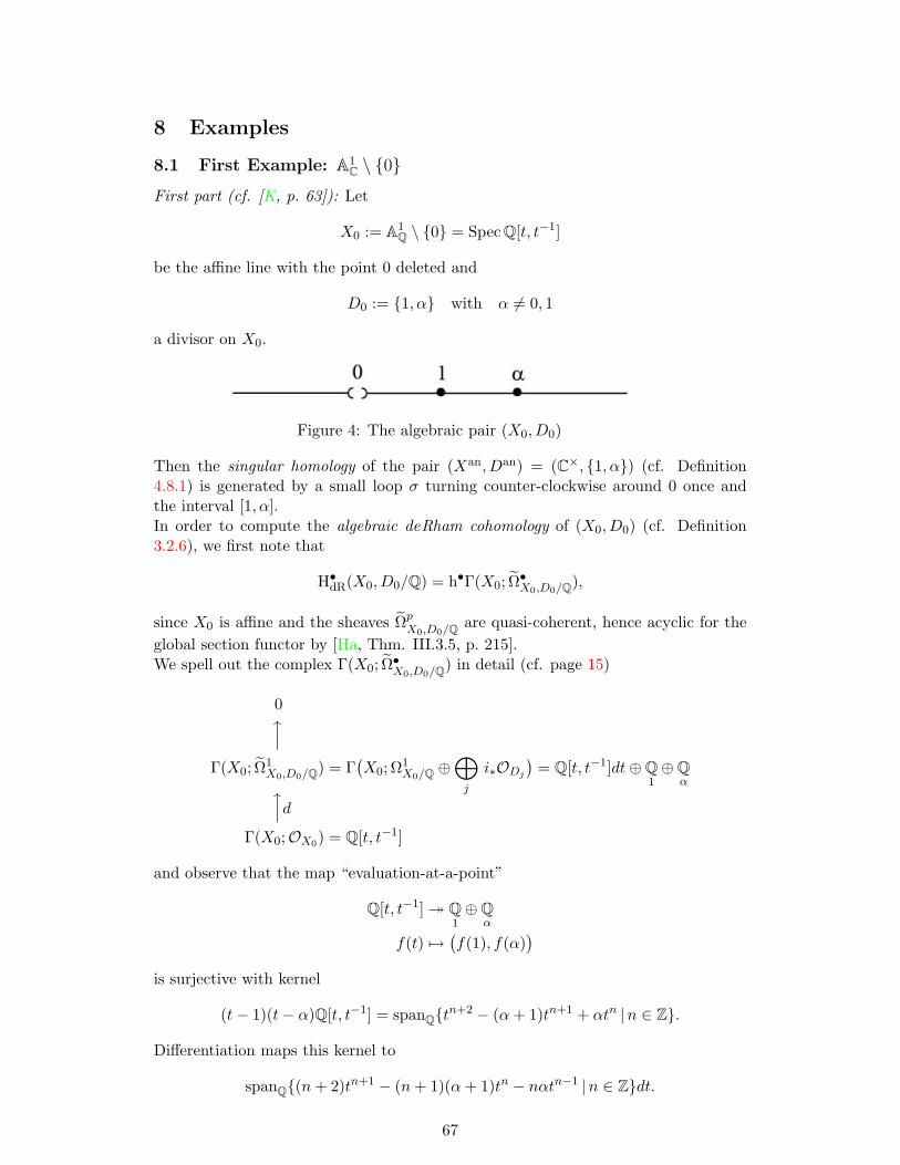
8 Examples

8.1 First Example: A1C \ 0

First part (cf. [K, p. 63]): Let

X0 := A1Q \ 0 = Spec Q[t, t−1]

be the affine line with the point 0 deleted and

D0 := 1, α with α 6= 0, 1

a divisor on X0.

Figure 4: The algebraic pair (X0, D0)

Then the singular homology of the pair (Xan, Dan) = (C×, 1, α) (cf. Definition4.8.1) is generated by a small loop σ turning counter-clockwise around 0 once andthe interval [1, α].In order to compute the algebraic deRham cohomology of (X0, D0) (cf. Definition3.2.6), we first note that

H•dR(X0, D0/Q) = h•Γ(X0; Ω•X0,D0/Q),

since X0 is affine and the sheaves ΩpX0,D0/Q are quasi-coherent, hence acyclic for the

global section functor by [Ha, Thm. III.3.5, p. 215].We spell out the complex Γ(X0; Ω•X0,D0/Q) in detail (cf. page 15)

0xΓ(X0; Ω1

X0,D0/Q) = Γ(X0; Ω1

X0/Q ⊕⊕j

i∗ODj

)= Q[t, t−1]dt⊕Q

1⊕Q

αxdΓ(X0;OX0) = Q[t, t−1]

and observe that the map “evaluation-at-a-point”

Q[t, t−1] Q1⊕Q

α

f(t) 7→(f(1), f(α)

)is surjective with kernel

(t− 1)(t− α)Q[t, t−1] = spanQtn+2 − (α+ 1)tn+1 + αtn |n ∈ Z.

Differentiation maps this kernel to

spanQ(n+ 2)tn+1 − (n+ 1)(α+ 1)tn − nαtn−1 |n ∈ Zdt.

67

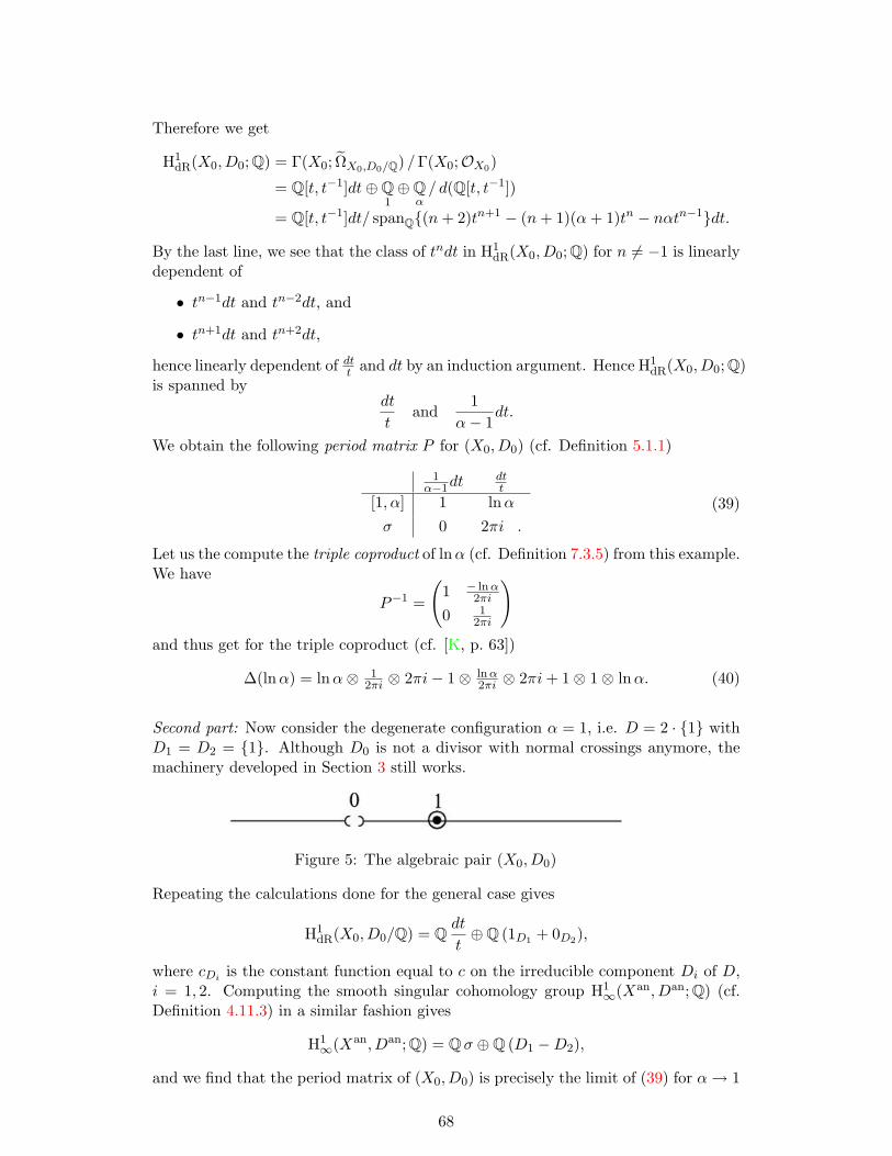
Therefore we get

H1dR(X0, D0; Q) = Γ(X0; ΩX0,D0/Q) /Γ(X0;OX0)

= Q[t, t−1]dt⊕Q1⊕Q

α/ d(Q[t, t−1])

= Q[t, t−1]dt/ spanQ(n+ 2)tn+1 − (n+ 1)(α+ 1)tn − nαtn−1dt.

By the last line, we see that the class of tndt in H1dR(X0, D0; Q) for n 6= −1 is linearly

dependent of

• tn−1dt and tn−2dt, and

• tn+1dt and tn+2dt,

hence linearly dependent of dtt and dt by an induction argument. Hence H1dR(X0, D0; Q)

is spanned bydt

tand

1α− 1

dt.

We obtain the following period matrix P for (X0, D0) (cf. Definition 5.1.1)

1α−1dt

dtt

[1, α] 1 lnασ 0 2πi .

(39)

Let us the compute the triple coproduct of lnα (cf. Definition 7.3.5) from this example.We have

P−1 =

(1 − lnα

2πi

0 12πi

)and thus get for the triple coproduct (cf. [K, p. 63])

∆(lnα) = lnα⊗ 12πi ⊗ 2πi− 1⊗ lnα

2πi ⊗ 2πi+ 1⊗ 1⊗ lnα. (40)

Second part: Now consider the degenerate configuration α = 1, i.e. D = 2 · 1 withD1 = D2 = 1. Although D0 is not a divisor with normal crossings anymore, themachinery developed in Section 3 still works.

Figure 5: The algebraic pair (X0, D0)

Repeating the calculations done for the general case gives

H1dR(X0, D0/Q) = Q

dt

t⊕Q (1D1 + 0D2),

where cDi is the constant function equal to c on the irreducible component Di of D,i = 1, 2. Computing the smooth singular cohomology group H1

∞(Xan, Dan; Q) (cf.Definition 4.11.3) in a similar fashion gives

H1∞(Xan, Dan; Q) = Qσ ⊕Q (D1 −D2),

and we find that the period matrix of (X0, D0) is precisely the limit of (39) for α→ 1

68

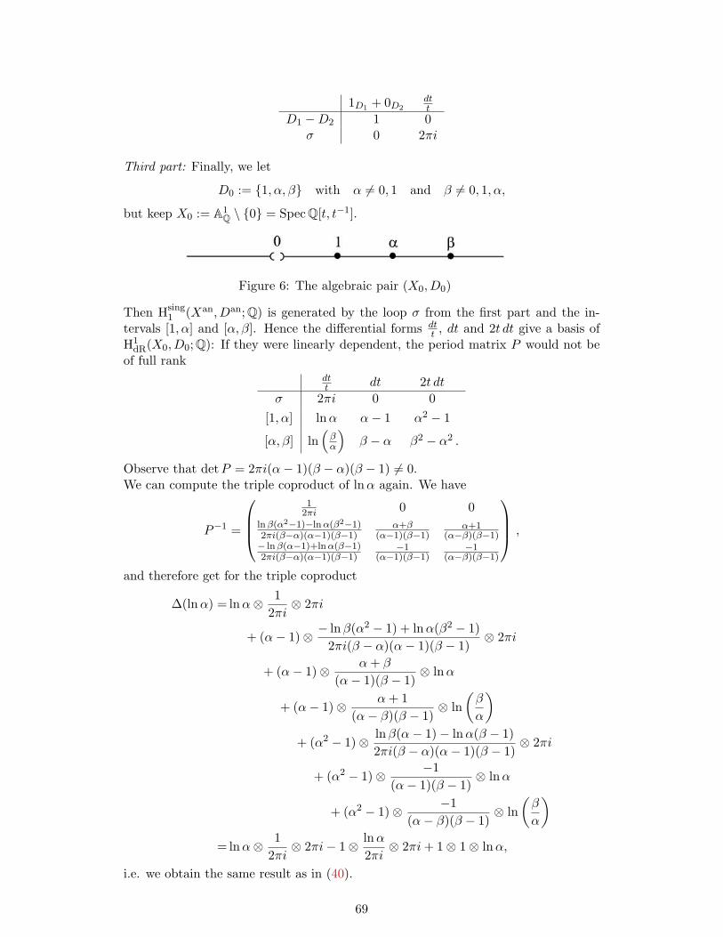
1D1 + 0D2dtt

D1 −D2 1 0σ 0 2πi

Third part: Finally, we let

D0 := 1, α, β with α 6= 0, 1 and β 6= 0, 1, α,

but keep X0 := A1Q \ 0 = Spec Q[t, t−1].

Figure 6: The algebraic pair (X0, D0)

Then Hsing1 (Xan, Dan; Q) is generated by the loop σ from the first part and the in-

tervals [1, α] and [α, β]. Hence the differential forms dtt , dt and 2t dt give a basis of

H1dR(X0, D0; Q): If they were linearly dependent, the period matrix P would not be

of full rankdtt dt 2t dt

σ 2πi 0 0[1, α] lnα α− 1 α2 − 1

[α, β] ln(βα

)β − α β2 − α2 .

Observe that detP = 2πi(α− 1)(β − α)(β − 1) 6= 0.We can compute the triple coproduct of lnα again. We have

P−1 =

1

2πi 0 0lnβ(α2−1)−lnα(β2−1)2πi(β−α)(α−1)(β−1)

α+β(α−1)(β−1)

α+1(α−β)(β−1)

− lnβ(α−1)+lnα(β−1)2πi(β−α)(α−1)(β−1)

−1(α−1)(β−1)

−1(α−β)(β−1)

,

and therefore get for the triple coproduct

∆(lnα) = lnα⊗ 12πi⊗ 2πi

+ (α− 1)⊗ − lnβ(α2 − 1) + lnα(β2 − 1)2πi(β − α)(α− 1)(β − 1)

⊗ 2πi

+ (α− 1)⊗ α+ β

(α− 1)(β − 1)⊗ lnα

+ (α− 1)⊗ α+ 1(α− β)(β − 1)

⊗ ln(β

α

)+ (α2 − 1)⊗ lnβ(α− 1)− lnα(β − 1)

2πi(β − α)(α− 1)(β − 1)⊗ 2πi

+ (α2 − 1)⊗ −1(α− 1)(β − 1)

⊗ lnα

+ (α2 − 1)⊗ −1(α− β)(β − 1)

⊗ ln(β

α

)= lnα⊗ 1

2πi⊗ 2πi− 1⊗ lnα

2πi⊗ 2πi+ 1⊗ 1⊗ lnα,

i.e. we obtain the same result as in (40).

69

8.2 Second Example: Quadratic Forms

LetQ(x) : Q3 −→ Q

x = (x0, x1, x2) 7→ xAxT

be a quadratic form with A ∈ Q3×3 being a regular, symmetric matrix.The zero-locus of Q(x)

X0 := x ∈ QP 2 |Q(x) = 0is a quadric or non-degenerate conic. We are interested in its affine piece

X0 := X0 ∩ x0 6= 0 ⊂ Q2 ⊂ QP 2.

We show that we can assume Q(x) to be of a particular nice form. A vector v ∈ Q3

is called Q-anisotropic, if Q(v) 6= 0. Since char Q 6= 2, there exist such vectors; justsuppose the contrary:

Q(1, 0, 0) = 0 gives A11 = 0,Q(0, 1, 0) = 0 gives A22 = 0,Q(1, 1, 0) = 0 gives 2 ·A12 = 0

and A would be degenerate. In particular

Q(1, λ, 0) = Q(1, 0, 0) + 2λQ(1, 1, 0) + λ2Q(0, 1, 0)

will be different form zero for almost all λ ∈ Q. Hence, we can assume that (1, 0, 0)is anisotropic after applying a coordinate transformation of the form

x′0 := x0, x′1 := −λx0 + x1, x′2 := x2.

After another affine change of coordinates, we can also assume that A is a diagonalmatrix by [Se, Ch. IV, § 1, 2, Thm. 1, p. 30]. An inspection of the proof of this resultreveals that we can choose this coordinate transformation such that the x0-coordinateis left unaltered. (Just take for e1 the anisotropic vector (1, 0, 0) in the proof.) Sucha transformation does not change the isomorphy-type of X0, and we can take X0 tobe cut out by an equation of the form

ax2 + by2 = 1 for a, b ∈ Q×

with affine coordinates x := x1x0

and y := x2x0

.Since X0 is affine, and hence the sheaves Ωp

X0/Q are Γ(X0; ?)-acyclic by [Ha, Thm.III.3.5, p. 215], we can compute its algebraic deRham cohomology (cf. Definition3.2.3) by

H•dR(X0/Q) = h•Γ(X0; Ω•X0/Q);

so we write down the complex Γ(X0; Ω•X0/Q) in detail

0↑

Γ(X0; Ω1X0/Q) = Q[x, y]/(ax2 + by2 − 1)dx, dy / (axdx+ bydy)

d ↑Γ(X0;OX0) = Q[x, y]/(ax2 + by2 − 1).

Obviously, H1dR(X0/Q) can be presented with generators xnymdx and xnymdy for

m,n ∈ N0 modulo numerous relations. We easily get

70

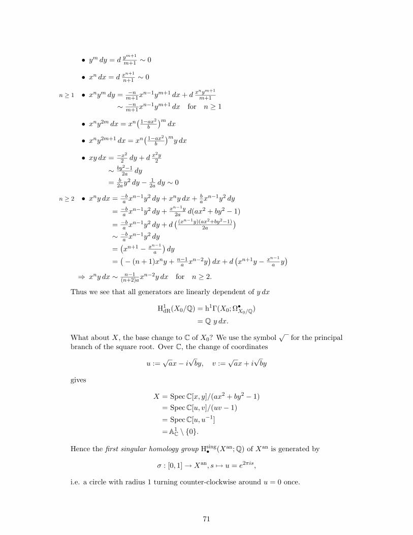
• ym dy = d ym+1

m+1 ∼ 0

• xn dx = d xn+1

n+1 ∼ 0

n ≥ 1 • xnym dy = −nm+1x

n−1ym+1 dx+ d xnym+1

m+1

∼ −nm+1x

n−1ym+1 dx for n ≥ 1

• xny2m dx = xn(

1−ax2

b

)mdx

• xny2m+1 dx = xn(

1−ax2

b

)my dx

• xy dx = −x2

2 dy + d x2y2

∼ by2−12a dy

= b2ay

2 dy − 12a dy ∼ 0

n ≥ 2 • xny dx = −ba x

n−1y2 dy + xny dx+ bax

n−1y2 dy

= −ba x

n−1y2 dy + xn−1y2a d(ax2 + by2 − 1)

= −ba x

n−1y2 dy + d( (xn−1y)(ax2+by2−1)

2a

)∼ −ba x

n−1y2 dy

=(xn+1 − xn−1

a

)dy

=(− (n+ 1)xny + n−1

a xn−2y)dx+ d

(xn+1y − xn−1

a y)

⇒ xny dx ∼ n−1(n+2)ax

n−2y dx for n ≥ 2.

Thus we see that all generators are linearly dependent of y dx

H1dR(X0/Q) = h1Γ(X0; Ω•X0/Q)

= Q y dx.

What about X, the base change to C of X0? We use the symbol√

for the principalbranch of the square root. Over C, the change of coordinates

u :=√ax− i

√by, v :=

√ax+ i

√by

gives

X = Spec C[x, y]/(ax2 + by2 − 1)= Spec C[u, v]/(uv − 1)

= Spec C[u, u−1]

= A1C \ 0.

Hence the first singular homology group Hsing• (Xan; Q) of Xan is generated by

σ : [0, 1]→ Xan, s 7→ u = e2πis,

i.e. a circle with radius 1 turning counter-clockwise around u = 0 once.

71

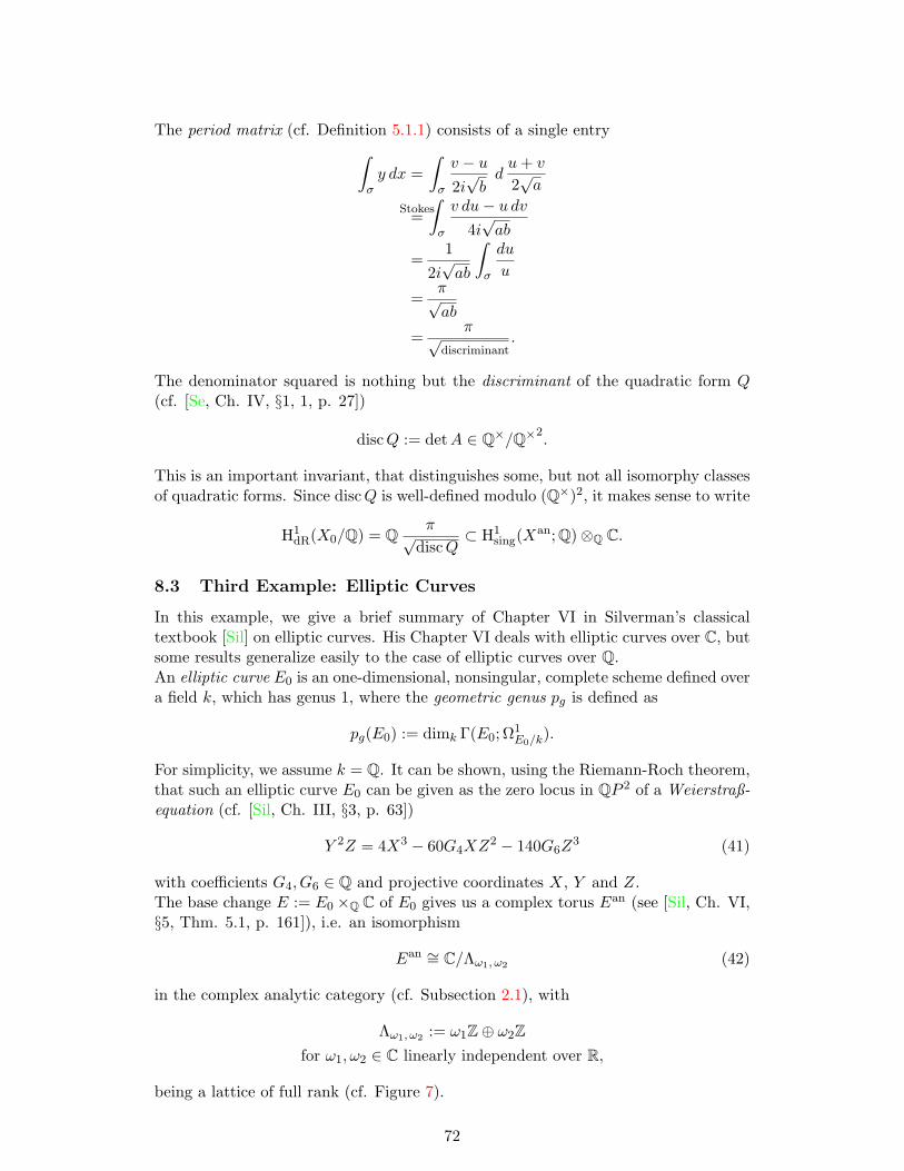
The period matrix (cf. Definition 5.1.1) consists of a single entry∫σy dx =

∫σ

v − u2i√bdu+ v

2√a

Stokes=∫σ

v du− u dv4i√ab

=1

2i√ab

∫σ

du

u

=π√ab

=π√

discriminant.

The denominator squared is nothing but the discriminant of the quadratic form Q(cf. [Se, Ch. IV, §1, 1, p. 27])

discQ := detA ∈ Q×/Q×2.

This is an important invariant, that distinguishes some, but not all isomorphy classesof quadratic forms. Since discQ is well-defined modulo (Q×)2, it makes sense to write

H1dR(X0/Q) = Q

π√discQ

⊂ H1sing(X

an; Q)⊗Q C.

8.3 Third Example: Elliptic Curves

In this example, we give a brief summary of Chapter VI in Silverman’s classicaltextbook [Sil] on elliptic curves. His Chapter VI deals with elliptic curves over C, butsome results generalize easily to the case of elliptic curves over Q.An elliptic curve E0 is an one-dimensional, nonsingular, complete scheme defined overa field k, which has genus 1, where the geometric genus pg is defined as

pg(E0) := dimk Γ(E0; Ω1E0/k

).

For simplicity, we assume k = Q. It can be shown, using the Riemann-Roch theorem,that such an elliptic curve E0 can be given as the zero locus in QP 2 of a Weierstraß-equation (cf. [Sil, Ch. III, §3, p. 63])

Y 2Z = 4X3 − 60G4XZ2 − 140G6Z

3 (41)

with coefficients G4, G6 ∈ Q and projective coordinates X, Y and Z.The base change E := E0 ×Q C of E0 gives us a complex torus Ean (see [Sil, Ch. VI,§5, Thm. 5.1, p. 161]), i.e. an isomorphism

Ean ∼= C/Λω1, ω2 (42)

in the complex analytic category (cf. Subsection 2.1), with

Λω1, ω2 := ω1Z⊕ ω2Zfor ω1, ω2 ∈ C linearly independent over R,

being a lattice of full rank (cf. Figure 7).

72

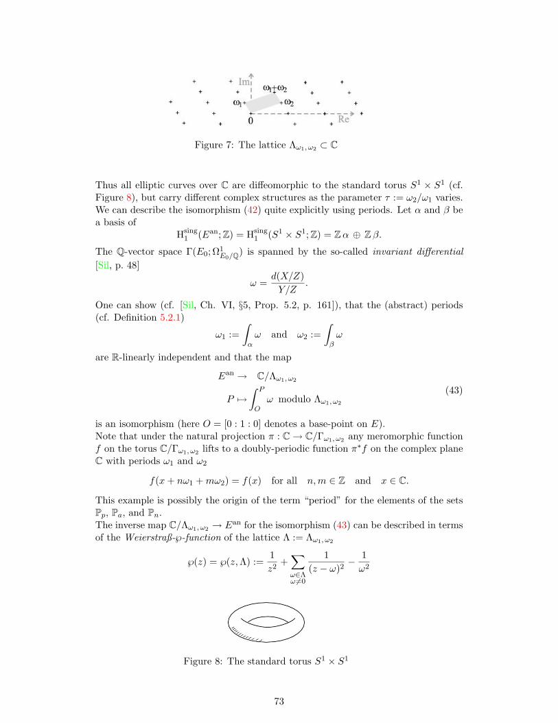
Figure 7: The lattice Λω1, ω2 ⊂ C

Thus all elliptic curves over C are diffeomorphic to the standard torus S1 × S1 (cf.Figure 8), but carry different complex structures as the parameter τ := ω2/ω1 varies.We can describe the isomorphism (42) quite explicitly using periods. Let α and β bea basis of

Hsing1 (Ean; Z) = Hsing

1 (S1 × S1; Z) = Zα ⊕ Zβ.

The Q-vector space Γ(E0; Ω1E0/Q) is spanned by the so-called invariant differential

[Sil, p. 48]

ω =d(X/Z)Y/Z

.

One can show (cf. [Sil, Ch. VI, §5, Prop. 5.2, p. 161]), that the (abstract) periods(cf. Definition 5.2.1)

ω1 :=∫αω and ω2 :=

∫βω

are R-linearly independent and that the map

Ean → C/Λω1, ω2

P 7→∫ P

Oω modulo Λω1, ω2

(43)

is an isomorphism (here O = [0 : 1 : 0] denotes a base-point on E).Note that under the natural projection π : C→ C/Γω1, ω2 any meromorphic functionf on the torus C/Γω1, ω2 lifts to a doubly-periodic function π∗f on the complex planeC with periods ω1 and ω2

f(x+ nω1 +mω2) = f(x) for all n,m ∈ Z and x ∈ C.

This example is possibly the origin of the term “period” for the elements of the setsPp, Pa, and Pn.The inverse map C/Λω1, ω2 → Ean for the isomorphism (43) can be described in termsof the Weierstraß-℘-function of the lattice Λ := Λω1, ω2

℘(z) = ℘(z,Λ) :=1z2

+∑ω∈Λω 6=0

1(z − ω)2

− 1ω2

Figure 8: The standard torus S1 × S1

73

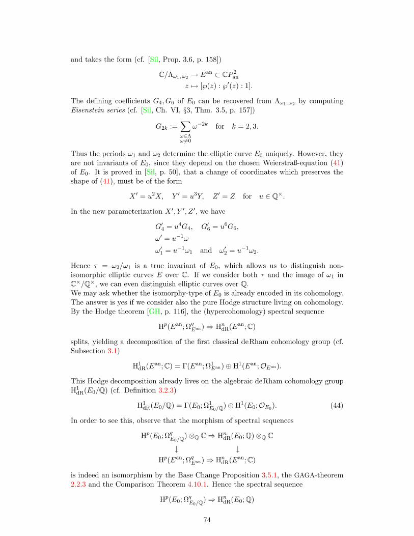
and takes the form (cf. [Sil, Prop. 3.6, p. 158])

C/Λω1, ω2 → Ean ⊂ CP 2an

z 7→ [℘(z) : ℘′(z) : 1].

The defining coefficients G4, G6 of E0 can be recovered from Λω1, ω2 by computingEisenstein series (cf. [Sil, Ch. VI, §3, Thm. 3.5, p. 157])

G2k :=∑ω∈Λω 6=0

ω−2k for k = 2, 3.

Thus the periods ω1 and ω2 determine the elliptic curve E0 uniquely. However, theyare not invariants of E0, since they depend on the chosen Weierstraß-equation (41)of E0. It is proved in [Sil, p. 50], that a change of coordinates which preserves theshape of (41), must be of the form

X ′ = u2X, Y ′ = u3Y, Z ′ = Z for u ∈ Q×.

In the new parameterization X ′, Y ′, Z ′, we have

G′4 = u4G4, G′6 = u6G6,

ω′ = u−1ω

ω′1 = u−1ω1 and ω′2 = u−1ω2.

Hence τ = ω2/ω1 is a true invariant of E0, which allows us to distinguish non-isomorphic elliptic curves E over C. If we consider both τ and the image of ω1 inC×/Q×, we can even distinguish elliptic curves over Q.We may ask whether the isomorphy-type of E0 is already encoded in its cohomology.The answer is yes if we consider also the pure Hodge structure living on cohomology.By the Hodge theorem [GH, p. 116], the (hypercohomology) spectral sequence

Hp(Ean; ΩqEan)⇒ Hn

dR(Ean; C)

splits, yielding a decomposition of the first classical deRham cohomology group (cf.Subsection 3.1)

H1dR(Ean; C) = Γ(Ean; Ω1

Ean)⊕H1(Ean;OEan).

This Hodge decomposition already lives on the algebraic deRham cohomology groupH1

dR(E0/Q) (cf. Definition 3.2.3)

H1dR(E0/Q) = Γ(E0; Ω1

E0/Q)⊕H1(E0;OE0). (44)

In order to see this, observe that the morphism of spectral sequences

Hp(E0; ΩqE0/Q)⊗Q C⇒ Hn

dR(E0; Q)⊗Q C

↓ ↓Hp(Ean; Ωq

Ean)⇒ HndR(Ean; C)

is indeed an isomorphism by the Base Change Proposition 3.5.1, the GAGA-theorem2.2.3 and the Comparison Theorem 4.10.1. Hence the spectral sequence

Hp(E0; ΩqE0/Q)⇒ Hn

dR(E0; Q)

74

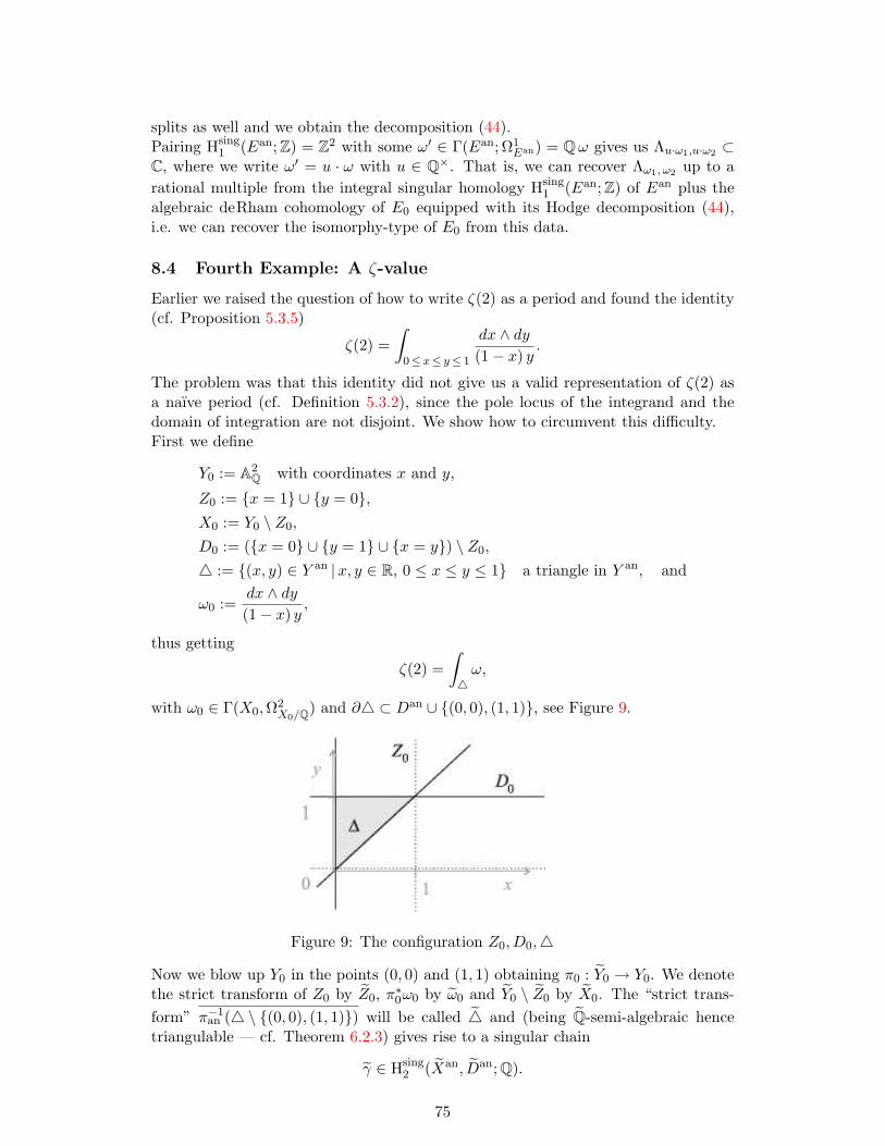
splits as well and we obtain the decomposition (44).Pairing Hsing

1 (Ean; Z) = Z2 with some ω′ ∈ Γ(Ean; Ω1Ean) = Qω gives us Λu·ω1,u·ω2 ⊂

C, where we write ω′ = u · ω with u ∈ Q×. That is, we can recover Λω1, ω2 up to arational multiple from the integral singular homology Hsing

1 (Ean; Z) of Ean plus thealgebraic deRham cohomology of E0 equipped with its Hodge decomposition (44),i.e. we can recover the isomorphy-type of E0 from this data.

8.4 Fourth Example: A ζ-value

Earlier we raised the question of how to write ζ(2) as a period and found the identity(cf. Proposition 5.3.5)

ζ(2) =∫

0≤x≤ y≤ 1

dx ∧ dy(1− x) y

.

The problem was that this identity did not give us a valid representation of ζ(2) asa naıve period (cf. Definition 5.3.2), since the pole locus of the integrand and thedomain of integration are not disjoint. We show how to circumvent this difficulty.First we define

Y0 := A2Q with coordinates x and y,

Z0 := x = 1 ∪ y = 0,X0 := Y0 \ Z0,

D0 := (x = 0 ∪ y = 1 ∪ x = y) \ Z0,

4 := (x, y) ∈ Y an |x, y ∈ R, 0 ≤ x ≤ y ≤ 1 a triangle in Y an, and

ω0 :=dx ∧ dy(1− x) y

,

thus getting

ζ(2) =∫4ω,

with ω0 ∈ Γ(X0,Ω2X0/Q) and ∂4 ⊂ Dan ∪ (0, 0), (1, 1), see Figure 9.

Figure 9: The configuration Z0, D0,4

Now we blow up Y0 in the points (0, 0) and (1, 1) obtaining π0 : Y0 → Y0. We denotethe strict transform of Z0 by Z0, π∗0ω0 by ω0 and Y0 \ Z0 by X0. The “strict trans-form” π−1

an (4 \ (0, 0), (1, 1)) will be called 4 and (being Q-semi-algebraic hencetriangulable — cf. Theorem 6.2.3) gives rise to a singular chain

γ ∈ Hsing2 (Xan, Dan; Q).

75

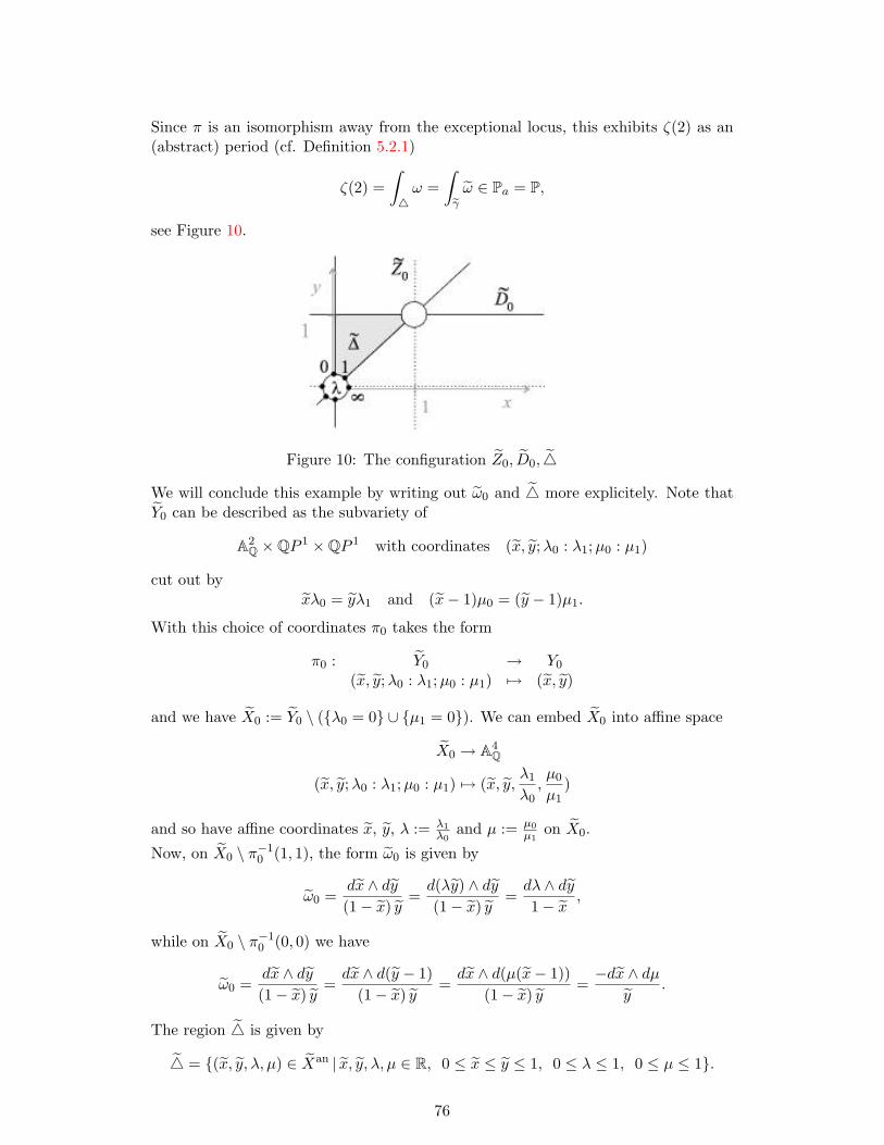
Since π is an isomorphism away from the exceptional locus, this exhibits ζ(2) as an(abstract) period (cf. Definition 5.2.1)

ζ(2) =∫4ω =

∫eγ ω ∈ Pa = P,

see Figure 10.

Figure 10: The configuration Z0, D0, 4

We will conclude this example by writing out ω0 and 4 more explicitely. Note thatY0 can be described as the subvariety of

A2Q ×QP 1 ×QP 1 with coordinates (x, y;λ0 : λ1;µ0 : µ1)

cut out byxλ0 = yλ1 and (x− 1)µ0 = (y − 1)µ1.

With this choice of coordinates π0 takes the form

π0 : Y0 → Y0

(x, y;λ0 : λ1;µ0 : µ1) 7→ (x, y)

and we have X0 := Y0 \ (λ0 = 0 ∪ µ1 = 0). We can embed X0 into affine space

X0 → A4Q

(x, y;λ0 : λ1;µ0 : µ1) 7→ (x, y,λ1

λ0,µ0

µ1)

and so have affine coordinates x, y, λ := λ1λ0

and µ := µ0

µ1on X0.

Now, on X0 \ π−10 (1, 1), the form ω0 is given by

ω0 =dx ∧ dy(1− x) y

=d(λy) ∧ dy(1− x) y

=dλ ∧ dy1− x

,

while on X0 \ π−10 (0, 0) we have

ω0 =dx ∧ dy(1− x) y

=dx ∧ d(y − 1)

(1− x) y=dx ∧ d(µ(x− 1))

(1− x) y=−dx ∧ dµ

y.

The region 4 is given by

4 = (x, y, λ, µ) ∈ Xan | x, y, λ, µ ∈ R, 0 ≤ x ≤ y ≤ 1, 0 ≤ λ ≤ 1, 0 ≤ µ ≤ 1.

76

8.5 Fifth Example: The Double Logarithm Variation of Mixed HodgeStructures

The previous example fits into a more general framework.

8.5.1 Multiple Polylogarithms

Define the hyperlogarithm as the iterated integral

In(a1, . . . , an) :=∫

0≤t1≤···≤tn≤1

dt1t1 − a1

∧ · · · ∧ dtntn − an

with a1, . . . , an ∈ C (cf. [Z1, p. 168]). These integrals specialize to the multiplepolylogarithm (cf. [loc. cit.]1)

Lim1,...,mn

(a2

a1, · · · , an

an−1,

1an

):= (−1)n IP

mn(a1, 0, . . . , 0︸ ︷︷ ︸

m1−1

, . . . , an, 0, . . . , 0︸ ︷︷ ︸mn−1

),

which is convergent if 1 < |a1| < · · · < |an| (cf. [G3, 2.3, p. 9]). Alternatively, we candescribe the multiple polylogarithm as a power series (cf. [G3, Thm. 2.2, p. 9])

Lim1,...,mn(x1, . . . , xn) =∑

0<k1<···<kn

xk11 · · ·xknn

km11 · · · k

mnn

for |xi| < 1. (45)

Of special interest to us will be the dilogarithm Li2(x) =∑

k>0xk

k2 and the double

logarithm Li1,1(x, y) =∑

0<k<lxkyl

kl .At first, the functions Lim1,...,mn(x1, . . . , xn) only make sense for |xi| < 1, but theycan be analytically continued to multivalued meromorphic functions on Cn (cf. [Z1,p. 2]), for example Li1(x) = − ln(1− x).

General Remarks. Polylogarithms have applications in Zagier’s conjecture (cf.[Z1, p. 2]) and are used in the study of certain motivic fundamental groups (cf. [HW,p. 9] and [G2]).Besides, equation (45) would suggest a connection between values of multiple poly-logarithms and multiple ζ-values (cf. [G1, p. 617])

ζ(m1, . . . ,mn) :=∑

0<k1<...<km

1km1

1 · · · kmnn

.

Indeed, we have formally

−ζ(2) =−π2

6= −Li2(1) = lim

b→0lima→1

I2(a, b) = limb→0

lima→1

Li1,1

(b

a,1b

).

However, such formal computations are problematic, since a limit may diverge or atleast depend on the direction in which the limit is taken, because multiple polylog-arithms are multivalued. To deal with this problem, Zagier, Goncharov and othersproposed regularization procedures, for which we have to refer to [G3, 2.9–2.10, p. 18–24].

1Note that the factor (−1)n is missing in equation (1.2) of [Z1, p. 168].

77

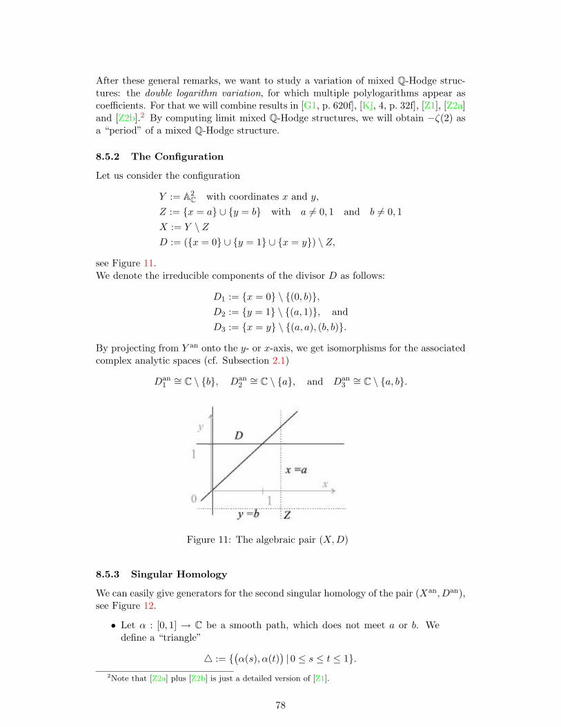
After these general remarks, we want to study a variation of mixed Q-Hodge struc-tures: the double logarithm variation, for which multiple polylogarithms appear ascoefficients. For that we will combine results in [G1, p. 620f], [Kj, 4, p. 32f], [Z1], [Z2a]and [Z2b].2 By computing limit mixed Q-Hodge structures, we will obtain −ζ(2) asa “period” of a mixed Q-Hodge structure.

8.5.2 The Configuration

Let us consider the configuration

Y := A2C with coordinates x and y,

Z := x = a ∪ y = b with a 6= 0, 1 and b 6= 0, 1X := Y \ ZD := (x = 0 ∪ y = 1 ∪ x = y) \ Z,

see Figure 11.We denote the irreducible components of the divisor D as follows:

D1 := x = 0 \ (0, b),D2 := y = 1 \ (a, 1), andD3 := x = y \ (a, a), (b, b).

By projecting from Y an onto the y- or x-axis, we get isomorphisms for the associatedcomplex analytic spaces (cf. Subsection 2.1)

Dan1∼= C \ b, Dan

2∼= C \ a, and Dan

3∼= C \ a, b.

Figure 11: The algebraic pair (X,D)

8.5.3 Singular Homology

We can easily give generators for the second singular homology of the pair (Xan, Dan),see Figure 12.

• Let α : [0, 1] → C be a smooth path, which does not meet a or b. Wedefine a “triangle”

4 := (α(s), α(t)

)| 0 ≤ s ≤ t ≤ 1.

2Note that [Z2a] plus [Z2b] is just a detailed version of [Z1].

78

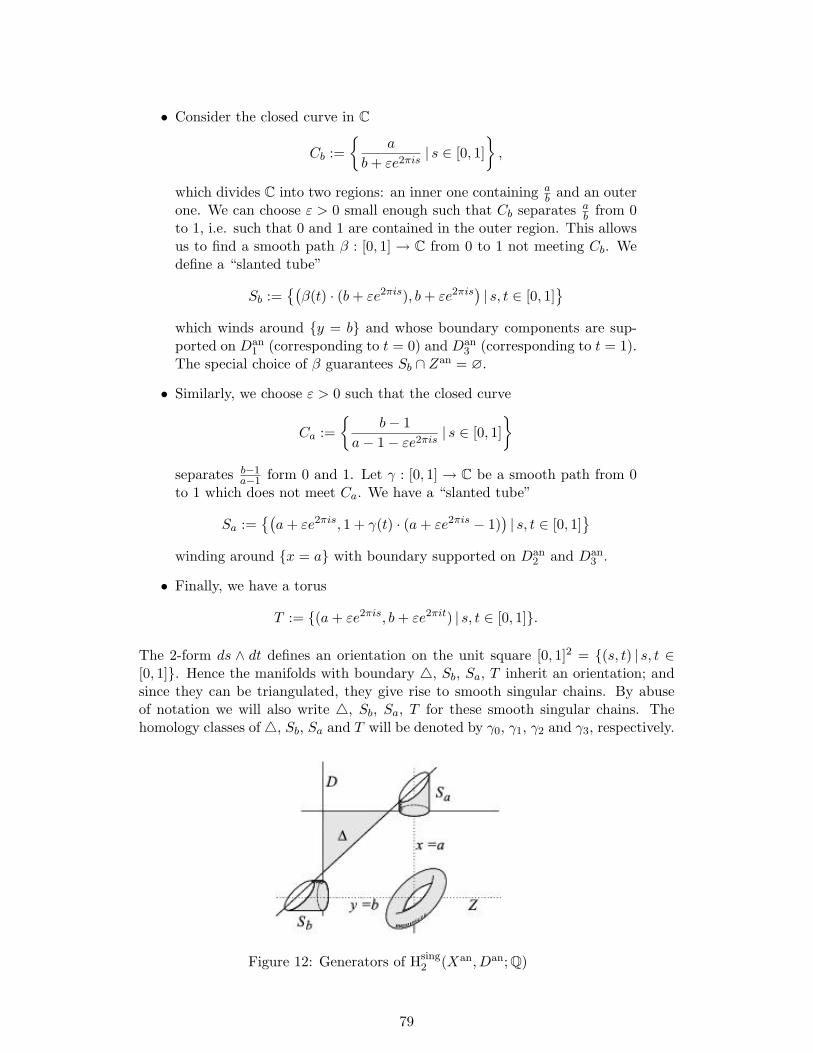
• Consider the closed curve in C

Cb :=

a

b+ εe2πis| s ∈ [0, 1]

,

which divides C into two regions: an inner one containing ab and an outer

one. We can choose ε > 0 small enough such that Cb separates ab from 0

to 1, i.e. such that 0 and 1 are contained in the outer region. This allowsus to find a smooth path β : [0, 1] → C from 0 to 1 not meeting Cb. Wedefine a “slanted tube”

Sb :=(β(t) · (b+ εe2πis), b+ εe2πis

)| s, t ∈ [0, 1]

which winds around y = b and whose boundary components are sup-ported on Dan

1 (corresponding to t = 0) and Dan3 (corresponding to t = 1).

The special choice of β guarantees Sb ∩ Zan = ∅.

• Similarly, we choose ε > 0 such that the closed curve

Ca :=

b− 1a− 1− εe2πis

| s ∈ [0, 1]

separates b−1a−1 form 0 and 1. Let γ : [0, 1] → C be a smooth path from 0

to 1 which does not meet Ca. We have a “slanted tube”

Sa :=(a+ εe2πis, 1 + γ(t) · (a+ εe2πis − 1)

)| s, t ∈ [0, 1]

winding around x = a with boundary supported on Dan

2 and Dan3 .

• Finally, we have a torus

T := (a+ εe2πis, b+ εe2πit) | s, t ∈ [0, 1].

The 2-form ds ∧ dt defines an orientation on the unit square [0, 1]2 = (s, t) | s, t ∈[0, 1]. Hence the manifolds with boundary 4, Sb, Sa, T inherit an orientation; andsince they can be triangulated, they give rise to smooth singular chains. By abuseof notation we will also write 4, Sb, Sa, T for these smooth singular chains. Thehomology classes of4, Sb, Sa and T will be denoted by γ0, γ1, γ2 and γ3, respectively.

Figure 12: Generators of Hsing2 (Xan, Dan; Q)

79

An inspection of the long exact sequence in singular homology will reveal that γ0, . . . , γ3

form a system generators (see the following proof)

Hsing2 (Dan; Q) −−−−→ Hsing

2 (Xan; Q) −−−−→ Hsing2 (Xan, Dan; Q) −−−−→

Hsing1 (Dan; Q) i1−−−−→ Hsing

1 (Xan; Q) .

Claim 8.5.1. With notation as above, we have for the second singular homology ofthe pair (Xan, Dan)

Hsing2 (Xan, Dan; Q) = Q γ0 ⊕Q γ1 ⊕Q γ2 ⊕Q γ3.

Proof. For c := a and c := b, the inclusion of the circle c + εe2πis | s ∈ [0, 1] intoC\c is a homotopy equivalence, hence the product map T → Xan is also a homotopyequivalence. This shows

Hsing2 (Xan; Q) = QT,

while Hsing1 (Xan; Q) has rank two with generators

• one loop winding counterclockwise around x = a once, but not aroundy = b, thus being homologous to both ∂Sa ∩Dan

2 and −∂Sa ∩Dan3 , and

• another loop winding counterclockwise around y = b once, but notaround x = a, thus being homologous to ∂Sb ∩Dan

1 and −∂Sb ∩Dan3 .

In order to compute the Betti-numbers bi of Dan, we use the spectral sequence fromProposition 4.4.2 for the closed covering Dan

i

Ep,q2 :=

· · · 0 0 0 0 · · ·· · · 0

⊕3i=1 H1

dR(Dani ; C) 0 0 · · ·

· · · 0 ker δ coker δ 0 · · ·· · · 0 0 0 0 · · ·

⇒ En∞ := HndR(Dan; C),

where

δ :3⊕i=1

H0dR(Dan

i ; C) −→⊕i<j

H0dR(Dan

ij ; C).

Note that this spectral sequence degenerates. Since Dan is connected, we have b0 = 1,i.e.

1 = b0 = rankCE0∞ = rankCE

0,02 = rankC ker δ.

Hence

rankC coker δ = rankC codomain δ − rankC domain δ + rankC ker δ= (1 + 1 + 1)− (1 + 1 + 1) + 1 = 1,

and so

b1 = rankCE1∞ = rankCE

1,02 + rankCE

0,12

=3∑i=1

rankC H1dR(Dan

i ; C) + rankC coker δ

= rankC H1(C \ b; C) + rankC H1(C \ a; C) + rankC H1(C \ a, b; C) + 1= (1 + 1 + 2) + 1 = 5.

80

We can easily specify generators of Hsing1 (Dan; Q) as follows

Hsing1 (Dan; Q) = Q·(∂Sb∩Dan

1 )⊕Q·(∂Sa∩Dan2 )⊕Q·(∂Sb∩Dan

3 )⊕Q·(∂Sa∩Dan3 )⊕Q·∂4.

Clearly b2 = rankC Hsing2 (Dan; Q) = 0. Now we can compute ker i1 and obtain

ker i1 = Q · ∂4⊕Q · (∂Sb ∩Dan1 + ∂Sb ∩Dan

3 )⊕Q · (∂Sa ∩Dan2 + ∂Sa ∩Dan

3 ).

This shows finally

rankQ Hsing2 (Xan, Dan; Q) = rankQ Hsing

2 (Xan; Q) + rankQ ker i1 = 1 + 3 = 4.

From these explicit calculations we also derive the linear independence of γ0 = [4],γ1 = [Sb], γ2 = [Sa], γ3 = [T ] and Claim 8.5.1 is proved.

8.5.4 Smooth Singular Homology

Recall the definition of smooth singular cohomology (cf. Definition 4.11.3). With thevarious sign conventions made so far (cf. Subsection 4.11.1 and the appendix), theboundary map δ : C∞2 (Xan, Dan; Q)→ C∞1 (Xan, Dan; Q) is given by

δ : C∞2 (Xan; Q)⊕3⊕i=1

C∞1 (Dani ; Q)⊕

⊕i<j

C∞0 (Danij ; Q)→ C∞1 (Xan; Q)⊕

3⊕i=1

(Dani ; Q)

(σ∅, σ1

1, σ2

2, σ3

3, σ12

12, σ13

13, σ23

23) 7→

(∂σ + σ1 + σ2 + σ3∅

,−∂σ1 + σ12 + σ131

,−∂σ2 − σ12 + σ232

,−∂σ3 − σ13 − σ233

).

Thus the following elements of C∞2 (Xan, Dan; Q) are cycles

• Γ0 := (4∅,−∂4∩Dan

11

,−∂4∩Dan2

2,−∂4∩Dan

33

, Dan12

12,−Dan

1313

, Dan23

23),

• Γ1 := (Sb∅,−∂Sb ∩Dan

11

, 02,−∂Sb ∩Dan

33

, 012, 013, 023

),

• Γ2 := (Sa∅, 01,−∂Sa ∩Dan

22

, 03,−∂Sa ∩Dan

312

, 013, 023

) and

• Γ3 := (T∅, 01, 02, 03, 012, 013, 023

).

Under the isomorphism H∞2 (Xan, Dan; Q) ∼−→ Hsing2 (Xan, Dan; Q) the classes of these

cycles [Γ0], [Γ1], [Γ2], [Γ3] are mapped to γ0, γ1, γ2, γ3, respectively (cf. Proposition4.11.5).

8.5.5 Algebraic DeRham Cohomology of (Xan, Dan)

Recall the definition of the complex Ω•X,D/C on page 15. We consider

Γ(X; Ω2X,D/C) = Γ(X; Ω2

X/C)⊕3⊕i=1

Γ(Di; Ω1Di/C)⊕

⊕i<j

Γ(Dij ;ODij )

together with the following cycles of Γ(X; Ω2X,D/C)

81

• ω0 := ( dx∧dy(x−a)(y−b)

∅, 01, 02, 03, 012, 013, 023

),

• ω1 := (0∅, −dyy−b

1

, 02, 03, 012, 013, 023

),

• ω2 := (0∅, 01, −dxx−a

2

, 03, 012, 013, 023

), and

• ω3 := (0∅, 01, 02, 03, 012, 013, 123

).

By computing the (transposed) period matrix Pij := 〈Γj , ωi〉 (cf. Definition 5.1.1)and checking its non-degeneracy, we will show that ω0, . . ., ω3 span H2

dR(X,D/C).

Claim 8.5.2. Let X and D be as in Subsection 8.5.2. Then the second algebraic deRham cohomology group H2

dR(X,D/C) of the pair (X,D) is generated by the cyclesω0, . . . , ω3 considered above.

8.5.6 Period Matrix of (X,D)

Easy calculations give us for the (transposed) period matrix P := (〈Γj , ωi〉)3i,j=1 (cf.Definition 5.1.1)

Γ0 Γ1 Γ2 Γ3

ω0 1 0 0 0ω1 Li1(1

b ) 2πi 0 0ω2 Li1( 1

a) 0 2πi 0ω3 ? 2πiLi1( ba) 2πi ln

(a−b1−b

)(2πi)2;

for example (cf. Subsection 4.11.5)

• P1,1 = 〈Γ1, ω1〉 =∫−∂Sb∩Dan

1

−dyy−b

=∫|y−b|=ε

dyy−b

= 2πi,

• P3,3 = 〈Γ3, ω3〉 =∫T

dxx−a ∧

dyy−b

=(∫|x−a|=ε

dxx−a

)·(∫|y−b|=ε

dyy−b

)by Fubini

= (2πi)2,

• P1,0 = 〈Γ0, ω1〉 =∫−∂4∩Dan

1

−dyy−b

=∫ 10−α(t)α(t)−b

= −[ln(α(t))− b]10= − ln

(1−b−b

)= − ln

(1− 1

b

)= Li1

(1b

), and

• P3,1 = 〈Γ1, ω3〉 =∫Sb

dxx−a ∧

dyy−b

=∫[0,1]2

d(β(t)·(b+εe2πis))β(t)·(b+εe2πis)−a ∧

d(b+εe2πis)εe2πis

82

=∫[0,1]2

b+εe2πis

β(t)·(b+εe2πis)−adβ(t) ∧ 2πids

= −∫ 1

0

[a ln(β(t)·(b+εe2πis)−a)−2πiβ(t)bs

β(t)·(−β(t)b+a)

]1

0

dβ(t)

= −2πi∫ 10

dβ(t)β(t)−a

b

= −2πi[ln(β(t)− a

b

)]10

= −2πi ln(

1−ab

−ab

)= −2πi ln

(1− a

b

)= 2πiLi1

(ba

).

Obviously the period matrix P is non-degenerate and so Claim 8.5.2 is proved.What about the entry P3,0? We want to show that 〈Γ0, ω3〉 = Li1,1

(ba ,

1b

), where

Li1,1(x, y) is an analytic continuation of the double logarithm defined for |x|, |y| < 1in Subsection 8.5.1.

8.5.7 Analytic Continuation of the Double Logarithm Li1,1(x, y)

We describe this analytic continuation in detail. Our approach is similar to the onetaken in [G3, 2.3, p. 9], but differs from that in [Z2a, p. 7].Let Ban := (C \ 0, 1)2 be the parameter space and choose a point (a, b) ∈ Ban. Forε > 0 we denote by Dε(a, b) the polycylinder

Dε(a, b) := (a, b) ∈ Ban | |a′ − a| < ε, |b′ − b| < ε.

If α : [0, 1] → C is a smooth path from 0 to 1 passing through neither a nor b, thenthere exists an ε > 0 such that imα does not meet any of the discs

D2ε(a) := a′ ∈ C | |a′ − a| < 2ε, andD2ε(b) := b ′ ∈ C | |b ′ − b| < 2ε.

Hence the power series (46) below

1α(s)− a′

1α(t)− b ′

=1

α(s)− a1

1− a′−aα(s)−a

1α(t)− b

11− b ′−b

α(t)−b

=∞∑

k,l=0

1(α(s)− a)k+1(α(t)− b)l+1︸ ︷︷ ︸

ck.l

(a′ − a)k(b ′ − b)l (46)

has coefficients ck,l satisfying

|ck,l| <(

12ε

)k+l+2

.

In particular, (46) converges uniformly for (a′, b ′) ∈ Dε(a, b) and we see that theintegral

Iα2 (a′, b ′) :=∫

0≤s≤t≤1

dα(s)α(s)− a′

∧ dα(t)α(t)− b ′

=∑k,l=0

(∫0≤s≤t≤1

dα(s)(α(s)− a)k+1

∧ dα(t)(α(t)− b)l+1

)(a′ − a)k(b ′ − b)l

83

defines an analytic function of Dε(a, b). In fact, by the same argument we get ananalytic function Iα2 on all of (C \ imα)2.Now let αr : [0, 1] → C \ (D2ε(a) ∪D2ε(b)) with r ∈ [0, 1] be a smooth homotopy ofpaths from 0 to 1, i.e. αr(0) = 0 and αr(1) = 1 for all r ∈ [0, 1]. We show

Iα02 (a′, b ′) = Iα1

2 (a′, b ′) for all (a′, b ′) ∈ Dε(a, b).

Define a subset Γ ⊂ C2

Γ := (αr(s), αr(t)) | 0 ≤ s ≤ t ≤ 1, r ∈ [0, 1].

The boundary of Γ is built out of five components (each being a manifold with bound-ary)

• Γs=0 := (0, αr(t)) | r, t ∈ [0, 1],

• Γs=t := (αr(s), αr(s)) | r, s ∈ [0, 1],

• Γt=1 := (αr(s), 1) | r, s ∈ [0, 1],

• Γr=0 := (α0(s), α0(t) | 0 ≤ s ≤ t ≤ 1,

• Γr=1 := (α1(s), α1(t) | 0 ≤ s ≤ t ≤ 1.

Let (a′, b ′) ∈ Dε(a, b). Since the restriction of dxx−a′ ∧

dyy−b ′ to Γs=0, Γs=t and Γt=1 is

zero, we get by Stoke’s theorem

0 =∫

Γ0 =

∫Γd

dx

x− a′∧ dy

y − b ′

=∫∂Γ

dx

x− a′∧ dy

y − b ′

=∫

Γr=1−Γr=0

dx

x− a′dy

y − b ′

= Iα12 (a′, b ′)− Iα0

2 (a′, b ′).

For each pair of smooth paths α0, α1 : [0, 1]→ C from 0 to 1, we can find a homotopyαr relative to 0, 1 between both paths. Since imαr is compact, we also find a point(a, b) ∈ Ban = (C \ 0, 1)2 and an ε > 0 such that imαr does not meet D2ε(a, b)or D2ε(a, b). Then Iα0

2 and Iα12 must agree on Dε(a, b). By the identity principle

for analytic functions of several complex variables [Gun, A, 3, p. 5], the functionsIα2 (a′, b ′), each defined on (C \ imα)2, patch together to give a multivalued analyticfunction on Ban = (C \ 0, 1)2.Now assume 1 < |b| < |a|, then we can take α = id : [0, 1]→ C, s 7→ s, and obtain

Iid2 (a, b) = I2(a, b) = Li1,1

(b

a,1y

),

where Li1,1(x, y) is the double logarithm defined for |x|, |y| < 1 in Subsection 8.5.1.Thus we have proved the following lemma.

84

Lemma 8.5.3. The integrals

Iα2

(1xy,1y

)=∫

0≤s≤t≤1

dα(s)α(s)− 1

xy

∧ dα(t)α(t)− 1

y

with α : [0, 1] → C a smooth path from 0 to 1, and 1xy ,

1b ∈ C \ imα, defined above

on page 83, provide a genuine analytic continuation of Li1,1(x, y) to a multivaluedfunction which is defined on (x, y) ∈ C2 |x, y 6= 0, xy 6= 1, y 6= 1.

Definition 8.5.4 (Double logarithm). We call the analytic continuation fromLemma 8.5.3 the double logarithm as well and continue to use the notation Li1,1(x, y).

This gives us finally P3,0 = Li1,1(ba ,

1b

).

8.5.8 Properties of the Double and the Dilogarithm

Similarly, one can analytically continue the dilogarithm Li2(x) to a multivalued mero-morphic function on C.Since analytic continuations are uniquely determined (as multivalued functions) ourDefinition 8.5.4 must agree with the ones given by Goncharov in [G3, p. 9] or by Zhaoin [Z2b, 4, p. 4f]. Hence we are allowed to cite various facts concerning the doubleand the dilogarithm.

Lemma 8.5.5 (Monodromy of the double logarithm, [Z2a, Thm. 5.3,p. 11]). Let σ = 1 + εe2πis, b) | s ∈ [0, 1] be a loop in Ban = (C \ 0, 1)2 windingcounterclockwise around a = 1 once, but not around a = 0, b = 0 or b = 1.Then ∫

σdLi1

(1a

)= −2πi, and∫

σdLi1,1

(b

a,1b

)= −2πi ln

(1− b+ ε

1− b

).

Lemma 8.5.6 (Relation with the dilogarithm, [G1, p. 620]). We have thefollowing identity of multivalued functions

Li1,1

(b,

1b

)= −Li2

(1

1− b

).

Lemma 8.5.7 (Monodromy of the dilogarithm, [H, Prop. 2.2, p. 7]). Ifσ = 1 + εe2πis | s ∈ [0, 1] is a circle in C \ 1 of radius ε winding counterclockwisearound 1 once, then ∫

σdLi2(c) = 2πiLi1(−ε).

8.5.9 The Mixed Q-Hodge Structure on H2sing(X

an, Dan; Q)

According to Deligne (cf. [D3, 8.3.8, p. 43]) the cohomology group H2sing(X

an, Dan; Q)carries a mixed Q-Hodge structure, short Q-MHS, consisting of

• an increasing weight filtration W• on H2sing(X

an, Dan; Q) and

• a decreasing Hodge filtration F • on H2sing(X

an, Dan; C).

85

Deligne’s mixed Hodge theory takes up several publications, [D2] and [D3] being ofcentral importance. For a brief introduction, see [GM, Ch. 6] and [Dur].Using the same ideas as in [Kj, 4.2, p. 38f], we can compute this Q-MHS and obtainthe following lemma.

Lemma 8.5.8. Let X and D be as in Subsection 8.5.2 and let Xan, Dan be theassociated complex analytic spaces (cf. Subsection 2.1).The cohomology group H2

sing(Xan, Dan; Q) carries a Q-MHS with weight filtration W•

given by

W4 = H2sing(X

an, Dan; Q) = Qγ∗0 ⊕Qγ∗1 ⊕Qγ∗2 ⊕Qγ∗3 ⊃W3 = W2 = Qγ∗0 ⊕Qγ∗1 ⊕Qγ∗2 ⊃W1 = W0 = Qγ∗0 ⊃W−1 = 0,

where the γ∗j are the duals of the γj, j = 1, . . . , 4 defined in Subsection 8.5.3, andHodge filtration F • given by

F 0 = H2sing(X

an, Dan; C) = Cω0 ⊕ Cω1 ⊕ Cω2 ⊕ Cω3 ⊃F 1 = Cω1 ⊕ Cω2 ⊕ Cω3 ⊃F 2 = Cω3 ⊃F 3 = 0,

where we used the cycles ω0, . . . , ω3 from Subsection 8.5.5 and identified

H2dR(Xan, Dan; C) ∼= H2

sing(Xan, Dan; C)

using the Comparison Theorem 4.10.1.

We illustrate the proof of Lemma 8.5.8 with two exemplary calculations.

• We want to show that γ∗3 6∈ W3H2sing(X

an, Dan; Q). From the inclusionT → Xan, we get an element [T ]∗ ∈ H2

sing(Xan, Dan; Q), which is the

preimage of γ∗3 under the connecting morphism

H2sing(X

an; Q) −→ H2sing(X

an, Dan; Q).

This map induces a map of Q-MHS (cf. [GM, Ch. 6, Thm. 2.4, p. 147]),which is strictly compatible with the weight and Hodge filtrations (cf.[GM, Ch. 6, 1.3, p. 143]). In particular, it will be sufficient to show

[T ]∗ 6∈W3H2sing(X

an; Q).

We consider first

Uc := A1C \ c for c ∈ C with standard coordinate t.

Let σc be the loop c + εe2πis | s ∈ [0, 1] winding around c and σ∗c itsdual. Since the weight-one-part of H1

sing(Uc; Q) is zero (cf. [GM, Ch. 6,2.5.1, p. 147])

W1H1sing(U

anc ; Q) = H1

sing(Uanc ; Q) = H1

sing(CP 1an; Q) = 0,

86

we see σ∗c ∈ W2H1sing(U

anc ; Q), but σ∗c 6∈ W1H1

sing(Uanc ; Q), i.e. σ∗c has

weight two. We have X = Ua × Ub and the Kunneth isomorphism (cf.[Br, Ch. VI, Thm. 1.6, p. 320])

H2sing(X

an; Q) =⊕k+l=2

Hksing(U

ana ; Q)⊗ Hl

sing(Uanb ; Q)

maps [T ]∗ to σ∗a ⊗ σ∗b . The Kunneth isomorphism is an isomorphism ofQ-MHS (cf. [D3, Prop. 8.2.10, p. 40], [GM, Ch. 6, Thm. 2.1, p. 145]),hence [T ]∗ has weight four, i.e. [T ]∗ 6∈W3H2

sing(Xan; Q).

• We want to show [ω1] ∈ F 1H1sing(X

an, Dan; Q). The connecting morphismof the long exact sequence in analytic deRham cohomology 4.3.1

δ : H1dR(Dan; C) −→ H2

dR(Xan, Dan; C)

is indeed a morphism of Q-MHS (see [D3, Prop. 8.3.9, p. 43], [GM, Ch. 6,Thm. 2.4, p. 147]); and so we have a strict morphism of filtered complexes(cf. [GM, Ch. 6, 1.3, p. 143])

δ : (H1dR(Dan; C), F •) −→ (H2

dR(Xan, Dan; C), F •).

Now the class of

ω′1 :=

−dyy − b

1

, 02, 03

∈ Γ(Dan; Ω1Dan) =

3⊕i=1

Γ(Dani ; Ω1

Dani

)

is mapped to [ω1] under δ; hence it suffices to prove

[ω′1] ∈ F 1H1sing(D

an; C).

Using a similar argument for the morphism of Q-MHS (cf. [GM, Ch. 6,Thm. 2.1, p. 145])

i∗ : (H1sing(D

an; Q),W•, F •) −→ (H1sing(D

an1 ;Q),W•, F •)

induced by the inclusion i : Dan1 → Dan, we reduce to the claim[

−dyy − b

]∈ F 1H1

sing(Dan1 ; C).

From the map

j : D1 → CP 1

(0, y) 7→ [1 : y − b]

we get an isomorphism

j : D1∼= CP 1 \ [1 : 0], [0 : 1].

The divisor [1 : 0] + [0 : 1] on CP 1 is just the inverse image of thevery ample divisor [1 : 0 : 0] on CP 2 under the 2-uple embedding by[Ha, Ex. 7.6.1, p. 155], hence very ample itself. This allows us to applyProposition 9.2.4 from [D3, p. 49], which states that:

87

For Z a very ample divisor on a smooth projective variety Yover C and ω a closed differential q-form on Y \ Z, we have[ω] ∈ F pHq

sing(Yan \Zan; C) if and only if ω has a pole of order

less or equal q − p+ 1 along Z.

Thus we obtain

j∗

[−dyy − b

]∈ F 1H1

sing(CP 1an \ [1 : 0], [0 : 1]; C),

i.e. [−dyy − b

]∈ F 1H1

sing(Dan1 ; C),

and our claim is proved.

Alternatively, we could have argued that D1 is isomorphic to Ub (as de-fined in the previous calculation)

j : D1∼−→Ub

(0, y) 7→ y.

Since H1sing(U

anb ; Q) carries a pure Q-Hodge structure (see page 86) and

the corresponding Hodge decomposition enjoys the symmetry (cf. [GH,p. 116])

Hq(Uanb ; Ωp

Uanb

) ∼= Hp(Uanb ; Ωq

Uanb

),

it follows from the fact that H1dR(Uan

b ; C) is one-dimensional with genera-

tor j∗[−dyy−b

], that −dyy−b has type (1, 1).

For aesthetic reasons, we will dualize the Q-MHS on H2sing(X

an, Dan; Q); thus gettinga Q-MHS on the homology group Hsing

2 (Xan, Dan; Q). Recall that the dual weightand Hodge filtrations of a Q-MHS (MQ,W•, F

•) is defined as (cf. [GM, Ch. 6, 1.5,p. 143], [D2, 1.1.6, p. 7])

WpM∨Q := (MQ/W−1−pMQ)∨ , and

F pM∨C :=(MC/F

1−pMC)∨, for p ∈ Z .

Let us summarize our results so far.

Proposition 8.5.9. Let X, D be as in Subsection 8.5.2 and let Xan, Dan be theassociated complex analytic spaces (cf. Subsection 2.1). Then the homology groupHsing

2 (Xan, Dan; Q) of the pair (X,D) carries a Q-MHS (W•, F •). If γ0, γ1, γ2, γ3

is the basis of Hsing2 (Xan, Dan; Q) defined in Subsection 8.5.3 and ω∗0, ω

∗1, ω

∗2, ω

∗3 the

basis of Hsing2 (Xan, Dan; C) dual to the one considered in Subsection 8.5.5, we find

(i) a (transposed) period matrix P expressing the γj in terms of the ω∗i

(γ0, γ1, γ2, γ3) =

ω∗0ω∗1ω∗2ω∗3

·

1 0 0 0Li1(1

b ) 2πi 0 0Li1( 1

a) 0 2πi 0Li1,1

(ba ,

1b

)2πiLi1( ba) 2πi ln

(a−b1−b

)(2πi)2

,

88

(ii) the weight filtration in terms of the γj

WpHsing2 (Xan, Dan; Q) =

0 for p ≤ −5Qγ3 for p = −4,−3Qγ1 ⊕Qγ2 ⊕Qγ3 for p = −2,−1Qγ0 ⊕Qγ1 ⊕Qγ2 ⊕Qγ3 for p ≥ 0,

(iii) the Hodge filtration in terms of the ω∗i

F pHsing2 (Xan, Dan; Q) =

Cω∗0 ⊕ Cω∗1 ⊕ Cω∗2 ⊕ Cω∗3 for p ≤ −2Cω∗0 ⊕ Cω∗1 ⊕ Cω∗2 for p = −1Cω∗0 for p = 00 for p ≥ 1.

Remark 8.5.10. This Q-MHS resembles very much the Q-MHS considered in [G1,2.2, p. 620] and [Z2a, 3.2, p. 6]. Nevertheless a few differences are note-worthy:

• Goncharov defines the weight filtration slightly different, for example hislowest weight is −6.

• The entry P3,2 = 2πi ln(a−b1−b

)of the period matrix P differs by (2πi)2, or

put differently, the basis γ0, γ1, γ2 − γ3, γ3 is used.

8.5.10 A Variation of Mixed Q-Hodge Structures

Up to now, the parameters a and b of the configuration (X,D) have been fixed. Byvarying a and b, we obtain a family of configurations: Equip A2

C with coordinates aand b and let

B := A2C \ (a = 0 ∪ a = 1 ∪ b = 0 ∪ b = 1)

be the parameter space. Take another copy of A2C with coordinates x and y and define

total spaces

X := (B × A2C

(a,b,x,y)

) \ (x = a ∪ y = b) , and

D := “B ×D” = X ∩ (x = 0 ∪ y = 1 ∪ x = y) .

We now have a projection

D → X (a, b, x, y)

yπ yB (a, b)

,

whose fibre over a closed point (a, b) ∈ B is precisely the configuration (X,D) for theparameter choice a, b.π is flat. Since open immersions and structure morphisms to the spectrum of a fieldare flat and flatness is stable under base extension and composition [Ha, Prop. 9.2,p. 254], we see that π and π|D define flat families. Note that these families could be

89

defined over Z or Q already. This justifies the use of the term period on the precedingpages: For (a, b) ∈ Ban with a, b ∈ Q, the fibre over (a, b) of π is the base change to Cof a pair of varieties (X0, D0) defined over Q and the “differential forms” ω0, ω1, ω2

ω3 span H2dR(X0, D0/Q). Hence the complex numbers Pij computed above are indeed

periods in the sense of definitions 5.1.1, 5.2.1, 5.3.2, if a, b ∈ Q.In the following, we identify Hsing

2 (Xan, Dan; C) with C4 by mapping the ω∗i to astandard basis of C4. For each choice of parameters (a, b) ∈ Ban, this defines a Q-lattice of full rank in C4 together with weight and Hodge filtrations that turn C4 intoa Q-MHS. Note that the Q-lattice varies when we move (a, b) inside Ban. Assigningto each (a, b) ∈ Ban this Q-MHS defines not merely a “family of Q-MHS”, but agood unipotent variation of mixed Q-Hodge structures. Again we have to refer to theliterature for the definition of this concept. See for example [HZ], [St, p. 37f] or [Z2b,3.1, p. 4f]. For explicitness, we pick a branch for each entry Pij of the (transposed)period matrix P .

Proposition 8.5.11 ([Z1, Thm. 4.1, p. 184]). The assignment

Ban 3 (a, b) 7→ (VQ,W•, F•),

whereVQ := spanQs0, . . . , s3,

VC := C4 with standard basis e0, . . . , e3,

s0 :=

1

Li(

1b

)Li1(

1a

)Li1,1

(ba ,

1b

) , s1 :=

0

2πi0

2πiLi1(ba

) , s2 :=

00

2πi2πi ln

(a−b1−b

) , s3 :=

000

(2πi)2

,

WpVQ =

0 for p ≤ −5Qs3 for p = −4,−3Qs1 ⊕Qs2 ⊕Qs3 for p = −2,−1VQ for p ≥ 0, and

F pVC =

VC for p ≤ −2Ce0 ⊕ Ce1 ⊕ Ce2 for p = −1Ce0 for p = 00 for p ≥ 1

defines a good unipotent variation of Q-MHS on Ban.

Note that the Hodge filtration F • does not depend on (a, b) ∈ Ban.One of the main characteristics of good unipotent variations of Q-MHS is that theycan be extended to a compactification of the base space (if the complement is a divisorwith normal crossings).The algorithm for computing these extensions, so called limit mixed Q-Hodge struc-tures, can be found for example in [H, 7, p. 24f] and [Z2b, 4, p. 12].

90

8.5.11 Limit Mixed Q-Hodge Structures

In a first step, we extend the variation from Proposition 8.5.11 to the divisor a = 1minus the point (1, 0) and then in a second step we extend it to the point (1, 0). Wewill use the notation of Proposition 8.5.11. In particular, we assume that a branchhas been picked for each entry Pij of P . We will follow [Z2b, 4.1, p. 14f] very closely.First step: Let σ be the loop from Lemma 8.5.5 winding counterclockwise arounda = 1 once, but not around a = 0, b = 0 or b = 1. If we analyticallycontinue an entry Pij of P along σ we possibly get a second branch of the samemultivalued function. In fact, by Lemma 8.5.5, the matrix resulting from analyticcontinuation of every entry along σ will be of the form

P · Ta=1,

where

Ta=1 =

1 0 0 00 1 0 0−1 0 1 00 0 0 1

is the monodromy matrix corresponding to σ. The local monodromy logarithm isdefined as

Na=1 =lnTa=1

2πi=

12πi

∞∑n=1

−1n

((1

11

1

)− Ta=1

)n

=

0 0 0 00 0 0 0−12πi 0 0 00 0 0 0

.

We want to extend our Q-MHS along the tangent vector ∂∂a , i.e. we introduce a local

coordinate t := a− 1 and compute the limit period matrix

Pa=1 := limt→0

P · e− ln(t)·Na=1

= limt→0

1 0 0 0

Li1(

1b

)2πi 0 0

Li1(

11+t

)0 2πi 0

Li1,1(

b1+t ,

1b

)2πiLi1

(b

1+t

)2πi ln

(1−b+t1−b

)(2πi)2

·

1 0 0 00 1 0 0

ln(t)2πi 0 1 00 0 0 1

= limt→0

1 0 0 0

Li1(

1b

)2πi 0 0

Li1(

11+t

)+ ln(t) 0 2πi 0

Li1,1(

b1+t ,

1b

)+ ln

(1−b+t1−b

)· ln(t) 2πiLi1

(b

1+t

)2πi ln

(1−b+t1−b

)(2πi)2

(∗)=

1 0 0 0

Li1(

1b

)2πi 0 0

0 0 2πi 0−Li2

(1

1−b

)2πiLi1(b) 0 (2πi)2

.

Here we used at (∗)

91

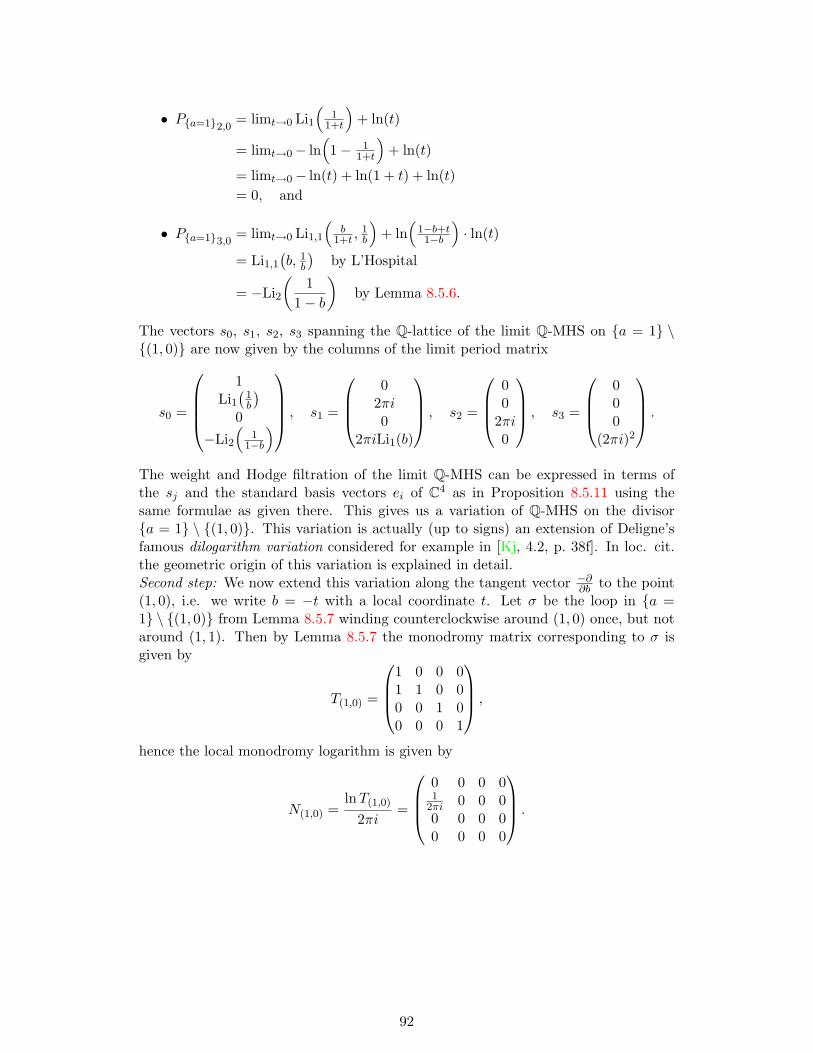
• Pa=12,0 = limt→0 Li1(

11+t

)+ ln(t)

= limt→0− ln(1− 1

1+t

)+ ln(t)

= limt→0− ln(t) + ln(1 + t) + ln(t)= 0, and

• Pa=13,0 = limt→0 Li1,1(

b1+t ,

1b

)+ ln

(1−b+t1−b

)· ln(t)

= Li1,1(b, 1b

)by L’Hospital

= −Li2

(1

1− b

)by Lemma 8.5.6.

The vectors s0, s1, s2, s3 spanning the Q-lattice of the limit Q-MHS on a = 1 \(1, 0) are now given by the columns of the limit period matrix

s0 =

1

Li1(

1b

)0

−Li2(

11−b

) , s1 =

0

2πi0

2πiLi1(b)

, s2 =

00

2πi0

, s3 =

000

(2πi)2

.

The weight and Hodge filtration of the limit Q-MHS can be expressed in terms ofthe sj and the standard basis vectors ei of C4 as in Proposition 8.5.11 using thesame formulae as given there. This gives us a variation of Q-MHS on the divisora = 1 \ (1, 0). This variation is actually (up to signs) an extension of Deligne’sfamous dilogarithm variation considered for example in [Kj, 4.2, p. 38f]. In loc. cit.the geometric origin of this variation is explained in detail.Second step: We now extend this variation along the tangent vector −∂∂b to the point(1, 0), i.e. we write b = −t with a local coordinate t. Let σ be the loop in a =1 \ (1, 0) from Lemma 8.5.7 winding counterclockwise around (1, 0) once, but notaround (1, 1). Then by Lemma 8.5.7 the monodromy matrix corresponding to σ isgiven by

T(1,0) =

1 0 0 01 1 0 00 0 1 00 0 0 1

,

hence the local monodromy logarithm is given by

N(1,0) =lnT(1,0)

2πi=

0 0 0 01

2πi 0 0 00 0 0 00 0 0 0

.

92

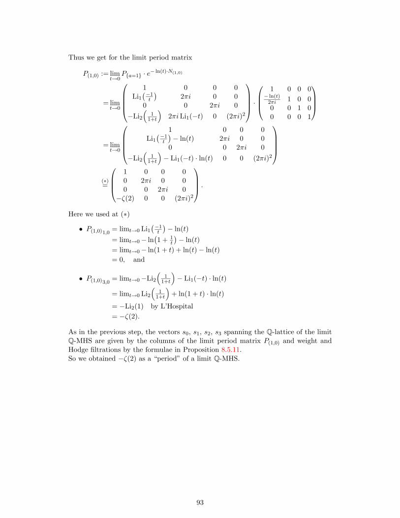
Thus we get for the limit period matrix

P(1,0) := limt→0

Pa=1 · e− ln(t)·N(1,0)

= limt→0

1 0 0 0

Li1(−1t

)2πi 0 0

0 0 2πi 0−Li2

(1

1+t

)2πiLi1(−t) 0 (2πi)2

·

1 0 0 0− ln(t)

2πi 1 0 00 0 1 00 0 0 1

= limt→0

1 0 0 0

Li1(−1t

)− ln(t) 2πi 0 0

0 0 2πi 0−Li2

(1

1+t

)− Li1(−t) · ln(t) 0 0 (2πi)2

(∗)=

1 0 0 00 2πi 0 00 0 2πi 0

−ζ(2) 0 0 (2πi)2

.

Here we used at (∗)

• P(1,0)1,0= limt→0 Li1

(−1t

)− ln(t)

= limt→0− ln(1 + 1

t

)− ln(t)

= limt→0− ln(1 + t) + ln(t)− ln(t)= 0, and

• P(1,0)3,0= limt→0−Li2

(1

1+t

)− Li1(−t) · ln(t)

= limt→0 Li2(

11+t

)+ ln(1 + t) · ln(t)

= −Li2(1) by L’Hospital= −ζ(2).

As in the previous step, the vectors s0, s1, s2, s3 spanning the Q-lattice of the limitQ-MHS are given by the columns of the limit period matrix P(1,0) and weight andHodge filtrations by the formulae in Proposition 8.5.11.So we obtained −ζ(2) as a “period” of a limit Q-MHS.

93

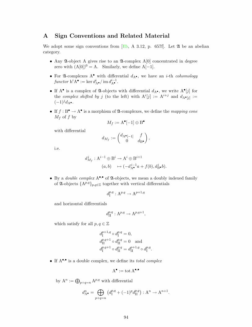
A Sign Conventions and Related Material

We adopt some sign conventions from [Eb, A 3.12, p. 657f]. Let A be an abeliancategory.

• Any A-object A gives rise to an A-complex A[0] concentrated in degreezero with (A[0])0 = A. Similarly, we define A[−1].

• For A-complexes A• with differential dA• , we have an i-th cohomologyfunctor hiA• := ker diA•/ im di−1

A• .

• If A• is a complex of A-objects with differential dA• , we write A•[j] forthe complex shifted by j (to the left) with Ai[j] := Ai+j and dA•[j] :=(−1)jdA• .

• If f : B• → A• is a morphism of A-complexes, we define the mapping coneMf of f by

Mf := A•[−1]⊕ B•

with differential

dMf:=(dA•[−1] f

0 dB•

),

i.e.

d iMf: Ai−1 ⊕ Bi → Ai ⊕ Bi+1

(a, b) 7→ (−d i−1A• a+ f(b), d iB•b).

• By a double complex A•,• of A-objects, we mean a doubly indexed familyof A-objects Ap,qp,q∈Z together with vertical differentials

dp,qI : Ap,q → Ap+1,q

and horizontal differentials

dp,qII : Ap,q → Ap,q+1,

which satisfy for all p, q ∈ Z

dp+1,qI dp,qI = 0,

dp,q+1II dp,qII = 0 and

dp,q+1I dp,qII = dp+1,q

II dp,qI .

• If A•,• is a double complex, we define its total complex

A• := tot A•,•

by An :=⊕

p+q=n Ap,q with differential

dnA• =⊕p+q=n

(dp,qI + (−1)pdp,qII

): An → An+1.

94

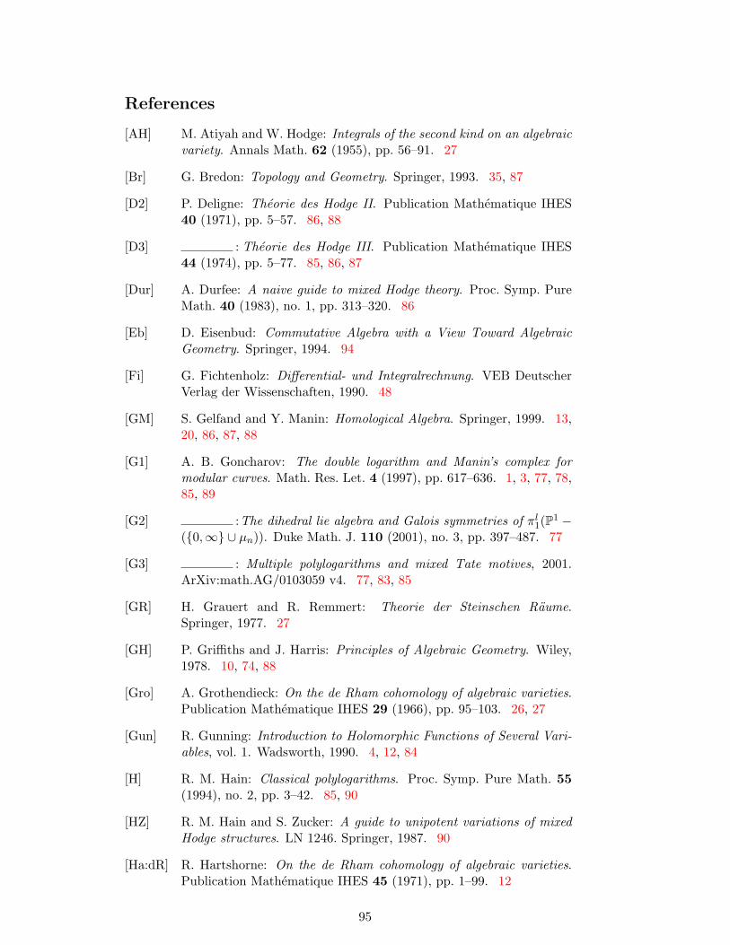
References

[AH] M. Atiyah and W. Hodge: Integrals of the second kind on an algebraicvariety. Annals Math. 62 (1955), pp. 56–91. 27

[Br] G. Bredon: Topology and Geometry. Springer, 1993. 35, 87

[D2] P. Deligne: Theorie des Hodge II. Publication Mathematique IHES40 (1971), pp. 5–57. 86, 88

[D3] : Theorie des Hodge III. Publication Mathematique IHES44 (1974), pp. 5–77. 85, 86, 87

[Dur] A. Durfee: A naive guide to mixed Hodge theory. Proc. Symp. PureMath. 40 (1983), no. 1, pp. 313–320. 86

[Eb] D. Eisenbud: Commutative Algebra with a View Toward AlgebraicGeometry. Springer, 1994. 94

[Fi] G. Fichtenholz: Differential- und Integralrechnung. VEB DeutscherVerlag der Wissenschaften, 1990. 48

[GM] S. Gelfand and Y. Manin: Homological Algebra. Springer, 1999. 13,20, 86, 87, 88

[G1] A. B. Goncharov: The double logarithm and Manin’s complex formodular curves. Math. Res. Let. 4 (1997), pp. 617–636. 1, 3, 77, 78,85, 89

[G2] :The dihedral lie algebra and Galois symmetries of πl1(P1 −(0,∞ ∪ µn)). Duke Math. J. 110 (2001), no. 3, pp. 397–487. 77

[G3] : Multiple polylogarithms and mixed Tate motives, 2001.ArXiv:math.AG/0103059 v4. 77, 83, 85

[GR] H. Grauert and R. Remmert: Theorie der Steinschen Raume.Springer, 1977. 27

[GH] P. Griffiths and J. Harris: Principles of Algebraic Geometry. Wiley,1978. 10, 74, 88

[Gro] A. Grothendieck: On the de Rham cohomology of algebraic varieties.Publication Mathematique IHES 29 (1966), pp. 95–103. 26, 27

[Gun] R. Gunning: Introduction to Holomorphic Functions of Several Vari-ables, vol. 1. Wadsworth, 1990. 4, 12, 84

[H] R. M. Hain: Classical polylogarithms. Proc. Symp. Pure Math. 55(1994), no. 2, pp. 3–42. 85, 90

[HZ] R. M. Hain and S. Zucker: A guide to unipotent variations of mixedHodge structures. LN 1246. Springer, 1987. 90

[Ha:dR] R. Hartshorne: On the de Rham cohomology of algebraic varieties.Publication Mathematique IHES 45 (1971), pp. 1–99. 12

95

[Ha] :Algebraic Geometry. Springer, 1977. 4, 5, 6, 7, 8, 12, 17,18, 19, 27, 31, 42, 54, 58, 61, 67, 70, 87, 89

[Hi1] H. Hironaka: Resolution of singularities. Annals Math. 79 (1964),pp. 109–326. 27, 59

[Hi2] : Triangulation of algebraic sets. In: Algebraic Geometry,Arcata 1974, vol. 29 of Proc. Symp. Pure Math., pp. 165–185. AMS,1975. 46, 49, 53, 54

[HW] A. Huber and J. Wildeshaus: The classical polylogarithm,abstract of a series of lectures given at the workshop onpolylogs in Essen, 1997. Available online at http://www.mathematik.uni-leipzig.de/~huber/preprints/essen.dvi.77

[Hui] J. Huisman: Real algebraic differential forms on complex algebraicvarieties. Indag. Math. (N.S.) 11 (2000), no. 1, pp. 63–71. 62

[Kj] T. Kleinjung: Gerahmte gemischte Tate-Motive und die Werte vonZetafunktionen zu Zahlkorpern an den Stellen 2 und 3. Ph.D. thesis,Rheinische Friedrich-Wilhelms-Universitat Bonn, Bonner Mathema-tische Schriften, Nr. 340, ISSN 0524-045X, 2000. 78, 86, 92

[K] M. Kontsevich: Operads and motives in deformation quantisation.Letters in Mathematical Physics 48 (1999), pp. 35–72. 1, 2, 43, 45,46, 48, 62, 63, 65, 66, 67, 68

[KZ] M. Kontsevich and D. Zagier: Periods. In: B. Engquis andW. Schmid, editors, Mathematics unlimited – 2001 and beyond, pp.771–808. Springer, 2001. 43, 47, 48

[KB] B. Koopman and A. Brown: On the covering of analytic loci by com-plexes. Trans. Amer. Math. Soc. 34 (1932), pp. 231–251. 54

[Ma] H. Matsumura: Commutative Algebra. W.A. Benjamin, 1970. 12

[Sb] A. Seidenberg: A new decision method for elementary algebra. AnnalsMath. 60 (1954), no. 2, pp. 365–374. 49, 54

[Se:gaga] J.-P. Serre: Geometrie algebrique et geometrie analytic. Ann. Inst.Four. 6 (1956), pp. 1–42. 6

[Se] :A Course in Arithmetic. Springer, 1973. 70, 72

[Sil] J. Silverman: The Arithmetic of Elliptic Curves. Springer, 1986. 72,73, 74

[St] J. Steenbrink: A summary of mixed Hodge theory. Proc. Symp. PureMath. 55 (1994), no. 1, pp. 31–41. 90

[W] F. Warner: Foundations of Differentiable Manifolds and Lie Groups.Springer, 1983. 10

96

[Z1] J. Zhao: Multiple polylogarithms: analytic continuation, monodromy,and variations of mixed Hodge structures. In: Contemporary trendsin algebraic geometry and algebraic topology (Tianjin, 2000), vol. 5of Nankai Tracts Math., pp. 167–193. World Sci. Publishing, RiverEdge, NJ, 2002. 77, 78, 90

[Z2a] : Analytic continuation of multiple polylogarithms, 2003.ArXiv:math.AG/0302054 v2. 78, 83, 85, 89

[Z2b] :Variations of Mixed Hodgestructures of Multiple Polyloga-rithms, 2003. ArXiv:math.AG/0302055 v3. 78, 85, 90, 91

Glossary of Notations

|X| set of closed points of a variety X, 4

M sheaf associated to a module M , 5

〈 · , · 〉 homology-cohomology-pairing, 41

A[0] complex concentrated in degree zero with (A[0])0 = A, 94

A•[j] complex shifted by j, 94

an functor yielding the associated complex analytic space, 4

Ank affine n-space over a field k, 42

CPn complex projective space in the category of schemes, 5

CPnan complex projective space in the category of complex analyticspaces, 5

CX constant sheaf with fibre C on a space X, 10

Cpsing(M ; C) C-vector space of singular p-cochains of a space M , 11

Cpsing(M ; C) sheaf of singular p-cochains of a space M , 11

Cp(U, ?) Cech functor, 18

Cp(U;F) Cech group of a sheaf F , 18

Cpsing(Xan, Dan; C) sheaf of singular p-cochains of a pair (Xan, Dan), 32

C∞p (M ; C) C-vector space of smooth singular p-chains of a complexmanifold M , 34

Csingp (M ; C) C-vector space of singular p-chains of a space M , 34

Cp∞(M ; C) C-vector space of smooth singular p-cochains of a complex

manifold M , 34

Cp∞(M ; C) sheaf of smooth singular p-cochains of a complex manifoldM , 34

97

C•,•∞ (Dan; C) double complex of sheaves of smooth singular cochains ofDan•, 35

C•∞(Dan; C) complex of sheaves of smooth singular cochains of a divisorDan, 35

C•∞(Xan, Dan; C) complex of sheaves of smooth singular cochains of a pair(Xan, Dan), 35

Di0 ... ip intersection of Di0 , · · · , Dip , 12

DI intersection of Di for i ∈ I, 12

D• simplicial scheme associated to a divisor D, 13

D closed covering (Dani )ri=1, 30

4 interior of a simplex or a point, 53

4stdp standard p-simplex, 53

∆ triple coproduct, 66

E•M classical deRham complex of a complex manifold M , 10

ev evaluation morphism P+ → C, 64

G•F Godement resolution of a sheaf F , 8

G•F• Godement resolution of a complex of sheaves F•, 8

Γp top-dimensional part of a p-chain Γ ∈ C∞p (Xan, Dan; Q), 44

H•dR(M ; C) analytic deRham cohomology of a complex manifold M , 11

H•(M ; C) complex cohomology of a space M , 11

H•dR(X/k) algebraic deRham cohomology of a smooth variety X, 12

H•dR(D/k) algebraic deRham cohomology of a divisor D, 14

H•dR(X,D/k) algebraic deRham cohomology of a pair (X,D), 15

Hp(U;F) Cech cohomology of a sheaf F , 18

Hp(F•) sheafified hypercohomology of a complex of sheaves F•, 20

H•dR(Dan; C) analytic deRham cohomology of a divisor Dan, 24

H•dR(Xan, Dan; C) analytic deRham cohomology of a pair (Xan, Dan), 24

H•(Xan, Dan; C) complex cohomology of a pair (Xan, Dan), 28

H•sing(M ; C) singular cohomology of a space M , 32

H•sing(Xan, Dan; C) singular cohomology of a pair (Xan, Dan), 32

H•∞(M ; C) smooth singular cohomology of a complex manifold M , 34

98

H•∞(Dan; C) smooth singular cohomology of a divisor Dan, 35

H•∞(Xan, Dan; C) smooth singular cohomology of a pair (Xan, Dan), 35

H∞• (M ; C) smooth singular homology of a complex manifold M , 40

H∞• (Dan; C) smooth singular homology of a divisor Dan, 40

H∞• (Xan, Dan; C) smooth singular homology of a pair (Xan, Dan), 40

hiA• i-th cohomology of a complex A•, 94

MC mapping cone of CXan → i∗CDan , 28

M•sing mapping cone of C•sing(Xan; C) −→ i∗C•sing(D

an; C), 38

Ω•M analytic deRham complex of a complex manifold M , 10

Ω•X/k algebraic deRham complex of a variety X, 12

Ω•,•D•/k algebraic double deRham complex of D•, 14

Ω•D/k algebraic deRham complex of a divisor D, 14

Ω•X,D/k algebraic deRham complex of a pair (X,D), 15

Ω•,•Dan• analytic double deRham complex of Dan•, 24

Ω•Dan analytic deRham complex of a divisor Dan, 24

Ω•Xan,Dan analytic deRham complex of a pair (Xan, Dan), 24

Pp set of all pairing periods, 43

P ′p set of all special pairing periods, 43

Pa set of all abstract periods, 45

Pn set of all naıve periods, 46

P equal to Pa, P ′p and Pn, 62

P+ Q-vector space of effective periods, 63

P P+ adjoint 12πi , 66

Q integral closure of Q in R, 46

Q-MHS abbreviation for mixed Q-Hodge structure, 85

Simplex category with objects [m] and <-preserving maps, 13

totA•,• total complex of a double complex A•,•, 94

U open covering (Uj)j∈J , 18

Ui0 ... im intersection of Ui0 , . . . , Uim , 18

UI intersection of Ui for i ∈ I, 18

U• simplicial scheme associated to an open covering U, 19

99

Index

a-period, see Period, abstract

Cechcohomology, 18functor, 18group, 18

Coherent sheaf, 5Complex analytic space, 4

associated, 4Complex cohomology, 11, 28

DeRham cohomologyalgebraic, 12, 14, 15analytic, 11, 24classical, 10

DeRham complexalgebraic, 12analytic, 10classical, 10

Dilogarithm, 77Divisor

with normal crossings, 12Double complex, 94

Elliptic curves, 72

Godement resolution, 8

Hyperlogarithm, 77

Logarithmdouble, 77

Mapping cone, 94Mixed Q-Hodge structure, 85

n-period, see Period, naıve

p-period, see Period, pairingp′-period, see Period, pairing, specialPeriod

abstract, 45effective, 63matrix, 43naıve, 46pairing, 43

special, 43Polylogarithm

multiple, 77

Q-MHS, see Mixed Q-Hodge structureQuadratic form, 70

discriminant of, 72

Semi-algebraicmap, 49set, 46

Simplexopen, 53smooth, 34

Simplicial scheme, 13Singular cohomology, 11, 32Smooth singular cohomology, 34Smooth singular homology, 40

Torsor, 62Total complex, 94Triple coproduct, 66, 68

Variation of mixed Q-Hodge structures,90

Variety, 3

ζ-value, 48, 75

100

Erklarung

Ich versichere, dass ich die vorliegende Arbeit selbststandig und nur unter Verwendungder angegebenen Quellen und Hilfsmittel angefertigt habe.Diese Arbeit wurde in dieser oder ahnlicher Form noch keiner anderen Prufungsbe-horde vorgelegt.

Ort Datum Unterschrift

101