permutation spreading technique employing spatial ... · permutation spreading technique employing...
TRANSCRIPT

Permutation Spreading Technique
Employing Spatial Modulation
For MIMO-CDMA Systems
by
Nordine Quadar
Thesis submitted in partial fulfillment of the requirements
For the Master of Applied Science degree in
Electrical and Computer Engineering
School of Electrical Engineering and Computer Science
Faculty of Engineering
University of Ottawa
c© Nordine Quadar, Ottawa, Canada, 2017

In the name of Allah, the Most Gracious and the Most Merciful
ii
Abstract
Spatial Modulation (SM) is a spatial multiplexing technique designed for MIMO sys-
tems where only one transmit antenna is used at each time. It is considered to be an
attractive choice for future wireless communication systems as it reduces Inter-Channel
Interference (ICI) while maintaining high energy efficiency. It can achieve this goal by
mapping block of data bits into constellation points in the spatial and signal domain.
Combining this innovative method with multiple access techniques could improve the sys-
tem performance and enhance the data rate. In Code Division Multiple Access (CDMA)
method employing parity bit permutation spreading, the bit error rate (BER) performance
could be improved by using the parity bits to select the spreading sequence to use at each
signaling interval. In this thesis, a new system model based on SM and CDMA employing
parity bit permutation spreading is proposed and investigated. The proposed system takes
advantage of the benefits of both techniques.
In this system, in addition to use the parity bits to select the spreading sequences, same
concept is used to select the combination of antennas to activate at each time instant. By
doing so, a reduction of power consumption, Inter-Channel and Inter Symbol Interference
effect can be achieved while keeping a certain diversity order compared to SM. Multiuser
scenario is also discussed in order to investigate the multiple access interference (MAI)
effects in synchronous transmission. In such case, the receiver estimates the desired user’s
information by considering the other users’ signal as additional noise.
Simulation results of the proposed MIMO-CDMA system employing permutation spread-
ing show, for single user and multiuser, a significant improvement of the BER performance
in low signal to noise ratio (SNR) when SM is implemented.
iii

Acknowledgements
First and foremost, I would like to thank Allah Almighty for his blessing and giving me
the power to accomplish this milestone.
I would like to express my deepest gratitude and sincere appreciation to my supervisor
Dr. Claude D’Amours for his support, guidance, valuable advices and encouragement
throughout this research. Without his help, this thesis would not have been achievable. I
feel very privileged having such a mentor.
Last but not least, I would like to thank my beloved wife Manal for her love, patience
and continued support. Special thanks go to my mother for her prayers, blessings and
unconditional love. I am also grateful to all my family members for their support.
iv

To the loving memory of my father,
To my soon-to-be-born baby.
v
Table of Contents
List of Tables ix
List of Figures x
List of Abbreviations xiii
List of Symbols xvi
1 Introduction 1
1.1 Motivation and background . . . . . . . . . . . . . . . . . . . . . . . . . . 1
1.2 Thesis scope . . . . . . . . . . . . . . . . . . . . . . . . . . . . . . . . . . . 4
1.3 Thesis objectives . . . . . . . . . . . . . . . . . . . . . . . . . . . . . . . . 5
1.4 Scientific methods employed . . . . . . . . . . . . . . . . . . . . . . . . . . 6
1.5 Thesis contributions . . . . . . . . . . . . . . . . . . . . . . . . . . . . . . 6
1.6 Thesis organisation . . . . . . . . . . . . . . . . . . . . . . . . . . . . . . . 7
2 Permutation Spreading For MIMO-CDMA System 9
2.1 Introduction . . . . . . . . . . . . . . . . . . . . . . . . . . . . . . . . . . 9
2.2 System Model . . . . . . . . . . . . . . . . . . . . . . . . . . . . . . . . . . 10
2.2.1 Transmitter Model . . . . . . . . . . . . . . . . . . . . . . . . . . . 10
vi
2.2.2 Receiver Model . . . . . . . . . . . . . . . . . . . . . . . . . . . . . 14
2.3 Theoretical analysis of the BER performance . . . . . . . . . . . . . . . . . 19
2.3.1 BER analysis for MIMO-CDMA system with parity bit selected
spreading . . . . . . . . . . . . . . . . . . . . . . . . . . . . . . . . 19
2.3.2 BER analysis for MIMO-CDMA system with Permutation Spreading 20
2.4 Simulation results and discussion . . . . . . . . . . . . . . . . . . . . . . . 21
2.4.1 Discussion . . . . . . . . . . . . . . . . . . . . . . . . . . . . . . . . 25
3 Spatial Modulation 26
3.1 Introduction . . . . . . . . . . . . . . . . . . . . . . . . . . . . . . . . . . 26
3.2 Spatial Modulation (SM) system model . . . . . . . . . . . . . . . . . . . . 28
3.2.1 Transmitter Model . . . . . . . . . . . . . . . . . . . . . . . . . . . 28
3.2.2 Receiver model . . . . . . . . . . . . . . . . . . . . . . . . . . . . . 31
3.3 Generalized Spatial Modulation (GSM) system model . . . . . . . . . . . . 33
3.3.1 Transmitter Model . . . . . . . . . . . . . . . . . . . . . . . . . . . 33
3.3.2 Receiver Model . . . . . . . . . . . . . . . . . . . . . . . . . . . . . 35
3.4 Receiver complexity . . . . . . . . . . . . . . . . . . . . . . . . . . . . . . . 36
3.5 Simulation results and discussion . . . . . . . . . . . . . . . . . . . . . . . 37
3.5.1 Discussion . . . . . . . . . . . . . . . . . . . . . . . . . . . . . . . . 41
4 Single User Permutation Spreading Employing Spatial Modulation for
MIMO-CDMA system 42
4.1 Introduction . . . . . . . . . . . . . . . . . . . . . . . . . . . . . . . . . . 42
4.2 System Model . . . . . . . . . . . . . . . . . . . . . . . . . . . . . . . . . . 43
4.2.1 Transmitter Model . . . . . . . . . . . . . . . . . . . . . . . . . . . 43
4.2.2 Receiver Model . . . . . . . . . . . . . . . . . . . . . . . . . . . . . 47
vii

4.3 Theoretical analysis of the BER performance . . . . . . . . . . . . . . . . . 52
4.3.1 MISO-CDMA system . . . . . . . . . . . . . . . . . . . . . . . . . . 52
4.3.2 MIMO-CDMA system . . . . . . . . . . . . . . . . . . . . . . . . . 56
4.4 Simulation results and discussion . . . . . . . . . . . . . . . . . . . . . . . 57
4.4.1 Theoretical and Simulation results of MIMO/CDMA with SM design 57
4.4.2 Comparison of simulation results . . . . . . . . . . . . . . . . . . . 58
4.4.3 Discussion . . . . . . . . . . . . . . . . . . . . . . . . . . . . . . . . 63
5 Multiuser Permutation Spreading Employing Spatial Modulation For
Synchronous MIMO-CDMA systems 64
5.1 Introduction . . . . . . . . . . . . . . . . . . . . . . . . . . . . . . . . . . 64
5.2 System Model . . . . . . . . . . . . . . . . . . . . . . . . . . . . . . . . . . 65
5.2.1 Transmitter Model . . . . . . . . . . . . . . . . . . . . . . . . . . . 65
5.2.2 Receiver Model . . . . . . . . . . . . . . . . . . . . . . . . . . . . . 66
5.3 Simulation results and discussion . . . . . . . . . . . . . . . . . . . . . . . 69
5.3.1 Simulation results comparison . . . . . . . . . . . . . . . . . . . . . 69
5.3.2 Discussion . . . . . . . . . . . . . . . . . . . . . . . . . . . . . . . . 71
6 Conclusion and suggestion for future work 73
6.1 Conclusion . . . . . . . . . . . . . . . . . . . . . . . . . . . . . . . . . . . . 73
6.2 Potential future work . . . . . . . . . . . . . . . . . . . . . . . . . . . . . 74
References 76
viii

List of Tables
2.1 T-Design Permutations Spreading for MIMO-CDMA system with 4 transmit
antennas . . . . . . . . . . . . . . . . . . . . . . . . . . . . . . . . . . . . 12
2.2 STBC-Design Permutations Spreading for MIMO-CDMA system with 4
transmit antennas . . . . . . . . . . . . . . . . . . . . . . . . . . . . . . . . 13
2.3 STBC-Design Permutations Spreading transmit table for 4 transmit antennas 15
3.1 SM mapping table using BPSK and Nt=4 . . . . . . . . . . . . . . . . . . 30
3.2 SM mapping table using QPSK and Nt=4 . . . . . . . . . . . . . . . . . . 31
3.3 GSM mapping table using BPSK , Nt=5 and Na=2 . . . . . . . . . . . . . 35
3.4 VGSM mapping table using Nt=4 . . . . . . . . . . . . . . . . . . . . . . . 36
4.1 Permutation Spreading for MIMO-CDMA system with 4 transmit antennas
Using STBC design . . . . . . . . . . . . . . . . . . . . . . . . . . . . . . . 45
4.2 SM mapping table for MIMO system with four transmit antennas . . . . . 46
4.3 Permutation Spreading transmit table for 4x4 MIMO-CDMA system using
SM . . . . . . . . . . . . . . . . . . . . . . . . . . . . . . . . . . . . . . . . 48
4.4 Received vector for MISO system with four transmit antennas and one re-
ceiver antenna . . . . . . . . . . . . . . . . . . . . . . . . . . . . . . . . . . 53
ix
List of Figures
2.1 Transmitter of MIMO-CDMA with parity bit selected and permutation
spreading . . . . . . . . . . . . . . . . . . . . . . . . . . . . . . . . . . . . 11
2.2 Receiver of MIMO-CDMA with parity bit selected and permutation spreading 16
2.3 BER performance of MISO-CDMA System with parity bit selected spreading 22
2.4 BER performance of MIMO-CDMA System with parity bit selected spreading 22
2.5 BER performance of MISO-CDMA System with STBC permutation spreading 23
2.6 BER performance of MIMO-CDMA System with STBC permutation spread-
ing . . . . . . . . . . . . . . . . . . . . . . . . . . . . . . . . . . . . . . . . 23
2.7 BER performance comparison of MISO-CDMA System using the three tech-
niques . . . . . . . . . . . . . . . . . . . . . . . . . . . . . . . . . . . . . . 24
2.8 BER performance comparison of MIMO-CDMA System using the three
techniques . . . . . . . . . . . . . . . . . . . . . . . . . . . . . . . . . . . . 24
3.1 SM constellation diagram . . . . . . . . . . . . . . . . . . . . . . . . . . . 27
3.2 Working concepts of (a) SMX, (b) OSTBC, (c) SM and (d) GSSK . . . . . 29
3.3 Spatial Modulation system model . . . . . . . . . . . . . . . . . . . . . . . 30
3.4 Generalized Spatial Modulation system model . . . . . . . . . . . . . . . . 34
3.5 Comparison of receiver complexity between SM and GSM using ML detection 37
3.6 Comparison of SM performances, where Nt = 128 for η = 8bits, Nt = 32 for
η = 6bits, Nt = 8 for η = 4bits, using BPSK modulation and Nr = 4 . . . . 39
x
3.7 BER performance of SM, GSM and VGSM where η = 4bits, Nr = 4 and
using BPSK modulation. . . . . . . . . . . . . . . . . . . . . . . . . . . . . 39
3.8 BER performance of SM, GSM and VGSM where η = 6bits, Nr = 4 and
using BPSK modulation. . . . . . . . . . . . . . . . . . . . . . . . . . . . . 40
3.9 BER performance of SM, GSM and VGSM where η = 8bits, Nr = 4 and
using BPSK modulation. . . . . . . . . . . . . . . . . . . . . . . . . . . . . 40
4.1 The Transmitter of MIMO-CDMA with permutation spreading using SM . 44
4.2 Transmitter for a 4x4 MIMO-CDMA with permutation spreading using SM 46
4.3 Receiver of MIMO/CDMA with permutation spreading using SM . . . . . 49
4.4 Theoretical BER performance of 4x1 MISO-CDMA System using Permuta-
tion Spreading with conventional STBC design vs SM design . . . . . . . . 59
4.5 Theoretical BER performance of 4x4 MIMO-CDMA System using Permu-
tation Spreading with conventional STBC design vs SM design . . . . . . . 59
4.6 BER performance of MIMO-CDMA System with Permutation Spreading
using SM design . . . . . . . . . . . . . . . . . . . . . . . . . . . . . . . . . 60
4.7 BER performance of 4x1 MISO-CDMA System using Permutation Spread-
ing with conventional STBC design vs SM design . . . . . . . . . . . . . . 61
4.8 BER performance of 2x2 MIMO-CDMA System using Permutation Spread-
ing with conventional STBC design vs SM design . . . . . . . . . . . . . . 61
4.9 BER performance of 4x4 MIMO-CDMA System using Permutation Spread-
ing with conventional STBC design vs SM design . . . . . . . . . . . . . . 62
4.10 BER performance of MIMO-CDMA System using Permutation Spreading
with SM design vs Conventional SM techniques . . . . . . . . . . . . . . . 62
5.1 Multiuser transmitter of MIMO-CDMA with permutation spreading using
SM . . . . . . . . . . . . . . . . . . . . . . . . . . . . . . . . . . . . . . . . 67
5.2 Multiuser receiver of MIMO/CDMA with permutation spreading using SM 68
xi

5.3 Comparison of BER Performance of 4x4 MISO-CDMA System using SM
Permutation Spreading design . . . . . . . . . . . . . . . . . . . . . . . . . 71
5.4 Comparison of BER performance of 4x4 MISO-CDMA System using SM
Permutation Spreading design vs STBC design . . . . . . . . . . . . . . . . 72
xii

List of Abbreviations
AWGN Additive White Gaussian Noise
3GPP Third Generation Partnership Project
BER Bit Error Rate
BLAST Bell Labs Layered Space Time
BPSK Binary Phase Shift Keying
BS Base Station
CDMA Code Division Multi Access
CSI Channel State Information
DS-CDMA Direct Sequence Code Division Multiple Access
DS-SS Direct-Spread Spread Spectrum
FBE-SM Fractional Bit Encoded Spatial Modulation
GPRS General Packet Radio Service
Gbps Gigabit per second
GSM Generalized Spatial Modulation
GSSK General Space Shift Keying
ICI Inter-Channel Interference
IOT Internet Of Things
ISI Inter-symbol Interference
LDS Low Density Spreading
LPMA Lattice Partition Multiple Access
xiii
LLR Log Likelihood Ratio
LTE-A Long-Term Evolution Advanced
MAI Multi-Access Interference
MIMO Multiple-Input Multiple-Output
MISO Multiple-Input Single-Output
ML Maximum Likelihood
MRC Maximal Ratio Combiner
MLD Maximum Likelihood Detection
MUD Multiuser Detection
MUST Multiuser Superposition Transmission
NOMA Non-Orthogonal Multiple Access
OFDM Orthogonal Frequency Division Multiplexing
OMA Orthogonal Multiple Access
OSTBC Orthogonal Space Time Block Coding
pdf Probability Density Function
PDMA Pattern Division Multiple Access
PN Pseudo-Noise
QAM Quadrature Amplitude Modulation
QoS Quality Of Service
QPSK Quadrature Phase Shift Keying
RF Radio-Frequency
SCMA Sparse Code Multiple Access
SD Sphere Decoding
SM Spatial Modulation
SMX Spatial Multiplexing
SNR Signal To Noise Ratio
SS Spread Spectrum
SSK Space Shift Keying
STBC Space Time Block Code
TDMA Time Domain Multiple Access
xiv
UMTS Universal Mobile Telecommunication Service
VGSM Variable Generalized Spatial Modulation
VLS Visible Light Communication
WCDMA Wideband CDMA
xv

List of Symbols
Nt Number of transmit antennas
Nr Number of received antennas
Ncu Number of channels
Nm Number of transmitted symbols
s Transmitted symbol
Y Received matrix
n Complex Additive White Noise (AWGN)
H Channel gain vector
S Transmitted signal matrix
. Estimated symbol
p Antenna index
‖.‖ Absolute-value norm
yi Received vector at the ith received antenna
σ2n Noise variance
Na Number of antenna to activate(..
)The binomial operation
b.c Floor operation
ρ Number of antenna combinations
η Spectral efficiency
C Computational Complexity
R complexity ratio
xvi
wi Spreading waveform used by the ith transmit antenna
ci ith spreading waveform
Mi ith coset
L Number of messages per coset
K Number of cosets
mj Bit stream transmitted from the jth antenna
Eb Received energy per bit
αji Complex channel gain between the ith transmit antenna and the jth received antenna
b(k)i The ith message bits from the kth message vector
rkl Output of the lth matched filter at the receive antenna
U Decision variable
rx Received signal
E0 Noise spectral density
M Number of cosets
d Euclidean distance
γ Average received SNR per bit
dq[i] Data bit streams
Q Number of users q
wqi Spreading sequences used by the ith transmit antenna of user q
T Bit duration
pqn Pseudo-noise generated code of the qth user
x Average received energy per bit
xvii
Chapter 1
Introduction
1.1 Motivation and background
These days, wireless communications is prevalent everywhere in the world and much of our
business and entertainment activities are dependent on wireless communication services.
The demand for these services continues to grow at a rapid pace and service providers are
expected to be able to accommodate a large increase in the number of users with increased
data rate requirements. With the development of the Internet of things (IoT), Ericsson
has announced that more than 50 billion devices will be connected to the network by 2020
[1]. Therefore, future wireless network should be able to face the tremendous increase of
the traffic.
Looking past, wireless communication technologies have witnessed four generations of
technology evolution. The first generation system (1G) was introduced in 1980s and was
designed to support voice transmission using analog cellular technology. 1G was replaced
by the second generation (2G) because it had many limitations such as a poor voice qual-
ity, low transmission speed and no encryption. The 2G systems, also known as the Global
System for Mobile communications (GSM), started to expand all over the world in 1991.
Contrary to 1G, the second generation is designed based on digital cellular technologies,
which helped to enhance the spectral efficiency of the communication system. Text mes-
saging service was first introduced in GSM and a later release allowed low speed data
1

transmission using General Packet Radio Service (GPRS). The increasing number of 2G
users caused an increasing demand for high-speed data access. To face this issue, the third
generation (3G) came to life in 2001 with a service that can support data rate up to 2Mbps
[2]. The evolution of 3G for CDMA (Code Division Multiple Access) led to CDMA2000,
which is an improved version of CDMA used in 2G. The second widely used 3G technology
is the WCDMA (Wideband CDMA), also called UMTS (Universal Mobile Telecommuni-
cation Service). Although the 3G systems provide high-speed data service, the increasing
number of connected devices and the diversity of content to transmit have required higher
transmission speed and date rate. Therefore, new generation technology was needed in
order to align with the increasing demand. Forth generation (4G), also called long-term
evolution advanced (LTE-A), was launched in 2011 with a main goal to increase the trans-
mission speed by 10-bold compare to 3G and use channel bandwidth up to 20Mhz [3]. 4G
was able to achieve this goal by using multiple-input multiple-output (MIMO) technology
and advanced orthogonal multiple access (OMA) techniques such as orthogonal frequency
division multiplexing (OFDM). Moreover, 4G can achieve a data rate up to 1Gbps for low
mobility applications and up to 100Mbps for high mobility applications [3] [4]. As men-
tioned before, in the coming years the traffic of wireless communication will be enormously
increasing and the boundary of the 4G is approaching. Therefore, a lot of active researches
are shifting the focus towards the fifth generation (5G).
The 5G systems are expected to solve problems such as poor quality of service (QoS),
bad interconnectivity and poor coverage [5]. Although the 5G still a concept, its standard-
isation is expected to be ready by 2020. Compared to 4G, 5G systems will be designed in
order to achieve a system capacity 1000 times higher and to increase the average through-
put, spectral efficiency, data rate and the power efficiency by 10-bold [5]. Moreover, 5G
systems should insure a system latency that is below 1ms and be able to provide a data
bit rate up to 10Gbps [6]. A lot of research papers have been started to investigate the
possibility of adapting the existing technologies or suggesting new ones. For example in [6],
the author discusses some promising technologies for cellular architecture that can be em-
ployed for 5G systems such as femtocells, macrocells, relays and small sells. Furthermore,
several recent papers have discussed some new technologies that can be deployed in 5G
2
systems in order to achieve the expected requirements such as visible light communication
(VLS), mm-wave communication, massive MIMO technology and spatial modulation (SM)
technology [6] [7] [8].
According to many researches, MIMO systems are able to achieve high data rate without
any increase in the transmit power or the utilization [8], [9]. However, MIMO systems
will require more power amplifiers, RF chains, filters etc., which will decrease the power
efficiency of the system. That is why designing a MIMO system that have a fair tradeoff
between the spectral efficiency and the power efficiency is greatly needed. SM technique has
proven to be one of potential technologies that can achiever this challenging task. Its basic
idea is to activate one transmit antennas at each signaling interval and use the antenna
index as additional modulation scheme [10]. Taking the advantage of the single-RF chain
design and using the transmit antenna array, SM has shown in some recent studies that it
can outperform many conventional MIMO systems with less active transmit antennas [11],
[12].
Another key factor that could enable future networks to achieve the best spectrum
utilization is designing innovative modulation schemes. Traditionally, Orthogonal Multi-
ple Access (OMA) techniques have been used to increase the number of users that can
share the same spectrum. These OMA techniques use the orthogonal characteristic to
avoid the Multiple-Access Interference (MAI), which can be reached in different domains
such as frequency, time, space and code domains. Motivated by this concept, three tech-
niques such as Direct Sequence Code Division Multiple Access (DS-CDMA), Orthogonal
Frequency Domain Division (OFDM) and Time Domain Multiple Access (TDMA) have
been developed and used in many standards. Based on these techniques, recent researches
have proposed modified version of OMA that can be employed in future networks. These
techniques include Sparse Code Multiple Access (SCMA) [13], Low Density Spreading
(LDS) [14], Pattern Division Multiple Access (PDMA) [15] and Lattice Partition Multiple
Access (LPMA) [16]. A recent Multiple-access technique, called Non-Orthogonal Multiple
Access (NOMA), shows potential performance compared to the conventional OMA [17].
Unlike OMA where the orthogonality is the key to separate users of the same spectrum,
3

NOMA encourages using non-orthogonal separation. For instance, in CDMA it is required
to use different spreading codes that are orthogonal, whereas in NOMA users are allowed
to use the same spreading codes. This new technique has been proposed in the 3rd genera-
tion partnership project (3GPP) LTE standard under the name of Multiuser Superposition
Transmission (MUST) [18]. Exploiting all these concepts can lead to achieve the goal and
design new methods that can enhance the system performance.
1.2 Thesis scope
As discussed in [23], some of the main goals of the future wireless communication gen-
erations are to increase data rates and decrease system latency while keeping low power
consumption. Thus, modern modulation techniques must be able to comply with these re-
quirements. As previously discussed, SM-MIMO systems can achieve the fixed goal based
on two concepts:
• Reducing the number of transmit antennas in order to decrease the power consump-
tion by using less RF chains.
• Increasing data rates by providing additional modulation scheme.
CDMA systems were designed based on Direct-Spread Spread Spectrum (DS-SS) where
each user is assigned with a unique spreading waveform called chip. This signature is
used to spread the user’s transmit signal over a bandwidth that is larger than its original
bandwidth. At the receiver, the unique signature is used to separates users’ signals. If
the used spreading sequences are not orthogonal, the system will suffer from the MAI
effect, which will decrease the system performance. Inspired by this concept, a modified
version that uses parity bits to select the spreading waveforms is introduced in [22]. This
methods shows that a coding gain can be achieved by combining coding with spreading
code selection.
Combining the SM with Multiple-access techniques could improve their performance.
Several works, e.g., [19], [20], studied the possibility of employing SM design with OFDM
4

and SC-FDMA, but few papers has investigate the performance of SM when CDMA is
used [21]. Therefore, this study focuses on designing a new SM based on parity bit CDMA
technique.
1.3 Thesis objectives
This thesis aims to investigate the possibility of combining the SM-MIMO technique with
the CDMA version introduced in [22]. As discussed in the previous sections, power and
spectral efficiency are the key success of the future communication networks. SM uses the
single-RF chain design to decrease the number of active transmit antennas and therefore
increase the power efficiency. Moreover, it increases the data rate by using the transmit
antenna array as an additional modulation scheme. In the other hand, the CDMA parity
bit selection method adds a significant coding gain to the system and increases the spectral
efficiency. Motivated by these two techniques, this thesis proposes an adapted version of
SM-MIMO for CDMA parity bit selection system. Although, these two methods belong
to two different families; however, they share the same concept of using an index variable
as an additional parameter to convey the data bits. The proposed method should provide
all benefits of SM-MIMO and the CDMA parity bit selection methods.
The objective of this study is to propose a modified version of the SM-MIMO technique
that can be implemented using CDMA. Moreover, the thesis evaluates the bit error rate
(BER) performance of the new technique under frequency-nonselective Rayleigh fading
channels. The proposed system should be able to increase the BER performance compared
to the conventional STBC parity bit permutation spreading design. Also, it should increase
the power efficiency by proposing an optimal number of transmit antennas to activate in
order to ensure a certain diversity order while reducing the number of RF-chains. Addi-
tionally, this thesis should study the MAI effect in synchronous transmission for multiuser
scenarios and verify that the new design outperform the parity bit selection method of the
MIMO-CDMA discussed in [22] when SM is implemented. Inspired from NOMA technique,
the proposed system suggest that all users use the same spreading codes to transmit their
5

data bit where quasi-orthogonal codes are used to separate the users’ signals. By doing so,
there will be no need to increase the length of chips used when more users are added to
the same spectrum.
1.4 Scientific methods employed
The main purpose of this work is to provide a new design of the SM-MIMO system that
can be implemented with the parity bit selection CDMA method. A mathematical model
has been derived for the proposed system in order to evaluate the BER performance. The
proposed system model has been tested via computer simulations under fading channels
to confirm the mathematical derived model. The simulation results are compared with the
theoretical results and the conventional methods in order to evaluate the overall improve-
ment of the new method. Moreover, the system has been tested in multiuser scenarios and
compared with the parity bit selection CDMA technique.
1.5 Thesis contributions
The key contributions of this thesis is the design of a SM-MIMO system based on the
CDMA permutation spreading technique. The proposed system provides the benefits of
the SM method and the permutation spreading method. It helps to increases the system
performance in terms of spectral and power efficiency by reducing the number of transmit
antenna to activate and using the permutation spreading method to provide additional
coding gain.
The following are the key contributions of this thesis:
• Proposal of a modified version of the MIMO-CDMA spreading permutation technique
when SM method is used.
• Proposal of new design strategy for the transmit antenna selection in SM-MIMO
system. The design strategy is based on Space Time Block Code (STBC) permutation
6
discussed in [24].
• The theoretical analysis of the BER performance of the proposed system in a single
user scenario and over frequency non-selective fading channels.
• Simulations comparison and performance evaluation of the new method and the
conventional methods.
• Investigation of MAI effect on the BER performance for synchronous transmission. In
this scenario, all users are assumed to use the same spreading sequences and signature
codes, also called pseudo-noise (PN), are used to separate the users’ signals.
1.6 Thesis organisation
The remainder of this thesis is organised as follows:
• Chapter 2 introduces the basic idea of two parity bit selection methods for MIMO-
CDMA systems: parity bit selected spreading and permutation spreading techniques.
In this chapter, different design strategies such as STBC design and T-design are
explained. Simulations are performed to evaluate the BER performance for all the
discussed techniques and compared with the theoretical expressions.
• Chapter 3 explains the concept of the SM design and how the spatial positions of
transmit antennas can be used as additional modulation scheme. The chapter also
discusses the generalized idea of Spatial Modulation (GNSM) where more than one
transmit antennas can be activated to send same data at each signaling interval.
Finally, the evaluation of the performance is done through simulation results for
different scenarios.
• Chapter 4 introduces the proposed technique and shows how the SM design could
be combined with permutation spreading method in order to increase the system per-
formance. Moreover, an analytical expression of the BER is derived for the proposed
technique under frequency non-selective Rayleigh fading channels with independent
7

gains and perfect knowledge of the channel state information (CSI) at the receiver.
Finally, a comparison between the proposed technique and the conventional STBC
and SM design is presented and discussed.
• Chapter 5 discussed the multiusers scenario of the proposed system. In this chapter,
the effect of MAI are discussed when all users use the same spreading sequences and
scrambling codes are used to separate users from each other. Finally, simulation
results are presented and discussed.
• Chapter 6 provides a brief summary of the thesis and addresses some potential
subjects for future research.
8
Chapter 2
Permutation Spreading For
MIMO-CDMA System
2.1 Introduction
The MIMO-CDMA permutation spreading technique [22] is an extension of the parity bit
selected spreading technique that was first introduced by C. D’Amours in [24]. In the later
method [24], instead of appending the parity bits of a systematic (n, k) linear block code
to the end of the information sequence, they are used to choose a spreading waveform from
a set of 2n−k mutually orthogonal sequences assigned to the user. Simulation results show
better BER performance of this technique compared to the conventional Direct Sequence
Spread Spectrum (DS-SS) methods [24].
The application of the parity bit selected spreading technique to the MIMO-CDMA
systems is introduced in [22] where two new methods are proposed. For the conventional
MIMO-CDMA system the spreading sequences are fixed regardless the data to be transmit-
ted. The authors then propose two methods where the spreading codes dependent on the
data being transmitted. The first proposed method is MIMO-CDMA employing parity bit
selected spreading, the parity bits are used to select the spreading sequence to be assigned
during one signaling interval to all transmit antennas from a set of mutually orthogonal
waveforms. In the second method proposed in [22] is the permutation spreading where the
9

parity bits are used to select one of Nt different spreading sequences from a set of mutu-
ally orthogonal spreading sequences; and each antenna uses one of the selected sequences
during one signaling interval.
Many methods exist for designing the spreading permutation sequences. In [22] a T-
design is used where the rule of designing the spreading sequences is that if an antenna j
uses a spreading sequence in one permutation, it cannot use the same spreading sequence in
any other permutations. The spreading sequence can be reused in a different permutation
but by a different transmit antenna. In [25] another design technique based on space-time
block code (STBC) matrices is proposed. This method shows a slight BER performance
improvement compared to T-design.
2.2 System Model
2.2.1 Transmitter Model
The transmitter block diagram of a MIMO-CDMA system using parity bit selected and
permutation spreading is shown in Figure 2.1. In this model, the information bits are
first segmented into message blocks of k bits, where k = log2(M) ∗ Nt for M-ary signal
mapping. The message blocks are then converted into Nt parallel streams. During one
signaling interval, the message bits are modulated using binary phase shift keying (BPSK)
and at the same time fed into the spreading sequence selector. Based on the input data,
the spreading sequences to be used on each transmit antenna (w1(t), w2(t), . . . , wNt(t)),
are selected from N set of mutually orthogonal sequences (c1(t), c2(t), . . . , cN(t)), where
N > Nt. The chosen spreading sequences will be then multiplied with the message symbols
(s1, s2, . . . , sNt) before transmission.
The basic idea of the design strategy is to divide the message vector into different cosets
(M1,M2, . . . ,MK) that will provide a maximum Euclidian distance between messages in
each coset. The number of cosets (K) depends on the number of antennas (Nt) and the
number of messages in each coset (L): K = 2Nt/L.
10
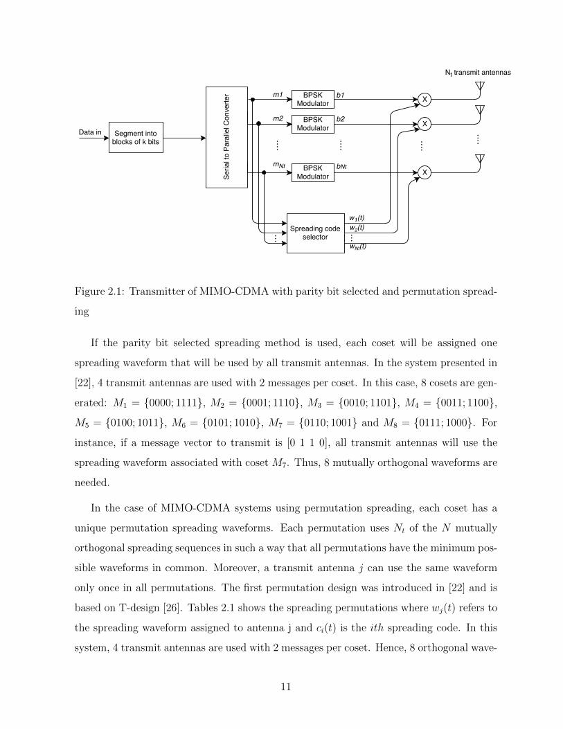
Figure 2.1: Transmitter of MIMO-CDMA with parity bit selected and permutation spread-
ing
If the parity bit selected spreading method is used, each coset will be assigned one
spreading waveform that will be used by all transmit antennas. In the system presented in
[22], 4 transmit antennas are used with 2 messages per coset. In this case, 8 cosets are gen-
erated: M1 = {0000; 1111}, M2 = {0001; 1110}, M3 = {0010; 1101}, M4 = {0011; 1100},
M5 = {0100; 1011}, M6 = {0101; 1010}, M7 = {0110; 1001} and M8 = {0111; 1000}. For
instance, if a message vector to transmit is [0 1 1 0], all transmit antennas will use the
spreading waveform associated with coset M7. Thus, 8 mutually orthogonal waveforms are
needed.
In the case of MIMO-CDMA systems using permutation spreading, each coset has a
unique permutation spreading waveforms. Each permutation uses Nt of the N mutually
orthogonal spreading sequences in such a way that all permutations have the minimum pos-
sible waveforms in common. Moreover, a transmit antenna j can use the same waveform
only once in all permutations. The first permutation design was introduced in [22] and is
based on T-design [26]. Tables 2.1 shows the spreading permutations where wj(t) refers to
the spreading waveform assigned to antenna j and ci(t) is the ith spreading code. In this
system, 4 transmit antennas are used with 2 messages per coset. Hence, 8 orthogonal wave-
11
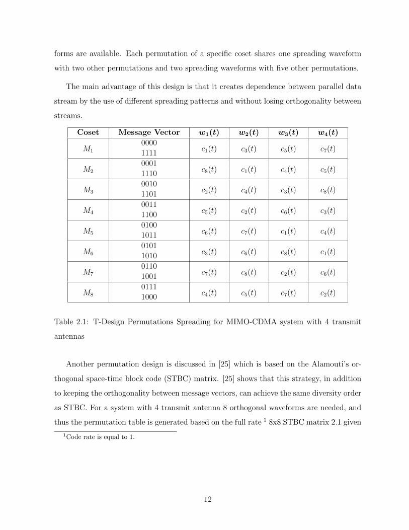
forms are available. Each permutation of a specific coset shares one spreading waveform
with two other permutations and two spreading waveforms with five other permutations.
The main advantage of this design is that it creates dependence between parallel data
stream by the use of different spreading patterns and without losing orthogonality between
streams.
Coset Message Vector w1(t) w2(t) w3(t) w4(t)
M1
0000c1(t) c3(t) c5(t) c7(t)1111
M2
0001c8(t) c1(t) c4(t) c5(t)1110
M3
0010c2(t) c4(t) c3(t) c8(t)1101
M4
0011c5(t) c2(t) c6(t) c3(t)1100
M5
0100c6(t) c7(t) c1(t) c4(t)1011
M6
0101c3(t) c6(t) c8(t) c1(t)1010
M7
0110c7(t) c8(t) c2(t) c6(t)1001
M8
0111c4(t) c5(t) c7(t) c2(t)1000
Table 2.1: T-Design Permutations Spreading for MIMO-CDMA system with 4 transmit
antennas
Another permutation design is discussed in [25] which is based on the Alamouti’s or-
thogonal space-time block code (STBC) matrix. [25] shows that this strategy, in addition
to keeping the orthogonality between message vectors, can achieve the same diversity order
as STBC. For a system with 4 transmit antenna 8 orthogonal waveforms are needed, and
thus the permutation table is generated based on the full rate 1 8x8 STBC matrix 2.1 given
1Code rate is equal to 1.
12

in [27].
s1 s2 s3 s4 s5 s6 s7 s8
−s2 s1 s4 −s3 s6 −s5 −s8 s7
−s3 s4 s1 s2 s7 s8 −s5 −s6−s4 s3 s2 s1 s8 −s7 s6 −s5−s5 s6 s7 −s8 s1 s2 s3 s4
−s6 s5 s8 s7 −s2 s1 −s4 s3
−s7 s8 s5 −s6 −s3 s4 s1 −s2−s8 s7 s6 s5 −s4 −s3 s2 s1
(2.1)
The spreading permutation table for 4 transmit antennas is given as follows 2:
Coset Message Vector w1(t) w2(t) w3(t) w4(t)
M1
0000c1(t) c5(t) c8(t) c6(t)1111
M2
0001c2(t) c6(t) c7(t) c5(t)1110
M3
0010c3(t) c7(t) c6(t) c8(t)1101
M4
0011c4(t) c8(t) c5(t) c7(t)1100
M5
0100c5(t) c1(t) c4(t) c2(t)1011
M6
0101c6(t) c2(t) c3(t) c1(t)1010
M7
0110c7(t) c3(t) c2(t) c4(t)1001
M8
0111c8(t) c4(t) c1(t) c3(t)1000
Table 2.2: STBC-Design Permutations Spreading for MIMO-CDMA system with 4 trans-
mit antennas
A more specific transmit signal table can be generated using the above concept. For
2Only 4 column from the 8x8 STBC matrix are needed to generate the permutations table. In [25]
column 1, 5, 8 and 6 are used. Other combination may be used as all columns in the STBC matrix are
orthogonal to each other.
13
example let us consider a MIMO-CDMA system with 4 transmit antennas using BPSK
modulation. If the message vector to be transmitted is m = [0 0 0 0] from coset M1, then
the transmit signal from antenna 1, 2,3 and 4 are given by:
m1 ∗ w1(t) = −c1(t)
m2 ∗ w2(t) = −c5(t)
m3 ∗ w3(t) = −c8(t)
m4 ∗ w4(t) = −c6(t)
(2.2)
where mj is the bit transmitted from the jth transmit antenna; and the wj(t) is the
spreading waveform assigned to antenna j.
Now, if the message vector to be transmitted is m = [1 1 1 1] from the same coset M1,
then the transmit signal from antenna 1, 2, 3 and 4 are given by:
m1 ∗ w1(t) = c1(t)
m2 ∗ w2(t) = c5(t)
m3 ∗ w3(t) = c8(t)
m4 ∗ w4(t) = c6(t)
(2.3)
The full transmit signals table is given as follows:
2.2.2 Receiver Model
Figure 2.2 shows the receiver block diagram of a MIMO-CDMA system using parity bit se-
lected and permutation spreading. Each receiver antenna is connected to a bank of matched
filters that corresponds to one of the N spreading waveform {c1(t), c2(t) . . . , cN(t)}. The
estimated transmitted bits are determined using the outputs of the matched filters as de-
cision variables and Maximum Likelihood (ML) as detection method [22]. Although the
receiver model looks to be similar for both techniques, the decision device is different.
Decision variable for MISO-CDMA system with Permutation Spreading
To determine the decision variable let us first consider a MISO-CDMA system with
parity bit selected spreading sequences using BPSK modulation with Nt transmit antennas
14

Coset Message Vector w1(t) w2(t) w3(t) w4(t)
M1
0000 c1(t) c5(t) c8(t) c6(t)
1111 −c1(t) −c5(t) −c8(t) −c6(t)
M2
0001 −c2(t) −c6(t) −c7(t) c5(t)
1110 c2(t) c6(t) c7(t) −c5(t)
M3
0010 −c3(t) −c7(t) c6(t) −c8(t)1101 c3(t) c7(t) −c6(t) c8(t)
M4
0011 −c4(t) −c8(t) c5(t) c7(t)
1100 c4(t) c8(t) −c5(t) −c7(t)
M5
0100 −c5(t) c1(t) −c4(t) −c2(t)1011 c5(t) −c1(t) c4(t) c2(t)
M6
0101 −c6(t) c2(t) −c3(t) c1(t)
1010 c6(t) −c2(t) c3(t) −c1(t)
M7
0110 −c7(t) c3(t) c2(t) −c4(t)1001 c7(t) −c3(t) −c2(t) c4(t)
M8
0111 −c8(t) c4(t) c1(t) c3(t)
1000 c8(t) −c4(t) −c1(t) −c3(t)
Table 2.3: STBC-Design Permutations Spreading transmit table for 4 transmit antennas
and 1 receive antenna. The received signal from a message vector (k), at each signalling
interval, is the sum of all bits multiplied by corresponding waveform and the channels gain
and it can be expressed as:
r(k)xparity bit=
Nt∑i=1
√Eb b
(k)i α
(k)1i w(k) + n(k) (2.4)
with Eb is the received energy per bit; α(k)1i is the complex channel gain between the ith
transmit antenna and the received antenna; b(k)i is the message bits transmitted over the ith
transmit antenna from the kthmessage vector; w(k) is the spreading sequence corresponding
to message vector k; n(k) is the receiver noise when receiving the kth message.
The output of the lth matched filter at the receive antenna during one signaling interval
is:
15
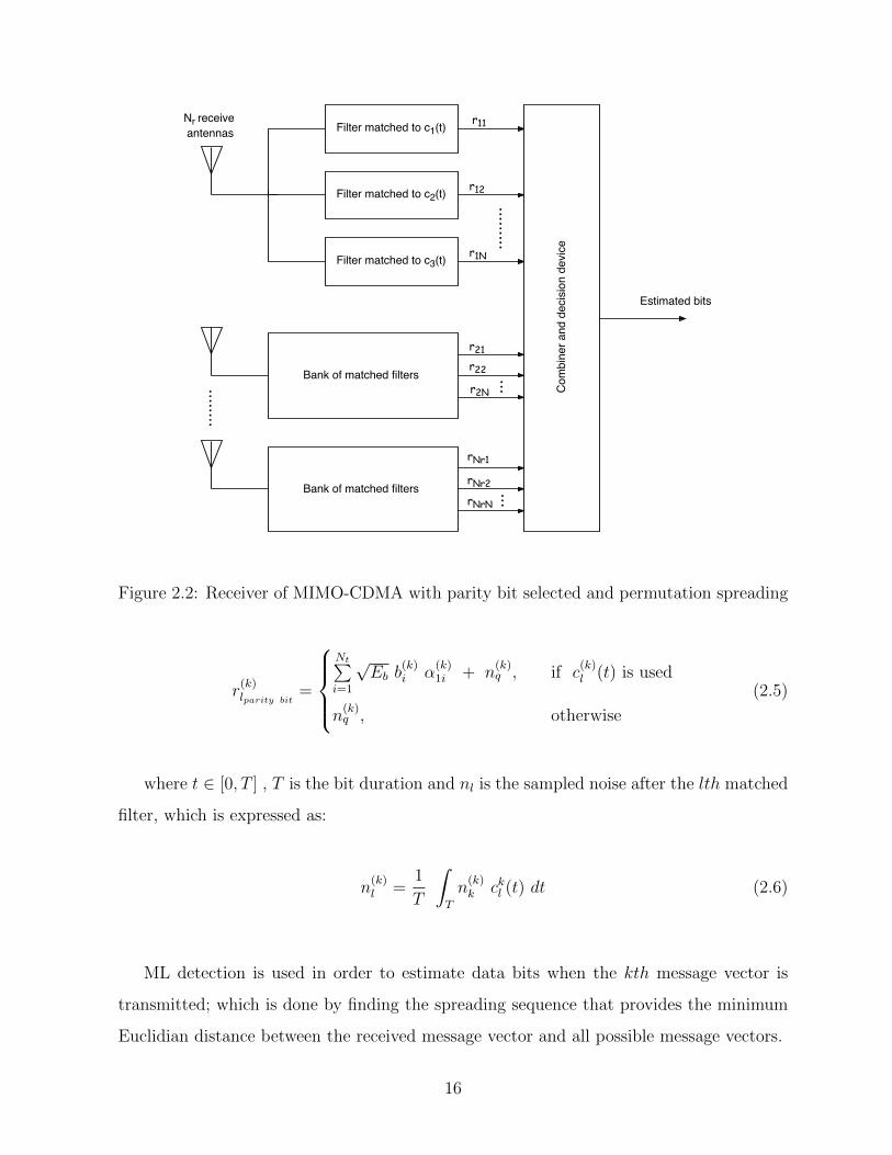
Figure 2.2: Receiver of MIMO-CDMA with parity bit selected and permutation spreading
r(k)lparity bit
=
Nt∑i=1
√Eb b
(k)i α
(k)1i + n
(k)q , if c
(k)l (t) is used
n(k)q , otherwise
(2.5)
where t ∈ [0, T ] , T is the bit duration and nl is the sampled noise after the lth matched
filter, which is expressed as:
n(k)l =
1
T
∫T
n(k)k ckl (t) dt (2.6)
ML detection is used in order to estimate data bits when the kth message vector is
transmitted; which is done by finding the spreading sequence that provides the minimum
Euclidian distance between the received message vector and all possible message vectors.
16

U =M
minj=1
∥∥∥∥∥r(k)xparity bit−
Nt∑i=1
√Eb b
(k)i α
(k)1i c
(k)i
∥∥∥∥∥2
(2.7)
where M is the total number of cosets.
Similarly, for MISO-CDMA system with permutation spreading the received message
vector can be expressed as:
r(k)xperm=
Nt∑i=1
√Eb b
(k)i α1i w
(k)i + n(k) (2.8)
with w(k)i is the spreading sequence assigned to the ith antenna when the kth message
vector is transmitted. The output of the lth matched filter at the receive antenna during
one time instant is:
r(k)lperm
=
Nt∑i=1
√Eb b
(k)i α
(k)1i + n
(k)q , if w
(k)i (t) = c
(k)i (t)
n(k)q , otherwise
(2.9)
In this case, the decision variable is expressed as follows:
U =M
minj=1
∥∥∥∥∥r(k)xperm−
Nt∑i=1
√Eb b
(k)i α
(k)1i w
(k)i
∥∥∥∥∥2
(2.10)
Decision variable for MIMO-CDMA system with Permutation Spreading
We notice that the decision variable is similar for both parity bit selected and per-
mutations spreading, except in the spreading sequence selection phase. For this reason,
only MIMO-CDMA system with permutation spreading sequences using BPSK modula-
tion with Nt transmit antennas and Nr receive antennas is considered in this section. The
17

output of the lth matched filter at the jth receive antenna during one signalling interval
is:
r(k)jl =
Nt∑i=1
√Eb
Nrb(k)i α
(k)ij + n
(k)jq , if w
(k)i (t) = c
(k)i (t)
n(k)jq , otherwise
(2.11)
with Eb is the received energy per bit; αij is the complex channel gain between the
ith transmit antenna and the jth received antenna; b(k)i is the ith message bits in the kth
message vector; wi is the spreading sequence corresponding to message vector k; n(k)jl is the
sampled noise after the lth matched at the jth receive antenna.
The received vector is expressed as follows:
rx = [r11, r12, . . . , r1N,r21, r22, . . . , r2N , . . . , rNr1, rNr2, . . . , rNrN ]T = ub + n (2.12)
where ub is the 1xN.Nr received data matrix that depends on the transmitted data
vector b = [b1, b2, . . . , bNt ]. For instance if the message to be transmitted, using the STBC-
design based on Table 2.3, is m = [1 1 1 0], then b = [1 1 1 − 1] and
ub = [0, α11, 0, 0,−α14, α12, α13, 0, . . . , 0, αNr1, 0, 0,−αNr4, αN−r2, αN−r3, 0]T .
n is the 1xN.Nr noise matrix n = [n11, . . . , n1N , n21, . . . , n2N , . . . , nNr1, .., nNrN ]T .
ML detection is used to estimate the data bits when the kth message vector is trans-
mitted. The expression of the decision variable is as follows:
U =M
minj=1 ‖rx − ub‖2 (2.13)
where ub is the vector made up of all possible received vector with the absence of the noise.
18

2.3 Theoretical analysis of the BER performance
2.3.1 BER analysis for MIMO-CDMA system with parity bit
selected spreading
In [28] an analytical expression is shown for the union bound of the BER for a MIMO-
CDMA system employing parity bit selected spreading. The BER is determined by inte-
grating the probability density function (pdf) of the energy per bit to noise power density
ratio (Eb/N0) multiplied by a Q-function. The pdf of Eb/N0 is shown, in [28], to be a
chi-square distribution with 2L degree of freedom for a MIMO system with Nt transmit
antenna and Nr receive antenna. The integration result has the form of the following
expression [29]:
p(L, x) =
(1− µ
2
)L L−1∑k=0
(L− 1 + k
k
) (1 + µ
2
)k
(2.14)
where
µ =
√x
x+ 1(2.15)
Study in [28] shows that the BER of a MIMO system employing parity bit selected
spreading sequence can be determined by, first, finding the squared Euclidian distance,
between constellation points, then computing the union bound of the BER. This holds
true under the following assumptions:
• Channels are assumed to be frequency-nonselective.
• Channel gains are independent, slowly varying and are known at the receiver.
• Maximum likelihood detection is used.
• Four transmit and received antennas and eight spreading waveforms are used.
19
Under these conditions, the union bound of the probability of bit for MIMO-CDMA
system employing parity bit selected spreading sequence is given by:
Pb = p1 + 4p2 + 3p3 (2.16)
with
p1 = p
(Nr,
4
Nr
Eb
N0
)(2.17)
p2 = p
(2Nr,
1
Nr
Eb
N0
)(2.18)
p3 =81
16p
(4,
3
8
Eb
N0
)+
1
16p
(4,
1
8
Eb
N0
)− 81
8p
(3,
3
8
Eb
N0
)+
3
8p
(3,
1
8
Eb
No
)+
405
32p
(2,
3
8
Eb
No
)+
405
32p
(1,
3
8
Eb
No
)+
45
32p
(2,
1
8
Eb
No
)− 135
32p
(1,
1
8
Eb
No
) (2.19)
2.3.2 BER analysis for MIMO-CDMA system with Permutation
Spreading
Same analysis of [28] is done in [22] to determine the union bound of the probability of bit
for a CDMA-MIMO system employing permutation spreading sequences based on STBC
design. The channels are assumed to be frequency non-selective with independent gains.
The bit error probability is determined by, first, finding the squared Euclidian distance,
between message vectors, then computing the union bound on the BER:
Pb = psame +
(M − 2
2
)pdiff (2.20)
where M is the number of message vectors and psame is the probability of error when
the receiver detects the correct spreading sequence but not the same data vector. psame is
given as follows:
psame = p
(NtNr,
1
Nr
Eb
N0
)(2.21)
20
pdiff is the probability of error when the receiver detects the incorrect spreading se-
quence. pdiff is given as follows:
pdiff = p
(NtNr,
1
2Nr
Eb
N0
)(2.22)
with p(L, x) is computed using equation 2.14.
2.4 Simulation results and discussion
Performance of the bit error rate (BER) of the three techniques discussed in this chapter is
presented in this section. All simulations are performed using Matlab where the following
assumption are considered:
• Orthogonal spreading codes are generated using Hadamard codes with length of 8
bits per chip sequence.
• All channel gains are considered to be independent, frequency non-selective and
slowly varying complex Gaussian random variables with zero means and unit vari-
ance.
• Perfect channel state information (CSI) is considered to be available at the receiver
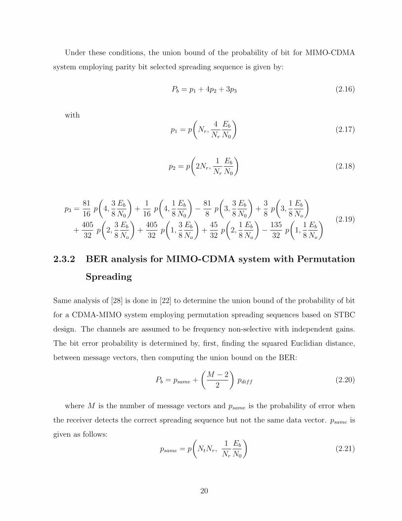
with zero power penalty.
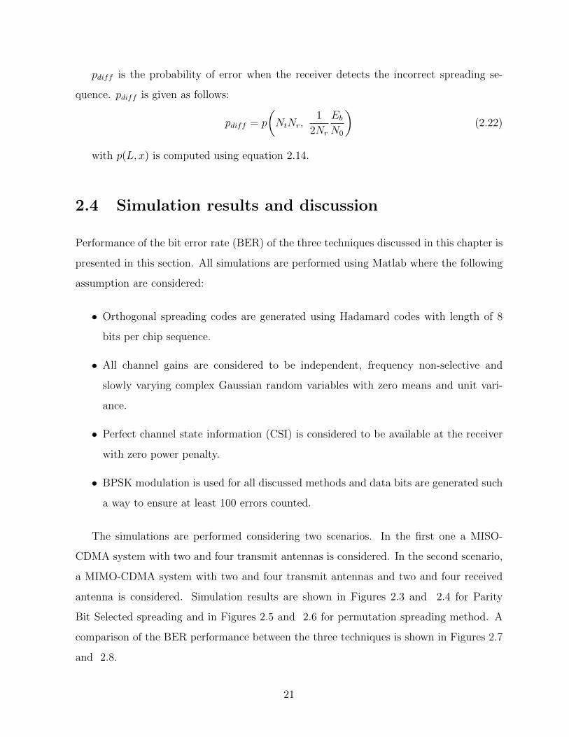
• BPSK modulation is used for all discussed methods and data bits are generated such
a way to ensure at least 100 errors counted.
The simulations are performed considering two scenarios. In the first one a MISO-
CDMA system with two and four transmit antennas is considered. In the second scenario,
a MIMO-CDMA system with two and four transmit antennas and two and four received
antenna is considered. Simulation results are shown in Figures 2.3 and 2.4 for Parity
Bit Selected spreading and in Figures 2.5 and 2.6 for permutation spreading method. A
comparison of the BER performance between the three techniques is shown in Figures 2.7
and 2.8.
21

0 2 4 6 8 10 12 14 16
Eb/No (dB)
10 -3
10 -2
10 -1
100
BE
R
Theoretical PB Spreading Nt=4Simulation PB Spreading Nt=4Theoretical PB Spreading Nt=2Simulation PB Spreading Nt=2
Figure 2.3: BER performance of MISO-CDMA System with parity bit selected spreading
Figure 2.4: BER performance of MIMO-CDMA System with parity bit selected spreading
22
Figure 2.5: BER performance of MISO-CDMA System with STBC permutation spreading
Figure 2.6: BER performance of MIMO-CDMA System with STBC permutation spreading
23

Figure 2.7: BER performance comparison of MISO-CDMA System using the three tech-
niques
Figure 2.8: BER performance comparison of MIMO-CDMA System using the three tech-
niques
24
2.4.1 Discussion
It can be seen from Figures 2.7 and 2.8 that permutation methods provide better BER
performance compared to the parity bit selected spreading technique. This is due to the
difference in the decision variables of each method. In the case of the parity bit selected
spreading, only one decision variable per antenna contains the sum of the transmitted
signals plus noise; all the other decision variables contain only noise. However, in per-
mutation spreading all decision variables contain one signal component plus noise or only
noise. Moreover, the permutation spreading using STBC design provides slightly improve-
ment in the bit error rate (BER) performance comparing to T-design without any increase
of the system complexity. This is due to the fact that the STBC design adds certain code
symmetry, which adds some degree of freedom in the Euclidean distance between constel-
lation points [25]. Finally, We can notice that the union bound estimation is close to the
simulation results and it is tight as the SNR increases. This is due because the union bound
estimation doesn’t include the probability of intersection events which tends towards zero
as the SNR increases.
25
Chapter 3
Spatial Modulation
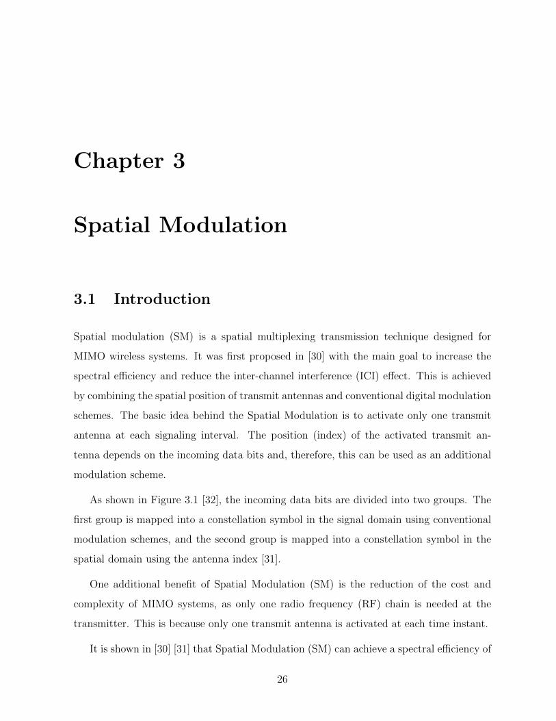
3.1 Introduction
Spatial modulation (SM) is a spatial multiplexing transmission technique designed for
MIMO wireless systems. It was first proposed in [30] with the main goal to increase the
spectral efficiency and reduce the inter-channel interference (ICI) effect. This is achieved
by combining the spatial position of transmit antennas and conventional digital modulation
schemes. The basic idea behind the Spatial Modulation is to activate only one transmit
antenna at each signaling interval. The position (index) of the activated transmit an-
tenna depends on the incoming data bits and, therefore, this can be used as an additional
modulation scheme.
As shown in Figure 3.1 [32], the incoming data bits are divided into two groups. The
first group is mapped into a constellation symbol in the signal domain using conventional
modulation schemes, and the second group is mapped into a constellation symbol in the
spatial domain using the antenna index [31].
One additional benefit of Spatial Modulation (SM) is the reduction of the cost and
complexity of MIMO systems, as only one radio frequency (RF) chain is needed at the
transmitter. This is because only one transmit antenna is activated at each time instant.
It is shown in [30] [31] that Spatial Modulation (SM) can achieve a spectral efficiency of
26

Signalconstellationforthefirsttransmitantenna
Signalconstellationforthelasttransmitantenna
Spatialconstellation
11–Ant_4
10–Ant_3
11–Ant_2
11–Ant_1
01(00) 00(00)
11(00)10(00)
01(11) 00(11)
11(11)10(11)
ImIm
Im
Im
Re
Re
Re
Re
Figure 3.1: SM constellation diagram
log2(Nt), where Nt is the number of transmit antennas, compared to V-BLAST. However,
this logarithmic increase will require a large number of available antennas 1. In order to
overcome this limitation, an extended technique called Generalized Spatial Modulation
(GSM) is proposed in [33] where more than one transmit antenna is activated at each
signaling interval. In GSM, data bits are mapped into different combinations of transmit
antennas at each time instant. Furthermore, GSM technique provides additional spatial
diversity gain, which improves the reliability of the communication channel.
Motivated by the above goal, various versions of Spatial Modulation (SM) were pro-
posed. In [34] a method based on Space Shift Keying (SSK) termed as General SSK
(GSSK) is presented where more than one antenna is activated at each signaling interval
and all data bits are mapped into the activated antennas. Hence, no signal constellation
is used. Simulations in [34] showed that GSSK requires less number of transmit antennas
to achieve the same performance as SM. Another technique called Fractional Bit Encoded
Spatial Modulation (FBE-SM) is proposed in [35] where the theory of modulus conversion
is used. In this case, an arbitrary number of transmit antennas can be used. One of the
1number of transmit antenna should be a power of two.
27
main drawbacks of this method is the error propagation. As discussed in [33], GSM is
proven to provide the same performance, with less required transmit antennas, as SM,
FBE-SM and GSSK. In this section, only the conventional SM and GSM methods are
discussed.
Figure 3.2 illustrates the difference between the concept of spatial modulation (SM),
Orthogonal Space Time Block Coding (OSTBC) and Spatial Multiplexing (SMX) [9].
It can be seen from Figure 3.2 that, in the case of SMX, the two symbols S1 and
S2 are transmitted at the same time instance using both antennas with a rate of Nt ∗
log2(M), where M is the modulation order and Nt is the number of transmit antennas. For
OSTBC, the two symbols are first encoded using Alamouti algorithm, then transmitted
in two signaling interval and using both transmit antennas. The data rate for OSTBC
is Nm/Ncu ∗ log2(M), where Ncu is the number of channel use and Nm is the number of
transmitted symbols. In the other hand, SM uses one symbol (S2) to select the transmit
antenna to activate and transmit the second symbol (S1) using this transmit antenna. The
data rate in this case is log2(Nt) + log2(M).
3.2 Spatial Modulation (SM) system model
The system model of the Spatial Modulation (SM) is shown in Figure 3.3 below where
4 transmit antennas and 4 received antennas are used [36]. In this system, BPSK is
considered for illustration purpose. Different constellation schemes and number of antennas
can, also, be used as described in details in [30].
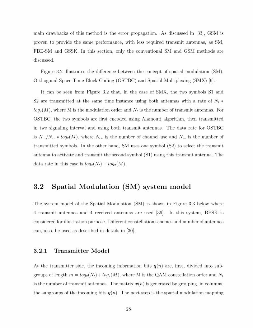
3.2.1 Transmitter Model
At the transmitter side, the incoming information bits q(n) are, first, divided into sub-
groups of length m = log2(Nt) + log2(M), where M is the QAM constellation order and Nt
is the number of transmit antennas. The matrix x(n) is generated by grouping, in columns,
the subgroups of the incoming bits q(n). The next step is the spatial modulation mapping
28
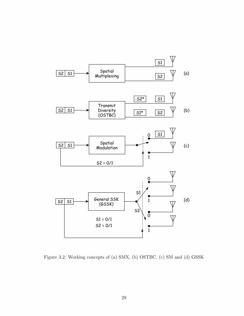
Figure 3.2: Working concepts of (a) SMX, (b) OSTBC, (c) SM and (d) GSSK
29

Figure 3.3: Spatial Modulation system model
where the vector x(n) is mapped to a new matrix s(n) using the mapping Table 3.1. As
shown in Figure 3.3, the matrix s(n) contains one nonzero element in each column which
is the symbol to transmit, at each time instance, using only one transmit antenna. An
example of this process is shown in Figure 3.3 for two time instants. At the first signaling
interval, the data to transmit is x(1) = [0 1 0]T that is mapped, using the mapping table,
to s(1) = [0 − 1 0 0]. In this case, only the second antenna will be active and will be
transmitting the symbol s = −1 and all other antennas will be silent.
Grouped
Bits
Antenna
IndexSymbol
000 1 −1
001 1 +1
010 2 −1
011 2 +1
100 3 −1
101 3 +1
110 4 −1
111 4 +1
Table 3.1: SM mapping table using BPSK and Nt=4
Other modulation scheme can be used in order to increase the data rate. For instance,
four transmit antennas with 4QAM modulation can be used to transmit 4 data bits as
shown in the mapping Table 3.2 below. In this example, the first two bits are used to
30
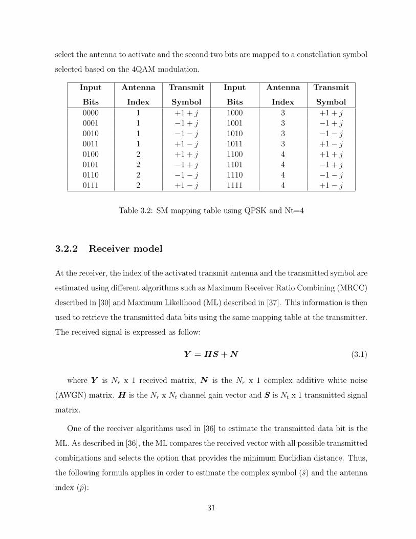
select the antenna to activate and the second two bits are mapped to a constellation symbol
selected based on the 4QAM modulation.
Input
Bits
Antenna
Index
Transmit
Symbol
Input
Bits
Antenna
Index
Transmit
Symbol
0000 1 +1 + j 1000 3 +1 + j
0001 1 −1 + j 1001 3 −1 + j
0010 1 −1− j 1010 3 −1− j0011 1 +1− j 1011 3 +1− j0100 2 +1 + j 1100 4 +1 + j
0101 2 −1 + j 1101 4 −1 + j
0110 2 −1− j 1110 4 −1− j0111 2 +1− j 1111 4 +1− j
Table 3.2: SM mapping table using QPSK and Nt=4
3.2.2 Receiver model
At the receiver, the index of the activated transmit antenna and the transmitted symbol are
estimated using different algorithms such as Maximum Receiver Ratio Combining (MRCC)
described in [30] and Maximum Likelihood (ML) described in [37]. This information is then
used to retrieve the transmitted data bits using the same mapping table at the transmitter.
The received signal is expressed as follow:
Y = HS + N (3.1)
where Y is Nr x 1 received matrix, N is the Nr x 1 complex additive white noise
(AWGN) matrix. H is the Nr x Nt channel gain vector and S is Nt x 1 transmitted signal
matrix.
One of the receiver algorithms used in [36] to estimate the transmitted data bit is the
ML. As described in [36], the ML compares the received vector with all possible transmitted
combinations and selects the option that provides the minimum Euclidian distance. Thus,
the following formula applies in order to estimate the complex symbol (s) and the antenna
index (p):
31

(p, s) = argminp,s
Nr∑i=1
‖yi −Hp,s.s‖2 (3.2)
where yi is the received vector at the ith received antenna when transmitting symbol s
and using the pth antenna with 1 ≤ p ≤ Nt and s ∈ {M}.
Equation 3.2 requires high computational complexity O(NtM(4Nr−1)), that increases
linearly with the number of transmit antennas. This is due because the receiver needs to
evaluate all possible combinations. To solve this issue a low-complexity detector, based
on Sphere Decoding (SD) and tree search structure, is proposed in [36]. The SD aims to
decrease the receiver computational complexity by applying ML detection over all points
that are inside a sphere of a specific radius C. The proposed algorithm combines the concept
of the conventional Sphere Decoder, described in [36], and the tree search structure in
order to avoid the main problem of having no point inside the sphere. Moreover, in this
new method the computational complexity of the points inside the sphere is less then the
conventional SD because only one transmit antenna is activated at each time instant[38].
The algorithm, first, sets an initial radius that depends on the noise level at the receiver
as given in 3.3. It, then, searches for any point that has a Euclidean distance less or equal
to the fixed radius C. Next, the algorithm updates the radius value by the Euclidean
distance of the founded point. Finally, the point with the minimum Euclidean distance is
considered to be the solution
C2 = 2 α Nr σ2n (3.3)
Where σ2n is the variance of the noise at the signaling interval n and α is a constant
used to maximize the possibility of having transmitted constellation point inside the used
sphere.
Simulations in [36] showed that the proposed Sphere Decoder (SD) could achieve the
same performance as the ML with a reduction of the computational complexity up to 85%.
32

3.3 Generalized Spatial Modulation (GSM) system
model
Generalized Spatial Modulation (GSM) was first introduced in [33] and it is an extension
of SM technique described in the pervious section. It was developed in order to overcome
the limitation of the logarithmic increase of the number of transmit antennas in SM. As
oppose to SM, in GSM more than one transmit antenna can be activated at each signaling
interval and the same complex symbol is transmitted over the activated transmit antennas.
Therefore, the antennas combinations are used as spatial constellation points to increase
the spectral efficiency. In GSM, the number of transmit antennas combinations that can
be used should be a power of two and the total number of possible combinations is(Nt
Na
),
where Na is the number of antenna to activate at each time instant and Nt is the number
of available transmit antennas. As discussed before, SM has a spectral gain of log2(Nt).
Whereas in GSM the spectral gain is blog2(Nt
Na
)c, where b.c is the floor operation. It
can be noticed that GSM has greater spectral gain than SM for the same number of
transmit antennas. Moreover, in Generalized Spatial Modulation the receiver receives
multiple copies of the transmitted symbol, which provides additional diversity gain.
The Generalized Spatial Modulation system model is shown in Figure 3.4 [33]. In this
example, 5 transmit antennas are used where only two can be activated at each signaling
interval.
3.3.1 Transmitter Model
The incoming data bits q(n) are, first, divided into subgroups of length m = ma + ms =
blog2(Nt
Na
)c+ log2(M). The first ma bits, of each subgroups, are used to select the transmit
antennas combination from Table 3.3. The next ms bits are modulated using any signal
modulations schemes such as M-QAM.
For example, it can be seen from Figure 3.4 that the data bits to be transmitted at the
first signaling interval are g(n) = [0 1 0 1]. The first three bits [0 1 0] are used to select a
33

Figure 3.4: Generalized Spatial Modulation system model
combination of transmit antenna from Table 3.3, which are antennas 1 and 4. Then, the last
bit {1} is modulated using BPSK, which is equivalent to a symbol s = +1. Therefore, the
corresponding column of the mapped vector at this time instant is x(n) = [+1 0 0 +1 0].
For the same example, if the SM is used, the required number of transmit antennas is equal
to eight in order to keep the same spectral efficiency.
Other modulation scheme can be used in order to increase the number of transmitted
bits. For instance, in the example shown in Table 3.3 the data bit can be increased to 5
bits by using QPSK modulation.
Motivated by the same concept of GSM, a modified version termed as Variable Gen-
eralized Spatial Modulation (VGSM) is proposed in [39] where the number of transmit
antennas to activate, at each signaling interval, varies from one transmit antenna to more
than one. The aim of this method is to increase the number of combinations that can be
used. In VGSM, the total number of possible combinations is expressed as follows:
ρV GSM =Nt∑i=1
(Nt
i
)= 2Nt − 1 (3.4)
Same as GSM, the number of possible combinations to use should be a power of two.
Therefore, the spectral efficiency is expressed as follows:
34
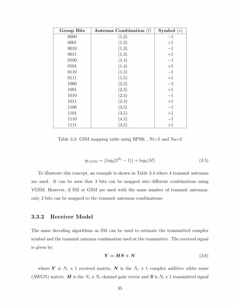
Group Bits Antenna Combination (l) Symbol (s)
0000 (1,2) −1
0001 (1,2) +1
0010 (1,3) −1
0011 (1,3) +1
0100 (1,4) −1
0101 (1,4) +1
0110 (1,5) −1
0111 (1,5) +1
1000 (2,3) −1
1001 (2,3) +1
1010 (2,4) −1
1011 (2,4) +1
1100 (3,5) −1
1101 (3,5) +1
1110 (4,5) −1
1111 (4,5) +1
Table 3.3: GSM mapping table using BPSK , Nt=5 and Na=2
ηV GSM = blog2(2Nt − 1)c+ log2(M) (3.5)
To illustrate this concept, an example is shown in Table 3.4 where 4 transmit antennas
are used. It can be seen that 3 bits can be mapped into different combinations using
VGSM. However, if SM or GSM are used with the same number of transmit antennas,
only 2 bits can be mapped to the transmit antennas combinations.
3.3.2 Receiver Model
The same decoding algorithms as SM can be used to estimate the transmitted complex
symbol and the transmit antenna combination used at the transmitter. The received signal
is given by:
Y = HS + N (3.6)
where Y is Nr x 1 received matrix, N is the Nr x 1 complex additive white noise
(AWGN) matrix. H is the Nr x Nt channel gain vector and S is Nt x 1 transmitted signal
35

Group Bits Antenna Combination (lV GSM)
000 (1)
001 (2)
010 (3)
011 (4)
100 (1,2)
101 (1,3)
110 (1,4)
111 (2,3)
Table 3.4: VGSM mapping table using Nt=4
matrix.
ML is used to estimate the complex symbol (s) and the spatial symbol (p) as follows:
(p, s) = argminp,s
Nr∑i=1
‖yi −Hp,s.s‖2 (3.7)
where yi is the received message at the ith received antenna when transmitting symbol
s and using the pth antenna with 1 ≤ p ≤ Nt and s ∈ {M}.
3.4 Receiver complexity
The receiver complexity can be computed based on the number of complex operations
needed by the detection algorithm. As discussed before, the evaluation of the decision
variable, for the spatial modulation using ML, in Equation 3.2 can be expressed as follows
[36]:
CSMML= Nt M (4Nr − 1) (3.8)
On the other hand, the GSM receiver complexity using ML can be expressed as follow
[33]:
CGSMML= Nr Nt M (Na + 2) (3.9)
The complexity ratio between these two techniques can be computed as follows:
36
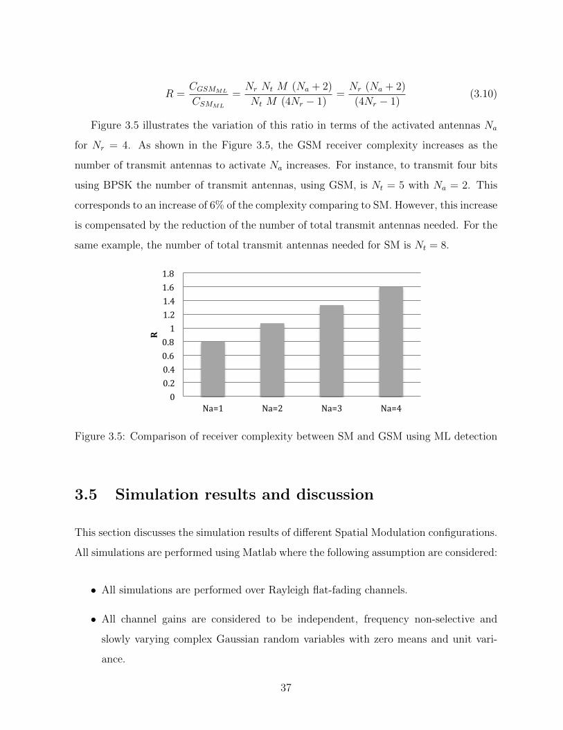
R =CGSMML
CSMML
=Nr Nt M (Na + 2)
Nt M (4Nr − 1)=Nr (Na + 2)
(4Nr − 1)(3.10)
Figure 3.5 illustrates the variation of this ratio in terms of the activated antennas Na
for Nr = 4. As shown in the Figure 3.5, the GSM receiver complexity increases as the
number of transmit antennas to activate Na increases. For instance, to transmit four bits
using BPSK the number of transmit antennas, using GSM, is Nt = 5 with Na = 2. This
corresponds to an increase of 6% of the complexity comparing to SM. However, this increase
is compensated by the reduction of the number of total transmit antennas needed. For the
same example, the number of total transmit antennas needed for SM is Nt = 8.
00.20.40.60.81
1.21.41.61.8
Na=1 Na=2 Na=3 Na=4
R
Signalconstellationforthefirsttransmitantenna
Signalconstellationforthelasttransmitantenna
Spatialconstellation
11–Ant_4
10–Ant_3
11–Ant_2
11–Ant_1
01(00) 00(00)
11(00)10(00)
01(11) 00(11)
11(11)10(11)
ImIm
Im
Im
Re
Re
Re
Re
Figure 3.5: Comparison of receiver complexity between SM and GSM using ML detection
3.5 Simulation results and discussion
This section discusses the simulation results of different Spatial Modulation configurations.
All simulations are performed using Matlab where the following assumption are considered:
• All simulations are performed over Rayleigh flat-fading channels.
• All channel gains are considered to be independent, frequency non-selective and
slowly varying complex Gaussian random variables with zero means and unit vari-
ance.
37

• Perfect channel state information (CSI) is considered to be available at the receiver
with zero power penalty.
• BPSK modulation is used for all discussed methods and data bits are generated such
a way to ensure at least 100 errors counted. All configurations have four receiver
antennas.
Three scenarios are considered in order to achieve a spectral efficiency of η = 4bits/s/Hz,
η = 6bits/s/Hz and η = 8bits/s/Hz. Figure 3.6 shows the BER performance using Spatial
Modulation of the three scenarios. It can be seen that as the number of bits to transmit
increases, the number of transmit antennas increases as well, which increase the complexity
and thus degrades the SM performance. In Figure 3.7 a comparison of BER performance
for η = 4bits/s/H is shown, where Nt = 8 for SM, Nt = 5 and Na = 2 for GSM and Nt = 4
for VGSM. The performances of the three techniques are close to each other with a slightly
better BER of SM at high SNR. However, GSM and VGSM require about half the number
of transmit antennas compared to SM. For η = 6bits/s/H results are shown in Figure 3.8,
where Nt = 32 for SM, Nt = 7 and Na = 3 for GSM and Nt = 6 for VGSM. Figure 3.9
illustrates results for η = 8bits/s/H, where Nt = 128 for SM, Nt = 12 and Na = 3 for
GSM and Nt = 8 for VGSM. Same observation can be noticed in both figures where SM
has slightly better performance at high SNR. Moreover, it can be seen that VGSM offers
slightly better results than GSM with less required transmit antennas.
In summary, GSM and VGSM can provide acceptable performance, comparing to SM,
with less number of transmit antennas and less complexity.
38
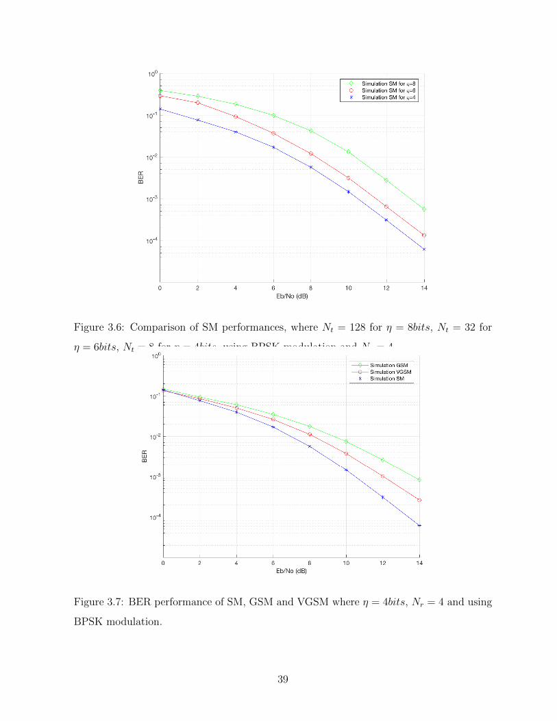
Figure 3.6: Comparison of SM performances, where Nt = 128 for η = 8bits, Nt = 32 for
η = 6bits, Nt = 8 for η = 4bits, using BPSK modulation and Nr = 4
Figure 3.7: BER performance of SM, GSM and VGSM where η = 4bits, Nr = 4 and using
BPSK modulation.
39

Figure 3.8: BER performance of SM, GSM and VGSM where η = 6bits, Nr = 4 and using
BPSK modulation.
Figure 3.9: BER performance of SM, GSM and VGSM where η = 8bits, Nr = 4 and using
BPSK modulation.
40

3.5.1 Discussion
This chapter introduced the concept of SM and how the spatial positions of transmit
antennas can be used as additional information that can increase the spectral efficiency
of MIMO systems. The chapter also discussed the generalized idea of Spatial Modulation
(GSM) where more than one transmit antennas can be activated to send same data at
each signaling interval. GSM aims to overcome the limitation of SM where a power of
two transmit antennas is needed. It also offers additional spatial diversity gain. Then, the
chapter introduced an extension method of GSM where the number of transmit antennas
to activate, at each signaling interval, varies from one transmit antenna to more than one.
This techniques provides higher number of transmit antennas combinations compared to
GSM. Finally, Simulation results showed that the performance of these three techniques is
close to each other with slightly better BER performance of SM. However, the VGSM and
GSM can achieve acceptable performance with less transmit antennas and less complexity
compared to SM.
41
Chapter 4
Single User Permutation Spreading
Employing Spatial Modulation for
MIMO-CDMA system
4.1 Introduction
The application of SM has been discussed in different studies and it has been shown that
it can increase the spectral efficiency while avoiding Inter-Channel Interference (ICI) [30].
Moreover, as explained in chapter 2, SM reduces the hardware system cost, complexity and
energy consumption by using less Radio Frequency (RF) chains compared to conventional
MIMO systems.
On other hand, the extension of parity bit selected spreading technique to MIMO-
CDMA systems which was introduced in [22] and discussed in chapter 2, shows that a
performance gain can be obtained when the selected spreading sequences depends on the
data that is to be transmitted. In this chapter we introduce, for the first time, a new
technique that combines the benefits of SM and MIMO-CDMA systems that use permuta-
tion spreading. Rather than activating all Nt transmit antennas at each signaling interval
in a MIMO-CDMA system employing parity bit selected or permutation spreading, only
Na transmit antennas are activated. Similar to SM concept, a combination of transmit
42
antenna is selected from the(Nt
Na
)available possibilities where the selected combination of
transmit antennas depends on which coset the messages to transmit comes from. By doing
so, a reduction of system complexity and Inter-Channel Interference effect can be achieved
while keeping a certain diversity order compared to SM.
As it is shown later in this chapter, a significant improvement in the performance of
MIMO-CDMA systems with permutation spreading can be achieved at low SNR values
when SM is implemented.
4.2 System Model
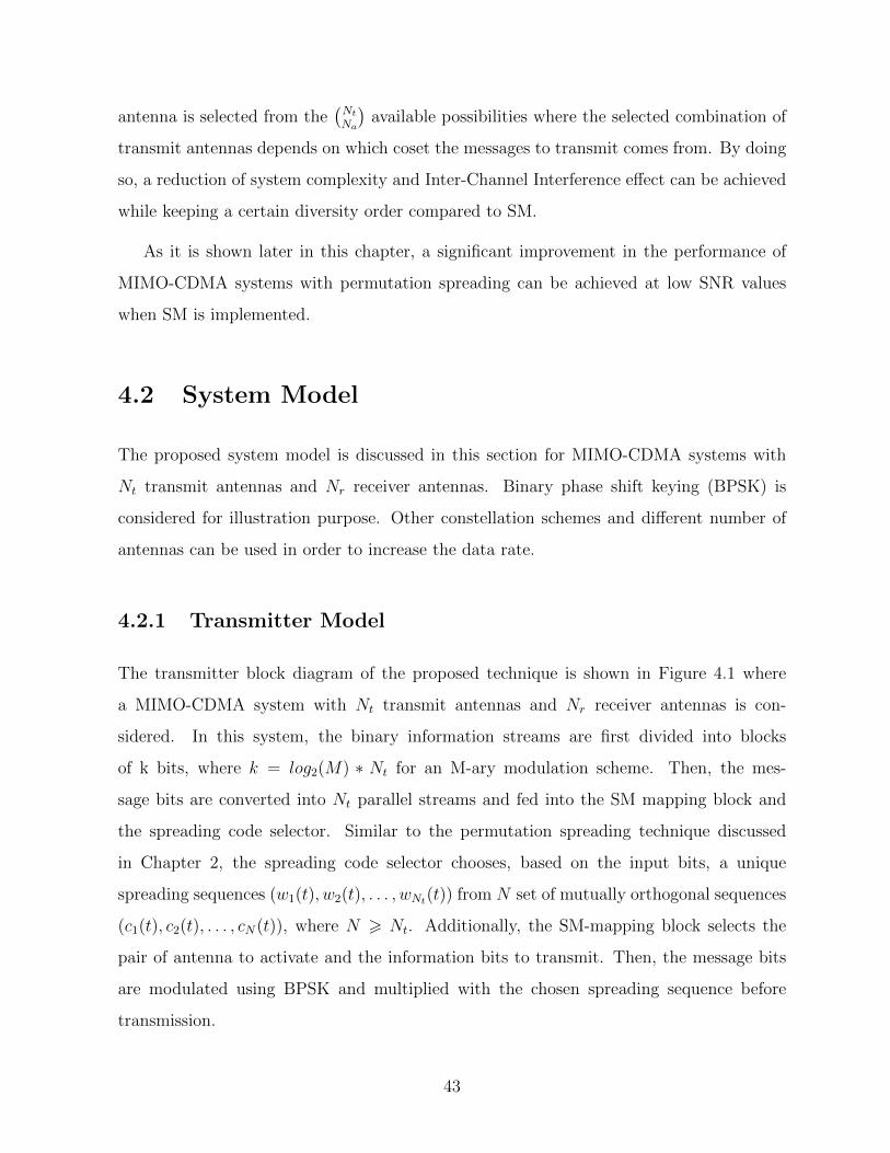
The proposed system model is discussed in this section for MIMO-CDMA systems with
Nt transmit antennas and Nr receiver antennas. Binary phase shift keying (BPSK) is
considered for illustration purpose. Other constellation schemes and different number of
antennas can be used in order to increase the data rate.
4.2.1 Transmitter Model
The transmitter block diagram of the proposed technique is shown in Figure 4.1 where
a MIMO-CDMA system with Nt transmit antennas and Nr receiver antennas is con-
sidered. In this system, the binary information streams are first divided into blocks
of k bits, where k = log2(M) ∗ Nt for an M-ary modulation scheme. Then, the mes-
sage bits are converted into Nt parallel streams and fed into the SM mapping block and
the spreading code selector. Similar to the permutation spreading technique discussed
in Chapter 2, the spreading code selector chooses, based on the input bits, a unique
spreading sequences (w1(t), w2(t), . . . , wNt(t)) from N set of mutually orthogonal sequences
(c1(t), c2(t), . . . , cN(t)), where N > Nt. Additionally, the SM-mapping block selects the
pair of antenna to activate and the information bits to transmit. Then, the message bits
are modulated using BPSK and multiplied with the chosen spreading sequence before
transmission.
43

Figure 4.1: The Transmitter of MIMO-CDMA with permutation spreading using SM
The design strategy is similar to the permutation spreading method discussed in [3,4]
and introduced in chapter 2, but with some modifications. In the spreading code selector
side, messages carried by the same spreading code are divided into cosets (M1,M2, . . . ,MK)
so that the Euclidian distance between messages in each coset is maximized. The number
of cosets (K) depends on the number of antennas (Nt) and the number of messages in each
coset (L): K = (2Nt)/L. Each coset will be assigned with a unique permutation spreading
waveforms. If the parity bit selected spreading method is used, each coset will have the
same spreading waveform that will be used by all transmit antennas.
The permutation design used is based on the Alamouti’s orthogonal STBC matrix in
order to preserve the orthogonality between message vectors and achieve a diversity order
similar to STBC as shown in [25]. For a system with 4 transmit antennas, 8 orthogonal
waveforms are needed, and thus the permutation table is generated based on the 8x8 STBC
matrix shown in 4.1. One of possible spreading permutation table for such system is given
as follows, where wj(t) refers to the spreading waveform assigned to antenna j and ci(t) is
the ith spreading code.
In the SM mapping block side, the message vector is divided into subgroups of length
m = ma +ms = blog2(Nt
Na
)c+ log2(M)∗Na, where Na is the number of transmit antenna to
activate at each time instant and Nt is the number of available transmit antennas. The first
44
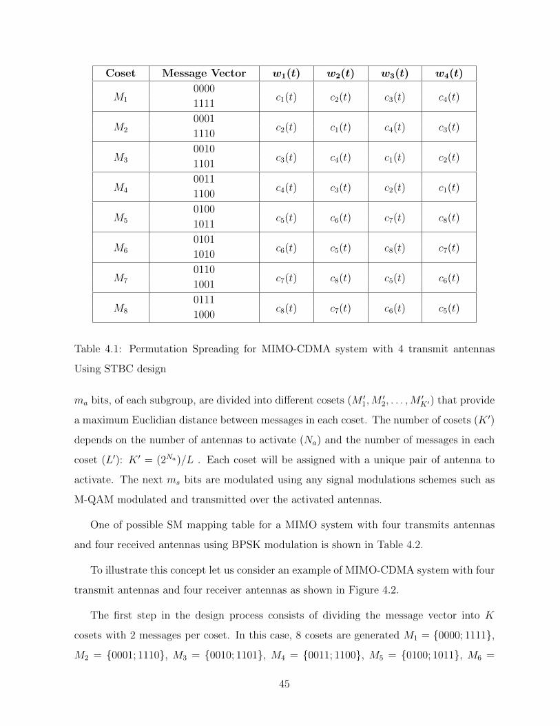
Coset Message Vector w1(t) w2(t) w3(t) w4(t)
M1
0000c1(t) c2(t) c3(t) c4(t)1111
M2
0001c2(t) c1(t) c4(t) c3(t)1110
M3
0010c3(t) c4(t) c1(t) c2(t)1101
M4
0011c4(t) c3(t) c2(t) c1(t)1100
M5
0100c5(t) c6(t) c7(t) c8(t)1011
M6
0101c6(t) c5(t) c8(t) c7(t)1010
M7
0110c7(t) c8(t) c5(t) c6(t)1001
M8
0111c8(t) c7(t) c6(t) c5(t)1000
Table 4.1: Permutation Spreading for MIMO-CDMA system with 4 transmit antennas
Using STBC design
ma bits, of each subgroup, are divided into different cosets (M ′1,M
′2, . . . ,M
′K′) that provide
a maximum Euclidian distance between messages in each coset. The number of cosets (K ′)
depends on the number of antennas to activate (Na) and the number of messages in each
coset (L′): K ′ = (2Na)/L . Each coset will be assigned with a unique pair of antenna to
activate. The next ms bits are modulated using any signal modulations schemes such as
M-QAM modulated and transmitted over the activated antennas.
One of possible SM mapping table for a MIMO system with four transmits antennas
and four received antennas using BPSK modulation is shown in Table 4.2.
To illustrate this concept let us consider an example of MIMO-CDMA system with four
transmit antennas and four receiver antennas as shown in Figure 4.2.
The first step in the design process consists of dividing the message vector into K
cosets with 2 messages per coset. In this case, 8 cosets are generated M1 = {0000; 1111},
M2 = {0001; 1110}, M3 = {0010; 1101}, M4 = {0011; 1100}, M5 = {0100; 1011}, M6 =
45
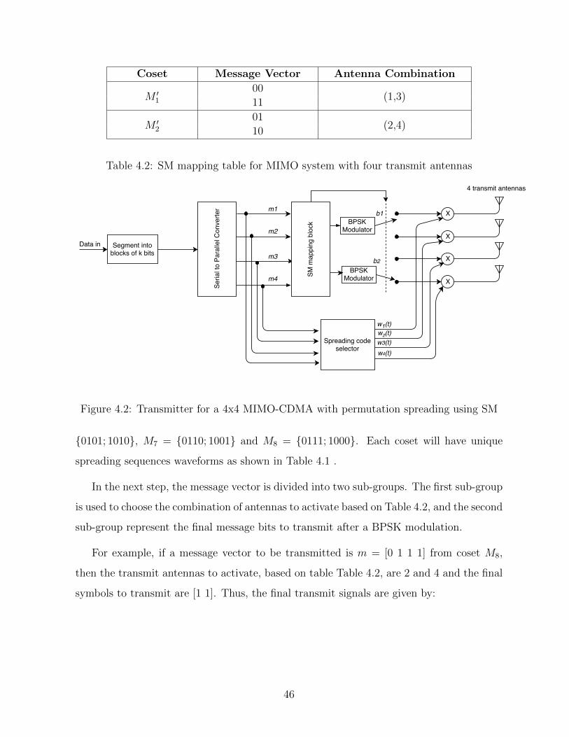
Coset Message Vector Antenna Combination
M ′1
00(1,3)
11
M ′2
01(2,4)
10
Table 4.2: SM mapping table for MIMO system with four transmit antennas
Figure 4.2: Transmitter for a 4x4 MIMO-CDMA with permutation spreading using SM
{0101; 1010}, M7 = {0110; 1001} and M8 = {0111; 1000}. Each coset will have unique
spreading sequences waveforms as shown in Table 4.1 .
In the next step, the message vector is divided into two sub-groups. The first sub-group
is used to choose the combination of antennas to activate based on Table 4.2, and the second
sub-group represent the final message bits to transmit after a BPSK modulation.
For example, if a message vector to be transmitted is m = [0 1 1 1] from coset M8,
then the transmit antennas to activate, based on table Table 4.2, are 2 and 4 and the final
symbols to transmit are [1 1]. Thus, the final transmit signals are given by:
46

Antenna1 Deactivated
Antenna2 s2 ∗ w2(t) = c7(t)
Antenna3 Deactivated
Antenna4 s4 ∗ w4(t) = c5(t)
(4.1)
where sj is the symbol transmitted from the jth antenna; and the wj(t) is the spreading
waveform assigned to antenna j.
Now, if the message vector to be transmitted is m = [1 1 0 0] from coset M4, then the
antennas to activate, based on Table 4.2, are 1 and 3 and the final symbols to transmit are
[−1 − 1]. Thus, the final transmit signals are given by:
Antenna1 s1 ∗ w1(t) = −c4(t)
Antenna2 Deactivated
Antenna3 s3 ∗ w3(t) = −c2(t)
Antenna4 Deactivated
(4.2)
The same idea can be applied to the parity bit selected spreading sequence where the
only difference is that the transmit antennas use the same waveform at each signaling
interval.
Table 4.3 shows the full transmit signal table for the system shown in Figure 4.2 using
BPSK modulation.
4.2.2 Receiver Model
The proposed receiver model is shown in Figure 4.3. Similar to the permutation spreading
sequences, each receiver antenna is equipped with a bank of matched filters that correspond
to one of the N spreading waveforms (c1(t), c2(t), . . . , cN(t)). The receiver estimates the
transmitted symbols and the index of the activated transit antennas using the ML and
the output of the matched filters as decision variables. The ML compares the received
vector with all possible transmitted combinations and selects the option that provides the
47
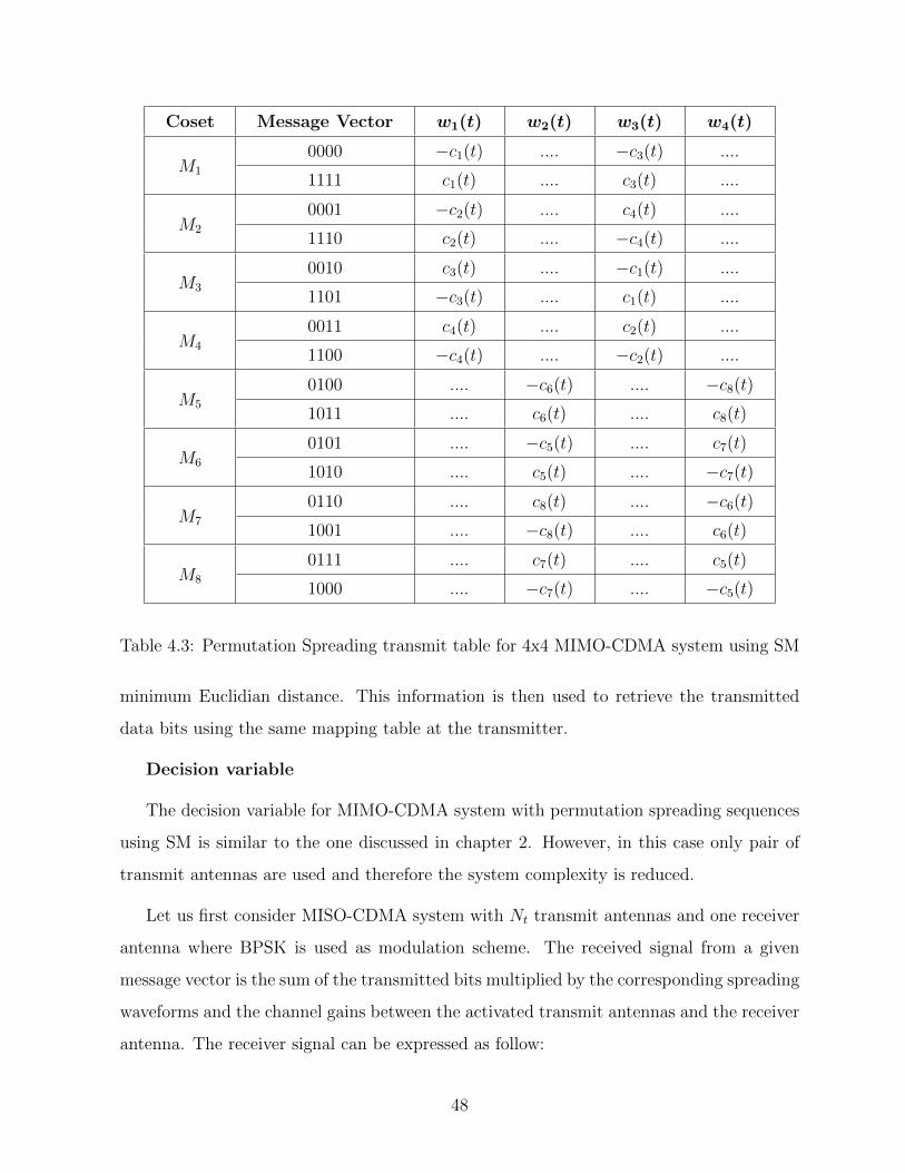
Coset Message Vector w1(t) w2(t) w3(t) w4(t)
M1
0000 −c1(t) .... −c3(t) ....
1111 c1(t) .... c3(t) ....
M2
0001 −c2(t) .... c4(t) ....
1110 c2(t) .... −c4(t) ....
M3
0010 c3(t) .... −c1(t) ....
1101 −c3(t) .... c1(t) ....
M4
0011 c4(t) .... c2(t) ....
1100 −c4(t) .... −c2(t) ....
M5
0100 .... −c6(t) .... −c8(t)1011 .... c6(t) .... c8(t)
M6
0101 .... −c5(t) .... c7(t)
1010 .... c5(t) .... −c7(t)
M7
0110 .... c8(t) .... −c6(t)1001 .... −c8(t) .... c6(t)
M8
0111 .... c7(t) .... c5(t)
1000 .... −c7(t) .... −c5(t)
Table 4.3: Permutation Spreading transmit table for 4x4 MIMO-CDMA system using SM
minimum Euclidian distance. This information is then used to retrieve the transmitted
data bits using the same mapping table at the transmitter.
Decision variable
The decision variable for MIMO-CDMA system with permutation spreading sequences
using SM is similar to the one discussed in chapter 2. However, in this case only pair of
transmit antennas are used and therefore the system complexity is reduced.
Let us first consider MISO-CDMA system with Nt transmit antennas and one receiver
antenna where BPSK is used as modulation scheme. The received signal from a given
message vector is the sum of the transmitted bits multiplied by the corresponding spreading
waveforms and the channel gains between the activated transmit antennas and the receiver
antenna. The receiver signal can be expressed as follow:
48

Figure 4.3: Receiver of MIMO/CDMA with permutation spreading using SM
r(k)x =Nt∑i=1
√Eb b
(k)i α
(k)1i w
(k)i + n(k) (4.3)
with Eb is the received energy per bit; α(k)1i is the complex channel gain between the
ith transmit antenna and the received antenna; b(k)i is the message bits transmitted over
the ith transmit antenna from the kth message vector; w(k)i is the spreading sequence used
by the ith transmit antenna and corresponding to kth message vector. n(k) is the receiver
noise when receiving the kth message.
As mentioned before in this section, only some of the transmit antennas will be active
at each signaling interval. Thus b(k)i in Formula 4.3 can either be equal to {0} if the
corresponding antenna is not used, or {−1} or {1}, depending on the message bit to
transmit, if the corresponding antenna is used.
49

The output of the lth matched filter at the receive antenna when transmitting the kth
message vector is:
r(k)l =
Nt∑i=1
√Eb b
(k)i α
(k)1i + n
(k)l , if c
(k)l (t) is used
n(k)l , otherwise
(4.4)
where n(k)l is the sampled noise after the lth matched filter when transmitting the kth
message vector.
ML detection is then used in order to estimate transmit antenna index (p) and data
bits (b) when the kth message vector is transmitted; this is done by finding the spreading
sequence that provides the minimum Euclidian distance between the received message
vector and all possible message vectors. Therefore, the decision variable for MISO-CDMA
system with permutation spreading sequences using SM is given as follows:
(p, b) =M
minj=1
∥∥∥∥∥r(k)x −Nt∑i=1
√Eb b
(k)i α
(k)1i w
(k)i
∥∥∥∥∥2
(4.5)
where M is the total number of cosets.
Now let us consider a MIMO-CDMA system with permutation spreading sequences
using SM with Nt transmit antenna and Nr receiver antenna. The received vector is
expressed as follows:
rx = [r11, r12, . . . , r1N , r21, r22, . . . , r2N , . . . , rNr1, rNr2, . . . , rNrN ]T (4.6)
where rjl is the output from the lth matched filter of the jth receiver antenna and it is
expressed as follows:
r(k)jl =
Nt∑i=1
√Eb
Nrb(k)i α
(k)ij + n
(k)jl , if c
(k)l is used
n(k)jl , otherwise
(4.7)
50

where α(k)ij is the complex channel gain between the ith transmit antenna and the jth
receiver antenna when transmitting message (k), and n(k)jl is the sampled noise after the
lth matched filter of the jth receiver antenna when message (k) is transmitted.
After the output of the matched filter, the received vector would be given as:
rx = ub + n (4.8)
where n is the 1xN.Nr noise matrix: n = [n11, . . . , n1N , n21, . . . , n2N , . . . , nNr1, .., nNrN ]T
and ub is the 1xN.Nr received data matrix that depends on the transmitted data vector
b = [b1, b2, . . . , bNt ].
For instance, if the message to be transmitted is m = [1 0 1 1], which is from coset
M5 according to Table 4.3. In this coset, antennas 2 and 4 are used and the last two
bits of the message m are to transmit. Then the data vector is b = [0 1 0 1] and ub =
[0, 0, 0, 0, 0, α12, 0, α14, 0, 0, 0, 0, 0, α22, 0, α24, . . . , 0, 0, 0, 0, 0, αNr2, 0, αNr4]T .
Now, if the message to be transmitted is m = [1 1 0 1], which is from coset M3
according to Table 4.3. In this coset, antennas 1 and 3 are used and the last two bits
of the message m are to transmit. Then the data vector is b = [−1 0 1 0] and ub =
[α13, 0,−α11, 0, 0, 0, 0, 0, α23, 0,−α21, 0, 0, 0, 0, 0, . . . , αNr3, 0, αNr1, 0, 0, 0, 0, 0]T .
ML detection is then used in order to estimate transmit antenna index (p) and data bits
(b) when the kth message vector is transmitted. Thus, the decision variable for MIMO-
CDMA system with permutation spreading sequences using SM is given by:
(p, b) =M
minj=1 ‖rx − ub‖2 (4.9)
where ub is the vector made up of all possible received vector with the absence of the
noise.
51
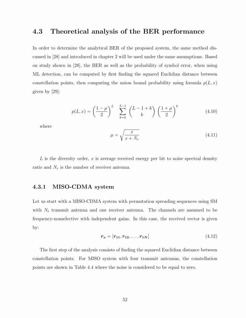
4.3 Theoretical analysis of the BER performance
In order to determine the analytical BER of the proposed system, the same method dis-
cussed in [28] and introduced in chapter 2 will be used under the same assumptions. Based
on study shown in [28], the BER as well as the probability of symbol error, when using
ML detection, can be computed by first finding the squared Euclidian distance between
constellation points, then computing the union bound probability using formula p(L, x)
given by [29]:
p(L, x) =
(1− µ
2
)L L−1∑k=0
(L− 1 + k
k
) (1 + µ
2
)k
(4.10)
where
µ =
√x
x+Nr
(4.11)
L is the diversity order, x is average received energy per bit to noise spectral density
ratio and Nr is the number of receiver antenna.
4.3.1 MISO-CDMA system
Let us start with a MISO-CDMA system with permutation spreading sequences using SM
with Nt transmit antenna and one receiver antenna. The channels are assumed to be
frequency-nonselective with independent gains. In this case, the received vector is given
by:
rx = [r11, r12, . . . , r1N ] (4.12)
The first step of the analysis consists of finding the squared Euclidian distance between
constellation points. For MISO system with four transmit antennas, the constellation
points are shown in Table 4.4 where the noise is considered to be equal to zero.
52
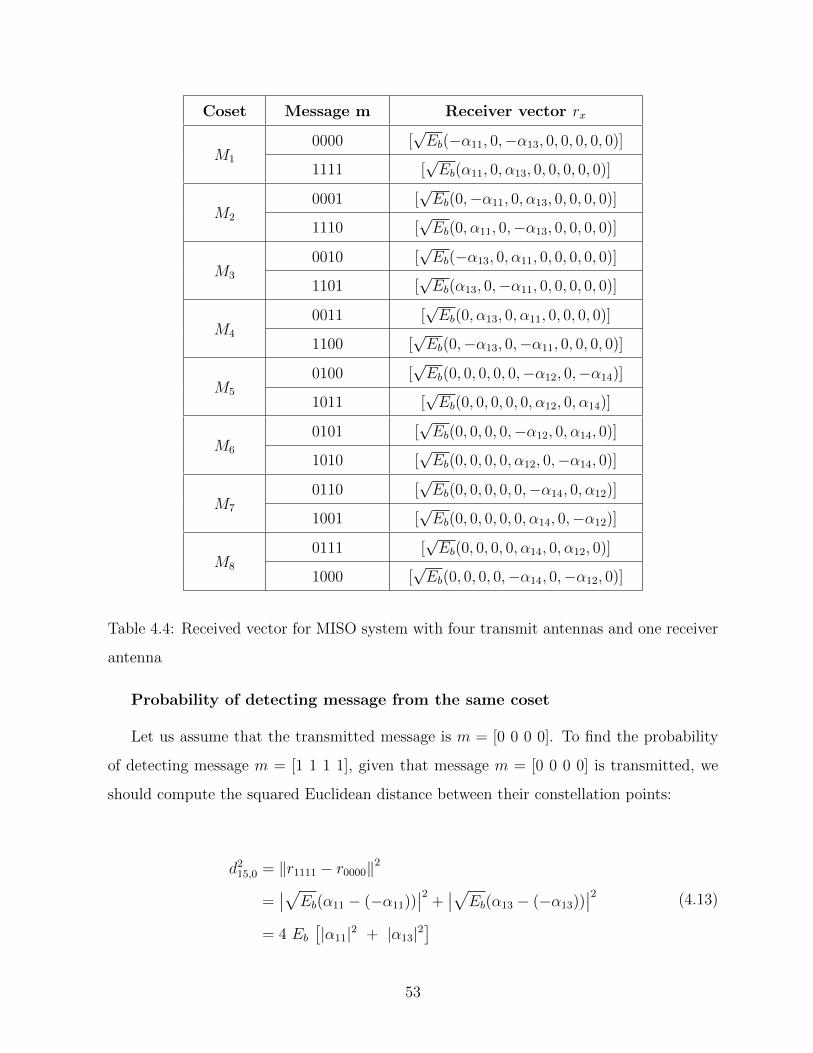
Coset Message m Receiver vector rx
M1
0000 [√Eb(−α11, 0,−α13, 0, 0, 0, 0, 0)]
1111 [√Eb(α11, 0, α13, 0, 0, 0, 0, 0)]
M2
0001 [√Eb(0,−α11, 0, α13, 0, 0, 0, 0)]
1110 [√Eb(0, α11, 0,−α13, 0, 0, 0, 0)]
M3
0010 [√Eb(−α13, 0, α11, 0, 0, 0, 0, 0)]
1101 [√Eb(α13, 0,−α11, 0, 0, 0, 0, 0)]
M4
0011 [√Eb(0, α13, 0, α11, 0, 0, 0, 0)]
1100 [√Eb(0,−α13, 0,−α11, 0, 0, 0, 0)]
M5
0100 [√Eb(0, 0, 0, 0, 0,−α12, 0,−α14)]
1011 [√Eb(0, 0, 0, 0, 0, α12, 0, α14)]
M6
0101 [√Eb(0, 0, 0, 0,−α12, 0, α14, 0)]
1010 [√Eb(0, 0, 0, 0, α12, 0,−α14, 0)]
M7
0110 [√Eb(0, 0, 0, 0, 0,−α14, 0, α12)]
1001 [√Eb(0, 0, 0, 0, 0, α14, 0,−α12)]
M8
0111 [√Eb(0, 0, 0, 0, α14, 0, α12, 0)]
1000 [√Eb(0, 0, 0, 0,−α14, 0,−α12, 0)]
Table 4.4: Received vector for MISO system with four transmit antennas and one receiver
antenna
Probability of detecting message from the same coset
Let us assume that the transmitted message is m = [0 0 0 0]. To find the probability
of detecting message m = [1 1 1 1], given that message m = [0 0 0 0] is transmitted, we
should compute the squared Euclidean distance between their constellation points:
d215,0 = ‖r1111 − r0000‖2
=∣∣√Eb(α11 − (−α11))
∣∣2 +∣∣√Eb(α13 − (−α13))
∣∣2= 4 Eb
[|α11|2 + |α13|2
] (4.13)
53

Similar to study shown in [28], it can be shown that d2(15,0) has a chi-square distribution
with 4 degree of freedom and diversity order of 2. Therefore, the probability that the
message m = [1 1 1 1] is detected given that message m = [0 0 0 0] is transmitted is given
by [29]:
p15 = p(2, 4γb) (4.14)
where γb is the average received SNR per bit.
Probability of detecting message from different coset but having the same
antenna index
In this section we investigate the probability that the receiver detects a different message
that uses the same set of transmit antennas. From Table 4.4, it can be seen that three
cosets (M2,M3 and M4) use the same transmit antenna combination. It can be shown that
all message vectors from these cosets have the same Euclidean distance and therefore the
same probability of error. We refer to this probability as pSame index.
Let us use message m = [1 1 0 0] from coset M4 as an example. The distance between
the constellation points of this message and message m = [0 0 0 0] is shown as follows:
d212,0 = ‖r1100 − r0000‖2
=∣∣√Eb α11
∣∣2 +∣∣√Eb α11
∣∣2 +∣∣√Eb α13
∣∣2 +∣∣√Eb α13
∣∣2= 2 Eb
[|α11|2 + |α13|2
] (4.15)
It can be shown that d212,0 has a chi-square distribution with 4 degree of freedom and
diversity order of 2. Therefore, the probability that the message m = [1 1 0 0] is detected
given that message m = [0 0 0 0] is transmitted is given as follows:
pSame index = p(2, 2γb) (4.16)
54

Probability of detecting message from different coset with different antenna
index
The last case of this analysis is when the receiver incorrectly detects a message from
a different coset that uses a different transmit antenna combination than the transmitted
message. From Table 4.4, it can be seen that the messages of four cosets (M5,M6,M7 and
M8) use a different transmit antenna combination than message m = [0 0 0 0]. It can be
shown that all message vectors from these cosets have the same Euclidean distance and
therefore the same probability of error. We refer to this probability as pDiff index.
Let us use message m = [1 0 0 0] from coset M8 as example. The distance between the
constellation points of this message and message m = [0 0 0 0] is shown as follows:
d28,0 = ‖r1000 − r0000‖2
=∣∣√Eb α11
∣∣2 +∣∣√Eb α13
∣∣2 +∣∣√Eb α12
∣∣2 +∣∣√Eb α14
∣∣2= Eb
[|α11|2 + |α12|2 + |α13|2 + + |α14|2
] (4.17)
It can be shown that d212,0 has a chi-square distribution with 8 degree of freedom and
diversity order of 4. Therefore, the probability that the message m = [1 0 0 0] is detected
given that message m = [0 0 0 0] is transmitted is given as follows:
pDiff index = p(4, γb) (4.18)
To estimate the probability of error detection when messagem = [0 0 0 0] is transmitted,
the union bound can be used [29]:
P (E | [0 0 0 0] <15∑i=1
pi|0
< p15 + 6 ∗ pSame index + 8 ∗ pDiff index
< p(2, 4γb) + 6 ∗ p(2, 2γb) + 8 ∗ p(4, γb)
(4.19)
55

As the probability of error detection is independent of the transmitted message [28], we
can write that P (E) = P (E|[0000]). Likewise, the probability of bit error is independent of
the message that has been sent; the union bound probability can be expressed as follows:
pb < p(2, 4γb) + 3 ∗ p(2, 2γb) + 4 ∗ p(4, γb) (4.20)
with p(L, x) is computed using Equation 4.10.
4.3.2 MIMO-CDMA system
Now let us consider MIMO-CDMA system with permutation spreading sequences using
SM with Nt transmit antennas and Nr receiver antennas. Under the same assumptions as
section 4.3.1, the received vector is given by:
rx = [r11, r12, . . . , r1N , r21, r22, . . . , r2N , . . . , rNr1, rNr2, . . . , rNrN ] (4.21)
For instance, if the transmitted message is m = [0 0 0 0], the received vector is shown
as:
r[0 0 0 0] =[√Eb
Nr
(− α11, 0,−α13, 0, 0, 0, 0, 0, . . . ,−αNr1, 0,−αNr3, 0, 0, 0, 0, 0
](4.22)
Following the same steps as the previous section, the probability of detecting message
m = [1 1 1 1], given that message m = [0 0 0 0] was transmitted is given as follows:
p15 = p(2Nr, 4γb) (4.23)
Similarly, the probability of detecting messages coming from different cosets but having
the same transmit antenna index is:
pSame index = p(2Nr, 2γb) (4.24)
56
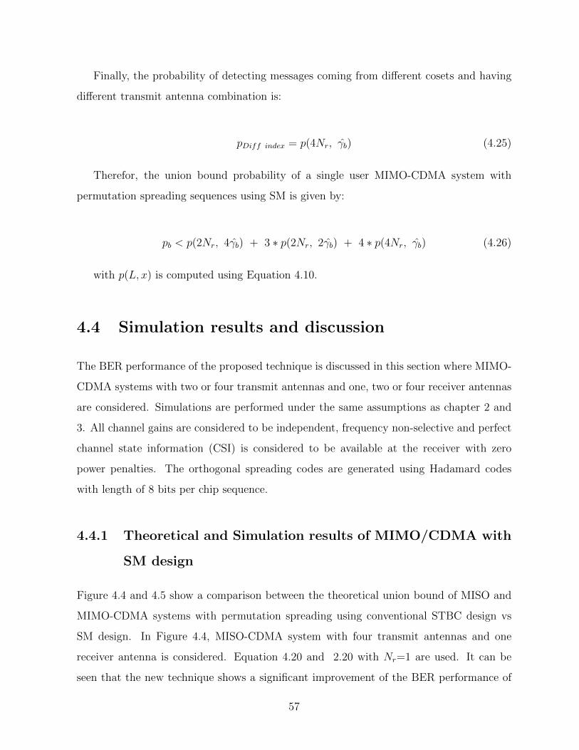
Finally, the probability of detecting messages coming from different cosets and having
different transmit antenna combination is:
pDiff index = p(4Nr, γb) (4.25)
Therefor, the union bound probability of a single user MIMO-CDMA system with
permutation spreading sequences using SM is given by:
pb < p(2Nr, 4γb) + 3 ∗ p(2Nr, 2γb) + 4 ∗ p(4Nr, γb) (4.26)
with p(L, x) is computed using Equation 4.10.
4.4 Simulation results and discussion
The BER performance of the proposed technique is discussed in this section where MIMO-
CDMA systems with two or four transmit antennas and one, two or four receiver antennas
are considered. Simulations are performed under the same assumptions as chapter 2 and
3. All channel gains are considered to be independent, frequency non-selective and perfect
channel state information (CSI) is considered to be available at the receiver with zero
power penalties. The orthogonal spreading codes are generated using Hadamard codes
with length of 8 bits per chip sequence.
4.4.1 Theoretical and Simulation results of MIMO/CDMA with
SM design
Figure 4.4 and 4.5 show a comparison between the theoretical union bound of MISO and
MIMO-CDMA systems with permutation spreading using conventional STBC design vs
SM design. In Figure 4.4, MISO-CDMA system with four transmit antennas and one
receiver antenna is considered. Equation 4.20 and 2.20 with Nr=1 are used. It can be
seen that the new technique shows a significant improvement of the BER performance of
57

about 2dB for an SNR between 0 and 4dB. This is due mainly to the fact of using less
transmit antennas and therefore reducing the inter-channel interferences. However, using
fewer antennas means less diversity gain. This can be noticed from Figure 4.4 where the
BER performance starts to drop for an SNR higher than 6dB.
In Figure 4.5 a MIMO-CDMA system with four transmit antennas and four receiver
antennas is considered. Formulas 4.26 and 2.20 with Nr = 4 are used. Same remarks as
Figure 4.5 can be observed, the performance is significantly improved for an SNR between
0 and 10dB. Since this system uses more transmit antennas, we can notice the additional
diversity gain effect where the BER performance starts to drop after an SNR of 12dB
compared to 8dB for the MISO system shown in Figure 4.5.
Figure 4.6 presents the simulation vs, theoretical results of the BER performance of
the proposed technique in MIMO-CDMA systems with 4 and 2 transmit antenna and 1,
2 and 4 receiver antennas. As expected, we can notice that the union bound estimation
derived in the previous section is close to the simulation results and it is tight as the SNR
increases. This is due because the union bound estimation doesn’t include the probability
of intersection events which tends towards zero as the SNR increases. We also notice
additional diversity gain as the number of antennas increases which improves the BER
performances.
4.4.2 Comparison of simulation results
In this section we compare the simulated results of the proposed technique and the con-
ventional STBC design and the conventional SM design.
Figure 4.7, 4.8 and 4.9 show, respectively, the simulated BER performances of the dif-
ferent techniques for 2 and 4 transmit antennas with 1, 2 and 4 receive antennas. It can be
seen that the new SM design provides a significant improvement of the BER performance,
of about 2 dB for 4x4 MIMO system, compared to the conventional STBC technique. Also,
we can notice that the BER performance start to drop as the SNR increases. However,
an important increase of the BER performance can be noticed as the number of antennas
increases.
58

Figure 4.4: Theoretical BER performance of 4x1 MISO-CDMA System using Permutation
Spreading with conventional STBC design vs SM design
Figure 4.5: Theoretical BER performance of 4x4 MIMO-CDMA System using Permutation
Spreading with conventional STBC design vs SM design
59
Figure 4.6: BER performance of MIMO-CDMA System with Permutation Spreading using
SM design
Figure 4.9 shows simulation performance of MIMO systems with spectral efficiency of
η = 4bits/s/Hz using the conventional SM techniques discussed in Chapter 2 and the new
SM permutation spreading proposed in this chapter. The number of transmit antennas are
set in order to achieve this spectral efficiency. Thus, For the conventional SM techniques
Nr = 4 and Nt = 8 for SM, Nt = 5 and Na = 2 for GSM and Nt = 4 for VGSM; where for
the proposed technique Nt = 4 and Nr = 4. We have to note that the new design uses 8
bits, for the spreading code, to transmit one bit at each time instant, whereas in SM only
one bit is transmitted at each signaling. However, as it will be shown in Chapter 5, the
simulation results show that when CDMA with SM permutation spreading is used a slightly
significant BER performance gain is achieved. This improvement is achieved because the
used design creates dependency between parallel bits and spreading waveforms in addition
to the dependency between bits and antenna combinations.
60

Figure 4.7: BER performance of 4x1 MISO-CDMA System using Permutation Spreading
with conventional STBC design vs SM design
Figure 4.8: BER performance of 2x2 MIMO-CDMA System using Permutation Spreading
with conventional STBC design vs SM design
61
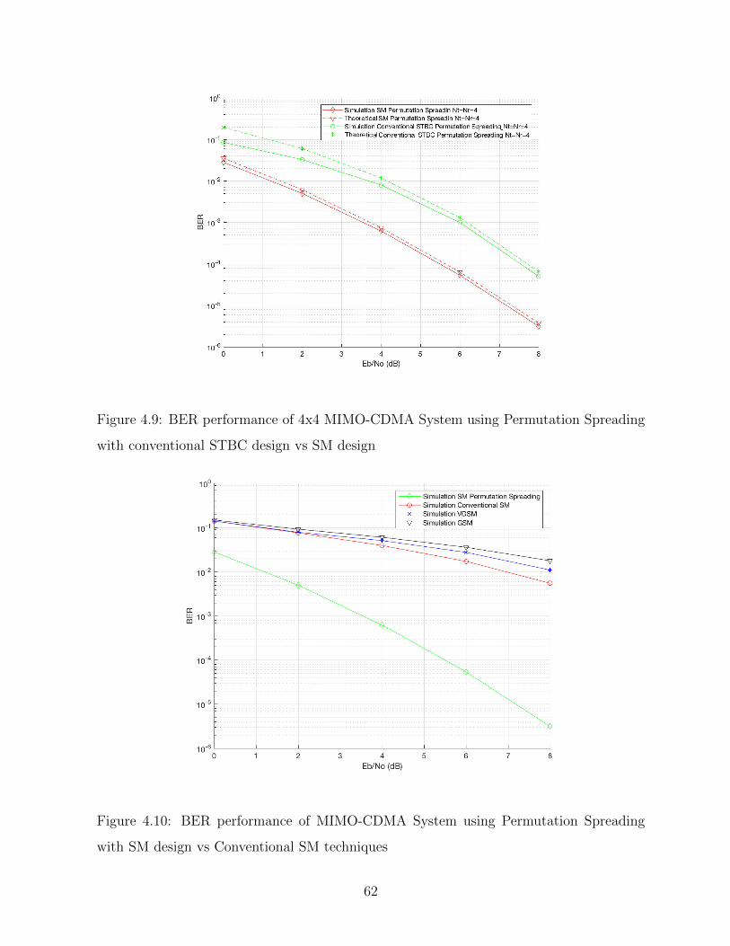
Figure 4.9: BER performance of 4x4 MIMO-CDMA System using Permutation Spreading
with conventional STBC design vs SM design
Figure 4.10: BER performance of MIMO-CDMA System using Permutation Spreading
with SM design vs Conventional SM techniques
62

4.4.3 Discussion
In this chapter, a novel technique for MIMO-CDMA system with permutation spread-
ing using SM is introduced. It is shown how the spatial positions of transmit antennas
can be combined with permutation spreading technique in order to create an additional
dependency between the data bits and the antennas combinations. This leads to an en-
hance of the system performance of MIMO systems. An analytical expression of the BER
was derived for the proposed technique under a frequency non-selective Rayleigh fading
channel with independent gains and perfect knowledge of the channel state information
(CSI) at the receiver. The obtained results were compared to the conventional permuta-
tion spreading technique using STBC design. Results show that the proposed technique
provides significant improvement of the BER performance of about 2dB for an SNR less
than 10dB in the case of a 4x4 MIMO system compared to STBC design. Moreover, a
comparison between the analytical expression and the simulated performance was shown.
The comparison shows that the theoretical expression is close to the simulation results and
it is tight as the SNR increases. Finally, a comparison between the proposed technique
and the conventional STBC and SM design was presented. Simulation results show that
the new SM designs outperform the performance of the conventional techniques.
63

Chapter 5
Multiuser Permutation Spreading
Employing Spatial Modulation For
Synchronous MIMO-CDMA systems
5.1 Introduction
In the MIMO-CDMA systems that were discussed in the previous chapter, only the single
user scenarios were treated for the proposed permutation spreading technique. In this
chapter, the focus shifts to multiple user scenario in synchronous transmission. In such a
model, each user generates exactly one message vector during the signalling interval and all
users signals are received by the receiver with no relative delay. Therefore, at the receiver,
all users’ messages begin and end at the same time. This is unlike the asynchronous case,
where the interference caused to one user’s message has contributions from two of each of
the other users’ messages [29]. This multiple access interference (MAI) hugely affects the
BER performance of all users who transmit simultaneously on the channel, and thus, an
investigation of the effect of MAI on BER of our proposed system is needed..
In CDMA systems, all users share the same spectrum by using a set of mutually or-
thogonal spreading sequences that are unique for each user [40]. However, this requires
increasing the length of the spreading sequences (chip rate) and thus reducing the spectral
64
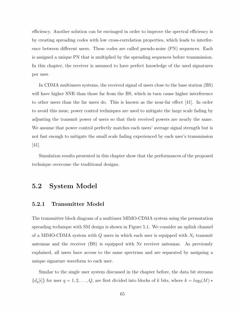
efficiency. Another solution can be envisaged in order to improve the spectral efficiency is
by creating spreading codes with low cross-correlation properties, which leads to interfer-
ence between different users. These codes are called pseudo-noise (PN) sequences. Each
is assigned a unique PN that is multiplied by the spreading sequences before transmission.
In this chapter, the receiver is assumed to have perfect knowledge of the used signatures
per user.
In CDMA multiusers systems, the received signal of users close to the base station (BS)
will have higher SNR than those far from the BS, which in turn cause higher interference
to other users than the far users do. This is known as the near-far effect [41]. In order
to avoid this issue, power control techniques are used to mitigate the large scale fading by
adjusting the transmit power of users so that their received powers are nearly the same.
We assume that power control perfectly matches each users’ average signal strength but is
not fast enough to mitigate the small scale fading experienced by each user’s transmission
[41].
Simulation results presented in this chapter show that the performances of the proposed
technique overcome the traditional designs.
5.2 System Model
5.2.1 Transmitter Model
The transmitter block diagram of a multiuser MIMO-CDMA system using the permutation
spreading technique with SM design is shown in Figure 5.1. We consider an uplink channel
of a MIMO-CDMA system with Q users in which each user is equipped with Nt transmit
antennas and the receiver (BS) is equipped with Nr receiver antennas. As previously
explained, all users have access to the same spectrum and are separated by assigning a
unique signature waveform to each user.
Similar to the single user system discussed in the chapter before, the data bit streams
{dq[i]} for user q = 1, 2, . . . , Q, are first divided into blocks of k bits, where k = log2(M) ∗
65
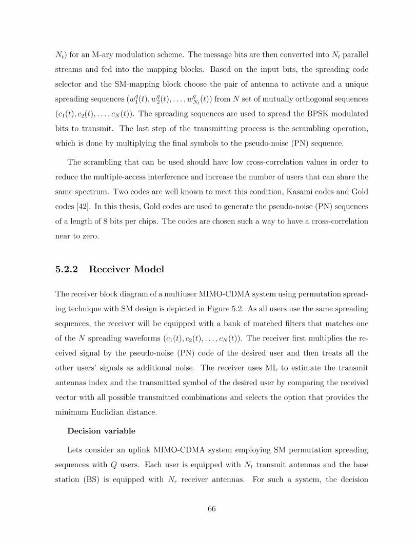
Nt) for an M-ary modulation scheme. The message bits are then converted into Nt parallel
streams and fed into the mapping blocks. Based on the input bits, the spreading code
selector and the SM-mapping block choose the pair of antenna to activate and a unique
spreading sequences (wq1(t), w
q2(t), . . . , w
qNt
(t)) from N set of mutually orthogonal sequences
(c1(t), c2(t), . . . , cN(t)). The spreading sequences are used to spread the BPSK modulated
bits to transmit. The last step of the transmitting process is the scrambling operation,
which is done by multiplying the final symbols to the pseudo-noise (PN) sequence.
The scrambling that can be used should have low cross-correlation values in order to
reduce the multiple-access interference and increase the number of users that can share the
same spectrum. Two codes are well known to meet this condition, Kasami codes and Gold
codes [42]. In this thesis, Gold codes are used to generate the pseudo-noise (PN) sequences
of a length of 8 bits per chips. The codes are chosen such a way to have a cross-correlation
near to zero.
5.2.2 Receiver Model
The receiver block diagram of a multiuser MIMO-CDMA system using permutation spread-
ing technique with SM design is depicted in Figure 5.2. As all users use the same spreading
sequences, the receiver will be equipped with a bank of matched filters that matches one
of the N spreading waveforms (c1(t), c2(t), . . . , cN(t)). The receiver first multiplies the re-
ceived signal by the pseudo-noise (PN) code of the desired user and then treats all the
other users’ signals as additional noise. The receiver uses ML to estimate the transmit
antennas index and the transmitted symbol of the desired user by comparing the received
vector with all possible transmitted combinations and selects the option that provides the
minimum Euclidian distance.
Decision variable
Lets consider an uplink MIMO-CDMA system employing SM permutation spreading
sequences with Q users. Each user is equipped with Nt transmit antennas and the base
station (BS) is equipped with Nr receiver antennas. For such a system, the decision
66

Figure 5.1: Multiuser transmitter of MIMO-CDMA with permutation spreading using SM
67
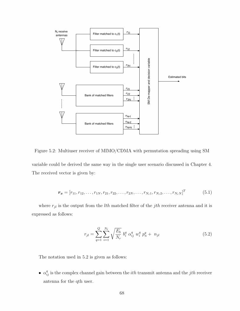
Figure 5.2: Multiuser receiver of MIMO/CDMA with permutation spreading using SM
variable could be derived the same way in the single user scenario discussed in Chapter 4.
The received vector is given by:
rx = [r11, r12, . . . , r1N , r21, r22, . . . , r2N , . . . , rNr1, rNr2, . . . , rNrN ]T (5.1)
where rjl is the output from the lth matched filter of the jth receiver antenna and it is
expressed as follows:
rjl =
Q∑q=1
Nt∑i=1
√Eb
Nr
bqi αqij w
qi p
qn + njl (5.2)
The notation used in 5.2 is given as follows:
• αqij is the complex channel gain between the ith transmit antenna and the jth receiver
antenna for the qth user.
68

• njl is the sampled noise after the lth matched filter of the jth receiver antenna.
• bqi is bit symbol transmitted by the qth user using antenna i.
• pqn is the pseudo-noise code generated for the qth user.
For a given user q, the receiver treats the other users’ signals as noise and uses ML
to estimate the transmitted data of the qth user. In fact, if we consider that the desired
signal to process is from user 1, the received signal could be rewritten as follows:
rx = u1b + n′ (5.3)
where:
• n′ is the noise matrix and it’s given by: n′ = [n′11, . . . , n′1N , n
′21, . . . , n
′2N , n
′Nr1
, . . . , n′NrN ]
where n′jl =Q∑
q=2
Nt∑i=1
√Eb
Nrbqi α
qij w
qi (t) p
qn + njl
• ub =Nt∑i=1
√Eb
Nrb1i α
1ij w
1i (t) p
1n is the received data matrix from the 1st receiver.
The decision variable, of the qth user, for a multiuser MIMO-CDMA system with
permutation spreading sequences using spatial modulation is given by:
(p, b) =M
minj=1
∥∥∥rx − uqb
∥∥∥2 (5.4)
where uqb is the vector made up of all possible received vector, of the desired user q
with the absence of the noise.
5.3 Simulation results and discussion
5.3.1 Simulation results comparison
The simulation results of the BER performance are shown in this section. We consider
a synchronous MIMO-CDMA system with 4 transmit antennas and 4 receiver antennas.
69

The simulations are performed under the same assumptions as chapter 4 where all channel
gains are considered to be independent, frequency non-selective and perfect channel state
information (CSI) is considered to be available at the receiver with zero power penalties.
We assume that all users are assigned with the same orthogonal spreading codes. These
sequences are generated using Hadamard codes with length of 8 bits per chip sequence.
The selection of the spreading sequences and the transmit antennas to activate are based
on Table 4.3. Pseudo-noise (PN) sequences are used to separate each user and they are
generated using Gold codes with a length of 8 bits per chip. The codes are chosen such
a way to minimize the cross-correlation value [43]. Finally, we assume that all users have
the same averaging SNR.
The BER performance of the multiuser MIMO-CDMA system employing permutation
spreading sequences with SM design for 2, 3 and 4 users scenario are shown in Figure 5.3.
A comparison between all these scenarios and the STBC permutation spreading sequences
for a multiuser MIMO-CDMA system with 4 transmit antennas and 4 receiver antennas is
shown in Figure 5.4.
From these figures, it can be seen that the BER performance decreases as more as we
add users to the system. Moreover, we can observe that at high SNR values an error floor
for a system with 3 users start to appear for a BER around 3 ∗ 10−5 and around 10−4 for
4 users system. In the single user system discussed in chapter 4, only a pair of transmit
antenna is activated at each signalling interval, which decreases the ICI and therefore en-
hance the system performance. However, in the multiuser system more transmit antennas
are involved which increase the ICI effect and reduce the BER performance as it can be
observed from the simulation results.
In order to keep the same spectral efficiency, all users use the same orthogonal spreading
sequences and scrambling codes are used to separate users from each other. However, these
codes are not perfectly orthogonal and their cross-correlations are not always near to zero.
Thus, for high SNR we can observe that more we increase the number of users more the
probability of having sequences with high cross-correlation values increases. This effect
leads to situations where codes sequences with low minimum distance are used, which
70

results the error floor.
The comparison between the SM design and the STBC design presented in Figure 5.4.
shows that the new design outperform the conventional method. It can be seen that the
4 users system with SM design provides better performance than the single user system
with STBC design for a BER greater than 6 ∗ 10−4.
Figure 5.3: Comparison of BER Performance of 4x4 MISO-CDMA System using SM Per-
mutation Spreading design
5.3.2 Discussion
In this chapter, the multiusers scenario for the proposed MIMO-CDMA system with per-
mutation spreading sequences using SM is discussed. In such a system, all users are
considered to share the same spreading sequences and use scrambling codes to separate
user’s information from each other. The receiver estimates the desired user information by
considering the other users’ signal as additional noise. The simulation results show that
the new design still outperforms the STBC design in synchronous multiuser transmission.
However, for high SNR values the SM design has higher error floor compared to the STBC
71
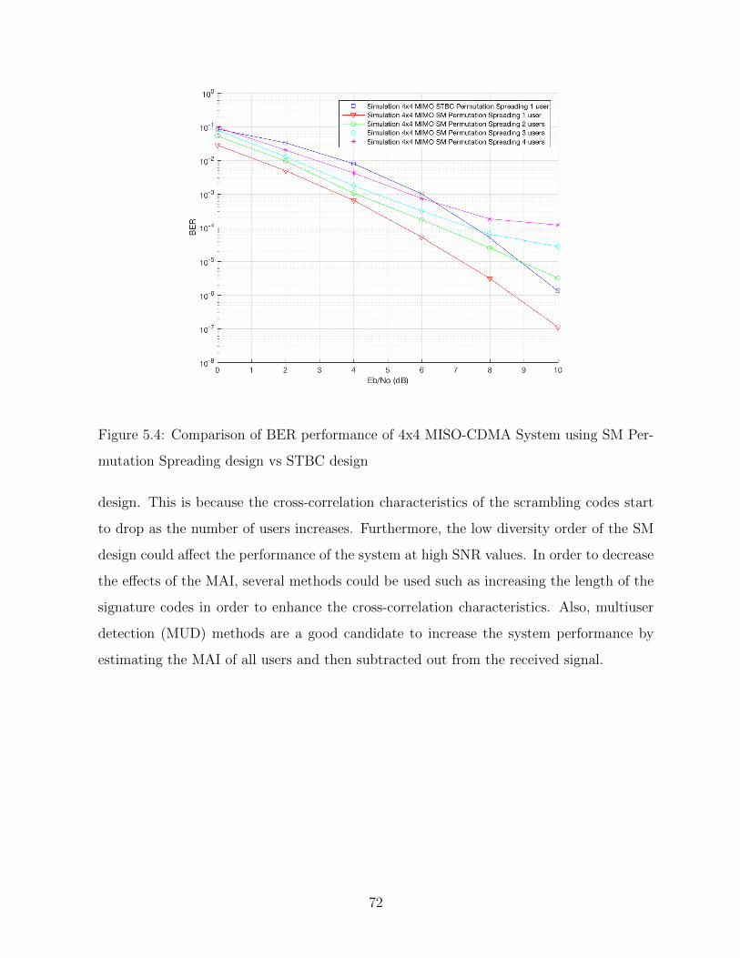
Figure 5.4: Comparison of BER performance of 4x4 MISO-CDMA System using SM Per-
mutation Spreading design vs STBC design
design. This is because the cross-correlation characteristics of the scrambling codes start
to drop as the number of users increases. Furthermore, the low diversity order of the SM
design could affect the performance of the system at high SNR values. In order to decrease
the effects of the MAI, several methods could be used such as increasing the length of the
signature codes in order to enhance the cross-correlation characteristics. Also, multiuser
detection (MUD) methods are a good candidate to increase the system performance by
estimating the MAI of all users and then subtracted out from the received signal.
72
Chapter 6
Conclusion and suggestion for future
work
6.1 Conclusion
In this thesis, we have proposed a new modulation technique for MIMO-CDMA systems
that takes the advantage of both SM-design and permutation spreading design. This study
discussed the benefits of combining the conventional permutation spreading techniques for
MIMO-CDMA with the new SM design and how could this strategy increase the system
performance in terms of spectral and power efficiency for single and multiuser scenarios.
In chapter 2, the concept of the parity bit selected sequences and permutation spreading
sequences for MIMO-CDMA systems was presented. The chapter discussed the difference
between the existing design strategies for the permutation spreading technique, such as
T-design and STBC design, and the parity bit selected spreading technique. Simulation
results showed that the permutation spreading methods provide better BER performance
compared to parity bit selected spreading technique. Moreover, results indicated that
the permutation spreading using STBC design provides slightly improvement in the BER
performance comparing to T-design without any increase of the system complexity.
Chapter 3 presented an overview of the SM methods. It explained how the position of
73

the transmit antennas could be used in order to increase the data rate and decrease the
number of RF-chains. The chapter also discussed the generalized idea of Spatial Modula-
tion (GSM) in which more than one transmit antennas can be activated to send same data
at each signaling interval. Furthermore, this chapter introduced an extension method of
GSM where the number of transmit antennas to activate, at each signaling interval, varies
from one transmit antenna to more than one. Simulation results showed that the perfor-
mance of these three techniques is close to each other with slightly better BER performance
of SM.
Chapter 4 introduced the proposed MIMO-CDMA system with permutation spreading
using SM. It showed how the spatial positions of transmit antennas can be combined with
permutation spreading technique in order to create an additional dependency between the
data bits and the antennas combinations and thus increase the spectral efficiency of the
system. The analytical expression of the BER was derived using the union bound method.
Simulation and theoretical results showed that that the proposed technique provides sig-
nificant improvement of the BER performance compared to the conventional STBC design
and the conventional SM.
In chapter 5, the multiusers scenario of the proposed technique was discussed. Inspired
from the NOMA technique, all users were considered to use the same spreading sequences
and scrambling codes that are quasi-orthogonal, were used to separate the users’ signals at
the receiver. Verified by simulation results, the proposed technique showed better perfor-
mance compared to conventional methods. However, for high SNR values the new design
had higher error floor.
6.2 Potential future work
The following are some suggestions for future work of this thesis:
• Investigate the BER performance of the multiuser scenario when MUD methods,
such as successive interferences cancelation (SIC), are used.
74
• Evaluate the performance of the proposed method under different frequency selective
fading channels
• Evaluate the performance of the proposed technique in partial CSI instead of perfect
CSI.
• The application of the proposed concept in OFDM systems. Similar to the SM-
MIMO-CDMA technique, the SM idea can be applied and parity bits can be used to
select the sub-carries used to transmit the signal.
75

References
[1] Ericsson. More than 50 billion connected devices. White Paper, February 2011.
[2] Andreas Molisch. Wireless communications. Wiley IEEE, Chichester, West Sussex,
U.K, 2011.
[3] 3GPP TR36.913, V10.0.0. 3GPP specification: Requirements for further advancements
for E-UTRA (LTE Advanced) (Release 10), Apr. 2011.
[4] Stefania Sesia. LTE - the UMTS long term evolution : from theory to practice. Wiley,
Chichester, 2011.
[5] Cheng-Xiang Wang, Fourat Haider, Xiqi Gao, Xiaohu You, Yang Yang, Dongfeng
Yuan, Hadi M. Aggoune, Harald Haas, S. Fletcher, and Erol Hepsaydir. Cellular
architecture and key technologies for 5g wireless communication networks. IEEE
Communications Magazine, 52(2):122–130, 2014.
[6] Jeffrey G. Andrews, Stefano Buzzi, Wan Choi, Stephen V. Hanly, Angel E. Lozano,
Anthony C. K. Soong, and Jianzhong (Charlie) Zhang. What will 5g be? CoRR,
abs/1405.2957, 2014.
[7] S. Wu, H. Wang, and C. H. Youn. Visible light communications for 5g wireless
networking systems: from fixed to mobile communications. IEEE Network, 28(6):41–
45, Nov 2014.
[8] F. Boccardi, R. W. Heath, A. Lozano, T. L. Marzetta, and P. Popovski. Five disruptive
technology directions for 5g. IEEE Communications Magazine, 52(2):74–80, February
2014.
76
[9] M. Di Renzo, H. Haas, A. Ghrayeb, S. Sugiura, and L. Hanzo. Spatial modulation for
generalized mimo: Challenges, opportunities, and implementation. Proceedings of the
IEEE, 102(1):56–103, Jan 2014.
[10] M. D. Renzo, H. Haas, and P. M. Grant. Spatial modulation for multiple-antenna wire-
less systems: a survey. IEEE Communications Magazine, 49(12):182–191, December
2011.
[11] A. Stavridis, S. Sinanovic, M. Di Renzo, H. Haas, and P. Grant. An energy saving
base station employing spatial modulation. In 2012 IEEE 17th International Work-
shop on Computer Aided Modeling and Design of Communication Links and Networks
(CAMAD), pages 231–235, Sept 2012.
[12] M. Di Renzo and H. Haas. On transmit diversity for spatial modulation mimo: Im-
pact of spatial constellation diagram and shaping filters at the transmitter. IEEE
Transactions on Vehicular Technology, 62(6):2507–2531, July 2013.
[13] M. Taherzadeh, H. Nikopour, A. Bayesteh, and H. Baligh. Scma codebook design. In
2014 IEEE 80th Vehicular Technology Conference (VTC2014-Fall), pages 1–5, Sept
2014.
[14] M. AL-Imari, M. A. Imran, R. Tafazolli, and D. Chen. Performance evaluation of low
density spreading multiple access. In 2012 8th International Wireless Communications
and Mobile Computing Conference (IWCMC), pages 383–388, Aug 2012.
[15] Shanzhi Chen, Bin Ren, Qiubin Gao, Shaoli Kang, Shaohui Sun, and Kai Niu. Pattern
division multiple access - a novel nonorthogonal multiple access for fifth-generation
radio networks. IEEE Trans. Vehicular Technology, 66(4):3185–3196, 2017.
[16] D. Fang, Y. C. Huang, Z. Ding, G. Geraci, S. L. Shieh, and H. Claussen. Lattice
partition multiple access: A new method of downlink non-orthogonal multiuser trans-
missions. In 2016 IEEE Global Communications Conference (GLOBECOM), pages
1–6, Dec 2016.
77
[17] Z. Ding, Y. Liu, J. Choi, Q. Sun, M. Elkashlan, C. L. I, and H. V. Poor. Application
of non-orthogonal multiple access in lte and 5g networks. IEEE Communications
Magazine, 55(2):185–191, February 2017.
[18] 3rd Generation Partnership Project (3GPP). Study on downlink multiuser superposi-
tion transmission for LTE, Mar. 2015.
[19] Ping Yang, Yue Xiao, Bin Zhou, and Shaoqian Li. Initial performance evaluation of
spatial modulation ofdm in lte-based systems. In CHINACOM, pages 102–107. IEEE
Computer Society, 2011.
[20] D. Sinanovic, G. Sisul, and B. Modlic. Low-papr spatial modulation for sc-fdma. IEEE
Transactions on Vehicular Technology, 66(1):443–454, Jan 2017.
[21] M. Fukuma and K. Ishii. Space-time code division multiple access based on spatial
modulation. In 2015 IEEE 82nd Vehicular Technology Conference (VTC2015-Fall),
pages 1–5, Sept 2015.
[22] C. D’Amours and J. Y. Chouinard. Parity bit selected and permutation spreading
for cdma/mimo systems in frequency-nonselective rayleigh fading channels. In 2007
IEEE 65th Vehicular Technology Conference - VTC2007-Spring, pages 1475–1479,
April 2007.
[23] BG Gopal and PG Kuppusamy. A comparative study on 4g and 5g technology for
wireless applications. Journal of Electronics and Communication Engineering (IOSR-
JECE), 10(6):67–72, 2015.
[24] C. D’Amours. Parity bit selected spreading sequences: a block coding approach to
spread spectrum. IEEE Communications Letters, 9(1):16–18, Jan 2005.
[25] M. Shi, C. D’Amours, and A. Yongacoglu. Design of spreading permutations for mimo-
cdma based on space-time block codes. IEEE Communications Letters, 14(1):36–38,
January 2010.
78

[26] F.J. MacWilliams and N.J.A. Sloane. The Theory of Error-Correcting Codes. North-
holland Publishing Company, 2nd edition, 1978.
[27] V. Tarokh, H. Jafarkhani, and A. R. Calderbank. Space-time block codes from or-
thogonal designs. IEEE Transactions on Information Theory, 45(5):1456–1467, Jul
1999.
[28] C. D’Amours and J. Y. Chouinard. Parity bit selected and permutation spreading
for cdma/mimo systems in frequency-nonselective rayleigh fading channels. In 2007
IEEE 65th Vehicular Technology Conference - VTC2007-Spring, pages 1475–1479,
April 2007.
[29] Proakis. Digital Communications 5th Edition. McGraw Hill, 2007.
[30] Raed Yousef Mesleh. Spatial modulation: a spatial multiplexing technique for efficient
wireless data transmission. PhD thesis, Jacobs Uni Bremen, 2007.
[31] R. Mesleh, M. D. Renzo, H. Haas, and P. M. Grant. Trellis coded spatial modulation.
IEEE Transactions on Wireless Communications, 9(7):2349–2361, July 2010.
[32] N. Serafimovski, A. Younis, R. Mesleh, P. Chambers, M. Di Renzo, C. X. Wang, P. M.
Grant, M. A. Beach, and H. Haas. Practical implementation of spatial modulation.
IEEE Transactions on Vehicular Technology, 62(9):4511–4523, Nov 2013.
[33] A. Younis, N. Serafimovski, R. Mesleh, and H. Haas. Generalised spatial modula-
tion. In 2010 Conference Record of the Forty Fourth Asilomar Conference on Signals,
Systems and Computers, pages 1498–1502, Nov 2010.
[34] J. Jeganathan, A. Ghrayeb, and L. Szczecinski. Generalized space shift keying modu-
lation for mimo channels. In 2008 IEEE 19th International Symposium on Personal,
Indoor and Mobile Radio Communications, pages 1–5, Sept 2008.
[35] N. Serafimovski, M. D. Renzo, S. Sinanovic, R. Y. Mesleh, and H. Haas. Fractional bit
encoded spatial modulation (fbe-sm). IEEE Communications Letters, 14(5):429–431,
May 2010.
79

[36] A. Younis, R. Mesleh, H. Haas, and P. M. Grant. Reduced complexity sphere decoder
for spatial modulation detection receivers. In 2010 IEEE Global Telecommunications
Conference GLOBECOM 2010, pages 1–5, Dec 2010.
[37] J. Jeganathan, A. Ghrayeb, and L. Szczecinski. Spatial modulation: optimal detection
and performance analysis. IEEE Communications Letters, 12(8):545–547, Aug 2008.
[38] Emanuele Viterbo and Joseph Boutros. A universal lattice code decoder for fading
channels. IEEE Trans. Information Theory, 45(5):1639–1642, 1999.
[39] Abdelhamid Younis. Spatial modulation: theory to practice. Ph.D. dissertation, 2014.
[40] Sergio Verdu. Multiuser detection. Cambridge University Press, CambridgeK New
York, 1998.
[41] Abdurazak Mudesir. Power control algorithm in cdma systems. International Univer-
sity Bremen, 11, 2004.
[42] S. Sriram and V. Sundararajan. Efficient pseudo-noise sequence generation for spread-
spectrum applications. In IEEE Workshop on Signal Processing Systems, pages 80–86,
Oct 2002.
[43] H. Vincent Poor and Sergio Verdu. Single-user detectors for multiuser channels. IEEE
Trans. Communications, 36(1):50–60, 1988.
80