Persistent collective trend in stock markets

Emeric BaloghDepartment of Theoretical Physics, Babeş-Bolyai University, RO-400084 Cluj-Napoca, Romania and Department of Optics

and Quantum Electronics, University of Szeged, HU-6720 Szeged, Hungary

Ingve Simonsen*Department of Physics, Norwegian University of Science and Technology (NTNU), NO-7491 Trondheim, Norway

Bálint Zs. NagyFaculty of Economics and Business Administration, Babeş-Bolyai University, RO-400591 Cluj-Napoca, Romania

Zoltán NédaDepartment of Theoretical Physics, Babeş-Bolyai University, RO-400084 Cluj-Napoca, Romania

�Received 3 June 2010; revised manuscript received 20 October 2010; published 13 December 2010�

Empirical evidence is given for a significant difference in the collective trend of the share prices during thestock index rising and falling periods. Data on the Dow Jones Industrial Average and its stock components arestudied between 1991 and 2008. Pearson-type correlations are computed between the stocks and averaged overstock pairs and time. The results indicate a general trend: whenever the stock index is falling the stock pricesare changing in a more correlated manner than in case the stock index is ascending. A thorough statisticalanalysis of the data shows that the observed difference is significant, suggesting a constant fear factor amongstockholders.

DOI: 10.1103/PhysRevE.82.066113 PACS number�s�: 89.65.Gh

I. INTRODUCTION

The world is once again experiencing a major financial-economic crisis, the worst since the crash of October 1929that initiated the great depression of the 1930s. Many citi-zens are concerned for obvious reasons; we are facing globalrecession; banks and financial institutions go bankrupt; com-panies struggle to get credit and many are forced to reducetheir workforce or even go out of business. Interest rates areincreasing while private savings invested in the stock marketevaporate. Large parts of our contemporary societies aredeeply affected by the new financial reality.

The current financial crisis is one particular dramatic ex-ample of collective effects in stock markets �1–4�; duringcrises nearly all stocks drop in value simultaneously. Fortu-nately, such extreme situations are relatively rare. What isless known, however, is that during more normal “noncriti-cal” periods, collective effects do still represent characteris-tics of stock markets that in particular influence their shorttime behavior. One such effect will be addressed in this pub-lication, where our aim is to present empirical evidence foran asymmetry in stock-stock correlations conditioned by thesize and direction of market moves. In particular, we willpresent empirical results showing that when the Dow JonesIndustrial Average �DJIA� index �“the market”� is dropping,then there exists a significantly stronger stock-stock correla-tion than during times of a rising market. Our results indicatethat such enhanced �conditional� stock-stock correlations arenot only relevant during times of dramatic market crashes,but instead represents features of markets during more “nor-mal” periods.

There is certainly the aspect of market microstructurewhenever we examine the collective behavior of stock mar-ket participants. Ever since the stock market crash of 1987,programmed trading has many times been cited as a possiblefactor behind the acceleration of downward movements dur-ing a market crash. Certainly the advancement of these algo-rithmic trading platforms contributes to increasing correla-tion between stock movements but we believe that thesealgorithms produce symmetric correlations and cannot ac-count for the asymmetry documented in the present paper.

II. INVERSE STATISTICS

Distribution of returns is traditionally used as one of theproxies for the performance of stocks and markets over acertain time history �1–3�. In the economics, finance, andeconometrics literature the problem of market sentiment andinvestor confidence is usually addressed by the use of vari-ous indicators. These indicators are either derived from ob-jective market data �5�, or obtained by conductingquestionnaire-based surveys among professional and indi-vidual investors �6�. In the present study we consider thus thefirst approach, since we believe that the market data �pricesand returns� are more objective proxies than questionnaire-inferred data.

The basic quantity of interest is the logarithmic return,defined as the �natural� logarithm of the relative price changeover a fixed time interval �t, i.e.,

r�t�t� = ln� p�t + �t�p�t�

� , �1�

where p�t� denotes the asset price at time t �1–3�. In additionto this basic quantity, it is also desirable to have available a*ingve.simonsen@phys.ntnu.no; http://web.phys.ntnu.no/~ingves

PHYSICAL REVIEW E 82, 066113 �2010�

1539-3755/2010/82�6�/066113�9� ©2010 The American Physical Society066113-1

time-dependent proxy where the asset performance is gaugedover a nonconstant time interval. One such approach is theso-called inverse statistics approach �7–10� recently intro-duced and adapted to finance from the study of turbulence�11,12�. The main idea underlying this method is to not fixthe time interval �or window�, �t in Eq. �1�, but instead toturn the question around and ask for what is the �shortest�waiting time, ��, needed to reach a given �fixed� return level,�, for the first time when the initial investment was made attime t �see Ref. �7� for details�,

� � r���t� . �2�

Hence, the inverse statistics approach concerns itself with thestudy of the distribution of waiting times �13� that in thefollowing will be denoted by p����.

Recently, this method of analysis has been applied to thestudy of various single stocks and market indices, both frommature and emerging markets, as well as to foreign exchangedata and even artificial markets �7–10,14–21�. The waitingtime histograms possess well-defined and pronounced��-dependent� maxima �7� �Fig. 1�a�� followed by tails thathave been claimed to have a power-law decay p�������

−�

�7–10,13�. Although it is not the purpose of the present paperto prove or disprove this statement, our results suggest anexponent ��3 /2 �Fig. 1�b��, a value that is a consequenceof the uncorrelated increments of the underlying asset priceprocess �13�. However, to rigorously prove the power-law

assumption, a detailed analysis would be necessary, and itcan be done, for instance, by following the method proposedin Ref. �22�.

Studies of single stocks, for given �moderate� positive andnegative levels of returns, ��, have revealed, almost sym-metric waiting time distributions �Fig. 2� �15,21,23�. Unex-pectedly, however, stock index data seem not to share thisfeature. They do instead give raise to asymmetric waitingtime distributions �Fig. 1�a�� for return levels � for whichthe corresponding single stock distributions were symmetric�15,23�. This asymmetry is expressed by negative return lev-els being reached sooner than those corresponding to posi-tive levels �of the same magnitude of ��. This effect wastermed the gain-loss asymmetry �7� and has later been ob-served for many major stock indices �7,8,18,19,24,25�. It ishere important to note that the gain-loss asymmetry is not aconsequence of the generally long-term positive trend �ordrift� of the data since this was removed by considering anaverage with a suitable window size on the prices. The long-term positive trend will affect long waiting times and wouldinduce shorter waiting times for the positive return levels.However, empirically one finds that the waiting times of in-dices are shortest for negative return levels—the opposite ofwhat is to be expected from the long term trend effect. Inpassing we note that recently it has been found that alsosingle stocks may show some degree of gain-loss asymmetrywhen the level of return, �, is getting sufficiently large�21,26�. However, it still remains true that for not too largereturn levels, e.g., �=0.05, the waiting time distributions for

FIG. 1. �Color online� Inverse statistics results for logarithmic return levels of �= �5% for the DJIA index �data between 1991 and2008�. The figures show the gain-loss asymmetry; open green triangles represents ��0, while filled red circles refer to ��0. On thelog-linear scale �a� the asymmetry is more evident, while on log-log scale �b� the power-law nature of the tail of the distribution isobservable. The dashed line indicates the slope −3 /2.

FIG. 2. �Color online� Same asFig. 1, but now for the DJIAstocks: �a� General Motors and �b�McDonald’s Corp. Notice thatgain-loss asymmetry is not ob-served in this case.

BALOGH et al. PHYSICAL REVIEW E 82, 066113 �2010�

066113-2

single stocks are symmetric to a good approximation �21�.The presence of a gain-loss asymmetry in an index may

seem like a paradox since the value of a stock index is es-sentially the �weighted� average of the individual constitut-ing stocks. Even so, one does observe an asymmetric waitingtime distribution for the index comprised of �more-or-less�symmetric single stocks. How can this be rationalized? Re-cently, a minimal �toy� model—termed the fear factormodel—was constructed for the purpose of explaining thisapparent paradox �23�. The key ingredient of this model isthe so-called collective fear factor, a concept similar to syn-chronization �27�. At certain times, controlled by a “fear fac-tor,” the stocks of the model all move downward, while atother times they move independently of each other. This isdone in a way that the price processes of the single stocks are�over a long time period� guaranteed to produce symmetricwaiting time distributions �and uncorrelated price incre-ments�. The fear-factor model, that qualitatively reproduceswell empirical findings, introduces collective downwardmovements among the constituting stocks. The model syn-chronizes downward stock moves, or in other words, it hasstronger stock-stock correlations during dropping marketsthan during market raises. This means that the fear factor ofthe stockholders is stronger than their optimism factor onaverage. This is consistent with the findings of Kahnemanand Tversky �28�, reported in the economics literature, thatdemonstrate that the utility loss of negative returns is largerthan the utility gain for positive returns in the case of mostinvestors.

Recently, the idea of the fear-factor model �23� was re-considered and generalized by Siven et al. �25� by allowingfor longer time periods of stock comovement �correlations�.These authors also find that the gain-loss asymmetry is along time scale phenomena �25�, and that it is related tosome correlation properties present in the time series �21�. Itwas also proposed that the gain-loss asymmetry is in closerelationship with the asymmetric volatility models �exponen-tial generalised autoregressive conditional heteroskedastic-ity� used by econometricians �29�.

Furthermore, also additional explanations for the gain-loss asymmetry have been proposed in the literature. Thoseinclude the leverage effect �2,30–32�, and regime switchingmodels �26�. Bouchaud et al. �30� emphasize different be-haviors at the level of individual stocks and at the marketindex level �the weak and strong leverage effect�, differenceattributed to a certain “panic effect.” This model uses a re-tarded volatility specification, which breaks down at the in-dex level, because according to the authors, “a specific riskaversion phenomenon seems to be responsible for the en-hanced observed negative correlation between volatility andreturns.” Ciliberti et al. �33� further developed this model by

examining the implications of volatility leverage for optiontrading strategies and also identifying a relationship betweenthe magnitude of the leverage effect and the size �marketcapitalization� of stocks. So far, it is fair to say that the originof the gain-loss asymmetry is still �partly� debated in theliterature. A recent article by Lisa Borland �34� demonstrates,among other things, the stronger stock cross-correlations intimes of “panic.” This paper examines the relationship be-tween the second �variance or volatility� and fourth moments�kurtosis� of the distribution of returns. An interesting findingis that there is an inverse relationship between volatility�variance� and kurtosis, a finding explained by the conjecturethat in times of panic, although volatility is higher than innormal times, it is more uniform, affecting simultaneously allstocks. However, the author uses a correlation measure,which we find less informative, since it uses only the numberof stocks rising and falling and not how much they change.We believe that in order to obtain a truly reliable correlationmeasure, one has to include effects of the magnitude of pricechanges, and this can be attained through statistical measuressuch as the Pearson correlation coefficient.

The key idea of the fear factor model �21,23� is the en-hanced stock-stock correlations during periods of fallingmarket. Up to now this idea has not been supported by em-pirical data. In this work, we conduct such a delicate statis-tical analysis, and we are able to show, based on empiricaldata, that indeed there exist a stronger stock-stock correla-tions during falling, as compared to rising, market.

III. CONDITIONAL MARKET COMPONENTCORRELATION FUNCTION

Let r�tx �t� denote the logarithmic return of stock x �from

the index under study� between time t and t+�t �the timeunit in the DJIA data is �t=1 trading day�. In order to fa-cilitate the coming discussion, we introduce the followingnotation for a mathematical average taken over a set A= A�t��t=t1

t2 :

�A�t� t=t1,t2= �A�t��t=t1

t2 =

�t=t1

t2

A�t�

A, �3�

where A denotes the cardinality of the set, i.e., the numberof elements in A. If no explicit limits are given for the av-erage �like in �A�t��t = �A�t� t�, all possible values will beassumed for t. In terms of this notation, a Pearson-type cor-relation can then be computed between each stock pair �x ,y�resulting in the following �equal time� stock-stock correla-tion function,

S�x,y��t,t,�t� =�r�t

x �t��r�ty �t�� t�=t,t+t − �r�t

x �t�� t�=t,t+t�r�ty �t�� t�=t,t+t

�tx �t;t��t

y �t;t�, �4�

PERSISTENT COLLECTIVE TREND IN STOCK MARKETS PHYSICAL REVIEW E 82, 066113 �2010�

066113-3

where �t� �t ;t� signifies the volatility of stock � ��=x ,y� at

time t �and time window t�, and is defined as

�t� �t;t� = ���r�t

� �t���2 t�=t,t+t − �r�t� �t�� t�=t,t+t

2 . �5�

Note that S�x,y��t ,t ,�t� contains two time scales; t is thetime window over which the average in Eq. �4� is calculated,while �t is the time interval used to define returns �cf. Eq.�1��.

By definition, the stock-stock correlation function,S�x,y��t ,t ,�t�, is specific to the asset pair �x ,y�, and doestherefore not represent the market as a whole. However, inorder to obtain a representative level of stock-stock correla-tion for the market �index�, we propose to averageS�x,y��t ,t ,�t� over all possible stock pairs �x ,y� contained inthe index. In this way, we are lead to introducing the marketcomponent correlation function,

S0�t,t,�t� = �S�x,y��t,t,�t� �x,y�. �6�

In passing, we note that the average contained in Eq. �6�potentially should be weighted so that the contribution to thecorrelation function S0�t ,t ,�t� from a stock pair �x ,y� isweighted with a factor that is proportional to the product ofthe weights associated with the two stocks and used to con-struct the value of the index. Typically this weight corre-sponds to the capitalization of the company in question.Since we here, however, are studying the DJIA—for whichall constituting stocks have the same weight in the index �anatypical situation�—this possibility has not been consideredhere and neither has the weight factor been included in thedefinition of S0�t ,t ,�t�.

The market component correlation function, as defined byEq. �6�, measures the overall level of stock-stock correlationsof the index �market� under investigation independent of ris-ing and falling market. However, what we have set out tostudy, is if there exists any significant difference betweenthese two latter cases. To this end, we introduce what webelow will refer to as the conditional market component cor-relation function, C0�� ,t ,�t�, that measures the typicalvalue of the market component correlations S0�t ,t ,�t�given that the �logarithmic� return of the index itself, rt�t� isabove �below� a given return threshold value �. Mathemati-cally, the conditional market component correlation functionis defined by the following conditional time average:

C0��,t,�t� = �C��,t,t,�t��t t, �7a�

where a time-dependent conditional market component cor-relation function set has been introduced as

C��,t,t,�t��t = �S0�t,t,�t�rt�t� � ��t if � � 0

S0�t,t,�t�rt�t� � ��t if � � 0� .

�7b�

A comparison of C0�+� ,t ,�t� and C0�−� ,t ,�t�,should in principle be able to reveal potential difference inthe level of stock-stock correlations during periods of risingand falling market conditions. If it is found that C0�� ,t ,�t�is symmetric with respect to the sign of �, the stock-stockcorrelations do not depend �very much� on the direction of

the market. On the other hand, if an asymmetry is observedin C0��� ,t ,�t� for a given �, this clearly indicates thatstock-stock correlations are dependent on market direction.Such results, being interesting in its own right, can practi-cally be used in risk and portfolio management. Moreover,they can be used as valuable input for developing more so-phisticated portfolio theories aiming at designing the optimalportfolio. The weights of securities in an optimal portfolio asmodeled by Markowitz �35� depend on the correlations andcovariance matrices between the returns of those securitiesand these correlations assume a uniform attitude toward risk.Our results suggest that these correlation matrices shouldtake into account the asymmetry in the correlations for thepositive and negative returns and, therefore, are consistentwith behavioral portfolio theory �36� that suggests differentattitudes toward risk in different domains for the same inves-tor.

Given the subtle nature of the correlations that we hereare trying to detect, we will introduce an additional timeaverage—now to be performed over the time scale t that allpreviously introduced correlation functions depend. The av-eraged conditional market component correlation function isdefined as

C��,�t� = �C0��,t,�t� t=t1,t2, �8�

where t1 and t2�t1 are time scales over which stock-stock correlations are relevant �given the type of data beinganalyzed�. The average over t in Eq. �8� is performed onlywith the purpose of improving the statistics. For stock indi-ces containing a large number of stocks �e.g., SP500 andNASDAQ�, this average may not be needed. However, forthe DJIA that currently contains only 30 stocks, this averageis of advantage.

The needed formalism is by now introduced, and we areready to use it for the empirical analysis. Here we are focus-ing on the DJIA, as mentioned previously, and the data to beanalyzed were obtained from Yahoo Finance �37�. The dataset consists of daily closing prices of the 30 DJIA stocks aswell as the DJIA index itself. It covers an 18 years periodfrom May 1991 to September 2008. Note that this periodincludes the development of the dot-com bubble in the late1990s and its subsequent burst in 2000, the 1997 minicrash�as a consequence of the Asian financial crisis of 1997�, thecollapse of the Long-Term Capital Management �as a conse-quence of the Russian financial crisis of 1998�, the early2000s recession as well as the worldwide economic-financialcrisis of 2007–2008.

With these data and the formalism presented previously,the averaged conditional market component correlation func-tion, C�� ,�t�, can be calculated. It is presented in Fig. 3 fora range of positive and negative return levels, ��, where ithas been assumed that �t=1 day, t1=10 day, and t2=35 day. Figure 3 shows a pronounced asymmetry betweenpositive and negative �index� return levels, ��. The stock-stock correlations, as given by C�� ,�t�, are systematicallystronger whenever the market is dropping ���0� than whenit is rising ���0�. This is found to be the case for the wholerange of considered levels of return �. It also worth notingthat in the limit �→0 there is a substantial difference be-

BALOGH et al. PHYSICAL REVIEW E 82, 066113 �2010�

066113-4

tween the conditional market component correlation for thepositive and negative returns: lim�→0+�C�−� ,�t�−C�� ,�t���0.07=7%. For the largest positive levelsshown, it is noted that the statistical quality of the data isseen to become poor.

Hence, the empirical results of Fig. 3 support the primaryassumption underlying the fear-factor model �23�; stocks areon average more strongly correlated �or synchronized�among themselves during falling than rising market condi-tions.

IV. STATISTICAL ANALYSIS OF THE RESULTS

The effect that we are studying here is rather subtle, andseveral averaging procedures had to be considered in order toidentify it. Hence, it is important to have confidence in theresults, and to make sure that they are not artifacts of theanalyzing method. Moreover, one also has to prove that the

obtained difference is a general feature of the stock marketand is not due to one �or a few� special events where, e.g.,the market crashes. To address these issues, additional analy-sis is required.

First, we revisited the averaging procedure over stockpairs used in defining Eq. �6�. The aim was to show that thedifference obtained in the measured correlations between thestocks for positive and negative levels of index returns wasindeed present for the majority of the stock pairs. For thispurpose, for each pair of stocks �x ,y� of the index, the aver-age C�x,y��� ,�t�= �C�x,y��� ,t ,�t� t=t1,t2

was considered,where the conditional stock-stock correlation function,C�x,y��� ,t ,�t�, is defined from S�x,y��t ,t ,�t� in a com-pletely analogous way to how C0�� ,t ,�t� was obtainedfrom S0�t ,t ,�t� in Eq. �7b�.

The distributions of the conditional stock-stock correla-tion function, C�x,y��� ,�t�, including all possible stock pairs�x�y� of the DJIA, is presented in Fig. 4 for some represen-tative levels of index return �=0.03, 0.05, and 0.10. Theresults of Fig. 4 indicate that the stock-stock correlations fora negative index return levels, −�, �plotted as red shadedareas� is for the majority of the stock pairs stronger than thestock-stock correlations for the corresponding positive level�plotted as green dashed areas�, and this observation appliesequally for all the index return levels considered. An alterna-tive way of illustrating this difference is to plot the distribu-tion of the relative difference ��= �C�x,y��−� ,�t�−C�x,y��� ,�t�� / C�x,y��� ,�t� �Fig. 5�. The clear asymmetryof this distribution with respective to ��=0 is an indicationthat the stock-stock correlations for a negative index returnlevel is in general stronger than the stock-stock correlationsfor the corresponding positive level �of the same magnitude�.

The indications obtained from Figs. 4 and 5 that the con-ditional stock-stock correlations are stronger for negativethan positive index return levels can also be confirmed morequantitatively by a statistical test. More precisely, we want tosee what is the chance that two random samples from thesame distribution would yield the observed difference in themean. A Wilcoxon-type nonparametric z-test �38� was per-formed and the results of the test are presented in Table I.The negative value of z suggests that the stock-stock corre-lations for the negative change in the index are indeed biggerthan those for the positive changes. The value of p is theprobability that finite samples from the same ensemble

FIG. 3. �Color online� The average conditional market compo-nent correlations, C�� ,�t�, between the stock components for vari-ous return rates, �, of the DJIA stock index. Open green trianglescorrespond the positive return levels ���0�, while filled red circlessignifies negative return levels ���0�. The stronger correlation incase of negative returns is readily observable from Fig. 3. In ob-taining these results, it was assumed that t1=10 day, t2

=35 day, and �t=1 day. For values of � larger than about 0.15,the statistics became poor. This was in particular the case for posi-tive values of �.

FIG. 4. �Color online� The distribution, p�C�x,y��, of the correlation function C�x,y��� ,�t� based on all possible stock pairs �x ,y� within theDJIA stock index �x�y�. Red shaded areas correspond to ��0, while the areas green dashed areas refer to ��0. The distributions are givenfor various values of the return level � as indicated in each panel ��t=1 day in all cases�.

PERSISTENT COLLECTIVE TREND IN STOCK MARKETS PHYSICAL REVIEW E 82, 066113 �2010�

066113-5

would yield the hypothesized differences in the mean. Theparameter p is thus a measure of the significance level,smaller values correspond to higher significance for the ob-tained differences in the mean. The results presented in TableI show that the difference in conditional stock-stock correla-tions is indeed significant.

Second, we wanted to make sure that the observed asym-metry in C0�� ,t ,�t�= �C�� , t ,t ,�t��t �Eq. �7�� was notcaused by a few isolated events—like large market drops—but instead represented a feature of the market that waspresent at �more-or-less� all times. For this purpose, we wentback and studied more carefully the time-dependent condi-tional market correlation function C�� , t ,t ,�t� �before thetime average�. More precisely, in order to improve the statis-tics, the following average was computed�C�� , t ,t ,�t� t=t1,t2

�Ct�� ,�t�. For fixed values of the in-dex return level �, and the time windows t1=10 days,t2=35 days, and �t=1 day, we compared the two distribu-tions p�Ct�+� ,�t�� and p�Ct�−� ,�t��. An asymmetry inC0�� ,t ,�t� being caused by a few isolated events inCt�� ,�t�, will produce almost identical distributions for thetwo cases �� that only differ by some infrequent “outliers”that are large enough to move the mean. On the other hand,a more systematic difference in Ct�� ,�t� for +� and−� will produce distinctly differences between thep�Ct�+� ,�t�� and p�Ct�−� ,�t�� distributions.

In Fig. 6 we present the empirical distributionsp�Ct�� ,�t�� of the DJIA for some typical positive and nega-

tive values of the index return level. These empirical resultspoint toward the two distributions p�Ct�+� ,�t�� andp�Ct�−� ,�t�� being different. To quantitatively show thatthey differ significantly, again a nonparametric Wilcoxon sig-nificance test was performed. However, in order to conductthis test it is necessary to have the same number of datapoints in the histograms for positive and negative index re-turn values. Since the Ct�� ,��-data did not had this propertywe had to ensure this condition. We first identified the setwith the smallest number of elements �usually this was theset corresponding the negative returns�, and then from theother set, the same number of elements were randomly se-lected. Here our assumption was that the random selectionwill not alter the normalized distribution. Results obtained bythis procedure for the same values of � used to produce Fig.6 are given in Table II. The extremely small values obtainedfor p suggest, as pointed out previously, that the differencebetween the two distributions, p�Ct�+� ,�t�� andp�Ct�−� ,�t��, is indeed significant also for this averagingstep.

Third, we address the level of conditional market correla-tion �C0�� ,t ,�t�� as a function of the size of the time win-dow t for �� �and �t=1 day� �Fig. 7�. Figure 7 showsthat systematically, and independent of t and � �at lest forthe values we have considered�, one finds that the condi-tional market correlations are higher for negative index re-turn levels �−�� than the corresponding positive levels�+��; i.e., C0�−� ,t ,�t��C0�+� ,t ,�t�. This suggeststhat the sign of the difference does not depend on the values

FIG. 5. �Color online� The distribution of the quantity ��= �C�x,y��−� ,�t�−C�x,y��� ,�t�� / C�x,y��� ,�t� obtained on the basis of theDJIA stock index for different return levels, �, as indicated in the figures. We recall that in the case of no asymmetry, the distribution, p����,should be symmetric around ��=0 �vertical dashed lines�.

FIG. 6. �Color online� The distribution of the correlations Ct�� ,�t���C�� , t ,t ,�t� t=t1,t2for different return levels, ��. Here the

green dashed areas correspond to ��0 while red shaded areas are used to indicate ��0. In obtaining these results it was assumed thatt1=10 day, t2=35 day, and �t=1 day.

BALOGH et al. PHYSICAL REVIEW E 82, 066113 �2010�

066113-6

considered for t1 and t2, used in performing the averageover t.

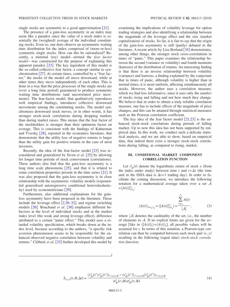
Finally, we investigate the time dependence of the differ-ence between the market component correlation functions�S0�t ,t ,�t�� for positive and negative return levels. Thiswill yield additional information on the observed asymmetryby visualizing the time periods that contribute with a signifi-cant difference to correlation calculations. For studying thiseffect for a fixed time window t we would, in principle,need a three-dimensional plot, presenting the value ofS0�t ,t ,�t� as a function of t and the value of the returnrt�t�. This three-dimensional plot, however, is very noisy; itis hard to interpret and also to visualize properly, so weconsider instead a simpler two-dimensional representation.To this end, we first choose characteristic time-scales t and�t, below to be set to t=20 day and �t=1 day �otherchoices would yield similar results�. For these parametersone observes that S0�t ,t ,�t� is always positive. With this inmind we construct the following quantity:

F�t� = S0�t,t,�t�rt�t�rt�t�

, �9�

where the factor rt / rt has the effect of attributing a posi-tive sign for the S0�t ,t ,�t� correlation in case of rt�t��0and a negative sign in case of rt�t��0. By plotting F�t� as afunction of t for the whole studied period we obtain thepoints plotted in Fig. 8�a�. The results are not easily inter-pretable by a first look, since F�t� has strong fluctuations andthe positive and negative values have similar trend and quiteclose values. As a result a more delicate analysis �averaging�is needed, separating the positive and negative values. A

simple average will not work since the number of positiveand negative F�t� points is different in any time window.This will bias the average and will not lead to interpretableresults for the difference in the magnitude of the S0 correla-tion for rising and falling market periods. We have thus forthe positive and negative F�t� values performed a separateaverage with a reasonably long moving time window �T=200 days�. In this way we for each time moment define thefollowing two quantities:

�F+ �t� = �F�t��F�t���0 t�=t−T/2,t+T/2, �10a�

and

�F− �t� = �F�t��F�t���0 t�=t−T/2,t+T/2. �10b�

The difference between them,

D�t� = �F+ �t� − �F− �t� , �11�

gives relevant information on the difference in the magnitudeof the correlations for rising and falling market on a timescale of T=200 days �Fig. 8�b��. An inspection of Fig. 8�b�reveals that the leading trend is D�t��0 for most periods.

This supports our main conjecture that, correlations be-tween stock prizes are stronger whenever the market is fall-ing than in case of rising market. However, Fig. 8�b� alsoshows that there are a few periods in the evolution of themarket where the inverse is true. The conjectured results aretrue only in a statistical sense and seemingly it holds for themajority of the studied period. Analyzing the location of thedeep minimums in Fig. 8�b� can also be interesting andopens perspectives for new studies. Changing the length ofthe time windows t and T in a reasonable manner will notqualitatively affect these results.

TABLE I. Results of the Wilcoxon nonparametric z-test for dif-ference in conditional stock-stock correlations �C�x,y��� ,�t��. Thenegative z-values suggest that C�x,y��−� ,�t��C�x,y��� ,�t�. Thevalue of p is the probability that a finite sample taken from the sameensemble would yield the hypothesized difference in the mean.

� z p

0.03 −18.87 2.0 10−79

0.05 −18.16 9.1 10−74

0.10 −10.85 1.8 10−27

TABLE II. Results of the Wilcoxon non-parametric z-test for thedifference in the mean of the distributions p�Ct�+� ,�t�� andp�Ct�−� ,�t��, presented in Fig. 6.

� z p

0.03 −33.99 1.1 10−79

0.05 −16.62 4.3 10−62

0.10 −8.0 1.0 10−16

FIG. 7. �Color online� Conditional market correlation, C0�� ,t ,�t�, as a function of the time window t �with �t=1 day� for differentvalues of the return level ��. Green open triangles correspond to ��0 while filled red circles refer to ��0.

PERSISTENT COLLECTIVE TREND IN STOCK MARKETS PHYSICAL REVIEW E 82, 066113 �2010�

066113-7

V. CONCLUSIONS

In conclusion, we have conducted a set of statistical in-vestigations on the DJIA and its constituting stocks, whichconfirm that during falling markets, the stock-stock correla-tions are stronger than during rising markets �gain-lossasymmetry phenomenon�. This has been possible to measureempirically due to the design of a robust statisticalmeasure—the conditional market correlation function�C0�� ,t ,�t��.

In particular, we have performed statistical tests that showthat the observed asymmetry in the empirical conditional�market� correlation function is indeed significant, and not anartifact of the considered averaging procedure since it isclearly present in each averaging step. This empirical resultgives confidence in the fear-factor hypothesis, which ex-plains successfully the gain-loss asymmetry observed in themajor stock indices.

From the perspective of finance, we note that a relativelysmall segment of the financial literature examines modelswhich have the potential to describe, explain, and possiblyforecast the phenomena which lead to stock market bubblesand their subsequent crashes �6�. The more technical andquantitative approaches either follow the general equilibriummodels of macroeconomics �39� or the game-theoreticalmethodology �40�.

The latter approaches try to model mathematically �manytimes using toy models� the interactions between agents andtheir expectations about each other’s behavior and the marketaverage. Many times market microstructure plays a signifi-cant role in these models: the so-called frictions �the differ-ent taxes and transaction costs, liquidity constraints and otherlimits to arbitrage� are the factors that produce marketcrashes. The role of portfolio insurance �selling short thestock index futures �41�� in crashes is also strongly debated.However, the complex relationship between the microstruc-ture factors, market sentiment, herding of investors and stockmarket crashes is still poorly understood.

In this perspective our results can have important conse-quences in theoretical and practical aspects of portfolio man-agement and also in risk management of investment banks,

investment funds, other financial institutions as well as regu-lators and decision makers concerned with the spillover ofstock market crashes into the real economy. As was pointedout previously, the standard, mean-variance based portfoliotheory views risks as symmetric measures �variance, covari-ance, etc.� assuming the stability of these risks as well astheir symmetry in case of positive and negative returns. In-vestment banks, insurance companies and other financial in-stitutions widely use risk management software based on themethodology of VaR �Value at Risk�, a measure of worst-case scenario losses that is intensively questioned since to-day’s financial crisis began. VaR models risk in a symmetricfashion, relying in most cases on past distributions �espe-cially on the normal distribution�. Overreliance on VaR mayprompt risk managers to do the following mistakes: �i� itleads to the opening and maintaining of risky and overlyleveraged positions; �ii� it focused on the manageable riskswith probabilities close to the center of the probability dis-tributions and it lost track of the extreme events from thetails of the distributions; �iii� utilization of VaR leads to afalse sense of security among risk managers. We believe thatnew measures must be considered instead of VaR. Thesemeasures should also take into account the fear factor whichproduces bigger systematic risks in cases of stock marketcrashes than during market booms. As a follow up, it will beworthy to study whether a growing distance between thenegative and positive correlations is a sign of diminishinginvestor confidence in the periods before a market crash.

ACKNOWLEDGMENTS

One of the authors �I.S.� is grateful for constructive dis-cussions with J. P. Bouchaud, J. D. Farmer, and M. H. Jensenon topics of this paper. The research was supported by aPN2/IDEI nr. 2369 research grant and the work of E.B. issponsored by a Scientific Excellence Bursary from BBU andthe Marie Curie Initial Training Network Grant No. PITN-GA-2009-238362. I.S. acknowledges the support from theEuropean Union COST Actions P10 �“Physics of Risk”� andMP0801 �“Physics of Competition and Conflicts”�.

FIG. 8. �Color online� �a� F�t�=S0�t ,t ,�t�rt�t� / rt�t� as a function of t fort=20 days and �t=1 day. �b� The differenceD�t�= �F+ �t�− �F− �t� between the stock-stockcorrelations for rising and falling market periodsas a function of t assuming a running average oflength T=200 days. We have used green dashedareas to indicate positive D�t� regions while redshaded areas are used for the negative ones.

BALOGH et al. PHYSICAL REVIEW E 82, 066113 �2010�

066113-8

�1� N. F. Johnson, P. Jefferies, and P. M. Hui, Financial MarketComplexity �Oxford University Press, Oxford, 2003�.

�2� J. P. Bouchaud and M. Potters, Theory of Financial Risks:From Statistical Physics to Risk Management �Cambridge Uni-versity Press, Cambridge, England, 2000�.

�3� R. N. Mantegna and H. E. Stanley, An Introduction to Econo-physics: Correlations and Complexity in Finance �CambridgeUniversity Press, Cambridge, England, 2000�.

�4� D. Sornette, Why Stock Markets Crash: Critical Events inComplex Financial Systems �Princeton University Press,Princeton, 2002�.

�5� Z. Bodie, A. Kane, and A. J. Marcus, Investments, 8th ed.�McGraw Hill, New York, 2008�.

�6� R. J. Shiller, Irrational Exuberance, 2nd ed. �Princeton Uni-versity Press, Princeton, NJ, 2005�.

�7� I. Simonsen, M. H. Jensen, and A. Johansen, Eur. Phys. J. B27, 583 �2002�.

�8� M. H. Jensen, A. Johansen, and I. Simonsen, Physica A 324,338 �2003�.

�9� M. H. Jensen, A. Johansen, F. Petroni, and I. Simonsen,Physica A 340, 678 �2004�.

�10� M. H. Jensen, A. Johansen, and I. Simonsen, Int. J. Mod. Phys.B 17, 4003 �2003�.

�11� M. H. Jensen, Phys. Rev. Lett. 83, 76 �1999�.�12� Wei-Xing Zhou, D. Sornette, and Wei-Kang Yuan, Physica D

214, 55 �2006�.�13� S. Redner, A Guide to First-Passage Processes �Cambridge

University Press, Cambridge, England, 2001�.�14� Wei-Xing Zhou and Wei-Kang Yuan, Physica A 353, 433

�2005�.�15� A. Johansen, I. Simonsen, and M. H. Jensen, Physica A 370,

64 �2006�.�16� I. Simonsen, P. T. H. Ahlgren, M. H. Jensen, R. Donangelo,

and K. Sneppen, Eur. Phys. J. B 57, 153 �2007�.�17� M. Zaluska-Kotur, K. Karpio, and A. Orłowska, Acta Phys.

Pol. B 37, 3187 �2006�.�18� K. Karpio, M. A. Załuska-Kotur, and A. Orłowski, Physica A

375, 599 �2007�.

�19� C. Y. Lee, J. Kim, and I. Hwang, J. Korean Phys. Soc. 52, 517�2008�.

�20� M. Grudziecki, E. Gnatowska, K. Karpio, A. Orłowska, andM. Załuska-Kotur, Acta Phys. Pol. A 114, 569 �2008�.

�21� J. V. Siven and J. T. Lins, Phys. Rev. E 80, 057102 �2009�.�22� A. Clauset, C. R. Shalizi, and M. E. J. Newman, SIAM Rev.

51, 661 �2009�.�23� R. Donangelo, M. H. Jensen, I. Simonsen, and K. Sneppen, J.

Stat. Mech.: Theory Exp. �2006�, L11001.�24� A. Johansen, I. Simonsen, and M. H. Jensen �unpublished�.�25� J. V. Siven, J. T. Lins, and J. L. Hansen, J. Stat. Mech.: Theory

Exp. �2009�, P02004.�26� P. T. H. Ahlgren, H. Dahl, M. H. Jensen, and I. Simonsen, in

Econophysics Approaches to Large-Scale Business Data andFinancial Crisis, edited by M. Takayasu, T. Watanabe, and H.Takayasu �Springer-Verlag, Tokyo, 2010�, p. 247.

�27� S. Strogatz, Physica D 143, 1 �2000�.�28� D. Kahneman and A. Tversky, Econometrica 47, 263 �1979�.�29� D. B. Nelson, Econometrica 59, 347 �1991�.�30� J. P. Bouchaud, A. Matacz, and M. Potters, Phys. Rev. Lett.

87, 228701 �2001�.�31� P. T. H. Ahlgren, M. H. Jensen, I. Simonsen, R. Donangelo,

and K. Sneppen, Physica A 383, 1 �2007�.�32� J. V. Siven and J. T. Lins, e-print arXiv:0911.4679.�33� S. Ciliberti, J. P. Bouchaud, and M. Potters, Wilmott J. 1, 87

�2009�.�34� L. Borland, e-print arXiv:0908.0111.�35� H. M. Markowitz, J. Financ. 7, 77 �1952�.�36� H. Shefrin and M. Statman, J. Financ. Quant. Anal. 35, 127

�2000�.�37� The analyzed data are freely available from the Yahoo: http://

finance.yahoo.com�38� F. Wilcoxon, Biometrics 1, 80 �1945�.�39� O. J. Blanchard, Econ. Lett. 3, 387 �1979�.�40� M. Brunnermeier, Asset Pricing under Asymmetric Informa-

tion �Princeton University Press, Princeton, 2001�.�41� M. J. Brennan and E. S. Schwartz, J. Business 62, 455 �1989�.

PERSISTENT COLLECTIVE TREND IN STOCK MARKETS PHYSICAL REVIEW E 82, 066113 �2010�

066113-9