PERT 21: Fitting PERT/CPM for Use in the 21st Century

by

Dan Trietsch

College of Engineering

American University of Armenia

Yerevan, Armenia

and

Kenneth R. Baker

Tuck School

Dartmouth College

Hanover NH, USA

Accepted for publication at

International Journal of Project Management

29 September 2011

1

PERT 21: Fitting PERT/CPM for Use in the 21st Century

Abstract

More than half a century after the debut of CPM and PERT, we still lack a

project scheduling system with calibrated and validated distributions and

without requiring complex user input. Modern decision support systems

(DSS) for project management are more sophisticated and comprehensive

than PERT/CPM. Nonetheless, in terms of stochastic analysis, they show

insufficient progress. PERT 21 offers a radically different stochastic

analysis for projects, based on relevant and validated theory.

Operationally, it is sophisticated yet simple to use. It is designed to

enhance existing DSS, and thus it can be implemented without sacrificing

the investment already made in project management systems. Finally,

regarding the important sequencing and crashing models developed under

CPM, PERT 21 permits their adaptation to stochastic reality.

1. Introduction

PERT—Project Evaluation and Review Technique (Malcolm et al., 1959; Clark,

1962)—and CPM—Critical Path Method (Kelley and Walker, 1959; Kelley, 1961)—are

the first major computerized project-management decision support systems (DSS).

Although Kelley and Walker present basic stochastic analysis, CPM is deterministic. By

contrast, PERT focuses on creating and controlling project schedules in stochastic

environments. It relies on a stochastic analysis approach that we call its engine. Many

sources show that various project environments exhibit highly stochastic processing times

and budget consumption; for instance, see Hill et al. (2000), Lipke et al. (2009), and

Gevorgyan (2008). Trietsch et al. (2011) analyze data from such sources. They show that

the lognormal distribution is statistically plausible in all tests—although it may require a

correction for hidden earliness—and coefficients of variation (cv) higher than 1 are not

exceptional. In fact, the lowest cv encountered was about 0.37, the median about 1, and

the highest above 2. Thus the deterministic CPM approach cannot be validated. As for

PERT, it can be shown that the beta distribution calculation can only provide a good

approximation for cv ≤ 0.66, but 80% of the cases tested violate that limit. Thus, the

PERT engine cannot be validated either. Indeed, we found no evidence that its validity

was ever tested successfully on field data. Furthermore, Trietsch et al. (2011)

demonstrate that the problem with the beta distribution and its reliance on subjective

estimates is just one of three major issues, the other two being that PERT lacks

calibration and has a strong tendency to underestimate stochastic variation (due to the

2

independence assumption). The need to calibrate has been recognized right from the start

by Malcolm et al. (1959). King (1971) has shown that calibration by historical data on the

ratios between actual and estimated times is useful. Nonetheless, as implemented, PERT

remains uncalibrated to this day. We elaborate on these observations in the next section.

PERT also underestimates the expected project duration: we refer to its inherent

optimistic bias as the Jensen gap (because it is due to Jensen's inequality). The Jensen

gap has received a lot of attention over the years (e.g., see Malcolm et al., 1959; Clark,

1961; Klingel, 1966; Schonberger, 1981; Dodin, 1985). One of several techniques that

can account for the Jensen gap is Monte Carlo simulation, to which we refer simply as

simulation (Van Slyke, 1963). In 1963, simulation had not yet become a cost-effective

approach. Today, however, we treat it as a basic enhancement of the PERT engine, and

thus the Jensen gap problem is no longer an issue.

Simulation is also used in risk analysis modules, which have been introduced

more recently to model both schedule and budget risks. State of the art risk analysis

modules combine the PERT engine (including simulation) with the use of a risk register

to account for the possible effects of anticipated potential disruptive events. Users can

even specify correlations between activity times and thus reject the PERT independence

assumption. Typically, all that data, including correlation coefficients, is elicited from

users as in the traditional PERT approach. Nonetheless, sophisticated users can employ

valid statistical analysis of past performance before entering data and thus avoid the

major weaknesses of the PERT engine. Risk analysis modules can also be used as an

enhancement of CPM. In such case, the assumption is that deterministic analysis can

provide a solid basic schedule and budget unless risk events interfere. Either way,

potential risk events, their likelihoods, and their anticipated effects are listed in a risk

register. Simulation then generates distributions for project completion time and

expenditure. Risk registers are important not only because they support contingency

planning but also because they help clarify responsibilities (Zwikael and Smyrk, 2011).

Nonetheless, most projects are managed without using risk analysis modules, perhaps

because the required direct user input is substantial. Furthermore, unless that input is

based on sound analysis, the validity of the simulation is questionable.

Perhaps the most important benefit of the CPM deterministic assumption is

facilitating the use of optimization models for trading off time and cost (Kelley, 1961)

and for sequencing (Kelley, 1963; Wiest, 1964). In addition, unless enhanced by a risk

module, CPM requires simpler input than PERT. Modern project management DSS

include PERT/CPM functionality (that is, they incorporate components from both

sources), but they also encompass other modules beyond scheduling and capacity

3

planning. Although those modern systems are more comprehensive than PERT/CPM,

there is still room for improvement in the scheduling function. Specifically, there is a

need for a simple planning tool that accounts for stochastic variation in a holistic way.

This need motivated the development of Critical Chain Project Management (CCPM),

designed specifically for those purposes (Pittman, 1994; Ash and Pittman, 2008).

However, CCPM addresses stochastic variation without stochastic analysis and ignores

the fact that large projects must be managed hierarchically.

In this paper we propose a new scheduling framework suitable for modern project

management DSS. We refer to it as PERT 21: PERT/CPM for the 21st Century. PERT 21

principles also apply for budgeting, but at this stage of development we focus on

stochastic scheduling (rather than just attempt to estimate scheduling risk). We use a new

stochastic engine that avoids the weaknesses of the PERT engine, and yet does not

require onerous user input. By fitting our new engine into the existing DSS framework,

we can achieve practical and valid stochastic schedules without sacrificing the investment

already made in existing systems. Furthermore, we can mine simple historical data that is

routinely collected by such DSS and use it to enhance the direct user input. We can then

produce reliable schedules and facilitate control decisions. In addition, PERT 21 can be

used to support bidding for a new project because it can provide valid risk analysis

without requiring excessive user inputs.

This is the first paper on PERT 21. However, the technical foundations of the new

engine and its validation by field data have been presented elsewhere. For completeness,

in the next two sections we repeat some of those results in abridged form. In Section 2—

which is mainly based on Trietsch et al. (2011)—we describe the new engine and contrast

its results with conventional PERT/CPM. Section 3—which is mainly based on Baker

and Trietsch (2009)—shows how the new engine can be used for sequencing, scheduling,

and crashing. We also show how to implement predictive Gantt charts, which are simple

stochastic scheduling graphic aids. Section 4 discusses control, for which purpose we

recruit yet another graphic tool, the flag diagram, designed to help managers focus on the

most important control issues. We also highlight a connection between control and

delegation. In Section 5 we compare PERT 21 to CCPM and discuss the extent to which

the new engine can enhance modern risk analysis modules or replace them. Section 6

contains our conclusion.

2. The PERT 21 Engine

The new engine relies on two simple but recently validated observations: (i)

stochastically-dependent processing times (and their sums) can be modeled by the

4

lognormal distribution with linear association (independent processing times form a

special case), and (ii) historical data can be used to estimate the necessary parameters and

ensure that estimates are calibrated. We may also have to account for hidden earliness. In

this section we first show that the lognormal is appropriate and how to estimate

parameters for it (even if some earliness is hidden). We then describe linear association.

Next we demonstrate that the PERT 21 engine works as advertised, whereas PERT does

not. For this demonstration, we assume that both utilize the lognormal distribution. It can

be shown that this substitution can only help PERT.

The normal distribution is often used to approximate the sum of independent

random variables. Under mild conditions, when the number of those random variables, n,

grows large, the approximation becomes progressively perfect, due to the [standard]

central limit theorem (CLT). However, the normal approximation is inadequate when the

random variables are strictly positive, especially if cv is high, because it can yield

negative realizations. When the random variables tend to be right-skewed, as is the case

for activity times, the normal approximation for a small n is especially poor. For such

cases, the lognormal distribution provides a more appropriate approximation.

Mazmanyan et al. (2008) show the advantages of the lognormal for the purpose of

approximating the sum of independent positive random variables with any distribution

relative to all popular alternatives and prove a lognormal version of the CLT: as n grows

large, the sum of n independent positive random variables tends to lognormal. The

theorem requires mild conditions similar to those that apply for the regular CLT. Under

those conditions, in the limit, the lognormal tends to normal. Therefore, this theorem does

not contradict the regular CLT. Furthermore, modeling the sum of two or more lognormal

random variables by a lognormal random variable with matched mean and variance is an

established approach known as the Fenton-Wilkinson approximation (Fenton, 1960).

Even though it is only an approximation, it has been adopted for various engineering and

financial purposes. Because we assume lognormal components, we can use the Fenton-

Wilkinson approximation directly. For this purpose, denote the mean and standard

deviation of a random variable by µ and σ, and the coefficient of variation is given by cv

= σ/µ. The lognormal variate is the exponent of a normal variate with mean and standard

deviation m and s, such that

s2 = ln(1 + cv

2) and m = ln – s

2/2 (1)

where ln(x) denotes the natural logarithm of x. The formula shows that s is a one-to-one

function of cv. Let X denote the sum of n independent lognormal random variables with

5

parameters mj and sj2, for j = 1, …, n. To approximate the distribution of X by a single

lognormal distribution, we first evaluate the components’ means and variances from the

following formulas, which are inverted versions of (1):

μj = exp(mj + sj2/2) and σj

2 = μj

2[exp(sj

2) − 1]

Next, we add means to obtain the mean of the sum, denoted μX, and add variances to

obtain the variance of the sum, σX2. Then we can obtain mX and sX from (1). Such

calculations are easy to program so using the lognormal does not require special

expertise. Considering the lognormal CLT, the fact that activity times often represent

sums of several sub-activity times may explain the remarkable capacity of the lognormal

to serve at any hierarchical level.

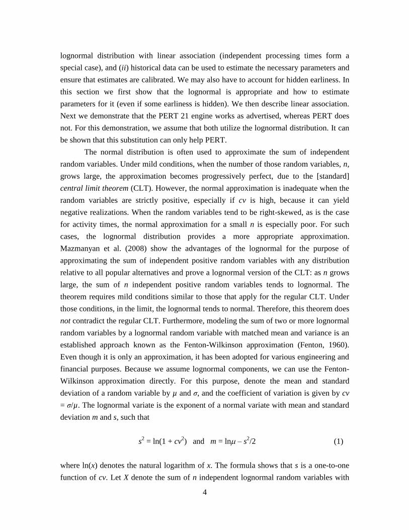
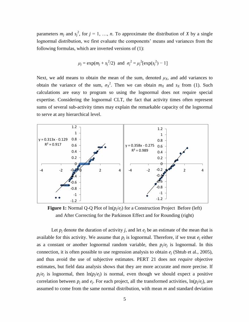
Figure 1: Normal Q-Q Plot of ln(pj/ej) for a Construction Project Before (left)

and After Correcting for the Parkinson Effect and for Rounding (right)

Let pj denote the duration of activity j, and let ej be an estimate of the mean that is

available for this activity. We assume that pj is lognormal. Therefore, if we treat ej either

as a constant or another lognormal random variable, then pj/ej is lognormal. In this

connection, it is often possible to use regression analysis to obtain ej (Shtub et al., 2005),

and thus avoid the use of subjective estimates. PERT 21 does not require objective

estimates, but field data analysis shows that they are more accurate and more precise. If

pj/ej is lognormal, then ln(pj/ej) is normal, even though we should expect a positive

correlation between pj and ej. For each project, all the transformed activities, ln(pj/ej), are

assumed to come from the same normal distribution, with mean m and standard deviation

y = 0.313x - 0.129R² = 0.917

-1.2

-1

-0.8

-0.6

-0.4

-0.2

0

0.2

0.4

0.6

0.8

1

1.2

-4 -2 0 2 4

y = 0.358x - 0.275R² = 0.989

-1.2

-1

-0.8

-0.6

-0.4

-0.2

0

0.2

0.4

0.6

0.8

1

1.2

-4 -2 0 2 4

6

s. The left side of Figure 1 shows a normal Q-Q plot of ln(pj/ej) for a residential

construction project. A normal Q-Q plot is obtained by sorting the data, pairing it with

scores that reflect the expected values of a sorted sample from a standard normal

distribution, and then fitting a regression line to the pairs. If the plotted points hug the

regression line closely, we say that the (normal) fit is good. The fit can be judged visually

(subjectively), but it can also be tested formally by various normality tests. Ignoring the

error term, a typical equation in such a regression, relating to the activity with the jth-

smallest ln(p/e), has the form

j

j

je

pszm lnˆˆ

where m and s are the regressed estimators of m and s, and zj = Φ−1

((j − 0.375)/(n +

0.25)); that is, the z-value for which the standard normal distribution cdf, Φ(z), yields a

probability of (j − 0.375)/(n + 0.25). Those particular probabilities are known as Blom's

scores (Blom, 1958), and their effectiveness is widely accepted. In other words, we treat

ordered ln(pj/ej) values as our dependent variables, and we obtain estimators for m and for

s. The slope is an estimate of s, the standard deviation of the internal normal variate

within the lognormal, and the intercept is an estimate of m. We adopt this approach

because it also works when the Parkinson effect is involved. The trend lines in the figure

are obtained by such regression. A useful test statistic for such a regression is R—the

square root of the ubiquitous R2 statistic—which is 0.958 in this example (because R

2 =

0.9178). For the particular sample size we employ, we can reject the normality

assumption for R < 0.987, so this sample is apparently not lognormal.

Now consider hidden earliness, also known as the Parkinson effect. If the

reported time matches the estimate perfectly, we obtain ln(pj/ej) = ln(1) = 0. Indeed, quite

a few points in the figure are 0. The Parkinson distribution is obtained when a fraction q

of all early points are reported "on-time" (q is the Parkinson propensity). In the example,

that is apparently the case. If we remove these points from the sample, use appropriate

averages for tied points and trim the sample so that the proportion of tardy points is

correct, we obtain the Q-Q plot on the right, which passes the normality test easily. Thus,

we must address two issues before normality of the log-transformed data is clearly

revealed: a large cluster of points with a logarithm of zero—indicating a sizable

Parkinson propensity—and similar but smaller clusters due to rounding. (Formally, this

sample could pass the normality test, albeit marginally, even without the second

7

correction.) We suspect that such difficulties have been obstacles to understanding that

processing times can be modeled very effectively as lognormal. Nonetheless, similar

evidence has been published before for cases without the Parkinson effect (for instance,

May et al., 2000; Strum et al., 2000; Lipke, 2002).

We say that a series of positive random variables {Yj}j=1,...,n is subject to linear

association if there exists a series {Xj}j=1,...,n of positive independent random variables and

an additional positive independent random variable, B, such that Yj = BXj (for j=1, ..., n).

Here B is a bias factor, also known as a systemic error or productivity factor, and because

it is shared by all Yj values it induces positive correlation between them (Trietsch,

2005a). Under the independence assumption, the coefficient of variation for the length of

a serial project tends to zero as the number of activities grows large, but under linear

association it tends to the coefficient of variation of B. If Xj and B are lognormal, then so

is Yj. To see that, take logarithms and the statement is that the sum of normal variates is

normal. It can be shown that the converse is also true: if Yj is lognormal and Yj = BXj,

then both B and Xj must be lognormal. The lognormal CLT is equally useful for linearly

associated processing times even though they are not independent. We just have to add

up the elements Xj before multiplying by B; that multiplication simply involves adding up

logarithms—which are normally distributed—and then taking the exponent. In more

qualitative terms, linear association implies that each project has its own mean, and

potentially also its own standard deviation. Nonetheless, linear association also allows

independence as a special case. B plays two important roles in PERT 21: (i) when

estimated from history, it provides calibration; and (ii) it assures that safety buffers do not

become negligible for large projects, which is the most pernicious result of the

independence assumption.

If projects can indeed be modeled well by linear association and lognormal

distributions, then projects can have different average time consumption levels than what

should be expected under the PERT independence assumption. There is ample evidence

that projects often have time consumption differences that cannot be explained under the

independence assumption but can be modeled well by linear association. Data from two

families of five and nine projects obtained by Gevorgyan (2008) can be used to

demonstrate these points, as depicted on the left sides of Figures 2 and 3 (from Trietsch et

al., 2011). The data includes original estimates and subsequent realizations for all

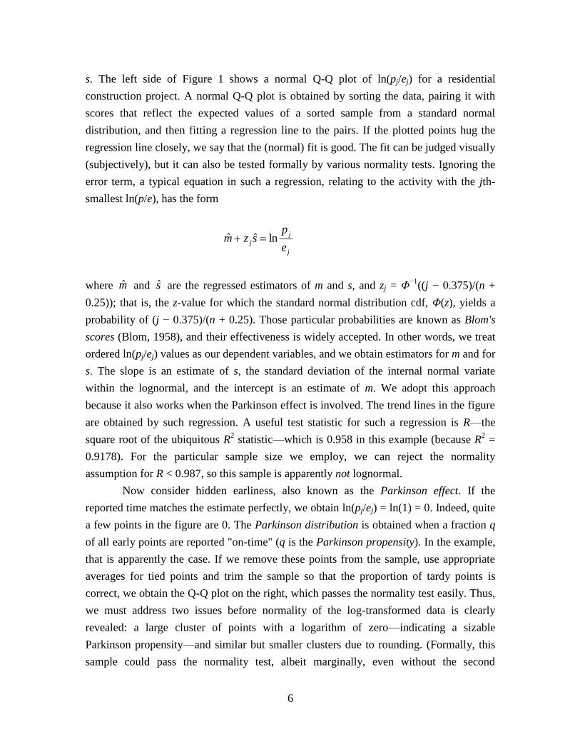
activities in these projects. The left hand side of Figure 2, which concerns the nine-

project family, is based on the assumption that the activities in each project are

independent and that the estimates are not biased. For each project the PERT

independence assumption is invoked to estimate the distribution of the sum of all activity

8

times—that is, the project duration if it were serial—and the probability of the actual sum

under this probability is calculated. This is done, in this case, under the assumption that

cv is the same under PERT and PERT 21, but in the PERT case there is also an

assumption that the estimated mean is correct for all projects. Let Fk(t) denote the

cumulative distribution function (cdf) of project k, and let Ck denote the actual combined

time of all activities in project k, then Fk(Ck) is the probability that the sum of all

activities would not exceed the actual sum, Ck. Under the PERT independence

assumption, the set of all Fk(Ck) values for k = 1, ..., 9 should be a random sample from a

standard uniform distribution. By testing whether they behave like such a sample, we can

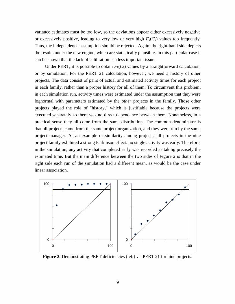
test the independence assumption. That can be done visually and formally by a P-P plot.

A P-P plot (also known as a P-P chart) is a special case of a Q-Q plot, where the

distribution tested is uniform. It is depicted within a unit square where the main diagonal

represents the standard uniform distribution, U[0, 1]. By plotting the sorted values from

the sample on the vertical scale against their approximate expected location under the

standard uniform distribution we can visually judge the fit. Formal tests such as the

Kolmogorov-Smirnov (K-S) test can also be used. The left side of Figure 2 is such a P-P

plot, and a formal K-S test rejects the hypothesis that it is a random sample from a

standard uniform distribution with a very high significance: the p-value—that is, the

probability of obtaining such a result by chance when the distribution is indeed U[0, 1]—

is below 0.0005. If we were to set due dates such that under PERT the project should

complete on time with a probability of 90%, then eight out of nine projects would fail

(see the horizontal line at 0.9 in the figure). In other words, setting due dates by the PERT

approach would fail miserably. Compare these results visually to the right side of Figure

2, where due dates with a service level of 90% would suffice in eight cases out of nine;

that is, due dates would provide the service level they are designed to provide. That part

of the figure is based on the stochastic engine in PERT21, as we elaborate below. For

these projects, it can be shown that the problem with the left side is due both to the

independence assumption and to consistent optimistic bias in the estimates, but mainly to

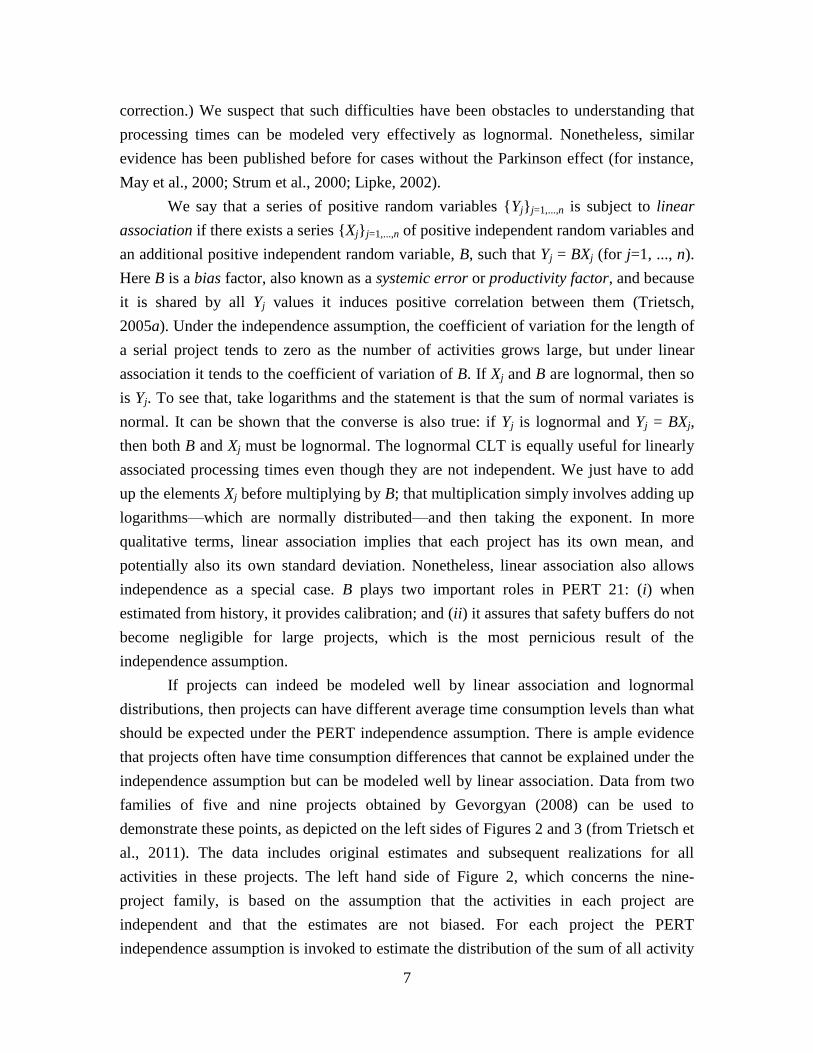
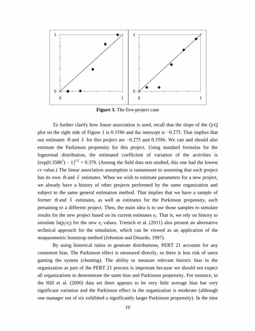
the latter. Similarly, the left side of Figure 3 depicts the results for the five-project family.

Here it is clear that too many projects have very low or very high Fk(Ck) values. In

particular, after sorting, those values are given by

{0.0009, 0.0071, 0.3883, 0.8320, 0.9968}

That is, three values out of five are either below 1% or above 99%, which is a highly

unlikely outcome under the independence assumption. Some reflection reveals that the

9

variance estimates must be too low, so the deviations appear either excessively negative

or excessively positive, leading to very low or very high Fk(Ck) values too frequently.

Thus, the independence assumption should be rejected. Again, the right-hand side depicts

the results under the new engine, which are statistically plausible. In this particular case it

can be shown that the lack of calibration is a less important issue.

Under PERT, it is possible to obtain Fk(Ck) values by a straightforward calculation,

or by simulation. For the PERT 21 calculation, however, we need a history of other

projects. The data consist of pairs of actual and estimated activity times for each project

in each family, rather than a proper history for all of them. To circumvent this problem,

in each simulation run, activity times were estimated under the assumption that they were

lognormal with parameters estimated by the other projects in the family. Those other

projects played the role of "history," which is justifiable because the projects were

executed separately so there was no direct dependence between them. Nonetheless, in a

practical sense they all come from the same distribution. The common denominator is

that all projects came from the same project organization, and they were run by the same

project manager. As an example of similarity among projects, all projects in the nine

project family exhibited a strong Parkinson effect: no single activity was early. Therefore,

in the simulation, any activity that completed early was recorded as taking precisely the

estimated time. But the main difference between the two sides of Figure 2 is that in the

right side each run of the simulation had a different mean, as would be the case under

linear association.

Figure 2. Demonstrating PERT deficiencies (left) vs. PERT 21 for nine projects.

0

100

0 100

0

100

0 100

10

Figure 3. The five-project case

To further clarify how linear association is used, recall that the slope of the Q-Q

plot on the right side of Figure 1 is 0.3586 and the intercept is −0.275. That implies that

our estimates m and s for this project are −0.275 and 0.3586. We can and should also

estimate the Parkinson propensity for this project. Using standard formulas for the

lognormal distribution, the estimated coefficient of variation of the activities is

[exp(0.35862) – 1]

1/2 = 0.370. (Among the field data sets studied, this one had the lowest

cv value.) The linear association assumption is tantamount to assuming that each project

has its own m and s estimates. When we wish to estimate parameters for a new project,

we already have a history of other projects performed by the same organization and

subject to the same general estimation method. That implies that we have a sample of

former m and s estimates, as well as estimates for the Parkinson propensity, each

pertaining to a different project. Then, the main idea is to use those samples to simulate

results for the new project based on its current estimates ej. That is, we rely on history to

simulate ln(pj/ej) for the new ej values. Trietsch et al. (2011) also present an alternative

technical approach for the simulation, which can be viewed as an application of the

nonparametric bootstrap method (Johnston and Dinardo, 1997).

By using historical ratios to generate distributions, PERT 21 accounts for any

consistent bias. The Parkinson effect is measured directly, so there is less risk of users

gaming the system (cheating). The ability to measure relevant historic bias in the

organization as part of the PERT 21 process is important because we should not expect

all organizations to demonstrate the same bias and Parkinson propensity. For instance, in

the Hill et al. (2000) data set there appears to be very little average bias but very

significant variation and the Parkinson effect in the organization is moderate (although

one manager out of six exhibited a significantly larger Parkinson propensity). In the nine

0

1

0 1

0

1

0 1

11

projects depicted in Figure 2 there is a high optimistic bias in estimates as well as high

variation and a very high Parkinson propensity. The five project case exhibits a moderate

optimistic bias and a moderate Parkinson propensity. PERT 21 is capable of providing

the correct response to each of these cases. (For future reference we note that none of the

field data sets exhibited pessimistic bias. That contradicts a crucial CCPM assumption.)

PERT 21 end-users are not required to supply more complex input than CPM or

CCPM users, provided there is access to historical data. That requirement is not onerous

because we are recommending the new engine for existing project management DSS,

which should already have the necessary historical information in their database.

Nonetheless, PERT 21 can also be used without organizational history, because we can

use generic history from the relevant industry until enough organizational information

becomes available over the course of time. However, the use of generic data instead of

organizational data tends to involve high variance estimates, because generic data also

reflect variance between organizations. That increase is not caused by PERT 21:

executing a project without sound historical data is inherently more risky and PERT 21

just reflects that. In terms of direct user input, there is no difference between PERT 21

and CPM or CCPM. In terms of output, PERT 21 differs from CPM or CCPM by

providing stochastic information. We discuss how that information can be presented and

potentially used for control in the next two sections.

3. Stochastic Sequencing, Scheduling and Crashing

Highly stylized models for the resource constrained project scheduling problem

(RCPSP) typically address a single hierarchical level with deterministic processing times

and a constant renewable resource profile throughout the project duration. Furthermore—

for tractability—they focus on the makespan (project duration) objective and rarely

address crashing. Given such a model, sequencing to minimize makespan is the correct

approach to resource leveling because the true purpose of resource leveling is to

minimize resource idleness—or wasted flowtime cost, but we achieve that for any given

resource level by minimizing the makespan. We may wish to experiment with different

resource levels, however, to select the best compromise between makespan and resource

cost, which is essentially a form of crashing. Even such highly stylized RCPSP models

are very complex mathematically, so extensions to more realistic formulations are few.

However, once we realize that heuristics are the only practical way to proceed, we might

as well address more realistic objectives and more realistic scenarios. First and foremost,

we should address stochastic variation (Herroelen and Leus, 2005). We should also

12

consider resources more explicitly. With this in mind, we now discuss the structure and

guiding principles of scheduling under PERT 21.

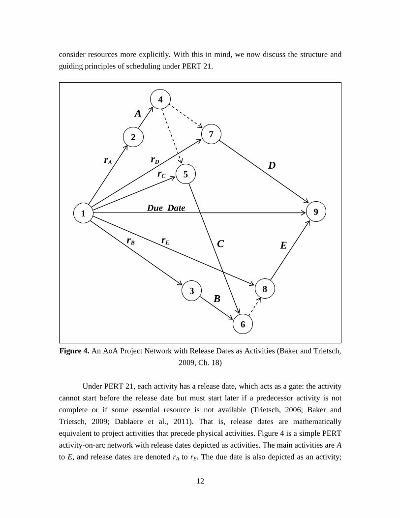
Figure 4. An AoA Project Network with Release Dates as Activities (Baker and Trietsch,

2009, Ch. 18)

Under PERT 21, each activity has a release date, which acts as a gate: the activity

cannot start before the release date but must start later if a predecessor activity is not

complete or if some essential resource is not available (Trietsch, 2006; Baker and

Trietsch, 2009; Dablaere et al., 2011). That is, release dates are mathematically

equivalent to project activities that precede physical activities. Figure 4 is a simple PERT

activity-on-arc network with release dates depicted as activities. The main activities are A

to E, and release dates are denoted rA to rE. The due date is also depicted as an activity;

Due Date

D

E C

B

A

rE

rD

rC

rA

rB

6

9

8 3

1

5

2 7

4

13

indeed the due date is mathematically equivalent to a release date, as it is the release date

for the project completion event. Dummy activities are depicted by dashed arrows. All

activities have release dates (although rA and rB may be set to zero).

Release dates are set for a given project network, but for the purpose of

scheduling release dates we assume that the network incorporates soft precedence

constraints that enforce sequencing decisions. That is, the network is feasible in the sense

that it accounts for resource constraints. When viewed this way, the purpose of

sequencing is essentially to select a good network from a large set of feasible networks.

Currently, the state of the art for scheduling with holding costs as well as resource costs

is based on neighborhood search techniques that can be applied for both deterministic and

stochastic times. The former are quicker, the latter more relevant. A good compromise is

to start with a deterministic model and account for the main stochastic aspects

subsequently. Sequencing heuristics are covered in more detail by Baker and Trietsch

(2009). Here, for the purpose of setting release dates, we focus on scheduling with

stochastic processing times for a given sequence. That is, we assume a network is given

with soft constraints based on previous sequencing decisions as necessary to satisfy

resource constraints. However, we show that the flowtime models we present for

scheduling release dates can also be used to guide sequencing decisions.

In a nutshell, the correct objective of sequencing, scheduling and crashing is to

minimize the total expected flowtime costs that a project incurs. Crashing fits this

framework because it reduces total expected flowtime costs by judiciously increasing

them for selected critical activities. The project makespan—the classic RCPSP

objective—is typically the single most important flowtime, but it is not the only one. In

addition, we have to consider the holding cost of complete activities—which includes the

holding cost of incorporated consumable resources (such as materials and budgetary

expenditures) and the time value (or hiring costs) of renewable resources (such as

workers and equipment) necessary to execute the project. Tardiness cost is often

expressed as a penalty that is proportional to the tardiness, in which case it is possible to

model it as a flowtime cost.

The correct accounting for resources depends to a large extent on organizational

structure. The RCPSP implicitly assumes a stand-alone project or, essentially, a pure

project organization where each project is managed independently and renewable

resources are often duplicated (Shtub et al., 2005). That is, resources are dedicated to the

project and serve multiple activities within the project. If we assume dedicated resources

are carried from project start (time zero) to completion, these costs are minimized by

minimizing the makespan. In general, dedicated resources may have to idle between

14

activities and, under the basic model, that idleness is minimized by minimizing the

makespan. Makespan minimization also achieves the best possible resource leveling,

although for that purpose we may wish to compare different resource profiles and select

the best one. But if we recognize that some resources—including dedicated ones—can be

inducted after time zero or released before project completion, then sequencing should

take resource idleness into account explicitly: it can be reduced by starting the first

activity that requires a resource late or by finishing the last such activity early.

Incidentally, under this scenario, resource leveling is no longer an important objective

except in cases where congestion is an issue. In summary, by ignoring resource induction

and release times, conventional models miss out on an important need.

By contrast, in a pure functional organization resources are allocated to single

activities, so we may think of them as temporary. As a first approximation, we can then

say that resource cost is not a function of sequencing and therefore it can be treated as a

constant, and thus ignored. Idleness is then an issue for central management—above the

project level—but expected idleness cannot be reduced without increasing expected

queueing delays to projects. Sound capacity management principles imply that enough

capacity should be available to balance the cost of idleness with the cost of queueing

(Trietsch and Quiroga, 2009). Matrix organizations are in between: some resources are

dedicated, others temporary. In what follows, for generality, we assume that both

dedicated and temporary resources are scheduled. In either case, resource time value

often dominates other flowtime costs, especially when we use capital intensive

technology to reduce the total cost of an activity or to crash it: that would imply activities

take a short time but incur a high daily charge while they last; once complete, their main

holding cost is interest on the total cost, which is typically much smaller. The upshot of

all this is not only that resourcing decisions and sequencing decisions depend on each

other but also that before an activity starts we must induct all consumable resources for it

and we may also have to induct renewable resources. In such cases, the activity's release

date is effectively a due date for the staging operation. But staging operations are rarely

modeled explicitly by the main project network. In other words, staging is managed on a

lower hierarchical level, and upper-level release dates act as lower level due dates. If we

recognize that financial funds are also resources that have to be staged, we can see that

each activity requires its own release date to make possible scheduling at the lower level.

Furthermore, the earliest release date of a successor activity acts as a de facto due date for

predecessor activities; that is, every activity has its own release date (possibly zero) and

due date.

15

In more technical terms, consider the following deterministic model. A project

consists of n activities and has a due date (d). Each activity incurs an earliness cost per

unit time denoted αj for activity j (here and henceforth j = 1, 2, ..., n), and define α = α1 +

α2 + ... + αn. Earliness costs reflect the economic value of postponing activities; that is,

they are holding costs. Thus, we have an incentive to postpone the start of each activity to

avoid paying earliness cost. However, the project also incurs a tardiness cost per unit time

denoted β. In practice, tardiness cost reflects the delay in obtaining revenue and often

includes explicit compensation to customers when a due date is missed. The tardiness

penalty provides an incentive to start all activities early. Because both earliness and

tardiness costs apply, we should balance activities' earliness costs against the project’s

tardiness costs. To avoid starting activities too early, and thus incur excessive holding

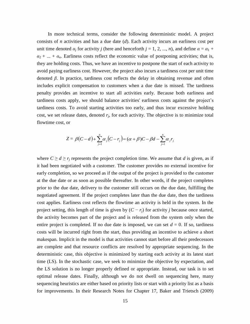
cost, we set release dates, denoted rj, for each activity. The objective is to minimize total

flowtime cost, or

Z =

n

j

jj

n

j

jj rdCrCdC11

)(

where C ≥ d ≥ rj represents the project completion time. We assume that d is given, as if

it had been negotiated with a customer. The customer provides no external incentive for

early completion, so we proceed as if the output of the project is provided to the customer

at the due date or as soon as possible thereafter. In other words, if the project completes

prior to the due date, delivery to the customer still occurs on the due date, fulfilling the

negotiated agreement. If the project completes later than the due date, then the tardiness

cost applies. Earliness cost reflects the flowtime an activity is held in the system. In the

project setting, this length of time is given by (C − rj) for activity j because once started,

the activity becomes part of the project and is released from the system only when the

entire project is completed. If no due date is imposed, we can set d = 0. If so, tardiness

costs will be incurred right from the start, thus providing an incentive to achieve a short

makespan. Implicit in the model is that activities cannot start before all their predecessors

are complete and that resource conflicts are resolved by appropriate sequencing. In the

deterministic case, this objective is minimized by starting each activity at its latest start

time (LS). In the stochastic case, we seek to minimize the objective by expectation, and

the LS solution is no longer properly defined or appropriate. Instead, our task is to set

optimal release dates. Finally, although we do not dwell on sequencing here, many

sequencing heuristics are either based on priority lists or start with a priority list as a basis

for improvements. In their Research Notes for Chapter 17, Baker and Trietsch (2009)

16

present a priority list tailored specifically for this objective function. This list prioritizes

activities with long expected durations and low αj values while accounting for

technological precedence constraints.

Putting aside the crashing option, activity durations are stochastic but not subject to

change by our decisions. However, by optimizing the release dates we can minimize our

objective function. In the stochastic case, the guiding principle for optimality is stochastic

balance. Because each and every activity has its own release date, and because every path

in the project starts with a release date, at least one release date must be critical; to be

able to say that, however, we count the due date as a release date, which is critical if and

only if the project completes on time. The criticality of the due date is also known as the

service level, because it is the probability the project will not be tardy. The probability the

critical path includes rj is the criticality of the jth release date, denoted qj. Stochastic

balance is achieved when we set rj in such a way that qj will be as close as possible to, but

not less than, αj/(α+β). Ideally, the project's service level is then β/(α+β), but that may be

impossible if the due date is too tight. In that case, some activities with no predecessors

acquire excessive criticality even if they start as early as possible. As a result, the project

service level is decreased. But the criticality of any release date that is not set to early

start should still match αj/(α+β). For discrete distributions, rounding should be upwards,

and it is possible for more than one activity to be critical at the same time. The

recommended way to find the correct release dates is by numerical search such that the

correct criticalities will be achieved for a sufficiently large simulated sample; that is, we

employ simulation-based optimization (SBO). This particular SBO application is highly

tractable, and can even be implemented as an Excel add-in.

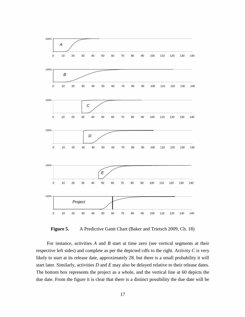
We can visually assess how a stochastic project subject to given release dates is

likely to perform by using a predictive Gantt chart (Baker and Trietsch, 2009), also

known as the stochastic Gantt chart (Dablaere et al., 2011). Figure 5 depicts a predictive

Gantt chart for the project of Figure 4, after balancing it stochastically for a particular set

of distributions and parameters. That is, the release dates in the figure are optimal. The

ability to read a predictive Gantt chart is the main skill required of a PERT 21 user that is

not already required for CPM (or CCPM). Essentially, a predictive Gantt chart uses cdfs

(cumulative distribution functions) instead of vertical lines to delimit the start and the end

of an activity. The height of each activity in this depiction is one, or 100%—because a

cdf starts at zero and is monotone increasing until it reaches one. Thus, the shape of an

activity in the chart is not rectangular, as it would be in a regular Gantt chart.

17

Figure 5. A Predictive Gantt Chart (Baker and Trietsch 2009, Ch. 18)

For instance, activities A and B start at time zero (see vertical segments at their

respective left sides) and complete as per the depicted cdfs to the right. Activity C is very

likely to start at its release date, approximately 28, but there is a small probability it will

start later. Similarly, activities D and E may also be delayed relative to their release dates.

The bottom box represents the project as a whole, and the vertical line at 60 depicts the

due date. From the figure it is clear that there is a distinct possibility the due date will be

A

B

C

D

E

Project

0

100

0 10 20 30 40 50 60 70 80 90 100 110 120 130 140

0

100

0 10 20 30 40 50 60 70 80 90 100 110 120 130 140

0

100

0 10 20 30 40 50 60 70 80 90 100 110 120 130 140

0

100

0 10 20 30 40 50 60 70 80 90 100 110 120 130 140

0

100

0 10 20 30 40 50 60 70 80 90 100 110 120 130 140

0

100

0 10 20 30 40 50 60 70 80 90 100 110 120 130 140

100%

100%

100%

100%

100%

100%

18

missed. That possibility is partly because the cost structure allows tardiness (with a

desired probability of α/(α+β) = 0.4) and partly because the due date is too tight (so the

actual tardiness probability is about 0.45). To elaborate, two activities (A and B) are

released at time zero, which suggests that in this example minimizing the objective

function is associated with a lower service level than would be achieved for a higher due

date.

One interesting feature of predictive Gantt charts is that certain areas represent

expected durations. The area enclosed by the start and finish cdf of each activity is the

expected activity duration (as in the deterministic case where both these cdfs are

represented by vertical lines). The area of the tail beyond the due date in the "project" bar

represents the expected project tardiness (approximately 6.5). The area of the wedge to

the left of the due date below the cdf is the expected earliness (about 3.5). The predictive

Gantt chart resembles the output of risk management modules, which also use cdfs. The

main difference is that a predictive Gantt chart has a cdf not only for project completion

but also for all activity start and finish times. (In addition to cdfs, risk modules output can

include histograms to represent the density function. It is straightforward to add density

functions to predictive Gantt charts as well.)

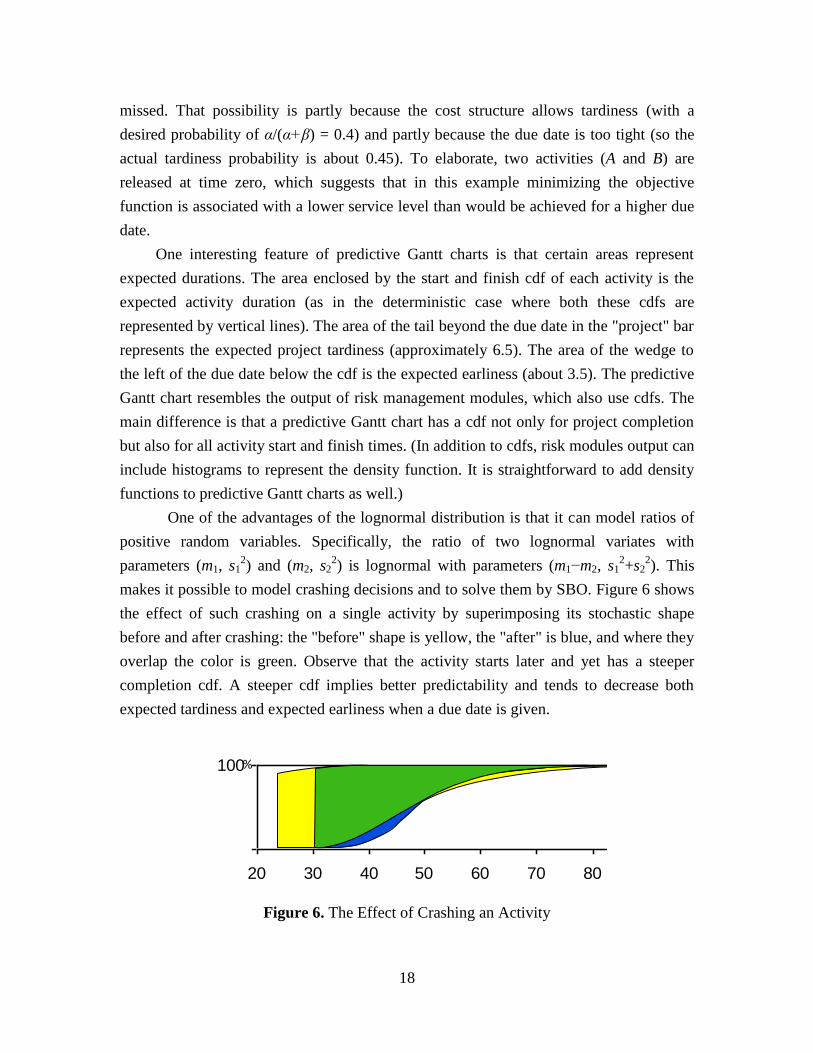
One of the advantages of the lognormal distribution is that it can model ratios of

positive random variables. Specifically, the ratio of two lognormal variates with

parameters (m1, s12) and (m2, s2

2) is lognormal with parameters (m1−m2, s1

2+s2

2). This

makes it possible to model crashing decisions and to solve them by SBO. Figure 6 shows

the effect of such crashing on a single activity by superimposing its stochastic shape

before and after crashing: the "before" shape is yellow, the "after" is blue, and where they

overlap the color is green. Observe that the activity starts later and yet has a steeper

completion cdf. A steeper cdf implies better predictability and tends to decrease both

expected tardiness and expected earliness when a due date is given.

Figure 6. The Effect of Crashing an Activity

0

100

20 30 40 50 60 70 80 90 100 110 120

%

19

As a rule, reducing the inherent variance in activity time is very difficult. One

should not confuse the provision of safety time with fundamental variance reduction:

safety time is a response to variance. One counterintuitive empirical exception highlights

the value of careful sequencing. We define a dense schedule as one where, if activities

take their expected time exactly, there is little idling. It turns out that dense schedules

tend to have not only a low mean but also a low variance relative to loose schedules. This

empirical observation contradicts a common intuitive error, often cited as an excuse to

forego careful sequencing, namely that a loose schedule is likely to lead to a more

protected and therefore better final schedule. In fact, however, simulation studies suggest

the opposite: dense schedules increase the Jensen gap but tend to decrease both the mean

and the variance of the total duration. If we account for the increased Jensen gap

correctly—which is automatic under PERT 21 because it uses simulation—the likely

final result of a dense schedule relative to a loose one is an improvement. For any desired

service level, due dates can be tighter and expected tardiness relative to these tighter due

dates is smaller. The intuitive error is due to ignoring the fact that most of the

"protection" provided by a loose schedule tends to be wasted, whereas increasing the

nominal critical path length unnecessarily increases the expected project length with

certainty.

4. Control and Delegation

Although our approach is static, we recognize that plans have to be updated

dynamically. Among other things, that implies that criticalities are expected to change

dynamically. Even if the plan is essentially unchanged, actual project performance is not

likely to adhere to the initial schedule or budget precisely. For the most part, we limit

ourselves to schedule control, subject to the assumption that our budget has a buffer that

allows us to take reasonable corrective actions to control the schedule. But the same

principles can also be used for budget control. In fact, the two are intertwined, because

schedule control affects budget consumption. We note, however, that data reported by

Lipke et al. (2009) in their Table 1 supports the notion that budget consumption is

approximately lognormal and subject to linear association. That dataset also shows a

positive correlation between schedule and budget performance ratios. This correlation is

not surprising: it suggests that some causes increase both time and expenditure and/or

that the organization's response to looming delays increases expenditure.

In general, we encounter two types of variation. The first is due to randomness of

processing times. We prepare for this type of variation and we depict it with a predictive

Gantt chart. If only that type of variation occurs, we may say, loosely, that the project is

20

under statistical control (which means that the variation is within statistically predictable

limits). Another type of variation is due to changes in plans or other "out of control"

events. That type of variation typically requires re-sequencing as well as re-scheduling of

release dates. By contrast, when the project is in statistical control, the safety time buffers

are designed to reduce the need to re-schedule and drastically reduce the need to re-

sequence.

For control, a good decision support system must (i) provide a clear signal when a

correction is required, (ii) facilitate the interactive determination of an approximately

correct response, (iii) provide a check on the new plan, and (iv) update the plan once the

proposed change is accepted by the user. Most existing project management software

does not even begin to provide these capabilities, although CCPM addresses the first

point by monitoring buffer consumption. A new plan is often required when the project

scope is changed, or when it becomes clear that the original plan is no longer viable; for

instance, if an important development fails and we must use a different approach.

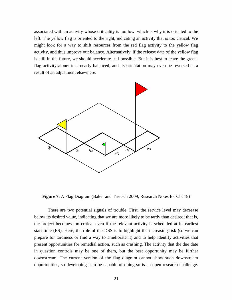
The flag diagram is designed specifically to provide graphical signals showing the

magnitude and orientation of deviations from balance that are not due to scope change

etc. Thus, it supports these DSS requirements. The flag diagram interprets the

distributional information of the predictive Gantt chart and provides signals that help

users focus attention where it is most cost-effective and needed. Figure 7 illustrates: for

each activity, a rectangle (shown as a parallelogram) depicts the criticality and the

normalized marginal holding cost (that is, we scale costs so that α + β = 1). Any of these

rectangles could represent the project's due date performance, in which case we would

replace αj by β and qj by the service level. If the normalized cost and the criticality are

equal (that is, the rectangle is a square), the activity is in perfect stochastic balance.

Otherwise, flags whose height is proportional to the marginal opportunity that can be

obtained by rebalancing are used to highlight which of the activities are most out of

balance. In our context, the activities whose criticalities sum to one are ongoing activities,

any future activities that we wish to include explicitly, and all other activities (including

the due date) may be represented by one rectangle; that last rectangle represents the event

that none of the current activities is critical, so the critical activity must either be the due

date or an un-depicted future activity. The color scheme in the figure is determined

somewhat arbitrarily as a function of the marginal gain available by providing balance;

that is, tall flags are red, short ones are green. The tallness of a flag depends entirely on

the ratio between the sides of its rectangle. The size of a flag is also important because it

provides partial evidence on the size of the opportunity. The size is a function of the

absolute difference between the sides. The red flag in this particular example is

21

associated with an activity whose criticality is too low, which is why it is oriented to the

left. The yellow flag is oriented to the right, indicating an activity that is too critical. We

might look for a way to shift resources from the red flag activity to the yellow flag

activity, and thus improve our balance. Alternatively, if the release date of the yellow flag

is still in the future, we should accelerate it if possible. But it is best to leave the green-

flag activity alone: it is nearly balanced, and its orientation may even be reversed as a

result of an adjustment elsewhere.

Figure 7. A Flag Diagram (Baker and Trietsch 2009, Research Notes for Ch. 18)

There are two potential signals of trouble. First, the service level may decrease

below its desired value, indicating that we are more likely to be tardy than desired; that is,

the project becomes too critical even if the relevant activity is scheduled at its earliest

start time (ES). Here, the role of the DSS is to highlight the increasing risk (so we can

prepare for tardiness or find a way to ameliorate it) and to help identify activities that

present opportunities for remedial action, such as crashing. The activity that the due date

in question controls may be one of them, but the best opportunity may be further

downstream. The current version of the flag diagram cannot show such downstream

opportunities, so developing it to be capable of doing so is an open research challenge.

q1 α1 q2

α2

q3 α3

22

The second type of signal occurs when an activity is delayed sizably beyond its release

date so that the project due date performance is at excessive risk (again). If other

activities are available for processing on the resources that are idle due to the delay, it

may be beneficial to dispatch another activity ahead of its turn. Here the role of the DSS

is to alert the user to the problem and to the opportunity. In this case it is necessary to

estimate how long the delay is likely to continue and to assess the cost and benefit of the

proposed change.

Our control methodology is based on analyzing criticalities and responding to

signals based on unbalanced criticalities. The flag diagram helps focus on critical

activities that are out of balance and thus it also tells us which activities do not require the

same level of attention yet. Now consider that a reasonable manager may not be able to

coordinate more than about seven different entities. It would make sense for a project

manager to focus on the five to seven most important activities. To prevent problems

from developing in the other activities, responsibility for them should be delegated. For

whoever is responsible for those less important activities, they can be sorted in much the

same way and some of them may be delegated further. If the criticality of an initially

unimportant activity increases substantially, however, it may become sufficiently acute to

require handling by the higher hierarchical level after all. Thus, if we choose to use this

approach, the allocation of responsibility for activities is hierarchical and to some extent

flexible.

Good risk modules already show how to focus attention on important risk causes

by using a Tornado diagram. Such diagrams are essentially equivalent to Pareto charts

and they rely on sensitivity analysis. However, Tornado diagrams do not take cost into

account, and thus they may focus attention on activities that may be important but

difficult to change, and draw attention away from the most cost-effective opportunities if

they don't happen to be large. Further research is required to include cost considerations

in Tornado diagrams and to compare their performance with flag diagrams.

5. Risk Modules and CCPM

Having described the structure and the capabilities of PERT 21, we now compare

it with two established alternatives: (i) risk modules, and (ii) CCPM. Starting with risk

modules, the first requirement is to list all the "known unknowns," which are risk events

that experience suggests may repeat. Each of these known unknowns is then assigned a

probability and its potential effect must be sized. As implemented, those tasks require

subjective inputs. Furthermore, the default assumption is that risks are independent: users

are required to specify correlations if they reject the independence assumption.

23

Technically, they might do that by estimating correlation coefficients, but there is no

established methodology how to do it. In general, it is very difficult to provide valid

correlations unless we take the PERT 21 approach, where the systemic error, B, which is

regressed from historic data, provides objective information on correlations. Thus, risk

modules share the two major problems with PERT, namely the elicitation of subjective,

often uncalibrated, estimates and the insufficient accounting for correlations. We already

showed evidence that those are indeed problems. In addition, Tversky and Kahneman

(1974) point out that expert estimates are subject to very sizable optimistic bias: on

average, subjective confidence intervals of 98% only hold 70% of possible outcomes.

Woolsey (1992) points out that eliciting triplet-estimates is onerous and therefore often

frivolous. Those problems are inherited by the subjective estimates and the need to

estimate effects and probabilities for risk modules. However, just listing the known

unknowns is beneficial as part of contingency planning. Risk registers are also useful for

allocation of responsibility: bad outcomes that were duly recorded in the register are not

the responsibility of the project manager (Zwikael and Smyrk, 2011). As for "unknown

unknowns," they are typically addressed by arbitrary buffers called "management

reserves." By contrast, PERT 21 specifies data-based reserves that are optimal in terms of

minimizing flowtime costs, as we discussed in the former section. But the idea that at

least some unknowns justify protection is common to both. Finally, it should be possible

to adapt the history-based approach of PERT 21 to improve the performance of risk

modules, so PERT 21 is not in conflict with risk modules. However, risk modules are not

universally implemented, perhaps because they are too complex, and PERT 21 can

preempt them where they are not justified.

Having said all that, we should clarify that knowledgeable users can achieve

results that are very similar to PERT 21 by risk analysis and simulation. To mention one

successful approach of this type, Cates and Mollaghasemi (2007) describe a scheduling

application at NASA for the International Space Station program. They use historical

data extensively and do not make the independence assumption. NASA is a quintessential

project organization, yet historical data proved useful for estimating activity distributions

(including correlations) and for feeding simulation models. In effect, PERT 21 just

simplifies the analysis with the aim to make it accessible to less sophisticated users as

well. For a different perspective on practice at NASA, however, see Butts and Linton

(2009).

Some parallels exist between PERT 21 and CCPM. Specifically, they both use

release dates designed to provide explicit or implicit safety buffers. CCPM's main

attractions are simplicity of use, explicit protection against stochastic variation, and a set

24

of reasonable control guidelines. It is well known, however, that it suffers from major

weaknesses (Herroelen et al., 2002; Raz et al., 2003). Trietsch (2005b) critiques

numerous issues about CCPM as presented by Goldratt (1997). He also observes that the

advent of CCPM should be interpreted as a call for a more holistic approach to project

scheduling and lists several technical issues that must be addressed for that purpose.

Addressing that list has been part of the development of PERT 21. CCPM is based on an

earlier source—Pittman (1994)—but with several enhancements. In a nutshell, Pittman's

work is insightful but incomplete. Goldratt presents a more complete framework, but

does so by violating reliability and relevance requirements. Some, but not all, of these

violations could be explained as practical compromises intended to simplify the

framework (and thus make it more attractive to potential adopters). In this connection,

PERT 21 sets buffers implicitly, by optimizing release dates, whereas CCPM sets them

explicitly. The PERT 21 approach is the correct one, but that is not a major issue. A much

more serious problem is that CCPM calls for halving the original estimates before using

half of the cuts as buffers. That is, instead of stochastic analysis, CCPM takes arbitrary

and reckless steps, which would only be acceptable if all projects were estimated

pessimistically. In fact, the reverse is often the case. Specifically, CCPM would fail in all

the field examples studied by Trietsch et al. (2011). PERT 21 addresses all these issues,

and does so in a manner that supports hierarchical application, whereas CCPM is based

on an implicit assumption that a single project network provides all the necessary detail.

To wit, CCPM does not specify release dates for all activities, thus ignoring the need to

prepare materials and other resources for them. That need, however, is well understood in

hierarchical project scheduling approaches (Kelley and Walker, 1959): in realistic

hierarchical projects practically every activity requires preparation and the earliest release

date of successor activities acts as a de facto due date.

6. Conclusion

Stochastic scheduling of projects remained essentially unsolved for over half a

century because of several persisting errors. First and foremost, the PERT independence

assumption is highly misleading and the lack of calibration is very risky, but other

problems that are in fact more minor—such as the Jensen gap—commanded more

attention in the research literature. State of the art risk analysis modules can overcome

these problems but that requires sound statistical analysis of past performance; PERT 21

automates such analysis at a basic level. The observation that few if any project

organizations employ statisticians to analyze past data and use it to help predict future

25

performance is anecdotal evidence that the need for sound analysis is often observed in

the breach.

We propose a new stochastic engine based on lognormal distributions with linear

association. Parameters for these distributions—even when they are also subject to the

Parkinson effect—are easy to estimate based on history of past estimates. With this

engine in place, users need not be expert statisticians to obtain useful and realistic

distributions. Using such distributions we can balance the criticalities of project activities

and we can control projects by monitoring that stochastic balance. The approach is easy

to implement in realistic hierarchical systems. To that end, we also presented two

contemporary graphical tools: predictive Gantt charts and flag diagrams. The former is a

useful way to show the results of stochastic analysis in a way that is easy to understand

with minimal training. The latter provides focusing signals that support control and help

delegate responsibilities in a flexible hierarchical manner. Our new engine can be easily

retrofitted into existing frameworks, so it does not require scrapping the huge investment

in existing project scheduling software. We replace only the deterministic assumption of

CPM or the flawed stochastic engine of PERT by the new engine, which can be

implemented with or without the new control approach.

More research and development is important. In principle, PERT 21 can be

implemented in parallel to existing risk modules, which are especially useful for

documenting known risks and for contingency planning. Furthermore, the PERT 21

estimation approach by history can be applied to assess risk event probabilities and

correlations: that aspect of risk modules is largely subjective at present and the generic

evidence is that subjective risk estimates are not reliable. The exact details of this

application require further research, however. Another important research area arises

because until now, there has not been a serious attempt to combine the CPM optimization

approach with the PERT stochastic modeling approach. The new engine makes such an

adaptation possible. That is, sequencing and crashing models developed under the

deterministic assumption can and should be adapted for stochastic times, thus achieving a

true marriage between PERT and CPM. Initial models along these lines have already

been identified or developed by Baker and Trietsch (2009, Chs. 17 and 18), and see also

Dablaere et al., (2011). Furthermore, models for ongoing estimation of criticalities during

the control phase still need to be developed and vetted. Another research direction

concerns project organizations. They need to coordinate multiple projects whereas we

mainly addressed a single project. In other words, we may have to solve a higher level

problem that is very similar to the job shop problem. None of the existing approaches to

this problem accounts for stochastic variation properly yet. Nonetheless, the state of the

26

art in dynamic job shop scheduling suggests that such sequencing decisions should be

guided by activity due dates (Baker and Trietsch 2009, Ch. 15). Under PERT 21, activity

due dates are effectively determined by subsequent release dates that depend on them.

Furthermore, the optimal criticality of those subsequent release dates can also provide

weights that can be used for prioritization. The effect of organizational structure on

project scheduling that we presented in Section 3 also requires more research. Other

important research directions are modeling the response to dynamic changes better,

identifying the best response to control problems, optimizing the capacity of project

organizations in a manner that will balance capacity costs and queueing costs, sequencing

models that take resource cost into account without the constant profile assumption, and

so on. Nonetheless, basic versions of the new engine and the new control approach are

ready for implementation right now.

Acknowledgement: We are grateful to Vladimir Liberzon (R&D Director, Spider Project

Team) for useful comments on a precursor of this paper.

References

Ash, R.C. and Pittman, P.H., 2008. Towards holistic project scheduling using critical

chain methodology enhanced with PERT buffering. International Journal of

Project Organisation and Management 1(2), 185-203.

Baker, K.R., Trietsch, D., 2009. Principles of Sequencing and Scheduling, John Wiley &

Sons, New York. (For Research Notes, see: http://mba.tuck.dartmouth.edu/pss/.)

Blom, G., 1958. Statistical Estimates and Transformed Beta Variables, John Wiley &

Sons, New York.

Butts, G., Linton, K., 2009. The Joint Confidence Level Paradox: A History of Denial.

White paper presented at NASA Cost Symposium, April 28th.

Cates, G.R., Mollaghasemi, M., 2007. The project assessment by simulation technique.

Engineering Management Journal 19(4), 3-10.

Clark, C.E., 1961. The greatest of a finite set of random variables. Operations Research 9,

145-162.

Dablaere, F., Demeulemeester, E., Herroelen, W., 2011. Proactive policies for the

stochastic resource-constrained project scheduling problem. European Journal of

Operational Research. doi:10.1016/j.ejor.2011.04.019.

Dodin, B., 1985. Bounding the project completion time distribution in PERT networks.

Operations Research 33, 862-881.

27

Fenton, L., 1960. The Sum of Log-Normal Probability Distributions in Scatter

Transmission Systems. IRE Transactions on Communication Systems 8(1), 57-67.

Gevorgyan, L., 2008. Project duration estimation with corrections for systemic error.

Unpublished master thesis, Industrial Engineering & Systems Management,

College of Engineering, American University of Armenia, Yerevan, Armenia.

Goldratt, E.M., 1997. Critical Chain. North River Press, Great Barrington, MA.

Herroelen, W., Leus, R., 2005. Project scheduling under uncertainty: Survey and research

potentials. European Journal of Operational Research 165, 289–306.

Herroelen, W., Leus, R., Demeulemeester, E., 2002. Critical Chain project scheduling:

Do not oversimplify. Project Management Journal 33(4), 48-60.

Hill, J., Thomas, L.C., Allen, D.E., 2000. Experts’ estimates of task durations in software

development projects. International Journal of Project Management 18, 13-21.

Johnston, J., Dinardo, J., 1997. Econometric Methods, Fourth Edition, McGraw-

Hill/Irwin, New York.

Kelley, J.E., Walker, M.R., 1959. Critical path planning and scheduling. Proceedings of

the Eastern Joint Computer Conference, Boston, pp. 160-173.

Kelley, J.E., 1961. Critical-path planning and scheduling: Mathematical basis. Operations

Research 9(3), 296-320.

Kelley, J.E., 1963. The critical path method: Resources planning and scheduling,"

Chapter 21 in Muth, J., Thompson, G.L., Industrial Scheduling, Prentice-Hall,

347-365.

King, W.R., 1971. Network simulation using historical estimating behavior. IIE

Transactions 3(2), 150-155.

Lipke, W., 2002. A study of the normality of earned value management indicators.

Measurement News 1-16.

Lipke, W., Zwikael, O., Henderson, K., Anbari, F., 2009. Prediction of project outcome:

The application of statistical methods to earned value management and earned

schedule performance indexes. International Journal of Project Management 27,

400-407.

Malcolm, D.G., Roseboom, J.H., Clark, C.E., Fazar, W., 1959 Application of a technique

for a research and development program evaluation. Operations Research 7, 646-

669.

May, J.H., Strum, D.P., Vargas, L.G., 2000. Fitting the lognormal distribution to surgical

procedure times. Decision Sciences 31, 129-148.

28

Mazmanyan, L., Ohanyan, V., Trietsch, D., 2008. The lognormal central limit theorem

for positive random variables. (Working Paper. Reproduced within the Research

Notes for Appendix A in http://mba.tuck.dartmouth.edu/pss/.)

Pittman, P.H., 1994. Project management: A more effective methodology for the

planning & control of projects. Unpublished doctoral dissertation, University of

Georgia.

Raz, T., Barnes, R., Dvir, D., 2003. A critical look at Critical Chain project management.

Project Management Journal 34(4), 24-32.

Schonberger, R.J., 1981. Why projects are 'always' late: A rationale based on manual

simulation of a PERT/CPM network. Interfaces 11, 66-70.

Shtub, A., Bard, J.F., Globerson, S., 2005. Project Management: Processes,

Methodologies, and Economics, 2nd ed, Pearson Prentice Hall, Upper Saddle

River, NJ.

Strum, D.P., Sampson, A.R., May, J.H., Vargas, L.G., 2000. Surgeon and type of

anesthesia predict variability in surgical procedure times. Anesthesiology 92,

1454–1466.

Trietsch, D., Mazmanyan, L., Gevorgyan, L., Baker, K.R., 2011. Modeling activity times

by the Parkinson distribution with a lognormal core: Theory and validation.

European Journal of Operational Research. doi:10.1016/j.ejor.2011.07.054.

Trietsch, D., 2005a. The effect of systemic errors on optimal project buffers.

International Journal of Project Management 23, 267–274.

Trietsch, D., 2005b. Why a critical path by any other name would smell less sweet: Towards

a holistic approach to PERT/CPM. Project Management Journal 36(1), 27-36.

Trietsch, D., 2006. Optimal feeding buffers for projects or batch supply chains by an

exact generalization of the newsvendor model. International Journal of Production

Research 44, 627-637.

Trietsch, D., Quiroga, F., 2009. Balancing stochastic resource criticalities hierarchically

for optimal economic performance and growth. Quality Technology and

Quantitative Management 6(2), 87-106.

Tversky A., Kahneman, D., 1974. Judgment under uncertainty: Heuristics and biases.

Science 185, 1124-1131.

Van Slyke, R.M., 1963. Monte Carlo methods and the PERT problem. Operations

Research 11, 839-860.

Wiest, J.D., 1964. Some properties of schedules for large projects with limited resources.

Operations Research 12, 395-418.

29

Woolsey, R.E., 1992. The fifth column: The PERT that never was or data collection as an

optimizer. Interfaces 22, 112-114.

Zwikael, O., Smyrk, J., 2011. Project Management for the Creation of Organisational

Value, Springer.