perth regional aquifer modelling system application of …€¦ · perth regional aquifer modelling...
TRANSCRIPT

Perth Regional Aquifer Modelling System (PRAMS) model development: Application of the Vertical Flux ModelHydrogeological record series Report no. HG 27
February 2009
Looking after all our water needs
Government of Western AustraliaDepartment of Water

Department of Water
Hydrogeological record series
Report no. HG 27
February 2009
Perth Regional Aquifer Modelling System (PRAMS) model development: Application of the Vertical Flux Model

Department of Water 168 St Georges Terrace Perth Western Australia 6000 Telephone +61 8 6364 7600 Facsimile +61 8 6364 7601 www.water.wa.gov.au
© Government of Western Australia 2009
January 2009
This work is copyright. You may download, display, print and reproduce this material in unaltered form only (retaining this notice) for your personal, non-commercial use or use within your organisation. Apart from any use as permitted under the Copyright Act 1968, all other rights are reserved. Requests and inquiries concerning reproduction and rights should be addressed to the Department of Water.
The maps in this document are a product of the Department of Water. All maps were produced with the intent that they be used at the scale stipulated on each map when printing at A4. While the Department of Water has made all reasonable efforts to ensure the accuracy of this data, the Department accepts no responsibility for any inaccuracies and persons relying on this data do so at their own risk. All maps and coordinates use GDA94 and MGA Zone 50.
The recommended reference for this publication is: C. Xu, M. Canci, M. Martin, M. Donnelly & R Stokes, 2008, Perth regional aquifer modelling system (PRAMS) model development: Application of the vertical flux model, Department of Water, Western Australia, Hydrogeological record series HG 27.
ISSN 1329-542X (print) ISSN 1834-9188 (online) ISBN 978-1-921468-43-8 (print) ISBN 978-1-921468-44-5 (online)
Acknowledgements
This report was prepared for the Department of Water by C. Xu, M. Canci, M. Martin, M. Donnelly and R. Stokes of the Water Corporation.
For more information contact Section Manager, Groundwater Assessment. Department of Water.
Cover photo: Low water level in Lake Joondalup, Yellagonga Regional Park, February 2005 (photo Glyn Kernick)

Department of Water iii
PRAMS model development: Application of the vertical flux model Hydrogeological record series, no. HG 27
Contents
Summary ..................................................................................................................... ix
1 Introduction ............................................................................................................1
2 Development of a new vertical flux model (VFM) ...................................................3
2.1 Previous work on recharge estimates in the Perth region .............................3
2.1.1 Previous recharge estimates .............................................................3
2.1.2 Previous VFM modelling studies .......................................................4
2.2 New VFM development process ....................................................................5
2.3 Conceptual model of VFM for the Perth region .............................................5
2.3.1 Processes controlling groundwater recharge ....................................6
2.3.2 Water balance components for a conceptual model of vertical flux ..7
2.3.3 Effects of landuse on vertical flux ....................................................10
2.3.4 Conceptual model for the vertical flux model ..................................11
2.3.5 Characterisation of data for the conceptual VFM ............................12
2.4 Modelling of vertical flux ..............................................................................16
2.4.1 Methodology ....................................................................................16
2.4.2 VFM recharge models .....................................................................17
2.4.3 Algebraic models .............................................................................19
2.5 Data requirements for VFM .........................................................................23
2.6 VFM manager and integration with MODFLOW ..........................................24
2.7 Pilot study and full-scale implementation ....................................................24
2.7.1 Excessive water uptake for shallow watertable under dense pines ...25
2.7.2 Excessive recharge in the Guildford soil under pasture ..................27
2.7.3 Landuse classes for native woodlands and nominal LAI .................27
2.7.4 Enhanced simulated hydrograph .....................................................29
3 VFM datasets for PRAMS 3.0 ..............................................................................30
3.1 Climate, soil, landuse and watertable ..........................................................30
3.1.1 Climate data ....................................................................................30
3.1.2 Soil data ..........................................................................................31
3.1.3 Landuse class .................................................................................32
3.1.4 Watertable depths ...........................................................................33
iv Department of Water
Hydrogeological record series, no. HG 27 PRAMS model development: Application of the vertical flux model
3.2 Models and parameters for VFM recharge modules ...................................34
3.2.1 WAVES ............................................................................................34
3.2.2 Algebraic models .............................................................................37
4 Model applications ...............................................................................................38
4.1 Results from RRU: plot scale simulation .....................................................39
4.2 Simulation results on a regional scale .........................................................42
4.2.1 Recharge for four regions ................................................................43
4.2.2 Recharge for central area of SCP ...................................................43
4.2.3 Recharge for central area of Gnangara Mound ...............................44
4.2.4 Recharge for groundwater subareas ...............................................46
5 Sensitivity and uncertainty analysis .....................................................................47
5.1 Sensitivity analysis: plot scale .....................................................................47
5.1.1 Sensitivity analysis ..........................................................................47
5.1.2 Uncertainty analysis ........................................................................49
5.2 Sensitivity analysis: full model domain ............................................51
6 Conclusions ..........................................................................................................53
7 References ...........................................................................................................54
Appendices
1 Dataset for PRAMS 3.0 ........................................................................................83
2 Historical landuse maps .......................................................................................89
3 Energy balance and physiological parameters for pasture, pines and native woodlands ............................................................................................................97

Department of Water v
PRAMS model development: Application of the vertical flux model Hydrogeological record series, no. HG 27
Figures
1 PRAMS model domain and pilot study area ........................................................59
2 Schematic of PRAMS ...........................................................................................60
3 Schematic showing hydrological processes that control recharge on the Swan Coastal Plain ..............................................................................................60
4 Schematic of water balance in a soil column .......................................................61
5 Landuse and climate variability across the model domain ...................................62
6 Map for climate zones .........................................................................................63
7 Composition of primary landuse classifications (2002) ........................................64
8 Landuse map for year 2002 .................................................................................65
9 Soil map ...............................................................................................................66
10 Conceptual diagram showing the major processes modelled by WAVES (Zhang and Dawes 1998) .....................................................................................67
11 Fitting water retention curve to soil data (Bassendean soil) ................................68
12 Fitting water retention curve to soil data (Spearwood soil) ..................................69
13 Fitting unsaturated hydraulic conductivity curve to in situ measurement data (Bassendean soil) ................................................................................................70
14 Root density distributions for pines and banksia woodlands ...............................70
15 LAI profile for annual pasture ...............................................................................70
16 Litter accumulations under banksia woodlands ...................................................71
17 Schematic of PRAMS showing water balance components considered in the model .............................................................................................................71
18 Estimated recharge for various landuse by WAVES (Bassendean soil) ..............72
19 Water balance components for pasture, native woodlands and pines (watertable depth greater than 15 m) ...................................................................72
20 Estimated recharge for various landuse by WAVES (Spearwood soil) ................73
21 Recharge under different climate regimes (Bassendean soil) .............................73
22 Boundary for four water balance zones ...............................................................74
23 Annual recharge (mm) for four zones for period 1985–2004 ...............................75
24 Annual recharge (GL) for period 1985–2004 .......................................................75
25 Boundary for the area of central Gnangara Mound (CGM) ..................................76
26 Annual recharge (GL) for the CGM for period 1985–2004 ...................................77
27 Annual recharge (mm) for pines and other landuse in CGM area .......................77

vi Department of Water
Hydrogeological record series, no. HG 27 PRAMS model development: Application of the vertical flux model
28 Recharge vs rainfall for the area of CGM .............................................................78
29 Cumulative probability distribution of recharge in CGM area ...............................78
30 Recharge map showing averaged annual recharge (mm) for 1985–2003) .........79
31 Recharge map showing averaged annual recharge (mm) under dried climate (1997–2003) ............................................................................................80
32 Effects of litter on recharge ..................................................................................81
Tables
1 Soil profile classification and lithology associated with geomorphology and surface geology ....................................................................................................15
2 Layers and soil characteristics of typical soil profiles ...........................................15
3 Recommended parameters for simple recharge models .....................................23
4 Landuse classification for pines ...........................................................................26
5 Landuse classification for banksia woodlands .....................................................28
6 Mean climate data (1980–2003) for all the climate stations used for PRAMS 3.0 ...31
7 Soil profile, hydraulic properties and fitted Campbell model parameters .............32
8 Landuse classification and recharge module used ..............................................33
9 Nominal LAI and litter load for vegetation landuse classes .................................36
10 Calibrated model parameters for algebraic models .............................................37
11 Estimated annual groundwater recharge (Perth region office, Bassendean soil, deep watertable) ...........................................................................................40
12 Averaged annual recharge and variation for period 1985–2003 ..........................43
13 Annual recharge under different soil type in the centre of SCP ...........................44
14 Annual recharge under different landuse type in the sandy soil in the centre of SCP ..................................................................................................................45
15 Sensitivity analysis results for low and medium banksia ......................................48
16 Uncertainty in model parameters and FOV ..........................................................50
17 Results of sensitivity analysis on regional results ................................................52

Department of Water vii
PRAMS model development: Application of the vertical flux model Hydrogeological record series, no. HG 27
Abbreviations
AgWA Agriculture Western Australia
BoM Bureau of Meteorology
DEC Department of Conservation and Land Management
CSIRO Commonwealth Scientific and Industrial Research Organisation
DEM Digital Elevation Model
DoW Department of Water
DoE Department of Environment
DOLA Department of Land Administration
ECU Edith Cowan University
EVT Evapotranspiration
FOSM First-Order Second-Moment
FOV Fraction of Variance
GIS Geographic Information System
LAI Leaf Area Index
MODFLOW MODular three-dimensional finite-difference groundwater FLOW model
PRAMS Perth Region Aquifer Modelling System
PUWB Perth Urban Water Balance model
RRU Representative Recharge Unit
SCP Swan Coastal Plain
UWA University of Western Australia
VFM Vertical Flow Model
WAVES Water, Atmosphere, Vegetation, Energy and Solutes model
WRC Water and Rivers Commission

viii Department of Water
Hydrogeological record series, no. HG 27 PRAMS model development: Application of the vertical flux model
Department of Water ix
PRAMS model development: Application of the vertical flux model Hydrogeological record series, no. HG 27
Summary
The Water Corporation and Department of Water (DoW) (formerly the Water and Rivers Commission (WRC)) have jointly developed a groundwater model (Perth Regional Aquifer Modelling System, or PRAMS) for the Perth region to assist with groundwater resource management. The Water Corporation, with the assistance of CSIRO, has developed a new vertical flux model (VFM) to calculate the temporal and spatial rainfall recharge to the aquifer system.
The new VFM is based on physical properties of the unsaturated zone, hydrological processes and an understanding of scaling issues that affect recharge characteristics in the Perth region. Key attributes that control the recharge in the Perth region are climate, landuse (including the vegetation density measured by leaf area index (LAI)), soil hydraulic properties and depth to watertable. A process-based model WAVES developed by CSIRO was used as the modelling platform for the new VFM to calculate the recharge under pasture, pines and native woodland, which account for 90% of the model domain. For urban, lakes/wetland and market garden/parkland landuse, the VFM uses simple algebraic models based on rainfall and pan evaporation to calculate recharge. A recharge manager has been developed and integrated with a saturated groundwater model MODFLOW. The coupled model (PRAMS 3.0) has been calibrated against the observed data from monitoring bores. Applications of the new VFM to the pilot study and PRAMS model domain have produced reasonable calibrations of both groundwater models, indicating that the VFM performs well over most of the area.
The new VFM is driven using daily climate data and requires a significant amount of spatial and temporal data such as climate, soil and time-varying vegetation density maps. A geographic information system (GIS) and remote sensing technology have been used extensively to derive the data sets from various sources. Considerable efforts have also been directed to ground truth data; for example, LAI measurements and soil hydraulic properties, to fill the data gaps.
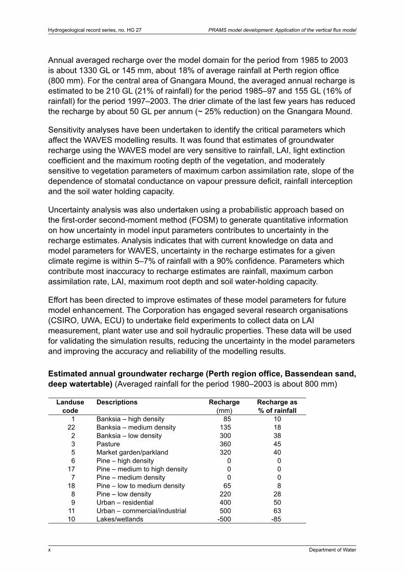
Analysis of simulation results indicates that the new VFM produces recharge estimates that are consistent with the previous estimates using other methods. The table reproduced at the end of this summary (Table 11 in text) shows the estimated annual rainfall recharge for various landuse classes under deep watertable (> 15 m, except the lakes/wetlands) using climate data for the Perth region office from 1980–2003 and for Bassendean soil. Recharge in the vegetated areas with Spearwood soil is 3–5% lower than in vegetated areas with Bassendean soil. This is because Spearwood soil has better soil water holding capacity and is capable of storing more winter rainfall for plant use late in summer when evaporative demand is high. Simulation results also indicate that recharge in the areas of Quindalup soil is similar to that in areas of Bassendean soil. For the Guildford soil, the major landuse is pasture. Recharge is about 10% of rainfall in the areas with deep watertable and becomes negative (discharge) in the area with shallow watertable.
x Department of Water
Hydrogeological record series, no. HG 27 PRAMS model development: Application of the vertical flux model
Annual averaged recharge over the model domain for the period from 1985 to 2003 is about 1330 GL or 145 mm, about 18% of average rainfall at Perth region office (800 mm). For the central area of Gnangara Mound, the averaged annual recharge is estimated to be 210 GL (21% of rainfall) for the period 1985–97 and 155 GL (16% of rainfall) for the period 1997–2003. The drier climate of the last few years has reduced the recharge by about 50 GL per annum (~ 25% reduction) on the Gnangara Mound.
Sensitivity analyses have been undertaken to identify the critical parameters which affect the WAVES modelling results. It was found that estimates of groundwater recharge using the WAVES model are very sensitive to rainfall, LAI, light extinction coefficient and the maximum rooting depth of the vegetation, and moderately sensitive to vegetation parameters of maximum carbon assimilation rate, slope of the dependence of stomatal conductance on vapour pressure deficit, rainfall interception and the soil water holding capacity.
Uncertainty analysis was also undertaken using a probabilistic approach based on the first-order second-moment method (FOSM) to generate quantitative information on how uncertainty in model input parameters contributes to uncertainty in the recharge estimates. Analysis indicates that with current knowledge on data and model parameters for WAVES, uncertainty in the recharge estimates for a given climate regime is within 5–7% of rainfall with a 90% confidence. Parameters which contribute most inaccuracy to recharge estimates are rainfall, maximum carbon assimilation rate, LAI, maximum root depth and soil water-holding capacity.
Effort has been directed to improve estimates of these model parameters for future model enhancement. The Corporation has engaged several research organisations (CSIRO, UWA, ECU) to undertake field experiments to collect data on LAI measurement, plant water use and soil hydraulic properties. These data will be used for validating the simulation results, reducing the uncertainty in the model parameters and improving the accuracy and reliability of the modelling results.
Estimated annual groundwater recharge (Perth region office, Bassendean sand, deep watertable) (Averaged rainfall for the period 1980–2003 is about 800 mm)
Landuse code
Descriptions Recharge (mm)
Recharge as % of rainfall
1 Banksia – high density 85 1022 Banksia – medium density 135 18
2 Banksia – low density 300 383 Pasture 360 455 Market garden/parkland 320 406 Pine – high density 0 0
17 Pine – medium to high density 0 07 Pine – medium density 0 0
18 Pine – low to medium density 65 88 Pine – low density 220 289 Urban – residential 400 50
11 Urban – commercial/industrial 500 6310 Lakes/wetlands -500 -85

Department of Water 1
PRAMS model development: Application of the vertical flux model Hydrogeological record series, no. HG 27
1 Introduction
The Water Corporation and Department of Water (formerly the Water and Rivers Commission — WRC) have jointly developed a groundwater model (Perth Regional Aquifer Modelling System, or PRAMS) for the Perth region (Figure 1) to assist with groundwater resource management and development of public water supply. PRAMS consists of three components: the Vertical Flux Model (VFM), a saturated model based on MODFLOW, and a GIS-based data management system (Figure 2). The VFM estimates the net recharge/discharge of water into/from the unconfined aquifer, whereas the MODFLOW-based saturated model determines the groundwater flows in the multi-layer aquifer system below the watertable. The two models have been developed in parallel and were tested separately before they were coupled. PRAMS version 3.0 is the most recently calibrated model, which fully integrates the VFM and the saturated groundwater model. The PRAMS model is supported by a GIS–based data management system that ensures the quality and integrity of the data used in the model.
The Water Corporation has been responsible for development of the VFM and its integration with the saturated model. Because of the complex nature of the project, the Corporation has engaged several research organisations and consultants to assist with the model development, including:
• Dr L. Townley of Townley & Associates Pty Ltd undertook the review of hydrological processes in the unsaturated zone in the Perth region with the aim of developing a conceptual VFM-based on the physical properties that control groundwater recharge in the region (Townley, 2000).
• Following a feasibility study to investigate the potential use of a biophysical recharge model (WAVES) as the modelling platform for the VFM, CSIRO has carried out the core work of the model development. This included development of the VFM manager and its integration to MODFLOW, field studies to measure soil hydraulic properties, vegetation density defined by leaf area index (LAI), and development of a methodology to derive LAI using Landsat image and ground truth data and model verification using data available. Field work is also currently being undertaken to collect data on the water balance for pine plantations on Gnangara Mound. This work has been described in detail in part 1 of the VFM report (Silberstein et al., 2004).
• Mr A. Allen, formerly of Department of Land Administration (DOLA) assisted in development of a methodology to derive historical landuse based on the Landsat data (Allen, 2003).
• A/Prof. K. Smettem of University of Western Australia (UWA) undertook lab analysis and in situ measurements of soil hydraulic properties (Smettem, 2002), and Mr M. Wells of Land Assessment Pty Ltd provided an overview of the soil

2 Department of Water
Hydrogeological record series, no. HG 27 PRAMS model development: Application of the vertical flux model
distribution in the Perth region based on the Agriculture WA (AgWA) soil database (Land Assessment Pty Ltd, 2001).
• Dr R. Froend of Edith Cowan University (ECU) investigated water use of native woodlands (Lam et al., 2004).
• Mr N. Milligan of CyMod applied the coupled model to both the pilot study area and the whole model domain (PRAMS 3.0) (CyMod, 2003, 2004).
A wide range of spatial and temporal data has been collected to support the model application (Canci, 2004). Whilst most of these physical data are not subject to change during model calibration and integration, some of the parameters derived from the data have undergone refinement and modifications in the pilot study and development of PRAMS 3.0 in order to minimise the modelling errors.
This report gives a brief overview of the model development process, describes issues which arose during application of the model, and modifications made to the VFM and datasets to address these issues. Final datasets implemented in PRAMS 3.0 are presented together with supporting information for the parameters used, particularly for the non-WAVES modules. This document also reports the estimated groundwater recharge under different climate, landuse, soil and watertable depth conditions, which reflect typical recharge rates for a range of representative recharge units (RRUs). Recharge analysis was undertaken to upscale the recharge estimates to regions of interest for a range of landuse and conditions. Simulated results from sensitivity analysis applied to the whole PRAMS model domain of some critical VFM parameters are described. Based on results of these analyses recommendations are made for further work that may improve the accuracy and reliability of the WAVES-based VFM.

Department of Water 3
PRAMS model development: Application of the vertical flux model Hydrogeological record series, no. HG 27
2 Development of a new vertical flux model (VFM)
2.1 Previous work on recharge estimates in the Perth region
2.1.1 Previous recharge estimates
Groundwater recharge estimates have been made at both local scale and regional scale on the Swan Coastal Plain using methods appropriate for semi-arid environments such as water balance, environmental tracing (chloride, bromide balance methods), isotopic analysis (tritium) and empirical relations based on other variables (such as rainfall). Empirical relations defining recharge as a percentage of precipitation generally are based on waterbalance studies, and have been widely used in the Perth region.
Bestow (1976) estimated that about 7.3% of the mean annual rainfall over the Gnangara area becomes groundwater recharge. Allen (1981) estimated that about 8.5% of rainfall recharges the aquifer in the northern area and 5.5% in the southern area. Davidson (1995) used flow net analysis and chloride balances to estimate the average recharge for the Perth metropolitan area and found that the recharge rate is about 15% of long-term averaged rainfall of about 870 mm. The PUWB model estimated that about 21% of the rainfall recharges the aquifer beneath urban Perth (Cargeeg et al., 1987).
Butcher (1979) undertook water balance analysis using soil moisture data measured by neutron probes and found that recharge under native woodland, young open and dense pine stands was 29%, 19% and 8% of rainfall respectively.
Farrington and Bartle (1991) used three methods (water balance, chloride balance, and rate of watertable rise) over a three-year period to estimate recharge under banksia and pines. They found 114 mm recharge under pines (15% of rainfall) and 173 mm recharge under banksia (22% of rainfall).
Sharma et al. (1991a,b; 1995) provide the broadest view of recharge under a range of landuse categories on the Gnangara Mound, although in many cases the results focus on gross recharge rather than net recharge (i.e. they do not account for phreatophytic withdrawals). Recharge was estimated by a combination of chloride and bromide methods, water balance methods, groundwater level fluctuations and mechanistic modelling.
For deep (> 15 m) watertable, it was found that recharge beneath mature pines was less than 4% of rainfall, recharge beneath banksia was 15% of rainfall and recharge beneath young pines was 32% of rainfall. With shallow depths to the watertable (5 to 7 m), Sharma et al. (1991a) found recharge of the order of 30% of rainfall for banksia, less than 16% for sparse pines and less than 8% for dense pines.

4 Department of Water
Hydrogeological record series, no. HG 27 PRAMS model development: Application of the vertical flux model
The average recharge beneath pasture near Lake Pinjar was estimated to be 50 to 60% of rainfall at sites with depths to the watertable of 4 m and 7 m, respectively (Sharma et al., 1991a).
Sharma et al. (1991b) studied the water balance at two farms practising irrigated horticulture between July 1989 and June 1991. Over the two-year period, irrigation accounted for 60 and 69% of the total water input to the two farms, the remainder being rainfall. Irrigation accounted for most of the input during summer. Of the total water input, 49% leached below the root zone at one farm, and 36% at the other. In other words, from 35 to 50% of the licensed irrigation withdrawal of 1500 mm/y was returned to the aquifer.
Recharge beneath urban lawns was studied between April 1992 and April 1994 (Sharma et al., 1995). Eight sites were equipped with lysimeters at a range of private gardens and sporting complexes. Depths to watertable varied from 3 m at three sites to 20 m at three others. Average depths of recharge in summer and winter on Bassendean sands were 263 and 602 mm, while corresponding two-year averages on Spearwood sands were 70 and 293 mm.
Thorpe (1985) used naturally occurring tritium as an indicator of groundwater recharge and found about 43% of rainfall recharges the aquifer on the top of the Gnangara Mound (site NR1) and 19% of rainfall at a site south of the mound (NR5). Appleyard (1995) used a similar method to estimate the recharge under urban areas in the Whitfords area and found that the net recharge is about 37% of average annual rainfall of 800 mm (by nature of the method used in his analysis, this recharge rate should be interpreted as the net results of rainfall recharge taking away the abstraction, e.g. domestic garden bores, which is approximately 10% of rainfall. Hence actual rainfall recharge should be about 10% higher than the value reported in his paper).
2.1.2 Previous VFM modelling studies
Recharge estimates by modelling vertical flux have also been made. The Perth Urban Water Balance (PUWB) model uses a spatially variable one-dimensional vertical flux model (VFM) that simulates the hydrological process in the unsaturated zone, and to calculate the net vertical flow of water to/from the saturated zone. The VFM implements an algebraic water-accounting model of vertical flow through the unsaturated zone. A simplified rule-based system having three layers, defined as the grass, tree and soil zones, is used. These zones reflect different evapotranspiration processes occurring at different depths within the unsaturated zone. Water, from rainfall recharge, moves vertically from one zone to another under gravity, based on an empirical algorithm that uses a set of rules relating antecedent moisture conditions to derive the net vertical flux to the superficial aquifer. In addition, a deep drainage algorithm was included to simulate the soil zone. This algorithm was an attempt to introduce a delayed response in vertical flux reaching the saturated zone.
Department of Water 5
PRAMS model development: Application of the vertical flux model Hydrogeological record series, no. HG 27
The VFM used in the PUWB model was developed based on a conceptual model that represents the recharge processes in urban settings. A recent review found that although the PUWB model represented the recharge adequately in urban areas, it does not give good estimates of recharge to the watertable (CyMod, 1999) in surrounding vegetated areas, which includes native banksia woodlands, pasture, market gardens and pine plantations.
2.2 New VFM development process
Deficiencies in existing recharge models for the Swan Coastal Plain led to the development of a new VFM model. A major criterion for the development of the new VFM was to incorporate the best available knowledge of the characterisation of the unsaturated zone in the Perth region, and an understanding of time-varying processes within the soil–water–landuse continuum, including processes of rainfall, interception, infiltration, evaporation, transpiration, soil storage, runoff and pumping (both domestic and institutional).
The development of this new VFM has been carried out in stages:
• Development of conceptual models (Townley, 2000)
• Feasibility study of the potential use of the biophysical recharge model WAVES (Hatton et al., 2001)
• Development of WAVES-based VFM and integration with MODFLOW (Barr et al., 2003; Silberstein et al., 2004)
• Data collection and verification of VFM using field data (Canci, 2004; Silberstein et al., 2004; Bekele and Silberstein, 2003; Hodgson, 2003; Xu, 2003)
• Pilot study to test the VFM - MODFLOW integration (CyMod, 2003)
• Full scale integration and calibration (CyMod, 2004)
The following sections give a summary of the outcome from these studies and details can be found in the individual reports.
2.3 Conceptual model of VFM for the Perth region
Recharge and discharge to and from the regional groundwater system is referred to as the ‘vertical flux’ in this study. The primary goal of the vertical flux model is to estimate this flux spatially across the model area as temporal input to the regional groundwater model. Consequently, the VFM must account for the various physical processes that act to determine the recharge and discharge from regional aquifers.
Recharge to the Perth groundwater system occurs principally from direct rainfall infiltration. Most of the rainfall occurs in the winter months leading to a strong

6 Department of Water
Hydrogeological record series, no. HG 27 PRAMS model development: Application of the vertical flux model
seasonal variation in the watertable, particularly where it is shallow. Small amounts of scheme water that are imported into urban or irrigated areas may also contribute to groundwater recharge through septic tank or grey water discharge, return flow in areas with over watering of gardens, and scheme losses due to leakage and maintenance.
2.3.1 Processes controlling groundwater recharge
Waterbalance processes that control groundwater recharge in the Perth region are well described in the Perth Urban Water Balance Study (Cargeeg et al., 1987) and in a recent review by Townley (2000). Figure 3 shows the schematic of recharge processes on the Gnangara Mound. Rainfall not intercepted by canopy, roofs and/or litter, infiltrates the soil across the air-soil interface or runs off. Some of the water that infiltrates the soil evaporates directly from the soil surface or is transpired by plants; some may be redistributed and stored in the soil profile and may percolate down. Redistribution is the continued movement of water (in all directions) through soil after water has stopped infiltrating at the ground surface. Percolation is defined as the downward flux of water in the unsaturated zone. Deep drainage is the percolation flux that moves below the depth where evapotranspiration no longer affects the downward movement of infiltrated water. The approximate depth at which deep drainage occurs is variable in both space and time, depending upon the soil properties and the maximum root depth of the vegetation grown on the surface. For most locations in the Perth region, deep drainage eventually becomes recharge, particularly on the Swan Coastal Plain, where the soil is dominated by permeable sands.
When deep drainage occurs, water continues to percolate through the unsaturated zone and, in most cases, reaches the regional watertable. At the watertable, water flux from the unsaturated zone to the saturated zone is defined as recharge. Deep drainage and recharge to the regional saturated zone are not necessarily equivalent at a given location and time because the infiltrating water may take some months or years to move through a thick unsaturated zone to the watertable. For the very thick unsaturated zones, particularly in the area between the Gingin and Darling Scarps, groundwater recharge may be transient due to the combination of climate variability and very long travel times of unsaturated flow.
Recharge is usually episodic for most locations in the Perth region, typically occurring during and after periods of high-volume winter rainfall when evapotranspiration is low. Groundwater levels on the Swan Coastal Plain show strong seasonal variation with peak or maximum water level occurring around October/November and minimum water level in April/May.
Recharge into the regional groundwater may be directly extracted by phreatophytic vegetation where the vegetation roots intercept the watertable (Froend et al., 1999).

Department of Water 7
PRAMS model development: Application of the vertical flux model Hydrogeological record series, no. HG 27
2.3.2 Water balance components for a conceptual model of vertical flux
Conceptual models of vertical flux provide a qualitative description of the processes controlling the spatial and temporal distribution of groundwater recharge. A primary component of the conceptual model of the VFM is the conservation of mass, or the water balance, which designates that the sum of all inputs, outputs, and storage changes in the system equals zero. Major components of the water balance in semi-arid environments such as the Perth region are rainfall, infiltration, runoff, evapotranspiration, redistribution, percolation and deep drainage (recharge).
2.3.2.1 Rainfall
Rainfall is the primary component of the water balance in Perth. The climate of the Perth region is Mediterranean with hot, dry summers and mild, wet winters. Approximately 90% of the rain falls between April and October. During the cool winter months, rain is produced from cold fronts associated with low-pressure systems whose centres pass from west to east through the region or just to the south and is usually accompanied by strong winds and cloudy skies. The hot, dry summers are caused by a belt of anticyclones. Occasionally, intense summer rainfall can occur from thunderstorms associated with a heat trough that forms along the west coast and drifts inland.
In addition to the strong seasonality of rainfall, recharge is also influenced by the spatial and temporal distribution, including its intensity and duration.
2.3.2.2 Evapotranspiration
Evapotranspiration is the second dominant component of the water balance in the Perth region. Evapotranspiration is the combined process of interception, evaporation and plant transpiration.
Interception occurs when roads, roofs or vegetation canopies catch rainfall and prevent its passage to the earth’s surface. The amount of interception depends on landuse, vegetation type, canopy cover and weather characteristics such as rainfall intensity and wind strength. Intercepted water is usually returned directly to the atmosphere by evaporation. However, in the Perth urban area, most of the interception occurs on impervious surfaces such as roads, parking lots and house roofs. In this case, intercepted rainfall may be redirected to subsurface sumps for infiltration, contributing significantly to groundwater recharge in urban areas.
Soil evaporation occurs when water that reaches the ground evaporates again directly from the soil surface or leaf litter. Its rate depends on atmospheric conditions (solar radiation, wind, temperature and humidity etc.) and on surface conditions (available litter and soil hydraulic properties).
Transpiration occurs when water is taken up through plant roots and travels through the interior of the plant to be lost to the atmosphere via evaporation through the

8 Department of Water
Hydrogeological record series, no. HG 27 PRAMS model development: Application of the vertical flux model
leaves. Transpiration depends on vegetation characteristics (species, root depth and density etc.), atmospheric conditions, and water availability within the soil (especially the distribution of soil moisture near the roots). Some plants, known as phreatophytes, have deep roots which intersect the watertable and are capable of withdrawing water directly from the watertable (Froend et al., 1999). Leaf area is believed to be a key factor that controls transpiration rates.
The general theory of evapotranspiration indicates that the availability of moisture, and the availability of energy for evapotranspiration and transport of water vapour away from the evaporating surface, are the most important controlling factors. In most areas of Perth (except for lakes and wetlands), the availability of moisture (rainfall) is less than the availability of energy for evapotranspiration and transport of water vapour for much of the time. However, groundwater recharge does take place over much of the Perth region. This is because the atmospheric demand and water availability are out of phase due to the Mediterranean climate and very low water holding capacity of the soils across the region. During winter, rainfall can exceed the water equivalent of the available energy for evapotranspiration, and part of the rainfall reaches the deeper soil layers beyond the reach of vegetation, resulting in recharge or storage of water in the soil.
Important physical parameters that control the processes of evapotranspiration include the incoming solar radiation, temperature, wind spread, available soil moisture, vegetation characteristics (species, root depth and density) and watertable depth. Vegetation density is measured by leaf area index (LAI), which is defined as the ratio of green leaf area to ground area under the tree canopy.
2.3.2.3 Infiltration, runoff and surface water
Surface runoff is generated either when the groundwater rises above the ground surface or the infiltration capacity of the unsaturated zone is exceeded by the rainfall input. The combination of a Mediterranean climate and highly permeable, sandy soils over much of the Perth region results in little direct surface runoff in most areas. Most rainfall infiltrates into the soil and is eventually returned to the atmosphere through evapotranspiration, or recharges the aquifer. The exception to this is in areas having low-permeable Guildford soil, where some runoff may occur during winter under high intensity rainfall conditions.
The amount of water that can infiltrate before runoff is generated depends on four factors: the rainfall intensity and duration (the rainfall intensity must be greater than the saturated hydraulic conductivity of the soil, and the rainfall duration must be greater than the time required for the soil to become saturated at the surface), infiltration capacity (how quickly the soil takes up water), the total storage capacity (how much water the soil can hold), and the antecedent conditions affecting the available storage capacity (how much water is being stored from previous storms).

Department of Water 9
PRAMS model development: Application of the vertical flux model Hydrogeological record series, no. HG 27
There are a few significant natural drainages or creeks within the study area, including the Moore, Swan and Canning Rivers, Gingin and Ellen Brooks. However, streamflows in most of the rivers are intermittent and occur predominantly as runoff over the catchments (most of which are outside the study domain) from rainfall. Sustained streamflow from discharging groundwater is limited to a few small brooks. A review of these river features indicates that most are acting to discharge groundwater (base flow) (Davidson, 1995). Consequently, infiltration from streamflow is not considered to be a significant component of groundwater recharge in the Perth region.
2.3.2.4 Redistribution/percolation, deep drainage and recharge
Redistribution, an unsaturated flow process governed by water-potential gradients and gravity drainage, is the continued movement of water through soil after infiltration has stopped at the ground surface. It is an important process that controls the amount of water percolating below the zone of evapotranspiration and becomes deep drainage. Redistribution occurs in response to both gravitational and capillary (matric) potentials, and includes upward flow in response to capillary suction, downward flow in response to both gravity drainage and capillary suction, and lateral flow in response to both capillary potential and heterogeneity in the soil. The initial redistribution of infiltration in wet soils generally occurs as gravity drainage. Gravity drainage can be relatively rapid when soils are fully saturated, but decreases significantly as the soil drains to a, subjectively defined, water content referred to as ‘field capacity’. Field capacity is the approximate water content at which the capillary potential holding water in the soil under suction is significant relative to gravitational potential, hence causing gravity drainage to be very slow. It is a conceptual term used to characterise the water holding capacity of a given soil. Field capacity is usually defined by the water content of the soil following a specified period of drainage (from full saturation) or when the drainage rate becomes negligible (Campbell, 1985). In general, the lower the permeability and the higher the field capacity for a given soil, the greater the potential that water infiltrating the soil will eventually be removed by evapotranspiration before it can percolate through the root zone to a depth where it becomes deep drainage.
Deep drainage will eventually become recharge to the watertable in most of the areas in the Perth region owing to the existence of permeable soil. There are, however, some areas between the Gingin and Darling Scarps where the watertable is very deep and unsaturated zones are very thick. The vertical permeability of the soil column may be very low, particularly where shale bands associated with Mesozoic sediments exist. In these areas, it is likely that perched watertables will develop and deep drainage becomes recharge to a perched saturated zone and may flow laterally to a local discharge area.
Redistribution/percolation and deep drainage in the unsaturated zone in most of the areas is assumed via the soil matrix and not via macropores and larger preferred pathways. The soils on the Swan Coastal Plain are typically unconsolidated
10 Department of Water
Hydrogeological record series, no. HG 27 PRAMS model development: Application of the vertical flux model
sands having very little clay and are highly permeable. Under these conditions it is unlikely that significant preferential flow will exist, as the unconsolidated sands are not prone to cracking or fissures and typically do not sustain preferential flow structures for any length of time. In addition, the inherent high hydraulic conductivity of the sands suggests that in areas where some preferential flow may occur, such as where long roots have created holes or soils are non-wetting (hydrophobic), its relative significance compared to matrix flow may be small. The exception to these conditions may occur in the Guildford soil, where preferential flow paths due to root voids, clay shrinkage and other mechanisms may allow significant preferential flow compared with that occurring via the matrix. However, the occurrence of Guildford soil is typically along the escarpment and in low-lying areas with shallow depth to watertable, where there is likely to be groundwater discharge rather than recharge.
Important factors controlling redistribution/percolation are the thickness of the unsaturated zone, soil layering, and hydraulic properties such as hydraulic conductivity (a measure of soil’s ability to transmit water) and its water retention characteristics (the ability of the soil to store and release water).
2.3.3 Effects of landuse on vertical flux
2.3.3.1 Effects of urbanisation
Urbanisation is characterised by the replacement of natural or rural vegetated landscape by a mottled combination of sealed impervious surfaces and grassed or other vegetated surfaces. Interception, transpiration, infiltration and percolation are substantially modified by the impervious surfaces in urban areas.
Buildings, roads, and other surface infrastructure such as drainage networks, and disposal facilities such as soakwells and infiltration basins, significantly change the flow pathways for precipitation to reach the watertable. In Perth, rainfall interception by roofs is commonly disposed on site via a soakwell at a depth of about one metre to comply with local government regulations. In addition, runoff from impervious surfaces such as roads and pavement is usually directed to a drainage system which normally directs the water to local infiltration basins. These infiltration basins may also be connected to larger drainage systems that discharge major storm water to rivers or the ocean. However, excess drainage usually occurs only in the areas with low-permeability soil or shallow watertable. As a result, urbanisation changes the recharge characteristics from diffused recharge with the slow infiltration and percolation under natural environments to concentrated point sources which migrate rapidly toward the watertable, particularly on highly permeable Spearwood or Bassendean sand.
Large amounts of water are also imported via the scheme supply and collected again in sewers or septic tanks. Additional recharge from the leakage of these distribution and collection networks and return flow in garden irrigation can also be substantial. Areas without connection to sewers also have additional recharge from septic tanks.

Department of Water 11
PRAMS model development: Application of the vertical flux model Hydrogeological record series, no. HG 27
The increase in recharge as discussed above may, however, be partially offset by increased use of domestic garden bores.
2.3.3.2 Effects of agriculture
Agriculture is characterised by the replacement of natural vegetation with some form of crop or pasture. Interception losses are changed and the transpiration requirements of the new vegetation may be substantially different. This in turn modifies the recharge to the watertable.
Irrigation of crops or pasture is often introduced in agricultural areas, usually using groundwater pumped on site. Most of the irrigated water is used by plants to meet the evaporative demand, both for transpiration and to simply maintain temperature control. However, research has showed that a proportion of the irrigation water may return to recharge the aquifer (Sharma et al., 1991b).
2.3.4 Conceptual model for the vertical flux model
Unsaturated flow in the Perth region is characterised by cyclic fluctuations in soil moisture as water is replenished by rainfall and removed by evapotranspiration and recharge to the watertable. Infiltration may cause a rise in the watertable, whereas upward capillary flow from the watertable may occur in areas with shallow watertable and high evapotranspiration rates. Unsaturated flow is primarily vertical since gravity plays a major role during infiltration and permeable soils exist over most of the study area. Figure 4 shows a schematic of vertical flux under a natural environment.
The conceptual model of water balance processes and vertical flux in the Perth region is based on the law of conservation of mass: any change in the water content of a given soil column during a specified period must be equal to the difference between the amount of water added to the soil column and the amount of water withdrawn from it. Conceptually, the vertical flux over the period of interest can be expressed as:
R = P − EVT − RO − ∆S (1)
and
EVT = I + E + T (2)
where R is deep drainage (recharge); P is rainfall; EVT is evapotranspiration (which consists of interception loss, I, litter interception and soil evaporation, E, and transpiration, T); ΔS is the change in soil water storage; and RO is surface runoff.
The water balance equation often can be simplified by assuming one or more of the terms to be negligible. For example, runoff is not an important water balance process in most of the study area. Routing of surface water flow can be ignored and any infiltration excess can be removed from the system, based on order of magnitude arguments. This removes the need for a detailed surface water model for this study.

12 Department of Water
Hydrogeological record series, no. HG 27 PRAMS model development: Application of the vertical flux model
Similarly in the urban areas where the recharge is dominated by point sources such as soakwells and infiltration basins, changes in soil storage have relatively small impact on recharge. This allows a simplified recharge model to be used in the urban environment.
2.3.5 Characterisation of data for the conceptual VFM
As described in the previous sections, critical attributes of the vertical flux as represented by equations (1) and (2) are climate, landuse and vegetation characteristics (species, roots, LAI), soil hydraulic properties and watertable depth. There is considerable spatial and temporal variability in the key attributes across the model domain (e.g. Figure 5 for spatial variations of climate and landuse) that must be incorporated in implementation of the conceptual model.
2.3.5.1 Climate
Two important climatic variables affecting the vertical flux in equation (1) are the rainfall (P) and the available energy, the major driving force for evapotranspiration (EVT).
The average annual rainfall ranges from about 450 mm in the northeast to about 1200 mm in the southeast of the study area (Figure 5). The average annual pan evaporation increases from 1600 mm in the south to about 2200 mm in the north. To account for the spatial variation in climatic conditions, five climatic zones based on climatic indices derived from monthly rainfall, pan evaporation and temperature data (Aryal and Bates, 2001) have been defined (Figure 6). The variation in climatic characteristics within each zone are considered to be relatively small and climate data (rainfall, solar radiation, temperature and vapour pressure deficit) from a representative climate station within the area has been used to drive the recharge modelling. The duration and intensity of rainfall and their effects on the infiltration and runoff are accounted for explicitly by allowing the VFM to run any specified interval within a general daily time step.
2.3.5.2 Landuse and vegetation density (LAI)
Landuse in the modelling area is complex and varies both in space and time. Recharge mechanisms are significantly different under urban areas and the vegetated area. In urban areas, groundwater recharge is dominated by point sources through soakwells and sumps on individual properties and larger storm infiltration basins that collect the runoff from impervious surfaces such as roofs and roads. Under vegetated areas, recharge varies considerably dependent upon vegetation characteristics (species, root depth and density (LAI)). Shallow-rooted vegetation such as pasture uses much less water than deep-rooted trees. Alternatively, dense vegetation such as forests of pines (plantations) and dense understorey can intercept and transpire much more water than grass and open native woodlands. Previous studies have shown a wide range of recharge rates in the region, from negligible recharge under pine plantations up to 60% of rainfall under pasture.
Department of Water 13
PRAMS model development: Application of the vertical flux model Hydrogeological record series, no. HG 27
To account for the recharge variation under different landuses and vegetation types, landuse within the study area is first classified into a number of primary categories:
• native woodlands
• pine plantations
• dryland cropping/pasture
• irrigated horticulture (market garden), parklands and golf courses
• urban
• lakes and wetlands.
The composition of these primary classifications for the study area for year 2002 is shown in Figure 7.
For the native woodlands and pines, EVT is a strong function of leaf area index. LAI not only affects the rate of transpiration but also controls the proportion of radiation reaching the soil surface, which in turn influences evaporation rates from that soil surface. To account for the difference in tree EVT under different densities, the native woodlands are further subdivided into low-, medium- and high-density classes. Similarly, the pine plantations are delineated into five subclasses: high, medium to high, medium, low to medium, and low density. Both native and pine plantations are characterised by the density of trees as measured by LAI, which is derived from ground truth data and Landsat imagery (Hodgson, 2003). In the urban area, further subdivision is made to distinguish commercial areas, which have relatively high recharge rates, from the residential areas.
There are thirteen classes of landuse for the whole model domain. Figure 8 shows the landuse classification map for 2002.
Changes in landuses have occurred due to urbanisation, burning, or clearing for pine plantations. Changes in rainfall recharge can be substantial, from 0 to 60%. An important part of the modelling objective is to account for spatial and temporal changes, hence the VFM needs to accommodate landuse changes. For this study, the spatial distribution and temporal changes of these landuse classifications have been determined at two-yearly intervals from satellite imagery, air photographs and other cadastral and mapping information (Canci, 2004).
2.3.5.3 Soil lithology and hydraulic properties
The soil column regulates the rate of infiltration, stores and redistributes the infiltrated water, and controls the supply of water for plant uptake and evaporation at the soil surface. Owing to the Mediterranean climate of the Perth region, there is very little rainfall during the summer months when evaporative demand is highest. Under these conditions transpiration by vegetation is constrained by the available soil moisture carried over from winter rainfall, unless the vegetation is able to access groundwater. The major soil properties affecting these processes are hydraulic conductivity (a

14 Department of Water
Hydrogeological record series, no. HG 27 PRAMS model development: Application of the vertical flux model
measure of soil’s ability to transmit water) and its water retention characteristics (the ability of the soil to store and release water).
The soil in most of the model domain is characterised by coastal sand with high permeability, very low water holding capacity, very low organic content and little or no clay. Soils with higher clay or organic content occur along the eastern margin associated with swamps and wetlands and in areas of the Dandaragan Plateau (McArthur and Bettenay, 1960). To account for the spatial variability in hydraulic properties of the soil, six different soil profiles were identified based on the soil pattern, geomorphology and surface geology. These six types are the Quindalup, Spearwood, Bassendean, Guildford, Mesozoic and Lacustrine soil profiles. The spatial distribution of these soil profile types is shown in (Figure 9). Changes in the soil hydraulic properties with depth are incorporated in the definitions of soil layers for each profile, which are based on lithological logs of drilling holes and soil maps provided by AgWA. Tables 1 and 2 show the conceptualisation of soil type and layers. For Spearwood and Bassendean soil profiles, two topsoil layers and one subsoil layer were used, but for the remainder only two soil layers (topsoil and subsoil) were defined. Hydraulic properties (unsaturated hydraulic conductivity K(Ψ) and water retention K(ψ)) for each soil type were derived based on data from in situ field measurements (Smettem, 2002) and laboratory analysis (Salama et al., 1999; Vermooten, 2002; Smettem, 2002) wherever possible (Xu, 2003).
2.3.5.4 Depth to watertable
A watertable close to the surface may enhance soil evaporation because of increased soil water supply from the watertable through the capillary fringe. In areas where vegetation intersects the watertable, groundwater may be withdrawn directly from the capillary fringe by vegetation (Froend et al., 1999), thereby increasing the transpiration rate and reducing the net groundwater recharge.
Depth to the watertable at a particular site is determined as the difference between the surface elevation and the level of the watertable. The watertable, however, changes spatially and temporally with a very strong seasonal variation in response to the climate and abstraction in some areas. To facilitate accurate determination of depth to watertable, high-resolution digital elevation models (DEMs) with a vertical accuracy of ± 2.0 m were used to define the surface elevation across the model domain. The groundwater levels generated by the saturated groundwater model are used as the watertable at a particular site and time. To incorporate the effects of change in the groundwater level, the VFM is designed to be dynamically coupled to the saturated groundwater model.

Department of Water 15
PRAMS model development: Application of the vertical flux model Hydrogeological record series, no. HG 27
Table 1 Soil profile classification and lithology associated with geomorphology and surface geology
Soil profile
Lithology Geomorphic element Major soil groups Surface geology
Quindalup Eolian and littoral calcarenite
Quindalup Dune system Calcareous deep sand Yellow/brown shallow sand Calcareous shallow sand Yellow deep sand
Safety Bay Sand
Spearwood Coarse-medium grained eolian calcarenite and yellow sand
Spearwood Dune system Yellow deep sand Pale deep sand Yellow/brown shallow sand
Tamala Limestone
Bassendean Leached, siliceous, eolian grey sand
Bassendean Dune system Pale deep sand Semi-wet soil
Bassendean Sand
Guildford Fluvial interbedded sand, clay and conglomerate, calcareous in places Lateritic
Pinjarra Plain Ridge Hill Shelf
Yellow deep sand Pale deep sand Duplex sand gravel Grey deep sand duplex Wet, semi-wet soil
Guildford Formation Ridge Hill Sandstone Yoganup Formation
Mesozoic Laterite, sand, sandy clay
Dandaragan Plateau Pale, red, yellow deep sand Duplex sandy gravel Grey deep sand duplex
Mesozoic Formations
Lacustrine Clay and peat Modern and ancient wetlands, interdunal corridors and swales.
Wet and semi-wet soil Quaternary alluvium and lacustrine deposits within Tamala Limestone and Bassendean Sand
Table 2 Layers and soil characteristics of typical soil profiles
Soil profile No. of layers
Thickness of soil layers Brief description
Quindalup 2 1: topsoil A, 0.5 m Calcareous sand with some organic material, high permeability, low water holding capacity
2: subsoil B, up to 50 m Calcareous sand, high permeability, very low water holding capacitySpearwood 3 1: topsoil A, 0.15 m Calcareous sand with some organic material, high permeability,
relatively better water holding capacity.2: topsoil B, 0.35 m Calcareous sand, very high permeability, low water holding capacity3: subsoil C, up to 50 m As above
Bassendean 3 1: topsoil A, 0.15 m Quartz sand, some organic material, high permeability, slightly better water holding capacity.
2: topsoil B, 0.35 m Quartz sand, high permeability, low water holding capacity.3: subsoil C, up to 50 m Quartz sand, very high permeability, very low water holding capacity.
Guildford 2 1: topsoil A, 0.5 m Clay and sandy clay, low permeability2: subsoil B, up to 30 m As above
Mesozoic 2 1: topsoil A, 4 m Laterite/sand, high permeability2: subsoil B, up to 30 m Sand, sandy clay, moderate to high permeability
Lacustrine 2 1: topsoil A, 2 m Clay and peat, very low permeability2: subsoil B, up to 30 m Fine-medium grain sand, high permeability on coastal sand dunes

16 Department of Water
Hydrogeological record series, no. HG 27 PRAMS model development: Application of the vertical flux model
2.4 Modelling of vertical flux
2.4.1 Methodology
Vertical flux models estimate the spatial and temporal distribution of recharge over the study area by approximating the water balance processes given in equations (1) and (2) using the key attributes that control the vertical flux.
Currently, a variety of approaches with different levels of complexity is being employed to model the governing processes to simulate vertical fluxes in the unsaturated zones and determine groundwater recharge (Scanlon et al., 2002). These approaches can be broadly categorised into two groups: soil water storage routing approaches (bucket model) and process-based models. The bucket model considers the soil storage as a reservoir (or a series of connected reservoirs) containing water, which is balanced in each time step. The process-based model describes the soil water movement based on Richards’ equation and incorporates more detail of the climate–soil–water–vegetation interactions.
A previous model of the Swan Coastal Plain, namely, the Perth Urban Water Balance (PUWB) model, used a bucket model that simulates spatially variable one-dimensional vertical flow to calculate the net vertical flow of water to/from the saturated zone (Cargeeg et al., 1987). The PUWB VFM implements an algebraic water-accounting model of vertical flow through the unsaturated zone, using simplified rule-based algorithms. Whilst the PUWB model represents the recharge adequately in urban areas, it was found that it did not give good estimates of recharge in the vegetated areas (CyMod, 1999).
Current and future groundwater resource development is highly constrained by the response of ecosystems in areas of native vegetation. Modelling tools that are designed to explore the sensitivity of the region to future abstraction, climate and landuse change must therefore be able to characterise the complex interactions between the soil, vegetation and rainfall. One of the criteria for developing a new model was to replace essentially empirical models, such as PUWB, with a physical-based model for those processes that are spatially and temporally dominant.
Given that over 90% of the area in the modelling domain is covered by natural vegetation, pine plantations and pasture/cropping, use of a process-based model was considered to be the best option to estimate recharge, taking into account the variation in vegetation, climate, depth to watertable and soil properties.
For other landuse classes, the use of the process-based model is inappropriate or unnecessary. This may be because the watertable is above, ‘or close to’, the ground surface (e.g. lakes and wetlands) or because anthropogenic factors govern the recharge (e.g. market gardens, urban areas). The VFM provides alternative, and more computationally efficient, algebraic models based on rainfall and pan evaporation to calculate net recharge due to rainfall for those areas. Recharge
Department of Water 17
PRAMS model development: Application of the vertical flux model Hydrogeological record series, no. HG 27
by return flow of irrigated water is handled separately in the saturated model by adjusting the abstraction from the superficial aquifer.
Assessment of the process-based models applicable to the environments of the Perth region, and review of the modelling requirements of the Water Corporation and Department of Water, have led to the use of the biophysical model WAVES, developed by CSIRO (Zhang and Dawes, 1998) as the modelling platform for the new VFM to calculate recharge under pasture, pine plantations, and native woodlands. WAVES emphasises the physical aspects of soil water fluxes and the physiological control of water loss through transpiration. The model can also be used to simulate the hydrological and ecological effects of vegetation management options (e.g. for recharge enhancement), or the water balance implications of changed climatic conditions.
Process-based models such as WAVES are usually computationally intensive and it is impractical to run a process-based model for each node of the saturated flow model (i.e. for more than 25 000 nodes) over the modelling domain, which covers more than 6000 km2. To overcome the computational issues and to adequately address the spatial variability of the key parameters that dominate the recharge processes, a new methodology based on the concept of representative recharge units (RRU) was developed (Silberstein et al., 2004).
A review of the physical inputs to the various components of the vertical flux model indicates that there are significant yet limited numbers of combinations of parameters that hold over the Swan Coastal Plain. The clustering of important model parameters provides an opportunity to reduce the computational requirement by only solving the soil distribution at unique nodes and using the solution at all other nodes that are a member of that group of variables.
The approach first classifies the modelling domain into a number of designated RRUs, which are based on climate, landuse (including vegetation characteristics), soil profile and watertable depth. It is assumed that hydrological properties are homogeneous within each RRU; and that all cells that share the same RRU will have similar recharge characteristics, and will have a similar soil moisture distribution and net recharge. Simulations are then carried out for each RRU to estimate the recharge using the WAVES model or an algebraic model, depending upon the landuse. Recharge for each cell in the modelling domain is determined using the VFM simulation results and watertable depth provided by the saturated groundwater model.
2.4.2 VFM recharge models
2.4.2.1 WAVES model
A full description of the WAVES model can be found in a report by Zhang and Dawes (1998). WAVES is a one-dimensional, daily time-step model that simulates the fluxes of water and energy between the atmosphere, vegetation, and soil systems. It is a

18 Department of Water
Hydrogeological record series, no. HG 27 PRAMS model development: Application of the vertical flux model
process-based model that couples these systems by modelling the interaction and feedback between them.
WAVES models the following processes on a daily time step:
• interception of rainfall and light by canopy
• surface energy balance
• carbon balance and plant growth
• soil evaporation and canopy evapotranspiration
• surface runoff and infiltration,
• saturated/unsaturated soil moisture dynamics (soil water content with depth)
• drainage (recharge)
• solute transport of salt (NaCl)
• watertable interactions.
A diagram of the components of WAVES is shown in Figure 10. The model is based on five balances:
• Energy balance: partitions available energy into canopy and soil for plant growth and evapotranspiration (Beer’s law)
• Water balance: handles infiltration, runoff, evapotranspiration (Penman-Monteith equation), soil moisture redistribution (Richards’ equation), drainage, and watertable interactions;
• Carbon balance: calculates carbon assimilation using integrated rate methodology (IRM) and dynamically allocates carbon to leaves, stems, and roots, and estimates canopy resistance for plant transpiration
• Solute balance: estimates conservative solute transport within the soil column and the impact of salinity on plants (osmotic effect only)
• Balance of complexity, usefulness, and accuracy.
The energy balance module calculates net radiation from incoming solar radiation, air temperature, and humidity, then partitions it into canopy- and soil-available energy using Beer’s law. Evapotranspiration is calculated using the Penman-Monteith equation with available energy, vapour pressure deficit, and air temperature as inputs. The Penman-Monteith equation is a ‘big leaf’ model based on the combination of energy balance and aerodynamic principles. It requires estimation of aerodynamic and canopy resistances. The aerodynamic resistance of the plant canopy is currently estimated by a constant value, whereas canopy resistance is calculated as a function of net assimilation rate, vapour pressure deficit, and CO2 concentration. WAVES couples canopy and atmosphere using the ‘omega approach’ proposed by Jarvis and McNaughton (1986) and handles the multi-layer canopy explicitly.

Department of Water 19
PRAMS model development: Application of the vertical flux model Hydrogeological record series, no. HG 27
The soil water balance module handles rainfall infiltration, overland flow, soil and plant water extraction, moisture redistribution, drainage (recharge), and watertable interactions. Soil water movement in both the unsaturated and saturated zones is simulated using a fully implicit finite-difference numerical solution of a mixed-form of Richards’ equation. Overland flow can be generated from the rainfall rate exceeding the infiltration rate of the soil, and when rain falls on a saturated surface.
WAVES accounts for antecedent moisture conditions in the root zone and deep unsaturated zone, for different plant species, extent of plant development, root zone depth, and the physical characteristics of soil type (soil moisture characteristic). This model has been shown to simulate water dynamics and vegetation growth correctly for a wide variety and combinations of climate, soil and vegetation type (Zhang et al., 1996; 1999).
Assumptions under which the WAVES model was developed are discussed in the report by Zhang and Dawes (1998).
2.4.2.2 Verification of WAVES
To demonstrate the applicability of WAVES to conditions existing on the Swan Coastal Plain, the model has been applied to several datasets to compare the simulation results with recharge derived from field measurements, including:
• water level data collected by CSIRO for the winter of 1998 (Hatton et al., 2001)
• data from neutron moisture meter access tubes installed at Pinjar (PM6, PV3)
• datasets collected by DEC in a field experiment in the McLarty plantation at Myalup, northeast of Harvey, to investigate the growth and water use of Pinus pinaster under different stand densities and fertiliser applications.
The comparison shows a reasonable agreement given the uncertainties in the site characterisation (soil, LAI etc. see Part 1 of the report by Silberstein et al., 2004). In particular, application of WAVES to the McLarty datasets has shown that the model (with vegetation growth module active) can reproduce the leaf area dynamics, wetting front infiltration and the seasonal soil water storage cycle (Bekele and Silberstein, 2003). This gives some confidence in using WAVES as the recharge modelling engine for PRAMS.
2.4.3 Algebraic models
Under certain conditions, some processes or components of the VFM described in equations (1)-(2) are amenable to simplification; typically those where the dominated flux bypasses the soil column, such as soakwells/infiltration basins connected to the soil below the root zone, point source recharge/discharge, and direct evaporation from a free surface or areas with no vegetation. For these landuse classes (urban, lakes/wetland and parkland/market garden), a process-based model is not required as the storage of water in the soil column has insignificant impacts on the vertical
20 Department of Water
Hydrogeological record series, no. HG 27 PRAMS model development: Application of the vertical flux model
flux reaching the watertable. The RRUs that have these characteristics are simulated using algebraic models with one to three parameters.
The algebraic models have a general form
R = α × P − β × PE (3)
where R = net recharge, P = rainfall, PE = pan evaporation, coefficients α and β can be constant (LINEAR model) or varying with watertable (PIECEWISE_LINEAR model); see Barr et al. (2003) for details.
The parameter coefficients for rainfall and pan evaporation for the non-WAVES recharge model were estimated based on available daily data but were subject to refinement as part of the calibration of the coupled model (CyMod, 2004). Initial estimates of these parameters are given in Table 3 and discussed below.
2.4.3.1 Urban
Recharge in the Perth urban area is dominated by point sources generated from soakwells and infiltration basins which manage runoff from roofs and other impervious surfaces. Leakage from distribution and collection networks and return flow in garden irrigation can also generate substantial recharge. This increase in recharge may be partially offset by increased use of domestic garden bores. An alternative approach for urban recharge is to estimate or quantify individual components. The Perth Urban Water Balance model used this methodology with some success (Cargeeg et al., 1987). However, such an approach requires a large amount of data, most of which is spatially variable and highly uncertain, and is likely to lead to a large uncertainty in the final estimate (Lerner, 2002).
PRAMS takes a holistic approach to dealing with recharge in the urban area. The abstraction of domestic garden bores is treated in the saturated model as distributed negative recharge and return flow is accounted for by discounting the abstraction rate. Other recharge in the urban area is calculated using the LINEAR model in the VFM. The effects of reticulation recycling, and the collection and disposal of runoff from impervious surfaces are simplified by specifying an equivalent recharge coefficient as a percentage of rainfall that is directed into the unsaturated zone below the root zone. Use of a recharge coefficient allows a simple model specifying direct recharge to the aquifer to be used. Elimination of storage in the unsaturated zone is acceptable because of the typically high hydraulic conductivity and low water holding capacity of the Bassendean and Spearwood sands in most areas of urbanisation. The point source nature of much of the infiltration results in the rapid vertical migration of recharge to the saturated zone.
Recharge by return flow of irrigation water from domestic garden bores is handled separately in the saturated model by adjusting the abstraction from the superficial aquifer. A recent study (Aquaterra, 2001) indicates that about 30% of all households in Perth have garden bores and abstract a total of more than 110 GL per annum. It

Department of Water 21
PRAMS model development: Application of the vertical flux model Hydrogeological record series, no. HG 27
is estimated that about 20–30% of irrigation water will recharge the aquifer as return flow (Davidson and Yu, 2004). PRAMS assumes a return flow of 30% of irrigation water.
Urban landuse is further classified into residential and commercial/industrial areas to account for the variations in recharge. The coefficients of the LINEAR models were initially estimated empirically from data such as the impervious surface (roof and pavement) area and minor adjustments were made as a part of PRAMS 3.0 calibration (CyMod, 2004).
Residential: PUWB studies undertook detailed investigation into the percentages of roofed and paved areas in a typical suburb. It was found that for the low-, medium- and high-density areas, the percentages of roofed are 8.8%, 18.0% and 37.0% and the percentages of paved are 8.4%, 13.2%, 15.4% respectively. Analysis of data for the PUWB model for the area north of the Swan River indicates that for the metropolitan area, the averaged percentages of roofed and paved are about 20% and 15% respectively. About 80–90% of rainfall falling on roofs will reach the groundwater via soak wells and 60–70% of rainfall on the paved areas will be collected and infiltrated in infiltration basins (Prince, 1997). For lawns and gardens, net rainfall recharge rate is estimated as 30–40% of annual rainfall. This indicates that rainfall recharge alone is in the range of 45–55% of rainfall in residential areas.
Loss from the water distribution networks in Perth is estimated to be around 10% of total supply, which may result in an additional recharge to the superficial aquifer of as much as 20 GL/a. A recent Domestic Water Use Study shows that about 54% of household water use is for backyard garden irrigation (Loh, M., 2004, pers. comm.). Assuming that 20% of the irrigated water becomes return flow to the aquifer, this could represent another 20 GL/a of recharge in the urban area. Thus leakage and return flow may contribute about 3–4% of rainfall to groundwater recharge. Areas without connection to sewers also have additional recharge from the discharge of septic tanks. However, these areas are gradually reducing owing to implementation of the sewerage infill program.
The combined recharge in residential areas with sandy soils and depth to watertable of more than 10 m is estimated to be between 48 and 60% of rainfall.
Commercial/Industrial: Analysis similar to that above indicates that the average percentages of roofed and paved surfaces for the commercial and industrial areas are about 40% and 35% respectively. This gives a recharge rate of 60–70% of rainfall in these areas.
In areas with soils of low permeability and shallow watertable, part of the estimated recharge will become drainage instead of groundwater recharge. PRAMS 3.0 uses the Drain Package in MODFLOW to handle drainage. Both natural drainage and the major man-made drainages operated by the local councils and the Water Corporation have been incorporated in the PRAMS 3.0 model.

22 Department of Water
Hydrogeological record series, no. HG 27 PRAMS model development: Application of the vertical flux model
2.4.3.2 Market garden/parkland
It was originally proposed to use separate landuse classes for market gardens (horticulture) and parkland, since irrigation of market gardens is much more intensive than that in parkland. However, it is difficult to distinguish these two landuses using Landsat data. As a result, the two classifications were amalgamated into one market garden/parkland landuse class. The classification includes parklands, golf courses, and market gardens and other irrigated crops.
These areas are subject to manipulation by human activity. Typically, groundwater is used to provide water for plants, in addition to that provided by rainfall. To simplify the recharge calculation, the net recharge is split into two parts: recharge due to rainfall, and return flow from irrigation. Recharge from rainfall is modelled via a recharge coefficient as percentage of rainfall using the LINEAR model in the VFM, whilst return flow from irrigation is accounted for by discounting the abstraction rates in the relevant area.
The water used for irrigation is typically abstracted from the superficial aquifer by bores in close proximity to the area that is to be irrigated. Research on the water used by market gardens, and other irrigators, suggests up to 50% of applied water may recycle back to the watertable (Sharma et al., 1991b). However, recycling is a function of how much water in excess of plant requirements is applied. The DoW issues licences for irrigation based on optimised plant water requirements. Consequently, in the absence of over pumping, the irrigation of market gardens and other areas should not result in significant recycling. Davidson (1995) estimated that recycling may be closer to 20%. PRAMS 3.0 discounts all private licensed abstraction from the superficial aquifer by 20%.
Rainfall recharge from market gardens is expected to be high because roots of the plants in these areas are commonly shallow and the evaporative demand is low and constrained by the available solar energy in winter. Field investigations by CSIRO (Salama et al., 1999) using lysimeters in a strawberry farm on the Gnangara Mound showed that recharge rates during the winter period of 1998 amounted to 75% of the rainfall (421 mm out of 558 mm of rainfall), whereas Sharma et al. (1991b) estimated that return flow is 40% of applied water. The VFM takes a conservative approach for calculation of recharge in these areas and uses a coefficient of 0.4 for α for net rainfall recharge calculation.
2.4.3.3 Lakes and wetlands
There are many lakes and wetlands on the Swan Coastal Plain that are permanently or seasonally inundated or waterlogged. The majority of these lakes are ‘flow through’ lakes (Townley et al., 1993) where the heads of the watertable and levels of the lakes are coincident. The existence of a lake is defined by topography and no special mechanisms other than evaporation are required to model lakes. Hence we use a simpler modelling approach based on the difference between rainfall and evaporation

Department of Water 23
PRAMS model development: Application of the vertical flux model Hydrogeological record series, no. HG 27
from a water body. The VFM uses the PIECEWISE_LINEAR model to simulate the recharge/discharge in the wetlands (Barr et al., 2003). The saturated flow model will account for inflow to, and outflow from, the lakes/wetlands.
The Department of Water (formally WRC) has mapped the distribution of lakes/wetlands on the Swan Coastal Plain (Hill et al., 1996). However, owing to lower than average rainfalls, increasing groundwater abstraction and maturing pine plantations, groundwater levels in the region have been declining over the past two decades. Water levels in many areas that were classified as wetlands/lakes have dropped and hydrological processes in these areas are now dominated by plant water use and hence are better modelled by WAVES. In this study, only areas that appeared as a body of water when the satellite images were taken (usually in December or January) were classified as lakes/wetlands. In order to accommodate the areas which are seasonally inundated, the VFM implements a strategy that forces any landuse type to automatically become a lake/wetland if the watertable depth at a particular cell is less than a value specified in the definition file. This value is currently set at 5 cm.
The lakes/wetlands landuse as classified above is essentially an evaporative basin. The VFM uses a coefficient of 1.1 for rainfall to account for additional inflows from the surrounding area. Evaporation from the water surface is assumed to be 0.8–0.85 of pan evaporation and reduces linearly to zero when the groundwater level falls 3 m below the ground surface. The evaporation coefficient is based on the values recommended by AgWA for the Perth region (Luke et al., 1987).
Table 3 Recommended parameters for simple recharge models
Landuse Model α β EVT extinction depth (m)
Urban: residential LINEAR 0.48–0.6 0 n/a
Urban: commercial LINEAR 0.6–0.7 0 n/a
Wetland/lake PIECEWISE-LINEAR 1.1 0.8–0.85 3.0
Parkland/market garden LINEAR 0.4 0 n/a
2.5 Data requirements for VFM
Data inputs for the VFM include:
• gridded maps that show spatially distributed landuse, including vegetation classification and leaf area index, climate domain, soil classification and a table of watertable depths at which simulations will be carried out
• temporal landuse maps currently at two-year intervals
• daily climate data for each climate domain, consisting of rainfall, pan evaporation, solar radiation, maximum and minimum temperature and vapour deficit

24 Department of Water
Hydrogeological record series, no. HG 27 PRAMS model development: Application of the vertical flux model
• soil data, details of soil layers in the soil profile and soil hydraulic properties for each soil layer. The hydraulic properties required as inputs in the form of soil tables for WAVES include the soil water retention curves and the unsaturated hydraulic conductivity characteristic curve
• the vegetation water use parameters and the root distributions with depth for native woodland, pines and pasture.
Full details of datafiles required for PRAMS 3.0 are given in Appendix I.
2.6 VFM manager and integration with MODFLOW
A program (VFM manager) has been developed to manage the data flow to the VFM models and integrate with the MODFLOW model (MODFLOW 96 and 2000).
Major tasks for the VFM manager include:
• to classify the RRUs for the whole model domain climate, landuse, soil profile and watertable depths at which simulations will be carried out
• to select the recharge model to run for individual RRUs
• to manage data input to the recharge models
• to run the recharge models and accumulate results for each stress period
• to pass the calculated recharge/discharge back to MODFLOW for each cell.
A full description of the VFM manager can be found in Barr et al. (2003).
2.7 Pilot study and full-scale implementation
A pilot study was undertaken on a subregion of the whole PRAMS modelling domain to evaluate the coupled model and provide a quantitative understanding of the linkage between the VFM and MODFLOW. This also provided information on the relationships between the aquifer response and recharge from different landuses. Initially, the one-layer saturated groundwater model developed by URS (2001) for the superficial aquifer in the South Gnangara Mound was used for the pilot study. However, analysis of the model parameters revealed that the spatial distribution of hydraulic conductivity in this model is significantly different from the conceptual hydrogeology described by Davidson (1995) and used in PRAMS 2.1. Simultaneously, the Corporation engaged CyMod to develop a local model to assist with the operation of the Lexia borefield (CyMod, 2003). The model then became available and was used for the pilot study.
The pilot model covers an area of about 1050 km2 from the Swan River in the south to the Lake Pinjar in the north (Figure 1). A uniform grid of 200 by 200 m is used with three vertical layers representing the superficial and Mirrabooka aquifers. The pilot study area is representative of the VFM landuse classes in the full domain, and
Department of Water 25
PRAMS model development: Application of the vertical flux model Hydrogeological record series, no. HG 27
part of the area has shallow watertable. This allows the pilot model to be used as a comprehensive test of dynamic linkage between the VFM and MODFLOW under these conditions.
Calibration of the pilot model was initially undertaken by accepting the recharge rate calculated by the VFM and adjusting, within the constraints of the conceptual hydrogeology, the horizontal and vertical hydraulic conductivity in the saturated model to match the measured water levels at calibration bores. It became apparent that the model could not be adequately calibrated using this approach. Most of the issues identified by this process were related to data specification but some were caused by the implementation of WAVES in the VFM. The significance of some of the issues was apparent only when the coupled model was applied to the full model domain, and hence the pilot study and full-scale implementation were overlapped in an iterative process. The main issues and measures adopted to address these are discussed below.
2.7.1 Excessive water uptake for shallow watertable under dense pines
Preliminary calibration of the pilot model indicated that the model performance in areas with deep watertable was good. In areas with shallow watertable, the WAVES model over predicted water uptake by pines when the LAI was greater than 2.
Evaluation of the model simulations indicated that for areas of shallow groundwater, high-density pine plantations were able to access groundwater from the capillary fringe down to the maximum root extinction depth of about 12 m. Modelled water use was up to 1.6 m/year; however, the resultant large watertable declines were not consistent with the observation bore data. The observed groundwater levels could not be approximately simulated using aquifer parameters that were consistent with the conceptual hydrogeology. This resulted in systematic errors in the model calibration in the pine plantation areas where the typical watertable depth is in the range 5–10 m.
Several options were investigated during model calibration to reduce the water uptake and limit the continual tracking of the watertable by pine roots. Initially, the maximum root depth parameter was reduced from 12 m to about 4 m. This gave good results in the pilot area but resulted in excessive recharge when the model was extended to the central and Yanchep regions, where the watertable is deep. Further modification of the VFM codes was undertaken to introduce an additional parameter to truncate roots at a specified height above the watertable. Discussion with Drs R. Silberstein of CSIRO and J. McGrath of FPC supported this approach as the watertable on the Swan Coastal Plain varies seasonally with amplitudes of about 1–2 m, and roots of trees, particularly Pinus pinaster, are unlikely to tolerate waterlogging during the winter and will not grow rapidly enough to follow the watertable during the summer recession, when the evaporative demand is highest. This is considered to result in a truncated root system and the current calibrated value for this parameter is 1.5 m in PRAMS 3.0. Monthly measurements of needle
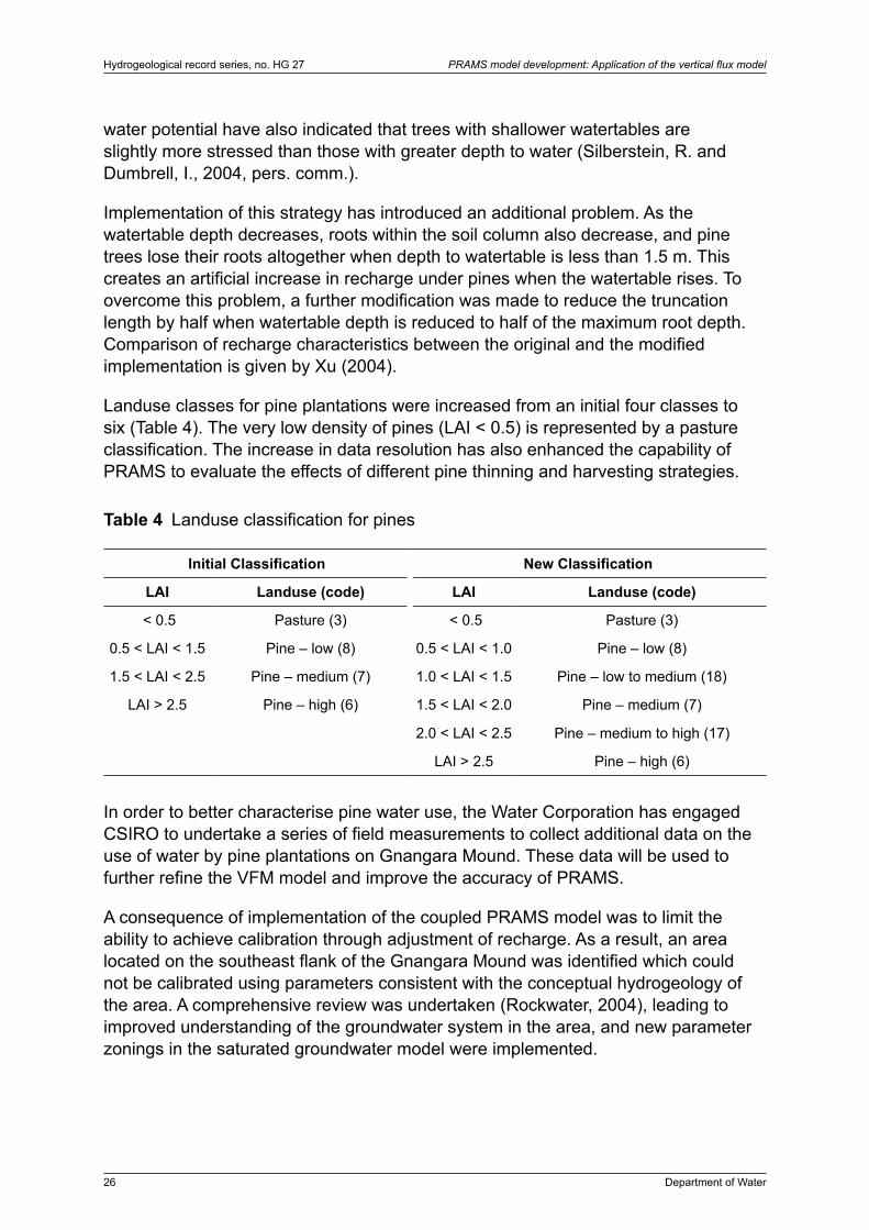
26 Department of Water
Hydrogeological record series, no. HG 27 PRAMS model development: Application of the vertical flux model
water potential have also indicated that trees with shallower watertables are slightly more stressed than those with greater depth to water (Silberstein, R. and Dumbrell, I., 2004, pers. comm.).
Implementation of this strategy has introduced an additional problem. As the watertable depth decreases, roots within the soil column also decrease, and pine trees lose their roots altogether when depth to watertable is less than 1.5 m. This creates an artificial increase in recharge under pines when the watertable rises. To overcome this problem, a further modification was made to reduce the truncation length by half when watertable depth is reduced to half of the maximum root depth. Comparison of recharge characteristics between the original and the modified implementation is given by Xu (2004).
Landuse classes for pine plantations were increased from an initial four classes to six (Table 4). The very low density of pines (LAI < 0.5) is represented by a pasture classification. The increase in data resolution has also enhanced the capability of PRAMS to evaluate the effects of different pine thinning and harvesting strategies.
Table 4 Landuse classification for pines
Initial Classification New Classification
LAI Landuse (code) LAI Landuse (code)
< 0.5 Pasture (3) < 0.5 Pasture (3)
0.5 < LAI < 1.5 Pine – low (8) 0.5 < LAI < 1.0 Pine – low (8)
1.5 < LAI < 2.5 Pine – medium (7) 1.0 < LAI < 1.5 Pine – low to medium (18)
LAI > 2.5 Pine – high (6) 1.5 < LAI < 2.0 Pine – medium (7)
2.0 < LAI < 2.5 Pine – medium to high (17)
LAI > 2.5 Pine – high (6)
In order to better characterise pine water use, the Water Corporation has engaged CSIRO to undertake a series of field measurements to collect additional data on the use of water by pine plantations on Gnangara Mound. These data will be used to further refine the VFM model and improve the accuracy of PRAMS.
A consequence of implementation of the coupled PRAMS model was to limit the ability to achieve calibration through adjustment of recharge. As a result, an area located on the southeast flank of the Gnangara Mound was identified which could not be calibrated using parameters consistent with the conceptual hydrogeology of the area. A comprehensive review was undertaken (Rockwater, 2004), leading to improved understanding of the groundwater system in the area, and new parameter zonings in the saturated groundwater model were implemented.
Department of Water 27
PRAMS model development: Application of the vertical flux model Hydrogeological record series, no. HG 27
2.7.2 Excessive recharge in the Guildford soil under pasture
Using the recommended soil hydraulic properties, WAVES generates water yields of 30–40% of rainfall beneath pasture in the area of Guildford soil. This is a reasonable estimate when compared with modelling results and field data from other catchment water balances in similar areas of Australia (e.g. Zhang et al., 2001). However, the area with the Guildford soil has groundwater close to the surface. As a result, part of the water yield is rejected from the aquifer because it is full (referred to as ‘rejected recharge’ in the literature) and ponds on the surface. This contributes to additional EVT and surface runoff. As both MODFLOW and the VFM do not handle this type of runoff, groundwater levels increase above the ground level when the ‘rejected recharge’ is applied to the model. This generates systematic errors in these areas. Introduction of more detailed drainage features to the model alleviates the problem only to some extent, owing to the low permeability of the underlying (saturated) Guildford clay, and considerable errors occurred in some areas.
To resolve the issue without introducing complex models to handle the groundwater surface water interaction in the VFM, the saturated hydraulic conductivity of Guildford soil was reduced as part of model calibration. The calibrated hydraulic conductivity for the Guildford soil is 0.01 m/d, which is significantly lower than the value of 0.65 m/d derived from AgWA datasets. This adjustment effectively removes the rejected recharge from the model.
2.7.3 Landuse classes for native woodlands and nominal LAI
The native woodlands were originally classified into three types based on LAI derived from Landsat data: very low, low and high density for LAI < 0.5, 0.5 < LAI < 0.8, and LAI > 0.8 respectively (Table 5). The very low-density banksia was grouped with pasture to reduce the number of RRUs required to run WAVES. The nominal LAI used for low- and high-density banksia in the WAVES simulation was 0.7 and 1.0 respectively. This was adequate for the pilot study. However, when applied to the full-scale model, recharge in the area north of Pinjar was high and simulated heads were consistently higher than observed. In addition, simulated hydrographs indicated that the recharge response was too rapid compared with observations, particularly when classification changes occur.
To address this, the landuse for banksia woodlands was reclassified into four classes: very low (LAI < 0.5 modelled as pasture), low (0.5 < LAI < 0.75), medium (0.75 < LAI < 0.85) and high (LAI > 0.85) density (Table 5). However, a reasonable calibration can not be achieved if the nominal LAI used for WAVES simulation is constrained within the revised range, particularly for the medium and high class owing to too much recharge in the area north of Pinjar.
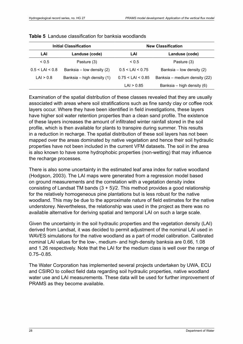
28 Department of Water
Hydrogeological record series, no. HG 27 PRAMS model development: Application of the vertical flux model
Table 5 Landuse classification for banksia woodlands
Initial Classification New Classification
LAI Landuse (code) LAI Landuse (code)
< 0.5 Pasture (3) < 0.5 Pasture (3)
0.5 < LAI < 0.8 Banksia – low density (2) 0.5 < LAI < 0.75 Banksia – low density (2)
LAI > 0.8 Banksia – high density (1) 0.75 < LAI < 0.85 Banksia – medium density (22)
LAI > 0.85 Banksia – high density (6)
Examination of the spatial distribution of these classes revealed that they are usually associated with areas where soil stratifications such as fine sandy clay or coffee rock layers occur. Where they have been identified in field investigations, these layers have higher soil water retention properties than a clean sand profile. The existence of these layers increases the amount of infiltrated winter rainfall stored in the soil profile, which is then available for plants to transpire during summer. This results in a reduction in recharge. The spatial distribution of these soil layers has not been mapped over the areas dominated by native vegetation and hence their soil hydraulic properties have not been included in the current VFM datasets. The soil in the area is also known to have some hydrophobic properties (non-wetting) that may influence the recharge processes.
There is also some uncertainty in the estimated leaf area index for native woodland (Hodgson, 2003). The LAI maps were generated from a regression model based on ground measurements and the correlation with a vegetation density index consisting of Landsat TM bands (3 + 5)/2. This method provides a good relationship for the relatively homogeneous pine plantations but is less robust for the native woodland. This may be due to the approximate nature of field estimates for the native understorey. Nevertheless, the relationship was used in the project as there was no available alternative for deriving spatial and temporal LAI on such a large scale.
Given the uncertainty in the soil hydraulic properties and the vegetation density (LAI) derived from Landsat, it was decided to permit adjustment of the nominal LAI used in WAVES simulations for the native woodland as a part of model calibration. Calibrated nominal LAI values for the low-, medium- and high-density banksia are 0.66, 1.08 and 1.26 respectively. Note that the LAI for the medium class is well over the range of 0.75–0.85.
The Water Corporation has implemented several projects undertaken by UWA, ECU and CSIRO to collect field data regarding soil hydraulic properties, native woodland water use and LAI measurements. These data will be used for further improvement of PRAMS as they become available.

Department of Water 29
PRAMS model development: Application of the vertical flux model Hydrogeological record series, no. HG 27
2.7.4 Enhanced simulated hydrograph
In general, simulated hydrographs at calibration bores follow the correct trends but seasonal variations tend to have a greater amplitude than the observed. To address this, the saturated hydraulic conductivity for the subsoil of Bassendean and Spearwood soils was adjusted as part of model calibration. This resulted in reduction of saturated hydraulic conductivity for Bassendean subsoil from 15 m/d to 10 m/d, and for Spearwood subsoil from 10 m/d to 5 m/d. This is within the range of expected values, particularly in the presence of vertical flow in a profile containing lower conductivity layers.
In summary, key changes made to the VFM data and models during calibration of the pilot and PRAMS 3.0 models are:
• increase the resolution of landuse classes for pine plantation and banksia woodland
• reduce the saturated hydraulic conductivity for the Guildford, Bassendean and Spearwood soils
• allow the nominal LAI used in WAVES simulation for banksia landuse classes to be adjusted as a part of model calibration
• reduce pine water use by truncating the roots at a specified height above the watertable.
With these improvements, the pilot model and full-scale models demonstrate that the VFM and coupled model represents relevant conditions on the Swan Coastal Plain to an acceptable level (CyMod, 2003, 2004).
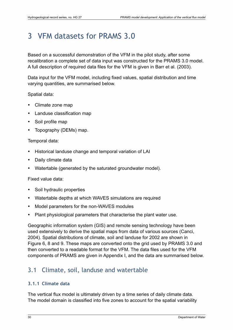
30 Department of Water
Hydrogeological record series, no. HG 27 PRAMS model development: Application of the vertical flux model
3 VFM datasets for PRAMS 3.0
Based on a successful demonstration of the VFM in the pilot study, after some recalibration a complete set of data input was constructed for the PRAMS 3.0 model. A full description of required data files for the VFM is given in Barr et al. (2003).
Data input for the VFM model, including fixed values, spatial distribution and time varying quantities, are summarised below.
Spatial data:
• Climate zone map
• Landuse classification map
• Soil profile map
• Topography (DEMs) map.
Temporal data:
• Historical landuse change and temporal variation of LAI
• Daily climate data
• Watertable (generated by the saturated groundwater model).
Fixed value data:
• Soil hydraulic properties
• Watertable depths at which WAVES simulations are required
• Model parameters for the non-WAVES modules
• Plant physiological parameters that characterise the plant water use.
Geographic information system (GIS) and remote sensing technology have been used extensively to derive the spatial maps from data of various sources (Canci, 2004). Spatial distributions of climate, soil and landuse for 2002 are shown in Figure 6, 8 and 9. These maps are converted onto the grid used by PRAMS 3.0 and then converted to a readable format for the VFM. The data files used for the VFM components of PRAMS are given in Appendix I, and the data are summarised below.
3.1 Climate, soil, landuse and watertable
3.1.1 Climate data
The vertical flux model is ultimately driven by a time series of daily climate data. The model domain is classified into five zones to account for the spatial variability
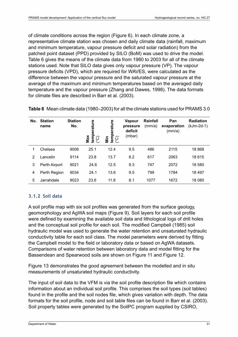
Department of Water 31
PRAMS model development: Application of the vertical flux model Hydrogeological record series, no. HG 27
of climate conditions across the region (Figure 6). In each climate zone, a representative climate station was chosen and daily climate data (rainfall, maximum and minimum temperature, vapour pressure deficit and solar radiation) from the patched point dataset (PPD) provided by SILO (BoM) was used to drive the model. Table 6 gives the means of the climate data from 1980 to 2003 for all of the climate stations used. Note that SILO data gives only vapour pressure (VP). The vapour pressure deficits (VPD), which are required for WAVES, were calculated as the difference between the vapour pressure and the saturated vapour pressure at the average of the maximum and minimum temperatures based on the averaged daily temperature and the vapour pressure (Zhang and Dawes, 1998). The data formats for climate files are described in Barr et al. (2003).
Table 6 Mean climate data (1980–2003) for all the climate stations used for PRAMS 3.0
No. Station name
Station No.
Max
te
mpe
ratu
re
(°C
)
Min
te
mpe
ratu
re
(°C
)Vapour
pressure deficit (mbar)
Rainfall (mm/a)
Pan evaporation
(mm/a)
Radiation (kJm-2d-1)
1 Chelsea 9006 25.1 12.4 9.5 486 2115 18 868
2 Lancelin 9114 23.8 13.7 8.2 617 2063 18 615
3 Perth Airport 9021 24.6 12.5 9.3 747 2072 18 580
4 Perth Region 9034 24.1 13.6 9.5 799 1784 18 497
5 Jarrahdale 9023 23.6 11.8 8.1 1077 1672 18 080
3.1.2 Soil data
A soil profile map with six soil profiles was generated from the surface geology, geomorphology and AgWA soil maps (Figure 9). Soil layers for each soil profile were defined by examining the available soil data and lithological logs of drill holes and the conceptual soil profile for each soil. The modified Campbell (1985) soil hydraulic model was used to generate the water retention and unsaturated hydraulic conductivity table for each soil class. The model parameters were derived by fitting the Campbell model to the field or laboratory data or based on AgWA datasets. Comparisons of water retention between laboratory data and model fitting for the Bassendean and Spearwood soils are shown on Figure 11 and Figure 12.
Figure 13 demonstrates the good agreement between the modelled and in situ measurements of unsaturated hydraulic conductivity.
The input of soil data to the VFM is via the soil profile description file which contains information about an individual soil profile. This comprises the soil types (soil tables) found in the profile and the soil nodes file, which gives variation with depth. The data formats for the soil profile, node and soil table files can be found in Barr et al. (2003). Soil property tables were generated by the SoilPC program supplied by CSIRO,
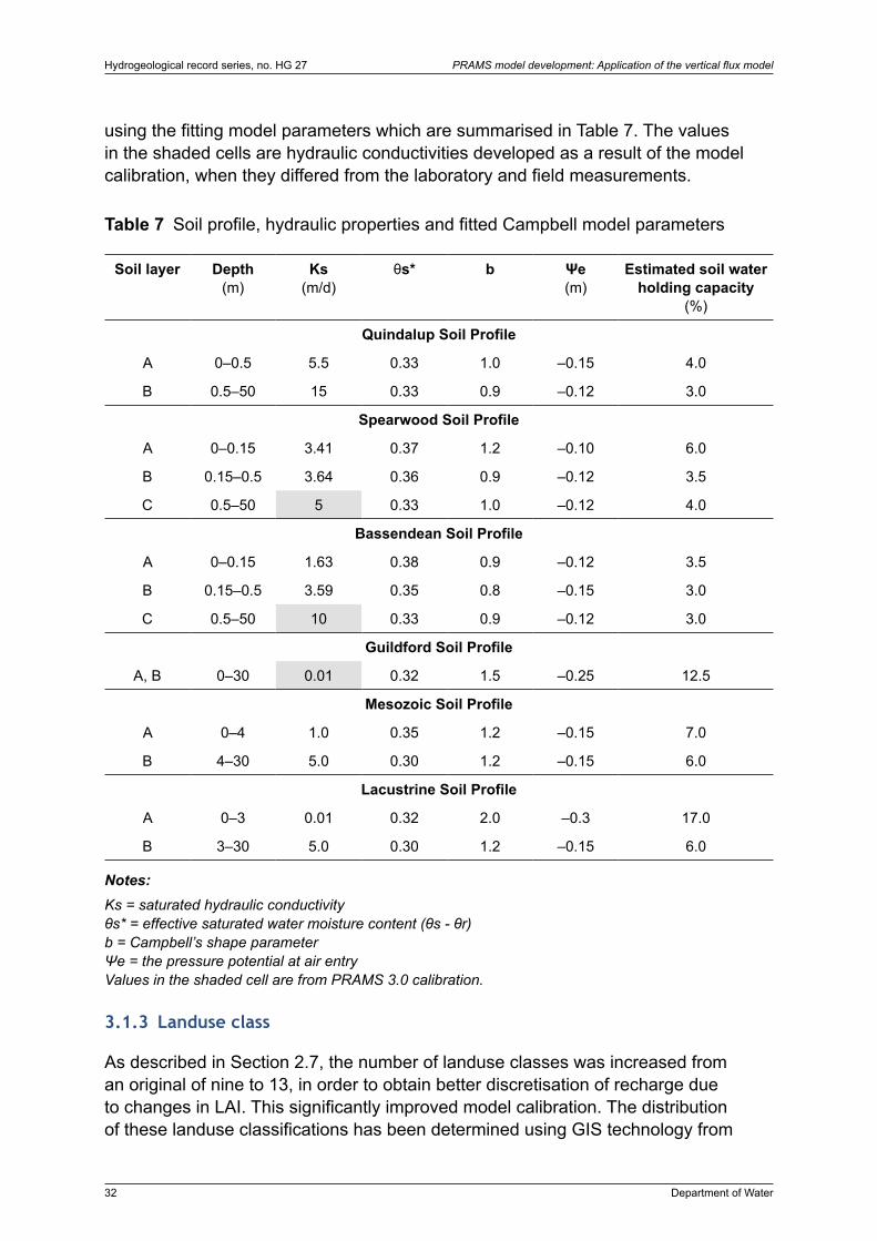
32 Department of Water
Hydrogeological record series, no. HG 27 PRAMS model development: Application of the vertical flux model
using the fitting model parameters which are summarised in Table 7. The values in the shaded cells are hydraulic conductivities developed as a result of the model calibration, when they differed from the laboratory and field measurements.
Table 7 Soil profile, hydraulic properties and fitted Campbell model parameters
Soil layer Depth (m)
Ks (m/d)
θs* b Ψe (m)
Estimated soil water holding capacity
(%)
Quindalup Soil Profile
A 0–0.5 5.5 0.33 1.0 –0.15 4.0
B 0.5–50 15 0.33 0.9 –0.12 3.0
Spearwood Soil Profile
A 0–0.15 3.41 0.37 1.2 –0.10 6.0
B 0.15–0.5 3.64 0.36 0.9 –0.12 3.5
C 0.5–50 5 0.33 1.0 –0.12 4.0
Bassendean Soil Profile
A 0–0.15 1.63 0.38 0.9 –0.12 3.5
B 0.15–0.5 3.59 0.35 0.8 –0.15 3.0
C 0.5–50 10 0.33 0.9 –0.12 3.0
Guildford Soil Profile
A, B 0–30 0.01 0.32 1.5 –0.25 12.5
Mesozoic Soil Profile
A 0–4 1.0 0.35 1.2 –0.15 7.0
B 4–30 5.0 0.30 1.2 –0.15 6.0
Lacustrine Soil Profile
A 0–3 0.01 0.32 2.0 –0.3 17.0
B 3–30 5.0 0.30 1.2 –0.15 6.0
Notes:Ks = saturated hydraulic conductivity θs* = effective saturated water moisture content (θs - θr) b = Campbell’s shape parameter Ψe = the pressure potential at air entry Values in the shaded cell are from PRAMS 3.0 calibration.
3.1.3 Landuse class
As described in Section 2.7, the number of landuse classes was increased from an original of nine to 13, in order to obtain better discretisation of recharge due to changes in LAI. This significantly improved model calibration. The distribution of these landuse classifications has been determined using GIS technology from

Department of Water 33
PRAMS model development: Application of the vertical flux model Hydrogeological record series, no. HG 27
satellite imagery, air photographs, cadastral and other mapping information. Historical landuse maps were generated for 1985 and 1988–2002 in two–year intervals using Landsat data (Appendix II). Table 8 lists the landuse classes together with the VFM modules used for recharge estimates.
Table 8 Landuse classification and recharge module used
Landuse code
Description VFM module
1 Banksia – high density WAVES
22 Banksia – medium density WAVES
2 Banksia – low density WAVES
3 Pasture WAVES
5 Market garden /parkland LINEAR
6 Pine – high density WAVES
17 Pine – medium to high density WAVES
7 Pine – medium density WAVES
18 Pine – low to medium density WAVES
8 Pine – low density WAVES
9 Urban residential LINEAR
10 Lakes/wetlands PIECEWISE LINEAR
11 Urban commercial/industrial LINEAR
3.1.4 Watertable depths
Watertable depth at a particular site is determined by the surface elevation and the level of the watertable, which is provided by the saturated groundwater model through the dynamic link between the MODFLOW and VFM. However, because the efficiencies gained in selecting the RRU would otherwise be lost, the WAVES simulations are run for a subset of watertable depths. Recharge at a site whose watertable depth falls between any two of these designated depths is estimated by interpolation from the simulation results at those depths.
Sensitivity analysis indicates that recharge is more sensitive to water level change when the watertable is close to the surface. Small intervals were used to capture the dynamic response of recharge and watertable change in the shallow depth to watertable ranges. In PRAMS 3.0, WAVES is simulated at eight watertable depths: 0.1, 1.0, 2.0, 4.0, 6.0, 10.0, 15.0 and 50.0 m.
34 Department of Water
Hydrogeological record series, no. HG 27 PRAMS model development: Application of the vertical flux model
3.2 Models and parameters for VFM recharge modules
As discussed earlier, the VFM package has two types of recharge models to calculate net recharge due to precipitation: WAVES, and simple algebraic models based on rainfall and pan evaporation only. The latter can have either a simple LINEAR model or a more complex PIECEWISE_LINEAR model. The LINEAR model uses constant coefficients for the rainfall and evaporation, whereas the PIECEWISE_LINEAR model allows the coefficients to be piecewise linear functions of watertable depth.
3.2.1 WAVES
For the landuse classifications of banksia woodland, pine plantation and pasture, VFM uses WAVES to calculate the net rainfall recharge (Table 8). These classifications represent about 90% of the onshore model domain. WAVES landuse files contain all information required for WAVES simulation including the LAI, litter, root carbon distribution and the vegetation parameter file that characterises the plant water use features of particular species. The data format for these files can be found in Barr et al. (2003).
WAVES is a process-based model requiring 26 vegetation parameters to fully describe canopy energy and carbon balance, canopy and root growth, and interactions between soil and vegetation. The vegetation growth capability of WAVES is not implemented in the VFM and only 16 parameters are required to represent the key processes in the Perth region. Most of these parameters can be measured directly or taken from plant physiological literature, with only a few requiring fitting or adapting to local conditions. Vegetation parameters used in the VFM for pines, native banksia woodlands and pasture are listed in Appendix III. Details on how they have been derived are described by Silberstein et al. (2004). Other important parameters including root depth and distribution, LAI and litter load are described below.
3.2.1.1 Root depth and distribution
Previous studies on the Gnangara Mound (Dodd and Bell, 1993a,b; Farrington and Bartle, 1991; Sharma et al., 1991a) showed that roots of banksia woodlands penetrate to depths of 8–10 m below ground level. Recent field data from the McLarty Plantation (Bekele and Silberstein, 2003) indicate that the roots of Pinus pinaster can exceed 12 m depth. As a result, in PRAMS 3.0, maximum root depths for pines and native woodlands are set to 12 m and 10 m respectively. For annual pasture, the maximum root depth is set to 1.0 m.
Root distribution in the soil profile for each vegetation species is specified in the root input file. For banksia woodlands, the rooting density uses a logarithmic decay to a maximum rooting depth. Traditionally models of root density have often used an exponential decay function with depth (e.g. Gardner, 1991). However, it was found that this limits the native banksia’s access to deeper groundwater, particularly in times of drought. The logarithmic function instead attempts to mimic the architecture
Department of Water 35
PRAMS model development: Application of the vertical flux model Hydrogeological record series, no. HG 27
of root structure in native vegetation. This is considered to provide the ability to extract water more evenly from the soil profile and increase drought tolerance. For pines, an exponential decay function is used, reflecting the fact that we believe they are less tolerant of drought conditions.
Figure 14 shows the root density distribution for banksia woodland and pines. For annual pasture, roots are grown to the maximum root depth with an exponential decaying function.
The VFM also introduces a new parameter to truncate the roots above the watertable to simulate the effects of a moving watertable. This only applies to pine, since there is evidence to indicate that native banksia woodlands are capable of extracting groundwater when their roots intercept groundwater (Froend et al., 1999).
3.2.1.2 LAI
With the exception of annual pasture, all landuse classes employing WAVES use a constant leaf area index (LAI) throughout the simulation. For pine plantation, the nominal LAI used in WAVES simulations is the median of the range used to define the class from Landsat data. For example, the range of pine LAI for medium density is 1.5–2.0 and a nominal LAI of 1.75 is used in the simulation for this landuse class. For banksia woodland, the nominal LAIs were determined by model calibration as discussed in Section 2.7. LAIs used for WAVES simulation for landuse classes of pines and banksia woodlands are given in Table 9.
In the landuse file, the leaf carbon value is required instead of LAI. Conversion of LAI into leaf carbon is achieved by dividing the LAI by specific leaf area. The specific leaf areas used in the current implementation are 6 LAI/kg C for banksia woodlands, 10 LAI/kg C for pines and 24 LAI/kg C for annual pasture. These values apply for LAI conversion and have no material effect on the water balance as they are essentially rescaling leaf coverage in the VFM.
For annual pasture, an annual trend of LAI is assigned that follows normal pasture growth and senescence in monthly increments. The maximum LAI has been adjusted during PRAMS 3.0 calibration. The calibrated maximum LAI for pasture is 3.0 and the annual profile is shown in Figure 15.
3.2.1.3 Litter
WAVES can simulate litter interception, a process where rainfall is retained in litter and evaporated without adding water to the underlying soil. The amount of litter measured in kilograms of carbon per square metre can be specified in the landuse file.
Litter accumulation at a particular site depends on the vegetation density, fire history and other human intervention such as pine thinning. In the areas with pine plantations and native woodland, the responsibility of land management is with the

36 Department of Water
Hydrogeological record series, no. HG 27 PRAMS model development: Application of the vertical flux model
Department of Environment and Conversation (DEC). Prescribed burnings, which are carried out during spring and autumn, are normally used to reduce the build-up of leaves and twigs on the land surface. A recent study revealed that the frequency of burning has reduced significantly from two- to four-year intervals before about 1880 to more than 10-year intervals over the last two decades, with some locations being unburnt for over thirty years (Ward et al., 2004).
There are insufficient data to generate the spatial and temporal distributions of litter accumulation for the study area. Early work by Farrington and Bartle (1991) indicated that at their pine investigation site, litter accumulation was up to 2.5 cm deep and amounted to 20 tonnes of dry matter per hectare. This may be an extreme case occurring in high density of pines that had not been burnt for some time. For PRAMS modelling, the litter load for the medium- to high-density pines is assumed to be 10 t/ha, whereas for low- to medium- and low-density classes a value of 5 t/ha is used. It should be noted that for the landuse classes with high LAIs, the prescribed litter load has very little impact on the recharge, since water that is not intercepted by the litter and infiltrates into the soil would otherwise be used by the plant via transpiration.
Farrington and Bartle (1991) work also found that the litter accumulation in the native banksia woodlands is much less than in dense pine plantation. A study by DEC (Figure 16 ) shows that ground litter in the banksia woodlands near Perth accumulates at a rate of half a ton per hectare per year for the first five years after a fire event and then stabilises at around 2.5 t/ha. For PRAMS modelling, the ground litter load for medium-and high- density banksia is assumed to be 2.5 t/ha and 1.0 t/ha for the low- density class.
For annual pasture, litter accumulation is assumed to be small and is set at zero. This should have no significant effect on the water balance as LAIs for the annual pasture are determined during model calibration and will implicitly account for litter.
Table 9 Nominal LAI and litter load for vegetation landuse classes
Landuse code
Description Nominal LAI Litter (t/ha)
1 Banksia – high density 1.26* 2.5
22 Banksia – medium density 1.08 2.5
2 Banksia – low density 0.66 1.0
3 Pasture 0–3 (LAI file) 0
6 Pine – high density 2.75 10
17 Pine – medium to high density 2.25 10
7 Pine – medium density 1.75 10
18 Pine – low to medium density 1.25 5
8 Pine – low density 0.75 5
*Values in the shaded cell are results of PRAMS 3.0 calibration
Department of Water 37
PRAMS model development: Application of the vertical flux model Hydrogeological record series, no. HG 27
3.2.2 Algebraic models
For the urban, market garden/parkland and lakes/wetland, the VFM uses the simple algebraic models to calculate the net rainfall recharge for PRAMS 3.0. Starting from the initial values given in Table 3, parameters were refined as part of PRAMS 3.0 calibrations to minimise the difference between the observed and simulated hydrograph. Table 10 gives the calibrated parameters for each landuse classification.
Table 10 Calibrated model parameters for algebraic models
Landuse code
Description VFM module Rainfall Coef.
α
EVT Coef.
β
EVT extinction depth
(m)
5 Market garden/parkland
LINEAR 0.4 0 n/a
9 Urban residential LINEAR 0.62 0.05 n/a
10 Lakes/wetlands PIECEWISE LINEAR 1.1 0.75 3.0
11 Urban commercial and industrial
LINEAR 0.75 0.05 n/a
For the urban residential areas, model calibration gives a recharge rate of about 50% rainfall. The corresponding values for the parameters α and β are 0.62 and 0.05 respectively. In the commercial and industrial areas, the calibration gives a recharge rate of about 63%. The corresponding values for the parameters α and β are 0.75 and 0.05 respectively. The resulting recharge rates using these calibrated values are consistent with the empirical estimates given in Table 3.
For parkland/market garden, the VFM uses the recommended coefficient 0.4 for α, which means net rainfall recharge is 40% of rainfall.
For lakes and wetland, PRAMS 3.0 calibration uses a coefficient of 1.1 for rainfall to account for additional inflows from the surrounding area. Evaporation from the water surface is assumed to be 0.75 of pan evaporation and reduced linearly to zero when the groundwater level falls 3 m below the ground surface. The evaporation coefficient used is slightly lower than the value of 0.80 to 0.85 recommended by AgWA for the Perth region (Luke et al., 1987) but this low value is used in the model calibration to reduce the seasonal variations in the simulated hydrograph to match the actual observations. With these model parameters, the area inundated permanently will be a groundwater evaporation basin with net discharge of about 0.5 m per year.
38 Department of Water
Hydrogeological record series, no. HG 27 PRAMS model development: Application of the vertical flux model
4 Model applications
The new VFM has been integrated with the MODFLOW-based saturated groundwater model. The coupled calibrated model is designated as PRAMS 3.0. The hydrogeology and conceptual model for the saturated model are described in detail by Davidson and Yu (2004). Full model implementation and calibration are described by CyMod (2004).
PRAMS 3.0 covers an area of 11 000 km2 of the Perth region between Mandurah in the south and Wedge Island in the north (Figure 1). About 9000 km2 of this area is onshore and the remainder is offshore. The model represents the entire major aquifer and aquitard systems to a depth of more than 2000 m. Horizontally, the model uses a uniform grid of 500 by 500 m over the entire model domain. Vertically, the model has 12 layers with each layer representing an aquifer (or part thereof) or aquitard (Yu et al., 2002). Figure 17 shows the structure of PRAMS 3.0, illustrating the water balance components being incorporated in the model.
Only the onshore part of the model domain requires recharge calculation. To facilitate passing of fluxes between the saturated groundwater model and VFM, and to ensure that the water balance is maintained, the VFM uses the same uniform grid as the saturated model. Gridded maps for climate, landuse and soil profiles together with a set of watertable depths were prepared and used for the RRU classifications. Theoretically, there are 3120 RRUs (5 climates × 13 landuse (but only 9 classes use WAVES) × 6 soil profiles × 8 watertable depths) for the whole model domain. Of these, 2160 RRUs may be used by WAVES; the remainder apply simpler linear models. However, not all combinations occur within the model domain and the VFM automatically determines and discards RRUs that are not used. In this application, only about 750 RRUs were simulated by WAVES. For the non-WAVES RRUs, the VFM calculates the recharge on a cell by cell basis.
Results from application of the VFM to the Perth region using the data as described previously are presented at two levels. The first level reports the results from (typical) individual RRUs (plot scale) with details on the components of the water balance. Results are also compared with published data where possible. Note that although there have been many studies on recharge in the Perth region, it is difficult to compare these studies with the current modelling results, since most of the datasets lack sufficient detail on the site conditions, particularly soil and vegetation data, to allow a valid comparison. The second level reports recharge estimates on a regional scale, giving an overall picture of the spatial and temporal variation of groundwater recharge for different areas of interest. This was done by undertaking detailed water balance analysis using data generated by PRAMS 3.0, over the simulation period to account for landuse changes and interaction between recharge and groundwater level.

Department of Water 39
PRAMS model development: Application of the vertical flux model Hydrogeological record series, no. HG 27
4.1 Results from RRU: plot scale simulation
A detailed water balance for each WAVES RRU was obtained by running PRAMS over the period 1980 – 2003 with the WAVES log file output option. These log files give a summary of the critical components of the water balance such as rainfall, storage change, canopy and litter interception loss, soil evaporation, transpiration and deep drainage (recharge) over the simulation period. As discussed previously, recharge is dependent on landuse, climate, soil and watertable depth, and running of the model generates over 750 data files, one for each WAVES RRU. It is impractical to report results of all RRUs, and only some important ones are presented here.
Figure 18 shows the simulation results for pasture, banksia woodland and pine plantations for climate zone 4 (Perth regional office) and Bassendean soil under a range of watertable depths. Recharge is expressed as a percentage of rainfall over the simulation period (average 800 mm per annum). Negative recharge means the evapotranspiration is greater than rainfall and that groundwater discharge instead of net recharge occurs for the RRU.
Under pasture, the recharge rate is estimated to be about 45% of rainfall. Sharma et al. (1991a) investigated recharge under pasture at two sites north of Perth using hydrograph analysis and a chloride balance method and found that the recharge rate was in the range 50–60% of rainfall. The recharge estimated by WAVES is slightly lower but reasonably close to their results. The averaged recharge rate for pasture is almost constant when watertable depth is greater than 2 m. This is because pasture has a shallow root system (maximum root depth set to 1.0 m) and any infiltrated rainfall passing through the root zone will recharge groundwater.
For the banksia woodlands, WAVES estimates that recharge rates for low, medium and high density are about 38%, 18% and 10% respectively in the area with deep watertable. For medium- and high-density classes, recharge rates are reduced slightly as the depth to watertable decreases. Previous field studies to estimate recharge under banksia woodlands using different methods gave a wide range of results extending from 15 to 43% (Thorpe, 1985; Sharma et al., 1991a). A direct comparison between WAVES estimates and these results is difficult since little information on the site conditions, particularly vegetation density, was collected or reported at these sites. Nevertheless, WAVES produces similar estimates of recharge consistent with findings of these earlier studies.
For pine plantations, simulation results indicate that recharge occurs only under low- and low- to medium- density classes with recharge rates of about 28% and 8% respectively. For medium- to high-density pines, there is no recharge in the case of deep watertable and pines may become net users of groundwater, possibly up to 40% of rainfall in the case of shallow depth to watertable. Previous studies using environmental tracers such as chloride and bromide and water balance analysis (Sharma et al.,1991a; Farrington and Bartle, 1991; and Butcher, 1979) indicated that recharge under young pines could be as high as 30% of rainfall, but may be zero
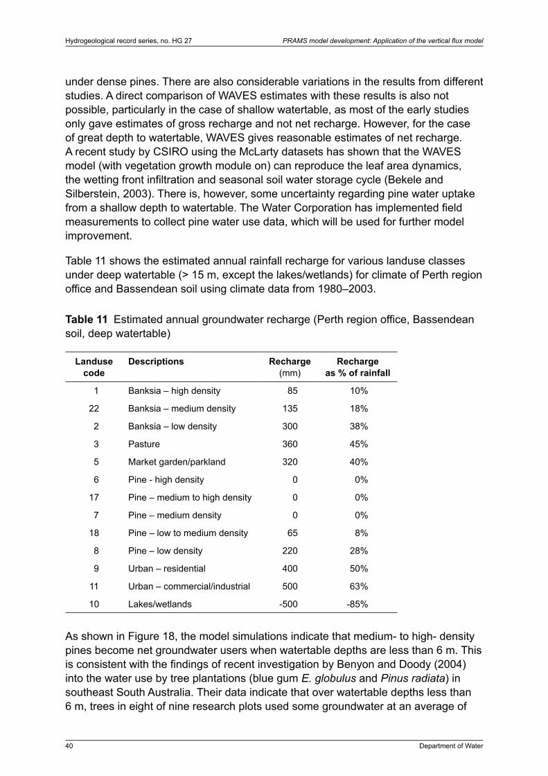
40 Department of Water
Hydrogeological record series, no. HG 27 PRAMS model development: Application of the vertical flux model
under dense pines. There are also considerable variations in the results from different studies. A direct comparison of WAVES estimates with these results is also not possible, particularly in the case of shallow watertable, as most of the early studies only gave estimates of gross recharge and not net recharge. However, for the case of great depth to watertable, WAVES gives reasonable estimates of net recharge. A recent study by CSIRO using the McLarty datasets has shown that the WAVES model (with vegetation growth module on) can reproduce the leaf area dynamics, the wetting front infiltration and seasonal soil water storage cycle (Bekele and Silberstein, 2003). There is, however, some uncertainty regarding pine water uptake from a shallow depth to watertable. The Water Corporation has implemented field measurements to collect pine water use data, which will be used for further model improvement.
Table 11 shows the estimated annual rainfall recharge for various landuse classes under deep watertable (> 15 m, except the lakes/wetlands) for climate of Perth region office and Bassendean soil using climate data from 1980–2003.
Table 11 Estimated annual groundwater recharge (Perth region office, Bassendean soil, deep watertable)
Landuse code
Descriptions Recharge (mm)
Recharge as % of rainfall
1 Banksia – high density 85 10%
22 Banksia – medium density 135 18%
2 Banksia – low density 300 38%
3 Pasture 360 45%
5 Market garden/parkland 320 40%
6 Pine - high density 0 0%
17 Pine – medium to high density 0 0%
7 Pine – medium density 0 0%
18 Pine – low to medium density 65 8%
8 Pine – low density 220 28%
9 Urban – residential 400 50%
11 Urban – commercial/industrial 500 63%
10 Lakes/wetlands -500 -85%
As shown in Figure 18, the model simulations indicate that medium- to high- density pines become net groundwater users when watertable depths are less than 6 m. This is consistent with the findings of recent investigation by Benyon and Doody (2004) into the water use by tree plantations (blue gum E. globulus and Pinus radiata) in southeast South Australia. Their data indicate that over watertable depths less than 6 m, trees in eight of nine research plots used some groundwater at an average of

Department of Water 41
PRAMS model development: Application of the vertical flux model Hydrogeological record series, no. HG 27
435 mm/year. They also found that maximum depth to watertable for groundwater uptake is approximately 6 m. However, their results may have limited application to the Swan Coastal Plain owing to different tree species (Pinus radiata vs Pinus pinaster) and site conditions. There are only small areas near Lexia where the current watertable depth under pine plantations is less than 6 m. Therefore, the uncertainty in pine water use under shallow watertable should not have a significant effect on the simulation of regional groundwater fluxes.
Individual components of the water balance were also examined. Figure 19 illustrates how the four key components of the water balance, namely, canopy interception loss, litter interception and soil evaporation, plant transpiration and deep drainage (recharge) vary for different classes of landuse. In the cases shown, depth to watertable is greater than 15 m. As expected, the canopy interception loss increases with increasing vegetation density (LAI). Interception loss for banksia woodland ranges from 7% of rainfall for low density to 12% for high density.
For the pine plantation, canopy interception loss is higher and up to 21% of rainfall is lost for the high density class. These values are consistent with those previously reported on the Swan Coastal Plain (SCP) or in literature (Hatton et al., 2001). Similarly, simulated litter interception and soil evaporation (mainly the litter interception) is also much higher under pine plantations, particularly for the medium to high density classes, with up to 28% of rainfall compared with about 12% for banksia woodland. Modelling results also indicate that for the area with deep watertable, medium and high density native bush transpires more water than the medium to high density pines. This is because in areas with deep watertable the transpiration is limited by soil water availability. Under the dense pines, the canopy and litter interception are much higher so less rainfall is available to infiltrate into the soil.
Simulation results indicate that recharge gradually reduces to zero when plant LAI reaches about 1.5–2.0 depending on litter loads. This is consistent with recent work by Ellis et al. (1999) who examined vegetation and climate data from a number of published studies around southern Australia. They developed a relationship between the long-term ‘equilibrium’ LAI and a climate ‘wetness index (P/Ep)’, namely:
LAI = 2.9 × P/Ep (4)
where
P = annual total precipitation, and
Ep = annual total potential evaporation.
The term ‘equilibrium’ means that the LAI developed is in dynamic equilibrium with the long-term climate. This assumes that the vegetation has evolved to a condition in which it optimises its water use for long-term survival in conditions of highly seasonal rainfall and episodic drought. Using the average rainfall of 800 mm/a and potential

42 Department of Water
Hydrogeological record series, no. HG 27 PRAMS model development: Application of the vertical flux model
evaporation of 0.8 times the pan evaporation of 1780 mm/a (Perth region office) gives an ‘optimal’ LAI value of about 1.65 .
Recharge is also affected by the soil characteristics. Figure 20 shows recharge for different landuse classes under the same climate regimes (Perth region office) but in an area with Spearwood soil. The figure shows a similar pattern to that in Figure 18 but the recharge rate is 3–5% lower than the case with Bassendean soil. This is because Spearwood soil has better soil water holding capacity and is capable of storing more winter rainfall for plant use late in summer when evaporative demand is high. Simulation results indicate that recharge in the areas of Quindalup soil is similar to that of Bassendean soil. For the Guildford soil, the major landuse is pasture and recharge is about 10% with deep watertable; and it becomes net discharge in areas with shallow watertable.
Recharge under different climate regimes was also examined. Figure 21 shows the simulation results for pasture and banksia in the area of Bassendean soil for climate zones 2–5 (no Bassendean soil in climate zone 1). The average annual rainfall ranges from 617 mm (climate zone 2) to 1078 mm (climate zone 5) for the simulation period. As expected, recharge increases with increasing rainfall but the slope of increase is steeper in the high rainfall regime. For medium and high density banksia woodlands, there would be almost no recharge when rainfall falls below 600 mm/a. However, should there be a systematic decline in rainfall, a significant shift toward more xeric vegetation communities would also be expected, which use less water thereby allowing slightly more recharge.
In the Gingin area, simulated recharge is about 180 mm/a for annual pasture, 150 mm/a for low-banksia woodlands and almost no recharge for the medium and high density banksia woodlands. On the Dandaragan Plateau, the recharge rate for annual pasture is about 100 mm/a with almost no recharge under banksia woodland.
4.2 Simulation results on a regional scale
VFM simulation results can be upscaled into different regions of interests. To account for the dynamic nature of landuse and interaction between depth to watertable and groundwater recharge, detailed water balance analysis using cell by cell budget files from the coupled model (PRAMS 3.0) was carried out. The model was set up to start from January 1980 and finish in December 2003 with the first five years run to establish initial conditions. Data from 1985 to 2003 were used for this analysis. To alleviate the effects of delay in recharge in the analysis, a fiscal year was used instead of a calendar year.
The PRAMS study area was divided into different zones for analyses, which provides recharge information at different scales under different regimes (climate, soil and landuse etc.). Groundwater recharge is averaged over the area of interest (expressed in mm/a) and given as total recharge in the area (GL per annum).

Department of Water 43
PRAMS model development: Application of the vertical flux model Hydrogeological record series, no. HG 27
4.2.1 Recharge for four regions
The modelling domain is delineated into four regions as shown in Figure 22
• North SCP: North of the Gingin Brook,
• Centre SCP: North of Swan River and South of Gingin Brook,
• South SCP: South of Swan River to Mandurah, and
• Gingin to Dandaragan: between the Gingin and Darling Scarps.
The annual recharge for the four zones over the period from1985 to 2003 is shown in Figure 23 (mm) and Figure 24 (GL). Unless stated otherwise, an average rainfall of 800 mm/a over the period is used as the reference rainfall. Table 12 gives statistics of recharge for each zone. Annual recharge varies significantly from year to year in response to climate and landuse change and average annual recharge for these four areas is 333, 356, 278 and 361 GL respectively. Average annual recharge for the whole study area is about 18% of rainfall. For the south and central area of the SCP, the average annual recharge is about 634 GL or 20% of rainfall.
The current PRAMS calibration focuses on the area between Gingin in the north and Mandurah in the south (Centre and South SCP) and simulation results outside of these areas should be treated with caution due to lack of monitoring data for model calibration and verification.
Table 12 Averaged annual recharge and variation for period 1985–2003
Zone Area (km2 )
Averaged recharge
(GL)
Averaged recharge
(mm)
Coefficient of variation
North SCP 2778 333 120 0.36
Centre SCP 2226 356 160 0.22
South SCP 1705 278 163 0.28
Gingin and Dandaragan 2584 361 140 0.21
ALL domain 9295 1327 143 0.19
4.2.2 Recharge for central area of SCP
More detailed analysis was carried out for the Centre SCP (Figure 22) for different soil types and landuse. Table 13 gives the average annual recharge for different soil types. Recharge rates for the sandy soils (Quindalup, Spearwood and Bassendean) are 259, 220, 192 mm/a respectively. The difference in recharge for these sandy soils is dominated primarily by landuse and watertable depth. Quindalup and Spearwood soils are associated with sand dunes along the coast where the major landuse is urban, and hence these areas have higher recharge. In areas with Bassendean soil, the major landuse is native bush and pine plantations, and the average recharge rate

44 Department of Water
Hydrogeological record series, no. HG 27 PRAMS model development: Application of the vertical flux model
is lower. Guildford and lacustrine soils are commonly present in the lowland areas of the landscape, where the watertable is shallow. Simulation results indicate that these areas become groundwater discharge zones. These results are consistent with the conceptual hydrogeology on the SCP.
Table 13 Annual recharge under different soil type in the centre of SCP
Soil type Area (km2 )
Average recharge (GL)
Average recharge (mm)
Quindalup 145 38 259
Spearwood 722 159 220
Bassendean 915 176 192
Guildford 263 -8 -30
Lacustrine 173 -7 -40
Table 14 gives the results for different landuses based on the landuse map of 2002 for the sandy part (Quindalup, Spearwood and Bassendean soils) of the central area on the SCP. Landuse in the region has varied through the period of simulation (urbanisation, fire, pine thinning and pine growth etc.) and the landuse classes were aggregated to the primary landuse type (see Table 14) as the zoning for water balance analysis to reduce the effects of landuse change. Table 14 shows that recharge is highest in the urban area (400 mm/a or about 50% of rainfall) and becomes negative (discharge) in the lakes and wetlands. Recharge under pasture (245 mm/a or about 30% rainfall) is higher than under banksia woodland (170 mm/a or about 20% of rainfall). Average recharge under pine plantations is significantly lower (67 mm/a or about 8% of rainfall). This value includes the effects of clearing in the late 1980s and does not represent the current recharge condition, which is estimated to be around 5%. It should also be noted that these recharge values are the result of an averaging process over three climate zones and four soil types, and, as such, are not directly comparable with the results presented in the plot scale simulations.
4.2.3 Recharge for central area of Gnangara Mound
Further analysis was carried out for the central Gnangara Mound (Figure 25), an area of 1250 km2 where the underlying groundwater resource is most critical to the security of public water supply, horticultural use and groundwater dependent ecosystems (GDEs). A recent study by DoE using observed data from monitoring bores indicated that groundwater levels in the area have been declining over the last two decades. The rate of decline has increased over the last seven years to a rate equivalent to a storage depletion of 50 GL per annum. The cause for the decline is believed to be the combined effects of reducing rainfall, lack of thinning pines that prevent effective recharge and an increase in public and private abstraction. Changed fire regime is believed to be another contributor, but over a longer time frame.

Department of Water 45
PRAMS model development: Application of the vertical flux model Hydrogeological record series, no. HG 27
Table 14 Annual recharge under different landuse type in the sandy soil in the centre of SCP
Landuse type Area (km2 )
Averaged recharge (GL)
Averaged recharge (mm)
Pasture 294 72 245
Banksia woodland 940 160 170
Pine plantation 220 14 67
Urban 312 125 400
Parkland/market garden 11 3 250
Lakes/wetlands 5 -1 -190
Annual groundwater recharge for the period of 1985–2003 is shown in Figure 26 together with annual rainfall. This figure shows that there is a good correlation between recharge and rainfall. The average annual recharge for the area is about 190 GL per annum. However, annual recharge prior to 1997 was much higher than during the last few years. The average annual recharge for the period 1985–1997 is about 206 GL compared with an average annual recharge of 155 GL for the period of 1997 to 2003, a reduction of about 50 GL, or 25%, accounting for almost all of the storage depletion observed. This analysis indicates that the major cause for water level declines over recent years is the reduction in the rainfall recharge.
Figure 27 shows the annual recharge under pines and other landuses (mainly banksia woodlands). The difference in the recharge rate under these can be used to estimate the effects of pine plantations on the mound. In late 1980 and early 1990, recharge under pines was reasonably high at around 100 mm/a. This was largely due to the effects of land clearing prior to pine planting in the Yanchep area. Recharge under pines over the last few years has been reduced to about 45 mm/a partly due to a lack of thinning and partly due to reduction in rainfall. In the northern area (north of Lake Pinjar), the recharge rate over the last decade is in the range 2–3% of rainfall, whereas recharge to the south (Gnangara and Lexia areas) is about 10% of rainfall. The difference in recharge is mainly due to the density of pines in these two areas with the southern area having a high proportion of low-density pines.
Figure 28 shows the relationship between recharge and rainfall using rainfall data from the BoM Perth region office. As expected, recharge increases with increasing rainfall, but the relationship appears non-linear and is proportionally greater for higher rainfall. The graph does not include low rainfall data, and therefore the relationship between low rainfall recharge is not represented. For groundwater recharge to commence a rainfall threshold would need to be exceeded. Using the same dataset, the cumulative probability distribution of recharge on the mound can be evaluated (Figure 29). This relation may be useful for assessing the available resource using a risk-based management framework.

46 Department of Water
Hydrogeological record series, no. HG 27 PRAMS model development: Application of the vertical flux model
4.2.4 Recharge for groundwater subareas
For local groundwater management, interest may be in the recharge for a designated groundwater area. The simulation results for the period of 1985–2003 can be upscaled to a groundwater subarea. Figure 30 shows the simulated recharge map based on the groundwater subareas defined by DoE with a further subdivision in the Pinjar subarea to increase the resolution.
Average annual recharge ranges from 170 to 400 mm with the highest recharge in the urban areas and the lowest in areas with lakes and wetlands. In general, recharge is higher in areas with deep watertable compared to areas with shallow watertable.
Recharge along the foothills is low compared with other areas. This is because the foothills are commonly associated with the Guildford Clay, which has low permeability and hence less capacity to carry flow, resulting in shallow watertable and high rejected recharge.
Recharge in the Whitfords area is about 330 mm/a, which is consistent with the findings of Appleyard (1995), who estimated an average annual recharge rate of 37% (~300 mm/a) of rainfall in the area using tritium data from monitoring bores.
On the Dandaragan Plateau, recharge is estimated to be around 115 mm/a, which appears high given average annual rainfall is only about 500 mm/a. Recharge in the Red Gully subarea is about 90 mm/a, and is lower than in the area immediately north (Victoria Plains, 115 mm/a). Landuse in the Red Gully subarea is dominated by deep-rooted horticulture such as fruit trees, including olive groves, compared with shallow-rooted pasture further north. Since there are only limited monitoring bores in these areas for model calibration, these results should be treated with caution. Actual recharge into the deep Leederville aquifer on the Dandaragan Plateau may be lower than these estimates since part of the recharge may not reach the Leederville aquifer owing to the presence of low permeability layers that are not currently represented in the VFM. Much of the deep drainage may become seepage flow along the foothills of the Gingin Scarp, particularly where perched aquifers occur.
Owing to the reduction in rainfall, average annual recharge over six years from 1997 to 2003 is lower than the average recharge over the period 1985 to 2003.
Figure 31 shows the average annual recharge pattern for the drier climate over the period 1997 to 2003.

Department of Water 47
PRAMS model development: Application of the vertical flux model Hydrogeological record series, no. HG 27
5 Sensitivity and uncertainty analysis
Application of the WAVES model requires inputs of daily climatic and watertable data and parameters that characterise the vegetation type and soils. The performance of the model application will, to some extent, be dependent upon reliable estimates of these parameters. However, many of these data are difficult to measure directly in the field, and values from the literature are often assumed. Where they have been measured at field sites, measurements are usually taken at a few of the plot scale experiments, and hence do not necessarily represent the spatial heterogeneity present in the field. Consequently, extrapolation of the point measurements to a regional scale may introduce large uncertainty, resulting in questionable modelling results.
One approach for assessing the impact of parameter uncertainty on the results is to analyse the sensitivity of these parameters on the modelling outcome. This can be done by choosing a baseline condition upon which a sensitivity analysis is undertaken by making a single change from the baseline and then comparing the simulated results to the results from the baseline. However, to perform sensitivity analyses of all these parameters on the whole model domain by repeating PRAMS simulations would be time consuming. To simplify the process, sensitivity analyses were undertaken in two stages. In the first stage, sensitivity analyses were done on a plot scale for typical RRUs to identify the most sensitive model parameters. Based on the results of the first stage analysis, a few critical parameters were selected for full-scale analysis. The second stage involves undertaking the sensitivity analysis for the selected model parameter over the whole modelling domain.
5.1 Sensitivity analysis: plot scale
5.1.1 Sensitivity analysis
A preliminary sensitivity analysis using WAVES as a plot scale model was undertaken previously and described in detail in Xu et al. (2003) and Silberstein et al. (2004), in Part 1 of this report. A similar approach has been used here to evaluate the sensitivity of recharge to changes in a wide range of parameters for two landuse classes: low- and medium-banksia woodlands, which are the major landuse on Gnangara Mound. The soil type for this analysis is Bassendean sand and climate data from Perth regional office is used. The effect of the variation of a particular model parameter on the groundwater recharge is examined by repeatedly running the model over the period 1980 to 2003 with the value of a single parameter altered by 10% while holding all other parameters constant. Percentage change in recharge is compared with the ‘reference’ recharge value and used to measure the sensitivity. Results are similar under deep and shallow watertable so only results for the deep watertable are presented here. Table 15 summarises the results. For the base cases, the averaged annual recharge for the low- and medium- banksia woodlands is 38% and 18% of rainfall respectively.

48 Department of Water
Hydrogeological record series, no. HG 27 PRAMS model development: Application of the vertical flux model
Results are consistent for the two cases except for maximum rooting depth, which is not sensitive for low banksia. The results indicate that estimates of groundwater recharge are very sensitive to rainfall, LAI, light extinction coefficient and the maximum rooting depth of the vegetation and moderately sensitive to vegetation parameters of maximum carbon assimilation rate, slope of the conductance, rainfall interception and the soil water holding capacity.
Table 15 shows that recharge under banksia woodland is relatively insensitive to changes in litter loads. However, if the litter load is allowed to accumulate gradually, due to lack of burning, the effects on the recharge could be significant. Figure 32 shows recharge under different levels of litter loads. For medium banksia, recharge can be reduced by up to 10% of rainfall, if the litter is allowed to build to 8 t/ha.
Table 15 Sensitivity analysis results for low and medium banksia
Parameter Unit Baseline Change by increasing
baseline 10%
% Change in recharge compared
with the baseline
Banksia low
Banksia medium
1 – albedo of the canopy – 0.8 0.88 -0.68 -1.61
1 – albedo of the soil – 0.7 0.77 -1.17 -0.76
Rainfall interception m d-1 LAI-1 0.0007 0.00077 -1.80 -5.96
Light extinction coefficient – -0.45 -0.495 -9.25 -18.37
Max carbon assimilation rate kg C-2 d-1 0.022 0.0242 -5.12 -9.62
Slope of the conductance – 0.9 0.99 -5.12 -9.62
Max available water potential m -300 -330 0.04 0.26
IRM weighting of water – 2.1 2.31 -0.03 -0.09
IRM weighting of nutrients – 0.3 0.33 0.00 0.06
1/2 optimum temperature °C 13 14.3 -0.04 -0.67
Optimum temperature °C 24 26.4 -0.05 -0.53
Saturation light intensity mmoles m-2d-1 1200 1320 -0.08 -1.73
Aerodynamic resistance s d-1 10 11 0.22 0.76
Maximum rooting depth m 10 11 -0.40 -18.10
Hydraulic conductivity (K) m/d 10 11 0.14 1.34
Soil water holding capacity % (v/v) 0.03 0.033 -2.25 -4.72
Litter t/ha 1 (2.5*) 1.1 (2.75) 0.45 -1.00
LAI 0.66 (1.08) 0.726 (1.19) -10.42 -21.54
Rainfall mm/a 800 880 25.68 51.12
*Values in brackets are for medium banksia

Department of Water 49
PRAMS model development: Application of the vertical flux model Hydrogeological record series, no. HG 27
5.1.2 Uncertainty analysis
The sensitivity analysis as described above allows identification of the parameters that have greatest impact on recharge simulations. In order to incorporate the information of uncertainty associated with the model parameters and assess how these uncertainties propagate in the recharge estimate, uncertainty analysis was undertaken using a probabilistic approach based on the first-order second-moment method (FOSM) (Yen et al., 1986). The concept underlying the probabilistic modelling is that the recharge R = F(X) is a function of uncertain model input X = [x
1, x
2, …, x
n].
In turn, uncertainty in X results in a corresponding uncertainty in the recharge R. The uncertainties in the recharge and input parameters are measured by their variance. The FOSM uses the first-order terms of the Taylor series expansion of F(X) about the mean value of input variables, X . The mean (R) and standard deviation σ
R of
recharge, R, can be estimated by the following expression for the input variables, which are statistically independent (uncorrelated):
R = F(X ) (5)
and
2
1ix
m
i iR x
F
2
(6)
where ixF
is the derivative of the recharge with respect to random variable xi
evaluated at the mean values X . σxi is the standard deviation of random variable x
i.
The fraction of the model output (recharge) variance (FOV) contributed by each basic variable can be determined by
/2ii x
ix x
FFOV
2
2R (7)
The mean recharge in equation (5) was obtained by running WAVES over the period 1980–2003 using the estimated mean values of the model parameters. The results given in Table 15 (changes in parameters and resultant recharge) were used to determine the first-order derivatives approximately. The variance, 2
ix , of random
variable xi is approximately estimated using the six sigma rule, i.e., σxi is equal to
the range of xi divided by six. Ranges of the model parameters were estimated empirically and are given in Table 16 (Silberstein, 2004, pers. comm.). Note that the data range is specified for the average conditions of the plants and landuse classes, not for a particular site which may have more variability than those specified in the table; for example, LAI may vary between 0 and 3 at a site.
Uncertainty analysis was undertaken for all the variables in Table 15 except rainfall. Uncertainty in the rainfall data at a climate station is considered to be low as the data is sourced from the BoM. However, uncertainty of rainfall at a particular location

50 Department of Water
Hydrogeological record series, no. HG 27 PRAMS model development: Application of the vertical flux model
within the model domain can be very high by the current approach to delineating the climate zones. This uncertainty is difficult to quantify and has not been incorporated in the current study. As such, the uncertainty in recharge estimate for a particular location may be significantly higher than those values presented below.
For the base cases, the averaged annual recharge for the low and medium banksia woodlands for the period 1980–2003 is 38% and 18% of rainfall respectively. By applying equation (7) to the dataset, the standard deviations for recharge under low and medium banksia were estimated to be 3% and 4% of rainfall respectively.
Based on the estimated mean and the standard deviation of the recharge, it is possible to derive the confidence limits associated with the estimated recharge. For example, by assuming a normal distribution of recharge estimates, 90% confidence limits for the recharge will be in [R ± 1.65 σR ]. For the low banksia woodland, the recharge is estimated to be 38% ± 5% of rainfall with 90% confidence. Similarly, recharge for the medium banksia is estimated to be 18% ± 7% of rainfall with 90% confidence.
Table 16 Uncertainty in model parameters and FOV
Parameter Unit Base High Low FOV (%)
Banksia low
Banksia medium
1 - albedo of the canopy – 0.8 0.85 0.75 0.02 0.021 - albedo of the soil – 0.7 0.9 0.65 0.55 0.04Rainfall interception m d-1 LAI-1 0.0007 0.001 0.0005 5.16 9.57Light extinction coefficient – -0.45 -0.5 -0.4 13.22 8.81Max carbon assimilation rate kg C-2 d-1 0.022 0.03 0.015 38.17 22.76Slope of the conductance – 0.9 1 0.8 4.06 2.42Max available water potential M -300 -350 -150 0.00 0.01IRM weighting of water – 2.1 2.5 1 0.00 0.00IRM weighting of nutrients – 0.3 0.5 0.2 0.00 0.001/2 optimum temperature °C 13 25 10 0.01 0.32Optimum temperature °C 24 25 15 0.00 0.03Saturation light intensity mmoles m-2d-1 1200 1500 800 0.01 0.54Aerodynamic resistance s d-1 10 20 5 0.33 0.69Maximum rooting depth M 10 15 8 0.25 21.23Hydraulic conductivity (K) m/d 10 20 5 0.58 8.48Soil water holding capacity % (v/v) 3 0.05 0.02 16.13 11.97Litter t/ha 1 (2.5*) 3 0.5 3.95 3.29
LAI 0.66 (1.08) 0.75 (1.2) 0.6 (1.0) 17.56 9.81
*Value in the bracket is for medium banksia

Department of Water 51
PRAMS model development: Application of the vertical flux model Hydrogeological record series, no. HG 27
The FOV in Table 16 provides a quantitative means to rank the order of importance of parameters that affect the reliability of recharge estimates. Clearly, the maximum carbon assimilation rate is the most critical parameter, contributing 38% and 22% of uncertainty to the recharge estimates for the low and medium banksia respectively. The next most important parameters are LAI and soil water holding capacity. Maximum root depth is also important, particularly for medium banksia. This FOV information can be used to prioritise efforts for reducing the uncertainty in these parameters to improve the level of confidence in the modelling results. This will reduce the risks associated with any decisions made on the basis of the modelling results.
5.2 Sensitivity analysis: full model domain
In order to assess the sensitivity of regional recharge to changes of some critical model parameters, the full PRAMS model was run with some input parameters altered one at a time. Water balance analyses were undertaken to determine the effects on regional groundwater recharge. Due to the limits on the size of the cell by cell budget file, PRAMS was run for a period of five years with the 2002 landuse. For the base case, the climate for 1985–1990 is used and average rainfall for the period is about 825 mm/a at the Perth region office. For the base case, the average annual recharge for the South, Centre, North regions and an area between the Gingin and Darling Scarps was 360, 420, 410 and 385 GL respectively. The following simulations were carried out and the change in recharge for each case is compared with these baseline results:
• Case 1: dry climate period of 1997–2003. Average rainfall at Perth regional office is about 750 mm/a, roughly 10% less compared with the period 1985–1990.
• Case 2: Nominal LAIs used for WAVES simulations for each landuse class increase by 10%; for example, nominal LAI for low banksia woodland is increased from 0.66 to 0.726.
• Case 3: Increase the maximum carbon assimilation rates for all vegetation (pines, native bush and pasture) by 10%.
• Case 4: Increase the maximum root depths of native bush, pines and pasture from 10, 12, 1 m to 12, 15 and 1.5 m respectively.
• Case 5: Increase the light extinction coefficients for all vegetation (pines, native bush and pasture) by 10%.
• Case 6: Increase the soil water holding capacity by increasing the Campbell soil shape parameter b by 0.1 for all major soil types except for the Guildford and lacustrine soils. For the Bassendean and Spearwood soils, this will increase the soil water holding capacity by 20–30%.

52 Department of Water
Hydrogeological record series, no. HG 27 PRAMS model development: Application of the vertical flux model
• Case 7: Double the saturated hydraulic conductivity for all major soil types except for the Guildford and lacustrine soils.
Simulation results are summarised in Table 17. As expected, all cases except for Case 7 results in a reduction in recharge. Results show that rainfall is the most significant factor affecting recharge with changes in recharge of 25% for the dry period 1997–2003 compared with the period 1985–1990 in the South and Centre regions. The effect of dry climate in the Gingin–Darling area appears small, only about 3%. Further examination revealed that rainfall for the Gingin–Darling area (climate station no. 9006 at Chelsea) actually slightly increased during this simulation period 1997–2003 (470 mm/a for 1985–1990 and 489 mm/a for 1997 – 2003).
Table 17 Results of sensitivity analysis on regional results
Cases % Change in rechargeSouth Centre North Gingin-
Darling1. Dry climate (97-03) -24.7 -24.7 -31.2 -2.7
2. Increase LAI by 10% -2.3 -7.1 -10.7 -4.4
3. Increase max carbon assimilation -1.0 -3.3 -5.3 -2.0
4. Increase max root depth -0.6 -3.1 -2.0 -0.7
5. Increase light extinction coefficient -2.3 -6.6 -9.7 -4.3
6. Increase soil water holding capacity -0.9 -2.5 -3.5 -1.6
7. Double hydraulic conductivity 0.3 3.3 3.2 1.5
The LAI and light extinction coefficient are the next most important parameters, particularly in the Centre and North regions where the native bush and pine plantations are dominant landuses. Overall, recharge in the North region is more sensitive to the change of model parameters; whereas recharge in the South and the area between the Gingin and Darling Scarps is less sensitive to changes in the model parameters. Depth to watertable in most of the South region is usually shallow and recharge in these areas is limited by water levels in the aquifer. In the area between the Gingin and Darling Scarps, pasture is the dominant landuse type and has a shallow root system. These factors may explain why recharge in these two regions is less sensitive to the model parameters.
Increasing the hydraulic conductivity results in a slight increase in regional recharge. Results also indicate that regional recharge is not very sensitive to changes in the soil hydraulic properties.
The Water Corporation has engaged several research organisations (CSIRO, UWA, ECU) to undertake field experiments to collect data on LAI measurement, plant water use and soil hydraulic properties. These data will be used for validating the simulation results, reducing the uncertainty in the model parameters and improving the accuracy and reliability of the model output.

Department of Water 53
PRAMS model development: Application of the vertical flux model Hydrogeological record series, no. HG 27
6 Conclusions
A new vertical flux model (VFM) using a process-based WAVES model as the platform has been developed to estimate groundwater recharge and integrate with the MODFLOW model. The coupled model has been built into the Perth Region Aquifer Modelling System (PRAMS 3.0). Simulation results demonstrate that the new VFM provides realistic recharge estimates for the Perth region.
A wide range of data (landuse, vegetation density, soil hydraulic properties, climate forcing etc.) has been collected as part of the VFM model development. These data have been processed and converted into a format suitable for input to VFM. Whilst most of these physical data are not subject to change during the model calibration and integration, some of the parameters derived from the data have undergone refinement and modifications in the pilot study and development of PRAMS 3.0 in order to minimise modelling errors. The rationale for these changes has been documented in this report together with justifications.
Sensitivity analyses have been undertaken aimed to identify the critical parameters that have the greatest effect on the WAVES modelling results. It was found that estimates of groundwater recharge using the WAVES model are very sensitive to rainfall, LAI, light extinction coefficient and the maximum rooting depth of the vegetations, and moderately sensitive to vegetation parameters of maximum carbon assimilation rate, slope of the conductance, rainfall interception and the soil water holding water capacity.
Uncertainty analysis was also undertaken using a probabilistic approach based on the first-order second-moment method (FOSM) to generate quantitative information on how the uncertainty in model input parameters contributes to uncertainty in the recharge estimates. Analysis indicates that with current knowledge on data and model parameters required for WAVES, uncertainty in the recharge estimates is likely to be within 5-7% of rainfall with 90% confidence if the climate regime at a particular site is known precisely. Parameters which contribute to inaccuracy in recharge estimates the most are maximum carbon assimilate rate, LAI, maximum root depth and soil water holding capacity.
Effort has been directed to improve estimates of these model parameters for future model enhancement. The Water Corporation has engaged several research organisations (CSIRO, UWA, ECU) to undertake field experiments to collect data on LAI measurement, plant water use and soil hydraulic properties. These data will be used for validating the simulation results, reducing the uncertainty in the model parameters and improving the accuracy and reliability of the modelling results.

54 Department of Water
Hydrogeological record series, no. HG 27 PRAMS model development: Application of the vertical flux model
7 References
Allen, A.D., 1981, ‘Groundwater resources of the Swan Coastal Plain, near Perth Western Australia’, Proc. CSIRO and Water Research Foundation Symposium on Groundwater Resources of the Swan Coastal Plain, May, pp. 29–80.
Allen, A., 2003, Perth ground water model project, historic landuse mapping component: project outline, methods and outputs, Report to Water Corporation.
Appleyard, S., 1995, ‘The impact of urban development on recharge and groundwater quality in a coastal aquifer near Perth, Western Australia’, Hydrogeology Journal, 3(2), pp. 65–75.
Aquaterra, 2001, Perth’s private groundwater demand to 2020, Consultant Report to Water and Rivers Commission.
Aryal, S. and Bates, B., 2001, Climatic classification of Perth region (Southwest Western Australia), Report to Water Corporation of Western Australia.
Barr, A.D., Xu, C. and Silberstein, R.P., 2003, Vertical flux model for the Perth Regional Aquifer Model System, Description and User Manual .
Bekele, E. and Silberstein, R., 2003, Modelling the water usage and growth of Pinus pinaster at McLarty plantation in Harvey, Western Australia, CSIRO report for Water Corporation of Western Australia.
Benyon, R. and Doody, T.M., 2004, Water use by tree plantations in Southeast South Australia, Technical Report no. 148, Forestry and Forest Products, CSIRO.
Bestow, T.T., 1976, Water balance of the coastal plain – present, Proc. EPA and CSIRO Symposium on Groundwater Resources of the Swan Coastal Plain, Perth, December 1975, pp. 77–109.
Butcher, T.B., 1979, Management of Pinus pinaster plantations on the Swan Coastal Plain for timber and water yield, Australian Water Resources Council, Technical Paper No. 42, pp. 60.
Campbell, G.S., 1985, Soil physics with BASIC, Transport models for soil-plant systems, Elsevier Science Publishers B.V., Amsterdam, The Netherlands, pp. 150.
Canci, M., 2004, Preparation of spatial and temporal data for the vertical flux model, Internal Report, Water Corporation of Western Australia.
Cargeeg, G.C., Boughton, G.N., Townley, L.R., Smith, G.R., Appleyard, S.J. and Smith, R.A., 1987, Perth Urban Water Balance Study. Volume 1 & 2. Water Authority of Western Australia, Leederville, W.A., Australia.

Department of Water 55
PRAMS model development: Application of the vertical flux model Hydrogeological record series, no. HG 27
CyMod, 1999, Feasibility study for establishing a groundwater modelling system for the Perth region, Report to the Water Corporation of Western Australia and Water and Rivers Commission.
CyMod, 2003, Recalibration of South Gnangara model using VFM: pilot study, Report to Water Corporation and Water and Rivers Commission.
CyMod, 2004, Calibration of the coupled Perth Regional Aquifer Model PRAMS 3.0, Report to Water Corporation and Water and Rivers Commission.
Davidson, W.A., 1995, Hydrogeology and groundwater resources of the Perth region, WA. Western Geological Survey, Bulletin pp. 142, 257.
Davidson, A., and Yu, X., 2004, Perth Regional Aquifer Modelling System – PRAMS, Hydrogeology and Conceptual Model, Department of Environment, Hydrogeology Report No. 202.
Dodd, J. and Bell, D.T., 1993a, ‘Water relations of the canopy species in a banksia woodland, Swan Coastal Plain, Western Australia’, Australian Journal of Ecology, 18, pp. 281–293.
Dodd, J., and Bell, D.T., 1993b, ‘Water relations of understorey shrubs in a banksia woodland, Swan Coastal Plain, Western Australia’, Australian Journal of Ecology, 18, pp. 295–305.
Ellis, T., Hatton, T.J. and Nuberg, I., 1999, ‘A simple method for estimating recharge from low rainfall agroforestry systems’, Proceedings of Envirowater99, Lausanne, Switzerland, pp. 4–10.
Farrington, P.J. and Bartle, G.A., 1991, ‘Recharge beneath a banksia woodland and a Pinus pinaster plantation on coastal deep sands in south Western Australia’, Forest Ecology and Management, 40, pp. 101–118.
Froend, R.H., Groom, P.K., Nicoski, S.J. and Gurner, R.P., 1999, Phreatophytic vegetation and groundwater interactions on the Gnangara Groundwater Mound, Report no. 1999–06, Centre for Ecosystem Management, ECU.
Gardner, W.R., 1991, ‘Modelling water uptake by roots’, Irrigation Science, 12, pp. 109–114.
Hatton, T. J., Silberstein, R. P., Salama, R. B., and Bartle, G. A., 2001, Application and testing of a vertical recharge model for the Perth Urban Water Balance Model, Phase 1 – Evaluation of the WAVES model, Report to the Water Corporation of Western Australia.
Hill, A.L., Semeniuk, C.A., Semeniuk, V. and Marco, A.D., 1996, Wetlands of the Swan Coastal Plain, Vol. 2B, Wetland mapping, classification and evaluation, Wetland Atlas, published by DoE and DEP.

56 Department of Water
Hydrogeological record series, no. HG 27 PRAMS model development: Application of the vertical flux model
Hodgson, G.A., 2003, Determination of leaf area index (LAI) from satellite and field calibration, Report to the Water Corporation of Western Australia.
Jarvis, R.G. and McNaughton, K.G., 1986, ‘Stomatal control of transpiration: scaling up from leaf to region’, Advance in Ecological Research, 15, pp. 1–49.
Lam, A., Froend, R., Downers S. and Loomes, R., 2004, Water availability and plant response: identifying the water requirement of banksia woodland on the Gnangara Groundwater Mound, Report to the Water Corporation of Western Australia.
Land Assessment Pty Ltd, 2001, Soil hydraulic data for the Perth groundwater model, Report for the Water Corporation of Western Australia.
Lerner, D. N., 2002, ‘Identifying and quantifying urban recharge: a review’, Hydrogeology Journal, 10, pp. 143–152.
Luke, G.J., Burke, K.L. and O’Brien, T.M., 1987, Evaporation data for Western Australia, Technical Report 65, Division of Resource Management, Department of Agriculture, Western Australia.
McArthur, W.M. and Bettenay, E., 1960, The development and distribution of the soils of the Swan Coastal Plain, WA, CSIRO, Soil Publication 16.
Prince, G., 1997, Urban water balance model: user’s guide, Internal report, Water and River Commission.
Rockwater, 2004, Hydrological evaluation of two anomalous areas on the Gnangara Mound, Report for Water Corporation of Western Australia.
Salama, R., Kookana, R., Pollock, D., Byrne, J., Oliver, D., Kerekes, A. and Bartle, G., 1999, Vulnerability of the soils of the Gnangara Mound to nutrients and pesticide leaching, CSIRO Land and Water.
Scanlon, B.R., Christman, M., Reedy, R.C., Porro, I., Simunek, J., and Flerchinger, G.N., 2002, Intercode comparisons for simulating water balance of surficial sediments in semiarid regions, Water Resources Research, 38(12).
Sharma, M.L., Barron, R.J.W. and Craig, A.B., 1991a, Landuse effects on groundwater recharge to an unconfined aquifer, CSIRO Division of Water Resources, Divisional Report No. 91/1, June, pp. 39.
Sharma, M.L., Byrne, J.D.M., Herne, D.E. and Kin, P.G., 1991b, Impact of horticulture on water and nutrient fluxes to a sandy aquifer, CSIRO Division of Water Resources, Technical Report No. 91/33, December, pp. 105.
Sharma, M.L., Herne, D.E., Byrne, J.D.M. and Kin, P.G., 1995, Leaching of nutrients beneath urban lawns to an unconfined sandy aquifer, CSIRO Division of Water Resources, Technical Report No. 95/12, March, pp. 111.

Department of Water 57
PRAMS model development: Application of the vertical flux model Hydrogeological record series, no. HG 27
Silberstein, R., Barr, A., Hodgson, G., Pollock, D., Salama, R. and Hatton, T., 2004, A vertical flux model for the Perth groundwater region, Report to the Water Corporation of Western Australia.
Smettem, K., 2002, Pinjar investigation: lab analysis of soil samples, Report to the Water Corporation of WA.
Townley, L.R., 2000, Perth Groundwater Model: conceptual vertical flux modelling, Report for the Water Corporation of Western Australia.
Townley, L.R., Turner, J., Barr, A., Trefry, M., Wright, K., Gailitis, V., Harris, C. and Johnston, C., 1993, Wetlands of the Swan Coastal Plain, Vol. 3: Interaction between lakes, wetlands and unconfined aquifers, Report to Water Authority of Western Australia.
Thorpe, P.M., 1985, Investigation of natural groundwater recharge to the unconfined aquifer of the Swan Coastal Plain, Hydrogeology Report 2676, Geological Survey of Western Australia.
URS, 2001, Transient calibration of Southern Gnangara Mound model, Report to Water Corporation of Western Australia, Oct. 2001.
Vermooten, S., (2002), Impact of landuse on groundwater resources of the Gnangara Mound, CSIRO student report.
Ward, D., Didden, G.V. and Mattiske, L., 2004, The fire history of the native vegetation on the Gnangara water mound, Report to the Water Corporation of Western Australia.
Xu, C., 2003, Soil profile map and characterisations of soil hydraulic properties for PRAMS, Unpublished internal report, the Water Corporation of Western Australia.
Xu, C., 2004, Modelling of groundwater recharge under pines with shallow watertable, Unpublished internal report, the Water Corporation of Western Australia
Xu, C., Silberstein, R.P., and Barr, A.D., 2003, ‘Estimates of groundwater recharge beneath banksia woodland on the Swan Coastal Plain using a vertical flux model (WAVES): sensitivity analysis’, In: MODSIM 2003, Townsville, 14–17 July 2003.
Yen, B.C., Cheng, S.T. and Melching, C.S., 1986, ‘First order reliability analysis’, In: Stochastic and risk analysis in hydraulic engineering, B.C. Yen, ed., Water Resources Publications, Littleton, Colo., pp. 1–36.
Yu, X., Davidson, W.A. and Milligan, N.H., 2002, Development of the Perth Region Aquifer Modelling System (PRAMS), In Proceedings of 27th Hydrology and Water Resources Symposium, Melbourne, Victoria, 20-23 May 2002.

58 Department of Water
Hydrogeological record series, no. HG 27 PRAMS model development: Application of the vertical flux model
Zhang, L. and Dawes, W., 1998, WAVES – An integrated energy and water balance model, CSIRO Land and Water Technical Report No. 31/98, August 1998.
Zhang, L., Dawes, W.R. and Hatton, T.J., 1996, ‘Modelling hydrological processes using a biophysically based model application of WAVES to FIFE and HAPEX-MOBILHY’, Journal of Hydrology, 185, pp. 147–169.
Zhang, L., Dawes, W. R., Slavich, P. G., Meyer, W. S., Thorburn, P. J., Smith, D. J. and Walker, G. R., 1999, ‘Growth and groundwater uptake responses of lucerne to changes in groundwater levels and salinity: lysimeter, isotope and modelling studies’, Agricultural Water Management, 39, pp. 265–282.
Zhang, L., Dawes, W.R. and Walker, G. R., 2001, ‘Response of mean annual EVT to vegetation changes at catchment scale’, Water Resources Research, 37(3), pp. 701–708.
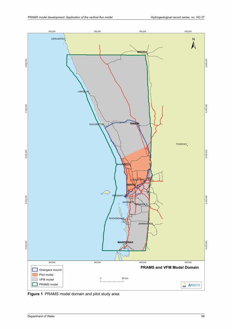
!
##
#
#
#
#
#
#
#
#
#
#
#
#
TOODYAY
WANNEROO
ARMADALE
LANCELIN
CERVANTES
FREMANTLE
GUILDFORD
ROCKINGHAM
JARRAHDALE
GUILDERTON
PERTH
MOORA
GINGIN
MANDURAH
JANDAKOT
300,000
300,000
350,000
350,000
400,000
400,000
450,000
450,000
6,40
0,00
0
6,40
0,00
0
6,45
0,00
0
6,45
0,00
0
6,50
0,00
0
6,50
0,00
0
6,55
0,00
0
6,55
0,00
0
6,60
0,00
0
6,60
0,00
0
±
PRAMS and VFM Model DomainGnangara mound
Pilot model
VFM model
PRAMS modelC O R P O R A T I O NWATER
0 25 km
Department of Water 59
PRAMS model development: Application of the vertical flux model Hydrogeological record series, no. HG 27
Figure 1 PRAMS model domain and pilot study area

60 Department of Water
Hydrogeological record series, no. HG 27 PRAMS model development: Application of the vertical flux model
VFM
MODFLOW
ClimateLanduses/vegetationSoil profile/ propertiesWatertable depthsTopography
HydrogeologySurfaceAquifer/layerHydraulic propertiesLithology/bore logs Monitoring boresWater levelDrainageBaseflow
AbstractionsPublicPrivateDomestic
Schematic of PRAMS Structure
Scen
ario
Man
ager
Figure 2 Schematic of PRAMS
Hydrological processes that control recharge on the Swan Coastal Plain
Gnangara Groundwater Mound
River
IndianOcean
Wetland
Dar
ling
Faul
t
Confining BedConfining Bed
Recharge
Infiltration
Interception
RedistributionPercolationDeep drainage
Transpiration Urban
Solar radiation
EVT
Recharge
EVT
Pasture
EVT
Runoff
Leakage
watertable
Confined aquifer
Superficialaquifer
Unsaturated zone
Rainfall
Saturated flow
EVT
Figure 3 Schematic showing hydrological processes that control recharge on the Swan Coastal Plain.

Department of Water 61
PRAMS model development: Application of the vertical flux model Hydrogeological record series, no. HG 27
Rainfall
Watertable Uns
atur
ated
zon
e
Interception
Evaporation
Transpiration
Transpiration
Redistribution
Infiltration
Deep drainage (recharge)
PercolationRoo
t zon
e
Litter
Soil
Runoff
Figure 4 Schematic of water balance in a soil column

#
!
##
#
#
#
#
#
#
#
#
#
#
#
22002000
1800
PERTH
MOORA
GINGIN
MANDURAH
700
800
900
600
500
1100 12
00
1000
1300
600
1300
300,000
300,000
350,000
350,000
400,000
400,000
450,000
450,000
6,40
0,00
0
6,40
0,00
0
6,45
0,00
0
6,45
0,00
0
6,50
0,00
0
6,50
0,00
0
6,55
0,00
0
6,55
0,00
0
6,60
0,00
0
6,60
0,00
0
±
Rainfall (mm)
500 - 600
601 - 800
801 - 1000
1001 - 1300
Annual PanEvap (mm)
Gnangara Mound
Landuse and climate
C O R P O R A T I O NWATER
0 25 km
62 Department of Water
Hydrogeological record series, no. HG 27 PRAMS model development: Application of the vertical flux model
Figure 5 Landuse and climate variability across the model domain

!
##
#
#
#
#
#
#
#
#
#
#
E
EE
E
E
TOODYAY
WANNEROO
ARMADALE
CERVANTES
FREMANTLE
GUILDFORD
ROCKINGHAM
GUILDERTON
MOORA
GINGIN
MANDURAH
9021PERTH AIRPORT
CHELSEA9006
LANCELIN9114
JARRAHDALE9023
JANDAKOT
PERTHPERTH REGIONAL
9034
300,000
300,000
350,000
350,000
400,000
400,000
450,000
450,000
6,40
0,00
0
6,40
0,00
0
6,45
0,00
0
6,45
0,00
0
6,50
0,00
0
6,50
0,00
0
6,55
0,00
0
6,55
0,00
0
6,60
0,00
0
6,60
0,00
0
±
VFM Climate ZonesE Climate stations
Gnangara mound
PRAMS model
Waves climate zones
1
2
3
4
5
C O R P O R A T I O NWATER
0 25 km
Department of Water 63
PRAMS model development: Application of the vertical flux model Hydrogeological record series, no. HG 27
Figure 6 Map for climate zones

64 Department of Water
Hydrogeological record series, no. HG 27 PRAMS model development: Application of the vertical flux model
Landuse compositions (2002)
Banksia woodland39%
Pine plantations 2%
Pasture48%
Urban10%
Market garden/parkland 0.3%
Lakes/wetlands 1%
Figure 7 Composition of primary landuse classifications (2002)

!
##
#
#
#
#
#
#
#
#
#
#
#
#
TOODYAY
WANNEROO
ARMADALE
LANCELIN
CERVANTES
FREMANTLE
GUILDFORD
ROCKINGHAM
JARRAHDALE
GUILDERTON
PERTH
MOORA
GINGIN
MANDURAH
JANDAKOT
300,000
300,000
350,000
350,000
400,000
400,000
450,000
450,000
6,40
0,00
0
6,40
0,00
0
6,45
0,00
0
6,45
0,00
0
6,50
0,00
0
6,50
0,00
0
6,55
0,00
0
6,55
0,00
0
6,60
0,00
0
6,60
0,00
0
±
VFM Landuse 2002
Gnangara mound
PRAMS model
Landuse 2002
Banksia low
Banksia medium
Banksia high
Pine low
Pine low-medium
Pine medium
Pine medium-high
Pine high
Urban residential
Urban Ind/Comm
Pasture
Parkland
Water
C O R P O R A T I O NWATER
0 25 km
Department of Water 65
PRAMS model development: Application of the vertical flux model Hydrogeological record series, no. HG 27
Figure 8 Landuse map for year 2002

!
##
#
#
#
#
#
#
#
#
#
#
#
#
TOODYAY
WANNEROO
ARMADALE
LANCELIN
CERVANTES
FREMANTLE
GUILDFORD
ROCKINGHAM
JARRAHDALE
GUILDERTON
PERTH
MOORA
GINGIN
MANDURAH
JANDAKOT
300,000
300,000
350,000
350,000
400,000
400,000
450,000
450,000
6,40
0,00
0
6,40
0,00
0
6,45
0,00
0
6,45
0,00
0
6,50
0,00
0
6,50
0,00
0
6,55
0,00
0
6,55
0,00
0
6,60
0,00
0
6,60
0,00
0
±
VFM classified soils(from surface geology)
Gnangara mound
PRAMS model
1 Quindalup soil
2 Spearwood soil
3 Bassendean soil
4 Guildford soil
5 Mesozoic soil
6 Lacustrine soilC O R P O R A T I O NWATER
0 25 km
66 Department of Water
Hydrogeological record series, no. HG 27 PRAMS model development: Application of the vertical flux model
Figure 9 Soil map
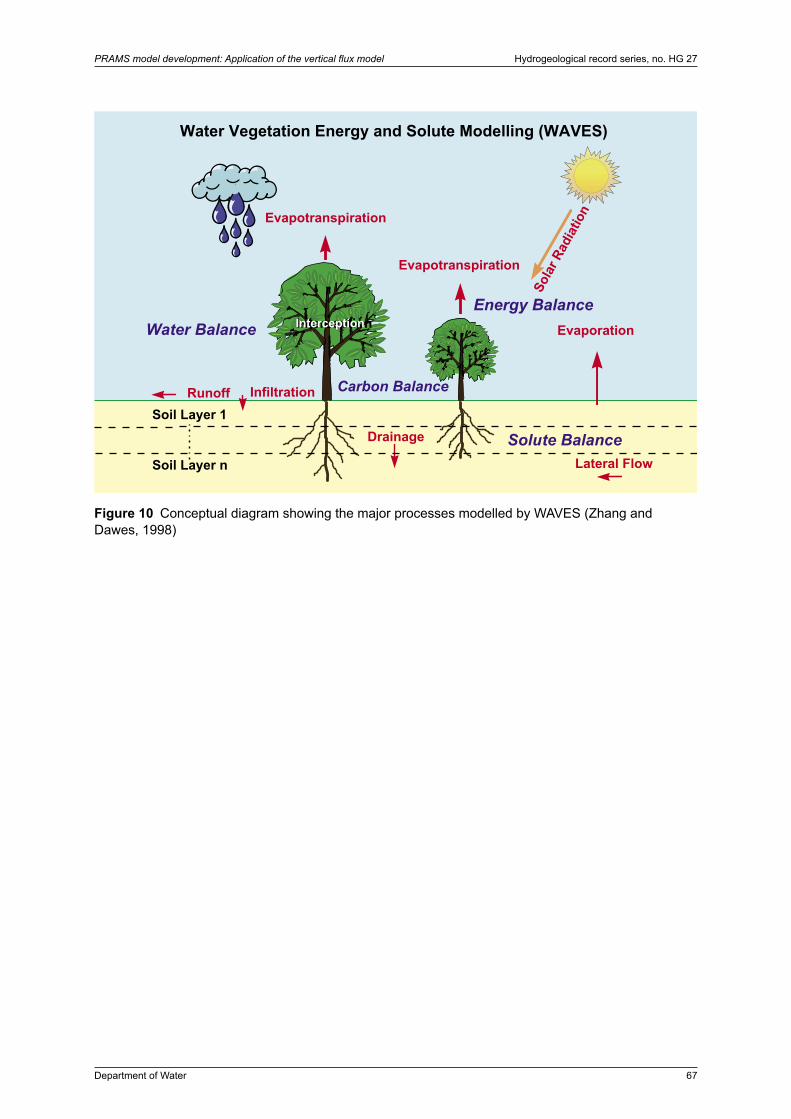
Department of Water 67
PRAMS model development: Application of the vertical flux model Hydrogeological record series, no. HG 27
Runoff Infiltration
Lateral FlowSoil Layer n
Soil Layer 1
Evaporation
Evapotranspiration
Drainage
Water Vegetation Energy and Solute Modelling (WAVES)
Evapotranspiration
Sola
r Rad
iatio
n
Solute Balance
Energy BalanceWater Balance InterceptionInterception
Carbon Balance
Figure 10 Conceptual diagram showing the major processes modelled by WAVES (Zhang and Dawes, 1998)

68 Department of Water
Hydrogeological record series, no. HG 27 PRAMS model development: Application of the vertical flux model
Bassendean topsoil A(Marked: Lab results; Soild: fitting b = 0.9 He = -0.12 m)
0.001
0.01
0.1
1
10
100
1000
(theta-theta_r)/(theta_s-theta_r)
Suct
ion
head
(m)
0 0.1 0.2 0.3 0.4 0.5 0.6 0.7 0.8 0.9 1.0
(a) Topsoil A
Bassendean topsoil B(Marked: Lab results; Solid: Fitting b = 0.8, He = -0.15 m)
0.001
0.01
0.1
1
10
100
1000
0 0.1 0.2 0.3 0.4 0.5 0.6 0.7 0.8 0.9 1.0
(theta-theta_r)/(theta_s-theta_r)
Suct
ion
head
(m)
(b) Topsoil B
Bassendean subsoil (drilling holes S2, S3 and PV3)(Marked: Lab results; Solid: fitting b = 0.9 He = -0.12 m)
0.01
0.01
0.1
1
10
100
1000
0 0.2 0.4 0.6 0.8 1.0
(theta-theta_r)/(theta_s-theta_r)
Suct
ion
head
(m)
(C) Subsoil C
Figure 11 Fitting water retention curve to soil data (Bassendean soil)
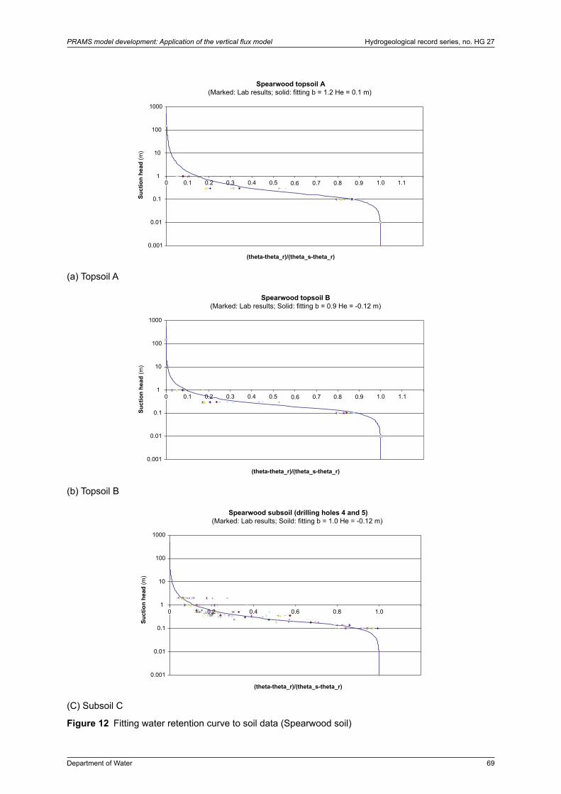
Department of Water 69
PRAMS model development: Application of the vertical flux model Hydrogeological record series, no. HG 27
0 0.2 0.30.1 0.4 0.5 0.8 0.90.70.6 1.0 1.1
Spearwood topsoil A(Marked: Lab results; solid: fitting b = 1.2 He = 0.1 m)
0.001
0.01
0.1
1
10
100
1000
(theta-theta_r)/(theta_s-theta_r)
Suct
ion
head
(m)
(a) Topsoil A
Spearwood topsoil B(Marked: Lab results; Solid: fitting b = 0.9 He = -0.12 m)
0.001
0.01
0.1
1
10
100
1000
(theta-theta_r)/(theta_s-theta_r)
Suct
ion
head
(m)
0 0.2 0.30.1 0.4 0.5 0.8 0.90.70.6 1.0 1.1
(b) Topsoil B
Spearwood subsoil (drilling holes 4 and 5)(Marked: Lab results; Soild: fitting b = 1.0 He = -0.12 m)
0.001
0.01
0.1
1
10
100
1000
0 0.2 0.4 0.6 0.8 1.0
(theta-theta_r)/(theta_s-theta_r)
Suct
ion
head
(m)
(C) Subsoil C
Figure 12 Fitting water retention curve to soil data (Spearwood soil)

70 Department of Water
Hydrogeological record series, no. HG 27 PRAMS model development: Application of the vertical flux model
K (theta) curve
0.001
0.01
0.1
1
10
100
1000
0 0.05 0.10 0.15 0.20 0.25 0.30 0.35
Theta
K (m
/d)
Insitu field measurementsFitting
Figure 13 Fitting unsaturated hydraulic conductivity curve to in situ measurement data (Bassendean soil)
Root Density Distribution for pines and banksia woodlands
0
0.005
0.010
0.015
0.020
0.025
0.030
0.035
0.040
0.045
0 2 4 6 8 10 12 14 16
Depth below ground level (m)
Den
sity
(kg/
m3 )
Banksia woodlandsPines
Figure 14 Root density distributions for pines and banksia woodlands
LAI for Annual Pasture
0
0.5
1.0
1.5
2.0
2.5
3.0
3.5
4.0
4.5
5.0
0 50 100 150 200 250 300 350 365
Day of year
LAI
Figure 15 LAI profile for annual pasture

Department of Water 71
PRAMS model development: Application of the vertical flux model Hydrogeological record series, no. HG 27
Ove
n dr
y fu
el w
eigh
t (t h
a-1)
Years since fire
Accumulation models for four fuel types in Banksia low woodlands near Perth, Western Australia? − Y = 7.36(1 − e−0.345x); − + − Y = 3.54(1 − e−0.327x); − × − Y = 2.45(1−−e−0.381x); − − Y = 1.38(1 − e−0.562x)
0
2
2 284 6 8 10 12 14 16 18 20 22 24 26
4
6
8
Total fuel
Live scrub fuel ≤ 4 mm diameter
Ground litter fuel
Aerated dead scrub fuel ≤ 6 mm diameter
Figure 16 Litter accumulations under banksia woodlands
Schematic of PRAMS 3.0
Multi-Layer Aquifer System(MODFLOW)
Unsaturated zone(VFM)
R
O
D
PEVT
RF
IR
P
IM
RO
Riv
ers
and
Oce
an
P = rainfallEVT = evapotranspirationIR = irrigated water
explicitly modelled)RF = return flowP = pumpingRO = runoff (not explicitly
D = drainageO = outflow to oceanR = recharge/uptakePW = public water supply
PW
IM = imported water (not
modelled)
Figure 17 Schematic of PRAMS showing water balance components considered in the model

72 Department of Water
Hydrogeological record series, no. HG 27 PRAMS model development: Application of the vertical flux model
Recharge under different landuse clasess [climate zone 4 (Perth region), Bassendean soil]
-50%
-40%
-30%
-20%
-10%
0%
10%
20%
30%
40%
50%
60%
70%
0 2 4 6 8 10 12 14
Watertable depth (m)
Rec
harg
e as
% o
f rai
nfal
l
Pasture (3) Banksia low (2)Banksia medium (22) Banksia high (1)Pine low (8) Pine low to medium (18)Pine medium (7) Pine medium to high (17)Pine high (6)
Figure 18 Estimated recharge for various landuse by WAVES (Bassendean soil)
Water balance components under different landuse classes[Climate zone: 4 (Perth region); Bassendean soil, large watertable depth]
0%
10%
20%
30%
40%
50%
60%
70%
80%
(6)Pine
(3)Pasture
Landuse class
% o
f rai
nfal
l
Interception lossLitter interception/soil evaporationTranspirationDeep drainage (recharge)
(2)Banksia
(22)Banksia
(1)Banksia
(8)Pine
(18)Pine
(7)Pine
(17)Pine
Figure 19 Water balance components for pasture, native woodlands and pines (watertable depth greater than 15 m)

Department of Water 73
PRAMS model development: Application of the vertical flux model Hydrogeological record series, no. HG 27
Recharge under different landuse clasess [climate zone 4 (Perth region), Spearwood soil]
-50%
-40%
-30%
-20%
-10%
0%
10%
20%
30%
40%
50%
60%
70%
0 2 4 8 106 12 14
Rec
harg
e as
% o
f rai
nfal
l
Pasture (3) Banksia low (2)Banksia medium (22) Banksia high (1)Pine low (8) Pine low to medium (18)Pine medium (7) Pine medium to high (17)Pine high (6)
Watertable depth (m)
Figure 20 Estimated recharge for various landuse by WAVES (Spearwood soil)
Recharge under different climate(Bassendean soil; watertable depth >15 m)
0
100
200
300
400
500
600
700
500 600 700 800 900 1000 1100 1200
Averaged annual rainfall (mm)
Ann
ual r
echa
rge
(mm
)
Pasture (3)
Banksia low (2)
Banksia medium (22)
Banksia high (1)
Figure 21 Recharge under different climate regimes (Bassendean soil)
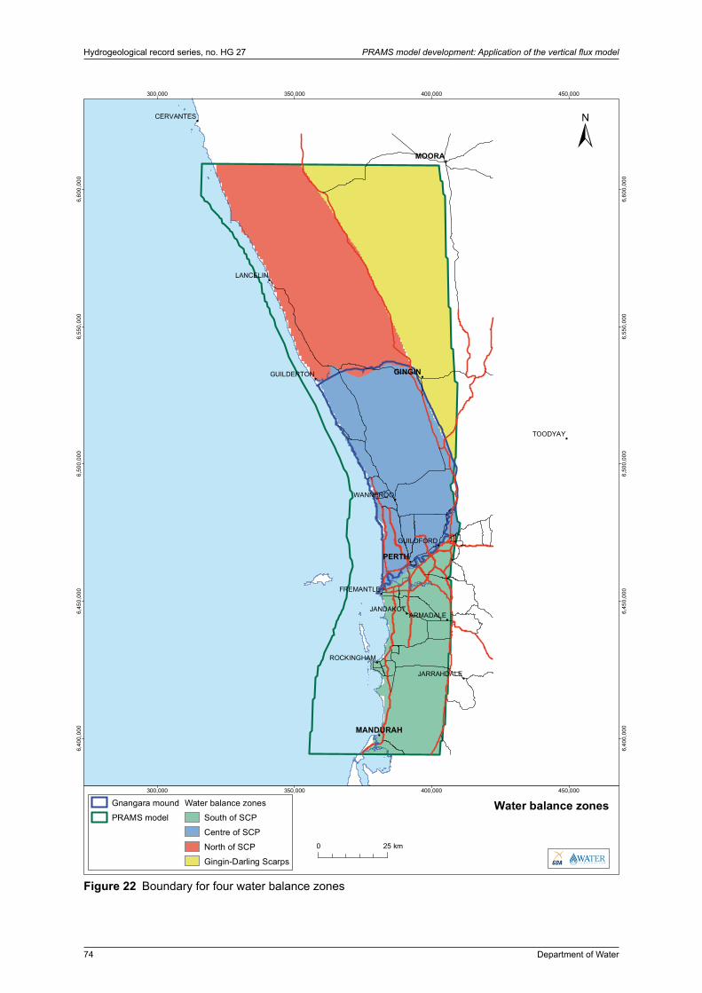
!
##
#
#
#
#
#
#
#
#
#
#
#
#
TOODYAY
WANNEROO
ARMADALE
LANCELIN
CERVANTES
FREMANTLE
GUILDFORD
ROCKINGHAM
JARRAHDALE
GUILDERTON
PERTH
MOORA
GINGIN
MANDURAH
JANDAKOT
300,000
300,000
350,000
350,000
400,000
400,000
450,000
450,000
6,40
0,00
0
6,40
0,00
0
6,45
0,00
0
6,45
0,00
0
6,50
0,00
0
6,50
0,00
0
6,55
0,00
0
6,55
0,00
0
6,60
0,00
0
6,60
0,00
0
±
Water balance zonesGnangara mound
PRAMS model
Water balance zones
South of SCP
Centre of SCP
North of SCP
Gingin-Darling Scarps C O R P O R A T I O NWATER
0 25 km
74 Department of Water
Hydrogeological record series, no. HG 27 PRAMS model development: Application of the vertical flux model
Figure 22 Boundary for four water balance zones

Department of Water 75
PRAMS model development: Application of the vertical flux model Hydrogeological record series, no. HG 27
Annual recharge (mm) for four areas
0
50
100
150
200
250
300
19861984 1988 1990 1992 1994 1996 1998 2000 2002 2004
Year
Rec
harg
e (m
m/a
)
South Centre North Gingin-Darling scarp
Figure 23 Annual recharge (mm) for four zones for period 1985–2004
South Centre North Gingin-Darling scarp
19861984 1988 1990 1992 1994 1996 1998 2000 2002 2004
Year
Annual recharge (GL) for four areas
0
100
200
300
400
500
600
Rec
harg
e (G
L/a)
Figure 24 Annual recharge (GL) for period 1985–2004
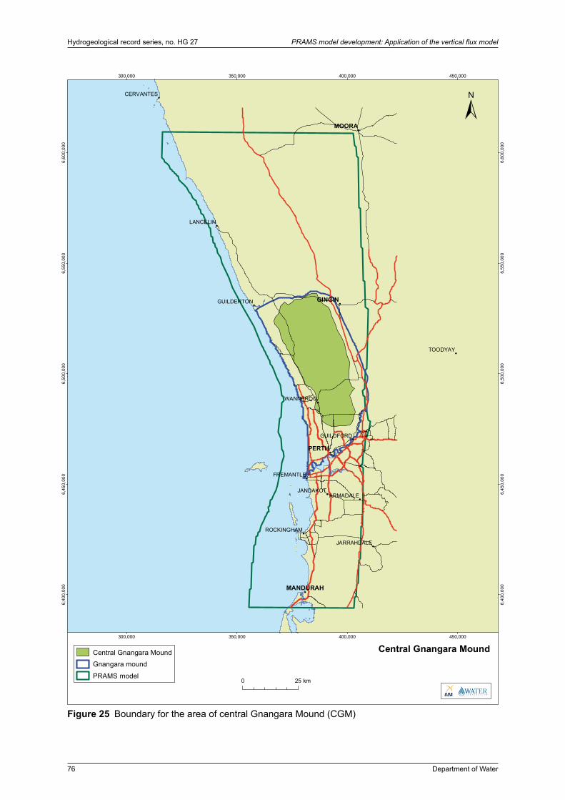
!
##
#
#
#
#
#
#
#
#
#
#
#
#
TOODYAY
WANNEROO
ARMADALE
LANCELIN
CERVANTES
FREMANTLE
GUILDFORD
ROCKINGHAM
JARRAHDALE
GUILDERTON
PERTH
MOORA
GINGIN
MANDURAH
JANDAKOT
300,000
300,000
350,000
350,000
400,000
400,000
450,000
450,000
6,40
0,00
0
6,40
0,00
0
6,45
0,00
0
6,45
0,00
0
6,50
0,00
0
6,50
0,00
0
6,55
0,00
0
6,55
0,00
0
6,60
0,00
0
6,60
0,00
0
±
Central Gnangara MoundCentral Gnangara Mound
Gnangara mound
PRAMS model
C O R P O R A T I O NWATER
0 25 km
76 Department of Water
Hydrogeological record series, no. HG 27 PRAMS model development: Application of the vertical flux model
Figure 25 Boundary for the area of central Gnangara Mound (CGM)

Department of Water 77
PRAMS model development: Application of the vertical flux model Hydrogeological record series, no. HG 27
Annual recharge for the central area of Gnangara Mound
0
50
100
150
200
250
300
350
Rec
harg
e (G
L/a)
0
200
400
600
800
1000
1200
1400
Ann
ual r
ainf
all (
mm
)
Annual rechargeAveraged recharge for 1985–1997 = 206 GL/aAveraged recharge for 1997–2003 = 155 GL/aAnnual rainfall
19861984 1988 1990 1992 1994 1996 1998 2000 2002 2004
Year
Figure 26 Annual recharge (GL) for the CGM for period 1985–2004
Annual recharge for the central area of Gnangara Mound
0
50
100
150
200
250
300
Rec
harg
e (m
m/a
)
0
200
400
600
800
1000
1200
Ann
ual r
ainf
all (
mm
)
Annual recharge for other landuseAnnual recharge for pinesAnnual rainfall
19861984 1988 1990 1992 1994 1996 1998 2000 2002 2004
Year
Figure 27 Annual recharge (mm) for pines and other landuse in CGM area
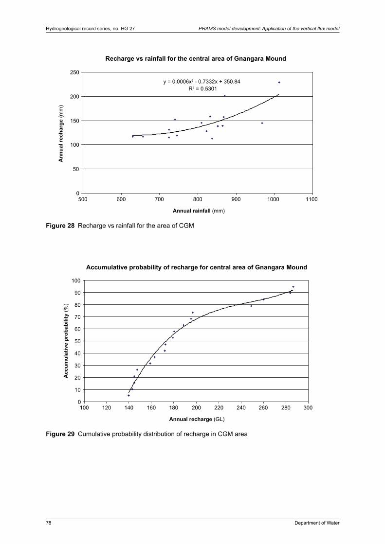
78 Department of Water
Hydrogeological record series, no. HG 27 PRAMS model development: Application of the vertical flux model
Recharge vs rainfall for the central area of Gnangara Mound
y = 0.0006x2 - 0.7332x + 350.84R2 = 0.5301
0
50
100
150
200
250
500 600 700 800 900 1000 1100
Annual rainfall (mm)
Ann
ual r
echa
rge
(mm
)
Figure 28 Recharge vs rainfall for the area of CGM
Accumulative probability of recharge for central area of Gnangara Mound
0
10
20
30
40
50
60
70
80
90
100
100 120 140 160 180 200 220 240 260 280 300
Annual recharge (GL)
Acc
umul
ativ
e pr
obab
ility
(%)
Figure 29 Cumulative probability distribution of recharge in CGM area

C O R P O R A T I O NWATER
0 25 km
!
##
#
#
#
#
#
#
#
#
#
#
#
#
147
89
115
0
55
56
46
65
0
155
150
140
147
109
125
177
120
136
90
121
0
194
331
201
117
332
206
0
148
23
80
356
-53
0
113
127
265
115
11971
208
142
282
-33
0
161
103
329
228
0
41
12
306
144
157
-50
24
209
226
53
85
238
30
206
383
257
223
293
212
315302
318
384
152
177
-48
-157
201
341
368
334
303
371318
232
22
390318
273195349
304
157
105
262
282
250
354
188184
219
175
389
372 117
394329
260
325
318
303
TOODYAY
ARMADALE
LANCELIN
CERVANTES
ROCKINGHAM
JARRAHDALE
GUILDERTON
MOORA
GINGIN
MANDURAH
WANNEROO
JANDAKOT
FREMANTLE
GUILDFORD
PERTH
300,000
300,000
350,000
350,000
400,000
400,000
450,000
450,000
6,40
0,00
0
6,40
0,00
0
6,45
0,00
0
6,45
0,00
0
6,50
0,00
0
6,50
0,00
0
6,55
0,00
0
6,55
0,00
0
6,60
0,00
0
6,60
0,00
0
±
Recharge annual average1985-2003 (mm/yr)Gnangara mound
PRAMS model
1985-2003 (mm/yr)
< 0
0 - 50
50 - 100
100 - 150
150 - 200
200 - 250
250 - 400
Department of Water 79
PRAMS model development: Application of the vertical flux model Hydrogeological record series, no. HG 27
Figure 30 Recharge map showing averaged annual recharge (mm) for 1985–2003

C O R P O R A T I O NWATER
0 25 km
!
##
#
#
#
#
#
#
#
#
#
#
#
#
126
77
120
1
50
92
36
97
81
28
47
83
0
126
124
104
123
144
110
55
0
176
304
152
10780
303
201
0
146
25
6991
322
-44
0
103
131
237
11267
197
113
272
-35
0
136
311
215
0
37
12
272
130
151
-44
39
211
208
49
80
230
16
182
354
197
191
271
211
283293
277
367
141
79
153
-56
-213
176
301
335
315
274
350277
202
23
367284
254195312
282
151
216
236
351
224
319
188145
208
154
351
347 108
367326
304
284
268
TOODYAY
ARMADALE
LANCELIN
CERVANTES
ROCKINGHAM
JARRAHDALE
GUILDERTON
MOORA
GINGIN
MANDURAH
WANNEROO
JANDAKOT
FREMANTLE
GUILDFORD
PERTH
300,000
300,000
350,000
350,000
400,000
400,000
450,000
450,000
6,40
0,00
0
6,40
0,00
0
6,45
0,00
0
6,45
0,00
0
6,50
0,00
0
6,50
0,00
0
6,55
0,00
0
6,55
0,00
0
6,60
0,00
0
6,60
0,00
0
±
Recharge annual average1997-2003 (mm/yr)Gnangara mound
PRAMS model
1997-2003 (mm/yr)
< 0
0 - 50
50 - 100
100 - 150
150 - 200
200 - 250
25 - 370
80 Department of Water
Hydrogeological record series, no. HG 27 PRAMS model development: Application of the vertical flux model
Figure 31 Recharge map showing averaged annual recharge (mm) under drier climate (1997–2003)
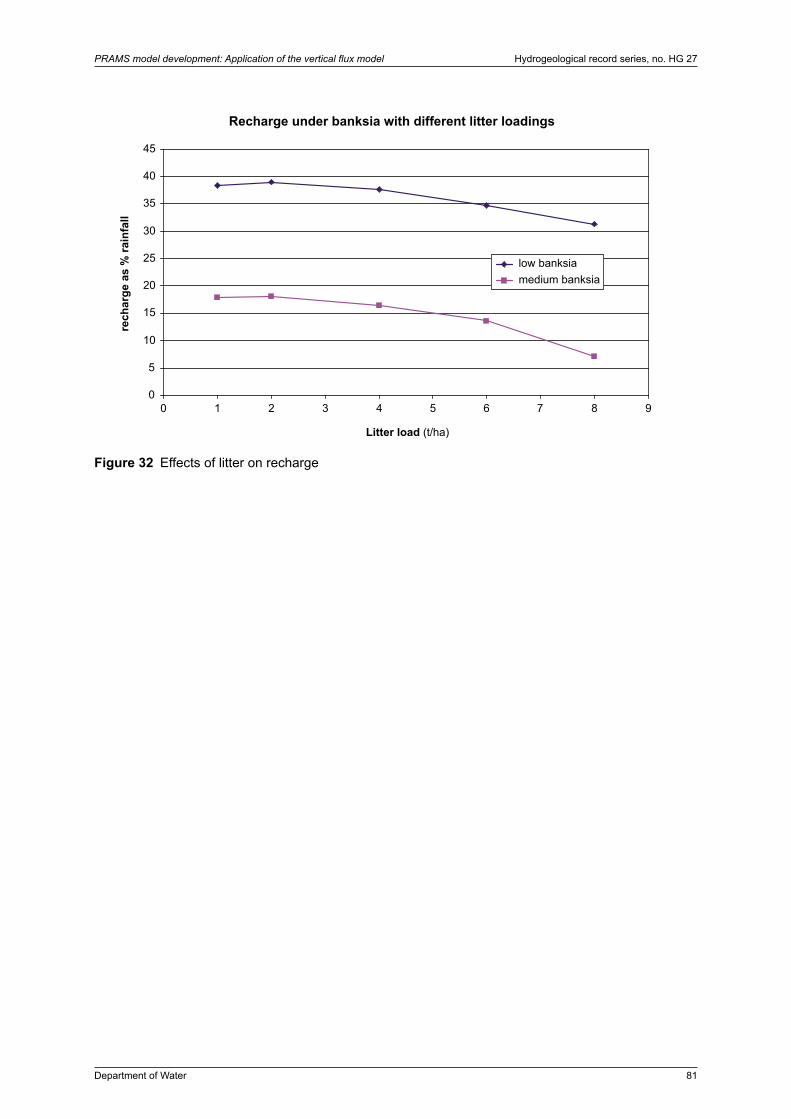
Department of Water 81
PRAMS model development: Application of the vertical flux model Hydrogeological record series, no. HG 27
Recharge under banksia with different litter loadings
0
5
10
15
20
25
30
35
40
45
0 1 2 3 4 5 6 7 8 9
Litter load (t/ha)
rech
arge
as
% ra
infa
ll
low banksiamedium banksia
Figure 32 Effects of litter on recharge

82 Department of Water
Hydrogeological record series, no. HG 27 PRAMS model development: Application of the vertical flux model

Department of Water 83
PRAMS model development: Application of the vertical flux model Hydrogeological record series, no. HG 27
Appendix 1 Dataset for PRAMS 3.0
This appendix lists the files required to run PRAMS 3.0. All file names except Vfmm.def and Vfmm.rru are indicative only and can be changed to any other names. A typical example of the VFM manager files is also given where appropriate. Details of WAVES files and their structures can be found in the WAVES user guides (Zhang and Dawes, 1998) or VFM user manual (Barr et al., 2003).
Table I – 1 List of input files for PRAMS model
MODFLOW files VFM Manager files WAVES files
modflow.bf vfmm.def Climate files
modflow.in vfmm.rru Chelsea.clm
bas.dat RRU attribute files Lancelin.clm
bcf.dat vfmlanduse.lu Perthairport.clm
wel.dat vfmwater.wt Perthregion.clm
rch.dat* vfmsoil.sp Jarrahdale.clm
oc.dat vfmclimate.cl Vegetation files
pcg2.dat Landuse files pine_MR12.veg
drn.dat banksia_H.lu pine_expMax12.rot
hfb1.dat banksia_M.lu banksia4.veg
pramsVFM.dat banksia_L.lu banksialog10.rot
Pasture.lu pasture.veg
pine_H.lu Pasture.rot
pine_M17.lu Pasture_3.lai
pine_M7.lu Soil table and node file
pine_L18.lu bassendean.nod
pine_L8.lu bassendeanA_cp.tab
lakes_pl.lu bassendeanB_cp.tab
urban_resid.lu bassendeanC_k10_cp.tab
urban_com.lu spearwood.nod
marketgarden.lu spearwoodA.tab
Soil profile files spearwoodB.tab
quindalup.sp spearwoodC_k5_cp.dat
spearwood.sp quindalup.nod
bassendean.sp quindalupA_cp.tab
guildford.sp quindalupB_cp.tab
mesozoic.sp guildford.nod
lacustrine.sp guildford_bw01.tab
mesozoic.nod
mesozoicA_cp.tab
mesozoicB_cp.tab
lacustrine.nod
lacustrineA_k01_cp.tab
lacustrineB_cp.tab
* Rch.dat used to model the abstraction by domestic garden bores

84 Department of Water
Hydrogeological record series, no. HG 27 PRAMS model development: Application of the vertical flux model
Table I – 2 An example VFM Manager defaults file (‘vfmm.def’)
# Defaults file for the VFM Manager Package for MODFLOW
# Simulation Options
false : (DOSXP) Solute transport
false : (DOFLOOD) Surface flooding
false : (GROWON) Growth
# WAVES Simulation Parameters
-32.00 : (XLAT) Latitude
0.00 : (XSLP) Slope
0.00 : (XASP) Aspect
0.0001 : (CPPT) Concentration in precipitation
0.00001 : (CGW) Concentration in groundwater
0.000 : (CFLD) Concentration in flood water
1.0 : (RELAX) Relaxation factor
0 : (NLAYG) Number of layers for growth
0.99 : (SAT_CUTOFF) Saturation at which roots die
# VFM Manager simulation parameters
31/12/1979 : (DAY0) Day prior to start of MODFLOW simulation
false : (USESTARTFILE) Use start file for initialisation
730 : (DAYSPRESIM) Initialisation time (days) for RRUs
4 : (NDBLWWT) Nodes in WAVES simulation below watertable
0.5 : (CAPILLZONE) Thickness of capillary zone
false : (TRUNCRMAX) Truncate maximum root depth at watertable
0.05 : (WTLAKEINDIC) Watertable depth to use lake model
PIECEWISE_LINEAR : (WVSWTMODEL) Lake model
LAKE_PL.lu : (WTLAKEFL) Model data
# Output options
true : (DOLOGFILE) VFM Manager log file
false : (DOWVLOGFILE) WAVES log file
false : (DOSTARTFILE) Start file
false : (DOFINALFILE) Finish file
false : (DOHYFILE) Hydraulic heads file
false : (DOSLFILE) Solute concentration file
false : (DODPFILE) Dump files (WRD debug)
false : (DOVGFILE) Vegetation file(s)
false : (DORCFILE) Root carbon file(s)
false : (DOFLFILE) Flux file
false : (DOSKFILE) Sink file

Department of Water 85
PRAMS model development: Application of the vertical flux model Hydrogeological record series, no. HG 27
Table I – 3 List of attribute filenames file (‘vfmm.rru’)
# vfmm.rru List of files containing attribute codes for the VFMMVFMwater.wt : Watertable attribute fileVFMlanduse.lu : Landuse attribute fileVFMclimate.cl : Climate attribute fileVFMsoil.sp : Soil profile attribute filevfmm.log : Log file for output
Table I – 4 Example of climate attribute file
# VFMclimate.cl : List of data to construct individual climate zones5 : Number of climates# Climate 1 : North of Gingin (dry and hot)1 : ID for this zone on climate mapChelsea.clm : Climate data file# Climate 2 : Lancelin2 : ID for this zone on climate mapLancelin.clm : Climate data file# Climate 3 : Perth airport3 : ID for this zone on climate map PerthAirport.clm : Climate data file# Climate 4 : Perth region (Mt Lawly)4 : ID for this zone on climate map PerthRegion.clm : Climate data file# Climate 5 : Jarrahdale5 : ID for this zone on climate mapJarrahdale.clm : Climate data file
Table I – 5 Example of a soil profile attribute file
# VFMSOIL.SP List of all soil profile zones used in WAVES6 : Number of soil profiles # Soil Profile 1 : Quindalup soil1 : Soil profile indexquindalup.sp : Soil profile data file# Soil Profile 2 : Spearwood soil2 : Soil profile index Spearwood.sp : Soil profile data file# Soil Profile 3 : Bassendean soil 3 : Soil profile index Bassendean.sp : Soil profile data file# Soil Profile 4 : Guildford soil4 : Soil profile indexGuildford.sp : Soil profile data file# Soil Profile 5 : Mesozoic soil 5 : Soil profile index Mesozoic.sp : Soil profile data file# Soil Profile 6 : Lacustrine soil6 : Soil profile indexLacustrine.sp : Soil profile data file
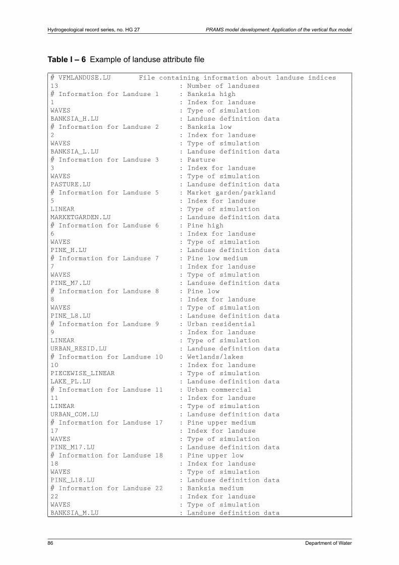
86 Department of Water
Hydrogeological record series, no. HG 27 PRAMS model development: Application of the vertical flux model
Table I – 6 Example of landuse attribute file
# VFMLANDUSE.LU File containing information about landuse indices13 : Number of landuses# Information for Landuse 1 : Banksia high1 : Index for landuse WAVES : Type of simulation BANKSIA_H.LU : Landuse definition data# Information for Landuse 2 : Banksia low2 : Index for landuseWAVES : Type of simulation BANKSIA_L.LU : Landuse definition data# Information for Landuse 3 : Pasture3 : Index for landuseWAVES : Type of simulation PASTURE.LU : Landuse definition data# Information for Landuse 5 : Market garden/parkland5 : Index for landuseLINEAR : Type of simulationMARKETGARDEN.LU : Landuse definition data# Information for Landuse 6 : Pine high6 : Index for landuseWAVES : Type of simulation PINE_H.LU : Landuse definition data# Information for Landuse 7 : Pine low medium7 : Index for landuseWAVES : Type of simulation PINE_M7.LU : Landuse definition data# Information for Landuse 8 : Pine low8 : Index for landuseWAVES : Type of simulation PINE_L8.LU : Landuse definition data# Information for Landuse 9 : Urban residential9 : Index for landuse LINEAR : Type of simulation URBAN_RESID.LU : Landuse definition data# Information for Landuse 10 : Wetlands/lakes10 : Index for landusePIECEWISE_LINEAR : Type of simulation LAKE_PL.LU : Landuse definition data# Information for Landuse 11 : Urban commercial11 : Index for landuseLINEAR : Type of simulation URBAN_COM.LU : Landuse definition data# Information for Landuse 17 : Pine upper medium17 : Index for landuseWAVES : Type of simulation PINE_M17.LU : Landuse definition data# Information for Landuse 18 : Pine upper low18 : Index for landuseWAVES : Type of simulation PINE_L18.LU : Landuse definition data# Information for Landuse 22 : Banksia medium22 : Index for landuseWAVES : Type of simulation BANKSIA_M.LU : Landuse definition data

Department of Water 87
PRAMS model development: Application of the vertical flux model Hydrogeological record series, no. HG 27
Table I – 7 Example of a watertable attribute file
# VFMwater.wt List of all watertable depths available for WAVES
8 : Number of watertable depths
0.1 : Smallest watertable depth
1.0
2.0
4.0
6.0
10.0
15.0
50.0 : Largest watertable depth
Table I – 8 Example of a WAVES landuse definition file (Banksia_H.LU)
# Banksia_H.LU Banksia high desnity landuse file
n : Consider an understorey? [y/n]
Banksia4.veg : Vegetation parameter file
n : Provide updates for leaf area index from a file?
0.21 : Constant leaf carbon value (6*0.21=1.26)
0.2000 : Initial leaf/stem ratio
0.2500 : Initial litter pool (2.5 t/ha)
0.2000 : Normalised N(utrient) value
BanksiaLog10.rot : Root carbon distribution file
Table I – 9 Example of a WAVES landuse definition file (Pasture.LU)
# Pasture.LU Pasture landuse file
n : Consider an understorey? [y/n]
pasture.veg : Vegetation parameter file
y : Whether to update LAI [y/n]
pasture_3.lai : Time-varying LAI file
0.00000 : Leaf carbon value [0-1]
1.00000 : Initial leaf/stem ratio [0-1]
0.00000 : Initial litter pool [0-1]
0.20000 : Normalised nutrient value [0-1]
pasture.rot : Root carbon distribution file
Table I – 10 Example of a LINEAR landuse file
# urban_resid.lu Data for linear model representing urban landuse
0.62 : Multiplier for rainfall (α) 0.05 : Multiplier for evaporation (β)

88 Department of Water
Hydrogeological record series, no. HG 27 PRAMS model development: Application of the vertical flux model
Table I – 11 Example of a soil profile description file
# Spearwood.sp Soil profile information for Spearwood soil
# Soil profile information
SpearwoodA_cp.tab : Soil table for top soil horizon A
SpearwoodB_cp.tab : Soil table for top soil horizon B
SpearwoodC_k5_cp.tab : Soil table for top soil horizon C
n : Consider an understorey? [y/n]
Spearwood.nod : Node file to define the soil layers

!
##
#
#
#
#
#
#
#
#
#
#
#
#
TOODYAY
WANNEROO
ARMADALE
LANCELIN
CERVANTES
FREMANTLE
GUILDFORD
ROCKINGHAM
JARRAHDALE
GUILDERTON
PERTH
MOORA
GINGIN
MANDURAH
JANDAKOT
300,000
300,000
350,000
350,000
400,000
400,000
450,000
450,000
6,40
0,00
0
6,40
0,00
0
6,45
0,00
0
6,45
0,00
0
6,50
0,00
0
6,50
0,00
0
6,55
0,00
0
6,55
0,00
0
6,60
0,00
0
6,60
0,00
0
±
VFM Landuse 1985
Gnangara mound
PRAMS model
Landuse 1985Banksia low
Banksia medium
Banksia high
Pine low
Pine low-medium
Pine medium
Pine medium-high
Pine high
Urban residential
Urban Ind/Comm
Pasture
Parkland
Water
C O R P O R A T I O NWATER
0 25 km
Department of Water 89
PRAMS model development: Application of the vertical flux model Hydrogeological record series, no. HG 27
Appendix 2 Historical landuse maps
Figure II – 1 Landuse map (1985)

!
##
#
#
#
#
#
#
#
#
#
#
#
#
TOODYAY
WANNEROO
ARMADALE
LANCELIN
CERVANTES
FREMANTLE
GUILDFORD
ROCKINGHAM
JARRAHDALE
GUILDERTON
PERTH
MOORA
GINGIN
MANDURAH
JANDAKOT
300,000
300,000
350,000
350,000
400,000
400,000
450,000
450,000
6,40
0,00
0
6,40
0,00
0
6,45
0,00
0
6,45
0,00
0
6,50
0,00
0
6,50
0,00
0
6,55
0,00
0
6,55
0,00
0
6,60
0,00
0
6,60
0,00
0
±
VFM Landuse 1988
Gnangara mound
PRAMS model
Landuse 1988Banksia low
Banksia medium
Banksia high
Pine low
Pine low-medium
Pine medium
Pine medium-high
Pine high
Urban residential
Urban Ind/Comm
Pasture
Parkland
Water
C O R P O R A T I O NWATER
0 25 km
90 Department of Water
Hydrogeological record series, no. HG 27 PRAMS model development: Application of the vertical flux model
Figure II – 2 Landuse map (1988)

!
##
#
#
#
#
#
#
#
#
#
#
#
#
TOODYAY
WANNEROO
ARMADALE
LANCELIN
CERVANTES
FREMANTLE
GUILDFORD
ROCKINGHAM
JARRAHDALE
GUILDERTON
PERTH
MOORA
GINGIN
MANDURAH
JANDAKOT
300,000
300,000
350,000
350,000
400,000
400,000
450,000
450,000
6,40
0,00
0
6,40
0,00
0
6,45
0,00
0
6,45
0,00
0
6,50
0,00
0
6,50
0,00
0
6,55
0,00
0
6,55
0,00
0
6,60
0,00
0
6,60
0,00
0
±
VFM Landuse 1990
Gnangara mound
PRAMS model
Landuse 1990Banksia low
Banksia medium
Banksia high
Pine low
Pine low-medium
Pine medium
Pine medium-high
Pine high
Urban residential
Urban Ind/Comm
Pasture
Parkland
Water
C O R P O R A T I O NWATER
0 25 km
Department of Water 91
PRAMS model development: Application of the vertical flux model Hydrogeological record series, no. HG 27
Figure II – 3 Landuse map (1990)
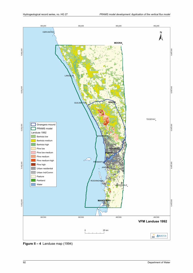
!
##
#
#
#
#
#
#
#
#
#
#
#
#
TOODYAY
WANNEROO
ARMADALE
LANCELIN
CERVANTES
FREMANTLE
GUILDFORD
ROCKINGHAM
JARRAHDALE
GUILDERTON
PERTH
MOORA
GINGIN
MANDURAH
JANDAKOT
300,000
300,000
350,000
350,000
400,000
400,000
450,000
450,000
6,40
0,00
0
6,40
0,00
0
6,45
0,00
0
6,45
0,00
0
6,50
0,00
0
6,50
0,00
0
6,55
0,00
0
6,55
0,00
0
6,60
0,00
0
6,60
0,00
0
±
VFM Landuse 1992
Gnangara mound
PRAMS model
Landuse 1992Banksia low
Banksia medium
Banksia high
Pine low
Pine low-medium
Pine medium
Pine medium-high
Pine high
Urban residential
Urban Ind/Comm
Pasture
Parkland
Water
C O R P O R A T I O NWATER
0 25 km
92 Department of Water
Hydrogeological record series, no. HG 27 PRAMS model development: Application of the vertical flux model
Figure II – 4 Landuse map (1994)

!
##
#
#
#
#
#
#
#
#
#
#
#
#
TOODYAY
WANNEROO
ARMADALE
LANCELIN
CERVANTES
FREMANTLE
GUILDFORD
ROCKINGHAM
JARRAHDALE
GUILDERTON
PERTH
MOORA
GINGIN
MANDURAH
JANDAKOT
300,000
300,000
350,000
350,000
400,000
400,000
450,000
450,000
6,40
0,00
0
6,40
0,00
0
6,45
0,00
0
6,45
0,00
0
6,50
0,00
0
6,50
0,00
0
6,55
0,00
0
6,55
0,00
0
6,60
0,00
0
6,60
0,00
0
±
VFM Landuse 1996
Gnangara mound
PRAMS model
Landuse 1996Banksia low
Banksia medium
Banksia high
Pine low
Pine low-medium
Pine medium
Pine medium-high
Pine high
Urban residential
Urban Ind/Comm
Pasture
Parkland
Water
C O R P O R A T I O NWATER
0 25 km
Department of Water 93
PRAMS model development: Application of the vertical flux model Hydrogeological record series, no. HG 27
Figure II – 5 Landuse map (1996)

!
##
#
#
#
#
#
#
#
#
#
#
#
#
TOODYAY
WANNEROO
ARMADALE
LANCELIN
CERVANTES
FREMANTLE
GUILDFORD
ROCKINGHAM
JARRAHDALE
GUILDERTON
PERTH
MOORA
GINGIN
MANDURAH
JANDAKOT
300,000
300,000
350,000
350,000
400,000
400,000
450,000
450,000
6,40
0,00
0
6,40
0,00
0
6,45
0,00
0
6,45
0,00
0
6,50
0,00
0
6,50
0,00
0
6,55
0,00
0
6,55
0,00
0
6,60
0,00
0
6,60
0,00
0
±
VFM Landuse 1998
Gnangara mound
PRAMS model
Landuse 1998Banksia low
Banksia medium
Banksia high
Pine low
Pine low-medium
Pine medium
Pine medium-high
Pine high
Urban residential
Urban Ind/Comm
Pasture
Parkland
Water
C O R P O R A T I O NWATER
0 25 km
94 Department of Water
Hydrogeological record series, no. HG 27 PRAMS model development: Application of the vertical flux model
Figure II – 6 Landuse map (1998)

!
##
#
#
#
#
#
#
#
#
#
#
#
#
TOODYAY
WANNEROO
ARMADALE
LANCELIN
CERVANTES
FREMANTLE
GUILDFORD
ROCKINGHAM
JARRAHDALE
GUILDERTON
PERTH
MOORA
GINGIN
MANDURAH
JANDAKOT
300,000
300,000
350,000
350,000
400,000
400,000
450,000
450,000
6,40
0,00
0
6,40
0,00
0
6,45
0,00
0
6,45
0,00
0
6,50
0,00
0
6,50
0,00
0
6,55
0,00
0
6,55
0,00
0
6,60
0,00
0
6,60
0,00
0
±
VFM Landuse 2000
Gnangara mound
PRAMS model
Landuse 2000Banksia low
Banksia medium
Banksia high
Pine low
Pine low-medium
Pine medium
Pine medium-high
Pine high
Urban residential
Urban Ind/Comm
Pasture
Parkland
Water
C O R P O R A T I O NWATER
0 25 km
Department of Water 95
PRAMS model development: Application of the vertical flux model Hydrogeological record series, no. HG 27
Figure II – 7 Landuse map (2000)
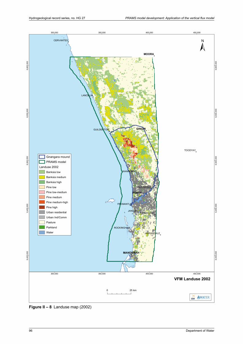
!
##
#
#
#
#
#
#
#
#
#
#
#
#
TOODYAY
WANNEROO
ARMADALE
LANCELIN
CERVANTES
FREMANTLE
GUILDFORD
ROCKINGHAM
JARRAHDALE
GUILDERTON
PERTH
MOORA
GINGIN
MANDURAH
JANDAKOT
300,000
300,000
350,000
350,000
400,000
400,000
450,000
450,000
6,40
0,00
0
6,40
0,00
0
6,45
0,00
0
6,45
0,00
0
6,50
0,00
0
6,50
0,00
0
6,55
0,00
0
6,55
0,00
0
6,60
0,00
0
6,60
0,00
0
±
VFM Landuse 2002
Gnangara mound
PRAMS model
Landuse 2002
Banksia low
Banksia medium
Banksia high
Pine low
Pine low-medium
Pine medium
Pine medium-high
Pine high
Urban residential
Urban Ind/Comm
Pasture
Parkland
Water
C O R P O R A T I O NWATER
0 25 km
96 Department of Water
Hydrogeological record series, no. HG 27 PRAMS model development: Application of the vertical flux model
Figure II – 8 Landuse map (2002)
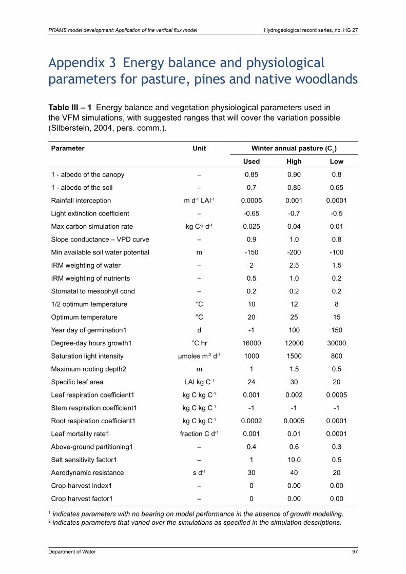
Department of Water 97
PRAMS model development: Application of the vertical flux model Hydrogeological record series, no. HG 27
Appendix 3 Energy balance and physiological parameters for pasture, pines and native woodlands
Table III – 1 Energy balance and vegetation physiological parameters used in the VFM simulations, with suggested ranges that will cover the variation possible (Silberstein, 2004, pers. comm.).
Parameter Unit Winter annual pasture (C3)
Used High Low
1 - albedo of the canopy
1 - albedo of the soil
Rainfall interception
Light extinction coefficient
Max carbon simulation rate
Slope conductance – VPD curve
Min available soil water potential
IRM weighting of water
IRM weighting of nutrients
Stomatal to mesophyll cond
1/2 optimum temperature
Optimum temperature
Year day of germination1
Degree-day hours growth1
Saturation light intensity
Maximum rooting depth2
Specific leaf area
Leaf respiration coefficient1
Stem respiration coefficient1
Root respiration coefficient1
Leaf mortality rate1
Above-ground partitioning1
Salt sensitivity factor1
Aerodynamic resistance
Crop harvest index1
Crop harvest factor1
–
–
m d-1 LAI-1
–
kg C-2 d-1
–
m
–
–
–
°C
°C
d
°C hr
µmoles m-2 d-1
m
LAI kg C-1
kg C kg C-1
kg C kg C-1
kg C kg C-1
fraction C d-1
–
–
s d-1
–
–
0.85
0.7
0.0005
-0.65
0.025
0.9
-150
2
0.5
0.2
10
20
-1
16000
1000
1
24
0.001
-1
0.0002
0.001
0.4
1
30
0
0
0.90
0.85
0.001
-0.7
0.04
1.0
-200
2.5
1.0
0.2
12
25
100
12000
1500
1.5
30
0.002
-1
0.0005
0.01
0.6
10.0
40
0.00
0.00
0.8
0.65
0.0001
-0.5
0.01
0.8
-100
1.5
0.2
0.2
8
15
150
30000
800
0.5
20
0.0005
-1
0.0001
0.0001
0.3
0.5
20
0.00
0.00
1 indicates parameters with no bearing on model performance in the absence of growth modelling. 2 indicates parameters that varied over the simulations as specified in the simulation descriptions.

98 Department of Water
Hydrogeological record series, no. HG 27 PRAMS model development: Application of the vertical flux model
Table III – 2 Energy balance and vegetation physiological parameters used in the VFM simulations, with suggested ranges that will cover the variation possible (Silberstein, 2004, pers. comm.).
Parameter Unit Pine Banksia Bush
Used High Low Used High Low
1 - albedo of the canopy
1 - albedo of the soil
Rainfall interception
Light extinction coefficient
Max carbon simulation rate
Slope of the conductance
Max available water potential
IRM weighting of water
IRM weighting of nutrients
Stomatal to mesophyll cond
1/2 optimum temperature
Optimum temperature
Year day of germination1
Degree-day hours growth1
Saturation light intensity
Maximum rooting depth2
Specific leaf area
Leaf respiration coefficient1
Stem respiration coefficient1
Root respiration coefficient1
Leaf mortality rate1
Above-ground partitioning1
Salt sensitivity factor1
Aerodynamic resistance
Crop harvest index1
Crop harvest factor1
–
–
m d-1 LAI-1
–
kg C-2 d-1
–
m
–
–
–
°C
°C
d
°C hr
µmoles m-2d-1
m
LAI kg C-1
kg C kg C-1
kg C kg C-1
kg C kg C-1
fraction C d-1
–
–
s d-1
–
–
0.9
0.7
0.0007
-0.45
0.02
0.9
-200
2.1
0.3
0.2
15
20
-1
-1
1200
12
10
0.001
0.0006
0.0001
0.0001
0.25
1
10
0
0
0.95
0.90
0.001
-0.5
0.03
1.0
-300
2.5
0.5
0.2
25
25
-1
-1
1500
15
15
0.0015
0.0015
0.0015
0.0015
0.40
10.0
20
0.00
0.00
0.85
0.65
0.0005
-0.40
0.015
0.80
-150
1.0
0.2
0.2
10
15
-1
-1
800
5
10
0.0005
0.0001
0.0001
0.0001
0.20
0.50
5
0.00
0.00
0.8
0.7
0.0007
-0.45
0.022
0.9
-300
2.1
0.3
0.2
13
24
-1
-1
1200
10
6
0.0004
0.0006
0.0001
0.001
0.25
1
10
0
0
0.85
0.90
0.001
-0.5
0.03
1.0
-350
2.5
0.5
0.2
25
25
-1
-1
1500
25
15
0.0015
0.0015
0.0015
0.0015
0.40
10.0
20
0.00
0.00
0.75
0.65
0.0005
-0.40
0.015
0.80
-150
1.0
0.2
0.2
10
15
-1
-1
800
5
10
0.0005
0.0001
0.0001
0.0001
0.20
0.50
5
0.00
0.00
1 indicates parameters with no bearing on model performance in the absence of growth modelling. 2 indicates parameters that varied over the simulations as specified in the simulation descriptions.


www.water.wa.gov.au