petri nets: properties, analysis and appl kat ions

Petri Nets: Properties, Analysis and Appl ka t ions

TADAO MURATA, FELLOW, IEEE

Invited Paper

This is an invited tutorial-review paper on Petri nets-a graphical and mathematical modeling tool. Petri nets are a promising tool for describing and studying information processing systems that are characterized as being concurrent, asynchronous, distributed, parallel, nondeterministic, and/or stochastic.

The paper starts with a brief review of the history and the application areas considered in the literature. It then proceeds with introductory modeling examples, behavioral and structural properties, three methods of analysis, subclasses of Petri nets and their analysis. In particular, one section is devoted to marked graphs- the concurrent system model most amenable to analysis. In addition, the paper presents introductory discussions on stochastic nets with their application to performance modeling, and on high-level nets with their application to logic programming. Also included are recent results on reachability criteria. Suggestions are provided for further reading on many subject areas of Petri nets.

I. INTRODUCTION

Petri netsareagraphical andmathematical modeling tool applicable to many systems. They are a promising tool for describing and studying information processing systems that are characterized as being concurrent, asynchronous, distributed, parallel, nondeterministic, and/or stochastic. As a graphical tool, Petri nets can be used as a visual-communication aid similar to flow charts, block diagrams, and networks. In addition, tokens are used in these nets to simulate the dynamic and concurrent activities of systems. As a mathematical tool, it i s possible to set up state equations, algebraic equations, and other mathematical models gov- erning the behavior of systems. Petri nets can be used by both practitioners and theoreticians. Thus, they provide a powerful medium of communication between them: practitioners can learn from theoreticians how to make their models more methodical, and theoreticians can learn from practitioners how to make their models more realistic.

Historically speaking, the concept of the Petri net has its origin in Carl Adam Petri’s dissertation [I], submitted in 1962

Manuscript received May 20, 1988; revised November 4, 1988. This work was supported by the National Science Foundation under Grant DMC-8510208.

The author i s with the Department of Electrical Engineering and Computer Science, University of Illinois, Chicago, IL 60680, USA.

I E E E Log Number 8926700.

to the faculty of Mathematics and Physics at the Technical University of Darmstadt, West Germany. The dissertation was prepared while C. A. Petri worked as a scientist at the Universityof Bonn. Petri’swork[l], [2]came totheattention of A. W. Holt, who later led the Information System Theory Project of Applied Data Research, Inc., in the United States. The early developments and applications of Petri nets (or their predecessor)arefound in the reports [3]-[8] associated with this project, and in the Record [9] of the 1970 Project MAC Conference on Concurrent Systems and Parallel Computation. From 1970 to 1975, the Computation Struc- ture Group at M I T was most active in conducting Petri-net related research, and produced many reports and theses on Petri nets. In July 1975, there was a conference on Petri Nets and Related Methods at MIT, but no conference proceedings were published. Most of the Petri-net related papers written in English before 1980 are listed in the annotated bibliography of the first book [IO] on Petri nets. More recent papers up until 1984 and those works done in Ger- many and other European countries are annotated in the appendix of another book [ I l l . Three tutorial articles [12]- [I41 provide a complemental, easy-to-read introduction to Petri nets.

Sincethe late-I970‘s, the Europeans have been veryactive in organizing workshops and publishing conference proceedings on Petri nets. In October 1979, about 135 research- ers mostly from European countries assembled in Ham- burg, West Germany, for a two-week advanced course on General Net Theory of Processes and Systems. The 17 lec- turesgiven in thiscoursewere published in its proceedings [15], which i s currently out of print. The second advanced course was held in Bad Honnef, West Germany, in Sep- tember 1986. The proceedings [16], [I7 of this course contain 34 articles, including two recent articles by C. A. Petri; one[l8] isconcerned with hisaxiomsof concurrencytheory and the other [I91 with his suggestions for further research. The first European Workshop on Applications and Theory of Petri Nets was held in 1980 at Strasbourg, France. Since then, this series of workshops has been held every year at different locations in Europe: 1981, Bad Honnef, West Ger- many; 1982, Varenna, Italy; 1983, Toulouse, France; 1984, Aarhus, Denmark; 1985, Espoo, Finland; 1986, Oxford, Great

0018-9219/89/0400-0541$01.00 0 1989 IEEE

PROCEEDINGS OF THE IEEE, VOL. 77, NO. 4, APRIL 1989 541

Britain; 1987, Zaragoza, Spain; 1988, Venice, Italy; and 1989, Bad Honnef, West Germany (planned). The distr ibut ion of the proceedings o f theseworkshops is l imi ted t o mostly the workshop participants. However, selected papers f rom these workshops and other articles have been publ ished by Springer-Verlag as Advances in Petri Nets [20]-[25]. The 1987 vo lume [24] contains the most comprehensive bibl i - ographyof Petri nets[26] l ist ing2074entr ies publ ished f rom 1962 t o early1987. The”recent publ icat ions” section of Petri Net Newsletter [27l lists short abstracts o f recent publ ica- t ions three t imes ayear, and i s agood sourceof informat ion about the most recent Petri net l i terature.

In Ju ly 1985, another series o f international workshops was init iated. This series places emphasis o n t imed and stochastic nets and their appl icat ions to performance evaluation. The first internat ionl workshop o n t imed Petri nets was held i n Torino, Italy, i n July 1985; the second was held in Madison, Wisconsin, i n August 1987; the th i rd i s t o be held i n Kyoto, Japan, in December 1989; and the four th i s planned in Australia in 1991. The proceedings of the first t w o workshops [28], [29] are available f rom the IEEE Com- puter Society Press.

The above is a brief history o f Petri nets. Now, w e look at some application areas considered in the l iterature. Petri nets have been proposed for a very w ide variety o f applications. This is due to the general i ty and permissiveness inherent i n Petri nets. They can beapp l ied in fo rmal ly to any area or system that can be described graphical ly l ike f low charts and that needs some means o f representing parallel o r concurrent activities. However, careful attention must be paid to a tradeoff between model ing general i tyand analysis capability. That is, the more general the model, the less amenable it is t o analysis. In fact, a major weakness of Petri nets i s the complexity problem, i.e., Petri-net-based models tend t o become too large for analysis even for a modest-size system. In applying Petri nets, i t is of ten necessary t o add special modif icat ions or restrictions suited t o the particular application. Two successful appl icat ion areas are performance evaluation [28]-[50] and communicat ion protocols [51]-[62]. Promising areas o f appl icat ions include model ing and analysis of distr ibuted-software systems [63]-[71], distributed-database systems [72]-[75], concurrent and parallel programs [76]-[92], f lexible manufacturing/industrial control systems [93]-[IOO], discrete-event systems [ l o l l - [103], mult iprocessor memorysystems [30], [104], [105], data- f low compu t ing systems [106]-[108], fault-tolerant systems [log]-[114], programmable logic and VLSl arrays [115]-[120], asynchronous circuits and structures [121]-[129], compi ler and operating systems [130], [131], off ice-information systems [132]-[135], formal languages [136]-[142], and logic programs [143]-[150]. O the r interesting applications considered i n the l iterature are local-area networks [151]-[153], legal systems [154], human factors [155], [156], neural networks [157], [158], digital f i l ters [159]-[161], and decision models [162].

The use o f computer-aided tools i s a necessity for prac- t ical appl icat ions o f Petri nets. Most Petri-net research groups have their o w n software packages and tools t o assist the drawing, analysis, and/or simulat ion of various applications. A recent article [I631 provides a good overview o f typical Petri-net tools existing as o f 1986. Some of these tools and their appl icat ions are discussed in details i n references [I641 th rough [170].

The rest o f this paper consists o f the fo l lowing topics. Section I I discusses informal ly the transition enabl ing and f i r ing rule w i t h and w i thout capacity constraints. Several introductory model ing examples are given in Section Ill to il lustrate model ing capabilities and concepts such as con- fl ict (choice o r decision), concurrency, synchronization, etc. Section IV describes behavioral o r marking-dependent propert ies that can be studied using Petri nets. Section V presents three methods o f analysis: the coverabil ity tree, matrix equations, and reduct ion techniques. Section VI i s concerned w i th subclasses o f Petri nets and their analysis. In-depth analysis and synthesis methods are given in Sec- t ion VI I for one o f the subclasses k n o w n as marked graphs. Structural o r marking-independent propert ies are discussed in Section VIII. Section IX presents an introduct ion t o t imed nets, stochastic nets, and high-level nets, together w i th their applications. Conclud ing remarks are given in Section X.

I I . TRANSITION ENABLING AND FIRING

In this section,wegivetheonly ru leone hasto learn about Petri-net theory: the rule fo r transition enabling and fir ing. A l though this rule appears very simple, its impl icat ion i n Petri-net theory i s very deep and complex.

A Petr inet i s a particular k i n d o f directed graph, together w i th an init ial state called t h e init ialmarking, MO. The under- ly ing graph N of a Petri net i s a directed, weighted, bipart i te graph consist ing o f t w o kinds o f nodes, called places and transitions, where arcs are either f rom a place t o a transition or f rom a transition to a place. In graphical representation, places are drawn as circles, transitions as bars o r boxes. Arcs are labeled w i t h their weights (positive integers), where a k-weighted arc can be interpreted as the set o f k parallel arcs. Labels fo r un i ty weight are usually omitted. A mark ing (state)assignstoeach placeanonnegative integer. I f amark- ing assigns t o place p a nonnegative integer k, w e say that p is marked w i th k tokens. Pictorially, w e place k black dots (tokens) in placep. A mark ing i s denoted b y M, an m-vector, where m is the total number o f places. T h e p t h component o f M, denoted by M(p), i s the number o f tokens in placep.

I n modeling, using the concept o f condi t ions and events, places represent condit ions, and transitions represent events. A transition (an event) has acertain number o f i n p u t and outputplaces representing the pre-condit ions and post- condi t ions o f the event, respectively. The presence o f a token in a place i s interpreted as ho ld ing the t ru th o f the condi t ion associated w i t h the place. I n another interpretation, k tokens are p u t in a place to indicate that k data items or resources are available. Some typical interpreta- t ions o f transitions and their inpu t places and ou tpu t places are shown in Table 1. A formal def in i t ion o f a Petri net i s given in Table 2.

Table 1 Some Typical Interpretations of Transitions and Places

Input Places Transition Output Places

Preconditions Event Postconditions Input data computation step Output data Input signals Signal processor Output signals Resources needed Task or job Resources released Conditions Clause in logic Conclusion(s) Buffers Processor Buffers

542 PROCEEDINGS OF THE IEEE, VOL. 77, NO. 4, APRIL 1989

Table 2 Formal Definition of a Petri Net

A Petri net is a 5-tuple, PN = (P, T, F, W , MO) where:

P = { p,, p2, . . . , p,} is a finite set of places, T = { t , , tZ, . . . , t , } is a finite set of transitions, F c ( P x T ) U (T x P ) is a set of arcs (flow relation), W: f --t (1, 2, 3, . . . } is a weight function, MO: P + (0, 1, 2, 3, . . . } is the initial marking, P n T = 0 a n d P U T f 0 .

A Petri net structure N = (P, T, F, W ) without any specific initial marking is denoted by N.

A Petri net with the given initial marking is denoted by (N, MO).

The behavior of many systems can be described in terms of system states and their changes. In order to simulate the dynamic behavior of a system, a state or marking in a Petri nets i s changed according to the following transition (firing) rule:

1) A transition t is said to be enabled if each input place p o f tismarkedwithatleastw(p,t)tokens,wherew(p, t ) i s the weight of the arc from p to t .

2) An enabled transition mayor may not fire(depending on whether or not the event actually takes place).

3) A firing of an enabled transition t removes w(p, t) tokens from each input place p of t , and adds w(t, p) tokens to each output placep of t , where w(t, p) i s the weight of the arc from t to p.

A transition without any input place i s called a source transition, and one without any output place i s called a sink transition. Note that a source transition i s unconditionally enabled, and that the firing of a sink transition consumes tokens, but does not produce any.

A pair of a place p and a transition t i s called a self-loop if p i s both an input and output place of t . A Petri net i s said to be pure if it has no self-loops. A Petri net i s said to be ordinary i f all of its arc weights are 1’s.

€xample 7: The above transition rule i s illustrated in Fig. 1 using the well-known chemical reaction: 2H2 + 0, +

2H20 . Two tokens in each input place in Fig. l(a) show that two units of H2 and 0, are available, and the transition t is enabled. After firing t , the marking will change to the one shown in Fig. l(b), where the transition t i s no longer enabled. 0

O2 0‘

H2> O2 (b)

Fig. 1. Example 1: An illustration of a transition (firing) rule: (a)The marking before firingtheenabled transition t . (b)The marking after firing t , where t is disabled.

For the above rule of transition enabling, it is assumed that each place can accommodate an unlimited number of tokens. Such a Petri net is referred to as an infinite capacity net. For modeling many physical systems, it i s natural to consider an upper limit to the number of tokens that each place can hold. Such a Petri net is referred to as a finite capacity net. For a finite capacity net (N, MO), each place p has an associated capacity K(p), the maximum number of tokens that p can hold at any time. For finite capacity nets, for a transition t to be enabled, there i s an additional condition that the number of tokens in each output place p of t cannot exceed its capacity K(p) after firing t .

This rule with the capacity constraint i s called the strict transition rule, whereas the rule without the capacity constraint i s called the (weak) transition rule. Given a finite capacity net (N, MO), it i s possible to apply either the strict transition rule to the given net (N, MO) or, equivalently, the weak transition rule to a transformed net (N’, M;), the net obtained from (N, MO) bythefollowingcomplementary-place transformation, where it i s assumed that N is pure.

Step I: Add a complementary place p’ for each place p, where the initial marking of p’ i s given by M@‘)

Step2: Between each transition t and some complementary places p’, draw new arcs ( t , p’) or (p’, t ) where w(t, p’) = w(p, t ) and w(p’, t ) = w(t, p), so that the sum of tokens in place p and its complementary place p’ equals its capacity K(p) for each place p, before and after firing the transition t .

= K(p) - Mo(p).

Example 2: Let us apply the strict transition rule to the finite-capacity net (N, MO) shown in Fig. 2(a). At the initial marking MO = (1 0), the only enabled transition i s tl. After firing t,, we have M, = (2 0), where only t2 and t3 are enabled. M1 changes to M, = (0 0) after firing t2, or to M3 = (0 1) after firing t3. Continuing this process, it i s easy to drawthe(reachabi1ity)graph shown in Fig. 2(c), which shows all possible markings and all possible firings at each marking. Now, let us see how the net (N, MO) shown in Fig. 2(a) is transformed by the complementary-place transformation into the net (N’, Mi) shown in Fig. 2(b). The first step i s to add the two complementary places p; and p; with their initial markings Mi@;) = K(pl) - Mo(pl) = 2 - 1 = 1, and Mh(p;) = K(p,) - Mo(p2) = 1 - 0 = 1. The next step i s to add new arcs between each transition t and some complementary places, so as to keep the sum of tokens in each pair of placespiandp;thesameandequal toK(pi),i = 1,2, before and after firing t . For example, since w(tl, pl) = 1, we have w(p;, tl) = 1. Similarly, w(t,, p;) = w(pl, t3) = 2 and w(p;, t3) = w(t3, p2) = 1, since firing t3 removes two tokens from p1 and adds one token in p2 (we draw the two-weight arc from t3 top; and the unit-weight arc from pi to t3). Likewise, two additional arcs ( t,, pi) and (t4, p;) are drawn to obtain the net (A”, M@ shown in Fig. 2(b). In a similar manner, as illustrated for (N, MO), it i s easy to draw the reachability graph forthe net(N‘,M& It isalsoeasytoverifythatthetwo reachability graphs are isomorphic, and that the two nets (N, MO) and (N’, Mi ) are equivalent with respect to the behavior of

The above discussions may be summarized in the fol- all possible firing sequences. 0

lowing theorem.

MURATA: PETRI NETS 543

p1 ‘3 p2 ‘4

( 0 Fig. 2. Example 2: An illustration of the complementary- place transformation: (a) A finite-capacity net (N, MO). (b) The net (N’, M’,,) after the transformation. (c) The reachability graph for the net (N, MO) shown in (a).

Theorem I : Let (N, MO) be a pure finite-capacity net, where the strict transition rule is to be applied. Let (N’, Mi ) be the net obtained from (N, MO) by the complementary-place transformation, where the weak transition rule i s applicable to (N’, Mi). Then the two nets (N, MO) and (N’, M;) are equivalent in the sense that both have the same set of all

In view of Theorem 1, every pure finite-capacity net (N, MO) can be transformed into an equivalent net (N’, Mi), where the weak transition rule i s applicable, and thus we only need consider the weak-transition rule. Therefore, unless otherwise stated, we consider only infinite-capacity nets with the weak-transition rule in the rest of this paper. The reason i s that all properties associated with a finite- capacity net can be discussed in terms of thosewith an infinite-capacity net using the complementary-place transformation.

In Theorem 1, it is assumed that a Petri net be pure to avoid confusion since there are many different interpretations of the enabling condition for a self-loop in a finite capacity net [171]. But this i s not a real restriction, because a self-loop can be “refined” or transformed into a loop by introducing a dummy pair of a transition and a place, as is illustrated in Fig. 3.

possible firing sequences. 0

Ill. INTRODUCTORY MODELING EXAMPLES

In this section, several simpleexamplesaregivento introduce the reader to some basic concepts of Petri nets that are useful in modeling.

Fig. 3. Transformation of a self-loop to a loop.

A. Finite-State Machines

Finite-state machines or their state diagrams can be equivalently represented by a subclass of Petri nets. As an example of a finite-state machine, consider a vending machinewhich acceptseither nickelsordimesand sells156 or 206 candy bars. For simplicity, suppose the vending machine can hold up to 206. Then, the state diagram of the machine can be represented by the Petri net shown in Fig. 4, where the five states are represented by the five places

G e ~ 1 5 candy

I l o g Deposit 10 ct

Get 20 Q candy

Fig. 4. A Petri net (a state machine) representing the state diagram of a vending machine, where coin return transitions are omitted.

labeled with OF, 56, IOC, 156, and 206, and transformations from one state to another state are shown by transitions labeled with input conditions, such as “deposit 56.’’ The initial state is indicated by initially putting a token in the placep,, with a06 label in this example. Note that each transition in this net has exactly one incoming arc and exactly one outgoing arc. The subclass of Petri nets with this property i s known as state machines. Any finite-state machine (or its state diagram) can be modeled with a state machine. The structure of the place p, having two (or more) output transitions t, and t2, as shown in Fig. 5, i s referred to as a conflict, decision, or choice, depending on applications. State machines allow the representation of decisions, but not the synchronization of parallel activities.

B. Parallel Activities

Parallel activities or concurrency can be easily expressed in terms of Petri nets. For example, in the Petri net shown in Fig. 6, the parallel or concurrent activities represented


n

‘1 ‘3 ‘2 (a)

Fig. 5. A Petri-net structure called a conflict, choice, or decision. It is a structure exhibiting nondeterminism.

by transitions t2 and t3 begin at the firing of transition tl and end with the firing of transition t4. In general, two transitions are said to be concurrent i f they are causally independent, i.e., one transition may fire before or after or in parallel with the other, as in the case of t2 and t3 in Fig. 6.

Fig. 6. A Petri net (a marked graph) representing deterministic parallel activities.

It has been pointed out [I721 that concurrency can be regarded as a binary relation (denoted by CO on the set of eventsA = {el,e2,. . . ~ j w h i c h i s l j ~ ~ i e x i v e @ , CO e,jard 2) symmetric (e, CO e2 implies e, CO e,), 3) but not transitive (e, CO e2 and e2 CO e3 do not necessarily imply e, CO e& For example, one may drive a car (event e,) or walk(event e3)whilesinging(event e2), but onecannot drive and walk concurrently.

Note that each place in the net shown in Fig. 6 has exactly one incoming arc and exactly one outgoing arc. The subclass of Petri nets with this property i s known as marked graphs. Marked graphs allow representation of concurrency but not decisions (conflicts).

Two events e, and e2 are in conflict if either e, or e2 can occur but not both, and they are concurrent if both events can occur in any order without conflicts. A situation where conflict and concurrency are mixed i s called a confusion. Two types of confusion are shown in Fig. 7. Fig. 7(a) shows a symmetric confusion, since two events t, and t, are concurrent while each of tl and t2 i s in conflict with event t3. Fig. 7(b) shows an asymmetric confusion, where tl i s concurrent with t2 but will be in conflict with t3 if t2 fires first.

C. Dataflow Computation

Petri nets call be used to represent not only the flow of control but also the flow of data. The net shown in Fig. 8 i s a Petri-net representation of a dataflow computation. A dataflow computer i s one in which instructions are enabled for execution by the arrival of their operands, and may be

g/&$ ‘3

Fig. 7. Two types of a confusion. (a) Symmetric confusion: t, and t, are concurrent as well as in conflict with t3. (b) Asym- metric confusion: t, is concurrent with t2 but will be in conflict with t3, if t, fires before t,.

executed concurrently. In the Petri-net representation of a dataflow computation, tokens denote the values of current data as well as the availability of data. In the net shown in Fig. 8, the instructions represented by transitions tl and

U a + b

Divide - a - b

?

v b - w If a - b = 0 x is undefined

/ Subtract a - b \

Fig. 8. A Petri net showing a dataflow computation for x = (a + b)/(a - b).

t2 can be executed concurrently and deposit the resulting data (a + b) or (a - b) in the respective output places.

D. Communication Protocols

Communication protocols are another area where Petri nets can be used to represent and specify essential features of a system. The liveness and safeness properties (see Sec- tion V) of a Petri net are often used as correctness criteria in communication protocols. The Petri net shown in Fig. 9 is a very simple model of a communication protocol between two processes. Figure 10 shows the Petri-net representation of a nondeterministic wait process where t r l , tr2, or tout fires if response 1, response 2, or no response is received before a specified time (tout ), respectively.

E. Synchronization Control

In a multiprocessor or distributed-processing system, resources and information are shared among several processors. This sharing must be controlled or synchronized to insure the correct operation of the overall system. Petri nets have been used to model a variety of synchronization


ib Ready send to 0 to receive

Message received 0 +Process

Receive

received

sent

Fig. 9. A simplified model of a communication protocol.

‘send Send message

Fig. 10. A Petri-net representation of a nondeterministic wait process.

mechanisms, including the mutual exclusion, readers-writers, and producers-consumers problems. The Petri net shown in Fig. 11 represents a readers-writers synchronization, where the k tokens in place p, represent k processes (programs) which may read and write in a shared memory represented by placep3. Up to k processes may be reading

Fig. 11. A Petri-net representation of a readers-writers system.

concurrently, but when one process i s writing, no other process can be reading or writing. I t i s easily verified that up to k tokens (processes) may be in place p2 (reading) if no token i s in place p4, and that only one token (process) can be in placep4 (writing) since all k tokens in placep3 will be removed through the k-weight arc when t2 fires once. This Petri netwil l beanalyzed in Example 21 in Section VIII.

F. Producers-Consumers System with Priority

The net shown in Fig. 12 represents a producers-consumers system with priority, i.e., consumer A has priority over consumer B in the sense that A can consume as long

Producer A C E u m e r A n

\ Producer B

W

Fig. 12. An extended Petri-net representation of a producers-consumers system with priority.

as buffer A has items (tokens), but B can consume only if bufferA i s empty and buffer B has items (tokens). It has been shown [I731 that this system cannot be modeled without introducing a new kind of arc called an inhibitor arc. An inhibitor arc connects a place to a transition and i s represented by a dashed line terminating with a small circle instead of an arrowhead at the transition, like the arc from p3 to t, in Fig. 12. The inhibitor arc disables the transition when the input place has a token and enables the transition when the input place has no token and other (normal) input places have at least one token per arc weight. No tokens are movedthrough an inhibitorarcwhen thetransition fires. A class of Petri nets with inhibitor arcs is referred to as extended Petrinets. The introduction of inhibitor arcs adds the ability to test “zero” (i.e., absence of tokens in a place) and increases the modeling power of Petri nets to the level of Turing machines [IO].

G. Formal Languages

When the transitions in a Petri net are labeled with a set of not necessarilydistinct symbols, a sequenceof transition


firings generates a string of symbols. The set of strings generated by all possible firing sequences defines aformal language called a Petri-net language. For example, consider all possible sequences of transition firings in the labeled Petri netshown in Fig.l3[10]. It iseasytoseethath(nul1 symbol),

h h Final

a b C

Fig. 13. Acontext-sensitive language L(M,) = {anbncn 1 n 2 0) i s generated by this labeled Petri net.

abc, aabbcc, aaabbbccc, . . . are strings of symbols generated by all of the possible firing sequences starting from the initial marking with one token in the "start place" and terminating when all the transitions are disabled. From this, it can be seen that the language generated by this net is given by L(Mo) = { anb"c" I n L 0 } (a context-sensitive Petri- net language). Since every finite-state machine can be modeled bya Petri net, every regular language is a Petri-net language. It has been shown that all Petri-net languages are context-sensitive languages [IO].

H. Multiprocessor Systems

The Petri net shown in Fig. 14 i s a model for a multiprocessor system with five processors, three common memories and two buses [30], [31]. Place p1 contains tokens rep-

'2 f4

I I

Fig. 14. A Petri-net model of a multiprocessor system, where tokens in p , represent active processors, p 2 available buses, p3, p.,, and p s processors waiting for, having access to, queued for common memories, respectively.

resenting processors executing in their private memory, and p2 contains tokens representing free buses. Transition tl represents the issuing of access requests, and p3 contains requests that have not yet been served. Tokens in p4 represent processors having access to common memories. Tokens in ps represent processors requesting the same common memory that has been accessed by a token (processor) in p4. Firing ts represents the end of the access to the memory for which processors in ps are queued. Firing

t4 represents the end of the access to a memory for which there is no outstanding request (i.e., t4 i s enabled when M(p3 - U[M(ps)] > 0, where U[x] = 1 for x > 0 and U[x] = 0 otherwise.)The two transitions t2and t3 model the memory choice: firing t3 corresponds to choosing the memory that i s being accessed by the processor in p4. The choice of any other memory corresponds to the firing of t2.

Actually, the net model shown in Fig. 14 can represent a two-bus multiprocessor system with any number of processors and memories. A generalized stochastic net version of this and more detailed models has been used for performance study of multiprocessor architectures [30], [31].

IV. BEHAVIORAL PROPERTIES

After modeling systems with Petri nets, an obvious question i s "What can we do with the models?" A major strength of Petri nets i s their support for analysis of many properties and problems associated with concurrent systems. Two types of properties can be studied with a Petri-net model: thosewhich depend on the initial marking, and thosewhich are independent of the initial marking. The former type of properties i s referred to as marking-dependent or behavioral properties, whereas the latter type of properties is called structural properties. In this section, we discuss only basic behavioral properties and their analysis problems. Structural properties and their analysis will be considered in Section VIII.

A. Reachability

Reachability i s a fundamental basis for studying the dynamic properties of any system. The firing of an enabled transition will change the token distribution (marking) in a net according to the transition rule described in Section I I . A sequence of firings will result in a sequence of markings. A marking M, i s said to be reachable from a marking MO if there exists a sequence of firings that transforms MO to M,. A firing or occurrence sequence is denoted by a = MO t, M, t 2 M2 . . . t, M, or simply U = tl t2 . . . t,. In this case, M, i s reachable from MO by a and we write MO [a > M,. The set of all possible markings reachable from MO in a net (N, MO) i s denoted by R(N, MO) or simply R(Mo). The set of all possible firing sequences from MO in a net (N, MO) i s denoted by L(N, MO) or simply L(Mo).

Now, the reachabilityproblem for Petri nets is the problem of finding if M, E R(Mo) for a given marking M, in a net (N, MO). In some applications, one may be interested in the markings of a subset of places and not care about the rest of places in a net. This leads to a submarking reachability problemwhich is the problem of finding if MA E R(Mo),where MA i s any marking whose restriction to a given subset of places agrees with that of a given marking M,. It has been shown thatthe reachabilityproblem isdecidable[174], [I751 although it takes at least exponential space (and time) to verify in the general case [275]. However, the equality problem [138], 11761, [ I73 is undecidable, i.e., there is no algorithm for determining if L(N, MO) = L(N', Mh)foranytwo Petri nets N and N'.

B. Boundedness

A Petri net (N, MO) i s said to be k-bounded or simply bounded if the number of tokens in each place does not exceed a finite number k for any marking reachable from


MO, i.e., M(p) 5 k for every place p and every mark ing M E R(Mo). A Petri net (N, MO) i s said t o be safe if i t is I -bounded. For example, the nets shown i n Figs. 2(b), 4,6, and 9 are all bounded; in particular, the net in Fig. 2(b) isZbounded, and the rest of the nets are safe. Places in a Petri net are of ten used to represent buffers and registers for storing intermediate data. By verifying that the net i s bounded o r safe, i t isguaranteed tha t therewi l l be noover f lows in the buffers or registers, no matter what f i r ing sequence is taken.

C. Liveness

The concept of liveness i s closely related t o the complete absence of deadlocks in operating systems. A Petri net (N, MO) is said t o be live (or equivalently MO is said t o be a live

Fig. 16. Transitions to, t,, t2, and t, are dead (LO-live), L1-live, L2-livet and L3-1ivet

mark ingfor N ) if, no matter what mark ing has been reached f rom MO, it is possible t o ult imately f ire any transition of the

This means that a live Petri net guarantees deadlock-free operation, no matter what f i r ing sequence is chosen. Exam- ples of live Petri nets are shown in Figs. 4,6, and 9. O n the

Example3:The Petri net shown in Fig. 15 is strictly L74ive Since each transition can be fired exactly Once in the order

16 are L@live (dead), L7-live, LZ-live, and L3-live, respec- 0 tively, all strictly.

net by progressing through Some further firing sequence* of f 2 , t4, f 5 , t,, and f 3 , The transitions to, t,, f2 , and f 3 i n Fig.

other hand, the Petri nets shown in Figs. 15 and 16 are no t D. Reversibility a n d H o m e State

p2

Fig. 15. A safe, nonlive Petri net. But it i s strictly L1-live.

live. These nets are no t live since n o transitions can fire if tl fires first in bo th cases.

Liveness i s an ideal property for many systems. However, it i s impractical and too costly t o verify this strong property for some systems such as the operating system of a large computer. Thus, we relax the liveness cond i t ion and def ine different levels of liveness as fo l lows [8], [178]. A transition t i n a Petri net (N, MO) i s said to be:

0) dead (LO-live) if t can never be f ired in any f i r ing sequence in L(Mo).

1) L7-/ive(potential/yfirab/e) i f t can be f ired at least once in some f i r ing sequence in ,!(MO).

2) L2-live if, given any positive integer k, t can be f ired at least k t imes in some f i r ing sequence in L(Mo).

3) L I l i v e if t appears infinitely, of ten i n some f i r ing sequence in L(Mo).

4) L4- l iveor l ivei f tisL7-IiveforeverymarkingMin R(Mo).

A Petri net (N, MO) i s said to be Lk-live if every transition in the net i s Lk-live, k = 0,1,2,3,4. L4-liveness i s the strong- est and corresponds t o t h e liveness def ined earlier. I t i s easy t o see the fol lowing implications: L4-liveness = L3-liveness * LZ-liveness L7-liveness, where * means ”implies.” W e say that a transition i s strictly Lk-live if it i s Lk-l ive bu t not L(k + 1)-live, k = 1, 2, 3.

A Petri net (N, MO) i s said to be reversible if, for each marking M i n R(Mo), MO i s reachable f rom M. Thus, in a reversible net one can always get back t o the init ial mark ing or state. In many applications, it i s no t necessary to get back to the initial stateas long asonecanget backtosome(home)state. Therefore, w e relax the reversibil i ty cond i t ion and def ine a home state. A mark ing M’ i s said t o be a home state if, for each mark ing M i n R(Mo), M’ is reachable f rom M.

Example4: Note that the above three properties (boundedness, liveness, and reversibil i ty) are independent of each other. For example, a reversible net can be live or not live and bounded o r not bounded. Fig. 17[179] shows examples of eight Petri nets for all possiblecombination of these three properties, where E, i, and denote the negations of boundedness (B), liveness (L), and reversibil i ty (R).

E. Coverability

A mark ing M i n a Petri net (N, MO) is said t o be coverable if there exists a mark ing M’ i n R(Mo) such that M’(p) L M(p) for each p in the net. Coverabil ity i s closely related to L7- liveness (potential firability). Let M be the m in imum marking needed t o enable a transition t. Then t is dead (not L7- live) if and on ly if M i s no t coverable. That is, t i s L7-live if and only if M is coverable.

F. Persistence

A Petri net (N, MO) i s said to be persistent if, for any two enabled transitions, the f i r ing of one transi t ion wi l l not dis- able the other. A transition in a persistent net, once it i s enabled, wi l l stay enabled unt i l it fires. The no t ion of persistence i s useful i n the context of parallel program schemata [82] and speed-independent asynchronous circuits [122], [126]. Persistency i s closely related t o conflict-free nets [180], and a safe persistent net can be transformed in to a marked graph by dupl icat ing some transitions and places [45]. Note that all marked graphs are persistent, b u t no t all persistent nets are marked graphs. For example, the net shown in Fig. 17(c) is persistent, bu t i t i s n o t a marked graph.


I

p 2

B L R B L R

(g) (h)

Fig. 17. Examples of Petri nets having all possible combinations of B (bounded), E _ - (unbounded), L (live), 1 (nonlive), R (reversible), and R (nonrever?blg properties. (a) B L R (tl dead, p1 unbounded). (b) B 1 R (tl dead, p, unbounded). (c) B L R (pz unbounded). (d) B 1 fi (t,, t2, t3, t4 not L4-live). (e) E L R (pl unbounded). ( f ) B R (tl dead). (g) B L fi. (h) B L R.

G. Synchronic Distance

The notion of synchronic distances i s a fundamental concept introduced by C. A. Petri [181]. I t i s a metric closely related to a degree of mutual dependence between two events in a conditionlevent system. We define the synchronic distance between two transitions tl and t2 in a Petri

net (N, MO) by

(1) dt2 = max lZ(tl) - Z ( t J (

where U i s a firing sequence starting at any marking M in R(Mo) and Z(t,) is the number of times that transition ti, i = 1,2 fires in U. For example, in the net shown in Fig. 17(d) dv

0

M U R A T A PETRI NETS 549

= 1, d3, = 1, d73 = 00, etc. In the net shown in Fig. 6 transitions t2 and t3 represent two parallel events, and d,, = 2 because after firing t3 there is a firing sequence U = t2 t4 tl t2 in which Z(t2) = 2 and Z(t3) = 0.

The synchronic distance given by (1) represents a well- defined metric for conditionlevent nets [I841 and marked graphs. However, there are some difficulties when it i s applied to more general class of Petri nets [182]. For further information on synchronic distances, the reader i s referred to [IOS], [181]-[1861.

H. Fairness

Many different notions of fairness have been proposed in the literature on Petri nets. We present here two basic fairness concepts: bounded-fairness and unconditional (global) fairness. Two transitions tl and t2 are said to be in a bounded-fair (or B-fair) relation if the maximum number of times that either one can fire while the other i s not firing is bounded. A Petri net (N, MO) i s said to be a B-fair net if every pair of transitions in the net are in a B-fair relation. A firing sequence U is said to be unconditionally (globally) fair i f it is finite or every transition in the net appears infinitely often in U. A Petri net (N, MO) i s said to be an uncon- ditionallyfairnet i f every firing sequence U from M in &MO) i s unconditionally fair.

There are some relationships between these two types of fairness. For example, every B-fair net is an unconditionally-fair net and every bounded unconditionally-fair net i s a 6-fair net [187]. The net shown in Fig. 17(h) i s a 6-fair net as well as an unconditionally fair net. The net shown in Fig. 17(d) is neither a B-fair net nor an unconditionally fair net since f3 and t, will not appear in an infinite firing sequence U = t2 t, t2 t, . . . . The unbounded net shown in Fig. 17(c) is an unconditionally fair net but not a 6-fair net since there is no bound on the number of times that t2 can fire without firing the others when the number of tokens in p2 is unbounded. For further information on fairness, the reader is referred to [187]-[197], [211].

V. ANALYSIS METHODS

Methods of analysis for Petri nets may be classified into the following threegroups: I) thecoverability (reachability) tree method, 2) the matrix-equation approach, and 3) reduction or decomposition techniques. The first method involves essentially the enumeration of all reachable markings or their coverable markings. It should be able to apply to all classes of nets, but i s limited to ”small” nets due to the complexity of the state-space explosion. On the other hand, matrix equations and reduction techniques are powerful but in many cases they are applicable only to special subclasses of Petri nets or special situations.

A. The Coverability Tree

Given a Petri net (N, MO), from the initial marking MO, we can obtain as many “new” markings as the number of the enabled transitions. From each new marking, we can again reach more markings. This process results in a tree representation of the markings. Nodes represent markings generated from MO (the root) and its successors, and each arc represents a transition firing, which transforms one marking to another.

The above tree representation, however, will grow infinitely large if the net i s unbounded. To keep the tree finite, we introduce a special symbol w, which can be thought of as ”infinity.” I t has the properties that for each integer n, w > n , w k n = w a n d w z w .

The coverability tree for a Petri net (N, MO) i s constructed by the following algorithm.

Step 7) Label the initial marking MO as the root and tag

Step 2) While “new” markings exist, do the following: it “new.“

Step 2.7) Select a new marking M. Step2.2) If M i s identical to a marking on the path from

the root to M , then tag M “old“ and go to another new marking.

Step2.3) If no transitions are enabled at M, tagM”dead- end.”

Step2.4) While there exist enabled transitions at M, do the following for each enabled transition tat M:

Step 2.4.7) Obtain the marking M’ that results from firing ta t M.

Step 2.4.2) On the path from the root to M if there exists a marking M” such that M’(p) 2 M”(p) for each placep and M’ # M”, i.e., M” i s coverable, then replace M’(p) by w for each p such that M’(p) > M”(p) .

Step 2.4.3) lntroduce M’ as a node, draw an arc with label t from M to M’, and tag M’ “new.“

€xarnple:Consider the net shown in Fig. 16. For the initial marking MO = (1 0 0), the two transitions t, and t3 are enabled. Firing t, transforms MO to M, = (0 0 I), which i s a “dead-end“ node, since no transitions are enabled at M1. Now, firing t3 at MO results in Mj = (1 1 0), which covers MO = (1 0 O).Therefore, the new marking is M, = (1 w O), where two transitions tl and t3 are again enabled. Firing tl transforms M3 to M, = (0 w I), from which t2 can be fired, resulting in an “old” node M5 = M,. Firing t3 at M3 results in an “old” node M, = M3. Thus, we have the coverability

U Some of the properties that can be studied by using the

coverability tree T f o r a Petri Met (14, MO) arethefutiowing:

1) A net (N, MO) i s bounded and thus R(Mo) is finite iff (if and only i f ) w does not appear in any node labels in T.

2) A net (N, MO) i s safe iff only 0’s and 1’s appear in node labels in T.

3 ) A transition t i s dead i f f it does not appear as an arc label in T.

4) If M i s reachable from Mor then there exists a node labeled M’ such that M I M’.

For a bounded Petri net, the coverability tree i s called the reachability tree since it contains all possible reachable markings. In this case, all the analysis problems discussed in Section IV can be solved by the reachability tree. The dis- advantage is that this is an exhaustive method. However, in general, because of the information lost by the use of the symbol (which may represent only even or odd numbers, increasing or decreasing numbers, etc.), the reachability and liveness problems cannot be solved bythe coverability- tree method alone. For example, the two different Petri nets shown in Fig. 19(a) and (b) [IO] have the same coverability

tree shown in Fig. 18(a).


M = ( l o o ) 0 M 0 = ( 1 0 0 )

I M1 = ( 0 0 1 ) Mg = ( 1 0 0 )

"dead-end //\ M5 = ( 0 w 1 )

"old (a)

'2 (y W

(b) Fig. 18. (a) The coverability tree of the net shown in Fig. 16. (b) The coverability graph of the net shown in Fig. 16.

tree shown in Fig. 20(a). Yet, the net shown in Fig. 19(a) is a live Petri net, while the net shown in Fig. 19(b) i s not live, since no transitions are enabled after firing t,, t2, and t3.

The coverability graph of a Petri net (N, MO) i s a labeled directed graph G = (V, E). Its node set V i s the set of all dis-

p1 2 p2

(b)

Fig. 19. Two Petri nets having the same converability tree. (a) A live Petri net. (b) A nonlive Petri net.

M, = ( 1 0 w )

M - ( 0 1 0 ) M - ( l o o ) -"old 1

(a)

n

(b) Fig. 20. (a) The coverability tree for both Petri nets shown in Fig. 19(a) and 19(b). (b) The coverability graph for the two nets shown in Fig. 19(a) and 19(b).

tinct labeled nodes in the coverability tree, and the arc set E i s the set of arcs labeled with single transition tk representing all possible single transition firings such that Mi[tk > Mi, where Mi and Mi are in V. For example, the coverability graph for the nets shown in Fig. 19 i s shown in Fig. 20(b). For a bounded Petri net, the coverability graph is referred to as the reachabilitygraph, because the vertex set V becomes the same as the reachability set R(M,). An application of reachability graphs will be discussed in Section IX-B.

B. Incidence Matrix and State Equation

The dynamic behavior of many systems studied in engineering can be described by differential equations or algebraic equations. It would be nice if we could describe and analyze completely the dynamic behavior of Petri nets by some equations. In this spirit, we present matrix equations that govern the dynamic behavior of concurrent systems modeled by Petri nets. However, the solvability of these equations is somewhat limited, partly because of the nondeterministic nature inherent in Petri-net models and because of the constraint that solutions must be found as non-negative integers. Whenever matrix equations are discussed in this paper, it i s assumed that a Petri net i s pure or i s made pure by adding adummy pair of a transition and a place as i s discussed in Section I I (Fig. 3).

Incidence Matrix: For a Petri net N with n transitions and m places, the incidence matrix A = [aii] i s an n x m matrix of integers and its typical entry is given by

where a; = w(i, j ) i s the weight of the arc from transition i to its output placej and a': = w(j , i ) i s the weight of the


arc to transition i from its input place j . We use A as the incidence matrix instead of its tranpose A T because A reduces to the well-known incidence matrix of a directed graph for marked graphs, a subclass of Petri nets.

I t i s easy to see from the transition rule described in Sec- tion II that a] ; , a ; , and a , , respectively, represent the number of tokens removed, added, and changed in place jwhen transition i fires once. Transition i i s enabled at a marking M iff

(3)

State Equation: In writing matrix equations, we write a marking Mk as an m X 1 column vector. The j th entry of Mk denotes the number of tokens in placej immediately after the kth firing in some firing sequence. The kth firingor control vector uk i s an n x 1 column vector of n - 1 0's and one nonzero entry, a 1 in the i th position indicating that transition i fires at the kth firing. Since the i th row of the incidence matrix A denotes the change of the marking as the result of firing transition i , we can write the following state equation for a Petri net [198]:

(4)

Necessary Reachability Condition: Suppose that a desti- nation marking Md i s reachable from MO through a firing sequence {U,, u2, . * , u d } . Writing the state equation (4) for i = 1 , 2 , . . . , d and summing them, we obtain

ai; 5 M(j) , j = 1, 2 . * . I m.

Mk = Mk-1 -k A'Uk, k = 1, 2, ' ' * .

d

M,j= MO + A T C uk (5) k = l

which can be rewritten as

A'x = AM (6)

where AM = Md - MO and x = E:=,uk. Here x i s an n X 1 column vector of nonnegative integers and is called the firing count vector. The i th entry of x denotes the number of times that transition i must fire to transform MO to Md. It i s well known [I991 that a set of linear algebraic equations (6) has a solution x i f f AM is orthogonal to every solution y of i ts homogeneous system,

Ay = 0. (7)

Let r be the rank of A , and partition A in the following form:

m - r r H H

A,, A12 I A = (8)

where A,, is a nonsingular square matrix of order r. A set of (m - r ) linearly independent solutions y for (7) can be given as the (m - r) rows of the following (m - r) x m matrix Bf:

L,, A J I n - r

Thus, if Md i s reachable from MO, then the corresponding firing count vector x must exist and (IO) must hold. There- fore, we have the following necessary condition for reachability in an unrestricted Petri net [198].

Theorem 2: If Md i s reachable from MO in a Petri net (N, MO), then BfAM = 0, where AM = Md - MO and Bf is given

The contrapositive of Theorem 2 provides the following sufficient condition for nonreachability.

Corollary 7: In a Petri net (N, MO), a marking Md i s not reachable from MO ( f Md) if their difference i s a linear combination of the row vectors of Bf, that is,

by (9). 0

AM = B:z (11)

where z is a nonzero p x 1 column vector. Proof: If (11) holds, then BfAM = BfB:z # 0, sincez #

0 and BfB: is a p x p nonsingular matrix (because the rank of Bfisp = m - r). Therefore, byTheorem 2, Md i s not reach-

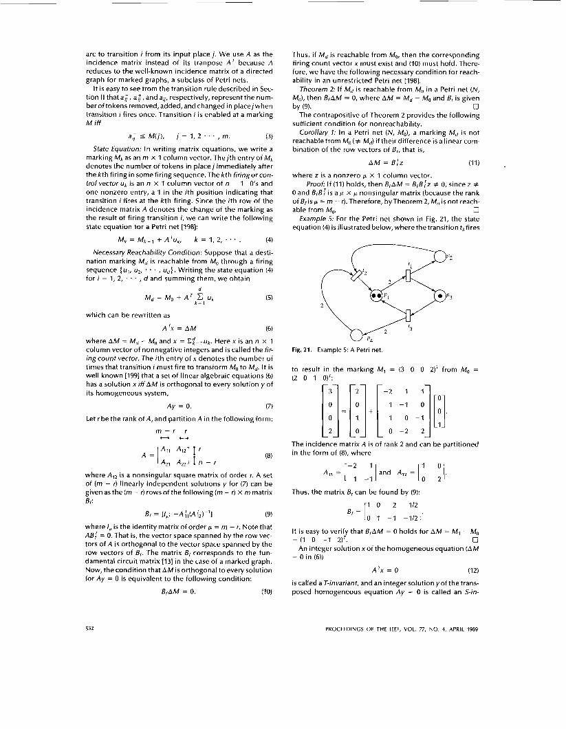
Example 5: For the Petri net shown in Fig. 21, the state equation (4) is illustrated below, where the transition t3 fires

able from MO. 0

Fig. 21. Example 5: A Petri net.

to result in the marking M1 = (3 0 0 2)' from MO = (2 0 1 O ) 5

-1 $1. 2

The incidence matrix A i s of rank 2 and can be partitioned in the form of (8), where

A,, = [ -2 '1 and A,, = [' '1. 1 -1 0 -2

Thw, the matrix Bf can be found by (9):

where I, i s the identity matrix of order p = m - r. Note that AB: = 0. That is, the vector space spanned by the row vectors of A i s orthogonal to the vector space spanned by the row vectors of Bf. The matrix Bf corresponds to the fundamental circuit matrix [I31 in the case of a marked graph.

It is easy to verify that &AM = 0 holds for AM = M1 - MO 0

An integer solution xof the homogeneous equation (AM = (1 0 -1 2IT.

= 0 in (6))

Now, the condition that AM is orthogonal to every solution ATx = 0 (12) for Ay = 0 i s equivalent to the following condition:

i s called a T-invariant, and an integer solution yof the trans- posed homogeneous equation Ay = 0 i s called an S-in- BfAM = 0. (IO)


variant. These invariants which we will discuss in Section Vlll provide powerful tools for studying structural properties of Petri nets.

C. Simple Reduction Rules for Analysis

To facilitate the analysis of a large system, we often reduce the system model to a simpler one, while preserving the system properties to be analyzed. Conversely, techniques to transform an abstracted model into a more refined model in a hierarchical manner can be used for synthesis. There exist many transformation techniques for Petri nets. In this section, we present only the simplest transformations, which can be used for analyzing liveness, safeness, and boundedness. Several transformation rules for marked graphs will be discussed in Section Vll-B2.

It is not difficult to see that the following six operations [179], [203] preserve the properties of liveness, safeness, and boundedness. That is, let (N, MO) and (N’, MA) be the Petri nets before and after one of the following transformations. Then (N’, MA) is live, safe, or bounded i f f (N, MO) i s live, safe, or bounded, respectively.

1) Fusion of Series Places (FSP) as depicted in Fig. 22(a). 2) Fusion of Series Transitions (FST) as depicted in Fig.

3) Fusion of Parallel Places (FPP) as depicted in Fig. 22(c). 4) Fusion of Parallel Transitions (FPT) as depicted in Fig.

5) Elimination ofself-loop Places (ESP) as depicted in Fig.

6) Elimination of Self-loop Transitions (EST) as depicted

22(b).

22(d).

22(e).

in Fig. 22(f).

w

c3 ;I.i x

Fig. 22. Six transformations preserving liveness, safeness, and boundedness.

Example 6:The net shown in Fig. 17(d) can be reduced to theoneshown in Fig.23(a)afterfiringt2to removethetoken in p1 and then fusing tl and f2 into t12, and t3 and t,,into tS4. The net in Fig. 23(a) can then be reduced to the one shown in Fig. 23(b)aftereliminating self-looptransition t12and place p3. It i s easy to see that both nets shown in Fig. 17(d) and Fig. 23(b) are bounded and non-live (and nonreversible).

0

(a) (b) Fig. 23. Example 6: Illustration of reduction rules. The net shown in Fig. 17(d) is reduced to the two nets shown, where all the three nets are bounded, nonlive, and nonreversible.

As pointed out in the introduction, a major weakness of Petri nets i s the complexity problem. Thus, it is very important to develop methods of transformations which allow hierarchical or stepwise reductions and preserve the system properties to be analyzed. Such an approach is discussed in [204], where subnets are reduced to single transitions or places while keeping liveness and/or boundedness properties. However, much work remains to be done in this area of research. For example, given a property or a set of properties, it i s desired to develop a complete set of transformations which allows transformation between any two nets having the given properties. For further information on this subject, the reader i s referred to [200]-[205], [245], [246], and [256].

VI. CHARACTERIZATIONS OF LIVENESS, SAFENESS, AND

REACHABILITY

In this section, we first discuss some subclasses and then liveness, safeness, and reachabilitycriteriawithin each subclass of Petri nets.

A. Subclass of Petri Nets

Recall that a Petri net i s called ordinarywhen all of its arc weights are 1’s. All Petri nets considered in this section are ordinary. Note that both ordinary and nonordinary Petri nets have the same modeling power. The only difference is modeling efficiency or convenience.

We use the following symbols for a pre-set and a post-set (where F is the set of all arcs defined in Table 2):

*t = { pJ(p, t ) E f } = the set of input places of t

t* = {pJ(t, p) E F } = the set of output places of t

*p = {tJ(t, p) E F } = the set of input transitions of p

p* = {tl(p, t) E F } = the set of output transitions of p.

The above symbols are illustrated in Fig. 24. This notation can be extended to a subset. For example, let S1 E P, then *S1 i s the union of all *p such that p E S1. With the above notation, we can now define subclasses of Petri nets by imposing some restrictions on their underlying structures [8], [206], [207l. Unless otherwise stated, it i s assumed throughout this paper that a net N has no isolated places and transitions, i.e., no p or t such that *p = p* = 0 or *t = t. = 0.


Input transitions

of P .P

output placcs o f t

1 .

output

O f P

transitions

P.

(b)

Fig. 24. The symbols for (a) the sets of input and output places of t , and (b) the sets of input and output transitions of p.

1) A state machine (SM) is an ordinary Petri net such that each transition t hasexactlyone input place and exactlyone output place, i.e.,

lot1 = (t.1 = 1 for all t E T.

2) A markedgraph (MG) i s an ordinary Petri net such that each place p has exactly one input transition and exactly one output transition, i.e.,

1 . ~ 1 = Jp.1 = 1 for all p E P.

3) A free-choice net (FC) i s an ordinary Petri net such that every arc from a place i s either a unique outgoing arc or a unique incoming arc to a transition, i.e.,

for all p E P, I p.1 I 1 or = { p}; equivalently,

for all pl, p2 E P, pl* n p2. f 0 = > Ipl*l = lp2*l

= 1.

4) An extended free-choice net (EFC) i s an ordinary Petri net such that

pl* fl p p # 0 = > p1* = p2* for all pl, p2 E P.

5) An asymmetricchoice net (AC) (also known as a simple net) i s an ordinary Petri net such that

1. 2 P2* pl* r l p2* # 0 = > pl* E p2* or p

for all pl, p2 E P.

The Petri net structures shown in Fig. 25 are the key structures that characterize these subclasses. I t i s easy to rec- ognize the key structures of S M s and MGs shown in Fig. 25(a) and (b), respectively. FCs are a generalization of the structures common to both S M s and MGs. They allow the conflict structure of SM shown in Fig. 25(a) and the synchronization structure of MG shown in Fig. 25(b), but exclude the structure shown in Fig. 25(c), where pl* = p2* = {tl , f 2 } . Extended free choice nets (EFC) allow the structure shown in Fig. 25(c) but not the one shown in Fig. 25(d), where p1* = { t , } E p2* = { t , , t 2 } . Both FCs and EFCs have the behavioral property that if tl and t2 share a common input place, then there are no markings for which one i s

( f ) Fig. 25. Key structures characterizingubclasses of Petri nets and their Venn diagram, where MC, m, etc., denote nonMC, nonSM, etc.

enabled and the other i s disabled. Thus, we have “free- choice”aboutwhich transition to fire. In this sense, the EFC structure shown in Fig.25(c)can betransformed to itsequiv- alent FC structure as is illustrated in Fig. 26 [207]. Asym- metric choice nets (AC) allow the structure shown in Fig. 25(d) but not the structureof aconfusion shown in Fig. 25(e), wherepp = {tl, t2 } andp2. = { t2 , t 3 } . Unlikethe behavioral property of FCs and EFCs, ACs can have a marking at which tl i s enabled but t2 i s disabled.

In summary, SMs admit no synchronization, MGs admit no conflicts, FCs admit no confusion, and ACs allow asymmetric confusion (Fig. 7(b) but disallow symmetric confusion (Fig. 7(a)). Their Venn diagram relation i s shown in Fig. 25(f).

Example 7: We apply the above classification of subclasses to classify the nets shown in Fig. 17. The net shown

t ‘2

t ‘2

Fig. 26. Transformation of EFC structure to FC structure.


in Fig. 17(a) is not an AC because p3* = { t l , t 2 } , p4* = { t , , t 4 } , p3* f3 p4* # 0, but one is not a subset of the other. The net in Fig. 17(c) i s FC since each place has a unique outgoing arc. The nets in Fig. 17(d) and (g) are ACs since p3* = { t3} C p2* = { t , , f3} in Fig. 17(d) p3* = { t2} C p2* = { t2, t4 } and ps* = I t 4 } C p2* = { t2 , f4} in Fig. 17(g). The net in Fig. 17(f) i s not an AC because p2* = { tl , t 4 } and p3* = { t , , t5} . The net in Fig. 17(h) i s both an MC and an SM. The net in Fig. 17(e) i s an MG.

B. Liveness and Safeness Criteria

7) Existence of Live-Safe Markings: Live and safe Petri nets (LSPNs) are fundamental to both the applications and theoretical developments of Petri nets. In this section, we present liveness and safeness conditions for subclasses of Petri nets.

First, we discuss necessary conditions for existence of an LS marking MO for a Petri net structure PN. A place p (transition t ) i s said to be a source place (source transition) if *p = 0 ( e t = @).Aplacep(transition t)issaidtobeasinkplace (sink transition) if p* = 0 ( t * = 0). It i s not difficult to see the following theorem [208] from Table 3.

Table 3 Explanation as to Why a Live and Safe Petri Net Cannot Have Source or Sink Places and Transitions

Case If such as then

1 * p = 0 /T: t is not live. (source place) P O+n t .

\ 2 p * = 0 -\ p is not safe for live t.

(sink place) Y-" P

3 * t = 0 t 0-G p p is not safe.

4 t * = 0 .\ t i s not live for safe p.

(source transition) L

(sink transition)

Theorem 3: If a Petri net (N, MO) i s live and safe, then there are no source or sink places and source or sink transitions, i.e., for all x E P U T, *X # 0 # X* 0

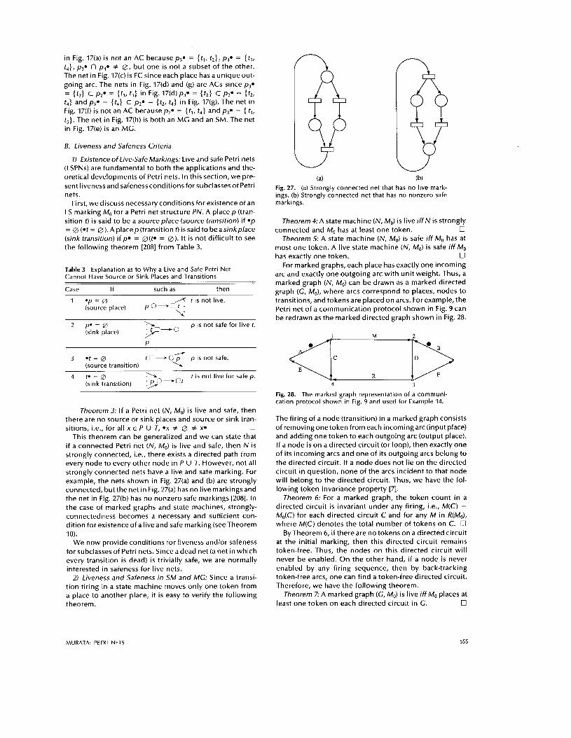
This theorem can be generalized and we can state that if a connected Petri net (N, MO) i s live and safe, then N i s strongly connected, i.e., there exists a directed path from every node to every other node in P U T. However, not all strongly connected nets have a live and safe marking. For example, the nets shown in Fig. 27(a) and (b) are strongly connected, but the net in Fig. 27(a) has no live markings and the net in Fig. 27(b) has no nonzero safe markings [208]. In the case of marked graphs and state machines, strongly- connectedness becomes a necessary and sufficient condition for existence of a live and safe marking (see Theorem I O ) .

We now provide conditions for liveness andlor safeness for subclasses of Petri nets. Since adead net (a net in which every transition i s dead) is trivially safe, we are normally interested in safeness for live nets.

2) Liveness and Safeness in SM and MG: Since a transition firing in a state machine moves only one token from a place to another place, it i s easy to verify the following theorem.

4p I Y W

(a) (b) Fig. 27. (a) Strongly connected net that has no live markings. (b) Strongly connected net that has no nonzero safe markings.

Theorem 4: A state machine (N, MO) i s live i f f N i s strongly 0

Theorem 5: A state machine (N, MO) i s safe iff Ma has at most one token. A live state machine (N, MO) i s safe iff MO

For marked graphs, each place has exactly one incoming arc and exactly one outgoing arc with unit weight. Thus, a marked graph (N, MO) can be drawn as a marked directed graph (G, MO), where arcs correspond to places, nodes to transitions, and tokens are placed on arcs. For example, the Petri net of a communication protocol shown in Fig. 9 can be redrawn as the marked directed graph shown in Fig. 28.

connected and MO has at least one token.

has exactly one token. 0

Fig. 28. The marked graph representation of a communication protocol shown in Fig. 9 and used for Example 14.

The firing of a node (transition) in a marked graph consists of removing one token from each incoming arc (input place) and adding one token to each outgoing arc (output place). If a node is on a directed circuit (or loop), then exactly one of i t s incoming arcs and one of its outgoing arcs belong to the directed circuit. If a node does not lie on the directed circuit in question, none of the arcs incident to that node will belong to the directed circuit. Thus, we have the following token invariance property [q.

Theorem 6: For a marked graph, the token count in a directed circuit i s invariant under any firing, i.e., M(C) = Mo(C) for each directed circuit C and for any M in /?(Ma), where M(C) denotes the total number of tokens on C. 0

By Theorem 6, if there are no tokens on a directed circuit at the initial marking, then this directed circuit remains token-free. Thus, the nodes on this directed circuit will never be enabled. On the other hand, if a node is never enabled by any firing sequence, then by back-tracking token-free arcs, one can find a token-free directed circuit. Therefore, we have the following theorem.

Theorem 7: A marked graph (G, MO) is live iff MO places at least one token on each directed circuit in G. U


The following theorem is a special case of more general theoremswhich will be proved in Section VI1 (weighted sum of tokens) and Section VI11 (S-invariants).

Theorem 8: The maximum number of tokens that an arc can have in a marked graph (G, MO) is equal to the minimum number of tokens placed by MO on a directed circuit con-

The following consideration i s helpful in understanding the above mini-max theorem. Consider all directed circuits C,, C,, . . . , C, passing through the arc e. Bring as many tokens as possible on the incoming arcs of the initial node x of e = (x, y), and fire the nodex as many times as possible without firing the node y. It can be seen that Min {Mo(C1), Mo(C2), . . . , Mo(Cm)} is the maximum possible tokens that can be brought on the arc e. In particular, if Min {M&C!), Mo(C2), . . . , Mo(C,)} = 1, then M(e) 5 1 for all M in /?(MO). Thus, we have the following theorem.

Theorem 9: A live marked graph (G, MO) i s safe i f f every arc (place) belongs to a directed circuit C with Mo(C) = 1.

Theorem 70: There exists a live and safe marking in a directed graph G iff C i s stongly connected.

Proof: The necessity i s due to Theorem 3. The sufficiency can be proved as follows. Suppose G is strongly connected. Choose a marking MO which places at least one token in each directed circuit in G. Then this marked directed graph, (G, MO) is live. If (G, MO) i s not safe, then there i s an arc e and a marking M in /?(MO) such that M(e) 2 2. Reduce the number of tokens on e to one by removing tokensfrome;callthenewmarkingM’, i.e.,M‘(e) = 1. Repeat the above token removal which will not destroythe liveness property, until (G, M,”) i s safe for a new marking M;. U

A subset of arcs E‘ in a directed graph G = (V, E ) i s said to be a feedback arc set (FAS) if G’ = (V, E - E’) i s acyclic, i.e., has no directed circuits. A FAS is said to be minimal if no proper subset of the FAS is a FAS, and minimum if no other FAS contains a smaller number of arcs. It is easy to see that the subset of marked arcs in a live marked graph is a FAS. Conversely, if each arc in a FAS of a directed graph is marked, we have a live marked graph. Furthermore, the following theorem [209] holds.

Theorem 11: A strongly-connected live marked graph G i s safe iff for every marking M in /?(MO), the set of marked arcs i s a minimal FAS.

A minimum FAS is more important than a minimal FAS in applications. It is obvious that a subset E’ in a directed graph G is a minimum FAS iff the marking M such that M(e) = 1 for all e in E’ is a live marking for G with the minimum number of tokens. However, a minimum FAS does not necessarily yield a safe marking. For example, the marking MO shown in Fig. 29 is a live markingwith the minimum number of tokens and corresponds to a minimum FAS (G becomes acyclic if the two marked arcs a and b are removed), How- ever,thismarking isnotsafesincearcsdand fdonotbelong

taining this arc. 0

Fig. 29. The set of marked arcs a and b i s a minimum feedback arc set, and this marking i s minimally live but not safe.

to a directed circuit with token count one. In fact, the firing sequence U = (1 3 4 1) brings two tokens on arc d.

3) Liveness and Safeness in FC and AC Nets: Siphon and trap: A nonempty subset of places S in an

ordinary net N i s called a siphon (also known as a deadlock) if *S s So, i.e., every transition having an output place in Shasan inputplaceinS.(Weuseasiphon insteadofadead- lock since the latter i s used for a circular waiting condition or behavior in computer science). A nonempty subset of places Q in an ordinary net N is called a trap if Qa E *Q, i.e., every transition having an input place in Q has an output place in Q. A siphon is illustrated in Fig. 30(a), where

P

a s = { [ , } Q‘ = I l l }

S . = { I I } *Q=It,,t,} 1’ 2

. S E S . Q- c -Q (a) (b)

Fig. 30. Illustration of (a) a siphon and (b) a trap.

the token count in the siphon remains the same by firing t , but decreases by firing t2. Thus, a siphon has a behavioral property that if it is token-free under some marking, then it remains token-free under each successor marking. A trap is illustrated in Fig. 30(b), where the token count in the trap remains the same by firing t, but increases by firing f 2 . Thus, a trap has a behavioral property that if it i s marked (i.e., it has at least one token) under some marking, then it remains marked under each successor marking. It i s easy to verify that the union of two siphons (traps) i s again a siphon (trap). A siphon (trap) is called a basic siphon (basic trap) if it cannot be represented as a union of other siphons (traps). All siphons (traps) in a Petri net can be generated by the union of some basis siphons (traps) [210]. A siphon (trap) i s said to be minimal i f it does not contain any other siphon (trap). A minimal siphons (traps) are basis siphons (traps), but not all basis siphons (traps) are minimal.

Example8: In the Petri net shown in Fig. 31, let SI = { p,,

and S5 = { p2, p3, p4} . Then, we have *S1 = { tl , f 2 , t4} E S,* = {t,, f 2 , f 3 , t4} . Thus, SI is a siphon. Since S4. = {t,, t4} E *S4 = { t , , f 2 , f4}, S4 i s a trap. Similarly, it i s easy to verify that S2 is a siphon, S3 i s both a siphon and a trap, and S5 i s a trap. In fact, both S1 and S2 are minimal and basis siphons. S3, S4, and S5 are basis traps, S3 and S5 are not minimal traps.

Siphons and traps can be found from a set of logic equations or linear inequalities describing their behavioral properties [179]. For example, in the Petri net shown in Fig.

p2, p3) I s2 = { PI, p2, p4} I s3 = { p1, p2, p3r p4) I s4 = { p2, p31


I

Fig. 31. The net used in Examples 8 and 9.

31, we see that

P1 => p2

p2 => p3 V p4

p3 => p1 A p2

P4 => P1

(if p1 i s in a siphon S, then p2 i s in S )

(if p2 is in S, then p3 or p4 i s in S )

(if p3 is in S, then p1 and p2 are in S)

(if p4 i s in S, then p1 i s in S).

The above set of “if-then” rules is equivalent to the following set of clauses:

{ T P l v P2r 7 P 2 v p3 v p4, -7p3 v p1,

7 P 3 v P2r 7p4 v P l ) .

Thus, siphons can be found as (0,l)-solutions of the following set of inequalities, where p, = 1 if p, E S, and p, = 0 if p, $ S:

-p1 + p2 5 0

-pz + p3 + p4 1 0

-p3 + p1 1 0.

-P3 + p2 2 0

-p4 + p1 1 0

U For example, pl = p2 = p3 = 1, p4 = 0 satisfy the above inequalities. Therefore, { pl , p2, p3 } is a siphon.

The following theorems are well known in the literature [207l, [211]. However, since their proofs are beyond the scope of this paper, they are omitted. Examples are given to illustrate the theorems.

Theorem 12: A free-choice net (N, MO) i s live iff every

Theorem 13: A live free-choice net (N, MO) i s safe iff N i s covered by strongly-connected SM components each of

0 Theorem 74: Let (N, MO) be a live and safe free-choice net.

Then, N i s covered by strongly-connected MG components. Moreover, there i s a marking MeR(M0) such that each component (NI, M1) is a live and safe MG, where M1 i s M restricted to N1. 0

Theorem 75: An asymmetric choice net (N, MO) i s live if (but not only i f) every siphon in N contains a marked trap.

0 In Theorem 13 (Theorem 14), an SM-component (MG-

component) N1 of a net N is defined as a subnet generated by places (transitions) in NI having the following two properties: i) each transition (place) in NI has at most one incom-

r siphon in N contains a marked trap.

which has exactly one token at MO.

n

ing arc and at most one outgoing arc; and ii) a subnet generated by places (transitions) i s the net consisting of these places (transitions), all of their input and output transitions (places), and their connecting arcs. Theorem 13 (Theorem 14) leads to the observation [211] that a live and safe free- choice net can be viewed as an interconnection of live and safe state machines (marked graphs). This observation i s useful for many applications including decompositions and abstraction of Petri nets [205].

Example 9: The FC net shown in Fig. 31 i s not live since the siphon { pl , p2, p4 } contains no traps (thus no marked traps). The AC net shown in Fig. 32 i s live since the minimal

Fig. 32. A

3

I

live AC net.

siphon { pl, p3, p4} contains a marked trap { pl , p3, p4} and the siphon { pl, p2, p3, p4) contains marked traps { pl , p2} and { pl , p3, p4 } . The live FC net shown in Fig. 33(a) i s not safe and the safe FC net shown in Fig. 33(b) i s not live since

h

(b) Fig. 33. (a) A live, nonsafe FC net. (b) A safe, nonlive FC net.

these nets are not covered by strongly connected MG components (nor by strongly connected SM components). The net shown in Fig. 34 i s live and safe but is not covered by strongly-connected MG components since it i s not FC. The AC net shown in Fig. 34 i s live since every siphon contains a marked trap. However, the AC net shown in Fig. 35 i s live even though the siphon { p1,p2,p3,p4} contains no marked traps (see Theorem 15). The live and safe FC net shown in Fig. 36(a) i s covered by the two strongly-connected MG components shown in Fig. 36(b). It i s also covered by the two strongly-connected SM components shown in Fig. 36(c). 0


U

‘3

Fig. 34. A live and safe AC net.

p4

Fig. 35. A live AC net.

It i s known that an asymmetric choice net (N, MO) i s live if7 it is place-live, i.e., for each M, in R(Mo) and for each place p in N, there exists a marking M in R(Ml) such that M(p) > 0. The Petri net shown in Fig. 17(a) i s place-live, but it i s not live since tl is dead. Another useful property of asymmetric choice nets is that the conflict relation i s transitive. For example, in the asymmetric choice net shown in Fig. 37(a), any pair of transitions among tl, t2, and t3 are in a conflict relation. However, in the net shown in Fig. 37(b), which i s not an asymmetric choice net, the pair (tl, t2) is in conflict and the pair (t2, r3) i s in conflict but (tl, t3) i s not in conflict.

References [ I l l , [206]-[208], [211], and [2141 are suggested for further reading on free-choice nets and other topics discussed in this section.

C. Reachability Criteria

a nonnegative integer solution x satisfying (6) or In Section V-B, it has been shown that the existence of

Md = MO -t A J x (1 3)

i s a necessary condition for Md to be reachable from MO. A Petri net having no directed circuits i s called an acyclic Petri net. For this subclass, it can be shown [212] that this condition is necessaryand sufficient. Given a nonnegative integer solution x satisfying (13), let N, denote the (firing count) subnet of N consisting of transitions t such that x( t ) > 0, together with their input and output places and their connecting arcs. MO, denotes the subvector of MO for places in N X .

Theorem 76: In an acyclic Petri net, Md i s reachable from M,iffthereexistsa nonnegative integer solutionx satisfying (13).

Proof: Only sufficiency remains to be shown. Suppose there exists such a solution x. Consider the subnet (N,, MO,),

U

‘2

f \

(C) Fig. 36. (a) A live and safe FC net. (b) Its two strongly-connected MG-components generated by the two sets of transitions {tl, t3, t,, r,} and { t2, rs, r6, t , } , respectively. (c) Its two strongly-connected SM-components generated by the two setsof places {p1,pz,p4,p61 and {p1,p3,p5,p7J, respectively.

which is acyclic. There i s at least one transition t that i s firable at MO,. (If not, back-tracing token-free input places of nonfirable transitions would end at a token-free source place p. This contradicts the fact that Md 2 0.) Now, fire t.


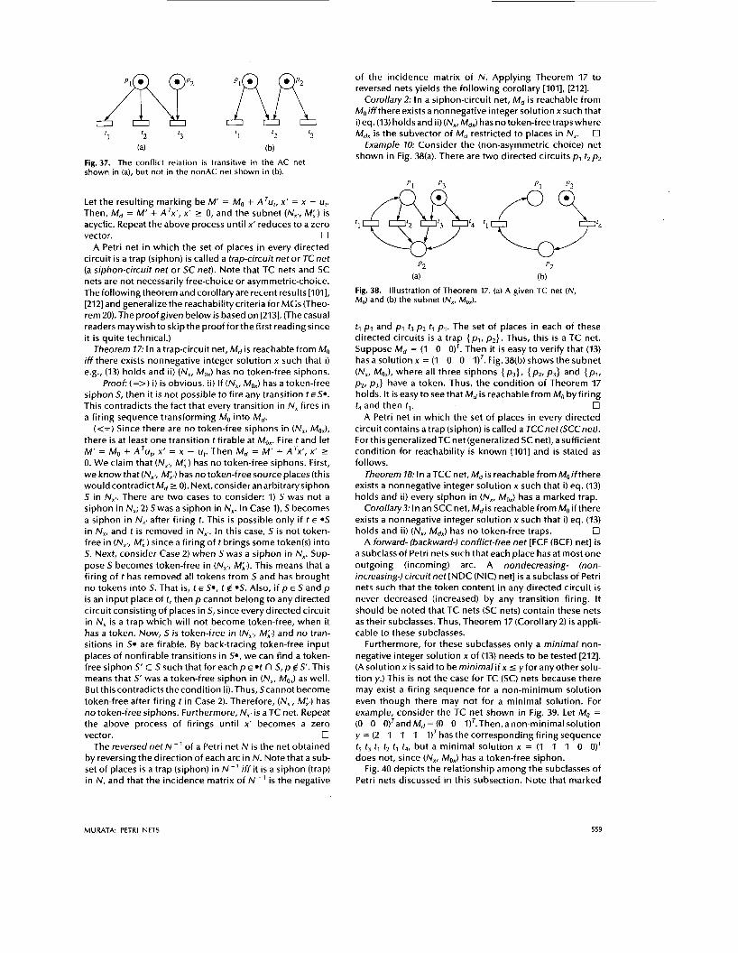
of the incidence matrix of N. Applying Theorem 17 to reversed nets yields the following corollary [ lol l , [212].

Corollary2: In a siphon-circuit net, Md i s reachable from Moiff there exists a nonnegative integer solution x such that i) eq. (13) holds and ii) (N,, Mdx) has no token-free traps where

(a) (b) Example 70: Consider the (non-asymmetric choice) net shown in Fig. 38(a). There are two directed circuitspl t 2pz

t r '2 '3 Mdx i s the subvector of Md restricted to places in N,. 0 ' 2 [3

Fig. 37. The conflict relation is transitive in the AC net shown in (a), but not in the nonAC net shown in (b).

Then, Let the Md resulting = M' + marking A'x', x' be L 0, M' and = MO the + subnet A'u,, x' (N,,, = x Mi.) - ut. i s at4 ', 0 acyclic. Repeat the above process until x' reduces to a zero f

vector. 17 A Petri net in which the set of places in every directed

circuit i s a trap (siphon) i s called a trap-circuit net or TCnet (a siphon-circuit net or SC net). Note that TC nets and SC nets are not necessarilv free-choice or asvmmetric-choice.

'1

p2 p2

(a) (b)

The following theorem and corollaryare recent results [IOI], [212] and generalize the reachability criteria for MGs (Theo- rem 20). The proof given below is based on [213]. (The casual readersmaywish toskipthe proofforthe first reading since it i s quite technical.)

Theorem 77: In a trap-circuit net, Md is reachable from MO iff there exists nonnegative integer solution x such that i) e.g., (13) holds and ii) (N,, MO,) has no token-free siphons.

Proof: (=>) i) is obvious. ii) If (N,, MO,) has a token-free siphon S, then it i s not possible to fire any transition t €9. This contradicts the fact that every transition in N, fires in a firing sequence transforming MO into Md.

(<=) Since there are no token-free siphons in (N,, MO,), there i s at least one transition t firable at MO,. Fire t and let M' = MO + A'u,, X' = x - ut. Then Md = M' + A'x', X' L 0. We claim that (N,,, M;.) has no token-free siphons. First, we know that (N,,, Mi,) has no token-free source places (this would contradict Md L 0). Next,consideran arbitrarysiphon S in N,.. There are two cases to consider: 1) S was not a siphon in N,; 2) S was a siphon in N,. In Case I), S becomes a siphon in N,. after firing t . This i s possible only if t E *S in N,, and t i s removed in N,,. In this case, S i s not token- free in (Nx,, Mi,) since a firing o f t brings some token(s) into S. Next, consider Case 2) when S was a siphon in N,. Sup- pose S becomes token-free in (N,,, Mi,). This means that a firing of t has removed all tokens from S and has brought no tokens into S. That is, t E So, t $ *S. Also, if p E S and p i s an input place of t , then p cannot belong to any directed circuit consisting of places in S, since every directed circuit in N, i s a trap which will not become token-free, when it has a token. Now, S i s token-free in (N,., M;.) and no transitions in S* are firable. By back-tracing token-free input places of nonfirable transitions in So, we can find a token- free siphon s' c S such that for each p E *t n S, p $ s'. This means that S' was a token-free siphon in (Nx, MO,) as well. Butthiscontradicts thecondition ii).Thus,Scannot become token-free after firing t in Case 2). Therefore, (N,,, Mi,) has no token-free siphons. Furthermore, N,. is a TC net. Repeat the above process of firings until x' becomes a zero vector . 17

The reversednet N -' of a Petri net N is the net obtained by reversing the direction of each arc in N. Note that a subset of places is a trap (siphon) in N -' iff it i s a siphon (trap) in N, and that the incidence matrix of N -' is the negative

Fig. 38. Illustration of Theorem 17. (a) A given TC net (N, MO) and (b) the subnet ( N x , Max).

tl p1 and p1 t3 p2 tl pl. The set of places in each of these directed circuits i s a trap { pl, p2} . Thus, this is a TC net. Suppose Md = (1 0 0)'. Then it i s easy to verify that (13) has a solution x = (1 0 0 I)'. Fig. 38(b) shows the subnet (Nx, MO,), where all three siphons { p3} , { p2, p3} and { pl, p 2 , p3} have a token. Thus, the condition of Theorem 17 holds. It i s easy to see that Md i s reachable from MO by firing t4 and then t , . 17

A Petri net in which the set of places in every directed circuit contains a trap (siphon) i s called a TCCnet(SCCnet). For this generalized TC net (generalized SC net), a sufficient condition for reachability is known [ IO11 and is stated as follows.

Theorem 78: In a TCC net, Md is reachable from Moifthere exists a nonnegative integer solution x such that i) eq. (13) holds and ii) every siphon in (N,, MO,) has a marked trap.

Corollary3: In an SCC net, Md i s reachable from MO if there exists a nonnegative integer solution x such that i) eq. (13)

0 A forward- (backward-) conflict-free net [FCF (BCF) net] i s

a subclass of Petri nets such that each place has at most one outgoing (incoming) arc. A nondecreasing- (non- increasing-) circuit net [NDC (NIC) net] is a subclass of Petri nets such that the token content in any directed circuit i s never decreased (increased) by any transition firing. It should be noted that TC nets (SC nets) contain these nets as their subclasses. Thus, Theorem 17 (Corollary 2) i s applicable to these subclasses.

Furthermore, for these subclasses only a minimal nonnegative integer solution x of (13) needs to be tested [212]. (A solution x is said to be minimal if x 5 yfor any other solution y.) This is not the case for TC (SC) nets because there may exist a firing sequence for a non-minimum solution even though there may not for a minimal solution. For example, consider the TC net shown in Fig. 39. Let MO = (0 0 0)'and Md = (0 0 l)T.Then,anon-minimalsolution y = (2 1 1 1 1)'has the corresponding firing sequence ts t3 tl t2 tl t4, but a minimal solution x = (1 1 1 0 0)' does not, since (Nx, MO,) has a token-free siphon.

Fig. 40 depicts the relationship among the subclasses of Petri nets discussed in this subsection. Note that marked

holds and ii) (N,, Mdx) has no token-free traps.


or

Fig. 39. A TC net which is not a FCF net.

Ordinary Petri Nets

Fig. 40. Relationship among subclasses of Petri nets for which reachability criteria are known.

graphs are contained in the intersection of all these subclasses.

VII. ANALYSIS AND SYNTHESIS OF MARKED GRAPHS

Among models that can represent concurrent activities, marked graphs are the most amenable to analysis. Marked graphs basically model decision-free (or deterministic) concurrent systems. A marked graph representation of a system with decisions i s possible only if each decision can be embedded in a single-entry-and-single-exit subsystem because this subsystem can then be represented by a place having exactly one incoming and one outgoing arc. This section presents detailed discussions on analysis and synthesis techniques for marked graphs.

A. Reachability in MGs

As stated in Section V-B, the incidence matrix A of a marked graph (G, MO) corresponds to the node-to-arc incidence matrix of its underlying directed graph or digraph G. The matrix Bf of a marked graph (G, MO), which i s defined by (9), corresponds to the fundamental circuit matrix Bf of G [131. It i s well known that the two matrices are orthogonal to each other, i.e.,

BfA' = 0. (1 4)

If a marking Md is reachable from MO through a firing sequence U in a marked graph (G, MO), we can write (6) or

A'x = AM (1 5)

where AM = Md - MO and x = 3 = the firing count vector of the firing sequence U. From (14) and (15), we have

Equation (17) states that the algebraic sum of tokens placed by MO on a fundamental circuit i s equal to that placed by Md. Equation (17) is ageneralization of the token invariance on a directed circuit (Theorem 6). Equation (16) has an interpretation like Kirchhoff'svoltage law (KVL) in circuittheory. It has been shown [215] that this generalized token invariance expressed by (17) i s not only necessary but also sufficient for a live marking MO to reach another marking M+ In other words, we have the following theorem.

Theorem 79: In a live marked graph (C, MO), Md i s reach- 0

Note that if G i s strongly connected, then condition (17) is equivalent to saying that the token count on each directed circuit under MO i s the same as that under Md, i.e., Mo(C) = Md(C) for each directed circuit C in G.

The above theorem can be extended to nonlive marked graphs if one imposes the additional condition that the nodes (transitions) that are to fire should not lie on a token- free directed circuit. In other words, we have the following theorem [215].

Theorem 20: In a marked graph (G, MO), Md i s reachable from Moiff (17) holds and for the minimal nonnegative solution x for A'x = AM, no nodes t such that x(t) > 0 are on

0 The above theorem has been further generalized to sub-

marking reachability [216], [217]. Since every marked graph is a TC net as well as an SC net, both Theorem 17 and Cor- ollary 2 reduce to Theorem 20.

Example 77: Consider the marked graph (C, MO) shown in Fig. 41, where C i s not strongly connected and MO is not a

able from MO iff (17) holds.

any token-free directed circuit in (G, MO).

M O Md

Fig.41. The marked graph for Example 11 to illustrate reachability conditions.

safe marking. The fundamental circuit matrix Bfwith respect to a spanning tree {d, e, f } for C is given by

a b c d e f

For the two markings MO = (0 0 0 2 1 1)'and M d = (0 0 1 0 0 O)', i t i s easy to verify that (17) holds. Now, (15) for this marked graph can be written as


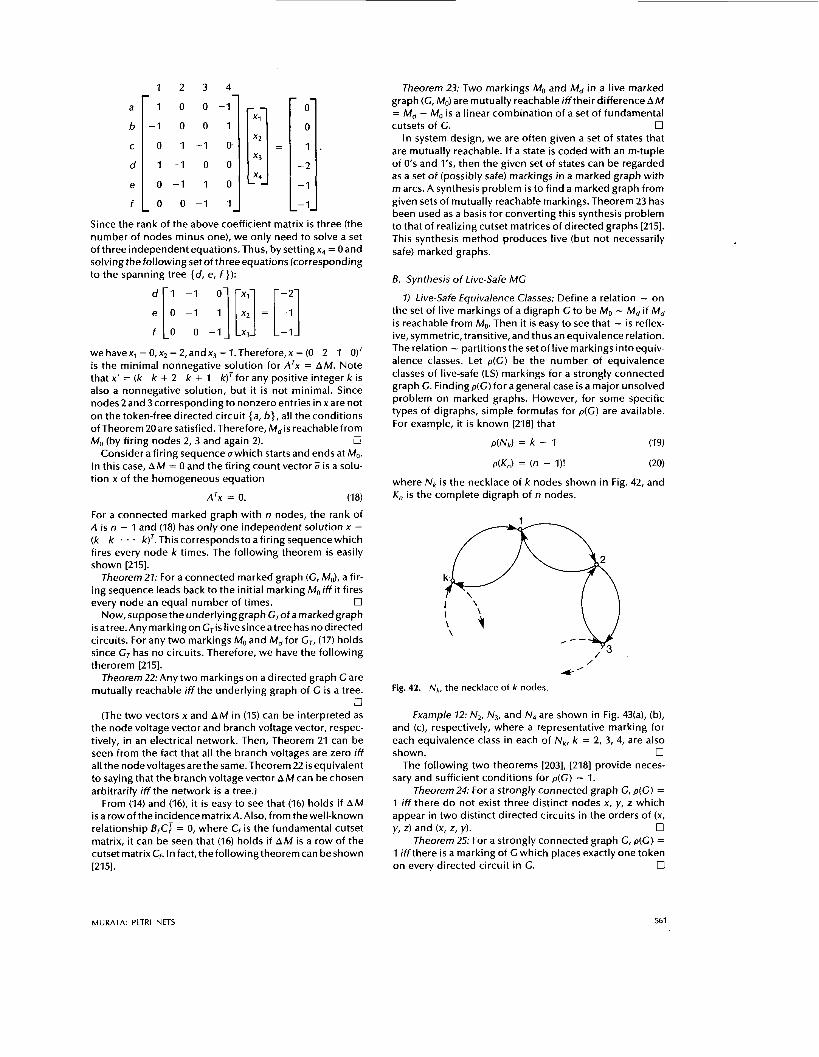
1 2 3 4

1 0 0 - 1

- 1 0 0 1

0 1 - 1 0

1 - 1 0 0

0 - 1 1 0

0 0 - 1 1

0

0

1

-2

-1

-1

Since the rank of the above coefficient matrix is three (the number of nodes minus one), we only need to solve a set of three independent equations. Thus, by settingx, = 0 and solving the following set of three equations (corresponding to the spanning tree {d, e, f }):

wehavexl =0,x~=2,andx3=1.Therefore,x=(0 2 1 0)' i s the minimal nonnegative solution for A'x = AM. Note that x' = (k k + 2 k + 1 k)' for any positive integer k is also a nonnegative solution, but it i s not minimal. Since nodes 2 and 3 corresponding to nonzero entries in x are not on the token-free directed circuit {a, b}, all the conditions of Theorem 20 are satisfied. Therefore, Md is reachable from

0 Consider a firing sequence uwhich starts and ends at MO.

In this case, A M = 0 and the firing count vector ij i s a solution x of the homogeneous equation

A'x = 0. (1 8)

For a connected marked graph with n nodes, the rank of A is n - 1 and (18) has only one independent solution x = (k k . k)'. This corresponds to afiring sequencewhich fires every node k times. The following theorem i s easily shown [215].

Theorem 21: For a connected marked graph (G, MO), a firing sequence leads back to the initial marking &i f f it fires

0 Now, suppose the underlying graph G,of a marked graph

i s atree. Any marking on G'is livesinceatree has no directed circuits. For any two markings MO and Md for GT, (17) holds since GT has no circuits. Therefore, we have the following therorem [2151.

Theorem 22:Any two markings on a directed graph G are mutually reachable i f f the underlying graph of G i s a tree.

0 (The two vectors x and A M in (15) can be interpreted as

the node voltage vector and branch voltage vector, respectively, in an electrical network. Then, Theorem 21 can be seen from the fact that all the branch voltages are zero i f f all the nodevoltages arethe same.Theorem 22 isequivalent to saying that the branch voltage vector A M can be chosen arbitrarily i f f the network i s a tree.)

From (14) and (16), it i s easy to see that (16) holds if A M is a row of the incidence matrix A. Also,from the well-known relationship BfC: = 0, where Cf i s the fundamental cutset matrix, it can be seen that (16) holds if A M i s a row of the cutset matrix Cf. In fact, the following theorem can be shown [215].

MO (by firing nodes 2, 3 and again 2).

every node an equal number of times.

Theorem 23: Two markings MO and Md in a live marked graph (GI MO) are mutually reachable iff their difference A M = Md - MO i s a linear combination of a set of fundamental cutsets of G. 0

In system design, we are often given a set of states that are mutually reachable. If a state i s coded with an m-tuple of 0's and Ifs, then the given set of states can be regarded as a set of (possibly safe) markings in a marked graph with m arcs. A synthesis problem i s to find a marked graph from given sets of mutually reachable markings. Theorem 23 has been used as a basis for converting this synthesis problem to that of realizing cutset matrices of directed graphs [215]. This synthesis method produces live (but not necessarily safe) marked graphs.

B. Synthesis o f Live-Safe MG

1) Live-Safe Equivalence Classes: Define a relation - on the set of live markings of a digraph G to be MO - Md if Md i s reachable from MO. Then it is easy to see that - i s reflex- ive, symmetric, transitive, and thus an equivalence relation. The relation - partitions the set of live markings intoequiv- alence classes. Let p ( G ) be the number of equivalence classes of live-safe (LS) markings for a strongly connected graph G. Findingp(G) for a general case i s a major unsolved problem on marked graphs. However, for some specific types of digraphs, simple formulas for p(G) are available. For example, it i s known [218] that

(19)

(20)

where Nk is the necklace of k nodes shown in Fig. 42, and K,, i s the complete digraph of n nodes.

p(Nk) = k - I

p(KJ = (n - I)!

/

4' Fig. 42. Nk, the necklace of k nodes.

Example 12: NZ, N3, and N4 are shown in Fig. 43(a), (b), and (c), respectively, where a representative marking for each equivalence class in each of Nk, k = 2, 3, 4, are also shown. 0

The following two theorems [203], [218] provide necessary and sufficient conditions for p ( G ) = 1.

Theorem 24: For a strongly connected graph G, p ( G ) = 1 iff there do not exist three distinct nodes x, y, z which appear in two distinct directed circuits in the orders of (x,

0 Theorem 25: For a strongly connected graph G, p(G) =

1 iff there i s a marking of G which places exactly one token 0

y, z) and (x, z, y).

on every directed circuit in G.


L

N2

(a) 00 0

3 N 3

3

(b)

d

C c

N4

(d Fig. 43. (a) An example of p ( G ) = 1, G = N,. (b) An example of p ( G ) = 2, G = N, (c ) An example of p ( G ) = 3, G = N+

Example 73: In the marked graphs shown in Fig. 43(c), p(N4) # 1 since there are three distinct nodes 1, 2, 3 such that the sequence (1 2 3) i s in the outer directed circuit, {a, b, c, d } , and the sequence (1 3 2) is in the inner directed circuit {e, f, g, h } (Theorem 24). Also, it can be seen that there is no marking M such that M(C) = 1 for every directed circuit in N4. In the marked graph (G, MO) shown in Fig. 44, it can be verified that p ( G ) = 1 since MO places

h

3

1 e

4

G3

Fig. 44. A marked graph (G, MO) with p ( G ) = 1.

exactlyone token on each of the following possibledirected circuits in G: {a, b, c}, {b, d, e, f } , { f, g, e}, {a, g, i } , {a, b,d, i } , {b, d,i, h, f } , {c, h, f,b}, and {h, f,g,i} (Theorem 25). 0

= KS.

2) Expansion Rules for LSMG Synthesis: It has been shown [202], [203] that p(G) i s invariant under

the following operations on a digraph C.

a) Series Expansion (SE)-addition of an arc e and node x in series with an existing arc e' (see Fig. 45(a)).

b) ParallelExpansion (PE)-addition of an arc e in parallel with an existing arc e' (see Fig. 45(b)).

c) Unique-Circuit Expansion WE)-addition of an arc e = (vl , v2) to a unique directed path P21 from v2 to v1 (see Fig. 45(c)).

d) V-Y Expansion (VYE)-addition of a node x and an arc e = (x, y) to a pair of existing arcs el = ( y, z) and e2 = ( y, w) (also applicable if (CY, /3) is replaced by (/3, C Y )

everywhere) (see Fig. 45(d)). e) Separable Graph Expansion (SCE)-joining two

graphs G1 and G2 at exactly one node x to produce a separable graph G (see Fig. 45(e)). In this expansion, we have p(G) = p(G1) p(G2). Thus, p(G) = 1 is invariant iff p(G1) = P(G2) = 1.

Theabovestepwiseexpansion operationscan be used for synthesizing LSMCs (G, MO). In this synthesis, the following properties of decision-free concurrent systems can be prescribed: liveness (absence of deadlocks), safeness (absence of overflows), p(G) = 1 (all LS markings or states are mutually reachable), minimum cycle time, and resource require- ments [219]. Note that, in order to maintain the liveness and safeness properties, the newly added arc e must be token- free in the series and V-Y expansions, M(e) = M(e') in the


0 - E3 1 e’ 2

0 - m 1 e’ 2

p21 ,.---. \

8’ b e 1 2

or

Fig. 45. Illustration of the five expansion rules (a) series expansion, (b) parallel expansion, (c) unique circuit expansion, (d) V-Y expansion, and (e) separate graph expansion

parallel expansion, and M(e) = 1 after making the unique path P21 token-free by appropriate firings.

Example 74: The LSMG model (Cl, MO) of a communication protocol shown in Fig. 28 can be synthesized from N 2 by applying the above expansion rules six times. This is illustrated in Fig. 46, where PE(.), SE(-), and UE(-) denote

L

0 UE (B) a:-pq:D; SE (F)

R R

G1

Fig. 46. Illustration of the use of expansion rules for LSMG synthesis.

parallel, series, and unique circuit expansions, respectively, and the labels inside the parentheses indicate the arcs added by the expansions. Thus, we have p(Cl) = p(N2) = 1. By applying the SGE rule to n necklaces of 2 nodes (N2) ,

0

0 0

G2

Fig. 47. A LS marked graph model of an n-stage pipeline operation.

we know that p(G2) = 1 for the marked graph (G2, MO) of an n-stage pipeline operation shown in Fig. 47. The reverse operations of the above expansions are the reduction rules that can be used to find p(G) for a given digraph G. For example, it is easy to verify that the marked graph (G3, MO) shown in Fig. 44 can be reduced to N2 after applying a V-Y reduction first, and then series, parallel, and unique-circuit

0 reductions. Thus, p(G3) = p(N2) = 1.

C. Weighted Sum of Tokens

vector (S-invariant) satisfying Given a marked graph (G, MO), let / be an m x 1 column

A/ = 0 (21 )

whereA i s then x m incidence matrix of G. For any marking M reachable from MO, we have from (15) and (21)

(AM)’/ = (x’A)/ = x’(A/) = 0 (22)

or

MTI = M i / . (23)

Equation (23) states that the weighted sum of tokens ET=, M(ej)/(ei) i s invariant for all markings M reachable from MO. In electrical network terminology, / corresponds to the branch current vector, (21) to Kirchhoff‘s current law, and (22) to Tellegen’s theorem [921.

Let W be an m x 1 column vector whose i th entry is W(e;), a nonnegative integer weight of arc ei. W(e;) may represent the storage space or cost to accommodate a token on arc e;. Then, M’W denotes the weighted sum of tokens for a marking M. Given a bounded live marked graph (G, MO), we are often interested in finding the maximum or minimum valueof MTWforall markings reachable from Mo.Thisvalue can be found from MO and a certain S-invariant / by the following theorem [92].

Theorem 26: For a strongly connected live marked graph (G, MO), we have

max {M‘WIM E /?(MO)} = min {ML/(/ 2 W, A/ = 0)

(24)

min {M’WIM E /?(MO)} = max { M i / [ / 5 W, A/ = 0).

(25)

Proof- Since MO i s live, M E /?(MO) if f M = MO + ATx, where x i s an n x 1 vector of nonnegative integers. Thus, the left-hand side of (24) can be written as the following linear programming problem:

max U = CTz subject to Dz = MO and z 2 0 (26)


where D. Token Distance and Maximum Concurrency

I ) Token Distance Matrix for MG: The token distance t, between two nodes i and j in a marked graph (G, MO) is defined as the minimum token content among all possible directed paths PI, from node i to node j in G, i.e.,

and I,,, is the identity matrix of order m. The dual problem of (26) can be stated as

min V = M l y subject to Dry 2 C (27)

where y = I i s unrestricted. Dry 2 C i s equivalent to I 2 Wand A/ 5 0. However, A/ 5 0 i s equivalent to A/ = 0 since thesumofthenrowsinAisalwayszero,i.e.,[l 1 . . . 1]Al = 0 / = O.Thus,(24)isequivalenttotheproblemon theright- hand side of (27). It i s well known in linear programming that the optimal solution of (26) or (27) i s an extreme point of the corresponding constraint set. Note that all the extreme points of the constraint set have only integral coor- dinates since D is totally unimodular, i.e., every square sub- matrix of D has determinant 0,1, or -1. Therefore, the optimal values of (26) and (27) are attained at integral values, and (24) follows from the theory of duality. Equation (25) can be

Example 15: Consider the marked graph shown in Fig. proved similarly. 0

48, where MO = (1 0 1 0 0)'and W = (1 2 1 2

C O 1

(a)

"- C O I

(b) Fig. 48. Illustration of finding the maximum and minimum weighted sums of tokens in Example 15.

The "loop-current" distribution shown by the dotted lines in Fig. 48(a) yields an S-invariant I, = [2 2 2 2 4I'such that I , 2 W. Thus, by (24), max MrW = Mil, = 4, which is attained at the marking M = (0 1 0 1 0)'reachablefrom MO. The "loop-current" distribution shown by the dotted lines in Fig. 48(b) gives an S-invariant /2 = (0 1 1 0 1)' such that I2 5 W. By (25), we have min MrW = MlI, = 1, which is attained at M = (0 0 0 0 1)'reachabIe from MO.

min MOPii),

OD, if no directed path PI, exists. (28) t, =

Given a marked graph with n nodes, the token distance matrix defined by T = [ti,] is an n x n matrix having the following properties:

1) ti, = 0 for i = 1, 2, *

2) tfl 5 t lk + tk/ for all 1 5 i, j , k I n. 3) tfl is a nonnegative integer or OD.

It has been shown [220], [221] that the token distance matrix T = [tii] has the following useful applications.

Firability: A node j i s firable (enabled) at a marking M iff all the off-diagonal entries of the jth column in Tare positive.

Necessity o f Firing: A node i must fire in order to enable another node j iff t , = 0, i.e., there exists a token-free directed path from i to j .

Synchronic Distance:The synchronic distance d,, defined by (I), between two nodes i and j in a marked graph is given

Maximum Firing Deviation: Let ti, + tj, = k in a marked graph (G, MO). Then in any marking reachable from MO, k is the maximum number of times that one node i or j can fire without firing the other node.

Liveness: A marked graph i s live i f f t, + t,, = djj # 0 for all i # j .

Shortest Firing Sequence: The following algorithm yields a shortest firing sequence to enable a node j in a live marked graph (G, MO). (The length of a firing sequence i s defined as the number of transitions (nodes) fired in the sequence.)

Step 1) If t, > 0 for i = 1, 2, . . . , n ( i # j ) , then node j is enabled. If not, go to Step 2.

Step 2) Find a node i such that t, = 0 (i # j ) and t k i > Ofork = 1,2, . . . ,n(k # i), i.e., nodeiisenabled.

Step 3) Fire the node i found in Step 2 and update the token distance matrix T = [t,] (by subtracting 1 from each entry of the ith column, and adding 1 to each entry of the ith row in T ) . Go to Step 1.

. , n.

by 4, = tl/ + t/f.

The firing sequence obtained in the above algorithm is shortest since every node firing in Step 3 is necessary in order to enable node j .

Example 16: For the marked graph (G, MO) shown in Fig. 49(a), the token distance matrix is given by


(a) Fig. 49. MC in Example 16.

The nodes 1 and 2 are enabled since all the entries in the first and second columns in Tare positive, except for the diagonal entries. There are token-free directed paths from node 1 to nodes 3, 4, and 5, since t,3 = t,, = tT5 = 0. The synchronic distance between nodes 1 and 2 i s given by d12 = tI2 + t2, = 1 + 1 = 2. Fire node 2 once. Then node 1 can be fired twice without firing node 2. The shortest firing sequence to enable node 5 i s found from the zero entries in the fifth column in T. Since tI5 = 0 i s the onlyoff-diagonal zero entry, it i s necessary to fire only node 1 to enable node 5. Node 1 is firable and when it i s fired, the updated token distance matrix T' is obtained from T by subtracting 1 from each entry of the first column and adding 1 to each entry of the first row. That is,

p 2 I I 11

T'= I O o o 1 1 1 0 1 2 I which is the token distance matrix of the MG shown in Fig. 49(b).

2) Maximum Concurrency in MG: A set of nodes which are enabled at the initial marking MO in a live marked graph (G, MO) can be found from the token distance matrix T = [t,,]. They are nodes corresponding to columns whose off- diagonal entries are all positive. For example, the first and second columns in Tin Example 16 are such columns, and thus nodes 1 and 2 are concurrently enabled at MO. A more important problem is to find a maximum set of nodes that can be fired at a marking M reachable from MO. The following theorem proved in [221], [222] can be used to find such a set of concurrently firable nodes.

Theorem 27: A k-node set v k in a live marked graph (G, MO) is a k-node concurrent set iff i) every (k - 1)-node subset of v k i s a (k - 1)-node concurrent set, and ii) v k i s not contained in any directed circuit with token count less than k. 0

The necessity of conditions i) and ii) is obvious because: i) if all k nodes areconcurrentlyenabled, then nodes in each proper subset are also concurrently enabled; and ii) at most k nodes in a directed circuit with k tokens can be concurrently enabled. Theorem 27 is used in [221] to state an algorithm for finding a maximum set of nodeswhich can be fired concurrently at some marking in R(Mo). Alternatively, the problem of finding a maximum set of concurrentlyenabled nodes in a live marked graph (G, MO) can be transformed

into the following (0, 1)-integer programming problem: n

max C x(i) ,=1

subject to:

A'x 5 M (Firability)

BfM = BfMo (Reachability)

where

x(i) = 1 if node i is enabled

0 otherwise.

E. MG Synthesis o f Synchronic Distance Matrix

The synchronic distance matrix of a marked graph is an n x n symmetric matrix D = [d,], where d,, i s the synchronic distance between nodes i and j . It i s easy to verify the following necessary conditions for D.

Property I: Let D = [d,,] be the synchronic distance matrix of a marked graph (G, MO). Then

i) d,, = 0 for all i.

ii) d,, 5 d,k + dk, for all i, j , k.

iii) d,, i s a nonnegative integer or W.

iv) d,, = d,, for all i , j . 0 A matrix satisfying i) and ii) i s called a distance matrix. It

D * D = D (29)

where * denotes the matrix multiplication in Carre's algebra, that is, addition x + y i s replaced by min {x, y} and multiplication x . y i s replaced by addition x + y. If D i s a synchronic distance matrix, then (29) holds.

CivenamatrixD,weareinterested in theproblemoffind- ing a marked graph whose synchronic distance matrix is D. The following procedure [220] gives a method for finding a marked graph when D is realizable as the distance matrix of a tree (undirected-graph) with positive integer arc weights.

Procedure for Finding a Marked Graph from a Given Matrix D:

Step I. Test the necessary condition (29). Step 2. Find a tree (a weighted undirected graph) by the

following procedure:

is well known that a matrix D i s a distance matrix iff

Step 2. I.

Step 2.2.

Step 2.3.

Step 2.4.

Find a maximum entry d,,, in D. List all rows io in which d,,, i s located. (Then node io is a pendant node of a tree.) For each row io, find a unique minimum off-diagonal entry d,,,. List the column j , in which d,,, i s located. Draw an arc between nodes io and j r with arc weight d,,,. (If d,,, is not unique, D is not realizable as an n-node tree.) Delete all the rows and columns in which d,,, is located. Repeat Steps 2.1 through 2.3 until (n - 1) arcs of a tree are drawn.


Step 3. Replace each arc e = (v,, v2) in the tree by a pair of oppositely directed arcs, e, = (v,, v2) and e2 = (v2, v,). Assign initial tokens on e, and e2 such that the sum of tokens on e, and e2 equals the

0

Example 77: Find a marked graph whose synchronic

weight of the arc e.

distance matrix i s given by

1

2

3

D = 4

5

6

7

1 2 3 4 5 6 7

0 1 3 6 6 5 6

I 0 2 5 5 4 5

3 2 0 3 3 2 3

6 5 3 0 6 5 6

6 5 3 6 0 1 2

5 4 2 5 1 0 1

6 5 3 6 2 1 0

The maximum entryd,,, = 6isfoundforthefollowing rows io = 1, 4, 5, 7. Thus, nodes 1,4, 5, 7 are pendant nodes, as shown in Fig. 50(a). For each row io = 1, 4, 5, 7, the unique minimum entry dmi, i s located at column j r = 2,3,6,6, with dmi, = 1, 3, 1, 1, respectively. Thus, we know that arcs (1, 2), (4, 3), (5, 6), (7, 6 ) have weights 1, 3, 1, 1, respectively, as is shown in Fig. 50(b). Now, deleting the four rows and four columns for io = io = 1, 4, 5, 7, we have

2 3 6

D, =: [' '1' For D,, d,,, = 4 is found in rows io = 2 and 6. dmi, = 2 is found at (2,3) and (6, 3), respectively. Thus, D1 can be real- ized as the tree shown in Fig. 50(c). Therefore, from Fig. 50(b) and (c), we have the tree realization of the matrix D shown in Fig. 50(d), from which we find the marked graph shown in Fig. 5O(e). It i s easy to verify that the given matrix D i s indeed the synchronic distance matrix of the MG shown in

Note that given a matrix D satisfying Property 1, we can always find an undirected graph G whose distance matrix is D. For example, we can draw a complete graph G where thearc between nodesiandj hasweightd,,. However,appli- cationof Step3toGdoesnotalways result inamarkedgraph whose synchronic distance is D if G is not a tree. A necessary and sufficient condition for D to be the synchronic distance matrix of a marked graph (or a Petri net) is an open problem.

References [A, [218], [223] are suggested for further reading on the subject of marked graphs and their applications.

6 4 2 0

Fig. 50(e). 0

VIII. STRUCTURAL PROPERTIES

Structural properties are those that depend on the topo- logical structures of Petri nets. They are independent of the initial marking MO in the sense that these properties hold for any initial marking or are concerned with the existence of certain firing sequences from some initial marking. Thus, these properties can often be characterized in terms of the incidence matrix A and its associated homogeneous equa-

dm

f o r i = 1, 4, 5, 7 0

2

4j--u--37

I

(e) Fig. 50. Example 17: Synthesis of a synchronic distance matrix.

tions or inequalities. It is assumed that all nets considered inthissection arepure.Theith entryofavectorxisdenoted by x ( i ) . For two vectors x and y, x > y means that x ( i ) > y(i) for each i , x 2 y means that x ( i ) 2 y(i) for each i , and x 2 y means that x z y and x ( i ) # y(i) for some i.

Structural Liveness: A Petri net N i s said to be structurally live if there exists a live initial marking for N. It i s easy to see from Theorem 7 that every marked graph is structurally live. Also from Theorem 12 we can see that a free-choice net is structurally live i f f every siphon has a trap. A complete characterization of structural liveness for ageneral Petri net is unknown.

Controllabi1ity:A Petri net N i s said to be cornpletelycon- trollable if any marking is reachable from any other marking.

Theorem 28: If a Petri net N with rn places i s completely controllable, then we have

RankA = m. (30)

Proof: If a Petri net is completely controllable, then (6) must have a solution x for any AM. Thus, from solvability of linear equations [I991 we must have for any AM

Rank AT = Rank [ A T : A M ]

which implies that the rank of an m x n matrix AT must be 0

Note that (30) is only a necessary condition for complete controllability of Petri nets. However, the same condition (30) i s sufficient as well as necessaryfor marked graphs. That is, a connected marked graph G is completely controllable iff (30) holds or G is a tree [198]. Because for a connected

of i t s full rank equal to m.


marked graph G with n nodes, it i s known that

RankA = n - 1. (31)

From (30) and (31), we have m = n - 1. That is, G has only (n - 1) arcs to connect n nodes. This means that G i s a cir- cuitless connected graph, i.e., a tree. The controllability follows from Theorem 22.

Structural Boundedness: A Petri net N i s said to be struc- turallybounded if it i s bounded for any finite initial marking M,.

Tbeorem29:A Petri net N is structurally bounded iffthere exists an m-vector y of positive integers such that Ay 5 0.

3 y > 0, Ay I 0. (32)

Let M E R(Mo). Then from (5), we have

Proof: (<=) Suppose

M = MO + ATx, x 2 0.

MTy = M i y + xTAy.

(33)

Consider the inner product of M and y

(34)

Since Ay 5 0 and x 2 0, we have

MTy 5 Miy. (35)

Thus, M(p), the number of tokens in each place p, i s bounded by

(36)

where y(p) i s the pth entry of y. (=>) Suppose (32) does not hold. Then by Minkowski-

Farkas' lemma [247] or Case 4 in Table 4, there exists an

Table 4 One of Two Alternatives: Either System (Y or System 0 Has a Solution ("exclusive-or"). Case 1 and Case 2 (Minkowski-Farkas Lemma) are Well Known in the Theory of Linear Inequalities [247], [249]. Case 3 (Stiemke Theorem) and Case 4 are Special Cases (for b P 0 and y > 0) of Cases 1 and 2, Respectively

Case Svstern a Svstem 6

1 A'x 2 b, x unrestricted Ay = 0 , y 2 0, y'b > 0 (M-F)

Conservativeness: A Petri net N i s said to be (partially) conservative if there exists a positive integer y(p) for every (some) place p such that the weighted sum of tokens, MTy = M iy = a constant, for every M E R(M$ and for any fixed initial marking MO. It is easy to see from (34) that:

Theorem 30: A Petri net N is (partially) conservative iff there exists an m-vector yof positive (nonnegative) integers such that Ay = 0, y # 0.

Repetitiveness: A Petri net N i s said to be (partially) repetitive if there exists a marking MO and a firing sequence U from MO such that every (some) transition occurs infinitely often in U.

Tbeorem37:A Petri net N i s (partially) repetitive iffthere exists an n-vector x of positive (nonnegative) integers such that A'x 2 0, x # 0.

Proof: Suppose that there exists x > 0 such that ATx L 0. Then there exist two markings MO and M such that M - MO = ATx L 0 or M 2 MO. Choose MO (and thus M) large enough that a firing sequence U, such that 3 = x, can be repeated indefinitely. Then every transition will occur infinitely often in this firing sequence. The converse is also true. U

Consistency: A Petri net N i s said to be (partially) consistent if there exists a marking MO and a firing sequence ofrom MO backto M,suchthatevery(some)transitionoccurs at least once in U.

Theorem 32: A Petri net N is (partially) consistent iffthere exists an n-vector x of positive (nonnegative) integers such that A'x = 0, x # 0.

Proof: Suppose a Petri net i s consistent. Then from (5) there exists an x > 0 such that MO = MO + ATx or A'x = 0. Conversely, supposex > 0, A'x = 0. Choose MO and M large enough that M - MO = ATx = 0, so that a firing sequence

0 It i s obvious that conservativeness i s a special case of

structural boundedness and that consistency is a special case of repetitiveness. Partial conservativeness, consistency, and repetitiveness are the relaxation of positive vectors x or y to nonnegative vectors x or y. The complete characterizations (necessary and sufficient conditions) of these structural properties are summarized in Table 5. Table 6

U, such that 7i = x, can be repeated.

2 (M-F) Table 5 Necessary and Sufficient Conditions for Some

A'x 2 b, x 2 0 Ay 5 0 , y 2 0 , y'b > 0

3 Ay = 0 , y > 0 (Stiemke) (not conservative) (conservative)

A'x 2 0, x unrestricted Structural ProDerties

Necessarv and Sufficient 4 A'x P 0, x 2 0 Ay 5 0 , y > 0 Symbols Properties Cdnditions

(Farkas) (not structurally bounded) (structurally bounded) SB Structurally Bounded 3 y > 0, Ay 5 0

3 y > 0, Ay = 0 (or il x > 0 , A'x 2 0)

CN CoNservative

n-vector x L 0 such that A'x 2 0. Then there exist two mark- ingsMandM,,suchthatM - Mo=ATx~OorM~Mo.Choose MO (and thus M) large enough so that a firing sequence U, such that 3 = x, can be repeated indefinitely. The net will be unbounded. 0

A placep in a Petri net i s said to be structurallyunbounded if there exists a marking MO and a firing sequence U from MO such that p is unbounded. It i s easy to see that the following corollary holds.

Corollary: A place p in a Petri net N i s structurally unbounded i f f there exists an n-vector x of nonnegative integers such that ATx = AM 2 0, where thepth entry of AM > 0 (i.e., AM(p) > 0).

?or 3 x, A'x 3 0) PCN Partially 3 y P 0 ,Ay = 0

RP Repetitive 3 x > 0 , A r x 2 0 PRP Partially Repetitive 3 x P 0 , A ' x Z O cs Consistent 3 x > 0, A'x = 0

(or j y , A y 2 O! PCS Partially Consistent 3 x P 0, A'x = 0

CoNservative

presents a l i s t of corollaries that can be derived from the properties in Tables 4 and 5 using equations (33) and (34). It is helpful to understand the inequality conditions in Tables 4 and 5 if we interpret the expression A'x as the difference of markings in each place, and the expression Ay


Table 6 Additional Structural Properties

Case If Then

1 N is structurally N is both conservative and consistent. boundedand structurally live 3 y 2 0, Ay S 0 3 no live MO for N. N i s not consistent. 3 y 2 0, Ay E 0 (N, MO) i s not bounded for a live MO.

N i s not consistent. 3 x 2 0, AJx S 0 3 no live MO for structurally bounded N.

N i s not conservative. 3 x 2 0, AJx 2 0 N i s not structurally bounded.

N i s not conservative.

2 3

4

5

as the change in a weighted sum of tokens for each transition firing.

Example 18: From the definitions of structural properties, it i s easy to analyze structural properties for each net shown in Fig.51.The resultsareshown inTable7,whereeachentry

d

U

Fig. 51. Illustration of structural properties in Example 18.

Table 7 Structural Properties of the 10 Nets Shown in Fig. 51, Where + and - In Each Row Indicate Holding or Not Holding the Structural Property in the Row for Each Net Indicated in the Column

a b c d e f n h i i

Structurally bounded + - - + - + - + + -

Conservative - _ - - - + - - - -

Partially conservative - - - - - + + + - - Repetive - + + - - + + - - + Partially repetitive - + + - + + + - + + Consistent - - + - - + - - - -

+ - - + - - + + Partially consistent - -

Completely controllable - - + - - - - - - -

Structually live - + + - - + + - - + Structually B-fair + + - + - + + + c -

+ or - in the table indicates whether or not the property in the corresponding row holds for the net indicated in the corresponding column, respectively. The matrix inequality conditions inTable5can be used toverifythe resultsshown in Table 7 (except for structural 6-fairness, which i s discussed later in this section). 0

Example: For the Petri net shown in Fig. 15, there exists y = ( l 1 0 0 1 I)'zOsuchthatAy=(O 0 -1 0 0)'

0. Therefore, by Case 2 in Table 6, this net i s not live for

S- and T-invariants: An m-vector y (n-vector x) of integers i s called an S-invariant (T-invariant) if Ay = 0 (A'x = 0). The following two theorems are obvious from the preceding discussion.

Theorem 33: An m-vector y i s an S-invariant i f f M'y = Miy for any fixed initial marking MO and any M in /?(MO).

0 Theorem 34: An n-vector x 2 0 is a T-invariant i f f there

exists a marking MO and a firing sequence U from MO back 0

The set of places (transitions) corresponding to nonzero entries in an S-invariant y 2 0 (T-invariant x 2 0) is called the support of an invariant and is denoted by 11 ylI (llxll). A support is said to be minimal if no proper nonempty subset of the support i s also a support. An invariant (vector) y i s said to be minimal i f there i s no other invariant y1 such that yl(p) 5 y(p) for all p. Given a minimal support of an invariant, there i s a unique minimal invariant corresponding totheminimal support. Wecall such an invariantaminimal- support invariant. The set of all possible minimal-support invariants can serve as agenerator of invariants. That is, any invariant can be written as a linear combination of minimal- support invariants [224].

Example 19: For the Petri net shown in Fig. 52, x1 = (1 0 1)'and x2 = (0 1 1)'are all possible minimal-sup-

any initial marking. 0

to MO with its firing count vector ti equal to x.

'3

Fig. 52. Illustration of minimal-support T-invariants (1 0 and (0 1 in Example 19.

port T-invariants, where llxlII = {tl, t3} and llx211 = { t 2 , t3} are corresponding minimal wpports. All other T-invariants such as x3 = (1 1 2)'and x4 = (2 1 3)'can be expressed as linear combinations of x1 and x2. That is, x3 = x1 + x2 and x4 = 2x, + x2. Note that there are many (non-unique) T-invariants such as x3, x4, etc., corresponding to a nonminimal support { t , , t2, t 3 } . (One easy way to find T-invariants in an example likethis istosimulateall "firingsequences"which would reproduceamarking, usingtheconceptof "negative or borrowed" tokens, i f necessary.)

Example 20: For the Petri net shown in Fig. 53(a), x1 = (1 1 1 I)', xp = (2 0 1 1)'and x3 = (0 2 1 1)'are


f2 3 p 2 p 2 p3 '2

(a) (b) Fig. 53. Example20: the net shown in (a) i s the reverse-dual of the net shown in (b), and vice-versa. One i s obtained from the other by transposing the incidence matrix.

three minimal T-invariants. However,onlyx,and x3are minimal-support T-invariants. The support of xl, {tl, t2, t3, t4} is not minimal since i t s proper subset {t , , t3, t4} i s the support of another T-invariant x2. In other words, the support of a minimal T-invariant i s not necessarily a minimal support, although there i s a unique minimal T-invariant corresponding to each minimal support [224]. x1 can be expressed as a linear combination of x2 and x3, namely x, = (x, +x3)/2.ThePetri netshown in Fig.53(b)isthe"reverse- dual" of the net shown in Fig. 53(a), i.e., the net obtained by transposing the incidence matrix. Therefore, all the above statements can apply to the net shown in Fig. 53(b) if T-invariants are replaced by S-invariants and t, by p,, i =

Equation (36) gives an upper bound on the number of tokens that place p can ever have. This upper bound can be improved if we apply (36) for all minimal-support S-invariants. That is,

1, 2, 3, 4. 0

M(p) 5 Min [M~y,Iy,(p)I (37)

where the minimum is taken over all nonnegative minimal- support S-invariant y,such thaty,(p) # 0. (It i s shown in [I791 that this upper bound can not be improved by using any other invariants.) For a marked graph, the set of arcs in a directed circuit i s a minimal support S-invariant, and (37) reduces to Theorem 8.

Example 27: Consider the Petri net model of a readers- writers system shown in Fig. 11. Its incidence matrix A is given by

tl

f2

t3

(4

PI P2 P3 P4

-1 1 -1 0

-1 0 - k 1

1 - 1 1 0

1 0 k - 1 -

It i s easy to verify the following.

1) Ay, = 0 and Ay2 = 0 for y1 = (1 1 0 1)'and y2 = (0 1 1 k)'. y1 and y2 are minimal-support S-invariants. Consider (37) for place p4 and MO = ( k 0 k 0)'.

= Min [ k l l , k /k ] = 1.

Thus, at most, one process can be in the state of writing as required in the readers-writers system.

2) The net is not completely controllable since Rank A = 2 # rn = 4.

3) The net i s SB, CN, PCN, RP, PRP, CS and PCS. 0

Structural B-Fairness: The concept of B-fairness discussed in Section IV-H can be extended to the following structural properties. Two transitions are said to be in a structural B-fair relation if they are in a B-fair relation for any initial marking. A Petri net i s said to be structurally B-fair if it i s a B-fair net for any initial marking. It is known [I931 that:

1) A structural B-fair relation (as well as a B-fair relation) on the set of transitions Tis an equivalence relation, and thus partitions T into equivalence classes.

2) Structural B-fairness implies B-fairness but the converse is not true. For example, the net (N, MO) shown in Fig. 54(a) i s a B-fair net. But N i s not structurally B-fair since there i s an initial marking Ml such that (N, M,) i s not a B-fair net as i s shown in Fig. 54(b), where

(b) Fig. 54. An example of a live asymmetric choice net which i s not structurally B-fair: (a) (N, MO) is live and B-fair; (b) (N, M , ) is live but not B-fair, i.e., N i s not structurally B-fair.

the firing sequence tl t3 ts can be repeated infinitely often without firing tZ, t4, or t6.

3) A structurally bounded net i s structurally B-fair iff either a) it i s consistent and there i s only one repro- duction vector (minimal nonnegative T-invariant x # 0), or b) it i s not consistent and there is no repro- duction vector.

4) Every strongly-connected marked graph is structurally B-fair.

References [185], [193], [224]-[226], [250]-[252] are suggested for further reading on structural properties.


IX. MODIFIED PETRI NETS AND THEIR APPLICATIONS

In this section, we discuss some modifications and extensions made on Petri nets that are useful for applications.

A. Timed Nets and Minimum Cycle Time

The concept of time is not explicitly given in the original definitionof Petri nets. (SeeC.A. Petri'sviews[19] regarding the concepts of time and probability for Petri nets.) How- ever, for performance evaluation and scheduling problems of dynamic systems, it i s (at present) necessary and useful to introduce time delays associated with transitions andlor places in their net models. Such a Petri net model is known as a (deterministic) timed net if the delays are determin- istically given, or as a stochastic net if the delays are prob- abilistically specified. The former i s discussed in this subsection and the latter in the next subsection.

We are interested in finding how fast each transition can initiate firing in a periodically operated timed Petri net, where a period r i s defined as the time to complete a firing sequence leading back to the starting marking after firing each transition at least once. r is called a cycle time. Thus, it i s assumed that the net is consistent, i.e.,

3 x > 0, A'x = 0. (38)

Suppose there is a delay of at least d, sec associated with transition t,, i = 1,2 . . . n.This meansthatwhen t, isenabled, a,; tokenswill be reserved in placep,forat leastd,sec before their removal by firing t,, where a,; i s the weight of the arc from p, to t,. We define the resource-time product (RTP) as the product of the number of tokens (resources) and the length of time that these tokens reside in a place. Thus, the RTP is given by a,;d,x,, which can be written in matrix form

(A-)'Dx (39)

where A - = [a,;],, . , and D is the diagonal matrix of d,, i = 1, 2 . . . n. (A-)'Dx represents the vector of m RTP's for m places, and each RTP considers only reserved tokens. Now, suppose there are on the average M(p,) tokens in place pl - during one cycle r. Then, the RTP in the vector is given by Mr. Since the RTP obtained by this way of measuring includes both reserved and nonreserved tokens, we have the following inequality:

Mr 2 (A-)'Dx. (40)

Taking the inner product of (40) with a nonnegative S-invariant y and using the invariance, yLM = ylMo, we have

-

y;Mor 2 yl(A-)'Dx

and r 2 y:(A-)'Dx/ylMo. (41 )

Therefore, a lower bound of the cycle r or the minimum cycle time is given by

r,,, = m y { y:(A-)'Dx/y:Mo} (42)

where the maximum is taken over all independent minimal- support S-invariants, Y k > 0.

If we model a timed Petri net by assigning delay d, to each placep, instead of the transitions, then it can be shown that r,,, is given by

(43) rmln = max { Y:D(A+)'X/Y:M~} k

where D i s the diagonal matrix of d,, j = 1, 2, . . . , m and A + = [a;],,., with a: being the weight of the arc from t, to

Pl *

For timed marked graphs, each directed circuit Ck yields a minimal-support S-invariant yk. Thus, both (42) and (43) reduce to

r,,, = max {the total delay in Ck/MO(C&))

where MO(Ck) denotes the number of tokens in Ck at MO. Ref- erences [38], [44], [45], [46], [*], [49] are suggested for further reading on deterministic timed nets.

Example 22: Consider the Petri net shown in Fig. 11, and let the delay of transition t, be d,, i = 1,2,3,4. From Example 21, we know that y1 = (1 1 0 1)'and y2 = (0 1 1 k)' are two minimal-support S-invariants and that x = (1 1 1 1)' > 0 i s a minimal positive T-invariant. Appli- cation of (42) yields

r,,, = rnax {(d, + d2 + d3 + dJk, d2 + d4

k

+ (dl + dJ/k}

= d2 + d4 + (dl + d3)/k. 0

B. Stochastic Nets and Performance Modeling

Suppose the delay d, associated with transition t, is a nonnegative continuous random variable X with the exponential distribution function

(44) Fx(x) = Pr [X cc x] = 1 - e-""

(or the probability density function, fx(x) = X,e-""). Then, the average delay i s given by

- 1 d, = iom [ I - Fx(x)ldx = s dx = - (45)

X I

where X, i s the firing rate of transition t,. A stochastic Petri net (SPN) i s a Petri net where each tran-

sition i s associated with an exponentially distributed random variable that expresses the delay from the enabling to the firing of the transition. In a case where several transitions are simultaneouslyenabled, thetransition that has the shortest delay will fire first. Due to the memoryless property of the exponential distribution of firing delays, it has been shown [40] that the reachability graph of a bounded SPN is isomorphic to a finite Markov Chain. The Markov Chain (MC) of a SPN can be obtained from the reachability graph of the Petri net (N, MO) underlying the SPN as follows. The MC state space is the reachability set R(Mo), and the transition rate from state M, to state M, i s given by 9;, = A,!, the (possibly marking-dependent) firing rate of transition t, transforming M, into M, (911 = X;, + A,', + . . . , if there are two or more transitions tit t,> . * . transforming M, into Mi); 91, = 0 if no transitions transforming MI into M,, i # j ; and 9,, is determined so as to satisfy Ci 9,, = 0. The square matrix Q = [qii] of order s = (R(Mo)( i s known as the transition rate matrix [30].

Let SPN (N, MO) be reversible, i.e., MO E R(Mi) for every Mi E /?(MO). Then, the SPN generates an ergodic continuous- timeMCand it i s possibletocomputethesteady-state probability distribution II by solving the linear system

s

IIQ = 0, a, = 1 ,=I


where n, i s the probability of being in state MI and lI = (nl, x2 * . xJ. From thesteady-statedistributionll, it i s possible to find various performance estimates of a system modeled by the SPN. For example,

1) The probability of a particular condition: Let B be the subset of R(Mo) satisfying a particular condition. Then, the required probability i s given by

P{BI = 2 T I . (47) (a)

2) The expected value of the number o f tokens: Let B(i, n) be the subset of /?(MO) for which the number of tokens in a k-bounded place p, i s n. Then, the expected value of the number of tokens in place p, i s given by

k

E[m,] = c [nP{B(i, n)}]. (48)

3) The mean number o f firings in unit time: Let B, be the subsetof R(M,)inwhichagiven transition t/isenabled.Then, the mean number of firings of t, in unit time is given by

n = l

(b) Fig. 56. (a) The reachability graph and (b) Markov chain of the SPN shown in Fig. 55.

f, = M~EB, c n, ( - ' i l ) (49)

where A,! is the firing rate of t, and -qil i s the sum of firing rates of transitions enabled at Mi, i.e., the transition rate leaving state M,.

Example 23: Consider the SPN shown in Fig. 55. Tran- sition t2 fires at a marking-dependent rate given by m2X2,

h2

Fig. 55. The stochastic Petri net used in Example 23.

where m2 is the number of tokens in p2. Transitions tl, t3, t4 have (marking-independent) firing rates X1, X3, X4, respectively. The reachability graph and the MC of the SPN are shown in Fig. 56(a) and (b), respectively. The transition rate matrix Q is given by

token at M, and M5, and 2 tokens at M2, we have

E[m,] = xl + x5 + 2x2 = 6/11.

Also, the mean number of firings of t3 i s given by

A3 A1 + A3 1 3 f3 = ~

A,, + X3

1 1 1 7 3 33

+ X15 + h2 + A3 A15 + X3 + h4 x3

= 2 To + 3 x1+ - x3 = -

since t3 i s enabled at MO, M1, M3, and no other states. 0 SPNs have been extended to a class of generalized sto-

chastic Petri nets (GSPN) [31] in order to copewith the state- space explosion problem. A GSPN has two types of transitions (timed and immediate). A timed transition has an exponentially distributed firing rate, and an immediate transition has no firing delay and is used to represent a logical control or an activity whose delay i s negligible com- pared with those associated with timed transitions. Reduc- tion of the state space i s achieved by discarding vanishing markings that correspond to some intermediate states in which thesystem spendszeroor negligibleamountoftime. When twoor more immediate transitionsare in conflict and enabled at the same time, the conflict must be resolved by specifying marking-dependent or independent branching

where X15 = hl + As. Let hl = X5 = 112 and X2 = X3 = X4 = 1. Then, we can solve

(46) numerically for ll and find x2 = 1/11, xo = x1 = x3 = n4 = ' K ~ = 2/11. Thus, for example, we can find the average number of tokens in place p2 as follows: since p2 has one

probabilities. Useful resultsconcerning stochastic Petri nets with generally distributed transition delays have been given in [34] and their model i s called an extended stochastic Petri net (ESPN). They partition transitions into three classes: exclusive, competitive, and concurrent. ESPN can be


mapped onto semi-Markov processes, under the conditions that the firing delay of all concurrent transitions i s exponentially distributed, and that competitive transitions resample a new firing delay whenever they are enabled. Using a similar approach, an embedded Markovchain technique has been presented for the analysis of DSPN (deterministic and stochastic Petri nets) containing both deterministic and stochastic transition firing delays [32]. Papers in two Proceedings [28], [29] and their references are suggested for further reading on these and other types of stochastic nets and their applications.

C. High-Level Nets and Logic Programs

High-level nets, in a broad sense, include predicatekransition nets [2271, colored Petri nets [229], and nets with individual tokens [248]. A detailed discussion of these nets i s beyond thescopeof this paper. Here,weinformallydiscuss only elementary aspects of high-level nets and their applications to modeling and analysis of logic programs.

We illustrate the transition firing rule of high-level nets using the simple predicatekransition net shown in Fig. 57.

W (C)

Fig. 57. Illustration of transition firing rule in a high-level net: (a) before firing, (b) after firing with substitution {a l x , b(y ,c lz} , and (c ) after firingwith substitution {d lx , aly,blz}.

The net consists of one transition t and four places (two input placesp, andp2and twooutput placesp,andp,). Note that the four arcs are labeled with 2x, ( x , y ) + ( y , z), ( x , z ) and e. The arc label dictates how many and which kinds of ”colored” tokens will be removed from or added to the places. For example, when the transition t in Fig. 57 fires, the following will occur:

p, loses two tokens of the same color, x ; p2 loses two tokens of different colors, ( x , y ) and ( y , Z); p3 gets one token of the color, ( x , z ) ; and p4 gets one token of the color, e (a constant).

The initial marking of the net consists of the following:

p1 has four colored tokens, two a’s and two d’s; p2 has three colored tokens (ordered pairs), ( a , b) , (b , c) and ( d , a ) ; p3 and p4 have no tokens initially.

In the above, variables are denoted by x , y , z, . . . and constants are by a, b, c, d, . . . . For each transition, a variable of the same symbol appearing on incoming and outgoing arcs denotes the same variable. A constant of the same symbol i s the same throughout the entire net. A transition t i s said to be enabled if there are enough tokens of the “right”co1ors in each input placeof t. Here, the “right” colors mean the existence of consistent substitutions of constants into variables, which are consistent with the arc labelings and possibly additional constraints. For example, the transition t i n Fig. 57(a) i s enabled since there are enough tokens in i t s input places and there are two consistent substitutions { a l x , bly, c l z } and { d (x , a ( y , b iz } . Thus, there are two different (colored) ways of firing t with these two different substitutions. The nets shown in Fig. 57(b) and (c) show the markings after firing twith the substitutions { a i x , bly, clz} and {dlx, a l y , biz}, respectively.

A high-level net can beconsidered asastructurallyfolded version of a regular Petri net if the numberof colors is finite. Thus, a high-level net can be unfolded into a regular Petri net by unfolding each place p into a set of places, one for each color of tokens which p may hold, and by unfolding each transition t into a set of transitions, one for each way that t may fire. For example, the high-level net shown in Fig. 57(a) can be unfolded into the regular Petri net shown in Fig. 58.

a

d

<a, b>

c h . c>

cd. a>

<a, c>

e

cd. b>

Fig. 58. The unfoleded net of the high-level net shown in Fig. 57.

We now consider a high-level net representation of logic programs. A logic program consists of a set of Horn clauses written as

B +- AT, A,, . . . , A,,, n 2 0. (50)

All theA,’s and B are atomic formulae having the form P(tl, t2, . . . , tk), where P i s a predicate symbol with k-ary argu- ment, and the t,‘s are terms. A term can be a variable or a constant. Clause (50) states that B holds if AI, A,, . . . and A,, are true. It can be represented as a transition having n input places, A,, A,, . . . ,A,,, and one output place B. When n = 0, eq. (50) represents the assertion of’a fact, B +,which corresponds to a source transition without input places. Anotherspecialformof(50)is +-Al,A2,. . . ,A,,,n 2 1,which


is a goal statement and corresponds to a sink transition without output places.

Consider a simple logic program consisting of the following five clauses:

1) Parent (David, Mary) +

2) Parent (Mary, Tom) +

3) Ancestor (x, y) + Parent (x, y) 4) Ancestor (x, z) + Parent (x, y), Ancestor (y, z) 5) + Ancestor (x, Tom)

Clauses 1) and 2) state “David is a parent of Mary”and “Mary i s a parent of Tom,” respectively, and are assertions of facts. Clause 3) states, “x is an ancestor of y if x i s a parent of y,” and 4) states ”x is an ancestor of z if x i s a parent of y and y is an ancestor of z.” Clause 5) is a goal statement saying “Who is an ancestor of Tom?”

A formal procedure for transforming a given logic program into a high-level net i s described in [148]. Presented below is an informal method for converting a logic program into the incidence matrix of i t s high-level net.

Given a logic program consisting of n clauses and m distinct predicate symbols, the n x rn incidence matrix A = [a;,] of a high-level net corresponding to the logic program can be found by the following procedure.

Step 7) Each clause in the program will be one row of the matrix (one transition in the net).

Step 2) Each distinct predicate symbol in the program will be one column of the matrix (one place of the net).

Step 3) The(i,j)entrya;,istheargument intheithclause and in the j t h predicate symbol, where an argu- ment to the right of the + i s prefixed with a negative sign. If the jth predicate symbol appears more than once in the i t h clause, then a;,will be the formal sum of all those arguments in the i t h

This procedure converts the above logic program exam-

Parent (p,) Ancestor (p2)

row and j t h column. 0

ple into the following incidence matrix:

where D, M, T denotes David, Mary, and Tom, respectively. From this incidence matrix, it iseasytodrawthe high-level

net of the logic program shown in Fig. 59. There are two firing sequences U, and u2which start from the empty marking,firethegoal transition t5, and end attheempty marking. The first one u1 i s as follows: fire t2 to produce a token (M, T) in P,; then fire t3 to move the token (M, T) from p1 to p2; finally fire ts with substitution {Mix}, i.e., x = Mary is an ancestor of Tom. The second firing sequence u2 i s as follows: fire tl and t2 to produce the two tokens (D, M), (M, T) in pl; fire t3 with substitution { M Ix, T (y } to move (M, T) from p1 to p2; then fire t4 with substitution {Dlx, MJy, Tlz} resulting a token (D, T) in p2; finally fire t5 with {Dlx}, i.e., x = David is another ancestor of Tom.

It should be noted that the above two firing sequences

I ‘3

Parent ( ) Ancestor( )-

/<M, T> \

<*, L> Fig. 59. A high-level net representation of a logic program.

u1 and U, have the following substitution vectors XI and X2:

t l

f2

x, = t3

t4

f 5

and

tl

f2

x2 = t3

t4

f 5

where 0 denotes no firings and { } denotes a firing with no substitutions. The above vectors can be interpreted as “T-invariants” of the high-level net since they satisfy AToXl = OandAToX2 = 0,whereodenotes”matrix-product with substitutions” [148].

In general, the following theorem has been proved in [149].

Theorem 35: Let N be a high-level net representation of a Horn clause logic program (i.e., every transition in N has at most one output place). Let N be finitely colored and ts be a goal transition. There exists a firing sequence which reproduces the empty marking and fires the goal transition tg in N if and only if N has a nonnegative T-invariant X such

References [227]-[238], [253], [254], and [315] are suggested for further reading on high-level netsand theirappli- cations.

Several other modifications and extensions of Petri nets have been proposed. Examples of such nets are continuous Petri nets [239], FIFO nets [240], [255], placeltransactor (pta) nets [241], self-modifying nets [242], [243], and a hierarchy of nets [244]. Due to the space limitation, we have to refer the interested readers to the above references.

that X(t,) # 0. 0

X. CONCLUDING REMARKS

What has been presented in this tutorial paper i s a brief review of a rich body of knowledge in the field of Petri nets. It i s not possible to discuss all aspects of the field in a single


paper.Thus, emphasis is placed on thearea known as place1 transition systems, as well as on applied Petri-net theory. Timed, stochastic, and high-level nets and their application examples deserve more space, since there i s growing inter- est in these areas. However, a separate paper i s necessary for a more comprehensive presentation of these subjects. The field i s still young and much work remains to be done. We hopethatthis paperwill helpstimulate further research and developments in the emerging field of Petri nets.

ACKNOWLEDGMENT

Many individuals read part or all of an earlier version of this paper and made contributions for improving the presentation. The author wishes to thank M. Silva of U. Zaragoza, Spain, for his helpful suggestions on the entire manuscript; S. Kodama of Osaka Univ.; A. lchikawa and K. Hiraishi of Tokyo Institute of Technology, Japan, for their inputs to Section VI-C; and the following colleagues and graduate students at the University of Illinois at Chicago: T. G. Moher, S. M. Shatz, J. P. Tsai, M. Aoyama, R. Bhatia, J.Jeffrey, M. Goto, D. j . Leu, H. Silver,V. Sliva, I. Suzuki (now with the University of Wisconsin at Milwaukee), T. Suzuki, S. Tu, and J. Yim for their useful comments. J. Yim typed the entire manuscript and drew all the figures using a graphics tool.

REFERENCES

[I] C. A. Petri, “Kommunikation mit Automaten.” Bonn: Insti- tut fur lnstrumentelle Mathematik, Schriften des IIM Nr. 3, 1962. Also, English translation, ”Communication with Auto- mata.” New York: Griffiss Air Force Base.Tech. Rep. RADC-

[2] -, ”Fundamentals of a theory of asynchronous information flow,” in Proc. IFIP Congress 62, pp. 386-390, 1963.

[3] A. W. Holt, H. Saint, R. Shapiro, and S. Warshall, FinalReport ofthe Information Systems Theory Project, Tech. Rep. RADC- TR-68-305. New York: Griffiss Air Force Base, Sept. 1968.

[4] A. W. Holt and F. Commoner, ”Events and conditions,” Princeton, N.J., Applied Data Research Inc., Information System Theory Project, 1970. Also, Record Project MACConf. Concurrent Systems Parallel Computation, pp. 3-52, 1970.

[5] A. W. Holt, “Introduction to occurrence systems,” in Asso- ciative Information Techniques, L. Jacks, Ed. New York: American Elsevier, pp. 175-203, 1971.

[6] R. M.Shapiroand H. Saint,”Anewapproachtooptimization of sequencing decisions,” Ann. Rev. Automatic Program- ming, vol. 6, no. 5, pp. 257-288, 1970.

[n F. Commoner, A. W. Holt, S. Even, and A. Pnueli, “Marked directed graphs,”]. Comput. Syst. Sci., vol. 5, pp. 511-523, 1971.

[8] F. Commoner, “Deadlocks in Petri nets,” Wakefield, Applied Data Research, Inc., Report #CA-7206-2311, 1972.

[9] J . B. Dennis, Ed., Record Project MACConf. Concurrent Sys- tems and Parallel Computation, lune 1970, 799 pages.

[lo] J. L. Peterson, Petri Net Theory and the Modeling of Sys- tems. Englewood Cliffs, NJ: Prentice-Hall, Inc., 1981.

[Il l W. Reisig, Petri Nets, EATCS Monographs on Theoretical Computer Science,vol. 4. New York: Springer-Verlag, 1985.

[I21 T. Agerwala, “Putting Petri nets to work,” Computer, vol. 12, no. 12, pp. 85-94, Dec. 1979.

[13] R. Johnsonbaugh and T. Murata, ”Petri nets and marked graphs-mathematical models of concurrent computation,” The American Math. Monthly, vol. 89, no. 8, pp. 552- 566, Oct. 1982.

[I41 J. L. Peterson, “Petri nets,” ACM Computing Surveys, vol. 9, no. 3, pp. 223-252, Sept. 1977.

[I51 W. Brauer, Ed., Net TheoryandApplications, Lecture Notes in Computer Science (LNCS), vol. 84. New York: Springer- Verlag, 1980, out of print.

TR-65-377, vol. 1, SUPPI. 1, 1966.

W. Brauer, W. Reisig, and G. Rozenberg, Eds., Petri Nets: Central Models and Their Properties, Lecture Notes in Com- puter Science (LNCS), vol. 254, New York: Springer-Verlag, 1987. W. Brauer, W. Reisig, and G. Rozenberg, (Eds.), Petri Nets: Applications and Relationships to Other Models of Concur- rency, Lecture Notes in Computer Science (LNCS), vol. 255. New York: Springer-Verlag, 1987. C. A. Petri, “Concurrency theory,” in LNCS, vol. 254 [16]. - , “Forgotten topics” of net theory,” in LNCS, vol. 255 [17l. C. Girault and W. Reisig, Eds.,Applicationand Theoryoffetri Nets, Selected Papers from the First and Second European Workshop on Applications and Theory of Petri Nets, Infor- matik-Fachberichte, Band 52. New York: Springer-Verlag, 1982. A. Pagnoni and G. Rozenberg, Ed. Applications and Theory of Petri Nets, Selected Papers from the 3rd European Work- shop on Applications and Theory of Petri Nets, Varenna, Italy, Sept. 1982. Informatik-Fachberichte, Band 66. New York: Springer-Verlag, 1983, out of print. G. Rozenberg, Ed. Advancesin Petri Nets 1984, Lecture Notes in Computer Science,vol. 188. NewYork: Springer-Verlag, 1985. - , Ed. Advances in Petri Nets 7985, Lecture Notes in Comptuer Science, vol. 222. New York: Springer-Verlag, 1986. -, Ed. Advances in Petri Nets 7987, Lecture Notes in Com- puter Science, vol. 266. New York: Springer-Verlag, 1987. K. Voss, H. J. Genrich, and G. Rozenberg, Eds. Concurrency and Nets, Special volume in the series ”Advances in Petri Nets.” New York: Springer-Verlag, 1987. S. Dress, D. Gomm, H. Plunneke, W. Reisig, and R. Walter, “Bibliographyof Petri Nets,” in LNCS, vol. 266[24], pp. 319- 451. Petri Net Newsletters (published three times a year by Gesellschaft fur Informatik, Postfach 1669, D-5300 Bonn 1, W. Germany, from which subscription applications forms can be obtained). Proc. Int. Workshop Timed Petri Nets, Torino, Italy, July 1- 3,1985,1985, 307 pages. Proc. Int. Workshop Petri Nets and Performance Models, Madison, WI, August 24-26,1987,1987,184 pages. M. Ajmone Marsan, G. Balbo, and G. Conte, Performance Models of Multiprocessor Systems. Cambridge MA: The MIT Press, 1987. M. Ajmone Marsan, G. Conte, and G. Bal bo, “A class of generalized Petri nets for the performance evaluation of multiprocessor systems,“ ACM Trans. Comput. Sys., vol. 2, no. 2, pp. 93-122, May 1984. M. Ajmone Marsan and G. Chiola, “On Petri nets with deterministic and exponential transition firing times,” in LNCS, vol. 266 [24], pp. 132-145, 1987. H. H. Ammar, Y. F. Huang, and R. W. Liu, “Hierarchical models for systems reliability, maintainability, and availability,” IEEE Trans. Circuits Syst., vol. 34, no. 6, pp. 629-638, June 1987. J. B. Dugan, K. S. Trivedi, R. M. Geist, and V. F. Nicola, “Extended stochastic Petri nets: Applications and analysis,” PERFORMANCE ’84, Models of Comput. System Perfor- mance, in Proc. 70th Int. Symp., Paris, E. Gelenbe, Ed. Amsterdam: Elsevier, pp. 507-519, 1984. K. Garg, “An approach to performance specification of communication protocols using timed Petri nets,” / E € € Trans. Software Eng., vol. SE-11, no. IO, pp. 1216-1225, Oct. 1985. M. A. Holiday and Mary K. Venon, ”A generalized timed Petri net model for performance analysis,” / € € E Trans. Software Eng., vol. SE-13, no. 12, pp. 1297-1310, Dec. 1987. P. J. Hass and G. S. Shedler, “Stochastic Petri net representation of discrete event simulation,” in the special section in Petri net performance models in /€€€ Trans. Software Eng., vol. 15, no. 4, pp. 381-393, Apr. 1989; an earlier version in [29]. J. Magott, “Performance evaluation of concurrent systems using Petri nets,” Inform. Processing Lett., vol. 18, no. 1, pp. 7-13, 1984.


[39] J. F. Meyer, A. Movaghar, and W. H. Sanders, “Stochastic activity networks: structure behaviour and application,” in Proc. Int. Workshop Timed Petri Nets, Torino, Italy, July 1-

[40] M. K. Molloy, “Performance analysis using stochastic Petri nets,” / E € € Trans. Computers, vol. C-31, no. 9, pp. 913-917, Sep. 1982.

[41] -, “Discrete time stochastic Petri nets,” / E € € Trans. Soft- ware Eng., vol. SE-11, no. 4, pp. 417-423, April 1985.

[42] T. Murata, “Use of resource-time product concept to derive a performance measure of timed Petri nets,” in Proc. 7985 Midwest Symp. Circuits Systems, Aug. 19-20, 1985.

[43] J. D. Noe and G. J. Nutt, “Macro E-nets for representation of parallel systems,” /E€€ Trans. Comp., vol. TC-22, no. 8, pp. 718-727, Aug. 1973.

[44] K. Onaga, K. Tani, and S. P. Chan, “Modeling and scheduling of resource-sharingconcurrent processes in networks of recurrent multiprograms and multi-PERTs,” in Proc. 74th Asilomar Conf. Circuits, Systems, Computers, D. E. Kirk, Ed.,

[45] C. V. Ramamoorthy and G. S. Ho, “Performance evaluation of asynchronous concurrent systems using Petri nets,” / E € € Trans. Software Eng., vol. SE-6, no. 5, pp. 440-449, Sept. 1980.

[46] C. Ramchandani, “Analysis of asynchronous concurrent systems by timed Petri nets,” Cambridge, MA: MIT, Project MAC, Tech. Rep. 120, Feb. 1974.

[47l S. D. Shapiro, “A stochastic Petri net with applications to modelling occupancy times for concurrent task systems,” Networks, vol. 9, no. 4, pp. 375-379, 1979.

1481 J. Sifakis, “Use of Petri nets for performance evaluation,” Acta Cybernet., vol. 4, no. 2, pp. 185-202, 1978.

[49] K. Tani and T. Murata, “Scheduling parallel computations with storage constraints,” in Proc. 72th Annual Asilomar Conf. Circuits, Systems, Computers, Nov. 1978, pp. 736-743.

[ S O ] W. M. Zuberek, “M-timed Petri nets, priorities, preemp- tions, and performance evaluation of systems,” in Lecture Notes in Computer Science, Vol. 222. New York: Springer- Verlag, pp. 478-498, 1986.

[SI] G. Berthelot and R. Terrat, “Petri nets theory for the correctness of protocols,” /€€€ Trans. Commun., vol. COM-30, no. 12, pp. 2497-2505, Dec. 1982.

[52] G. Bochmann and J . Gecsel,”A unified method for the specification and verification of protocols,” lnformation Pro- cessing 77, IFIP, B. Gilchrist, Ed. Amsterdam: North-Hol- land, pp. 229-234,1977.

[53] M. Diaz and P. Azema, ”Petri net based models for the specification and validation of protocols,” in Lecture Notes in Computer Science, vol. 188. New York: Springer-Verlag,

[54] M. Diaz, “Modeling and analysis of communication and cooperation protocols using Petri net based models,” Com- put. Networks, vol. 6, pp. 419-441, Dec. 1982.

[55] G. Florin and S. Natkin, “Evaluation based upon stochastic Petri nets of the maximum throughput of a full duplex protocol,” in Informatik-fachberichte 52 [20]. New York: Springer-Verlag, pp. 208-288, 1982.

[56] G. Juanole, B. Algayres, and J . Dufau, “On communication protocol modeling and design,” in LNCS, vol. 188, [22], pp.

[571 I. Lopez, “The useof GALILEO to represent and analyze tele- communications protocols,” in Proc. 2nd Europ. Workshop Appl. Theory Petri Nets, Sept. 1981, pp. 377-410.

[58] P. M. Merlin, “A methodology for the design and implementation of communication protocols,” /E€€ Trans. Com- mun. vol. COM-24, no. 6, pp. 614-621, June 1976.

[59] P. M. Merlin and D. J. Farber, “Recoverability of communication protocols: Implications of a theoretical study,” / E € € Trans. Communs., vol. COM-24, no. 9, pp. 1036-1043, Sept. 1976.

[60] R. Razouk and G. Estrin, ”Modeling and verification of communication protocols in SARA: The X.21 interface,” / E € € Trans. Comput., vol. C-29, no. 12, Dec. 1980, pp. 1038-1052.

[61] F. J . W. Symons, “Development and application of Petri net based techniques in Australia,” in Concurrency and Nets

[62] G. R. Wheeler, M. C. Wilbur-Ham, J. Billington, and J. A. Gil-

3, 1985, pp. 106-115,1985.

pp. 168-172, 1981.

pp. 101-121, 1985.

267-287.

[25], pp. 497-510, 1987.

mour, “Protocol analysis using numerical Petri nets,” in Lec- ture Notes in Computer Science, vol. 222 [23], pp. 435-452, 1986.

[63] P. Azema and B. Berthomieu, “The design and validation by Petri nets of a mechanism for the invocation of remote serv- ers,” lnformation Processing80, S. H. Lavington, Ed., pp. 599- 604,1980.

[64] P. Azema, G. Juanole, E. Sanchis, and M. Montbernard, “Specification and verification of distributed systems using PROLOG interpreted Petri nets,” in Proc. 7th Int. Conf. Soft- ware Eng., Orlando, USA, 1984, pp. 510-518, 1984.

[65] C. Estrin, R. S. Fenchel, R. R. Razouk, and M. K. Vernon, “SARA (System ARchitects Apprentice): Modeling, analysis, and simulation support for design of concurrent systems,” /E€€ Trans. Software Eng., vol. SE-12, pp. 293-311, Feb. 1986.

[66] B. Kramer, ”Stepwise construction of non-sequential software system using a net-based specification language,” in

(671 D. Mandrioli, R. Zicari, C. Ghezzi, and F. Tisato, ”Modeling the Ada task system by Petri nets,” Comput. Lang., vol. IO, no. 1, pp. 43-61, 1985.

[68] L. J. Mekly and S. S. Yau, “Software design representation using abstract process networks,” / E € € Trans. Software Eng., vol. SE-6, no. 5, pp. 420-435, Sept. 1980.

[69] T. Murata, B. Shenker, and S. M. Shatz, “Detection of Ada static deadlocks using Petri net invariants,” / € € E Trans. Soft- ware Eng., vol. 15, no. 3, pp. 314-326, Mar. 1989.

[70] S. M. Shatz and W. K. Cheng, “Static analysis of Ada programs using the Petri net model,” Proc. /SCAS 85, pp. 719- 746,1985.

[71] S. S. Yau and M. U. Caglayan, “Distributed software system design representation using modified Petri nets,” / E € € Trans. Software Eng., vol. SE-9, no. 6, pp. 733-745, Nov. 1983.

[72] J. B. Dugan and G. Ciardo, “Stochastic Petri net analysis of a replicated file system,” in [29], also in the special section of Petri net performance models in / E € € Trans. Software Eng., vol. 15, no. 4, pp. 394-401, Apr. 1989.

[73] H. J. Genrich and K. Lautenbach, “The analysis of distributed systems by means of predicateltransition-nets,” Lec- ture Notes in Computer Science, vol. 70, Semantics of Con- current Computation. New York: Springer-Verlag, pp. 123- 146, 1979.

[74] M. T. Ozsu, ”Modeling and analysis of distributed database concurrencycontrol algorithms usingan extended Petri net formalism,” /E€€ Trans. Software Eng., vol. SE-11, no. IO, pp.

[75] K. Voss, “Using predicateltransition-nets to model and analyze distributed database systems,” /€€€ Trans. Software Eng., vol. SE-6, no. 6, pp. 539-544, Nov. 1980.

[76] E. Best, “COSY: Its relation to nets and to CSP,” in LNCS, vol. 255 [ I q .

[771 S. I. Baranov, L. N.Zhuravina,andV.A. Peshanskii,”Method of representing parallel flow charts of algorithms by sets of sequential flowcharts,” (in Russian), English translation in Autom. Control Comput. Sci, vol. 18, no. 5, pp. 71-78,1984.

[78] H. J. Genrich and P. S. Thiagarajan, “A theory of bipolar synchronization schemes,” Theoret. Comput. Sci., vol. 30, pp.

[79] U. Goltz and A. Mycroft, “On the relationship of CCS and Petri nets,” in Lecture Notes in Computer Science, vol. 172, Automata, Languages and Programming, J . Paredaens, Ed. New York: Springer-Verlag, pp. 196-208, 1984.

[80] U. Goltz and W. Reisig, “CSP-programs as nets with individual tokens,” in Lecture Notes in Computer Science, vol.

[81] R. M. Karp and R. E. Miller, “Propertiesof a model for parallel computations: Determinancy, termination, queuing,”S/AM 1. Applied Math., vol. 14, no. 6, pp. 1390-1411, Nov. 1966.

[82] -,“Parallel program schemata,” 1. Comput. Syst. Sci., vol. 3, no. 2, pp. 147-195, May 1969.

[83] T. Kasai and R. E. Miller, “Homomorpisms between models of parallel computation,” /. Comput. Sys. Sci., vol. 25, pp. 285-331, Dec. 1982.

[84] R. M. Keller, “Parallel program schemata and maximal parallelism, I. Fundamental results,” ]. ACM, vol. 20, no. 3, pp.

LNCS, vol. 188 [22], pp. 307-330.

1225-1240, Oct. 1985.

241-318, 1984.

188 [22], pp. 169-196, 1985.

514-537, July 1973.


[891

- , “Parallel program schemata and maximal parallelism, 1 1 . Construction of closures,” J. ACM, vol. 20, no. 4, pp. 696- 710, Oct. 1973. - , “Formal verification of parallel programs,” Comm. ACM, vol. 19, no. 7, pp. 371-384, 1976. P. E. Lauer and R. H. Campbell, ”Formal semantics of a class of high-level primitives for coordinating concurrent processes,” Acta lnformatica, vol. 5, no. 4, pp. 297-332, 1975. K. Lautenbach and H. A. Schmid, ”Use of Petri nets for prov- ing correctness of concurrent process systems,” Proc. lFlP Congress 74, pp. 187-191, 1974. K. Lautenbach and P. S. Thiagarajan, “Analysis of a resource allocation problem using Petri nets,” in Proc. 1st European Conf. Parallel Distributed Processing, J. C. Syre, Ed., pp. 260- 266, 1979. R. E. Miller, “A comparison of some theroretical models of parallel computation,” /E€€ Trans. Comp., Vol. TC-22, no. 8,

- , “Some relationships between various models of parallelism and synchronization,” Yorktown Heights, New York, IBM T. 1. Watson Research Center, Rep. RC-5074, Oct. 1974. T. Murata, “Relevance of network theory to models of distributed/parallel processing,” 1. Franklin Institute, vol. 310, no. 1 , pp. 41-50, 1980. H. Alla, P. Ladet, J. Martinez, and M. Silva-Suarez, “Mod- elling and validation of complex systems by coloured Petri nets; application to a flexible manufacturing system,” in Lecture Notes in Computer Science, vol. 188. New York: Springer-Verlag, pp. 15-31, 1985. C. Bruno and C. Marchetto, “Process-translatable Petri nets for the rapid prototyping of process control systems,” /€E€ Trans. SoftwareEng., vol. SE-12, no. 2, pp. 346-357, Feb. 1986. D. Crockett, A. Desrochers, F. Dicesare, and T. Ward, ”Implementation of a Petri net controller for a machine workstation,” in Proc. 1987 /E€€ lnt. Conf. Robotics Auto- mat., pp. 1861-1867,1987. H. Demmou, M. Courvoisier, E. Thuriot, and R. Valette, “A new synchronization scheme for microprocessor based real- time control systems,” in Proc. 1983 Conf. lnd. Electron., pp.

H. P. Lipp, “Application of a fuzzy Petri net for controlling complex industrial processes,” in lFAC Proc., Series 6, Per- gamon Press, pp. 471-477, July 1983. J. Martinez, H. Alla, and M. Silva, “Petri nets for the specification of flexible manufacturing systems,” in Modeling and Design o f Flexible Manufacturing Systems. New York: Elsevier Science Publ., pp. 389-406, 1986. T. Murata, N. Komoda, K. Matsumoto, and K. Haruna, “A Petri net-based controller for flexible and maintainable sequence control and its application in factory automation,’’ /E€€ Trans. lnd. Electron. vol. 33, no. 1 , pp. 1-8, 1986. T. Murata and M. Silva (organizers), special sessions on Petri Nets and Flexible Manufacturing in Proc. 1987lEEElnt. Conf. Robotics Automat., pp. 999-1018 and pp. 1160-1185, 1987. A. lchikawa and K. Hiraishi, “Analysis and control of discrete event systems represented by Petri nets,” in Lecture Notes in Control and lnformation Sciences, Vol. 103, Dis- crete Event Systems: Models and Applications, pp. 115- 134. New York: Springer-Verlag, 1987. S. Kodama (organizer), special sessions on Modeling, Anal- ysis, and Control of Discrete Event Systems: Net Theoretical Approach, in Proc. 1985 / € E € lnt. Symp. Circuits Syst., Kyoto, Japan, pp. 471-498, pp. 719-746, pp. 917-940, June 1985. B. H. Krogh, “Controlled Petri nets and maximally permis- sive feedback logic,” Proc. 25 Allerton Conf. Communica- tion, Control and Computing. pp. 317-326, Oct. 1987. M. A. Holiday and M. K. Vernon, “Performance estimates for multiprocessor memory and bus interference,” /E€€ Trans. Comput., vol. C-36, pp. 76-85, Jan. 1987. W. E. Kluge and K. Lautenbach, “The orderly resolution of memory access conflicts among competing channel processes,’’ /€€€ Trans. Comput., vol. C-31, no. 3, pp. 194-207, March 1982. W. Kluge, “Reduction, data flow and control flow models of computation,” in LNCS, vol. 255 [ I q , pp. 466-498, 1987.

pp. 710-717, 1973.

237-242,1983.

S. Y. Kung, S. C. Lo, and P. S. Lewis, “Timing analysis and design optimization of VLSl dataflow arrays,” in Proc. 1986 lnt. Conf. Parallel Processing, also, a revised version, “Per- formanceanalysis and optimization of VLSl dataflow arrays,” 1. Paralleland Distributed Computing, vol. 4, no. 6, pp. 592- 618, Dec. 1987. T. Smigelski, T. Murata, and M. Sowa, “A timed Petri net model and simulation of dataflow computer,” in Proc. lnt. Workshop Timed Petri Nets, Torino, Italy, July I-3,1985, pp.

N. C. Leveson and J. L. Stolzy, “Safety analysis using Petri nets,” /FEE Trans. Software Eng., vol. SE-13, no. 3, pp. 386- 397, March 1987. M. Lu, D. Zhang, and T. Murata, “Stochastic net model for self-stability measures of fault-tolerant clock synchronization,“ Proc. lnt. Workshop Petri Nets and Performance Models, pp. 104-110, 1987. S. Kumagai, H. Shiizuka, and S. Kodama, “Optimal realization of fault-tolerant decision-free concurrent systems,” in Proc. 28th Midwest Symposium Circuits and Systems, pp.

S. K. Paranjpe, A. B. Ektare, and D. P. Mital, “Fault diagnosis of alignment networks using Petri nets,” lnt./. Electron, (CB), vol. 56, no. 3, pp. 365-370, March 1984. J . Sifakis, “Realization of fault-tolerant systems by coding Petri nets,” /. Design Automation and Fault Tolerant Com- puting, vol. Ill, no. 1, pp. 93-107, 1979. M. Silva and S. Velilla, ”Error detection and correction on Petri net modelsof discrete events control systems,” in Proc. 1985 l E E E lnt. Symposium Circuits and Systems, pp. 921-924, 1985. M. Courvoisier, R. Valette, J . M. Bigou, and P. Esteban, “A programmable logic controller based on a high level specification tool,” in Proc. 1983 Conf. lnd. Electron., pp. 174- 179,1983. F. Distante, “A Petri net matrix approach in VLSl functional testing,” Microprocessing and Microprogramming, vol. 16, no. 2-3, p. 194, 1985. F. J. Ramming, “Hierarchical modulator description of VLSl systems,” in Workshop Report, VLSl and Software Eng. Workshop, Silver Spring, MD, USA, IEEE Computer Society Press, pp. 112-116, 1983. P. B. Sheridan, L. M. Haibt, and R. A. Nelson, “Casting Bool- ean logic arrays into Petri nets,” IBM Research Rep., RC 10130, (45036), IBMT. J. Watson Research Center, New York, Aug. 1983. M. Silva and S. Velilla, “Programmable logic controllers and Petri nets: A comparative study,” lFAC Software for Com- puter Control, Madrid, Spain, G. Ferrate, E. A. Puente, Eds. Oxford, England, Pergamon, pp. 83-88, 1982. R. Valette, M. Courvoisier, J. M. Begou, and J . Albukerque, “Petri net based programmable logic controllers,” in Proc. 1st lnt. lFlP Conf.: Comp. Appl. in Production and Engineer-

J . B. Dennis, “Modular, asynchronous control structures for a high performance processor,” in Proc. Project MAC Con- ference, pp. 55-80, 1970. J . B. Dennis and S. S. Patil, “Speed independent asynchronous circuits,” in Proc. 4th Hawaii lnt. Conf. Syst. Sci., pp.

J. R. Jump and P. S. Thiagarajan, “On the equivalence of asynchronous control structures,” in Proc. 13th Annual Switching and Automata Theory Symp., pp. 212-223, Oct. 1972.

56-63,1985.

253-256,1985.

ing, pp. 103-116,1983.

55-58,1971.

.~

[I241 J . R. Jump, “Asynchronous Control Arrays,” lEEE Trans. Comput., vol. TC-23, no. IO, pp. 1020-1029, Oct. 1974.

[I251 J. R. Jump and P. S. Thiagarajan, “On the interconnection of asynchronous control structures,”]. ACM, vol. 22, no. 4,

[I261 D. P. Misunas, “Petri nets and speed independent design,” Comm. ACM 16, No. 8, pp. 474-481, 1973.

[I271 S. S. Patil, “Coordination of asynchronous events,” Mass. Inst. of Tech., Project MAC, Tech. Rep. 72, June 1970.

[I281 -, “An asynchronous logic array,” Mass. Inst. of Tech., Project MAC, Comp. Struct. Group Memo 111-1, Feb. 1975.

[I291 M. Yoeli, “Specification and verification of asynchronous

pp. 596-612, Oct. 1975.


circuits using marked graphs,” in ConcurrencyandNets [25], pp. 605-622, 1987.

[I301 J. L. Baer and C. A. Ellis, “Model design and evaluation of a compiler for a parallel processing environment,” I€€€ Trans. Softwarehg., vol. SE-3, no. 6, pp. 394-405, Nov. 1977.

[I311 J . D. Noe, “A Petri net model of the CDC 6400,” Proc. ACMI SlCOPS Workshop on Systems Performance Evaluation, pp.

[I321 F. De Cindio, G. De Michelis, and C. Simone, “GAMERU: A language for the analysis and design of human communication pragmatics within organizational systems,” in LNCS,

[I331 C. A. E l l i s and G. J. Nutt, “Office information systems and computer science,” Computing Surveys, vol. 12, no. 1, pp. 27-60, March 1980.

[I341 A. W. Holt, “Coordination technology and Petri nets,” in Lecture Notes in Computer Science, vol. 222 [23], pp. 278- 296,1986.

[I351 M. D. Zisman, “Representation, specification and automation of office procedures,” Philadelphia, PA.: University of Pennsylvania, Wharton School, Department of Decision Sciences, Ph.D. Thesis, Sept. 1977.

[I361 S. Crespi-Reghizzi and D. Mandrioli, “Petri nets and szilard languages,” lnformation andcontrol, vol. 33, no. 2, pp. 177- 192, Feb. 1977.

[I371 -, “Some algebraic properties of Petri nets,” Alta Fre- quenza, vol. 45, no. 2, pp. 130-137, Feb. 1976.

[I381 M. Hack,”Petri net languages,”Comp. Struct. GroupMemo 124, Project MAC, MIT, 1975.

[I391 D. Mandrioli, “A note on Petri net languages,” lnformation and Control, vol. 34, no. 2, pp. 169-171, 1977.

[I401 J. L. Peterson, “Computation sequence sets,” 1. Comput. Syst. Sci., vol. 13, no. 1, pp. 1-24, Aug. 1976.

[I411 A. Mazurkiewicz, “Trace theory,” in LNCS, vol. 255 [ I q , pp.

[I421 G. Rozenberg and R. Verraedt, “Subset languages of Petri nets part II: the relationship to string languages and normal forms,” Theoret. Comput. Sci., vol. 26, pp. 301-326, 1983.

[I431 J. L. Darlington, “A net based theorem prover for program verification and synthesis,” Gesellschaft fur Math. und Datenverarbeitung mbH Bonn, lnterner Bericht des IST3/79 Dez. 1979. H. J. Genrich and G. Thieler-Mevissen, “The calculus of facts,” in Mathematical Foundations o f Computer Science 1976, A. Mazurkiewicz, Ed. New York: Springer-Verlag, pp. 588-595,1976.

[I451 A. Giordana and L. Saitta, “Modeling production rules by means of predicate transition networks,” Inform. Sci., vol.

[I461 K. Lautenbach, “On logical and linear dependencies,” Gesellschaft fur Math. und Datenverarbeitung mbH Bonn, Arbeitspapiere der GMD Nr. 147, March 1985.

[ I47 T. Murata and K. Matsuyama, “Inconsistency check of a set of clauses using Petri net reductions,” 1. Franklin Institute, vol. 325, no. 1, pp. 73-93, 1988.

[I481 T. Murata and D. Zhang, “A predicate-transition net model for parallel interpretation of logic programs,” I€€€ Trans. Software Eng., vol. 14, no. 4, pp. 481-497, April 1988.

[I491 G. Peterka and T. Murata, “Proof procedure and answer extraction in Petri net model of logic programs,” / € E € Trans. Software Eng., vol. 15, no. 2, pp. 209-217, Feb. 1989.

[I501 G. Thieler-Mevissen, “The Petri net calculus of predicate logic,” St. Augustin: Gesellschaft fur Mathematik und Datenverarbeitung Bonn, lnterner Bericht ISF-76-09,1976.

[I511 M. Ajmone Marsan, G. Chiola, and A. Fumagali, “An accu- rate performance model of CSMA/CD bus LAN,” in LNCS,

[I521 E. Gressier, “A stochastic Petri net model for Ethernet,” in Proc. lnt. Workshop on Timed Petri Nets, Torino, Italy, July

[I531 K. Voss, “A net model of a local area network protocol,” in Lecture Notes in Computer Science, vol. 188, Advances in Petri Nets 1984. New York: Springer-Verlag, pp. 413-437, 1985.

[I541 J. A. Meldman, “A Petri-net representation of civil procedure,”lD€A: J . LawTechnol.,vol.19, no.2, pp. 123-148,1978.

362-378, 1971.

VOI. 266 [24], pp. 21-44, 1987.

279-324,1987.

[I441

35, pp. 1-41, 1985.

VOI. 266 [24], pp. 146-161,1987.

I-3,1985, pp. 296-303,1985.

W. R. van Biljon, “Extending Petri nets for specifying man- machine dialogues,” lnt. ]. Man-Machine Studies, vol. 28, no. 4, pp. 437-455, 1988. H. Oberquelle, I. Kupka, and H. Maass, “A view of human- machine communication and cooperation,” lnt. j. Man- Machine Studies, vol. 19, pp. 309-333, 1983. N. Stoicaand G. Roth, “Neuronal networks modelled by Petri type nets with controllers,” in Proc. 12th lFlP Conf., Buda- pest, in Lecture Notes in Control lnf. Sci., pp. 923-932,1986. M. R. Zargham and M. Tyman, “Neural Petri nets,” in Proc. lnt. Workshop TimedPetriNets,Torino, Italy, pp. 72-77,1985. S. C. Brofferio, “A Petri net control unit for high-speed modular signal processors,” / E € € Trans. Commun., vol. C35, no. 6, pp. 577-583, June 1987. R. Nouta and 0. Simula, ”On the use of modified Petri nets for multiprocessor realization of digital filters,” in Circuit Theory and Design, G. S. Moschytz, J. Nierynch, Eds., St. Saphorin, Georgi, pp. 315-319,1978. W. M. Zuberek, “Application of timed Petri nets to analysis of multiprocessor realizationsof digital filters,” in Proc. 25th Midwest Symp. Circuits and Systems, pp. 134-139, 1982. D. Tabak and A. H. Levis, “Petri net representation of decision models,” / € € E Trans. Syst. Man, Cybern., vol. SMC-15, no. 6, pp. 812-818, Nov-Dec. 1985. F. Feldbrugge and K. Jensen, “Petri net tool overview 1986,” in LNCS, vol. 255 [ I q , pp. 20-61, 1987. J. Billington, G. R. Wheeler, and M. C. Wilbur-Ham, ”PRO- TEAN: A High-level Petri net tool for the specification and - verification of communication protocols,” / E € € Trans. Soft- ware Eng., vol. 14, no. 3, pp. 301-316, March 1988.

1651 G. Chiola, “A software package for the analysis of generalized stochastic Petri net models,” in Proc. lnt. Workshop Timed Petri Nets, Torino, Italy, July 1-3, 1985, pp. 136-143, 1985.

1661 J. B. Dugan, A. Bobbio, G. Ciardo, and K. S. Trivedi, “The design of a unified package for the solution of stochastic Petri net models,” in Proc. Workshop Timed Petri Nets, Torino, Italy, July 1-3 , 1985, pp. 6-13, 1985.

[ I 6 4 E. Le Mer, “OVIDE: A software package for verifying and val- idating Petri nets,” in Software for Computer Control (Proc. Third IFACllFlP Symposium, Madrid), G. Ferrate, E. A. Puente, Eds. Oxford: Pergamon Press, pp. 255-260, 1983.

[I681 J. Martinez and M. Silva, ”A package for computer design of concurrent logic control systems,’’ in Software for Com- puter Control (Proc. Third lFAUlFlP Symposium, Madrid, Oct. 5-8, 1982), C. Ferrate, E. A. Puente, Eds. Oxford: Per- garnon Press, pp. 243-248, 1983.

[I691 M. K. Molloy, ”A CAD tool for stochastic Petri nets,” in Proc. 1986 Fall joint Comp. Conf., pp. 1082-1091, 1986.

[I701 M. A. Holliday and M. K. Vernon, “The GTPN analyzer: numerical methods and user interface” in Proc. 1986 Fall joint Computer Conf., pp. 1099-1105, 1986.

[I711 R. Devillers, “The semantics of capacities in PIT nets: A first look,” in proc. 6th €uropean Workshop Appli. Theory Petri Nets, Espoo, Finland, pp. 171-190, 1985.

[I721 C. A. Petri, “Concurrency as a basis of systems thinking,” St. Augustin: Gesellschaft fur Mathematik und Datenver- arbeitung Bonn, lnterner Bericht ISF-78-06, Sept. 1978.

[I731 T. Agerwala, “A complete model for representing the coordination of asynchronous processes,” Baltimore: John Hop- kins University, Hopkins Computer Science Program, Res. Rep. No. 32, July 1974.

[I741 S. R. Kosaraju, “Decidability of reachability in vector addition systems,” in Proc. 74th Annual ACM Symp. Theory Computing, San Francisco, May 5-7,1982, pp. 267-281,1982.

[I751 E. W. Mayr, “An algorithm for the general Petri net reachability problem,” SIAM, ]. Comput. vol. 13, no. 3, pp. 441- 460, Aug. 1984.

1761 M. Hack, “Decidability questions for Petri nets,” Cam- bridge, Mass., MIT, Dept. Electrical Engineering, Ph.D. The- sis, Dec. 1975.

177 -, ”The equality problem for vector addition systems i s undecidable,” Theoret. Comput. Sci., vol. 2, pp. 77-95,1976.

1781 K. Lautenbach, “Liveness in Petri nets,” St. Augustin, Gesellschaft fur Mathematik und Datenverarbeitung Bonn, lnterner Bericht ISF-75-02.1, 1975.

MURATA. PETRI NETS 577

M. Silva, Petri Nets in Automation and Computer Engineer- ing. Madrid, Spain, Editorial AC, (in Spanish) 1985; English translation to be published by Kluwer Academic Press, Hingham, MA, 1990 (planned). L. H. Landweber and E. L. Robertson, “Properties of conflict free and persistent Petri nets,”]. ACM, vol. 25, no. 3, pp. 352- 364, July 1978. C. A. Petri, “Interpretations of net theory,” St. Augustin: Gesellschaft fur Mathematik und Datenverarbeitung Bonn, lnterner Bericht ISF-75-07, Second Edition Dez. 1976. T. Murataand Z. Wu,”Fair relation and modified synchronic distances in a Petri net,”]. Franklin Inst., vol. 320, no. 2, pp.

H. J. Genrich, K. Lautenbach, and P. S. Thiagarajan, “Ele- ments of general net theory,” Lecture Notes in Computer Science, vol. 84 1151, pp. 21-163, 1980. U. Goltz and Y. Chong-Yi, “Synchronic structure-A tutorial,” Lecture Notes in Computer Science, vol. 222 [23], pp.

M. Silva, ”Toward a synchrony theory for P/T nets,” in Con- currency and Nets [25], pp. 435-460, 1987. I. Suzuki and T. Kasami, “Three measures for synchronic dependence in Petri nets,” Acta Informatica, vol. 19, no. 4,

D. Leu, M. Silva, J . M. Colom, and T. Murata, “lnterrela- tionships among various conceptsof fairness for Petri nets,” in froc. 31th Midwest Symposium Circuits and Systems, 1988. E. Best, ”Fairness and conspiracies,” in Inform. Process. Lett.18. New York: North-Holland, pp. 215-220,1984, H. Carstensen and R. Valk, ”Infinite behaviour and fairness in Petri nets,” Lecture Notes, in Computer Science, vol. 188

N. Francez, Fairness. New York: Springer-Verlag, 1986. A. Pagnoni, “A fair competition between two or more part- ners,” in Informatik-Fachberichte 52 [20], pp. 327-337,1982. J . P. Queille and J. Sifakis, “Fairness and related properties

63-82, Aug. 1985.

233-252, 1986.

pp. 325-338, 1983.

1221, pp. 83-100, 1985.

in transition systems-A temporal logic to deal with fairness,‘’ Acta Informatica, 19, pp. 195-220, 1983.

1931 M. Silva and T. Murata, “B-fairness and structural 8-fairness in Petri net models of concurrent systems,” Tech. Rep. No. UIC-EECS-86-10, Univ. of Illinois at Chicago, June 1986.

1941 Z. Wu and T. Murata, “Use of Petri nets for distributed control of fairness in concurrent systems,” in Proc. First Conf. Computers Applications, Peking, 1984, pp. 84-91, 1984.

1951 -, “A Petri net model of a starvation-free solution to the dining philosopher’s problem,” IEEE Workshop on Lan- guages for Automation, Chicago, November 7-9, 1983, pp. 192-195. 1983.

[I 961

11971

[I 981

12021

12031

12051

R. Valk, “Infinite behaviour and fairness,” in LNCS, vol. 254

D. Leu, T. Murata, and M. Silva, “Maximum firing deviation and fair relations in Petri nets,” froc. 7986 / € € E Int. Symp. Circuits Syst., pp. 1008-1010, May 1986. T. Murata, ”State equation, controllability, and maximal matchings of Petri nets,” / € € E Trans. Automat. Contr., vol. AC-22, no. 3, pp. 412-416, Jun. 1977. F. E. Hohn, Elementary Matrix Algebra. Macmillan: New York, 1958. G. Berthelot, G. Roucairol, and R. Valk, “Reduction of nets and parallel programs,” in Lecture Notes in Computer Sci- ence, vol. 84 [15], pp. 277-290, 1980. G. Berthelot, “Checking properties of nets using transformations,” in Lecture Notes in Computer Science, vol. 222

R. Johnsonbaugh and T. Murata, “Additional methods for reduction and expansion of marked graphs,” / € € E Trans. Cir- cuit Syst., vol. CAS-28, no. IO, pp. 1009-1014, Oct. 1981. T. Murata and J. Y. Koh, ”Reduction and expansion of live and safe marked graphs,” / € E € Trans. Circuits Syst., vol. CAS- 27, no. 1, pp. 68-70, Jan. 1980. I . Suzuki andT. Murata,”Amethod forstepwiserefinements and abstractions of Petri nets,”/. Comput. Syst. Sci., vol. 27, no. 1 , pp. 51-76, Aug. 1983. T.A. Chu, “A method of abstraction for Petri nets,” pp. 164- 173, in 1291.

[16], pp. 377-396,1987.

[23], pp. 19-40, 1986.

M. Hack, “Analysis of production schemata by Petri nets,” Cambridge, Mass., MIT, Dept. Electrical Engineering, MS Thesis, 1972. E. Best, ”Structural theory of Petri nets: The free choice hia- tus,’’ in Lecture Notes in Computer Science. New York: Springer-Verlag, vol. 254, pp. 168-206, 1987. E. Best and P. S. Thiagarajan, “Some classes of live and safe Petri nets,” in Concurrency and Nets [25], pp. 71-94, 1987. A.T.Amin andT. Murata, ”Acharacterization of liveand safe markings of a directed graph,” in froc. 70th Conf. Inform.

M. Kinuyama and T. Murata, “Generating siphons and traps by Petri-net representation of logic equations,” in froc. 2nd I€C€ (Japan) Conference on Net Theory, pp. 93-100, Dec. 1986. P. S. Thiagarajan and K. Voss, ”A fresh look at free choice nets,” Inform. Contr., vol. 61, no. 2, pp. 85-113, May 1984. A. lchikawa and K. Hiraishi, “Aclass of Petri nets that a necessary and sufficient condition for reachability i s obtain- able,” Trans. Society of Instrument and Control Engineers (SICE) (in Japanese), vol. 24, no. 6, 1988. S. Kodama and T. Murata, “On necessary and sufficient reachability conditions for some subclasses of Petri nets,” Tech. Rep. #UIC-EECS 88-8, Univ. of Illinois at Chicago, June 1988. M. Jantzen and R. Valk, “Formal properties of placeltran- sition nets,” Lecture Notes in ComputerScience, vol. 84 [15], 1980. T. Murata, “Circuit theoretic analysis and synthesis of marked graphs,” I€€€ Trans. Circuits Syst., vol. CAS-24, no.

S. Kumagai, S. Kodarna, and M. Kitagawa, “Submarking reachabilityof marked graphs,”/€€€ Trans. CircuitsSyst., vol. CAS-31, no. 2, pp. 159-164, 1984. M. A. Comeau and K. Thulasiraman, “Structure of the submarking-reachability problem and network programming,” I€€€ Trans. Circuits Syst., vol. 35, no. 1, pp. 89-100, Jan. 1988. F. Commoner et al., “Final report for the project-development of theoretical foundationsfor description and analysis of discrete information systems,” vol. Il-Mathematics, CADD-7405-2011, Mass. Comp. Assoc., Inc., Wakefield, MA 01880, May 1974. T. Murata, “Synthesis of decision-free concurrent systems for prescribed resources and performance,” I€€€ Trans. Software €ng., vol. SE-6, no. 6, pp. 525-530, Nov. 1980. T. Murata, V. B. Le, and D. J . Leu, “Method for realizing the synchronic distance matrix as a marked graph,” in froc. / € € E Int. Symp. CircuitsSyst., Rome, Italy, vol. 2, pp. 609-612, May 1982. D. J . Leu and T. Murata, “Properties and applications of the token distance matrix of a marked graph,” in Proc. 7984 I€€€ Int. Symp. Circuits Syst., vol. 3, pp. 1381-1385, 1984. - , “On maximum concurrency in a decision-free concurrent system,” in froc. Int. Conput. Symp., 1984, Tamkang Univ.,Taipei,Rep.ofChina, Dec.12-14,1984,vo1.2, pp.1065- 1071, 1985. H. J . Genrich and K. Lautenbach, “Synchronisationsgra- phen,“ Acta Informatica 2, pp. 143-161, 1973. G. Memmi and G. Roucairol, “Linear algebra in net theory,” in Lecture Notes in Computer Science, vol. 84,1151, pp. 213- 223, 1980. M. Silva and J. M. Colom, “On the computation of structural synchronic invariants in P/T nets,” to appear in Advances in Petri Nets 7988, Lecture Notes in Computer Science, New York: Springer-Verlag, 1989. J. Sifakis, “Structural properties of Petri nets,” Mathetical Foundations o f Computer Science, 1978, J. Winkowski, Ed. New York: Springer-Verlag, pp. 474-483, 1978. H. J. Genrich and K. Lautenbach, “System modelling with high-level Petri nets,” Theoret. Comp. Sci., vol. 13, pp. 109- 136, 1981. P. Huber, A. M. Jensen, L. 0. Jepsen,and K. Jensen, “Towards reachability trees for high-level Petri nets,” Theoret. Com- put. Sci., vol. 45, pp. 261-292, 1986. K. Jensen, ”Coloured Petri nets and the invariant-method,” Theoret. Comput. Sci., vol. 14, pp. 317-336, 1981.

SC~. SySt., pp. 295-299, 1976.

7, pp. 400-405, July 1977.


[230] -, “How to find invariants for coloured Petri nets,” in Lec- ture Notes in Computer Science, vol. 118, Math. Found. of Computer Science, 1981,lOth Symp. New York: Springer- Verlag, pp. 327-338, 1981.

[231] K. Lautenbach and A. Pagnoni, “Invariance and duality in predicate/transition nets and in coloured nets,” Cesells- chaft fur Math. und Datenverarbeitung mbH Bonn, Arbeits- papiere der GMD Nr. 132, Feb. 1985.

[232] H. Mizuba, J . Herath, K. Ueda, and N. Saito, “Predicate/transition net simulation based on concurrent PROLOG,” in Software Science and Eng., (Proc. Symp. Kyoto 1984, R I M S Kokyuroku 547), pp. 23-34,1985.

[233] Y. Narahari and N. Viswanadham, “On the invariants of coloured Petri nets,” in Lecture Notes in Computer Science,

[234] J . L. Peterson, “A note on colored Petri nets,” Inform. Pro- cess. Lett., vol. 11, no. 1, pp. 40-43, Aug. 1980.

[235] M. Silva, J. Martinez, P. Ladet, and H. Alla, “Generalized inverses and the calculation of symbolic invariants for colored Petri nets,” TSI-Technique et Science Informatiques, vol. 4, no. 1, G. Memmi, Ed., pp. 113-126, 1985.

[236] J. Vautherin, “Non-linear invariants for coloured Petri nets with interdependent token; Application to the proof of parallel programs,” in Lecture Notes in Computer Science, vol.

[233 C. R. Zervos and K. B. Irani, “Colored Petri nets: Their properties and applications,” Ann Arbor, Michigan, Michigan University, Systems Eng. Lab., Rep. RADC-TR-77-246, Aug. 1977.

12381 A. Zenie, “Colored stochastic Petri nets,” in Proc. Int. Work- shop Timed Petri Nets, Torino, Italy, July I-3,1985, pp. 262- 271,1985.

[239] R. David and H. Alla, “Continuous Petri nets,” in Proc. 8th €uropean Workshop AppIication and Theory o f Petri Nets, pp. 275-294, Zaragoza, Spain, 1987.

[240] A. Finkel and G. Memmi, ”An introduction to FIFO nets- Monogeneous nets: A subclass of FIFO nets,” Theoret. Com-

[241] H. Fuss, “Numerical simulations with placeltransactor nets,” in Concurrency and Nets [25], pp. 187-199, 1987.

[242] R. Valk, ”Self-modifying nets, a natural extension of Petri nets,” in Lecture Notes in Computer Science, Vol. 62, Auto- mata, Languages and Programming, G. Ausiello, C. Bohm, Eds. Berlin, New York: Springer-Verlag, pp. 464-476, 1978.

[243] -, “Generalizations of Petri nets,” in Lecture Notes in Computer Science, Vol. 118, Math. Found. of Computer Sci- ence, 1981,lOth Symp. New York: Springer-Verlag, pp. 140- 155, 1981.

[244] S. Porat and M. Yoeli, ”Towards a hierarchy of nets,”/. Com- put. Sys. Sci., vol. 29, no. 2, pp. 198-206, Oct. 1984.

[245] Y. S. Kwong, ”On reduction of asynchronous systems,” The- oret. Comput. Sci., vol. 5, pp. 25-50, 1977.

[246] R. Valette, “Analysis of Petri nets by stepwise refinements,” 1. Comput. Syst. Sci., vol. 18, pp. 35-46, 1979.

(247 H. W. Kuhn and A. W. Tucker, Eds. linear Inequalities and Related Systems, Annals of Mathematics Study, No. 38, Princeton, NJ: Princeton Univ. Press, 1956.

[248] W. Reisig, “Petri nets with individual tokens,” Informatik- Fachberichte 66 [21], pp. 229-249, 1983.

[249] T. C. Hu, Integer Programming and Network Flows. Reading, MA: Addison Wesley Pub. Co. 1970.

[250] Y. E. Lien, “Termination propertiesof generalized Petri nets,” SIAM /. Computing, vol. 5, no. 2, pp. 251-265, June 1976.

[251] -, ”A note on transition systems,”/. Inform. Sci., vol. IO, no. 4, pp. 347-362,1976.

[252] J. Martinez and M. Silva, “A simple and fast algorithm to obtain all invariants of a generalized Petri net,” Informatik- Fachberichte52,Application andTheoryof Petri Nets. New York: Springer-Verlag, pp. 301-310, 1982.

[253] H. J. Cenrich, ”Predicate/transition nets,” in LNCS, vol. 254

[254] K. Jensen, “Coloured Petri nets,” in LNCS, vol. 254 [16], pp. 248-299.

[255] G. Roucairol, “FIFO-Nets,” in LNCS, vol. 254 [16], pp. 436- 459.

[256] C. Andre, “Use of the behaviour equivalence in place-tran-

vol. 222 [23], pp. 330-345, 1986.

222 [23], pp. 418-434, 1986.

put. Sci., vol. 35, pp. 191-214, 1985.

[16], pp. 207-247.

sition net analysis,” Informatik-Fachberichte52 [ZO], pp. 241- 250, 1982.

Additional Bibliography

[257 T. Araki and T. Kasami, “Some undecidable problems for Petri nets,”Syst. Comput. Contr., vol. 7, no. 1, pp. 20-28, Jan.- Feb., 1976.

[258] -,“Decidable problems on the strong connectivity of Petri net reachability sets,” Theoret. Comput. Sci., vol. 4, no. 1 , pp. 99-119, Feb. 1977.

[259] M. Auguin, F. Boeri, and C. Andre, “Systematic method of realization of interpreted Petri nets,” Digital Processes, vol.

[260] H. H. Ammar and R. W. Liu, “Analysis of the generalized stochastic Petri nets by state aggregation,” in [28], pp. 88-95, 1985.

[261] J. L. Baer, “A survey of some theoretical aspects of multi- processing,” ACM Computing Surveys, vol. 5, no. 1, pp. 31- 80, 1973.

[262] E. Best and H. A. Schmid, “Systems of open paths in Petri nets,“ in Lecture Notes in Computer Science, vol. 32. New York: Springer-Verlag, pp. 186-193, 1975.

[263] A. Dattaand S . Ghosh, “Synthesisof aclass of deadlock-free Petri nets,” /. Assoc. Comput. Machinery, vol. 31, no. 3, pp.

[264] F. De Cindio, G. De Michelis, L. Pomello and C. Simone, “Superposed automata nets,” Informatik-Fachberichte 52 [ZO]. New York: Springer-Verlag, pp. 269-279,1982.

[265] J . Grabowski, ”The decidability of persistence for vector addition systems,” Inform. Process. Lett., vol. 11, no. 1, pp.

[266] C. Cirault, C. Chatelain, and S. Haddad, ”Specification and properties of a cache coherence protocol model,” in LNCS,

[267] M. Hack, ”The recursive equivalence of the reachability problem and the liveness problem for Petri nets and vector addition systems,” in Proc. 75th Ann. Syrnp. Switching Auto- mata Theory, pp. 156-164, 1974.

[268] G. S. Hura and J. W. Atwood, ”Program verification for microprocessors through Petri net modeling,” Microelec- tron. Reliab., vol. 25, no. 5, pp. 1001-1010, 1985.

[269] J. L. Johnson and T. Murata, “Structure matrices for Petri nets and their applications,”/. Franklin Inst., vol. 319, no. 3, pp. 299-309, March 1985.

12701 A. A. Khan, G. S. Hura, H. Singh, and N. K. Nanda, “On the determination of the solution of a class of Murata’s state equation of Petri nets,” Proc. I€€€, vol. 69, no. 4, pp. 466-467, April 1981.

[271] F. Kruckeberg and M. Jaxy, ”Mathematical methods for cal- culating invariants in Petri nets,” in LNCS, vol. 266 [24], pp.

[272] C. L. Largen and T. Murata, “Use of prime numbers for computer-aided analysis of colored Petri nets,” in Proc. 26th Mid- west Symp. Circuits Syst., lnstituto Nacional de Astrofisica, Opticay Electronica (INAOE), Puebla, Mexico, August 15-16, 1983, E. S. Sinencio, Ed., pp. 124-128, 1983.

[273] J . Van Leeuwen, “A partial solution to the reachability-problem for vector addition systems,” in Proc. 6th Annual ACM Symp. Theory Computing, pp. 303-309, 1974.

[274] T. Y. Lin,”Petri net modelsforcomputer security,”BuII. Inst. Math. Acad. Sinica, vol. 11, no. 3, pp. 439-457, 1983.

[275] R. J. Lipton, “The reachability problem requires exponential space,” New Haven, CT, Yale University, Department of Computer Science, Res. Rep. 62, Jan. 1976.

[276] R. Liu, Q. Huang, C. Lin, H. Ammar, and Y. F. Huang, “Petri net application to functional fault diagnosis,” in Proc. 1986 / E € € Int. Symp. Circuits Sys., San Jose, Calif. May, 1986, pp.

[273 A. C. Liu and H. C. Lin, “Modeling nuclear power plant by Petri nets,“ in Computers in Engrg. 1986 (AMSE Pressure Vessel and Piping Conf., Chicago), pp. 151-156, 1986.

[278] T. Murata and T. Shah, ”On liveness, deadlock, and reachability of E-nets,” in Proc. 74th Allerton Conf. Circuit Syst. Theory, Oct. 1976, pp. 597-605, 1976.

[279] T. Murata, “State equation for E-net interpreted marked

6, pp. 55-68, 1980.

486-506, July 1984.

20-23, Aug. 1980.

VOI. 266 [24] pp. 1-20, 1987.

104-131, 1987.

1323-1327.

M U R A T A PETRI NETS 579

graphs,” in Proc. 79th Midwest Symp. Circuits Syst., pp. 152- 157, 1976. - , “Petri nets, marked graphs, and circuit-system theory: A recent CAS application,” Circuits and Systems 11, no. 3, pp. 2-12, June 1977. - , “Petri nets,” in Systems & Control Encyclopedia: The- ory, Technology, Applications, M. G. Singh (Editor-in-Chief), pp. 3665-3670. New York: Pergamon Press, 1987. - , “Modeling and analysis of concurrent systems,” Ch. 3 in Handbook ofSoftware Engineering, C. R. Vick and C. V. Ramamoorthy Eds. New York: Van Nostrand, Reinhold, pp.

R. A. Nelson, L. M. Haibt, and P. B. Sheridan, “Casting Petri nets into programs,” IEEE Trans. Software Eng., vol. SE-9, no. 5, pp. 590-602, Sept. 1983. C. A. Petri, “Concepts of net theory,” Mathematical Foun- dations on Computer Science: in Proc. Symp. and Summer School, High Tatras, Sept. 3-8,1973, Math. Inst. of the Slovak Acad. of Sciences, pp. 137-146, 1973. - , “Communication disciplines,” in Computing System Design: Proc. loint ISM-University of Newcastle-upon-Tyne Seminar, Sept. 1976, B. Shaw, Ed., pp. 171-183, 1977. - , “Modelling as a communication discipline,” in Mea- wring, Modelling and Evaluating Computer Systems, H. Beilner, E. Gelenbe, Eds. Amsterdam: North-Holland, pp. 435-449, 1977. - , “Introduction to general net theory,” in Lecture Notes in Computer Science, vol. 84, Net Theory and Applica- tions. New York: Springer-Verlag, pp. 1-19, 1980. - , ”Concurrency,” in Lecture Notes in Computer Science, vol. 84, Net Theory and Applications. New York: Springer- Verlag, pp. 251-260, 1980. - , “State-transition structures in physics and in computation,” lnt. 1. Theoret. Physics, vol. 21, no. 12, pp. 979-992, 1982. L. Pomello, “Some equivalence notions for concurrent systems,” in Lecture Notes in Computer Science, vol. 222, Advances in Petri Nets 1985, G. Rozenberg, Ed. New York: Springer-Verlag, pp. 381-400, 1986. W. Reisig, “Deterministic buffer synchronization of sequential processes,” Acta lnformatica 18, pp. 117-134, 1982. G. S. Sacerdote and R. L. Tenney, “The decidability of the reachability problem for vector addition systems,” Proc. 9th Ann. Symp. Theory Computing, Boulder, Colorado, May 2-

H. A. Schmid and E. Best, “A step towards a solution of the liveness problem in Petri nets,” University of Newcastle- upon-Tyne, Computing Laboratory, Tech. Rep. 114, Feb. 1978. E. Schnieder, froze lnformatik. Braunschweig, Wiesba- den: Vieweg Verlag, 1986. C. L. Seitz, “Graph representations for logical machines,” Cambridge, MA: MIT, Department of Electrical Engineering, Ph.D. Thesis, Jan. 1971. J . Sifakis, “A unified approach for studying the properties of transition systems,” Theoret. Comput. Sci., vol. 18, pp.

P. H. Starke, Petrinetze, Berlin, DDR: Deutscher Verlag der Wissenschaften, 1980. K. Tagahashi, K. Hasegawa, and Z. Banaszak, ”Synthesis method for a Petri net with prescribed firing sequence,” Trans. Soc. lnstrum. Control Eng. (lapan), vol. 21, no. 3, pp. 277-283, March 1985. K. Tsuji, S. Kumagai, S. Kodama, and T. Yamada, “Modelling and verification of sequential control systems by Petri nets,” in Proc. /E€€ lnt. Symp. Circuits Syst., San Jose, vol. 3, pp.

N. Viswanadham and Y. Narahari, “Coloured Petri net models for automated manufacturing systems,” Proc. 7987 E€€ lnt. Conf. Robot. Automat., pp. 1985-1990, 1987. C. Winskel, “Petri nets, morphisms and compositionality,” in Lecture Notes in ComputerScience, vol. 222. New York: Springer-Verlag, pp. 453-477, 1986. H. Yamasaki, “Normal Petri nets,” Theoret. Comput. Sci.,

39-63, 1984.

4, 1977, pp. 61-76, 1977.

227-258, 1982.

988-991,1986.

[303] S. H.YuandT.Murata,”PT-markedgraphs:areduced model of Petri nets,” in Proc. 76th Ann. Allerton Conf. Commun., Cont. Comput., Oct. 1978, pp. 175-184, 1978.

[304] Y. W. Han,”Performanceevaluationof adigital system using a Petri net-like approach,” in Proc. Nat. Electron. Conf., vol. 32, Oct. 16-18,1978, W. H. Tranter, Ed., pp. 166-172,1978.

[305] R. M. Shapiro and R. E. Millstein, “Failure recovery in a distributed database system,” in Proc. lEEE COMPCON Spring

[306] 0. L. Bandman, “The correctness of asynchronous parallel- flow systems of data reduction,” (in Russian), English translation in Program. Comput. Software, vol. 12, no. 1 , pp. 9-17, 1986.

[307] V. E. Kotov and L. A. Cherkasova, “From nets to logic and back in the specification of processes,” Concurrency and Nets, Special volume in the series “Advances in Petri Nets.” New York: Springer-Verlag, pp. 253-268, 1987.

[308] H. Lee-Kwang, J. Favrel, and P. Baptiste, “Generalized Petri net reduction method,” /E€€ TransSyst. Man, Cybernet., vol. SMC-17, no. 2, pp. 297-303, March/April 1987.

[309] M. Silva, “Sur le concept de macroplace et son utilisation pour I’analyse des reseaux de Petri,” RAIRO-Automatique, vol. 15, no. 4, pp. 57-67, 1981.

[310] J. Martinez and M. Silva, “A language of description of concurrent systems modeled by colored Petri nets: Application to the control of flexible manufacturing systems,” in Lan- guages forAutomation, S. K. Chang, Ed. New York: Plenum Press, pp. 369-388, 1985.

[311] J. M. Colom, J . Martinez, and M. Silva, “Packages for vali- dating discrete production systems modelled with Petri nets,” in Applied Modelling and Simulation o f Technologi- cal Systems (P. Borne and S. Tzafestas, Eds.), Amsterdam and New York: North-Holland, pp. 529-536, 1987.

[312] J . A. Meldman and A. W. Holt, “Petri netsand legal systems,” lurimetrics I., vol. 12, no. 2, pp. 65-75, 1971.

[313] C. G. Looney, “Fuzzy Petri nets for rule-based decision- making,” /€€€ Trans. Syst., Man, Cybernet., vol. 18, no. 1 , pp. 178-183, Feb./Mar., 1988.

[314] T. Ushio and R. Matsumoto, “State feedback and modular control synthesis in controlled Petri nets,” Proc. 27th /E€€ Conf. Decision Contr., Austin, TX, pp. 1502-1507, Dec. 1988.

[315] C. Lin and D. C. Marinescu, “Stochastic high-level Petri nets and applications,” /€€E Trans. Comput., vol. 37, no. 7, pp.

7978, pp. 66-70, 1978.

815-825, July 1988.

Tadao Murata (Fellow, IEEE) received the M.S. and Ph.D. degrees in electrical engineering from the University of Illinois at Urbana, in 1964 and 1966, respectively.

He i s presently a Professor of Electrical Engineering and Computer Science at the University of Illinois at Chicago, where he initially joined in 1966. During occasional leavesof absencefrom the Universityof Illi- nois, he taught at the University of Cali- fornia at Berkeley and Tokai University,

Tokyo, japan, and was invited to visit Per/’s Institute at GMD mbH in Germany and several other research institutes and universities in Europe. His current research interests include Petri net theory and its applications, especially to problems related to design, modeling and analysis of concurrent, parallel andlor distributed processing systems, VLSl systems, and logic programs applications. In these areas, he has published extensively and been awarded several National Science Foundation research grants since 1976. Prior to that, he worked in the area of circuits, systems and applied graph theory. He has served on the U.S. National Academyof Sci- ences/Computer Science and Technology Board panels.

Dr. Murata isan Editor forthe IEEETRANSACTIONSONSOFTWAREENCC NEERINC and served as the General Chairman of the 1987 Interna- tional Workshop on Petri Nets and Performance Models. He i s a member of the Association for Computing Machinery, EATCS, the Institute of Electronics and Communications Engineers of Japan, and the Information Processing Society of Japan. He i s listed in

vol. 31, no. 3, pp. 307-315, June 1984. Who‘s Who in Engineering and-Who’s Who in America.


petri nets: properties, analysis and appl kat ions

Documents