petrophysical evaluation of well log data and rock physics ... · keywords petrophysics rock...

ORIGINAL PAPER - EXPLORATION GEOPHYSICS

Petrophysical evaluation of well log data and rock physicsmodeling for characterization of Eocene reservoir in Chandmarioil field of Assam-Arakan basin, India

Mithilesh Kumar1 • R. Dasgupta1 • Dip Kumar Singha2 • N. P. Singh2

Received: 18 February 2017 / Accepted: 9 July 2017 / Published online: 28 July 2017

� The Author(s) 2017. This article is an open access publication

Abstract Petrophysical evaluation of well log data has

always been crucial for identification and assessment of

hydrocarbon bearing zones. In present paper, petrophysical

evaluation of well log data from cluster of six wells in the

study area is carried out in combination with rock physics

modeling for qualitative and quantitative characterization

of Eocene reservoir in Chandmari oil field of Assam-Ara-

kan basin, India. Petrophysical evaluation has provided the

estimation of fluid and mineral types, rock/pore fabric type

and fluid and mineral volumes for invaded and virgin

zones. Calibrations are made where core data were avail-

able. Rock physics study is carried out for analyzing the

influence of porosity, mineral compositions and saturation

variations on the elastic properties of the subsurface. The

rock physics modeling allowed quantitative prediction of

relationship between porosity, saturation (gas, oil and

water), clay volume and the elastic properties. Cross-plots

of different elastic parameters are generated to identify the

lithology variability and pore-fluid type, and to establish

likely distinction between the hydrocarbon bearing sands,

brine sands and shale. The Eocene reservoirs are found to

be primarily sandstone intermixed with incidental clay

matrix and some calcareous cementation. Sands are inter-

preted to be continuous in most of the blocks. The effective

porosity for these sands varies from 15 to 22% in most of

the wells. A wide range of variation is observed in water

saturation with lowest being 5%. Finally, a numerical rock

physics model is prepared to predict the elastic properties

of the rock from petrophysical properties.

Keywords Petrophysics � Rock physics � Well log data

analysis � Reservoir characterization � Assam-Arakan basin

Introduction

Superior quality well log data are essential for the high-

quality seismic reservoir characterization because well log

data are routinely used for wavelet estimation, low fre-

quency model building, seismic velocity calibration, and

time-to-depth conversion. Well logging plays a crucial role

in the determination of the production potential of a

hydrocarbon reservoir (Ellis 1987). Several authors

namely, Joshi et al. (2004), Neog and Borah (2000), Ishwar

and Bhardwaj (2013), have shown the relation of different

petrophysical parameters with the reservoir characteriza-

tion and production, and hence reduced the uncertainty of

reservoir evolution in Upper Assam basin. The petro-

physical evaluation of log and core data provides main

properties such as lithology, porosity, clay volume, grain

size, water saturation, permeability and many others, which

are essential for the evaluation of the reservoir formation

(Rider 1996; Mukerji et al. 2001; Sarasty and Stewart

2003). Though, the prediction of such properties is com-

plex, as the measurement sites available are sparsely

located. The conventional method used for the identifica-

tion of litho-facies is by the direct observation of under-

ground cores (Chang et al. 2002). Determination of

lithology by direct observation from core data are, how-

ever, more accurate, but the analysis process is an expen-

sive and lengthy task and not always reliable. On other

hand, the core data information available at certain

& N. P. Singh

[email protected]

1 Oil India Limited, Duliajan, Assam 786 602, India

2 Department of Geophysics, Institute of Sciences, Banaras

Hindu University, Varanasi, Uttar-Pradesh 221 005, India

123

J Petrol Explor Prod Technol (2018) 8:323–340

https://doi.org/10.1007/s13202-017-0373-8

http://orcid.org/0000-0002-9427-260X

http://crossmark.crossref.org/dialog/?doi=10.1007/s13202-017-0373-8&domain=pdf

http://crossmark.crossref.org/dialog/?doi=10.1007/s13202-017-0373-8&domain=pdf

https://doi.org/10.1007/s13202-017-0373-8

intervals is used as the basis to establish an interpretation

model for other zones with similar log responses. There-

fore, in order to perform reliable petrophysical properties

estimation, initial preprocessing on raw data is required

before log analysis. The preprocessing stage normally

employed is meant for the correction of environmental

effects, indication of spatial minerals, correction of resis-

tivity logs and so on (Rider 1996). For multi-well analysis,

further preprocessing such as recalibration of logs is also

required. In this study, Gamma Ray logs, Neutron logs,

Density logs, Deep resistivity logs and shallow resistivity

logs are recognized as lithology logs.

Rock physics models relate the link between reservoir

parameters such as: porosity, clay content, sorting, lithol-

ogy, water saturation and seismic properties, namely; ratio

of P-wave velocity (Vp) to S-wave velocity (Vs), density

and elastic moduli (Avseth et al. 2005; Datta Gupta et al.

2012). Petrophysical interpretation of well log data and

rock physics modeling provides a framework for the

interpretation of seismically derived elastic property vol-

umes (Mavko et al. 1998; Gray et al. 2015). Hence, logs are

required for petrophysical interpretation and subsequent

rock physics modeling for calibration of elastic logs

(Density, P-sonic, and often S-sonic logs) that are consis-

tent through inter-and intra-well covering the entire vertical

interval of interest. It is often the case that the well log data

do not satisfy these criteria due to various reasons namely

different tool measurements, different borehole environ-

ments, different borehole fluids, poor quality logging

conditions, invasion of borehole fluids into the formations,

alteration of the formation properties due the presence of

borehole fluids and missing recorded data etc. Thus, the

well log data need to be conditioned, corrected and syn-

thesized to provide complete and reliable input for reser-

voir characterization study. Therefore, the missing data

have been synthesized to provide a complete set of elastic

logs for the interval of interest for all the wells.

The Upper Assam Basin where hydrocarbon exploration

and production is in progress since last few decades has

gradually assumed the status of a matured oil and gas

producing province (Naidu and Panda 1997). However,

there is possibility of a lot of bypassed reservoirs which

could still be identified from this old oilfield using latest

approaches. The present study is intended to make avail-

able the petrophysical properties, as measured by well logs

in the study area and to explore empirical relationships

between petrophysical properties and various parameters.

The main objective of the study is to evaluate the hydro-

carbon potential in the field by petrophysical analysis and

inference, as well as rock physics analysis for better

understanding of physical properties of the reservoir and

creating new exploration and development opportunities in

the field.

Study area

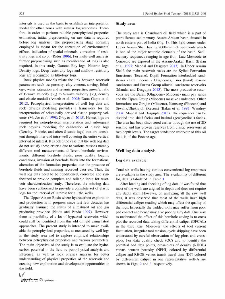
The study area is Chandmari oil field which is a part of

petroliferous sedimentary Assam-Arakan basin situated in

north eastern part of India (Fig. 1). This field comes under

Upper Assam Shelf having 7000-m-thick sediments which

is one of the major tectonic elements of the basin. Sedi-

mentary sequences ranging in age from Late Mesozoic to

Cenozoic are exposed in the Assam-Arakan Basin (Balan

et al. 1997; Mandal and Dasgupta 2013). In Upper Assam

Shelf, the main reservoir rocks are the Sylhet Formation

limestones (Eocene), Kopili Formation interbedded sand-

stones (Late Eocene - Oligocene), Tura (basal) marine

sandstones and Surma Group alluvial sandstone reservoirs

(Mandal and Dasgupta 2013). The most productive reser-

voirs are the Barail (Oligocene- Miocene) main pay sands

and the Tipam Group (Miocene) massive sandstones. Other

formations are Girujan (Miocene), Namsang (Pliocene) and

Siwalik/Dhekiajuli (Recent) (Balan et al. 1997; Wandrey

2004; Mandal and Dasgupta 2013). The sequences can be

divided into shelf facies and basinal (geosynclinal) facies.

The area has been discovered earlier through the use of 2D

seismic and has proven reserves from clastic reservoirs at

two depth levels. The target sandstone reservoir of this oil

field is of the Eocene age.

Well log data analysis

Log data available

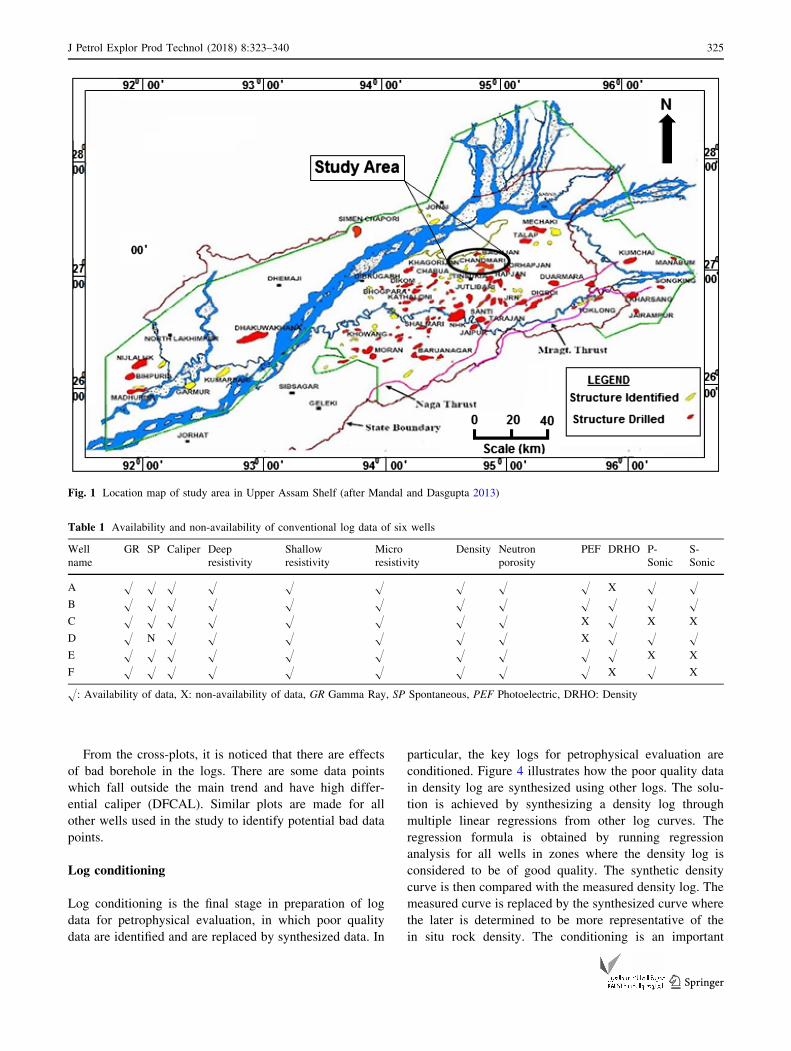
Total six wells having various conventional log responses

are available in the study area. The availability of different

log data is tabulated in Table 1.

After loading and checking of log data, it was found that

most of the wells are aligned in depth and does not require

any depth shift. However, on analyzing all the raw well

data, it was observed that most of the wells have high

differential caliper reading which may affect the quality of

the logs. Especially the padded tools may suffer from poor

pad contact and hence may give poor quality data. One way

to understand the effect of this borehole caving is to cross

plot the recorded data taking differential caliper (DFCAL)

in the third axis. Moreover, the effects of tool current

fluctuation, irregular tool tension, cycle skipping have been

understood by careful observation of log plots and cross-

plots. For data quality check (QC) and to identify the

potential bad data points, cross-plots of density (RHOB)

versus neutron porosity (NPHI) colored by differential

caliper and RHOB versus transit travel time (DT) colored

by differential caliper in one representative well-A are

shown in Figs. 2 and 3, respectively.

324 J Petrol Explor Prod Technol (2018) 8:323–340

123

From the cross-plots, it is noticed that there are effects

of bad borehole in the logs. There are some data points

which fall outside the main trend and have high differ-

ential caliper (DFCAL). Similar plots are made for all

other wells used in the study to identify potential bad data

points.

Log conditioning

Log conditioning is the final stage in preparation of log

data for petrophysical evaluation, in which poor quality

data are identified and are replaced by synthesized data. In

particular, the key logs for petrophysical evaluation are

conditioned. Figure 4 illustrates how the poor quality data

in density log are synthesized using other logs. The solu-

tion is achieved by synthesizing a density log through

multiple linear regressions from other log curves. The

regression formula is obtained by running regression

analysis for all wells in zones where the density log is

considered to be of good quality. The synthetic density

curve is then compared with the measured density log. The

measured curve is replaced by the synthesized curve where

the later is determined to be more representative of the

in situ rock density. The conditioning is an important

Fig. 1 Location map of study area in Upper Assam Shelf (after Mandal and Dasgupta 2013)

Table 1 Availability and non-availability of conventional log data of six wells

Well

name

GR SP Caliper Deep

resistivity

Shallow

resistivity

Micro

resistivity

Density Neutron

porosity

PEF DRHO P-

Sonic

S-

Sonic

A H H H H H H H H H X H H

B H H H H H H H H H H H H

C H H H H H H H H X H X X

D H N H H H H H H X H H H

E H H H H H H H H H H X X

F H H H H H H H H H X H X

H: Availability of data, X: non-availability of data, GR Gamma Ray, SP Spontaneous, PEF Photoelectric, DRHO: Density

J Petrol Explor Prod Technol (2018) 8:323–340 325

123

process as the derived porosity and volume of clay as well

as the rock physics analysis is strongly dependent on the

density log. Several iterations are required to produce a log

that is consistent with rock physics model and sonic log

data. The process of density conditioning is illustrated

below for a representative well-A.

Fig. 2 RHOB versus NPHI cross-plot colored by differential caliper (data falling within the marked circle represent bad data)

Fig. 3 Cross-plot between RHOB and DT colored by differential caliper (data falling within the marked circle represent erroneous data)


123

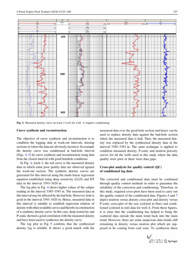
Curve synthesis and reconstruction

The objective of curve synthesis and reconstruction is to

condition the logging data at wash-out intervals, missing

sections or where the data are obviously incorrect. In example

the density curve was conditioned at bad-hole interval

(Figs. 4, 5) by curve synthesis and reconstruction using data

from the closest interval with good borehole conditions.

In Fig. 4, track-3, the red curve is the measured density

data in which some poor quality data are observed against

the wash-out section. The synthetic density curves are

generated for this interval using the multi-linear regression

equation established using deep resistivity (LLD) and DT

data in the interval 3393–3420 m.

The log plot in Fig. 4 shows higher values of the caliper

reading in the interval 3385–3393 m. The measured data in

this intervalmay be affected by the bad hole. However, hole is

good in the interval 3393–3420 m. Hence, measured data in

this interval is suitable to establish regression relation of

densitywith other available curves and thereby inconstruction

of a synthetic density curve. In this case, deep resistivity and

P-sonic showed a good correlation with the measured density

and have been used to synthesize the density curve.

The log plot in Fig. 5 confirms that the synthesized

density log is reliable. It shows a good match with the

measured data over the good-hole section and hence can be

used to replace density data against the bad-hole section

where the measured data is bad. Thus, the measured den-

sity was replaced by the synthesized density data in the

interval 3385–3393 m. The same technique is applied to

condition measured density, P-sonic and neutron porosity

curves for all the wells used in this study where the data

quality were poor or there were data gaps.

Cross-plot analysis for quality control (QC)

of conditioned log data

The corrected and conditioned data must be confirmed

through quality control methods in order to guarantee the

reliability of the correction and conditioning. Therefore, in

this study, required cross-plots have been used to carry out

the quality control of the conditioned data. Figures 6 and 7

depict neutron versus density cross-plot and density versus

P-sonic cross-plot of the raw (colored in blue) and condi-

tioned (colored in red) data for well-A. From these figures,

it is clear that the conditioning has helped to bring the

scattered data outside the main trend back into the main

trend. However, there are some suspicious data trends still

remaining in density versus neutron plot which are sup-

posed to be coming from coal zone. To synthesize these

Fig. 4 Measured density curve on track-3 (red) for well- A requires conditioning


123

data, there should be some good quality data available from

a similar coal zone in and around the bad data zone. In this

case there is no such zone available and hence for this zone

curve synthesis was not possible.

Another important criterion for rock physics modeling is

that input well data has to be consistent from well to well

unless there is significant geological variation. Since,

without consistent input log data, it is not possible to

Fig. 5 Well A-synthesized density curve (black) on top of measured density curve

Fig. 6 Well A is conditioned by RHOB and NPHI (red) on top of measured RHOB-NPHI (blue)


123

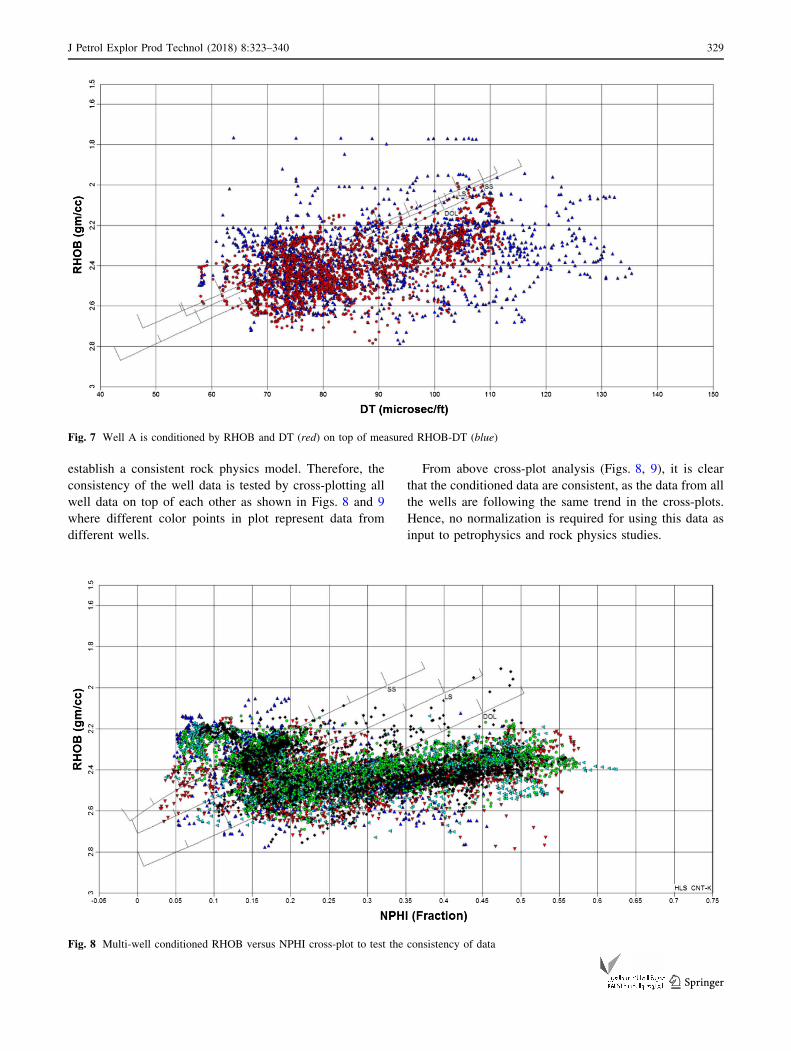
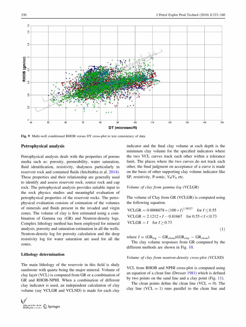
establish a consistent rock physics model. Therefore, the

consistency of the well data is tested by cross-plotting all

well data on top of each other as shown in Figs. 8 and 9

where different color points in plot represent data from

different wells.

From above cross-plot analysis (Figs. 8, 9), it is clear

that the conditioned data are consistent, as the data from all

the wells are following the same trend in the cross-plots.

Hence, no normalization is required for using this data as

input to petrophysics and rock physics studies.

Fig. 7 Well A is conditioned by RHOB and DT (red) on top of measured RHOB-DT (blue)

Fig. 8 Multi-well conditioned RHOB versus NPHI cross-plot to test the consistency of data


123

Petrophysical analysis

Petrophysical analysis deals with the properties of porous

media such as: porosity, permeability, water saturation,

fluid identification, resistivity, shalyness particularly in

reservoir rock and contained fluids (Inichinbia et al. 2014).

These properties and their relationship are generally used

to identify and assess reservoir rock, source rock and cap

rock. The petrophysical analysis provides suitable input to

the rock physics studies and meaningful evaluation of

petrophysical properties of the reservoir rocks. The petro-

physical evaluation consists of estimation of the volumes

of minerals and fluids present in the invaded and virgin

zones. The volume of clay is first estimated using a com-

bination of Gamma ray (GR) and Neutron-density logs.

Complex lithology method has been employed for mineral

analysis, porosity and saturation estimation in all the wells.

Neutron-density log for porosity calculation and the deep

resistivity log for water saturation are used for all the

zones.

Lithology determination

The main lithology of the reservoir in this field is shaly

sandstone with quartz being the major mineral. Volume of

clay layer (VCL) is computed from GR or a combination of

GR and RHOB-NPHI. When a combination of different

clay indicator is used, an independent calculation of clay

volume (say VCLGR and VCLND) is made for each clay

indicator and the final clay volume at each depth is the

minimum clay volume for the specified indicators where

the two VCL curves track each other within a tolerance

limit. The places where the two curves do not track each

other, the final judgment on acceptance of a curve is made

on the basis of other supporting clay volume indicator like

SP, resistivity, P-sonic, VP/VS etc.

Volume of clay from gamma log (VCLGR)

The volume of Clay from GR (VCLGR) is computed using

the following equation.

VCLGR ¼ 0:0006078 � ð100 � IÞ1:58527 for I� 0:55

VCLGR ¼ 2:1212 � I � 0:81667 for 0:55\I\0:73

VCLGR ¼ I for I� 0:73

ð1Þ

where I = (GRlog - GRclean)/(GRclay - GRclean).

The clay volume responses from GR computed by the

different methods are shown in Fig. 10.

Volume of clay from neutron-density cross-plot (VCLND)

VCL from RHOB and NPHI cross-plot is computed using

an equation of a clean line (Dresser 1981) which is defined

by two points on the sand line and a clay point (Fig. 11).

The clean points define the clean line (VCL = 0). The

clay line (VCL = 1) runs parallel to the clean line and

Fig. 9 Multi-well conditioned RHOB versus DT cross-plot to test consistency of data


123

passes through the clay point. Lines of constant VCL run

parallel to those lines at a position proportional to the

relative distance between the clean and clay lines, as shown

in Fig. 11. The ‘end points’ in density, neutron and gamma

ray for wet clay are chosen such that the volume of wet

clay is estimated to be around 70–75% against shale sec-

tion. On the basis of available data, petrophysical analysis

and rock physics modeling, the VCL from neutron-density

cross-plot and GR allowed the identification of reservoir

rock and non-reservoir rock more clearly in most of the

zones and provided greater consistency between the

petrophysical and rock physics models.

Computation of PHIE and water saturation (Sw)

by complex lithology model

Porosity is calculated with the ‘Multimin’ method using the

density and neutron logs. The clay end points used for

porosity calculation are the same as the end points used in

VCL calculations. Figure 12 shows the rock model based

on the ‘effective porosity and wet clay.’

The effective porosity is computed from neutron-density

cross-plot (Bateman 1985).

/e ¼/D � /Nsh

� /N � /Dsh

/Nsh� /Dsh

ð2Þ

where /e is the effective porosity, /D is the density

porosity, /Nshis neutron porosity of shale, /N is neutron

porosity, /Dshis the density porosity of shale.

The porosities /D and /N in Eq. (2) have been corrected

for the effect of residual hydrocarbon before dealing with

the equations.

The density derived porosity /D is corrected using the

residual hydrocarbons by the formula,

/D ¼ dma � dþ 1:07Rmf

Rxo

� �1=2

1:11� 1:24dhð Þ" #,

dma � 1þ 1:07 1:11� 1:24dhð Þf gð3Þ

where dma is matrix density, d is the log reading, dh is thehydrocarbon density, Rmf is the mud filtrate resistivity, Rxo

is the flushed zone resistivity, and /D is the residual

hydrocarbon corrected porosity (Schlumberger 1967).

The neutron derived porosity /N is corrected using the

residual hydrocarbon by the formula

/N ¼/na= 1� Shrð Þ dmf 1�Pð Þ� dh� 0:3ð Þ=dmf 1�Pð Þf g½ �ð4Þ

where /na is the apparent neutron porosity, P is the mud

filtrate salinity (106 ppm), and /N is the neutron porosity

corrected from hydrocarbon effect (Dresser 1981).

Water saturation in shaly sand is determined using

Poupon–Leveaux Indonesian model (Poupon and Leveaux

1971). Indonesian equation is defined as

Fig. 10 VCL responses from GR computed by different methods

Fig. 11 Schematic diagram of volume of clay from density and

neutron cross-plot

Wet ClayMatrix Effec�ve Porosity

Fig. 12 The display of ‘effective porosity and wet clay’ model


123

1

Rt

¼ SnwV2�Vsh

sh

Rsh

� �1=2

þ /me

Rw

� �1=2" #2

ð5Þ

Sw ¼ V2�Vsh

sh

Rsh

� �1=2

þ /me

Rw

� �1=2" #2

Rt

8<:

9=;

�1=n

ð6Þ

where /e = Effective porosity, Vsh = Shale volume,

Rsh = Resistivity of shale, Rw = Water resistivity, Rt =

Deep resistivity, Sw = Water saturation.

The clay end points used for porosity calculation are the

same as the end points used in VCL calculations. For

iterative hydrocarbon correction, residual hydrocarbon

saturation Srh is derived from Sxo or from an empirical

equation that uses Sw.

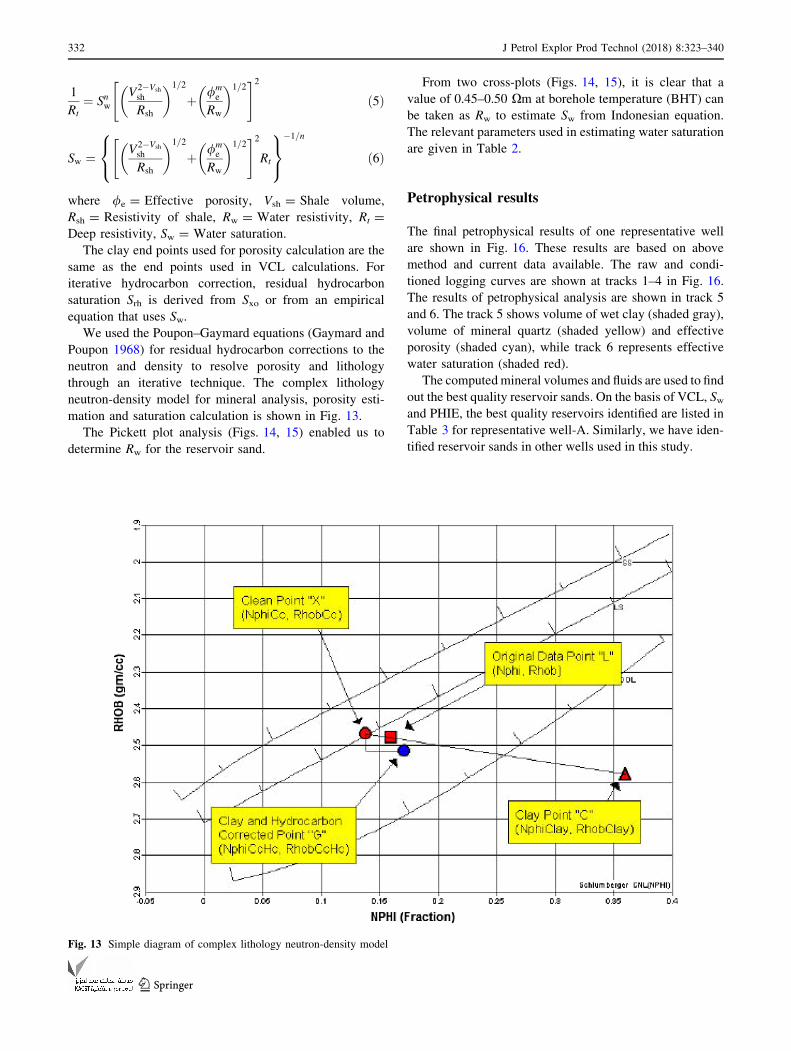
We used the Poupon–Gaymard equations (Gaymard and

Poupon 1968) for residual hydrocarbon corrections to the

neutron and density to resolve porosity and lithology

through an iterative technique. The complex lithology

neutron-density model for mineral analysis, porosity esti-

mation and saturation calculation is shown in Fig. 13.

The Pickett plot analysis (Figs. 14, 15) enabled us to

determine Rw for the reservoir sand.

From two cross-plots (Figs. 14, 15), it is clear that a

value of 0.45–0.50 Xm at borehole temperature (BHT) can

be taken as Rw to estimate Sw from Indonesian equation.

The relevant parameters used in estimating water saturation

are given in Table 2.

Petrophysical results

The final petrophysical results of one representative well

are shown in Fig. 16. These results are based on above

method and current data available. The raw and condi-

tioned logging curves are shown at tracks 1–4 in Fig. 16.

The results of petrophysical analysis are shown in track 5

and 6. The track 5 shows volume of wet clay (shaded gray),

volume of mineral quartz (shaded yellow) and effective

porosity (shaded cyan), while track 6 represents effective

water saturation (shaded red).

The computedmineral volumes and fluids are used to find

out the best quality reservoir sands. On the basis of VCL, Swand PHIE, the best quality reservoirs identified are listed in

Table 3 for representative well-A. Similarly, we have iden-

tified reservoir sands in other wells used in this study.

Fig. 13 Simple diagram of complex lithology neutron-density model


123

Rock physics modeling

The rock physics studies have allowed combining elastic

properties of minerals and fluids that predict the measured

elastic logs of the rocks: density, P-velocity and S-velocity

(Avseth et al. 2005; Xin and Han 2009). The analysis

confirms that the rock physics model devised for these logs

is appropriate to explain the rock behavior, understand the

relationships between the petrophysical and elastic rock

properties and it could synthesize good quality P-sonic and

Fig. 14 Multi-well Pickett plot between PHID (density porosity) and LLD (deep resistivity) for determining Rw

Fig. 15 Multi-well GR versus RWA plot to determine Rw


123

S-sonic log where no recorded sonic logs were available

(Mavko and Mukerji 1995; Avseth et al. 2006).

The modeling was started with a shale density of

2.8 g/cc. This led to a systematic error in P-wave

velocity. This error was fed back to find the best effec-

tive clay density to obtain a good fit to the P-velocity. A

plot of clay density versus depth gave a systematic

variation, and a curve was fitted for the interval below

Lk ? Th. These curves were then used as clay density.

The aspect ratio of clean and S-velocity of clay were

then optimized to fit the data with measured shear wave

velocity. Thereafter, VP/VS of clay was adjusted to

optimize the fit to the measured P-velocity. The model in

this case is based on the volume of clay and saturation

derived from the petrophysics and the total porosity

derived from the density. The derivation of model

involved mixing of minerals and pore space, then the

fluids and finally the fluid mixture is introduced into the

porous mineral mix via Gassmann’s equations (Batzle

and Wang 1992; Mavko and Mukerji 1995; Mavko et al.

1998; Berryman 1999; Han and Batzle 2004). The

modeling started under the assumption that the measured

data are representative of invaded formation. The satu-

ration is set to SW0.2 to model the invaded zone for all the

wells. Other fluids can also be introduced to understand

the sensitivity of the rock properties to the fluid type.

Table 2 Parameters used for determining water saturation

Parameter Value

RW 0.45–0.50 Xm @BHT

m 1.85

n 2

a 0.9

Rtcl 5 Xm

Rxocl 5 Xm

Fig. 16 Petrophysical results of one representative well-A

Table 3 Reservoir parameters estimated for representative well-A

Interval (m) VCL (%) Sw (%) PHIE (%)

3926.3–3927.4 15–20 28 20

3901.4–3905.6 5–15 19–25 20–35

3848–3850.4 5–10 20–22 35


123

Mineral mixing

The minerals and pore spaces are mixed using the self-

consistent method (Berryman 1980). In Berryman self-

consistent method, the pore space is modeled as ellipsoids

with an assigned aspect ratio which is dependent on the

mineral with which the pore space is associated. The

minerals are also modeled as ellipsoids and assigned the

same aspect ratio as their associated pores. The rock/fluid

properties which are used to model the sand shale

sequences using the self-consistent method are summarized

in Table 4.

Fluid mixing

The fluids, brine and hydrocarbon are mixed to produce

effective properties that can be used in Gassmann model-

ing. The density mix is straightforward using the volume

Table 4 Rock properties for different lithology and fluid used to model the sand/shale sequences

Density (kg/m3) P-velocity (m/s) S-velocity (m/s) Aspect ratio

Grain 2650 6200 3800 Varied with porosity

Dry clay Varied with depth Varied with depth Varied with depth Varied with porosity

Brine 1109 1691.5 n/a

Gas 220 591 n/a

Live oil 776 1037 n/a

Fig. 17 A comparison of rock physics modeled log with measured log for one representative well-A


123

average of the densities of different fluids present. The

acoustic properties are mixed using Brie’s formula (Brie

et al. 1995) to account for the variation in distribution of

the different fluids within the pore space,

kfl ¼ kbr � kg� �

Sew þ kg ð7Þ

where kfi is the effective acoustic modulus of the fluid

mixture, kbr is the acoustic modulus of brine, kg is the

acoustic modulus of gas (or oil) and Sw is the brine satu-

ration. The exponent ‘e’ can vary from 1 to infinity, where

1 represents a complete mixing of the fluids. A value of

e = 3 is mainly used in the current modeling.

Mineral and fluid mixing

Gassmann (1951a, b) equation is used to model the effect

of the fluids in the pore spaces (Biot 1956). The fluids are

initially incorporated with the mixture that represents sat-

urations in the invaded zones as seen by the log. Various

versions of the fluid substituted logs (all brine, all gas, and

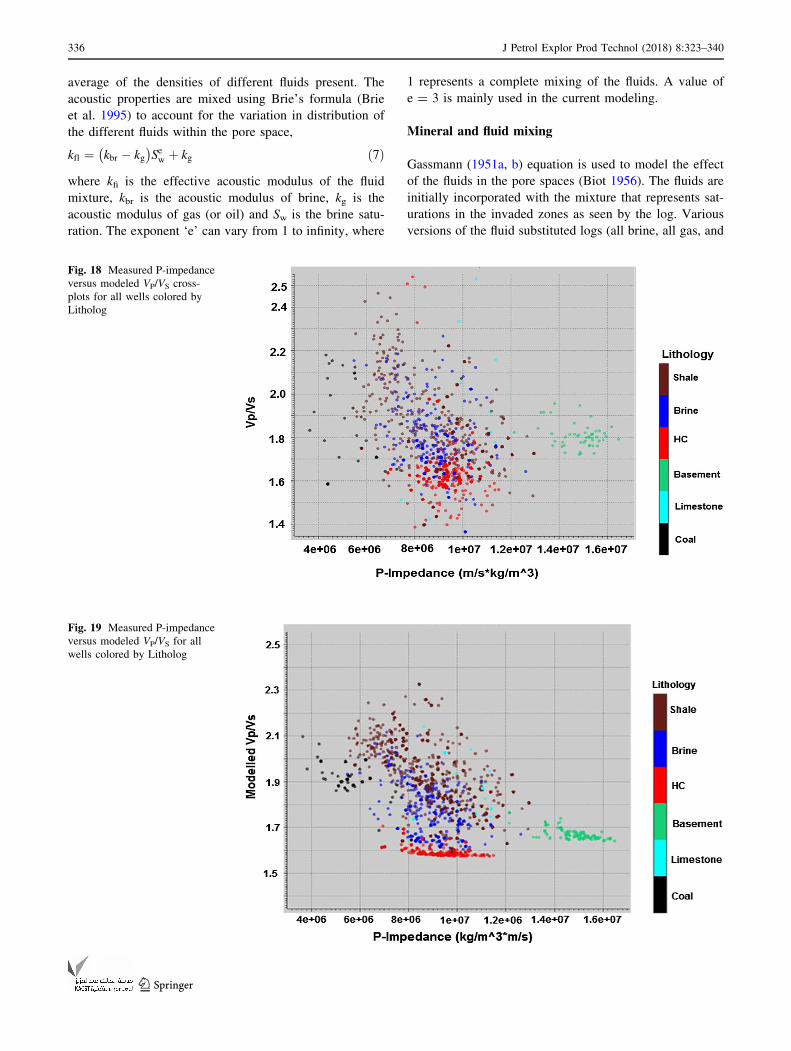
Fig. 18 Measured P-impedance

versus modeled VP/VS cross-

plots for all wells colored by

Litholog


versus modeled VP/VS for all

wells colored by Litholog


123

all oil) are generated. The quality of the model is assessed

by comparing the modeled and measured log data as shown

in Fig. 17. In Fig. 17, the modeled density, P-velocity,

S-velocity and VP/VS colored in red are plotted in the first

four tracks on top of the measured curves colored in blue.

Track 5, 6 and 7 represent total porosity, Vclay and Sw. The

plots indicate that there is good correlation between the

modeled logs and measured logs data. However, the

modeled S-sonic log shows some deviations with the

measured log data at several places because measured

S-sonic log is affected by bore hole caving which might

have caused abrupt variations in the log. There are some

spikes and missing data observed in the measured logs

which have also been taken care of by the rock physics

model. The model could also rectify the sonic data where

the measured data may have not been processed properly.

The final modeled elastic logs also allow one to

understand the relationship between the petrophysical and


versus effective porosity for all



versus total porosity for all the



123

elastic rock properties which can be used further to predict

the reservoir properties away from the well locations.

Figures 18 and 19 show cross-plots of measured and

modeled P-impedance versus VP/VS colored by Lithologs

for all the wells, respectively. Some of the relations of the

reservoir properties are tested by cross-plotting P-impe-

dance versus effective and total porosity, P-impedance

versus density as shown in Figs. 20, 21 and 22. Different

Lithologies, e.g. shale, hydrocarbon, coal, and basement

etc., show good separation of properties in P-impedance

versus VP/VS domain.

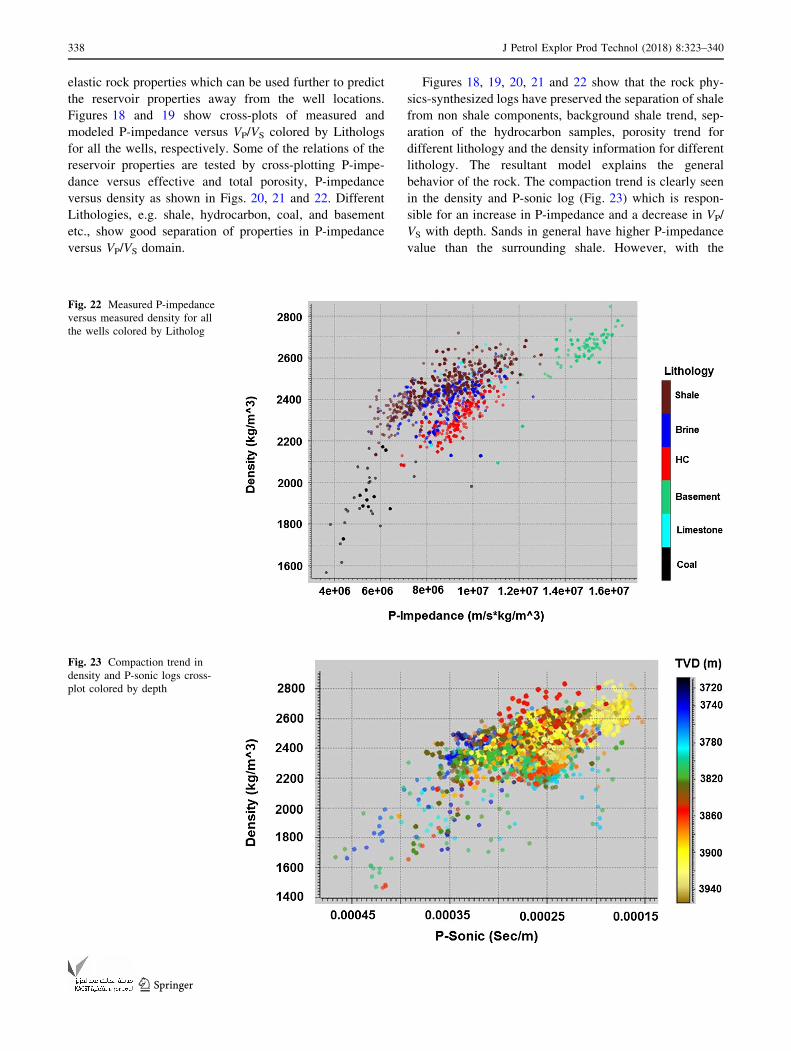
Figures 18, 19, 20, 21 and 22 show that the rock phy-

sics-synthesized logs have preserved the separation of shale

from non shale components, background shale trend, sep-

aration of the hydrocarbon samples, porosity trend for

different lithology and the density information for different

lithology. The resultant model explains the general

behavior of the rock. The compaction trend is clearly seen

in the density and P-sonic log (Fig. 23) which is respon-

sible for an increase in P-impedance and a decrease in VP/

VS with depth. Sands in general have higher P-impedance

value than the surrounding shale. However, with the


versus measured density for all

the wells colored by Litholog

Fig. 23 Compaction trend in

density and P-sonic logs cross-

plot colored by depth


123

introduction of hydrocarbon, the impedance value decrea-

ses as expected.

Conclusions

A detailed petrophysical analysis blended with rock physics

modeling have been carried out for reservoir characteriza-

tion of Chandmari oilfield in Upper Assam-Arakan basin,

India, using a suite of well log data from six wells in the field.

Lithological interpretation and effects of rock minerals and

fluids have been assessed. The Eocene reservoirs are mainly

sandstone with inferred clay matrix up to 20% and some

calcareous cementation. Some of these reservoirs are very

clean with clay content as low as 5–10%. Sands are inter-

preted to be continuous inmost of the blocks. However, there

is some shale intercalations observed in many cases. A wide

range of variation is found in water saturation with lowest

value observed at 5%. The effective porosity for these sands

is varying in the range of 15–22% for most of the wells. The

effect of gas in the reservoir sands are very well understood

in the log response for most of the wells. Gas bearing zone

showed very big cross over for neutron-density curves and is

also supported by very high resistivity. However, it was

difficult to differentiate between oil and gas on the basis of

the measured logs.

Rock physics modeled elastic logs also allowed to

understand the relationship between the petrophysical and

elastic rock properties to be used for further prediction of

reservoir properties away from thewell locations. Themodel

explained the general behavior of the rock and synthesizes

the good quality P-sonic and S-sonic logs where no recorded

sonic data were available. Rock physics-synthesized logs

also preserved the porosity trend and density information for

different lithology. The compaction trend is clearly seen in

the density and P-sonic log which causes an increase in

P-impedance and decrease in VP/VS with depth.

Acknowledgements The authors are thankful to the Oil India Lim-

ited, Duliajan, Assam, for permitting to use the collected well log and

geological information for this study.

Open Access This article is distributed under the terms of the Crea-

tive Commons Attribution 4.0 International License (http://

creativecommons.org/licenses/by/4.0/), which permits unrestricted

use, distribution, and reproduction in any medium, provided you give

appropriate credit to the original author(s) and the source, provide a link

to the Creative Commons license, and indicate if changes were made.

References

Avseth P, Mukerji T, Mavko G (2005) Quantitative seismic

interpretation: applying rock physics to reduce interpretation

risk. Cambridge University Press, Cambridge, p 359

Avseth P, Mukherji T, Mavko G (2006) Quantitative seismic

interpretation. Cambridge University Press, Cambridge

Balan KC, Banerjee B, Pati LN, Shilpkar KB, Pandey MN, Sinha

MK, Zutshi PI (1997) Quantitative genetic modeling of Upper

Assam Shelf. In: Proceedings of second international petroleum

conference and exhibition, PETROTECH-97, New Delhi, vol 1,

pp 341–349

Bateman RM (1985) Open-hole log analysis and formation evaluation

Schlumberger Inc. In: Log interpretation principles. Schlum-

berger education services, Houston, USA

Batzle ML, Wang ZJ (1992) Seismic properties of pore fluids.

Geophysics 57:1396–1408

Berryman JG (1980) Long-wavelength propagation in composite

elastic media II ellipsoidal inclusions. J Acoust Soc Am

68:1820–1831

Berryman JG (1999) Origin of Gassmann’s equations. Geophysics

64:1627–1629

Biot MA (1956) Theory of propagation of elastic waves in a fluid-

saturated porous solid. J Acoust Soc Am 28:168–191

Brie A, Pampuri F, Marsala AF, Meazza O (1995) Shear sonic

interpretation in gas-bearing sands. Soc Pet Explor (SPE)

30595:701–710

Chang HC, Kopaska-Merkel DC, Chen HC (2002) Identification of

lithofacies using Kohonen self organizing maps. Comput Geosci

28:223–229

Datta Gupta S, Chatterjee R, Farooqui MY (2012) Rock physics

template (RPT) analysis of well logs and seismic data for

lithology and fluid classification in Cambay basin. Int J Earth Sci

101(5):1407–1426

Dresser A (1981) Well logging and interpretation techniques. Dresser

Industries Inc., Addison

Ellis DV (1987) Well logging for earth scientists. Elsevier, New York

Gassmann F (1951a) Elastic waves through a packing of spheres.

Geophysics 16:673–685

Gassmann F (1951b) Elasticity of porous media. Uberdie elastizitat-

porosermedien, Vierteljahrsschrift der NaturforschendenGes-

selschaft 96:1–23

Gaymard R, Poupon A (1968) Response of neutron and formation

density logs in hydrocarbon bearing formations. Log Anal

9(5):3–12

Gray D, Day S, Schapper S (2015) Rock physics driven seismic data

processing for the Athabasca oil sands, Northeastern Alberta.

CSEG Recorder March, pp 32–40

Han D, Batzle ML (2004) Gassmann’s equation and fluid-saturation

effects on seismic velocities. Geophysics 69:398–405

Inichinbia S, Sule PO, Ahmed AL, Hamaza H, Lawal KM (2014)

Petro physical analysis of among hydrocarbon field fluid and

lithofacies using well log data. IOSR J Appl Geol Geophys

2:86–96

Ishwar NB, Bhardwaj A (2013) Petrophysical well log analysis for

hydrocarbon exploration in parts of Assam-Arakan basin, India.

In: 10th Biennial international conference and exposition,

society of exploration geophysicists, Kochi, India, p 153

Joshi GK, Shyammohan V, Reddy AS, Singh B, Chandra M (2004)

Reservoir characterization through log property mapping in

Geleki field of upper Assam, India. In: 5th Conference and

exposition on petroleum geophysics, Hyderabad, India,

pp 685–687

Mandal KL, Dasgupta R (2013) Upper Assam basin and its basinal

depositional history. In: 10th Biennial international conference

and exposition, society of petroleum geophysicists, Kochi, p 292

Mavko G, Mukerji T (1995) Seismic pore space compressibility and

Gassmann’s relation. Geophysics 60(6):1743–1749

Mavko G, Mukerji T, Dvorkin J (1998) The rock physics handbook:

tools for seismic analysis of porous media. Cambridge Univer-

sity Press, Cambridge


123

http://creativecommons.org/licenses/by/4.0/

http://creativecommons.org/licenses/by/4.0/

Mukerji T, Avseth P, Mavko G, Takahashi I, Gonzalez EF (2001)

Statistical rock physics: combining rock physics, information

theory, and geostatistics to reduce uncertainty in seismic

reservoir characterization. Lead Edge 20(3):313–319. doi:10.

1190/1.1438938

Naidu BD, Panda BK (1997) Regional source rock mapping in Upper

Assam Shelf. In: Proceedings of the second international

petroleum conference and exhibition (PETROTECH-97), New

Delhi, vol 1, pp 350–364

Neog PK, Borah NM (2000) Reservoir characterization through well

test analysis assists in reservoir simulation—a case study. In:

SPE Asia Pacific oil and gas conference and exhibition,

Brisbane, Australia, 16–18 October

Poupon A, Leveaux J (1971) Evaluation of water saturations in shaly

formations. Log Anal 12(4):3–8

Rider M (1996) The geological interpretation of well log, 2nd edn.

Whittles Publishing, London. ISBN-13: 978-0954190606

Sarasty JJ, Stewart RR (2003) Analysis of well-log data from the

White Rose oilfield, offshore Newfoundland. CREWES Res Rep

15:1–16

Schlumberger (1967) Well evaluation conference Middle East, vol 1,

Text vol 2, Examples 2. Schlumberger, Paris, France

Wandrey CJ (2004) Sylhet-Kopili/Barail-Tipam composite total

petroleum system, Assam geological province, India. USGS

Open File Report 2208-D

Xin G, Han D (2009) Lithology and fluid differentiation using rock

physics templates. Lead Edge 28:60–65


123

http://dx.doi.org/10.1190/1.1438938

http://dx.doi.org/10.1190/1.1438938

petrophysical evaluation of well log data and rock physics ... · keywords petrophysics rock...

Documents