PHASE RETRIEVAL FOR IMAGING PROBLEMS.

FAJWEL FOGEL, IRENE WALDSPURGER, AND ALEXANDRE D’ASPREMONT

ABSTRACT. We study convex relaxation algorithms for phase retrieval on imaging problems. We show thatexploiting structural assumptions on the signal and the observations, such as sparsity, smoothness or positivity,can significantly speed-up convergence and improve recovery performance. We detail numerical results inmolecular imaging experiments simulated using data from the Protein Data Bank (PDB).

1. INTRODUCTION

Phase retrieval seeks to reconstruct a complex signal, given a number of observations on the magnitudeof linear measurements, i.e. solve

find xsuch that |Ax| = b

(1)

in the variable x ∈ Cp, where A ∈ Rn×p and b ∈ Rn. This problem has direct applications in X-rayand crystallography imaging, diffraction imaging, Fourier optics or microscopy for example, in problemswhere physical limitations mean detectors usually capture the intensity of observations but cannot recovertheir phase. In what follows, we will focus on problems arising in diffraction imaging, where A is usuallya Fourier transform, often composed with one or multiple masks (a technique sometimes called ptychogra-phy). The Fourier structure, through the FFT, considerably speeds up basic linear operations, which allowsus to solve large scale convex relaxations on realistically large imaging problems. We will also observe thatin many of the imaging problems we consider, the Fourier transform is very sparse, with known support (welose the phase but observe the magnitude of Fourier coefficients), which allows us to considerably reducethe size of our convex phase retrieval relaxations.

Because the phase constraint |Ax| = b is nonconvex, the phase recovery problem (1) is non-convex.Several greedy algorithms have been developed (see [Gerchberg and Saxton, 1972; Fienup, 1982; Griffinand Lim, 1984; Bauschke et al., 2002] among others), which alternate projections on the range of A andon the nonconvex set of vectors y such that |y| = |Ax|. While empirical performance is often good,these algorithms can stall in local minima. A convex relaxation was introduced in [Chai et al., 2011] and[Candes et al., 2011] (who call it PhaseLift) by observing that |Ax|2 is a linear function of X = xx∗

which is a rank one Hermitian matrix, using the classical lifting argument for nonconvex quadratic programsdeveloped in [Shor, 1987; Lovasz and Schrijver, 1991]. The recovery of x is thus expressed as a rankminimization problem over positive semidefinite Hermitian matrices X satisfying some linear conditions,i.e. a matrix completion problem. This last problem has received a significant amount of attention becauseof its link to compressed sensing and the NETFLIX collaborative filtering problem. This minimum rankmatrix completion problem is approximated by a semidefinite program which has been shown to recover xfor several (random) classes of observation operators A [Candes et al., 2011, 2013a,b].

On the algorithmic side, [Waldspurger et al., 2012] showed that the phase retrieval problem (1) canbe reformulated in terms of a single phase variable, which can be read as an extension of the MAXCUTcombinatorial graph partitioning problem over the unit complex torus, allowing fast algorithms designed forsolving semidefinite relaxations of MAXCUT to be applied to the phase retrieval problem.

Date: April 8, 2014.2010 Mathematics Subject Classification. 94A12, 90C22, 90C27.Key words and phrases. Phase recovery, semidefinite programming, X-ray diffraction, molecular imaging, Fourier optics.

1

On the experimental side, phase recovery is a classical problem in Fourier optics for example [Goodman,2008], where a diffraction medium takes the place of a lens. This has a direct applications in X-ray andcrystallography imaging, diffraction imaging or microscopy [Harrison, 1993; Bunk et al., 2007; Johnsonet al., 2008; Miao et al., 2008; Dierolf et al., 2010].

Here, we implement and study several efficient convex relaxation algorithms for phase retrieval on imag-ing problem instances whereA is based on a Fourier operator. We show in particular how structural assump-tions on the signal and the observations (e.g. sparsity, smoothness, positivity, known support, oversampling,etc.) can be exploited to both speed-up convergence and improve recovery performance. While no experi-mental data is available from diffraction imaging problems with multiple randomly coded illuminations, wesimulate numerical experiments of this type using molecular density information from the protein data bank[Berman et al., 2002]. Our results show in particular that the convex relaxation is stable and that in somesettings, as few as two random illuminations suffice to reconstruct the image.

The paper is organized as follows. Section 2 briefly recalls the structure of some key algorithms usedin phase retrieval. Section 3 describes applications to imaging problems and how structural assumptionscan sifnificantly reduce the cost of solving large-scale instances and improve recovery performance. Sec-tion 4 details some numerical experiments while Section 5 describes the interface to the numerical librarydeveloped for these problems.

Notations. We write Sp (resp. Hp) the cone of symmetric (resp. Hermitian) matrices of dimension p ; S+p

(resp. H+p ) denotes the set of positive symmetric (resp. Hermitian) matrices. We write ‖ · ‖p the Schatten p-

norm of a matrix, that is the p-norm of the vector of its eigenvalues (in particular, ‖·‖∞ is the spectral norm).We writeA† the (Moore-Penrose) pseudoinverse of a matrixA, andA◦B the Hadamard (or componentwise)product of the matrices A and B. For x ∈ Rp, we write diag(x) the matrix with diagonal x. When X ∈ Hp

however, diag(X) is the vector containing the diagonal elements of X . For X ∈ Hp, X∗ is the Hermitiantranspose of X , with X∗ = (X)T . Finally, we write b2 the vector with components b2i , i = 1, . . . , n.

2. ALGORITHMS

In this section, we briefly recall several basic algorithmic approaches to solve the phase retrieval prob-lem (1). Early methods were all based on extensions of an alternating projection algorithm. However,recent results showed that phase retrieval could be interpreted as a matrix completion problem similar to theNETFLIX problem, a formulation which yields both efficient convex relaxations and recovery guarantees.

2.1. Greedy algorithms. The phase retrieval problem (1) can be rewritten

minimize ‖Ax− y‖22subject to |y| = b

(2)

where we now optimize over both phased observations y ∈ Cn and signal x ∈ Cp. Several greedy algorithmsattempt to solve this problem using variants of alternating projections, one iteration minimizing the quadraticerror (the objective of (2)), the next normalizing the moduli (to satisfy the constraint). We detail some of themost classical examples in the paragraphs that follow.

The algorithm Gerchberg-Saxton by [Gerchberg and Saxton, 1972] for instance seeks to reconstruct y =Ax and alternates between orthogonal projections on the range of A and normalization of the magnitudes|y| to match the observations b. The cost per iteration of this method is minimal but convergence (when ithappens) is often slow.

A classical “input-output” variant, detailed here as algorithm Fienup, introduced by [Fienup, 1982] addsan extra penalization step which usually speeds up convergence and improves recovery performance whenadditional information is available on the support of the signal. Oversampling the Fourier transform formingA in imaging problems usually helps performance as well. Of course, in all these cases, convergence to aglobal optimum cannot be guaranteed but empirical recovery performance is often quite good.

2

Algorithm 1 Gerchberg-Saxton.

Input: An initial y1 ∈ F, i.e. such that |y1| = b.1: for k = 1, . . . , N − 1 do2: Set

yk+1i = bi

(AA†yk)i|(AA†yk)i|

, i = 1, . . . , n. (Gerchberg-Saxton)

3: end forOutput: yN ∈ F.

Algorithm 2 Fienup

Input: An initial y1 ∈ F, i.e. such that |y1| = b, a parameter β > 0.1: for k = 1, . . . , N − 1 do2: Set

wi =(AA†yk)i|(AA†yk)i|

, i = 1, . . . , n.

3: Setyk+1i = yki − β(yki − biwi) (Fienup)

4: end forOutput: yN ∈ F.

2.2. PhaseLift: semidefinite relaxation in signal. Using a classical lifting argument by [Shor, 1987], andwriting

|a∗ix|2 = b2i ⇐⇒ Tr(aia∗ixx

∗) = b2i[Chai et al., 2011; Candes et al., 2011] reformulate the phase recovery problem (1) as a matrix completionproblem, written

minimize Rank(X)subject to Tr(aia

∗iX) = b2i , i = 1, . . . , n

X � 0

in the variable X ∈ Hp, where X = xx∗ when exact recovery occurs. This last problem can be relaxed as

minimize Tr(X)subject to Tr(aia

∗iX) = b2i , i = 1, . . . , n

X � 0(PhaseLift)

which is a semidefinite program (called PhaseLift by Candes et al. [2011]) in the variable X ∈ Hp. Thisproblem is solved in [Candes et al., 2011] using first order algorithms implemented in [Becker et al., 2011].This semidefinite relaxation has been shown to recover the true signal x exactly for several classes of obser-vation operators A [Candes et al., 2011, 2013a,b].

2.3. PhaseCut: semidefinite relaxation in phase. As in [Waldspurger et al., 2012] we can rewrite thephase reconstruction problem (1) in terms of a phase variable u (such that |u| = 1) instead of the signal x.In the noiseless case, we then write the constraint |Ax| = b as Ax = diag(b)u, where u ∈ Cn is a phasevector, satisfying |ui| = 1 for i = 1, . . . , n, so problem (1) becomes

minimize ‖Ax− diag(b)u‖22subject to |ui| = 1

(3)

where we optimize over both phase u ∈ Cn and signal x ∈ Cp. While the objective of this last problem isjointly convex in (x, u), the phase constraint |ui| = 1 is not.

3

Now, given the phase, signal reconstruction is a simple least squares problem, i.e. given u we obtain x as

x = A† diag(b)u (4)

where A† is the pseudo inverse of A. Replacing x by its value in (3), the phase recovery problem becomes

minimize u∗Musubject to |ui| = 1, i = 1, . . . n,

(5)

in the variable u ∈ Cn, where the Hermitian matrix

M = diag(b)(I−AA†)diag(b)

is positive semidefinite. This problem is non-convex in the phase variable u. [Waldspurger et al., 2012]detailed greedy algorithm Greedy to locally optimize (5) in the phase variable.

Algorithm 3 Greedy algorithm in phase.

Input: An initial u ∈ Cn such that |ui| = 1, i = 1, . . . , n. An integer N > 1.1: for k = 1, . . . , N do2: for i = 1, . . . n do3: Set

ui =−∑

j 6=iMjiuj∣∣∣∑j 6=iMjiuj

∣∣∣ (Greedy)

4: end for5: end for

Output: u ∈ Cn such that |ui| = 1, i = 1, . . . , n.

A convex relaxation to (5) was also derived in [Waldspurger et al., 2012] using the classical lifting argumentfor nonconvex quadratic programs developed in [Shor, 1987; Lovasz and Schrijver, 1991]. This relaxationis written

min. Tr(UM)subject to diag(U) = 1, U � 0,

(PhaseCut)

which is a semidefinite program (SDP) in the matrix U ∈ Hn. This problem has a structure similar to theclassical MAXCUT relaxation and instances of reasonable size can be solved using specialized implemen-tations of interior point methods designed for that problem [Helmberg et al., 1996]. Larger instances aresolved in [Waldspurger et al., 2012] using the block-coordinate descent algorithm BlockPhaseCut.

Ultimately, algorithmic choices heavily depend on problem structure, and these will be discussed in detailin the section that follows. In particular, we will study how to exploit structural information on the signal(nonnegativity, sparse 2D FFT, etc.), to solve realistically large instances formed in diffraction imagingapplications.

3. IMAGING PROBLEMS

In the imaging problems we study here, various illuminations of a single object are performed throughrandomly coded masks, hence the matrix A is usually formed using a combination of random masks andFourier transforms, and we have significant structural information on both the signal we seek to reconstruct(regularity, etc.) and the observations (power law decay in frequency domain, etc.). Many of these addi-tional structural hints can be used to speedup numerical operations, convergence and improve phase retrievalperformance. The paragraphs that follow explore these points in more detail.

4

Algorithm 4 Block Coordinate Descent Algorithm for PhaseCut.

Input: An initial U0 = In and ν > 0 (typically small). An integer N > 1.1: for k = 1, . . . , N do2: Pick i ∈ [1, n].3: Compute

u = Ukic,icMic,i and γ = u∗Mic,i (BlockPhaseCut)

4: If γ > 0, set

Uk+1ic,i = Uk+1∗

i,ic = −√

1− νγ

x

elseUk+1ic,i = Uk+1∗

i,ic = 0.

5: end forOutput: A matrix U � 0 with diag(U) = 1.

3.1. Fourier operators. In practical applications, because of the structure of the linear operator A, wemay often reduce numerical complexity, using the Fourier structure of A to speedup the single matrix-vector product in algorithm BlockPhaseCut. We detail the case where A corresponds to a Fourier transformcombined with k random masks, writing I1, ..., Ik ∈ Cp be the illumination masks. The image byA of somesignal x ∈ Cp is then

Ax =

F(I1 ◦ x)...

F(Ik ◦ x)

,

and the pseudo-inverse of A also has a simple structure, with

A†

(y1...yk

)=

k∑l=1

F−1(yl) ◦ I ′l

where I ′l is the dual filter of Il, which is

I ′l = I l/

(∑s

|Is|2).

With the fast Fourier transform, computing the image of a vector by A or A† only requires O(kp log(p))floating-point operations. For any v ∈ Cn, Mv = diag(b)(I − AA†)diag(b)v may then be computedusing O(kp log p) operations instead of O(k2p2) for naive matrix-vector multiplications.

In algorithms Greedy and BlockPhaseCut, we also need to extract quickly columns from M withouthaving to store the whole matrix. Extracting the column corresponding to index i in block l ≤ k reducesto the computation of AA†δi,l where δi,l ∈ Ckp is the vector whose coordinates are all zero, except the i-thone of l-th block. If we write δi ∈ Cp the Dirac in i, the preceding formulas yields

AA†δi,l =

δi ? F(I1 ◦ I ′l)...

δi ? F(Ik ◦ I ′l)

.

Convolution with δi is only a shift and vectors F(Is ◦ I ′l) may be precomputed so this operation is very fast.5

3.2. Low rank iterates. In instances where exact recovery occurs, the solution to the semidefinite pro-gramming relaxation (PhaseCut) has rank one. It is also likely to have low rank in a neighborhood of theoptimum. This means that we can often store a compressed version of the iterates U in algorithm Block-PhaseCut in the form of their low rank approximation U = V V ∗ where V ∈ Cn×k. Each iteration updatesa single row/column of U which corresponds to a rank two update of U , hence updating the SVD meanscomputing a few leading eigenvalues of the matrix V V ∗ + LL∗ where L ∈ Cn×2. This update can beperformed using Lanczos type algorithms and has complexity O(kn log n). Compressed storage of U savesmemory and also speeds-up the evaluation of the vector matrix product Uic,icMic,i which costsO(nk) givena decomposition Uic,ic = V V ∗, instead of O(n2) using a generic representation of the matrix U .

3.3. Bounded support. In many inverse problems the signal we are seeking to reconstruct is known to besparse in some basis and exploiting this structural information explicitly usually improves signal recoveryperformance. This is for example the basis of compressed sensing where `1 penalties encourage sparsityand provide recovery guarantees when the true signal is actually sparse.

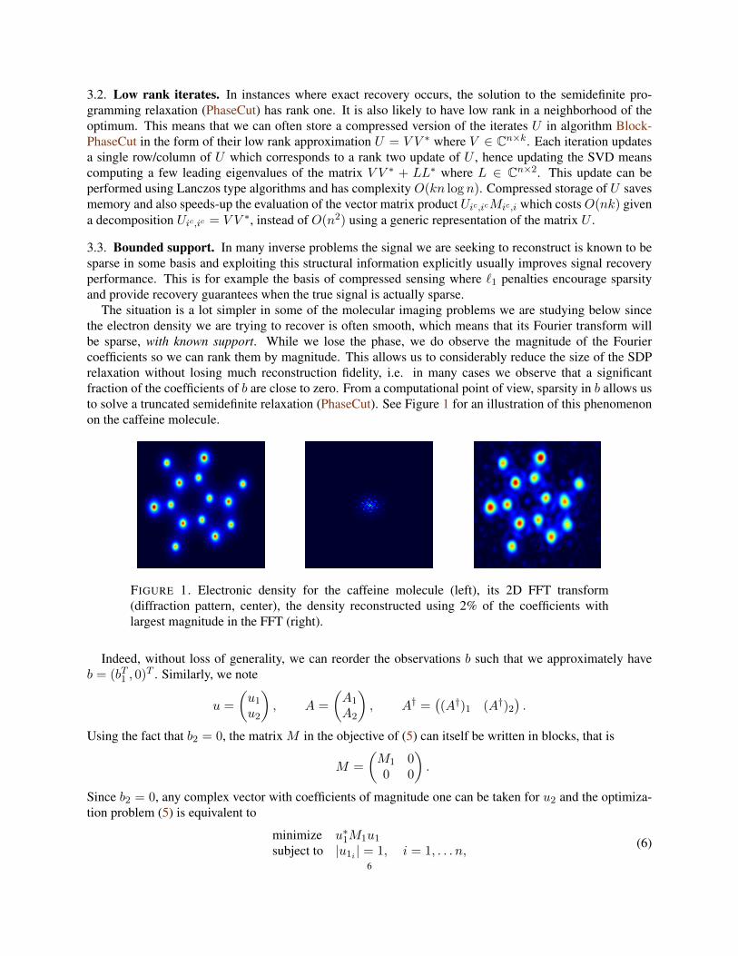
The situation is a lot simpler in some of the molecular imaging problems we are studying below sincethe electron density we are trying to recover is often smooth, which means that its Fourier transform willbe sparse, with known support. While we lose the phase, we do observe the magnitude of the Fouriercoefficients so we can rank them by magnitude. This allows us to considerably reduce the size of the SDPrelaxation without losing much reconstruction fidelity, i.e. in many cases we observe that a significantfraction of the coefficients of b are close to zero. From a computational point of view, sparsity in b allows usto solve a truncated semidefinite relaxation (PhaseCut). See Figure 1 for an illustration of this phenomenonon the caffeine molecule.

FIGURE 1. Electronic density for the caffeine molecule (left), its 2D FFT transform(diffraction pattern, center), the density reconstructed using 2% of the coefficients withlargest magnitude in the FFT (right).

Indeed, without loss of generality, we can reorder the observations b such that we approximately haveb = (bT1 , 0)T . Similarly, we note

u =

(u1u2

), A =

(A1

A2

), A† =

((A†)1 (A†)2

).

Using the fact that b2 = 0, the matrix M in the objective of (5) can itself be written in blocks, that is

M =

(M1 00 0

).

Since b2 = 0, any complex vector with coefficients of magnitude one can be taken for u2 and the optimiza-tion problem (5) is equivalent to

minimize u∗1M1u1subject to |u1i | = 1, i = 1, . . . n,

(6)

6

in the variable u1 ∈ Cn1 , where the Hermitian matrix

M1 = diag(b1)(I−A1(A†)1)diag(b1)

is positive semidefinite. This problem can in turn be relaxed into a PhaseCut problem which is usuallyconsiderably smaller than the original (PhaseCut) problem since M1 is typically a fraction of the size of M .

3.4. Real, positive densities. In some cases, such as imaging experiments where a random binary mask isprojected on an object for example, we know that the linear observations are formed as the Fourier transformof a positive measure. This introduces additional restrictions on the structure of these observations, whichcan be written as convex constraints on the phase vector. We detail two different ways of accounting for thispositivity assumption.

3.4.1. Direct nonnegativity constraints on the density. In the case where the signal is real and nonnegative,[Waldspurger et al., 2012] show that problem (3) can modified to specifically account for the fact that thesignal is real, by writing it

minu∈Cn, |ui|=1,

x∈Rp

‖Ax− diag(b)u‖22,

using the operator T (·) defined as

T (Z) =

(Re(Z) − Im(Z)Im(Z) Re(Z)

)(7)

we can rewrite the phase problem on real valued signal as

minimize∥∥∥∥T (A)

(x0

)− diag

(bb

)(Re(u)Im(u)

)∥∥∥∥22

subject to u ∈ Cn, |ui| = 1x ∈ Rp.

The optimal solution of the inner minimization problem in x is given by x = A†2B2v, where

A2 =

(Re(A)Im(A)

), B2 = diag

(bb

), and v =

(Re(u)Im(u)

)hence the problem is finally rewritten

minimize ‖(A2A†2B2 −B2)v‖22

subject to v2i + v2n+i = 1, i = 1, . . . , n,

in the variable v ∈ R2n. This can be relaxed as above by the following problem

minimize Tr(VM2)subject to Vii + Vn+i,n+i = 1, i = 1, . . . , n,

V � 0,(PhaseCutR)

which is a semidefinite program in the variable V ∈ S2n, where

M2 = (A2A†2B2 −B2)

T (A2A†2B2 −B2) = BT

2 (I−A2A†2)B2.

Because x = A†2B2v for real instances, we can add a nonnegativity constraint to this relaxation, using

xxT = (A†2B2)uuT (A†2B2)

T

and the relaxation becomesminimize Tr(VM2)

subject to (A†2B2)V (A†2B2)T ≥ 0,

Vii + Vn+i,n+i = 1, i = 1, . . . , n,V � 0,

7

which is a semidefinite program in V ∈ S2n.

3.4.2. Bochner’s theorem and the Fourier transform of positive measures. Another way to include nonnega-tivity constraints on the signal, which preserves some of the problem structure, is to use Bochner’s theorem.Recall that a function f : Rs 7→ C is positive semidefinite if and only if the matrix B with coefficientsBij = f(xi − xj) is Hermitian positive semidefinite for any sequence xi ∈ Rs. Bochner’s theorem thencharacterizes Fourier transforms of positive measures.

Theorem 3.1. (Bochner) A function f : Rs 7→ C is positive semidefinite if and only if it is the Fouriertransform of a (finite) nonnegative Borel measure.

Proof. See [Berg et al., 1984] for example.

For simplicity, we first illustrate this in dimension one. Suppose that we observe the magnitude of theFourier transform of a discrete nonnegative signal x ∈ Rp so that

|Fx| = b

with b ∈ Rn. Our objective now is to reconstruct a phase vector u ∈ Cn such that |u| = 1 and

Fx = diag(b)u.

If we define the Toeplitz matrix

Bij(y) = y|i−j|+1, 1 ≤ j ≤ i ≤ p,so that

B(y) =

y1 y∗2 · · · y∗ny2 y1 y∗2 · · ·

y2 y1 y∗2...

.... . . . . . . . .

. . . y2 y1 y∗2yn . . . y2 y1

then when Fx = diag(b)u, Bochner’s theorem states that B(diag(b)u) � 0 iff x ≥ 0. The contraintB(diag(b)u) � 0 is a linear matrix inequality in u, hence is convex.

Suppose that we observe multiple illuminations and that the k masks I1, . . . , Ik ∈ Rp×p are also nonneg-ative (e.g. random coherent illuminations), we have

Ax =

F(I1 ◦ x)...

F(Ik ◦ x)

,

and the phase retrieval problem (5) for positive signals x is now written

minimize u∗Musubject to Bj(diag(b)u) � 0, j = 1, . . . , k

|ui| = 1, i = 1, . . . n,

where Bj(y) is the matrix B(y(j)), where y(j) ∈ Cp is the jth subvector of y (one for each of the k masks).We can then adapt the PhaseCut relaxation to incorporate the positivity requirement. In the one dimensionalcase, using again the classical lifting argument in [Shor, 1987; Lovasz and Schrijver, 1991], it becomes

min. Tr(UM)subject to diag(U) = 1, u1 = 1,

Bj(diag(b)u) � 0, j = 1, . . . , k(U uu∗ 1

)� 0

(PhaseCut+)

8

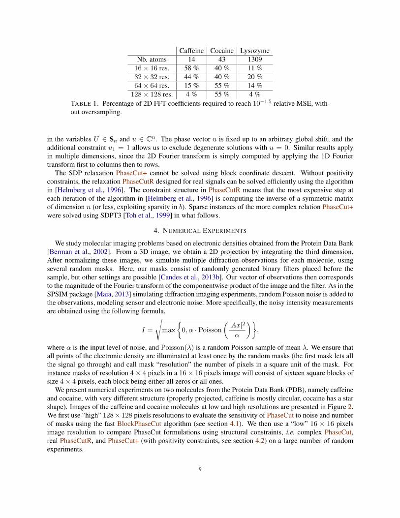
Caffeine Cocaine LysozymeNb. atoms 14 43 1309

16× 16 res. 58 % 40 % 11 %32× 32 res. 44 % 40 % 20 %64× 64 res. 15 % 55 % 14 %

128× 128 res. 4 % 55 % 4 %TABLE 1. Percentage of 2D FFT coefficients required to reach 10−1.5 relative MSE, with-out oversampling.

in the variables U ∈ Sn and u ∈ Cn. The phase vector u is fixed up to an arbitrary global shift, and theadditional constraint u1 = 1 allows us to exclude degenerate solutions with u = 0. Similar results applyin multiple dimensions, since the 2D Fourier transform is simply computed by applying the 1D Fouriertransform first to columns then to rows.

The SDP relaxation PhaseCut+ cannot be solved using block coordinate descent. Without positivityconstraints, the relaxation PhaseCutR designed for real signals can be solved efficiently using the algorithmin [Helmberg et al., 1996]. The constraint structure in PhaseCutR means that the most expensive step ateach iteration of the algorithm in [Helmberg et al., 1996] is computing the inverse of a symmetric matrixof dimension n (or less, exploiting sparsity in b). Sparse instances of the more complex relation PhaseCut+were solved using SDPT3 [Toh et al., 1999] in what follows.

4. NUMERICAL EXPERIMENTS

We study molecular imaging problems based on electronic densities obtained from the Protein Data Bank[Berman et al., 2002]. From a 3D image, we obtain a 2D projection by integrating the third dimension.After normalizing these images, we simulate multiple diffraction observations for each molecule, usingseveral random masks. Here, our masks consist of randomly generated binary filters placed before thesample, but other settings are possible [Candes et al., 2013b]. Our vector of observations then correspondsto the magnitude of the Fourier transform of the componentwise product of the image and the filter. As in theSPSIM package [Maia, 2013] simulating diffraction imaging experiments, random Poisson noise is added tothe observations, modeling sensor and electronic noise. More specifically, the noisy intensity measurementsare obtained using the following formula,

I =

√max

{0, α · Poisson

(|Ax|2α

)},

where α is the input level of noise, and Poisson(λ) is a random Poisson sample of mean λ. We ensure thatall points of the electronic density are illuminated at least once by the random masks (the first mask lets allthe signal go through) and call mask “resolution” the number of pixels in a square unit of the mask. Forinstance masks of resolution 4× 4 pixels in a 16× 16 pixels image will consist of sixteen square blocks ofsize 4× 4 pixels, each block being either all zeros or all ones.

We present numerical experiments on two molecules from the Protein Data Bank (PDB), namely caffeineand cocaine, with very different structure (properly projected, caffeine is mostly circular, cocaine has a starshape). Images of the caffeine and cocaine molecules at low and high resolutions are presented in Figure 2.We first use “high” 128× 128 pixels resolutions to evaluate the sensitivity of PhaseCut to noise and numberof masks using the fast BlockPhaseCut algorithm (see section 4.1). We then use a “low” 16 × 16 pixelsimage resolution to compare PhaseCut formulations using structural constraints, i.e. complex PhaseCut,real PhaseCutR, and PhaseCut+ (with positivity constraints, see section 4.2) on a large number of randomexperiments.

9

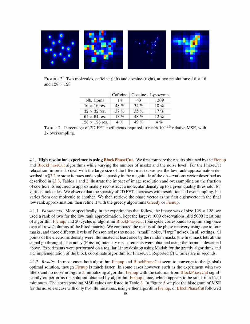
FIGURE 2. Two molecules, caffeine (left) and cocaine (right), at two resolutions: 16 × 16and 128× 128.

Caffeine Cocaine LysozymeNb. atoms 14 43 1309

16× 16 res. 48 % 34 % 10 %32× 32 res. 37 % 35 % 17 %64× 64 res. 13 % 48 % 12 %

128× 128 res. 4 % 49 % 4 %TABLE 2. Percentage of 2D FFT coefficients required to reach 10−1.5 relative MSE, with2x oversampling.

4.1. High resolution experiments using BlockPhaseCut. We first compare the results obtained by the Fienupand BlockPhaseCut algorithms while varying the number of masks and the noise level. For the PhaseCutrelaxation, in order to deal with the large size of the lifted matrix, we use the low rank approximation de-scribed in §3.2 to store iterates and exploit sparsity in the magnitude of the observations vector described asdescribed in §3.3. Tables 1 and 2 illustrate the impact of image resolution and oversampling on the fractionof coefficients required to approximately reconstruct a molecular density up to a given quality threshold, forvarious molecules. We observe that the sparsity of 2D FFTs increases with resolution and oversampling, butvaries from one molecule to another. We then retrieve the phase vector as the first eigenvector in the finallow rank approximation, then refine it with the greedy algorithms Greedy or Fienup.

4.1.1. Parameters. More specifically, in the experiments that follow, the image was of size 128 × 128, weused a rank of two for the low rank approximation, kept the largest 1000 observations, did 5000 iterationsof algorithm Fienup, and 20 cycles of algorithm BlockPhaseCut (one cycle corresponds to optimizing onceover all rows/columns of the lifted matrix). We compared the results of the phase recovery using one to fourmasks, and three different levels of Poisson noise (no noise, “small” noise, “large” noise). In all settings, allpoints of the electronic density were illuminated at least once by the random masks (the first mask lets all thesignal go through). The noisy (Poisson) intensity measurements were obtained using the formula describedabove. Experiments were performed on a regular Linux desktop using Matlab for the greedy algorithms anda C implementation of the block coordinate algorithm for PhaseCut. Reported CPU times are in seconds.

4.1.2. Results. In most cases both algorithm Fienup and BlockPhaseCut seem to converge to the (global)optimal solution, though Fienup is much faster. In some cases however, such as the experiment with twofilters and no noise in Figure 3, initializing algorithm Fienup with the solution from BlockPhaseCut signif-icantly outperforms the solution obtained by algorithm Fienup alone, which appears to be stuck in a localminimum. The corresponding MSE values are listed in Table 3. In Figure 5 we plot the histogram of MSEfor the noiseless case with only two illuminations, using either algorithm Fienup, or BlockPhaseCut followed

10

by greedy refinements, over many random illumination configurations. We observe that in many samples,algorithm Fienup gets stuck in a local optimum, while the SDP always converges to a global optimum.

1 ill., α = 0 2 ill., α = 0 3 ill., α = 0 4 ill., α = 0

1 ill., α = 10−3 2 ill., α = 10

−3 3 ill., α = 10−3 4 ill., α = 10

−3

1 ill., α = 10−2 2 ill., α = 10

−2 3 ill., α = 10−2 4 ill., α = 10

−2

FIGURE 3. Solution of the semidefinite relaxation algorithm BlockPhaseCut followed bygreedy refinements, for various values of the number of filters and noise level α.

Nb masks α SDP obj SDP Refined obj Fienup obj SDP time Fienup time1 0 0.410 0.021 0.046 104 782 0 2.157 0.069 0.877 179 1563 0 4.036 0.000 0.000 256 2414 0 7.075 0.000 0.000 343 3431 10−3 0.806 0.691 0.704 102 672 10−3 3.300 2.986 2.992 182 1443 10−3 5.691 5.276 5.277 263 2294 10−3 8.074 7.259 7.259 351 3081 10−2 3.299 3.187 3.193 104 712 10−2 7.492 8.622 8.646 182 1453 10−2 10.419 14.277 14.288 263 2224 10−2 14.139 21.472 21.444 349 305

TABLE 3. Performance comparison between algorithms Fienup and BlockPhaseCut forvarious values of the number of filters and noise level α. CPU times are in seconds.

11

1 ill., α = 0 2 ill., α = 0 3 ill., α = 0 4 ill., α = 0

1 ill., α = 10−3 2 ill., α = 10

−3 3 ill., α = 10−3 4 ill., α = 10

−3

1 ill., α = 10−2 2 ill., α = 10

−2 3 ill., α = 10−2 4 ill., α = 10

−2

FIGURE 4. Solution of the greedy algorithm Fienup, for various values of the number offilters and noise level α.

0.1 0.2 0.3 0.4 0.5 0.6 0.7 0.8 0.90

10

20

30

40

50

60

70

80

90

100

MSE

FIGURE 5. Histogram of MSE for the noiseless case with only two illuminations, usingeither algorithm Fienup (red), or BlockPhaseCut (blue) followed by greedy refinements,over many random starts.

4.2. Performance of PhaseCut relaxations with respect to number of masks, noise and filter resolution.We now compare PhaseCut formulations with structural constraints, i.e. complex PhaseCut, real PhaseCutR,and PhaseCut+ (with positivity constraints, see section 4.2) on a large number of random experimentsformed using “low” 16× 16 pixels image resolution.

12

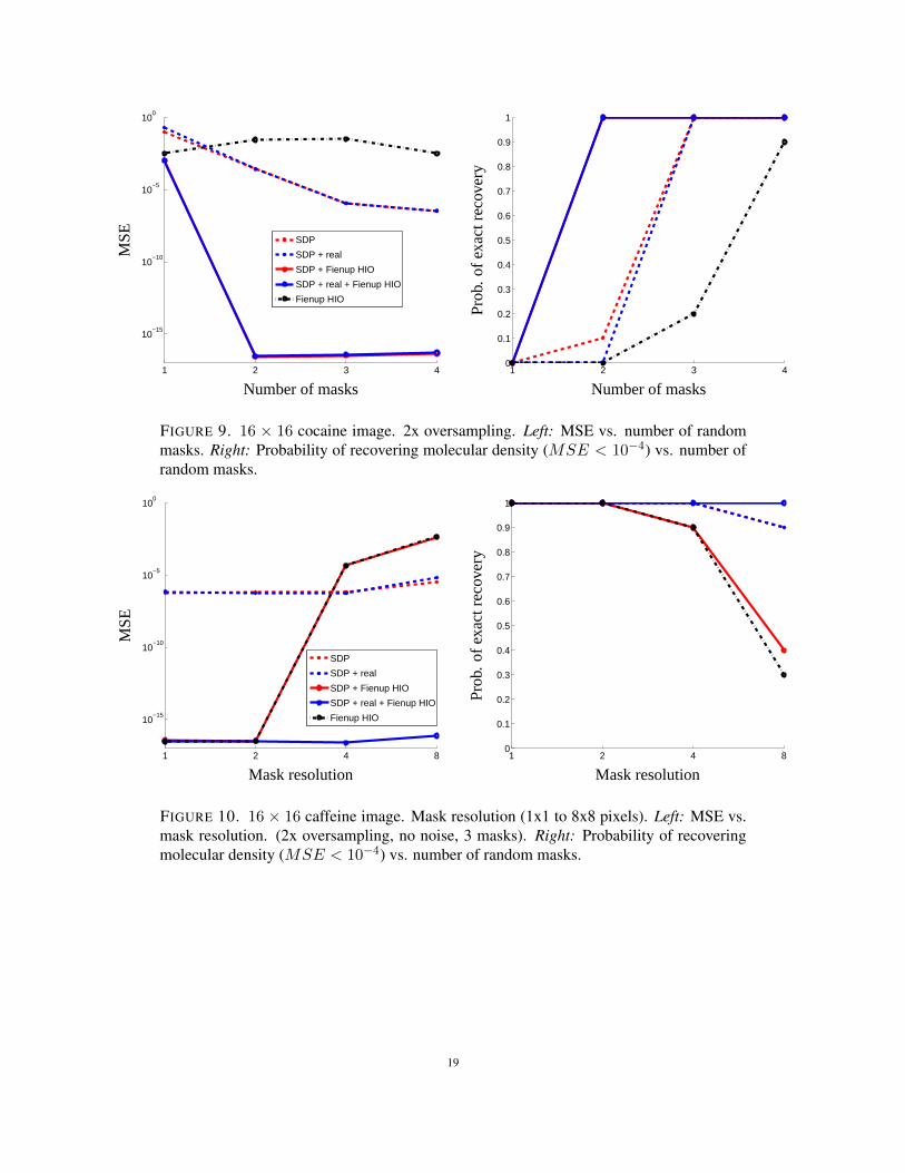
4.2.1. Varying the number of masks. Masks are of resolution 1 × 1 and no noise is added. As shown inFigures 6 and 7, PhaseCut, PhaseCutR and PhaseCut+ with Fienup post processing (respectively “SDP +Fienup HIO”, “SDP + real + Fienup HIO”, “SDP + real + toeplitz + Fienup HIO” and “Fienup HIO” curveson the figure) all outperform Fienup alone. For PhaseCut, in most cases, two to three masks seem enoughto exactly recover the phase. Moreover, as expected, PhaseCutR performs a little bit better than PhaseCut,but surprisingly, positivity constraints of PhaseCut+ do not seem to improve the solution of PhaseCutR inthese experiments. Finally, as shown in Figures 8 and 9, oversampling the Fourier transform seems to havea positive impact on the reconstruction. Results on caffeine and cocaine are very similar.

1 2 3 4 5 6

10−15

10−10

10−5

100

SDP

SDP + real

SDP + real + toeplitz

SDP + Fienup HIO

SDP + real + Fienup HIO

SDP + real + toeplitz + Fienup HIO

Fienup HIO

Number of masks

MSE

1 2 3 4 5 60

0.1

0.2

0.3

0.4

0.5

0.6

0.7

0.8

0.9

1

Number of masks

Prob

.of

exac

trec

over

y

FIGURE 6. 16 × 16 caffeine image. No oversampling. Left: MSE (relative to ‖b‖) vs.number of random masks. Right: Probability of recovering molecular density (MSE <10−4) vs. number of random masks.

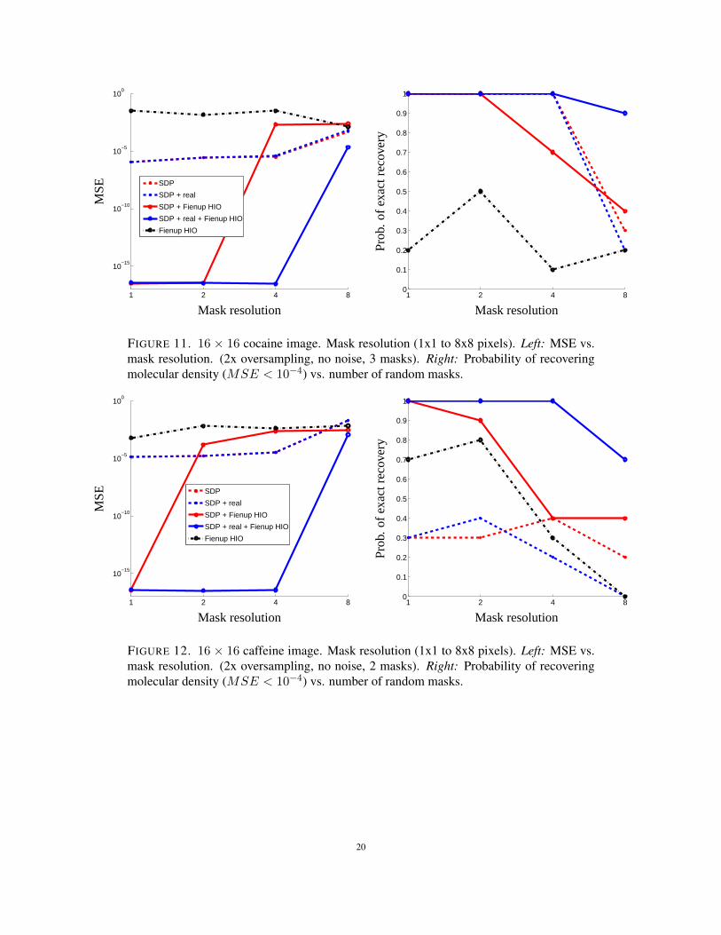
4.2.2. Varying mask resolution. Here, two or three masks are used and no noise is added. As shown inFigures 10, 11, 12 and 13, we can see that the MSE of reconstructed images increase with the resolution ofmasks. Moreover PhaseCutR is more robust to lower mask resolution than PhaseCut. Finally, as expected,with more randomly masked illuminations, we can afford to lower mask resolution.

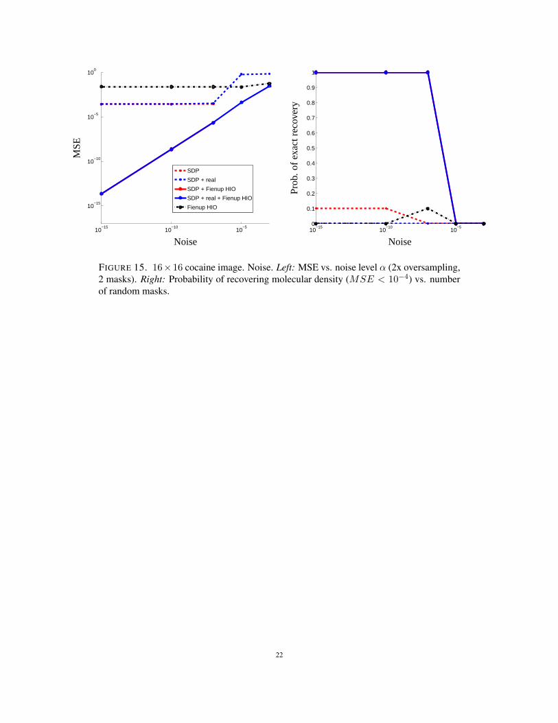
4.2.3. Varying noise levels. Here two masks are used (the minimum), with resolution 1× 1. Poisson noiseis added (parameterized by α). As shown in Figures 14, and 15, we can see that PhaseCut and PhaseCutRare stable with regards to noise, i.e. we obtain a linear increase of the log MSE with respect to the log noise.

5. USER GUIDE

We provide here the instructions to artificially recover the image of a molecule from the Protein DataBank using PhaseCutToolbox (download at www.di.ens.fr/˜aspremon). This example is entirelyreproduced with comments in the script testPhaseCut.m.

5.1. Installation. Our toolbox works on all recent versions of MATLAB on Mac OS X, and on MATLABversions anterior to 2008 on Linux (there might be conflicts with Arpack library for ulterior versions, whenusing BlockPhaseCut). Installation only requires to put the toolbox folder and subdirectories on the Matlabpath. Use for instance the command:>> addpath(genpath(’MYPATH/PhaseCutToolbox’));

where MYPATH is the directory where you have copied the toolbox.13

5.2. Generate the diffraction pattern of a molecule. Suppose we work with the caffeine molecule, on animage of resolution 128× 128 pixels. We set the corresponding input variables.>> nameMol=’caffeine.pdb’;>> N = 128 ;

Now, we set the parameters of the masks. The number of masks (also called filters or illuminations) is setto 2. Moreover we set the filter resolution to 1. The filter resolution corresponds to the square root of thenumber of pixels in each block of the binary filter. The filter resolution must divide N (the square root of thenumber of pixels in the image).>> filterRes = 1 ;>> nb_filters=2;

Since the filters are generated randomly, we set the seed of the uniform random generator to 1 in order toget reproducible experiments. Note that the quality of the phase retrieval may depend on the shape of thegenerated masks, especially when using only 2 or 3 filters.>> rand(’seed’,1);

Now we can generate an image, 2 masks and their corresponding diffraction patterns. We set the level ofnoise on the observations to zero here (i.e. no noise). α is the level of Poisson noise, and β is the level ofGaussian noise.>> alpha=0;>> beta=0;

We set the oversampling parameter for the Fourier transform to 2.>> OSF = 2;

The total number of observations, i.e. the size of the vector b is>> nbObs=N*N*OSF*OSF*nb_filters;

Suppose that we want to use only the first largest one thousand observations in PhaseCut, we set>> nbObsKept=1000;

Note that the number of observations that is sufficient to get close to the optimal solution depends on thesize of the data N and the sparsity of the vector b. From a more practical point of view, the larger nbObsKept,the more time intensive the optimization. Therefore, for a quick test we recommend setting nbObsKept to afew thousands, then increasing it if the results are not satisfying.

Finally we call the function genData which is going to generate both the image x we want to recover,filters, and observations b. bs corresponds to the thousand largest observations, xs is the image recoveredwith the true phase but using only bs. idx bs is the logical indicator vector of bs (bs=b(idx bs)). We putdisplayFig to 1 in order to display the filters, the images of the molecule x and xs, as well as the diffractionpatterns (with and without noise).>> displayFig=1;>> [x,b,filters,bs,xs,idx_bs] = genData(nameMol, nb_filters, ...filterRes, N, alpha, beta, OSF, nbObsKept, displayFig);

5.3. Phase Retrieval using Fienup and/or PhaseCut. Using the data generated in the previous section,we retrieve the phase of the observations vector b. Suppose we want to use the SDP relaxation with greedyrefinement, we set>> method=’SDPRefined’;

The other choices for method are ’Fienup’, ’Fienup HIO’ and ’SDP’ (no greedy refinement). We setthe initial (full) phase vector u to the vector of ones, and the number of iterations for Fienup algorithm to5000. The number of iterations for Fienup algorithm must be large enough so that the objective functionconverges to a stationary point. In most cases 5000 iterations seems to be enough.>> param.uInit=ones(nbObs,1);>> param.nbIterFienup=5000;

14

We also need to choose which algorithm we want to use in order to solve the SDP relaxation. For highresolution images, we recommend to always use the block coordinate descent algorithm with a low rankapproximation of the lifted matrix (BCDLR), since interior points methods (when using SDPT3 or Mosek)and block coordinate descent without low rank approximation (BCD) become very slow when the numberof observations used is over a few thousands.>> param.SDPsolver=’BCDLR’;

If we had wanted to solve PhaseCutR or PhaseCut+ we would have set>> param.SDPsolver=’realSDPT3’;

or>> param.SDPsolver=’ToepSDPT3’;

We can now set up the parameters for the BCDLR solver.>> param.nbCycles=20;>> param.r=2;

One cycle corresponds to optimizing over all the columns of the lifted matrix. In most cases, it seemsthat using nbCycles between 20 and 40 is enough to get close to the optimum, at least when refiningthe solution with Fienup algorithm. r is the rank for the low rank approximation of the lifted matrix.Similarly it seems that r between 2 and 4 gives reasonable results. Note that you can check that the lowrank approximation is valid by looking at the maximum ratio between the last and the first eigenvaluesthroughout all iterations of the BCDLR algorithm. This ratio is outputted as relax.eigRatio when callingthe function retrievePhase (see below). We finally call the function retrievePhase in order to solve theSDP relaxation with greedy refinement.>> data.b=b;>> data.bs=bs;>> data.idx_bs=idx_bs;>> data.OSF=OSF;>> data.filters=filters;>> [retrievedPhase, objValues, finalObj,relax] = retrievePhase(data,method,param);

The function retrievePhase outputs the vector of retrieved phase as retrievedPhase and the values of theobjective function at each iteration/cycle of the algorithm in objValues (add .Fienup, .SDP .SDPREfinedto retrievedPhase and objValues to get the corresponding retrieved phase and objective value). If usingthe SDP relaxation, the vector retrievedPhase is the first eigenvector of the final lifted matrix in PhaseCut.Note that the objective value in Fienup and in the SDP relaxation do not correspond exactly since thelifted matrix may be of rank bigger than one during the iterations of the BCDLR. Therefore we also outputfinalObj, which is the objective value of the phase vector extracted from the lifted matrix (i.e. the vectorretrievedPhase). The image can now be retrieved using the command>> xRetreived=pseudo_inverse_A(retrievedPhase.SDPRefined.*b,filters,M);

Finally you can visualize the results using the following standard Matlab commands, plotting the objectivevalues>> figure(1)>> subplot(2,1,1);>> title(method)>> plot(log10(abs(objValues))); axis tight

and displaying images>> subplot(2,3,4)>> imagesc(abs(x));axis off;>> subplot(2,3,5)>> imagesc(abs(xs));axis off;>> subplot(2,3,6)>> imagesc(abs(xRetreived)); axis off;

5.4. Reproduceing the experiments of the paper. All the numerical experiments of the paper can bereproduced using the Matlab scripts included in the toolbox directory Experiments.

• phaseTransition OSF1.m (evolution of MSE with number of filters, with no oversampling ofthe Fourier transform, Figures 6, 7)

15

• phaseTransition OSF2.m (evolution of MSE with number of filters, with oversampling of theFourier transform Figures 8, 9)• filterResTransition.m (evolution of MSE with filter resolution, figures 12, 13, 10, 11).• noiseTransition.m (evolution of MSE with noise, Figures 14, 15)• testNoiseNbIllums.m (test noise vs number of filters, Figures 3 and 4, and table 3)• testSeeds.m (test different seeds to generate filters, Figure 5)

ACKNOWLEDGMENTS

AA and FF would like to acknowledge support from a starting grant from the European Research Council(project SIPA).

REFERENCES

Heinz H Bauschke, Patrick L Combettes, and D Russell Luke. Phase retrieval, error reduction algorithm, and fienupvariants: a view from convex optimization. JOSA A, 19(7):1334–1345, 2002.

Stephen R Becker, Emmanuel J Candes, and Michael C Grant. Templates for convex cone problems with applicationsto sparse signal recovery. Mathematical Programming Computation, 3(3):165–218, 2011.

Christian Berg, Jens Peter Reus Christensen, and Paul Ressel. Harmonic analysis on semigroups : theory of positivedefinite and related functions, volume 100 of Graduate texts in mathematics. Springer-Verlag, New York, 1984.

H.M. Berman, T. Battistuz, TN Bhat, W.F. Bluhm, P.E. Bourne, K. Burkhardt, Z. Feng, G.L. Gilliland, L. Iype, S. Jain,et al. The protein data bank. Acta Crystallographica Section D: Biological Crystallography, 58(6):899–907, 2002.

O. Bunk, A. Diaz, F. Pfeiffer, C. David, B. Schmitt, D.K. Satapathy, and JF Veen. Diffractive imaging for periodicsamples: retrieving one-dimensional concentration profiles across microfluidic channels. Acta CrystallographicaSection A: Foundations of Crystallography, 63(4):306–314, 2007.

E. J. Candes, T. Strohmer, and V. Voroninski. Phaselift : exact and stable signal recovery from magnitude mea-surements via convex programming. To appear in Communications in Pure and Applied Mathematics, 66(8):1241–1274, 2013a.

E.J. Candes, Y. Eldar, T. Strohmer, and V. Voroninski. Phase retrieval via matrix completion. Arxiv preprintarXiv:1109.0573, 2011.

Emmanuel J Candes, Xiaodong Li, and Mahdi Soltanolkotabi. Phase retrieval from coded diffraction patterns. preprint,2013b.

A. Chai, M. Moscoso, and G. Papanicolaou. Array imaging using intensity-only measurements. Inverse Problems,27:015005, 2011.

Martin Dierolf, Andreas Menzel, Pierre Thibault, Philipp Schneider, Cameron M Kewish, Roger Wepf, Oliver Bunk,and Franz Pfeiffer. Ptychographic x-ray computed tomography at the nanoscale. Nature, 467(7314):436–439, 2010.

J.R. Fienup. Phase retrieval algorithms: a comparison. Applied Optics, 21(15):2758–2769, 1982.

R. Gerchberg and W. Saxton. A practical algorithm for the determination of phase from image and diffraction planepictures. Optik, 35:237–246, 1972.

Joseph Goodman. Introduction to fourier optics. 2008.

D. Griffin and J. Lim. Signal estimation from modified short-time fourier transform. Acoustics, Speech and SignalProcessing, IEEE Transactions on, 32(2):236–243, 1984.

R.W. Harrison. Phase problem in crystallography. JOSA A, 10(5):1046–1055, 1993.

C. Helmberg, F. Rendl, R. J. Vanderbei, and H. Wolkowicz. An interior–point method for semidefinite programming.SIAM Journal on Optimization, 6:342–361, 1996.

I Johnson, K Jefimovs, O Bunk, C David, M Dierolf, J Gray, D Renker, and F Pfeiffer. Coherent diffractive imagingusing phase front modifications. Physical review letters, 100(15):155503, 2008.

16

L. Lovasz and A. Schrijver. Cones of matrices and set-functions and 0-1 optimization. SIAM Journal on Optimization,1(2):166–190, 1991.

Filipe Maia. Spsim. 2013.

J. Miao, T. Ishikawa, Q. Shen, and T. Earnest. Extending x-ray crystallography to allow the imaging of noncrystallinematerials, cells, and single protein complexes. Annu. Rev. Phys. Chem., 59:387–410, 2008.

N.Z. Shor. Quadratic optimization problems. Soviet Journal of Computer and Systems Sciences, 25:1–11, 1987.

K. C. Toh, M. J. Todd, and R. H. Tutuncu. SDPT3 – a MATLAB software package for semidefinite programming.Optimization Methods and Software, 11:545–581, 1999.

I. Waldspurger, A. d’Aspremont, and S. Mallat. Phase recovery, maxcut and complex semidefinite programming.ArXiv: 1206.0102, 2012.

C.M.A.P., ECOLE POLYTECHNIQUE, UMR CNRS 7641E-mail address: fajwel.fogel@cmap.polytechnique.fr

D.I., ECOLE NORMALE SUPERIEURE, PARIS.E-mail address: waldspur@clipper.ens.fr

CNRS & D.I., UMR 8548,ECOLE NORMALE SUPERIEURE, PARIS, FRANCE.E-mail address: aspremon@ens.fr

17

1 2 3 4 5 6

10−15

10−10

10−5

100

SDP

SDP + real

SDP + real + toeplitz

SDP + Fienup HIO

SDP + real + Fienup HIO

SDP + real + toeplitz + Fienup HIO

Fienup HIO

Number of masks

MSE

1 2 3 4 5 60

0.1

0.2

0.3

0.4

0.5

0.6

0.7

0.8

0.9

1

Number of masks

Prob

.of

exac

trec

over

y

FIGURE 7. 16 × 16 cocaine image. No oversampling. Left: MSE (relative to ‖b‖) vs.number of random masks. Right: Probability of recovering molecular density (MSE <10−4) vs. number of random masks.

1 2 3 4

10−15

10−10

10−5

100

SDPSDP + realSDP + Fienup HIOSDP + real + Fienup HIOFienup HIO

Number of masks

MSE

1 2 3 40

0.1

0.2

0.3

0.4

0.5

0.6

0.7

0.8

0.9

1

Number of masks

Prob

.of

exac

trec

over

y

FIGURE 8. 16 × 16 caffeine image. 2x oversampling. Left: MSE vs. number of randommasks. Right: Probability of recovering molecular density (MSE < 10−4) vs. number ofrandom masks.

18

1 2 3 4

10−15

10−10

10−5

100

SDP

SDP + real

SDP + Fienup HIO

SDP + real + Fienup HIO

Fienup HIO

Number of masks

MSE

1 2 3 40

0.1

0.2

0.3

0.4

0.5

0.6

0.7

0.8

0.9

1

Number of masks

Prob

.of

exac

trec

over

y

FIGURE 9. 16 × 16 cocaine image. 2x oversampling. Left: MSE vs. number of randommasks. Right: Probability of recovering molecular density (MSE < 10−4) vs. number ofrandom masks.

1 2 4 8

10−15

10−10

10−5

100

SDP

SDP + real

SDP + Fienup HIO

SDP + real + Fienup HIO

Fienup HIO

Mask resolution

MSE

1 2 4 80

0.1

0.2

0.3

0.4

0.5

0.6

0.7

0.8

0.9

1

Mask resolution

Prob

.of

exac

trec

over

y

FIGURE 10. 16 × 16 caffeine image. Mask resolution (1x1 to 8x8 pixels). Left: MSE vs.mask resolution. (2x oversampling, no noise, 3 masks). Right: Probability of recoveringmolecular density (MSE < 10−4) vs. number of random masks.

19

1 2 4 8

10−15

10−10

10−5

100

SDP

SDP + real

SDP + Fienup HIO

SDP + real + Fienup HIO

Fienup HIO

Mask resolution

MSE

1 2 4 80

0.1

0.2

0.3

0.4

0.5

0.6

0.7

0.8

0.9

1

Mask resolution

Prob

.of

exac

trec

over

y

FIGURE 11. 16 × 16 cocaine image. Mask resolution (1x1 to 8x8 pixels). Left: MSE vs.mask resolution. (2x oversampling, no noise, 3 masks). Right: Probability of recoveringmolecular density (MSE < 10−4) vs. number of random masks.

1 2 4 8

10−15

10−10

10−5

100

SDP

SDP + real

SDP + Fienup HIO

SDP + real + Fienup HIO

Fienup HIO

Mask resolution

MSE

1 2 4 80

0.1

0.2

0.3

0.4

0.5

0.6

0.7

0.8

0.9

1

Mask resolution

Prob

.of

exac

trec

over

y

FIGURE 12. 16 × 16 caffeine image. Mask resolution (1x1 to 8x8 pixels). Left: MSE vs.mask resolution. (2x oversampling, no noise, 2 masks). Right: Probability of recoveringmolecular density (MSE < 10−4) vs. number of random masks.

20

1 2 4 8

10−15

10−10

10−5

100

SDP

SDP + real

SDP + Fienup HIO

SDP + real + Fienup HIO

Fienup HIO

Mask resolution

MSE

1 2 4 80

0.1

0.2

0.3

0.4

0.5

0.6

0.7

0.8

0.9

1

Mask resolution

Prob

.of

exac

trec

over

y

FIGURE 13. 16 × 16 cocaine image. Mask resolution (1x1 to 8x8 pixels). Left: MSE vs.mask resolution. (2x oversampling, no noise, 2 masks). Right: Probability of recoveringmolecular density (MSE < 10−4) vs. number of random masks.

10−15

10−10

10−5

10−15

10−10

10−5

100

SDP

SDP + real

SDP + Fienup HIO

SDP + real + Fienup HIO

Fienup HIO

Noise

MSE

10−15

10−10

10−5

0

0.1

0.2

0.3

0.4

0.5

0.6

0.7

0.8

0.9

1

Noise

Prob

.of

exac

trec

over

y

FIGURE 14. 16×16 caffeine image. Noise. Left: MSE vs. noise level α (2x oversampling,2 masks). Right: Probability of recovering molecular density (MSE < 10−4) vs. numberof random masks.

21

10−15

10−10

10−5

10−15

10−10

10−5

100

SDP

SDP + real

SDP + Fienup HIO

SDP + real + Fienup HIO

Fienup HIO

Noise

MSE

10−15

10−10

10−5

0

0.1

0.2

0.3

0.4

0.5

0.6

0.7

0.8

0.9

1

Noise

Prob

.of

exac

trec

over

y

FIGURE 15. 16×16 cocaine image. Noise. Left: MSE vs. noise level α (2x oversampling,2 masks). Right: Probability of recovering molecular density (MSE < 10−4) vs. numberof random masks.

22