phase space feynman path integrals via piecewise ... · pdf filephase space feynman path...

Bull. Sci. math. 132 (2008) 313–357www.elsevier.com/locate/bulsci

Phase space Feynman path integrals via piecewisebicharacteristic paths and their semiclassical

approximations

Naoto Kumano-go a,∗,1,2, Daisuke Fujiwara b,3

a Mathematics, Kogakuin University, 1-24-2 Nishishinjuku, Shinjuku-ku, Tokyo 163-8677, Japanb Department of Mathematics, Gakushuin University, 1-5-1 Mejiro, Toshima-ku, Tokyo 171-8588, Japan

Received 8 June 2007

Available online 22 June 2007

Abstract

We give a fairly general class of functionals for which the phase space Feynman path integrals have amathematically rigorous meaning. More precisely, for any functional belonging to our class, the time slicingapproximation of the phase space path integral converges uniformly on compact subsets of the phase space.Our class of functionals is rich because it is closed under addition and multiplication. The interchange of theorder with the Riemann integrals, the interchange of the order with a limit and the perturbation expansionformula hold in the phase space path integrals. The use of piecewise bicharacteristic paths naturally leadsus to the semiclassical approximation on the phase space.© 2007 Elsevier Masson SAS. All rights reserved.

MSC: 81S40; 35S30; 81Q20; 58D30

Keywords: Path integrals; Fourier integral operators; Semiclassical approximation

* Corresponding author.E-mail addresses: [email protected] (N. Kumano-go), [email protected] (D. Fujiwara).

1 This work was supported by MEXT. KAKENHI 18740077.2 This work was supported in Portugal at GFMUL by POCTI/MAT/34924.3 This work was supported by JSPS. KAKENHI(C)17540170.

0007-4497/$ – see front matter © 2007 Elsevier Masson SAS. All rights reserved.doi:10.1016/j.bulsci.2007.06.003

314 N. Kumano-go, D. Fujiwara / Bull. Sci. math. 132 (2008) 313–357

1. Introduction

Let u(T ) be the solution for the Schrödinger equation such that(ih̄∂T − H

(T ,x,

h̄

i∂x

))u(T ) = 0, u(0) = v, (1.1)

where 0 < h̄ < 1 is the Planck parameter. We can write u(T ) as follows:

u(T ) =(

1

2πh̄

)d ∫Rd

∫Rd

K(T , x, ξ0, x0)v(x0) dx0 dξ0. (1.2)

Using the phase space path integral which R.P. Feynman introduced in [7, Appendix B], we canformally write

K(T ,x, ξ0, x0) =∫

eih̄φ[q,p]D[q,p]. (1.3)

Here (q,p) : [0, T ] → R2d is the path in the phase space with q(T ) = x, q(0) = x0 and p(0) =ξ0, and φ[q,p] is the action along the path (q,p) defined by

φ[q,p] =∫

[0,T )

p(t) · dq(t) −∫

[0,T )

H(t, q(t),p(t)

)dt, (1.4)

and the phase space path integral∫ ∼ D[q,p] is a sum over all the paths (q,p). In [6], Feynman

explained his original configuration space path integral as a limit of a finite dimensional inte-gral, which is now called the time slicing approximation. Furthermore, Feynman considered theconfiguration space path integrals with general functional as integrand (cf. L.S. Schulman [28,Chapter 8], J.C. Zambrini [4, Part 2.4]). However, R.H. Cameron [3] proved that the measurefor the path integral does not exist in the sense of mathematics. Furthermore, in some papersof physics, the phase space path integral has some interpretations of the paths (q,p) (cf. [28,Chapter 31]).

In this paper, using the time slicing approximation via piecewise bicharacteristic paths, wetreat mathematically rigorously the phase space path integrals∫

eih̄φ[q,p]

F [q,p]D[q,p], (1.5)

for a general class F of functionals F [q,p]. More precisely, for any F [q,p] ∈ F , the timeslicing approximation of (1.5) converges uniformly on compact subsets of R3d with respect tothe endpoints (x, ξ0, x0), i.e., (1.5) is well-defined.

The class F is an algebra, i.e.,

F [q,p],G[q,p] ∈F �⇒ F [q,p] + G[q,p],F [q,p]G[q,p] ∈F (1.6)

and it contains the following examples of functionals F [q,p]:

(1) The evaluation functionals with respect to (t, q) independent of the momentum p,

F [q] = B(t, q(t)

), 0 � t � T (1.7)

of functions B such that |∂αx B(t, x)| � Cα(1+|x|)m for some m > 0. In particular, F [q,p] ≡

1 ∈ F , i.e., (1.3) is well-defined.

N. Kumano-go, D. Fujiwara / Bull. Sci. math. 132 (2008) 313–357 315

(2) The Riemann integrals

F [q,p] =∫

[T ′,T ′′]B

(t, q(t),p(t)

)dt (1.8)

of functions B so that |∂αx ∂

βξ B(t, x, ξ)| � Cα,β(1 + |x| + |ξ |)m for some m > 0.

(3) The analytic functions of the integral

F [q] = f

( ∫[T ′,T ′′]

B(t, q(t)

)dt

)(1.9)

if B satisfies |∂αx B(t, x)| � Cα .

As an application, we can interchange the order of the phase space path integration and theRiemann integration, i.e.,∫

eih̄φ[q,p]

( ∫[T ′,T ′′]

B(t, q(t)

)dt

)D[q,p]

=∫

[T ′,T ′′]

(∫e

ih̄φ[q,p]

B(t, q(t)

)D[q,p]

)dt. (1.10)

We can also interchange the order of the limits and the phase space path integration: If fk , f areanalytic and limk→∞ ‖fk − f ‖μ,A = 0, then

limk→∞

∫e

ih̄φ[q,p]

fk

( ∫[T ′,T ′′]

B(t, q(t)

)dt

)D[q,p]

=∫

eih̄φ[q,p]

f

( ∫[T ′,T ′′]

B(t, q(t)

)dt

)D[q,p]. (1.11)

These two imply the perturbation expansion formula. Furthermore, the use of piecewise bichar-acteristic paths naturally leads us to the semiclassical approximation on the phase space, i.e.,∫

eih̄φ[q,p]

F [q,p]D[q,p]

= eih̄φ[qT,0,pT,0](D(T ,x, ξ0)

−1/2F [qT,0,pT,0] + O(h̄)), (1.12)

where qT,0 = qT,0(t, x, ξ0, x0), pT,0 = pT,0(t, x, ξ0) is the bicharacteristic path defined by (2.9)

and D(T ,x, ξ0) is a Hamiltonian version of the Morette-Van Vleck determinant [26].

Remark 1.1. Using Fourier integral operators, H. Kitada–H. Kumano-go [20] proved the uniformconvergence on R3d of the time slicing approximation of the phase space path integral (1.3), i.e.,the case of (1.5) with F [q,p] ≡ 1 (cf. N. Kumano-go [22]). In this sense, this paper has its originin [20].

Remark 1.2. D. Fujiwara [8] proved that the time slicing approximation of the configurationspace path integral converges uniformly on the configuration space. Furthermore, the author andD. Fujiwara [11,13,25] treated the configuration space path integrals with general functional asintegrand.


Remark 1.3. Although the present paper deals with the phase space path integrals, its discus-sion follows the discussion of N. Kumano-go [25] which treated the configuration space pathintegrals.

Remark 1.4. Using broken line paths of position and piecewise constant paths of momen-tum, W. Ichinose [16] discussed (1.5) in the case when F [q,p] = ∏K

k=1 zk(q(τk),p(τk)),0 < τ1 < τ2 < · · · < τK < T as an operator and gave some examples for which the time slic-ing approximations of (1.5) diverge as an operator. Note that (1.7) excludes the functionals ofthe type F [q,p] = B(t, q(t),p(t)).

Remark 1.5. The phase space path integrals via Fourier integral operators or pseudo-differentialoperators are also used in other equations (cf. J. Le Rousseau [18], N. Kumano-go [23], etc.).

Many people have given mathematically rigorous meanings to Feynman path integrals. E. Nel-son [27] formulated the configuration space path integral via the Trotter formula and connectedthe configuration space path integral to Wiener measure via analytic continuation. K. Itô [17]and S. Albeverio–Høegh Krohn [1] defined the configuration space path integrals via Fresnelintegral transform. I. Daubechies–J.R. Klauder [5] presented the phase space path integral via an-alytic continuation of the phase space Wiener measure. S. Albeverio–G. Guatteri–S. Mazzucchi[2] formulated the phase space path integral via Fresnel integral transform. O.G. Smolyanov–A.G. Tokarev–A. Truman [30] formulated the phase space path integral via the Chernoff formula.G.W. Johnson–M. Lapidus [19] and T.L. Gill–W.W. Zachary [15] developed Feynman’s opera-tional calculus of the main part of [7].

2. Main results

Our assumption for the Hamiltonian function H(t, x, ξ) of (1.1) is the following:

Assumption 1. H(t, x, ξ) is a real-valued function of (t, x, ξ) ∈ R×Rd ×Rd , and for any multi-indices α, β , ∂α

x ∂βξ H(t, x, ξ) is continuous in R×Rd ×Rd . For any non-negative integer k, there

exists a positive constant κk such that∣∣∂αx ∂

βξ H(t, x, ξ)

∣∣ � κk

(1 + |x| + |ξ |)max(2−|α+β|,0)

, (2.1)

for any multi-indices α, β with |α + β| = k.

Remark 2.1. The following Hamiltonian H(t, x, h̄i∂x) satisfies Assumption 1.

H

(t, x,

h̄

i∂x

)=

d∑j,k=1

(aj,k(t)

h̄

i∂xj

h̄

i∂xk

+ bj,k(t)xj

h̄

i∂xk

+ cj,k(t)xj xk

)

+d∑

j=1

(aj (t)

h̄

i∂xj

+ bj (t)xj

)+ c(t, x). (2.2)

Here aj,k(t), bj,k(t), cj,k(t), aj (t), bj (t) and ∂αx c(t, x) with any multi-index α are real-valued

continuous bounded functions.


Let ΔT,0 = (TJ+1, TJ , . . . , T1, T0) be an arbitrary division of the interval [0, T ] into subinter-vals, i.e.,

ΔT,0: T = TJ+1 > TJ > · · · > T1 > T0 = 0. (2.3)

Set tj = Tj −Tj−1 for j = 1,2, . . . , J, J +1. Let |ΔT,0| be the mesh of the division ΔT,0 definedby |ΔT,0| = max1�j�J+1 tj . Set xJ+1 = x. Let xj ∈ Rd and ξj ∈ Rd for j = 1,2, . . . , J .

Lemma 2.1. Let j = 1,2, . . . , J, J + 1 and κ2d(Tj − Tj−1) < 1/2. Then, for any (xj , ξj−1) ∈Rd × Rd , there exists a unique solution

q̄Tj ,Tj−1(t) = q̄Tj ,Tj−1(t, xj , ξj−1), p̄Tj ,Tj−1(t) = p̄Tj ,Tj−1(t, xj , ξj−1), (2.4)

of the system of equations

∂t q̄Tj ,Tj−1(t) = (∂ξH)(t, q̄Tj ,Tj−1(t), p̄Tj ,Tj−1(t)

), Tj−1 � t � Tj ,

∂t p̄Tj ,Tj−1(t) = −(∂xH)(t, q̄Tj ,Tj−1(t), p̄Tj ,Tj−1(t)

), Tj−1 � t � Tj ,

q̄Tj ,Tj−1(Tj ) = xj , p̄Tj ,Tj−1(Tj−1) = ξj−1. (2.5)

Using q̄Tj ,Tj−1(t) and p̄Tj ,Tj−1(t), we define the piecewise bicharacteristic path

qΔT,0(t) = qΔT,0(t, xJ+1, ξJ , xJ , ξJ−1, . . . , x1, ξ0, x0),

pΔT,0(t) = pΔT,0(t, xJ+1, ξJ , xJ , ξJ−1, . . . , x1, ξ0), (2.6)

by

qΔT,0(t) = q̄Tj ,Tj−1(t, xj , ξj−1), Tj−1 < t � Tj , qΔT,0(0) = x0,

pΔT,0(t) = p̄Tj ,Tj−1(t, xj , ξj−1), Tj−1 � t < Tj , (2.7)

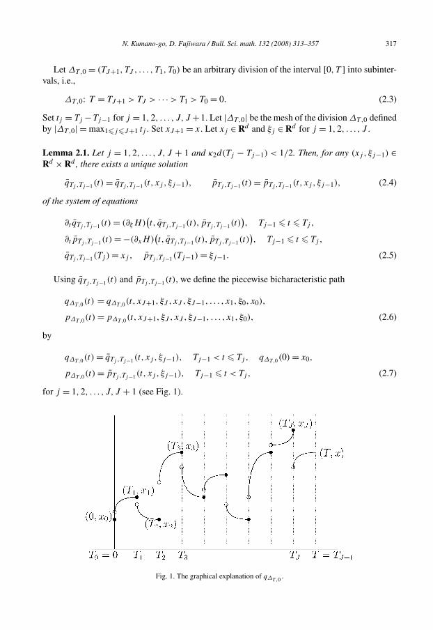
for j = 1,2, . . . , J, J + 1 (see Fig. 1).

Fig. 1. The graphical explanation of qΔT,0 .


Remark 2.2. Note that qΔT,0(t) is left-continuous and pΔT,0(t) is right-continuous on [0, T ), i.e.,

limt↑Tj

qΔT,0(t) = xj = qΔT,0(Tj ), limt↓Tj−1

pΔT,0(t) = ξj−1 = pΔT,0(Tj−1),

limt↓Tj−1

qΔT,0(t) = q̄Tj ,Tj−1(Tj−1), xj−1 = qΔT,0(Tj−1),

limt↑Tj

pΔT,0(t) = p̄Tj ,Tj−1(Tj ), ξj = pΔT,0(Tj ). (2.8)

(Our discussion about jumps at t = Tj , j = 0,1,2, . . . , J , was inspired by Zambrini [4, Part 2.4]and Schulman [28, Chapter 31].)

Remark 2.3. Note that qT,0(t) = qT,0(t, x, ξ0, x0), pT,0(t) = pT,0(t, x, ξ0) of Theorem 3 satisfy

qT,0(t) = q̄T ,0(t, x, ξ0), 0 < t � T , qT,0(0) = x0,

pT,0(t) = p̄T ,0(t, x, ξ0), 0 � t < T . (2.9)

We define the phase space Feynman path integral (1.5) by∫e

ih̄φ[q,p]

F [q,p]D[q,p]

= lim|ΔT,0|→0

(1

2πh̄

)dJ ∫R2dJ

eih̄φ[qΔT,0 ,pΔT,0 ]

F [qΔT,0 ,pΔT,0 ]J∏

j=1

dξj dxj , (2.10)

if the limit of the right-hand side exists.

Remark 2.4. Though φ[qΔT,0 ,pΔT,0 ], F [qΔT,0 ,pΔT,0] are functions of xJ+1, ξJ , xJ , . . . , ξ0, x0,i.e.,

φ[qΔT,0 ,pΔT,0 ] = φΔT,0(xJ+1, ξJ , xJ , . . . , ξ1, x1, ξ0, x0),

F [qΔT,0 ,pΔT,0] = FΔT,0(xJ+1, ξJ , xJ , . . . , ξ1, x1, ξ0, x0), (2.11)

we use the notation φ[qΔT,0 ,pΔT,0], F [qΔT,0 ,pΔT,0] in (2.10).

Remark 2.5. Even when F [q,p] = 1, the integrals of the right-hand side of (2.10) do notconverge absolutely. We treat the multiple integral in (2.10) as an oscillatory integral (cf.H. Kumano-go [21]).

Definition 1 (The class F ). Let F [q,p] be a functional whose domain contains all the piecewisebicharacteristic paths qΔT,0(t), pΔT,0(t) of (2.6). We say that F [q,p] ∈ F if F [q,p] satisfiesAssumption 2.

Assumption 2. Let m be a non-negative integer. Let U be a non-negative constant and letuj , j = 1,2, . . . , J, J + 1 are non-negative parameters depending on the division ΔT,0 suchthat

∑J+1j=1 uj � U < ∞. For any non-negative integer M , there exist positive constants AM ,

XM such that for any division ΔT,0, any multi-indices αj , βj−1 with |αj |, |βj−1| � M ,j = 1,2, . . . , J, J + 1 and any integer k with 1 � k � J ,


∣∣∣∣∣(

J+1∏j=1

∂αjxj

∂βj−1ξj−1

)FΔT,0(xJ+1, ξJ , . . . , x1, ξ0, x0)

∣∣∣∣∣� AM(XM)J+1

(J+1∏j=1

(tj )min(|βj−1|,1)

)(1 +

J+1∑j=1

(|xj | + |ξj−1|) + |x0|

)m

, (2.12)

∣∣∣∣∣(

J+1∏j=1

∂αjxj

∂βj−1ξj−1

)∂xk

FΔT,0(xJ+1, ξJ , . . . , x1, ξ0, x0)

∣∣∣∣∣� AM(XM)J+1uk

( ∏j �=k

(tj )min(|βj−1|,1)

)(1 +

J+1∑j=1

(|xj | + |ξj−1|) + |x0|

)m

. (2.13)

Theorem 1 (Existence of path integrals). Let T be sufficiently small. Then, for any F [q,p] ∈F , the right-hand side of (2.10) converges on compact subsets of (x, ξ0, x0) ∈ Rd × Rd × Rd ,together with all its derivatives in x and ξ0.

Remark 2.6. The size of T depends only on d and κ2 of Assumption 1.

Theorem 2 (Algebra). If F [q,p] ∈ F and G[q,p] ∈ F , then F [q,p] + G[q,p] ∈ F andF [q,p]G[q,p] ∈ F .

Remark 2.7. Applying Theorem 2 to the examples of Theorems 4, 5, 6, the reader can producemany functionals F [q,p] ∈F .

Theorem 3 (Semiclassical approximation as h̄ → 0). Let T be sufficiently small. Then, for anyF [q,p] ∈ F , we can write∫

eih̄φ[q,p]

F [q,p]D[q,p]

= eih̄φ[qT,0,pT,0](D(T ,x, ξ0)

−1/2F [qT,0,pT,0] + h̄Υ (T , h̄, x, ξ0, x0)). (2.14)

Here qT,0 = qT,0(t, x, ξ0, x0), pT,0 = pT,0(t, x, ξ0) is the bicharacteristic path defined by (2.9)and D(T ,x, ξ0) is the function given by (3.6). Furthermore, for any non-negative integer M ,there exist a positive constant CM and a positive integer M ′ independent of 0 < h̄ < 1 such that∣∣∂α

x ∂βξ0

Υ (T , h̄, x, ξ0, x0)∣∣ � CMAM ′T (U + T )

(1 + |x| + |ξ0| + |x0|

)m, (2.15)

for any multi-indices α, β with |α|, |β| � M .

Remark 2.8. As a simple case of (2.11) when T = T1 > T0 = 0, we write

φ[qT,0,pT,0] = φT,0(x, ξ0, x0), F [qT,0,pT,0] = FT,0(x, ξ0, x0). (2.16)

As we will see in Lemma 5.2, ωT,0(x, ξ0) = φT,0(x, ξ0, x0)− (x − x0) · ξ0 satisfies the followingestimate:∣∣∂α

x ∂βξ0

ωT,0(x, ξ0)∣∣ � Cα,βT

(1 + |x| + |ξ0|

)max(2−|α+β|,0). (2.17)

As we saw in Assumption 2, FT,0(x, ξ0, x0) satisfies the following estimate:∣∣∂αx ∂

βξ0

FT,0(x, ξ0, x0)∣∣ � AMXM(t1)

min(|β0|,1)(1 + |x| + |ξ0| + |x0|

)m. (2.18)


Remark 2.9. For the semiclassical approximation of the configuration space path integrals via thetime slicing approximation, see D. Fujiwara–N. Kumano-go [10,13,25]. For the semiclassical ap-proximation of the configuration space path integrals via Fresnel transform, see J. Rezende [29].

Theorem 4. Let m be a non-negative integer. Let 0 � T ′ � T ′′ � T . Assume that for any multi-indices α, β , ∂α

x ∂βξ B(t, x, ξ) is continuous on [T ′, T ′′] × Rd × Rd and there exists a positive

constant Cα,β such that∣∣∂αx ∂

βξ B(t, x, ξ)

∣∣ � Cα,β

(1 + |x| + |ξ |)m

. (2.19)

Then its Riemann integral belongs to the class F , i.e.,

F [q,p] =∫

[T ′,T ′′]B

(t, q(t),p(t)

)dt ∈F . (2.20)

Theorem 5 (Interchange of the order with Riemann integrals). Let m be a non-negative integer.Let 0 � T ′ � T ′′ � T . Assume that for any multi-index α, ∂α

x B(t, x) is continuous on [T ′, T ′′] ×Rd and there exists a positive constant Cα such that∣∣∂α

x B(t, x)∣∣ � Cα

(1 + |x|)m

. (2.21)

Then we have the following:

(1) The value at a fixed time t , 0 � t � T ,

F [q] = B(t, q(t)

) ∈ F . (2.22)

(2) Let T be sufficiently small. Then, for any F [q,p] ∈ F including F [q,p] ≡ 1, we have∫e

ih̄φ[q,p]

( ∫[T ′,T ′′]

B(t, q(t)

)dt

)F [q,p]D[q,p]

=∫

[T ′,T ′′]

(∫e

ih̄φ[q,p]

B(t, q(t)

)F [q,p]D[q,p]

)dt. (2.23)

Theorem 6 (Interchange of the order with a limit). Let f (b) be an analytic function of b ∈ C ona neighborhood of zero, i.e., there exist positive constants μ > 0, A > 0 such that

‖f ‖μ,A ≡ supn,|b|�μ

|∂nb f (b)|Ann! < ∞. (2.24)

Assume that B(t, x) satisfies the assumption of Theorem 5 with m = 0. Then we have the follow-ing:

(1) F [q] = f

( ∫[T ′,T ′′]

B(t, q(t)

)dt

)∈F . (2.25)

(2) Let T be sufficiently small. Let fk(b), k = 1,2,3, . . . , be analytic functions such thatlimk→∞ ‖fk − f ‖μ,A = 0. Then, for any F [q,p] ∈F including F [q,p] ≡ 1, we have


limk→∞

∫e

ih̄φ[q,p]

fk

( ∫[T ′,T ′′]

B(t, q(t)

)dt

)F [q,p]D[q,p]

=∫

eih̄φ[q,p]

f

( ∫[T ′,T ′′]

B(t, q(t)

)dt

)F [q,p]D[q,p]. (2.26)

Corollary 1 (Perturbation expansion formula). Let T be sufficiently small. Let B(t, x) satisfy theassumption of Theorem 5 with m = 0. Then we have∫

eih̄φ[q,p]+ i

h̄

∫[T ′,T ′′] B(t,q) dtD[q,p]

=∞∑

n=0

(i

h̄

)n ∫[T ′,T ′′]

dτn

∫[T ′,τn]

dτn−1 · · ·∫

[T ′,τ2]dτ1

×∫

eih̄φ[q,p]

B(τn, q(τn)

)B

(τn−1, q(τn−1)

) · · ·B(τ1, q(τ1)

)D[q,p]. (2.27)

3. Results on convergence

For simplicity, for 1 � l � L � J , we write

xL,l = (xL, xL−1, . . . , xl+1, xl), ξL,l = (ξL, ξL−1, . . . , ξl+1, ξl). (3.1)

Lemma 3.1. Let 4κ2dT < 1/2. Then, for any (xJ+1, ξ0) ∈ Rd ×Rd , there exists a unique solutionx∗J,1 = x∗

J,1(xJ+1, ξ0), ξ∗J,1 = ξ∗

J,1(xJ+1, ξ0) of the system of equations

(∂(xJ,1,ξJ,1)φΔT,0)(xJ+1, ξ∗J , x∗

J , . . . , ξ∗1 , x∗

1 , ξ0) = 0. (3.2)

For any given function f = f (xJ+1, ξJ , xJ , . . . , ξ1, x1, ξ0, x0), let f ∗ be the function obtainedby putting xJ,1 = x∗

J,1, ξJ,1 = ξ∗J,1 into f , i.e.,

f ∗ = f ∗(xJ+1, ξ0, x0) = f (xJ+1, ξ∗J , x∗

J , . . . , ξ∗1 , x∗

1 , ξ0, x0). (3.3)

We define DΔT,0(xJ+1, ξ0) by

DΔT,0(xJ+1, ξ0) = (−1)dJ det(∂2(ξJ ,xJ ,...,ξ1,x1)

φΔT,0

)∗. (3.4)

Theorem 7. Let T be sufficiently small. For any multi-indices α, β , there exists a positive con-stant Cα,β independent of ΔT,0 such that

∣∣∂αx ∂

βξ0

(DΔT,0(x, ξ0) − 1)∣∣ � Cα,βT 2, (3.5)∣∣∂α

x ∂βξ0

(DΔT,0(x, ξ0) − D(T ,x, ξ0)

)∣∣ � Cα,β |ΔT,0|T , (3.6)

with a function D(T ,x, ξ0).

We define bΔ (h̄, xJ+1, ξ0, x0) by
T ,0


eih̄φ[qT,0,pT,0]bΔT,0(h̄, xJ+1, ξ0, x0)

=(

1

2πh̄

)dJ ∫R2dJ


F [qΔT,0 ,pΔT,0]J∏

j=1

dξj dxj . (3.7)

Furthermore, we define the remainder term ΥΔT,0(h̄, xJ+1, ξ0, x0) by

bΔT,0(h̄, xJ+1, ξ0, x0) = DΔT,0(xJ+1, ξ0)−1/2F [qT,0,pT,0]

+ h̄ΥΔT,0(h̄, xJ+1, ξ0, x0). (3.8)

Theorem 8. Let T be sufficiently small. Then, for any non-negative integer M , there exist apositive constant CM and a positive integer M ′ independent of 0 < h̄ < 1 such that for anydivision ΔT,0 and any multi-indices α, β with |α|, |β| � M ,∣∣∂α

x ∂βξ0

ΥΔT,0(h̄, x, ξ0, x0)∣∣

� CMAM ′T (T + U)(1 + |x| + |ξ0| + |x0|

)m, (3.9)∣∣∂α

x ∂βξ0

(ΥΔT,0(h̄, x, ξ0, x0) − Υ (T , h̄, x, ξ0, x0)

)∣∣� CMAM ′ |ΔT,0

∣∣(T + U)(1 + |x| + |ξ0| + |x0

∣∣)m, (3.10)

with a function Υ (T , h̄, x, ξ0, x0).

4. Proof of Theorems 1–6

From now on, our discussion is similar to the one in N. Kumano-go [25]. Assuming Theo-rems 7, 8, we prove Theorems 1–6 in this section. We will prove Theorems 7, 8 step by step inthe later sections.

Proof of Theorem 1. By (3.7) and (3.8), we can write (2.10) as∫e

ih̄φ[q,p]

F [q,p]D[q,p] = lim|ΔT,0|→0e

ih̄φ[qT,0,pT,0]

× (DΔT,0(x, ξ0)

−1/2F [qT,0,pT,0] + h̄ΥΔT,0(h̄, x, ξ0, x0)). (4.1)

By Theorems 7, 8, the right-hand side of (2.10) converges on any compact subset of R3d . �Proof of Theorem 2. This follows from Assumption 2. �Proof of Theorem 3. This follows from (4.1) and Theorems 7, 8. �Proof of Theorem 4. For simplicity, we set 0 = T ′ < T ′′ < T . Using l such that Tl−1 < T ′′ � Tl ,we can write

FΔT,0 =l−1∑j=1

∫[Tj−1,Tj ]

B(t, q̄Tj ,Tj−1(t), p̄Tj ,Tj−1(t)

)dt

+∫

′′B

(t, q̄Tl ,Tl−1(t), p̄Tl ,Tl−1(t)

)dt. (4.2)

[Tl−1,T ]


If j < l, we have

(∂ξj−1FΔT,0)(xj , ξj−1)

=∫

[Tj−1,Tj ](∂xB)

(t, q̄Tj ,Tj−1(t), p̄Tj ,Tj−1(t)

)(∂ξj−1 q̄Tj ,Tj−1(t)

)dt

+∫

[Tj−1,Tj ](∂ξB)


)(∂ξj−1 p̄Tj ,Tj−1(t)

)dt, (4.3)

(∂xjFΔT,0)(xj , ξj−1)

=∫

[Tj−1,Tj ](∂xB)


)(∂xj

q̄Tj ,Tj−1(t))dt

+∫

[Tj−1,Tj ](∂ξB)


)(∂xj

p̄Tj ,Tj−1(t))dt. (4.4)

By Lemma 5.1, for any multi-indices α, β , there exists a positive constant Cα,β such that∣∣∂αxj

∂βξj−1

(∂ξj−1FΔT,0)(xj , ξj−1)∣∣ � Cα,βtj

(1 + |xj | + |ξj−1|

)m, (4.5)∣∣∂α

xj∂

βξj−1

(∂xjFΔT,0)(xj , ξj−1)

∣∣ � Cα,βtj(1 + |xj | + |ξj−1|

)m. (4.6)

Set uj = tj for j < l, ul = (T ′′ − Tl−1) and uj = 0 for j > l. Then∑J+1

j=1 uj = T ′′ < ∞. HenceFΔT,0 satisfies Assumption 2. �Proof of Theorem 5. (1) Using l such that Tl−1 < t � Tl , we can write

FΔT,0(xl, ξl−1) = B(t, q̄Tl ,Tl−1(t)

), (4.7)

∂ξl−1FΔT,0(xl, ξl−1) = (∂xB)(t, q̄Tl ,Tl−1(t)

)(∂ξl−1 q̄Tl ,Tl−1(t)

), (4.8)

∂xlFΔT,0(xl, ξl−1) = (∂xB)

(t, q̄Tl ,Tl−1(t)

)(∂xl

q̄Tl ,Tl−1(t)). (4.9)

By Lemma 5.1, for any multi-indices α, β , there exists a positive constant Cα,β such that∣∣∂αxl

∂βξl−1

(∂ξl−1FΔT,0)(xl, ξl−1)∣∣ � Cα,β tl

(1 + |xl | + |ξl−1|

)m, (4.10)∣∣∂α

xl∂

βξl−1

(∂xlFΔT,0)(xl, ξl−1)

∣∣ � Cα,β

(1 + |xl | + |ξl−1|

)m. (4.11)

Set uj = 0 for j �= l and ul = 1. Then∑J+1

j=1 uj = 1 < ∞. Hence FΔT,0 satisfies Assumption 2.(2) For simplicity, we set F [q,p] ≡ 1 and 0 = T ′ < T ′′ = T .∫

eih̄φ[q,p]

∫[T ′,T ′′]

B(t, q(t)

)dt D[q,p]

= lim|ΔT,0|→0

(1

2πh̄

)dJ ∫R2dJ


∫[T ′,T ′′]

B(t, qΔT,0(t)

)dt

J∏j=1

dξj dxj

= lim|ΔT,0|→0

J+1∑l=1

(1

2πh̄

)dJ ∫2dJ


∫B

(t, q̄Tl ,Tl−1(t)

)dt

J∏j=1

dξj dxj .

R [Tl−1,Tl ]


Note that for any multi-indices α, β , ∂αxl

∂βξl−1

B(t, q̄Tl ,Tl−1(t)) is continuous on [Tl, Tl−1] (seeFig. 1). Therefore, we can interchange the order of the Riemann integration on [Tl−1, Tl] and theoscillatory integration on R2dJ .

= lim|ΔT,0|→0

J+1∑l=1

∫[Tl−1,Tl ]

(1

2πh̄

)dJ ∫R2dJ


B(t, q̄Tl ,Tl−1(t)

) J∏j=1

dξj dxj dt

= lim|ΔT,0|→0

∫[T ′,T ′′]

(1

2πh̄

)dJ ∫R2dJ


B(t, qΔT,0(t)

) J∏j=1

dξj dxj dt.

By Lebesgue’s dominated convergence theorem, we have

=∫

[T ′,T ′′]lim|ΔT,0|→0

(1

2πh̄

)dJ ∫R2dJ


B(t, qΔT,0(t)

) J∏j=1

dξj dxj dt

=∫

[T ′,T ′′]

∫e

ih̄φ[q,p]

B(t, q(t)

)D[q,p]dt. �

Poof of Theorem 6. (1) For simplicity, we prove the case when 0 = T ′ < T ′′ = T . We set

b =J+1∑j=1

bj (xj , ξj−1), bj (xj , ξj−1) =∫

[Tj−1,Tj ]B

(t, q̄Tj ,Tj−1(t)

)dt. (4.12)

Then we can write FΔT,0 = f (b). By Lemma 5.1, we have∣∣∂αxj

∂βξj−1

(∂ξj−1bj )(xj , ξj−1)∣∣ � Cα,β(tj )

2, (4.13)∣∣∂αxj

∂βξj−1

(∂xjbj )(xj , ξj−1)

∣∣ � Cα,β tj . (4.14)

Therefore we can write

∂βj−1ξj−1

FΔT,0 =|βj−1|∑

nj−1=1

(∂

nj−1b f

)(b) · cβj−1

j−1,nj−1(xj , ξj−1), (4.15)

where∣∣∂αx ∂

βξ c

βj−1j−1,nj−1

(x, ξ)∣∣ � Cβj−1,α,β(tj )

2nj−1 . (4.16)

Furthermore, we can write

∂αjxj

∂βj−1ξj−1

FΔT,0

=|βj−1|∑

nj−1=1

∑α′

j �αj

(αj

α′j

)∂

α′j

xj

((∂

nj−1b f

)(b)

) · ∂(αj −α′j )

xjcβj−1j−1,nj−1

(xj , ξj−1)

=|βj−1|∑

nj−1=1

∑α′ �αj

(αj

α′j

) |α′j |∑

mj =1

(∂

nj−1+mj

b f)(b) · dα′

j

j,mj(xj , ξj−1)

j


× ∂(αj −α′

j )


(xj , ξj−1), (4.17)

where∣∣∂αx ∂

βξ d

α′j

j,mj(x, ξ)

∣∣ � Cα′j ,α,β(tj )

mj . (4.18)

Inductively, we obtain(J+1∏j=1

∂αjxj

∂βj−1ξj−1

)FΔT,0

=|β0|∑

n0=1

∑α′

1�α1

(α1

α′1

) |α′1|∑

m1=1

· · ·|βJ |∑

nJ =1

∑α′

J+1�αJ+1

(αJ+1

α′J+1

) |α′J+1|∑

mJ+1=1

(∂

∑J+1j=1 (mj +nj−1)

b f)(b)

×J+1∏j=1

dα′

j

j,mj(xj , ξj−1)∂

(αj −α′j )


(xj , ξj−1). (4.19)

Therefore, for any multi-indices |αj |, |βj−1| � M , there exists a positive constant CM such that∣∣∣∣∣(

J+1∏j=1

∂αjxj

∂βj−1ξj−1

)FΔT,0

∣∣∣∣∣�

|β0|∑n0=1

∑α′

1�α1

(α1

α′1

) |α′1|∑

m1=1

· · ·|βJ |∑

nJ =1

∑α′

J+1�αJ+1

(αJ+1

α′J+1

) |α′J+1|∑

mJ+1=1

‖f ‖μ,AA∑J+1

j=1 (mj +nj−1)

×(

J+1∑j=1

(mj + nj−1)

)!J+1∏j=1

CM(tj )nj−1(tj )

mj

J+1∏j=1

(tj )min(|βj−1|,1).

By the multinomial theorem, we can write

�|β0|∑

n0=1

∑α′

1�α1

(α1

α′1

) |α′1|∑

m1=1

· · ·|βJ |∑

nJ =1

∑α′

J+1�αJ+1

(αJ+1

α′J+1

)

×|α′

J+1|∑mJ+1=1

‖f ‖μ,AA∑J+1

j=1 (mj +nj−1)

(J+1∑j=1

(mj + nj−1)

)!

× (TJ+1)∑J+1

j=1 (mj +nj−1)∏J+1

j=1 (mj + nj−1)!(∑J+1

j=1 (mj + nj−1))!(CM)J+1

J+1∏j=1

(tj )min(|βj−1|,1).

Since mj � |αj | � M and nj−1 � |βj−1| � M , we have

�((d + 1)M(M + 1)2)J+1‖f ‖μ,A(A + 1)2M(J+1)(T + 1)2M(J+1)

× ((2M)!)(J+1)

(CM)J+1J+1∏

(tj )min(|βj−1|,1)

j=1


� ‖f ‖μ,A

((d + 1)M(M + 1)2(A + 1)2M(T + 1)2M(2M)!CM

)J+1

×J+1∏j=1

(tj )min(|βj−1|,1). (4.20)

Therefore, we get (2.12). Noting that

∂xkFΔT,0 = (∂bf )(b) × (∂xk

bk)(xk, ξk−1), (4.21)

we get (2.13) with uj = tj , j = 1,2, . . . , J, J + 1.(2) For the functional F [q] of (2.25), we consider FT,0(x, ξ0, x0) and Υ (T , h̄, x, ξ0, x0). Not-

ing (4.20) in Assumption 2 and in Theorem 8, we have∣∣∂αx ∂

βξ0

F(T ,x, ξ0, x0)∣∣ � ‖f ‖μ,AC′

M, (4.22)∣∣∂αx ∂

βξ0

Υ (T ,x, ξ0, x0)∣∣ � ‖f ‖μ,AC′

M, (4.23)

with a positive constant C′M . Applying these to (f − fk), we get (2.26). �

Proof of Corollary 1. We set f (b) = eih̄b and fk(b) = ∑k

n=01n! (

ih̄b)n. By Theorems 5, 6, we

get (2.27). �5. Paths and phase functions

Using the notation of piecewise bicharacteristic paths, we recall the properties of phase func-tions, which were given in the notation of Fourier integral operators by H. Kitada–H. Kumano-go [20]. Lemma 5.8 is the key to our approach.

Proof of Lemma 2.1. We define the continuous functions q̄n(t), p̄n(t), n = 0,1,2, . . . on[Tj−1, Tj ] inductively by

q̄0(t) ≡ xj , q̄n+1(t) ≡ xj −∫

[t,Tj ](∂ξH)

(τ, q̄n(τ ), p̄n(τ )

)dτ,

p̄0(t) ≡ ξj−1, p̄n+1(t) ≡ ξj−1 −∫

[Tj−1,t](∂xH)

(τ, q̄n(τ ), p̄n(τ )

)dτ.

Using the norm ‖f ‖ = maxTj−1�t�Tj|f (t)|, we have

‖q̄n+1 − q̄n‖ + ‖p̄n+1 − p̄n‖�

(κ2d(Tj − Tj−1)

)n(‖q̄1 − q̄0‖ + ‖p̄1 − p̄0‖)

� 2−nκ1√

d(Tj − Tj−1)(1 + |xj | + |ξj−1|

).

Therefore, there exist the continuous functions q̄(t), p̄(t) on [Tj−1, Tj ] such that limn→∞ ‖q̄n −q̄‖ + ‖p̄n − p̄‖ = 0 and

xj − q̄(t) =∫

[t,Tj ](∂ξH)

(τ, q̄(τ ), p̄(τ )

)dτ,

p̄(t) − ξj−1 = −∫

[T ,t](∂xH)

(τ, q̄(τ ), p̄(τ )

)dτ. (5.1)

j−1


These imply that q̄(t) = q̄Tj ,Tj−1(t) and p̄(t) = p̄Tj ,Tj−1(t) satisfy (2.5). �Lemma 5.1. Let κ2d(Tj − Tj−1) < 1/2. Then for any multi-indices α, β , there exists a positiveconstant Cα,β such that∣∣∂α

xj∂

βξj−1

(xj − q̄Tj ,Tj−1(t, xj , ξj−1)

)∣∣� Cα,β(Tj − t)

(1 + |xj | + |ξj−1|

)max(1−|α+β|,0), (5.2)∣∣∂α

xj∂

βξj−1

(p̄Tj ,Tj−1(t, xj , ξj−1) − ξj−1

)∣∣� Cα,β(t − Tj−1)

(1 + |xj | + |ξj−1|

)max(1−|α+β|,0), (5.3)∣∣∂α

xj∂

βξj−1

∂t q̄Tj ,Tj−1(t, xj , ξj−1)∣∣ � Cα,β

(1 + |xj | + |ξj−1|

)max(1−|α+β|,0), (5.4)∣∣∂α

xj∂

βξj−1

∂t p̄Tj ,Tj−1(t, xj , ξj−1)∣∣ � Cα,β

(1 + |xj | + |ξj−1|

)max(1−|α+β|,0), (5.5)

for any Tj−1 � t � Tj .

Proof of Lemma 5.1. For simplicity, setting q̄(t) = q̄Tj ,Tj−1(t, xj , ξj−1) and p̄(t) = p̄Tj ,Tj−1(t,

xj , ξj−1), we prove only (5.3) when |α| = 1 and |β| = 0. Differentiating (5.1) with respect toxj , we have

∂xj

(xj − q̄(t)

) = −∫

[t,Tj ](∂x∂ξH)(τ, q̄, p̄)∂xj

(xj − q̄) dτ

+∫

[t,Tj ]

(∂2ξ H

)(τ, q̄, p̄)∂xj

(p̄ − ξj−1) dτ +∫

[t,Tj ](∂x∂ξH)(τ, q̄, p̄) dτ,

∂xj

(p̄(t) − ξj−1

) =∫

[Tj−1,t]

(∂2xH

)(τ, q̄, p̄)∂xj

(xj − q̄) dτ

−∫

[Tj−1,t](∂ξ ∂xH)(τ, q̄, p̄)∂xj

(p̄ − ξj−1) dτ −∫

[Tj−1,t]

(∂2xH

)(τ, q̄, p̄) dτ. (5.6)

Using the norm ‖f ‖ = maxTj−1�t�Tj|f (t)|, we have∥∥∂xj

(xj − q̄)∥∥ + ∥∥∂xj

(p̄ − ξj−1)∥∥

� κ2d(Tj − Tj−1)(∥∥∂xj

(xj − q̄)∥∥ + ∥∥∂xj

(p̄ − ξj−1)∥∥) + κ2d(Tj − Tj−1).

Since κ2d(Tj − Tj−1) < 1/2, we have∥∥∂xj(xj − q̄)

∥∥ + ∥∥∂xj(p̄ − ξj−1)

∥∥ � 2κ2d(Tj − Tj−1). (5.7)

Using (5.7) in (5.6), we have (5.3) when |α| = 1 and |β| = 0. �Next we consider the phase function

φTj ,Tj−1(xj , ξj−1, xj−1) =∫

[T ,T )

pTj ,Tj−1 · dqTj ,Tj−1(t)

j−1 j


−∫

[Tj−1,Tj )

H(t, qTj ,Tj−1 ,pTj ,Tj−1) dt. (5.8)

Note that qTj ,Tj−1(t, xj , ξj−1, xj−1) and pTj ,Tj−1(t, xj , ξj−1) satisfy

qTj ,Tj−1(t) = q̄Tj ,Tj−1(t, xj , ξj−1), Tj−1 < t � Tj , qTj ,Tj−1(Tj−1) = xj−1,

pTj ,Tj−1(t) = p̄Tj ,Tj−1(t, xj , ξj−1), Tj−1 � t < Tj . (5.9)

Then we can write

φTj ,Tj−1(xj , ξj−1, xj−1) = (q̄Tj ,Tj−1(Tj−1) − xj−1

) · ξj−1

+∫

[Tj−1,Tj ]p̄Tj ,Tj−1 · (∂t q̄Tj ,Tj−1) dt

−∫

[Tj−1,Tj ]H(t, q̄Tj ,Tj−1 , p̄Tj ,Tj−1) dt. (5.10)

We set

ωTj ,Tj−1(xj , ξj−1) = φTj ,Tj−1(xj , ξj−1, xj−1) − (xj − xj−1) · ξj−1. (5.11)

Lemma 5.2. We have

∂xjφTj ,Tj−1(xj , ξj−1, xj−1) = p̄Tj ,Tj−1(Tj , xj , ξj−1), (5.12)

∂ξj−1φTj ,Tj−1(xj , ξj−1, xj−1) = q̄Tj ,Tj−1(Tj−1, xj , ξj−1) − xj−1, (5.13)

∂xj−1φTj ,Tj−1(xj , ξj−1, xj−1) = −ξj−1. (5.14)

Furthermore, for any multi-indices α, β , there exists a positive constant Cα,β independent ofΔT,0 and of j such that∣∣∂α

xj∂

βξj−1

ωTj ,Tj−1(xj , ξj−1)∣∣ � Cα,β tj

(1 + |xj | + |ξj−1|

)max(2−|α+β|,0). (5.15)

Proof of Lemma 5.2.. Differentiating (5.10) with respect to xj and using (2.5), we have (5.12).Similarly we get (5.13) and (5.14). For simplicity, we set q̄(t) = q̄Tj ,Tj−1(t, xj , ξj−1) and p̄(t) =p̄Tj ,Tj−1(t, xj , ξj−1). Then from (5.10)–(5.13), we can write

ωTj ,Tj−1 = −(xj − q̄(Tj−1)

) · ξj−1 +∫

[Tj−1,Tj ]

(p̄ · (∂t q̄) − H(t, q̄, p̄)

)dt,

∂xjωTj ,Tj−1 = p̄(Tj ) − ξj−1, ∂ξj−1ωTj ,Tj−1 = −(

xj − q̄(Tj−1)).

Applying Lemma 5.1 to these, we get (5.15). �Now we consider

φΔT,0 =∫

[0,T )

pΔT,0 · dqΔT,0(t) −∫

[0,T )

H(t, qΔT,0 ,pΔT,0) dt. (5.16)

Using (5.8) and (5.11), we can write


φΔT,0 =J+1∑j=1

φTj ,Tj−1(xj , ξj−1, xj−1)

=J+1∑j=1

(xj − xj−1) · ξj−1 +J+1∑j=1

ωTj ,Tj−1(xj , ξj−1). (5.17)

For simplicity, for 1 � l � L � J + 1, we set

TL,l = tL + tL−1 + · · · + tl+1 + tl , (5.18)

UL,l = uL + uL−1 + · · · + ul+1 + ul. (5.19)

Lemma 5.3. Let 1 � l � L � J and 4κ2dTL+1,l < 1/2. Then, for any (xL+1, ξl−1) ∈ Rd × Rd ,there exists a unique solution x#

L,l = x#L,l(xL+1, ξl−1), ξ#

L,l = ξ#L,l(xL+1, ξl−1) of the system of

equations

(∂(xL,l ,ξL,l )φΔT,0)(xL+1, ξ

#L,x#

L, ξ#L−1, x

#L−1, . . . , ξ

#l , x#

l , ξl−1) = 0. (5.20)

For any given function f = f (xJ+1, ξJ , xJ , . . . , ξ1, x1, ξ0, x0), let f # be the function obtainedby putting xL,l = x#

L,l , ξL,l = ξ#L,l into f , i.e.,

f # = f #(xJ+1, ξJ , xJ , . . . , xL+1, ξl−1, . . . , x1, ξ0, x0)

= f(xJ+1, ξJ , . . . , xL+1, ξ

#L,x#

L, . . . , ξ#l , x#

l , ξl−1, . . . , x1, ξ0, x0). (5.21)

For simplicity, we define x�L,l = x�

L,l(xL+1), ξ�L,l = ξ�

L,l(ξl−1) by

x�j = xL+1, ξ�

j = ξl−1, j = l, l + 1, . . . ,L. (5.22)

Proof of Lemma 5.3. For simplicity, we set φΔT,0 = φ, ωj = ωTj ,Tj−1 and ω = ∑J+1j=1 ωj . Let

1d be the d × d unit matrix. Let tA be the transposed matrix of a matrix A. We define thed(L − l + 1) × d(L − l + 1) matrix ΛL,l and the 2d(L − l + 1) × 2d(L − l + 1) matrix ΓL,l by

ΛL,l =

⎡⎢⎢⎢⎣

1d −1d 0

0 1d

. . ....

. . .. . . −1d

0 . . . 0 1d

⎤⎥⎥⎥⎦ , ΓL,l =

[0 ΛL,l

tΛL,l 0

]. (5.23)

We consider the mapping M : (xL,l, ξL,l) → (XL,l,ΞL,l) defined by

t (XL,l,ΞL,l) = (ΓL,l)−1(∂(xL,l ,ξL,l )ω) + t (x�

L,l, ξ�L,l). (5.24)

We use the two norms∥∥t (xL,l, ξL,l)∥∥

�∞ = maxl�j�L

max(|xj |, |ξj |

), (5.25)

∥∥t (xL,l, ξL,l)∥∥

�1 =L∑(|xj | + |ξj |

). (5.26)

j=l


Noting that

∂2xL,l

ω =

⎡⎢⎢⎢⎢⎢⎣

∂2xL

ωL 0 . . . 0

0 ∂2xL−1

ωL−1. . .

...

.... . .

. . . 0

0 . . . 0 ∂2xl

ωl

⎤⎥⎥⎥⎥⎥⎦ , (5.27)

∂ξL,l∂xL,l

ω =

⎡⎢⎢⎢⎢⎢⎣

0 ∂ξL−1∂xLωL 0

0 0. . . 0

.... . .

. . . ∂ξl∂xl+1ωl+1

0 . . . 0 0

⎤⎥⎥⎥⎥⎥⎦ , (5.28)

∂2ξL,l

ω =

⎡⎢⎢⎢⎢⎢⎢⎣

∂2ξL

ωL+1 0 . . . 0

0 ∂2ξL−1

ωL

. . ....

.... . .

. . . 0

0 . . . 0 ∂2ξlωl+1

⎤⎥⎥⎥⎥⎥⎥⎦

, (5.29)

we have∥∥∂2(xL,l ,ξL,l )

ω∥∥

�∞→�1 � 4κ2dTL+1,l ,∥∥(ΓL,l)

−1∥∥

�1→�∞ � 1, (5.30)∥∥(ΓL,l)−1∂2

(xL,l ,ξL,l )ω

∥∥�∞→�∞ � 4κ2dTL+1,l < 1/2. (5.31)

Hence M is a contraction and its fixed point (x#L,l, ξ

#L,l) satisfies

t(x#L,l − x�

L,l, ξ#L,l − ξ�

L,l

) = (ΓL,l)−1(∂(xL,l ,ξL,l )ω)#. (5.32)

This implies (5.20). �Lemma 5.4. For any multi-indices α, β , there exists a positive constant Cα,β independent ofΔT,0, l and L such that∣∣∂α

xL+1∂

βξl−1

(x#j − x#

j+1

)∣∣ � Cα,β tj+1(1 + |xL+1| + |ξl−1|

)max(1−|α+β|,0), (5.33)∣∣∂α

xL+1∂

βξl−1

(ξ#j − ξ#

j−1

)∣∣ � Cα,βtj(1 + |xL+1| + |ξl−1|

)max(1−|α+β|,0), (5.34)

for any l � j � L with x#L+1 = xL+1 and ξ#

l−1 = ξl−1.

Proof of Lemma 5.4. For simplicity, we prove only (5.34) when |α| = 1 and |β| = 0. Differen-tiating (5.32) with respect to xL+1, we have

∂xL+1

(x#L,l − x�


L,l

)= (ΓL,l)

−1(∂2(xL,l ,ξL,l )

ω)#

∂xL+1

(x#L,l − x�


L,l

)+ (ΓL,l)

−1(∂2 ω)#

∂x

(x� , ξ� ) + (ΓL,l)

−1(∂x ∂(x ,ξ )ω)#. (5.35)
(xL,l ,ξL,l ) L+1 L,l L,l L+1 L,l L,l


From (5.31), we have ‖(I2d(L−l+1) − (ΓL,l)−1(∂2

(xL,l ,ξL,l )ω))−1‖�∞→�∞ � 2. Then we get

‖∂xL+1(x#L,l − x�


L,l)‖�∞ � CTL+1.l with a positive constant C. Furthermore, we canrewrite (5.35) as

ΓL,l∂xL+1

(x#L,l − x�


L,l

)= (

∂2(xL,l ,ξL,l )

ω)#

∂xL+1

(x#L,l, ξ

#L,l

) + (∂xL+1∂(xL,l ,ξL,l )ω

)#. (5.36)

Hence we get (5.34) when |α| = 1 and |β| = 0. �Lemma 5.5. We have

q#ΔTL+1,Tl−1

= qTL+1,Tl−1(t, xL+1, ξl−1, xl−1), (5.37)

p#ΔTL+1,Tl−1

= pTL+1,Tl−1(t, xL+1, ξl−1), (5.38)

φ#ΔTL+1,Tl−1

= φTL+1,Tl−1(xL+1, ξl−1, xl−1). (5.39)

Proof of Lemma 5.5. In (5.20), we note (5.17) and (5.12)–(5.14). Hence x#L,l = x#

L,l(xL+1,

ξl−1), ξ#L,l = ξ#

L,l(xL+1, ξl−1) is the solution of the system of equations

0 = (∂ξjφΔT,0) = q̄Tj+1,Tj

(Tj , xj+1, ξj ) − xj ,

0 = (∂xjφΔT,0) = p̄Tj ,Tj−1(Tj , xj , ξj−1) − ξj (5.40)

for l � j � L. Noting (5.40) in Lemma 2.1, we have

q#ΔTL+1,Tl−1

(t) = q̄TL+1,Tl−1(t, xL+1, ξl−1), Tl−1 < t � TL+1,

p#ΔTL+1,Tl−1

(t) = p̄TL+1,Tl−1(t, xL+1, ξl−1), Tl−1 � t < TL+1,

q#ΔTL+1,Tl−1

(Tl−1) = xl−1. (5.41)

Hence we get (5.37), (5.38) and (5.39). �Proof of Lemmas 3.1, 5.6, 5.7. In Lemmas 5.3, 5.4, 5.5, we set l = 1 and L = J and writex∗J,1 = x#

J,1 and ξ∗J,1 = ξ#

J,1. �Lemma 5.6. For any multi-indices α, β , there exists a positive constant Cα,β such that

∣∣∂αxJ+1

∂βξ0

(x∗j − x∗

j+1)∣∣ � Cα,βtj+1

(1 + |xJ+1| + |ξ0|

)max(1−|α+β|,0), (5.42)∣∣∂α

xJ+1∂

βξ0

(ξ∗j − ξ∗

j−1)∣∣ � Cα,βtj

(1 + |xJ+1| + |ξ0|

)max(1−|α+β|,0), (5.43)

with x∗J+1 = xJ+1 and ξ∗

0 = ξ0.

Lemma 5.7. We have

q∗ΔT,0

= qT,0(t, xJ+1, ξ0, x0), p∗ΔT,0

= pT,0(t, xJ+1, ξ0), (5.44)

φ∗ΔT,0

= φT,0(xJ+1, ξ0, x0). (5.45)


Fig. 2. The graphical explanation of q#ΔT,0

.

For any division ΔT,0 and any 1 � l � L � J , we define the coarser division (ΔT,TL+1 ,ΔTl−1,0)

by

T = TJ+1 > TJ > · · · > TL+1 > Tl−1 > · · · > T1 > T0 = 0. (5.46)

The following lemma is easy but plays the most essential role in this paper.

Lemma 5.8. Let F [q,p] be a functional of piecewise bicharacteristic paths. For any divisionΔT,0 and any (ΔT,TL+1 ,ΔTl−1,0), we have

FΔT,0

(xJ+1, ξJ , . . . , xL+1, ξ

#L,x#

L, . . . , ξ#l , x#

l , ξl−1, . . . , x1, ξ0, x0)

= F(ΔT,TL+1 ,ΔTl−1,0)(xJ+1, ξJ , . . . , xL+1, ξl−1, . . . , x1, ξ0, x0). (5.47)

Proof of Lemma 5.8. By Lemma 5.5 (see Fig. 2), we have

F[q#ΔT,0

,p#ΔT,0

] = F [q(ΔT,TL+1 ,ΔTl−1,0), p(ΔT,TL+1 ,ΔTl−1,0)]. � (5.48)

6. Proof of Theorem 7

Lemma 6.1. Let φ(x, y) be a real-valued C2-function of (x, y) ∈ Rm × Rn. Let y# : Rm � x →y#(x) ∈ Rn be a C1-map such that

(∂yφ)(x, y#(x)

) = 0.

Set φ#(x) = φ(x, y#(x)). Then we have the following.

(1) If det(∂2yφ)(x, y#(x)) �= 0, then

det(∂2(x,y)φ

)(x, y#(x)

) = det(∂2xφ#)(x) × det

(∂2yφ

)(x, y#(x)

).

(2) If x∗ ∈ Rm satisfies (∂xφ#)(x∗) = 0, then (x∗, y∗) = (x∗, y#(x∗)) satisfies

(∂(x,y)φ)(x∗, y∗) = 0.

Proof of Lemma 6.1. See the Proposition 2.6 in [9]. �


Lemma 6.2. Define GL+1,L,L−1 = GL+1,L,L−1(xL+1, ξL, xL, ξL−1) by

(−1)d det(∂2(ξL,xL)φΔT,0

) = 1 + GL+1,L,L−1, (6.1)

for L = 1,2, . . . , J . Then, for any multi-indices α, β , α′, β ′, there exists a positive constantCα,β,α′,β ′ independent of ΔT,0 and L such that∣∣∂α

xL+1∂

βξL

∂α′xL

∂β ′ξL−1

GL+1,L,L−1∣∣ � Cα,β,α′,β ′ tL+1tL. (6.2)

Proof of Lemma 6.2. Set ωj = ωTj ,Tj−1 . By (6.1) and (5.17), we have

1 + GL+1,L,L−1 = (−1)d det

[(∂2

ξLωL+1) −1d

−1d (∂2xL

ωL)

]

= det[1d − (

∂2ξL

ωL+1)(

∂2xL

ωL

)]. (6.3)

Using (5.15), we get (6.2). �Lemma 6.3. Let x#

L,l = x#L,l(xL+1, ξl−1) and ξ#

L,l = ξ#L,l(xL+1, ξl−1) in Lemma 5.3 satisfy

det(∂2(ξL,xL,...,ξl ,xl )

φΔT,0

)# �= 0. (6.4)

Define GL+2,L+1,l−1 = GL+2,L+1,l−1(xL+2, ξL+1, xL+1, ξl−1) by

det(∂2(ξL+1,xL+1,ξL,xL,...,ξl ,xl )

φΔT,0

)#

= (−1)d(1 + GL+2,L+1,l−1) × det(∂2(ξL,xL,...,ξl ,xl )

φΔT,0

)#, (6.5)

for 1 � l � L � J − 1 and EL+1,l−1,l−2 = EL+1,l−1,l−2(xL+1, ξl−1, xl−1, ξl−2) by

det(∂2(ξL,xL,...,ξl ,xl ,ξl−1,xl−1)

φΔT,0

)#

= (−1)d(1 + EL+1,l−1,l−2) × det(∂2(ξL,xL,...,ξl ,xl )

φΔT,0

)#, (6.6)

for 2 � l � L � J . Then, for any multi-indices α, β , α′, β ′, there exists a positive constantCα,β,α′,β ′ independent of ΔT,0, L and l such that∣∣∂α

xL+2∂

βξL+1

∂α′xL+1

∂β ′ξl−1

GL+2,L+1,l−1∣∣ � Cα,β,α′,β ′ tL+2TL+1,l , (6.7)∣∣∂α

xL+1∂

βξl−1

∂α′xl−1

∂β ′ξl−2

EL+1,l−1,l−2∣∣ � Cα,β,α′,β ′TL+1,l tl−1. (6.8)

Proof of Lemma 6.3.. Set φ = φΔT,0 and ωj = ωTj ,Tj−1 . By (5.20), we have

∂(ξL+1,xL+1)φ# = (∂(ξL+1,xL+1)φ)#

=[−(xL+1 − xL+2) + (∂ξL+1ωL+2)(xL+2, ξL+1)

−(ξL+1 − ξ#L) + (∂xL+1ωL+1)(xL+1, ξ

#L)

], (6.9)

∂2(ξL+1,xL+1)

φ#

=[

(∂2ξL+1

ωL+2) −1d

−1d (∂2xL+1

ωL+1)# + (1d + (∂ξL

∂xL+1ωL+1)#)∂xL+1ξ

#L

]. (6.10)

By (6.5) and Lemma 6.1, we have


1 + GL+2,L+1,l−1 = det[1d − (

∂2ξL+1

ωL+2)

× ((∂2

xL+1ωL+1)

# + (1d + (∂ξL

∂xL+1ωL+1)#)∂xL+1ξ

#L

)]. (6.11)

Using (5.15) and (5.34), we get (6.7). Similarly we have (6.8). �Now we consider DΔT,0(xJ+1, ξ0) defined by (3.4).

Lemma 6.4. Let T be sufficiently small. Let x∗J,1 = x∗

J,1(xJ+1, ξ0) and ξ∗J,1 = ξ∗

J,1(xJ+1, ξ0)

be the solution of (3.2), and GL+1,L,0 = GL+1,L,0(xL+1, ξL, xL, ξ0), L = 1,2, . . . , J be thefunctions defined by (6.1) and (6.5). Then we have

DΔT,0(xJ+1, ξ0) =J∏

L=1

(1 + G∗L+1,L,0). (6.12)

Furthermore, for any multi-indices α, β , there exists a positive constant Cα,β independent ofΔT,0 such that∣∣∂α

xJ+1∂

βξ0

(DΔT,0(xJ+1, ξ0) − 1

)∣∣ � Cα,βT 2. (6.13)

Proof of Lemma 6.4. Let C0,0,0,0 be the constant Cα,β,α′,β ′ which satisfies (6.2), (6.7) and(6.8) when α = β = α′ = β ′ = 0. We choose T so that C0,0,0,0T

2 < 1. Using (6.1) for L = 1and (6.5) for L = 1,2, . . . , J − 1 and l = 1, we get (6.12). For simplicity, we prove (6.13) onlywhen |α| = 1 and |β| = 0. By the chain rule, we have

∂xJ+1G∗L+1,L,0 = (∂xL+1GL+1,L,0)

∗∂xJ+1x∗L+1 + (∂ξL

GL+1,L,0)∗∂xJ+1ξ

∗L

+ (∂xLGL+1,L,0)

∗∂xJ+1x∗L. (6.14)

Using Lemma 5.6, we get |∂xJ+1x∗L+1|, |∂xJ+1ξ

∗L|, |∂xJ+1x

∗L| � C1 with a positive constant C1.

By (6.2) and (6.7), we obtain |∂xJ+1G∗L+1,L,0| � C2tL+1T with a positive constant C2. By the

product rule, we have

∂xJ+1DΔT,0(xJ+1, ξ0)

=J∑

L=1

L−1∏j=1

(1 + G∗j+1,j,0) × ∂xJ+1G

∗L+1,L,0 ×

J∏j=L+1

(1 + G∗j+1,j,0). (6.15)

Hence we get |∂xJ+1DΔT,0(xJ+1, ξ0)| �∑J

L=1 C3tL+1T � C3T2 with a positive constant C3.

This implies (6.13) when |α| = 1 and |β| = 0. �For any division ΔT,0 and any 1 � n � N � J , let (ΔT,TN+1 ,ΔTn−1,0) be the coarser division

defined by

T = TJ+1 > TJ > · · · > TN+1 > Tn−1 > · · · > T1 > T0 = 0. (6.16)

Lemma 6.5. For any multi-indices α, β , there exists a positive constant Cα,β independent ofΔT,0 and (ΔT,TN+1 ,ΔTn−1,0) such that∣∣∂α

xJ+1∂

βξ0

(DΔT,0(xJ+1, ξ0) − D(ΔT,TN+1 ,ΔTn−1,0)(xJ+1, ξ0)

)∣∣ � Cα,β(TN+1,n)2. (6.17)


Proof of Lemma 6.5. First we use (6.1) for L = n and (6.5) for L = n,n + 1, . . . ,N − 1and l = n. Next we use (6.6) for L = N and l = n,n − 1, . . . ,2. At last we use (6.5) for L =N,N + 1, . . . , J − 1 and l = 1. Then we can write

DΔT,0 =N∏

L=n

(1 + G∗L+1,L,n−1)

×n−1∏l=1

(1 + E∗N+1,l,l−1) ×

J∏L=N+1

(1 + G∗L+1,L,0). (6.18)

Next we consider D(ΔT,TN+1 ,ΔTn−1,0). By (5.39) with L = N and l = n, we have

φ#ΔT,0

=n−1∑j=1

φTj ,Tj−1 + φTN+1,Tn−1 +J+1∑

j=N+2

φTj ,Tj−1 . (6.19)

Similarly we can write

D(ΔT,TN+1 ,ΔTn−1,0) =n−1∏l=1

(1 + E∗N+1,l,l−1) ×

J∏L=N+1

(1 + G∗L+1,L,0). (6.20)

By (6.18), (6.20), (6.2) and (6.7), we have (6.17). �Proof of Theorem 7. The estimate (6.13) implies (3.5). Let Δ′

T ,0 be any refinement of ΔT,0.By Lemma 6.5, we have∣∣∂α

x ∂βξ0

(DΔ′

T ,0(x, ξ0) − DΔT,0(x, ξ0)

)∣∣�

J+1∑j=1

∣∣∂αx ∂

βξ0

(D(Δ′T ,Tj−1

,ΔTj−2,0)− D(Δ′

T ,Tj,ΔTj−1,0)

)∣∣

�J+1∑j=1

Cα,β(tj )2 � Cα,β |ΔT,0|T . � (6.21)

7. Generalization of H. Kumano-go–Taniguchi’s theorem to m � 0

We consider the oscillatory integral (QΔT,0aλ)(xJ+1, ξ0) defined by

(1

2πh̄

)dJ ∫R2dJ

eih̄φΔT,0 aλ(xJ+1, ξJ , xJ , . . . , ξ1, x1, ξ0)

J∏j=1

dξj dxj

= eih̄φ∗

ΔT,0(xJ+1,ξ0,x0)

(QΔT,0aλ)(xJ+1, ξ0), (7.1)

where λ is a vector as a parameter and aλ = aλ(xJ+1, ξJ , xJ , ξJ−1, . . . , x1, ξ0) is an amplitudefunction satisfying the following Assumption 3.

Assumption 3. Let m be a non-negative integer. For any integer M � 0,


max|αj |,|βj−1|�M,j=1,2...,J+1

supξJ ,xJ ,...,ξ1,x1

|(∏J+1j=1 ∂

αjxj

∂βj−1ξj−1

)aλ|(1 + |λ| + ∑J+1

j=1 (|xj | + |ξj−1|))m< ∞.

We denote the left-hand side of this by |aλ|(m;λ)M . Note that |aλ|(m;λ)

M is a function of (xJ+1, ξ0).

The next Lemma 7.1, of which the case m = 0 is called H. Kumano-go–Taniguchi’s theorem,means that the oscillatory integral (QΔT,0aλ)(xJ+1, ξ0) can be controlled by (CM)J .

Lemma 7.1. Assume Assumption 3 and 4κ2dT 2 < 1/2. Then for any non-negative integer M ,there exists a positive constant CM such that

|∂αxJ+1

∂βξ0

(QΔT,0aλ)(xJ+1, ξ0)|(1 + |λ| + |xJ+1| + |ξ0|)m � (CM)J |aλ|(m;λ)

3M+m+d+1, (7.2)

for any division ΔT,0 and any multi-indices α, β with |α + β| � M .

Proof of Lemma 7.1. For simplicity, set φ = φΔT,0 and ωj = ωTj ,Tj−1 .(1) By the change of variables: yj = xj − x∗

j , ηj = ξj − ξ∗j for j = 1,2, . . . , J , we have

(QΔT,0aλ)(xJ+1, ξ0)

=(

1

2πh̄

)dJ ∫R2dJ

eih̄ψcλ(xJ+1, ηJ , yJ , . . . , η1, y1, ξ0)

J∏j=1

dηj dyj , (7.3)

where

ψ = φ − φ∗ = −J∑

j=1

yj · (ηj − ηj−1)

+J∑

j=1

yj

1∫0

(1 − θ)(∂2xj

ωj

)(x∗

j + θyj , ξ∗j−1 + θηj−1) dθ · yj

+J∑

j=1

ηj

1∫0

(1 − θ)(∂2ξj

ωj+1)(x∗

j+1 + θyj+1, ξ∗j + θηj ) dθ · ηj

+J∑

j=2

yj

1∫0

(1 − θ)(∂ξj−1∂xjωj )(x

∗j + θyj , ξ

∗j−1 + θηj−1) dθ · ηj−1

+J−1∑j=1

ηj

1∫0

(1 − θ)(∂xj+1∂ξjωj+1)(x

∗j+1 + θyj+1, ξ

∗j + θηj ) dθ · yj+1,

(7.4)

cλ(xJ+1, ηJ , yJ , . . . , η1, y1, ξ0)

= aλ(xJ+1, ξ∗ + ηJ , x∗ + yJ , . . . , ξ∗ + η1, x

∗ + y1, ξ0), (7.5)
J J 1 1


with x∗J+1 = xJ+1, ξ∗

0 = ξ0 and yJ+1 = η0 = 0. For any multi-indices α, β , we can findcλ,α,β(xJ+1, ηJ , yJ , . . . , η1, y1, ξ0) so that

∂αxJ+1

∂βξ0


=(

1

2πh̄

)dJ ∫R2dJ

eih̄ψcλ,α,β(xJ+1, ηJ , yJ , . . . , η1, y1, ξ0)

J∏j=1

dηj dyj , (7.6)

and that cλ,α,β(xJ+1, ηJ , yJ , . . . , η1, y1, ξ0) satisfies the following estimate: For any multi-indices αJ+1, β0 and non-negative integer M , there exists a positive constant Cα,β,αJ+1,β0,M

such that, for any |αj |, |βj | � M , j = 1,2, . . . , J ,∣∣∣∣∣∂αJ+1xJ+1 ∂

β0ξ0

(J∏

j=1

∂αjyj

∂βjηj

)cλ,α,β(xJ+1, ηJ , yJ , . . . , η1, y1, ξ0)

∣∣∣∣∣� (Cα,β,αJ+1,β0,M)J |aλ|(m;λ)

|α+β+αJ+1+β0|+M

(1 + |λ| + |xJ+1| + |ξ0|

)m

× h̄−∑J

j=1(|αj |/2+|βj |/2)(1 + h̄−1/2

∥∥t (yJ,1, ηJ,1)∥∥

�∞)2|α+β|+m

. (7.7)

(2) We restore the variables: xj = yj + x∗j , ξj = ηj + ξ∗

j for j = 1,2, . . . , J . Then we have

eih̄φ∗

∂αxJ+1

∂βξ0


=(

1

2πh̄

)dJ ∫R2dJ

eih̄φaλ,α,β(xJ+1, ξJ , xJ , . . . , ξ1, x1, ξ0)

J∏j=1

dξj dxj , (7.8)

where

aλ,α,β(xJ+1, ξJ , xJ , . . . , ξ1, x1, ξ0)

= cλ,α,β(xJ+1, ξJ − ξ∗J , xJ − x∗

J , . . . , ξ1 − ξ∗1 , x1 − x∗

1 , ξ0). (7.9)

For any non-negative integer M , there exists a positive constant Cα,β,M such that, for any |αj |,|βj | � M , j = 1,2, . . . , J ,∣∣∣∣∣

(J∏

j=1

∂αjxj

∂βj

ξj

)aλ,α,β(xJ+1, ξJ , xJ , . . . , ξ1, x1, ξ0)

∣∣∣∣∣ (7.10)

� (Cα,β,M)J |aλ|(m;λ)|α+β|+M

(1 + |λ| + |xJ+1| + |ξ0|

)m

× h̄−∑J

j=1(|αj |/2+|βj |/2)(1 + h̄−1/2

∥∥t (xJ,1 − x∗J,1, ξJ,1 − ξ∗

J,1)∥∥

�∞)2|α+β|+m

.

(3) For j = 1,2, . . . , J , we have

∂xjφ = −(ξj − ξj−1) + ∂xj

ωj (xj , ξj−1), (7.11)

∂ξjφ = −(xj − xj+1) + ∂ξj

ωj+1(xj+1, ξj ). (7.12)

We set

Mj = 1 − i(∂xjφ) · ∂xj

1 + h−1|∂ φ|2 , Nj = 1 − i(∂ξjφ) · ∂ξj

1 + h−1|∂ φ|2 . (7.13)
¯ xj ¯ ξj


We denote the adjoint operators of Mj and of Nj respectively by M∗j and by N∗

j . Then we canwrite

M∗j = m1

j (ξj , xj , ξj−1) · ∂xj+ m0

j (ξj , xj , ξj−1), (7.14)

N∗j = n1

j (xj+1, ξj , xj ) · ∂ξj+ n0

j (xj+1, ξj , xj ). (7.15)

For any multi-indices αj+1, βj , αj , there exist positive constants Cαj+1,βj ,αj, Cαj

independentof j such that

∣∣∂αjxj

m1j (ξj , xj , ξj−1)

∣∣ � Cαj

1

(1 + h̄−1|∂xjφ|2)1/2

h̄1/2−|αj |/2, (7.16)

∣∣∂αjxj

m0j (ξj , xj , ξj−1)

∣∣ � Cαj

1

(1 + h̄−1|∂xjφ|2)1/2

h̄−|αj |/2, (7.17)

∣∣∂αj+1xj+1 ∂

βj

ξj∂

αjxj

n1j (xj+1, ξj , xj )

∣∣� Cαj+1,βj ,αj

1

(1 + h̄−1|∂ξjφ|2)1/2

h̄1/2−|αj+1+βj +αj |/2, (7.18)

∣∣∂αj+1xj+1 ∂

βj

ξj∂

αjxj

n0j (xj+1, ξj , xj )

∣∣� Cαj+1,βj ,αj

1

(1 + h̄−1|∂ξjφ|2)1/2

h̄−|αj+1+βj +αj |/2. (7.19)

(4) For j = 1,2, . . . , J , we set zj = ∂xjφ and ζj = ∂ξj

φ. Using ΓJ,1 in (5.23), we can write

t (zJ,1, ζJ,1) = −ΓJ,1t (xJ,1, ξJ,1) + (∂(xJ,1,ξJ,1)ω)

+ t (0, . . . ,0, ξ0, xJ+1,0, . . . ,0), (7.20)t (0,0) = −ΓJ,1

t (x∗J,1, ξ

∗J,1) + (∂(xJ,1,ξJ,1)ω)∗

+ t (0, . . . ,0, ξ0, xJ+1,0, . . . ,0). (7.21)

Hence we have

t (zJ,1, ζJ,1) = −ΓJ,1

(I2dJ − (ΓJ,1)

−1

1∫0

(∂2(xJ,1,ξJ,1)

ω)θ ·+(1−θ)∗

dθ

)

× t (xJ,1 − x∗J,1, ξJ,1 − ξ∗

J,1), (7.22)

where f θ ·+(1−θ)∗ = f (xJ+1, θξJ + (1 − θ)ξ∗J , . . . , x1 + (1 − θ)x∗

1 , ξ0). Note that∥∥(ΓJ,1)−1

∥∥�1→�∞ � 1,∥∥∥∥∥

(I2dJ −

1∫0

(∂2(xJ,1,ξJ,1)

ω)dθ

)−1∥∥∥∥∥�∞→�∞

� 2. (7.23)

Then we have

∥∥t(xJ,1 − x∗

J,1, ξJ,1 − ξ∗J,1)

∥∥�∞ � 2

(J∑

|zj | +J∑

|ζj |)

. (7.24)
j=1 j=1


Therefore, we get(1 + h̄−1/2

∥∥t (xJ,1 − x∗J,1, ξJ,1 − ξ∗

J,1)∥∥

�∞)

� 2

(1 + h̄−1/2

J∑j=1

|zj | + h̄−1/2J∑

j=1

|ζj |)

� 2 · 2JJ∏

j=1

(1 + h̄−1|zj |2

)1/2J∏

j=1

(1 + h̄−1|ζj |2

)1/2. (7.25)

(5) Integrating by parts in (7.8), we have

eih̄φ∗

∂αxJ+1

∂βξ0

(QΔT,0aλ)(xJ+1, ξ0) =(

1

2πh̄

)dJ ∫R2dJ

eih̄φa•λ,α,β

J∏j=1

dξj dxj , (7.26)

where

a•λ,α,β = (M∗

J )2|α+β|+m+d+1(M∗J−1)

2|α+β|+m+d+1 · · · (M∗1 )2|α+β|+m+d+1

× (N∗J )2|α+β|+m+d+1(N∗

J−1)2|α+β|+m+d+1 · · · (N∗

1 )2|α+β|+m+d+1aλ,α,β . (7.27)

We note the Lemma 3.2 in [14] (or the Lemma 2.2 in [24]). Then there exists a positive constantC1 such that

|a•λ,α,β | � (C1)

J |aλ|(m;λ)3M+m+d+1

(1 + |λ| + |xJ+1| + |ξ0|

)m

×J∏

j=1

1

(1 + h̄−1|zj |2)(d+1)/2

J∏j=1

1

(1 + h̄−1|ζj |2)(d+1)/2. (7.28)

(6) Furthermore, we can write

det∂(zJ,1, ζJ,1)

∂(xJ,1, ξJ,1)= det

(−ΓJ,1 + (∂2(xJ,1,ξJ,1)

ω))

= (−1)dJ det(I2dJ − (ΓJ,1)

−1(∂2(xJ,1,ξJ,1)

ω)). (7.29)

We note the Lemma 5.3 of Chapter 10 in [21] (or the Lemma 2.1 in [24]). Then we have

2−2dJ � (1 − 4κ2dTJ+1)2dJ �

∣∣∣∣det∂(zJ,1, ζJ,1)

∂(xJ,1, ξJ,1)

∣∣∣∣. (7.30)

Therefore, there exists a positive constant C2 such that∣∣∣∣a•λ,α,β det

∂(xJ,1, ξJ,1)

∂(zJ,1, ζJ,1)

∣∣∣∣ � (C2)J |aλ|(m;λ)

3M+m+d+1

(1 + |λ| + |xJ+1| + |ξ0|

)m

×J∏

j=1

1

(1 + h̄−1|zj |2)(d+1)/2

J∏j=1

1

(1 + h̄−1|ζj |2)(d+1)/2.

(7.31)

Changing the variables: (xJ,1, ξJ,1) −→ (zJ,1, ζJ,1), we integrate (7.26) with respect to(zJ,1, ζJ,1). Then there exists a positive constant C3 such that


∣∣∂αxJ+1

∂βξ0

(QΔT,0aλ)(xJ+1, ξ0)∣∣

� (C3)J |aλ|(m;λ)

3M+m+d+1

(1 + |λ| + |xJ+1| + |ξ0|

)m. � (7.32)

8. Stationary phase method when J = 1

We consider the simple case when J = 1 and T2 > T1 > 0. For simplicity, we write Q1 =QT2,T1,0 and consider the oscillatory integral(

1

2πh̄

)d ∫R2d

eih̄φT2,T1 (x2,ξ1,x1)+ i

h̄φT1,0(x1,ξ0,x0)aλ(x2, ξ1, x1, ξ0) dξ1 dx1

= eih̄φ∗

T2,T1,0(x2,ξ0,x0)(Q1aλ)(x2, ξ0). (8.1)

From (3.2), x∗1 = x∗

1 (x2, ξ0), ξ∗1 = ξ∗

1 (x2, ξ0) satisfy (∂(ξ1,x1)φT2,T1,0)∗ = 0. By (3.4), we can

write

DT2,T1,0(x2, ξ0) = (−1)d det(∂2(ξ1,x1)

φT2,T1,0)∗. (8.2)

We define the main term (M1aλ)(x2, ξ0) and the remainder term (R1aλ)(x2, ξ0) of (Q1aλ)(x2,

ξ0) by

(M1aλ)(x2, ξ0) = DT2,T1,0(x2, ξ0)−1/2aλ(x2, ξ

∗1 , x∗

1 , ξ0), (8.3)

(Q1aλ)(x2, ξ0) = (M1aλ)(x2, ξ0) + (R1aλ)(x2, ξ0). (8.4)

In the proof of Lemma 9.1, we will use the following lemma many times.

Lemma 8.1. For any non-negative integer M , there exist a positive constant CM and a positiveinteger M ′ such that

|∂αx2

∂βξ0

(R1aλ)(x2, ξ0)|(1 + |λ| + |x2| + |ξ0|)m � h̄CM

× (t2t1|aλ|(m;λ)

M ′ + t1|∂ξ1aλ|(m;λ)

M ′ + t2|∂x1aλ|(m;λ)

M ′ + |∂ξ1∂x1aλ|(m;λ)

M ′), (8.5)

for any multi-indices α, β with |α|, |β| � M . Here we use

|aλ|(m;λ)M = max

|γ2|,|δ1|,|γ1|,|δ0|�Msupξ1,x1

|∂γ2x2 ∂

δ1ξ1

∂γ1x1 ∂

δ0ξ0

aλ(x2, ξ1, x1, ξ0)|(1 + |λ| + |x2| + |ξ1| + |x1| + |ξ0|)m < ∞.

Proof of Lemma 8.1. For simplicity, we set φ = φT2,T1,0 and ωj = ωTj ,Tj−1 .(1) For 0 � δ � 1, we define bλ,δ(x2, ξ0) by

bλ,δ(x2, ξ0) =(

1

2πh̄

)d ∫R2d

eih̄φδ aλ,δ(x2, ξ1, x1, ξ0) dξ1 dx1, (8.6)

where

φδ = δ(φ − φ∗) + (1 − δ)(∂2

(ξ1,x1)φ)∗

2t (ξ1 − ξ∗

1 , x1 − x∗1 )2, (8.7)

aλ,δ = aλ

(x2, ξ

∗ + δ(ξ1 − ξ∗), x∗ + δ(x1 − x∗), ξ0). (8.8)
1 1 1 1


Since bλ,1(x2, ξ0) = (Q1aλ)(x2, ξ0) and bλ,0(x2, ξ0) = (M1aλ)(x2, ξ0), we have

(R1aλ)(x2, ξ0) =1∫

0

(∂δbλ,δ)(x2, ξ0) dδ. (8.9)

Therefore, we have only to prove the following: For any non-negative integer M , there exist apositive constant CM and a positive integer M ′ such that∣∣∂α

x2∂

βξ0

(∂δbλ,δ)(x2, ξ0)∣∣ � h̄CM

(1 + |λ| + |x2| + |ξ0|

)m

× (t2t1|aλ|(m;λ)

M ′ + t1|∂ξ1aλ|(m;λ)

M ′ + t2|∂x1aλ|(m;λ)

M ′

+ |∂ξ1∂x1aλ|(m;λ)

M ′), (8.10)

for any multi-indices α, β with |α|, |β| � M .(2) By (∂(ξ1,x1)φ)∗ = 0, we have

∂(ξ1,x1)φδ = δ((∂(ξ1,x1)φ) − (∂(ξ1,x1)φ)∗

)+ (1 − δ)(∂2

(ξ1,x1)φ)∗t (ξ1 − ξ∗

1 , x1 − x∗1 )

=[

Π2 −1d

−1d Π1

]t (ξ1 − ξ∗

1 , x1 − x∗1 ), (8.11)

where Π2 = Π2(x2, ξ1, ξ0) and Π1 = Π1(x2, x1, ξ0) are given by

Π2 = δ

1∫0

(∂2ξ1

ω2)(

x2, ξ∗1 + θ(ξ1 − ξ∗

1 ))dθ + (1 − δ)

(∂2ξ1

ω2)(x2, ξ

∗1 ), (8.12)

Π1 = δ

1∫0

(∂2x1

ω1)(

x∗1 + θ(x1 − x∗

1 ), ξ0)dθ + (1 − δ)

(∂2x1

ω1)(x∗

1 , ξ0). (8.13)

Hence we have[ t (ξ1 − ξ∗1 )

t (x1 − x∗1 )

]=

[Π2 −1d

−1d Π1

]−1 [∂ξ1φδ

∂x1φδ

]

=[−Π1(1d − Π2Π1)

−1 −1d − Π1(1d − Π2Π1)−1Π2

−(1d − Π2Π1)−1 −(1d − Π2Π1)

−1Π2

][∂ξ1φδ

∂x1φδ

].

(8.14)

Furthermore, by (∂(ξ1,x1)φ)∗ = 0, we can write

∂δφδ =∑|τ |=3

3

τ !1∫

0

(1 − θ)2(∂τξ1

ω2)(

x2, ξ∗1 + θ(ξ1 − ξ∗

1 ))dθ(ξ1 − ξ∗

1 )τ

+∑|τ |=3

3

τ !1∫(1 − θ)2(∂τ

x1ω1

)(x∗

1 + θ(x1 − x∗1 ), ξ0

)dθ(x1 − x∗

1 )τ , (8.15)

0


∂δaλ,δ = (∂ξ1aλ)(x2, ξ

∗1 + δ(ξ1 − ξ∗

1 ), x∗1 + δ(x1 − x∗

1 ), ξ0) · (ξ1 − ξ∗

1 )

+ (∂x1aλ)(x2, ξ

∗1 + δ(ξ1 − ξ∗

1 ), x∗1 + δ(x1 − x∗

1 ), ξ0) · (x1 − x∗

1 ). (8.16)

(3) Inserting (8.15), (8.16) into

∂δbλ,δ =(

1

2πh̄

)d ∫e

ih̄φδ

((i

h̄∂δφδ

)aλ,δ + (∂δaλ,δ)

)dξ1 dx1, (8.17)

and replacing one of (ξ1 − ξ∗1 ) or (x1 − x∗

1 ) by (8.14), we can write

∂δbλ,δ =(

1

2πh̄

)d ∫e

ih̄φδ

∑|τ |=2,|μ|=1

c1,τ,μλ,δ (ξ1 − ξ∗

1 )τ(

i

h̄∂

μξ1

φδ

)dξ1 dx1

+(

1

2πh̄

)d ∫e

ih̄φδ

∑|τ |=2,|μ|=1

c2,τ,μλ,δ (ξ1 − ξ∗

1 )τ(

i

h̄∂μx1

φδ

)dξ1 dx1

+(

1

2πh̄

)d ∫e

ih̄φδ

∑|τ |=2,|μ|=1

c3,τ,μλ,δ (x1 − x∗

1 )τ(

i

h̄∂

μξ1

φδ

)dξ1 dx1

+(

1

2πh̄

)d ∫e

ih̄φδ

∑|τ |=2,|μ|=1

c4,τ,μλ,δ (x1 − x∗

1 )τ(

i

h̄∂μx1

φδ

)dξ1 dx1

+ h̄

(1

2πh̄

)d ∫e

ih̄φδ

∑|μ|=1

c5,μλ,δ

(i

h̄∂

μξ1

φδ

)dξ1 dx1

+ h̄

(1

2πh̄

)d ∫e

ih̄φδ

∑|μ|=1

c6,μλ,δ

(i

h̄∂μx1

φδ

)dξ1 dx1

+ h̄

(1

2πh̄

)d ∫e

ih̄φδ

∑|μ|=1

c7,μλ,δ

(i

h̄∂

μξ1

φδ

)dξ1 dx1

+ h̄

(1

2πh̄

)d ∫e

ih̄φδ

∑|μ|=1

c8,μλ,δ

(i

h̄∂μx1

φδ

)dξ1 dx1. (8.18)

Here, for any non-negative integer M , there exist a positive constant CM and a positive integerM ′ such that for any |α2|, |β1|, |α1|, |β0| � M ,∣∣∂α2

x2∂

β1ξ1

∂α1x1

∂β0ξ0

cj,τ,μλ,δ

∣∣ � CMt2t1|aλ|(m;λ)

M ′

× (1 + |λ| + |x2| + |ξ1| + |x1| + |ξ0|

)m, j = 1,4, (8.19)

∣∣∂α2x2

∂β1ξ1

∂α1x1

∂β0ξ0

(∂x1c

2,τ,μλ,δ

)∣∣ � CM

(t2t1|aλ|(m;λ)

M ′ + t2|∂x1aλ|(m;λ)

M ′)

× (1 + |λ| + |x2| + |ξ1| + |x1| + |ξ0|

)m, (8.20)

∣∣∂α2x2

∂β1ξ1

∂α1x1

∂β0ξ0

(∂ξ1c

3,τ,μλ,δ

)∣∣ � CM

(t2t1|aλ|(m;λ)

M ′ + t1|∂ξ1aλ|(m;λ)

M ′)

× (1 + |λ| + |x2| + |ξ1| + |x1| + |ξ0|

)m, (8.21)∣∣∂α2

x2∂

β1ξ1

∂α1x1

∂β0ξ0

c5,μλ,δ

∣∣ � CMt1|∂ξ1aλ|(m;λ)

M ′

× (1 + |λ| + |x2| + |ξ1| + |x1| + |ξ0|

)m, (8.22)


∣∣∂α2x2

∂β1ξ1

∂α1x1

∂β0ξ0

(∂x1c

6,μλ,δ

)∣∣ � CM

(t1|∂ξ1aλ|(m;λ)

M ′ + |∂x1∂ξ1aλ|(m;λ)

M ′)

× (1 + |λ| + |x2| + |ξ1| + |x1| + |ξ0|

)m, (8.23)

∣∣∂α2x2

∂β1ξ1

∂α1x1

∂β0ξ0

(∂ξ1c

7,μλ,δ

)∣∣ � CM

(t2|∂x1aλ|(m;λ)

M ′ + |∂ξ1∂x1aλ|(m;λ)

M ′)

× (1 + |λ| + |x2| + |ξ1| + |x1| + |ξ0|

)m, (8.24)

∣∣∂α2x2

∂β1ξ1

∂α1x1

∂β0ξ0

c8,μλ,δ

∣∣ � CMt2|∂x1aλ|(m;λ)

M ′

× (1 + |λ| + |x2| + |ξ1| + |x1| + |ξ0|

)m. (8.25)

Integrating by parts, we have

∂δbλ,δ =(

1

2πh̄

)d ∫e

ih̄φδ

∑|τ |=1,2

c9,τλ,δ(ξ1 − ξ∗

1 )τ dξ1 dx1

+(

1

2πh̄

)d ∫e

ih̄φδ

∑|τ |=1,2

c10,τλ,δ (x1 − x∗

1 )τ dξ1 dx1

+ h̄

(1

2πh̄

)d ∫e

ih̄φδ c11

λ,δ dξ1 dx1. (8.26)

Here, for any non-negative integer M , there exist a positive constant CM and a positive integerM ′ such that for any multi-indices |α2|, |β1|, |α1|, |β0| � M ,∣∣∂α2

x2∂

β1ξ1

∂α1x1

∂β0ξ0

c9,τλ,δ

∣∣ � CM

(t2t1|aλ|(m;λ)

M ′ + t2|∂x1aλ|(m;λ)

M ′)

× (1 + |λ| + |x2| + |ξ1| + |x1| + |ξ0|

)m, (8.27)

∣∣∂α2x2

∂β1ξ1

∂α1x1

∂β0ξ0

c10,τλ,δ

∣∣ � CM

(t2t1|aλ|(m;λ)

M ′ + t1|∂ξ1aλ|(m;λ)

M ′)

× (1 + |λ| + |x2| + |ξ1| + |x1| + |ξ0|

)m, (8.28)

∣∣∂α2x2

∂β1ξ1

∂α1x1

∂β0ξ0

c11λ,δ

∣∣ � CM

(t1|∂ξ1aλ|(m;λ)

M ′ + t2|∂x1aλ|(m;λ)

M ′ + |∂ξ1∂x1aλ|(m;λ)

M ′)

× (1 + |λ| + |x2| + |ξ1| + |x1| + |ξ0|

)m. (8.29)

(4) Replacing one of (x1 − x∗1 ) or (ξ1 − ξ∗

1 ) by (8.14), we can write

∂δbλ,δ = h̄

(1

2πh̄

)d ∫e

ih̄φδ

∑|τ |=0,1, |μ|=1

c12,τ,μλ,δ (ξ1 − ξ∗

1 )τ(

i

h̄∂

μξ1

φδ

)dξ1 dx1

+ h̄

(1

2πh̄

)d ∫e

ih̄φδ

∑|τ |=0,1, |μ|=1

c13,τ,μλ,δ (ξ1 − ξ∗

1 )τ(

i

h̄∂μx1

φδ

)dξ1 dx1

+ h̄

(1

2πh̄

)d ∫e

ih̄φδ

∑|τ |=0,1, |μ|=1

c14,τ,μλ,δ (x1 − x∗

1 )τ(

i

h̄∂

μξ1

φδ

)dξ1 dx1

+ h̄

(1

2πh̄

)d ∫e

ih̄φδ

∑c

15,τ,μλ,δ (x1 − x∗

1 )τ(

i

h̄∂μx1

φδ

)dξ1 dx1

|τ |=0,1, |μ|=1


+ h̄

(1

2πh̄

)d ∫e

ih̄φδ c11

λ,δ dξ1 dx1. (8.30)


∂δbλ,δ = h̄

(1

2πh̄

)d ∫e

ih̄φδ

∑|τ |=1

c16,τλ,δ (ξ1 − ξ∗

1 )τ dξ1 dx1

+ h̄

(1

2πh̄

)d ∫e

ih̄φδ

∑|τ |=1

c17,τλ,δ (x1 − x∗

1 )τ dξ1 dx1

+ h̄

(1

2πh̄

)d ∫e

ih̄φδ c18

λ,δ dξ1 dx1. (8.31)

Furthermore, replacing one of (x1 − x∗1 ) or (ξ1 − ξ∗

1 ) by (8.14) and integrating by parts, we have

∂δbλ,δ = h̄

(1

2πh̄

)d ∫e

ih̄φδ c19

λ,δ dξ1 dx1. (8.32)

Here, for any non-negative integer M , there exist a positive constant CM and a positive integerM ′ such that for any multi-indices |α2|, |β1|, |α1|, |β0| � M ,∣∣∂α2

x2∂

β1ξ1

∂α1x1

∂β0ξ0

c19λ,δ

∣∣ � CM

(1 + |λ| + |x2| + |ξ1| + |x1| + |ξ0|

)m

× (t2t1|aλ|(m;λ)

M ′ + t1|∂ξ1aλ|(m;λ)

M ′ + t2|∂x1aλ|(m;λ)

M ′

+ |∂ξ1∂x1aλ|(m;λ)

M ′). (8.33)

(5) We set

M1 = 1 − i(∂x1φδ) · ∂x1

1 + h̄−1|∂x1φδ|2, N1 = 1 − i(∂ξ1φδ) · ∂ξ1

1 + h̄−1|∂ξ1φδ|2. (8.34)


∂δbλ,δ = h̄

(1

2πh̄

)d ∫e

ih̄φδ (M∗

1 )m+d+1(N∗1 )m+d+1c19

λ,δ dξ1 dx1. (8.35)

We set z1 = ∂x1φδ and ζ1 = ∂ξ1φδ . By (8.14) and 0 < h̄ < 1, there exists a positive constant C1such that(

1 + |λ| + |x2| + |ξ1| + |x1| + |ξ0|)

�(1 + |λ| + |x2| + |ξ∗

1 | + |x∗1 | + |ξ0|

)(1 + |ξ1 − ξ∗

1 | + |x1 − x∗1 |)

� C1(1 + |λ| + |x2| + |ξ0|

)(1 + h̄−1|z1|2

)1/2(1 + h̄−1|ζ1|2)1/2

. (8.36)

Hence there exist a positive constant C2 and a positive integer M ′ such that

∣∣(M∗1 )m+d+1(N∗

1 )m+d+1c19λ,δ

∣∣ � C2(1 + |λ| + |x2| + |ξ0|)m(1 + h̄−1|z1|2)(d+1)/2(1 + h̄−1|ζ1|2)(d+1)/2

× (t2t1|aλ|(m;λ)

M ′ + t1|∂ξ1aλ|(m;λ)

M ′ + t2|∂x1aλ|(m;λ)

M ′

+ |∂ξ1∂x1aλ|(m;λ)

M ′). (8.37)

Furthermore, note that


det∂(z1, ζ1)

∂(ξ1, x1)= det

[Π ′

2 −1d

−1d Π ′1

]= (−1)d det[1d − Π ′

2Π′1], (8.38)

where

Π ′2 ≡ δ

(∂2ξ1

ω2)(x2, ξ1) + (1 − δ)

(∂2ξ1

ω2)(x2, ξ

∗1 ), (8.39)

Π ′1 ≡ δ

(∂2x1

ω1)(x1, ξ0) + (1 − δ)

(∂2x1

ω1)(x∗

1 , ξ0). (8.40)

Therefore, there exists a positive constant C3 such that∣∣∣∣det∂(ξ1, x1)

∂(z1, ζ1)

∣∣∣∣ � C3. (8.41)

Changing the variables: (ξ1, x1) → (z1, ζ1), we integrate (8.35) with respect to (z1, ζ1). Thenthere exists a positive constant C4 such that

|∂δbλ,δ| � h̄C4(1 + |λ| + |x2| + |ξ0|

)m(t2t1|aλ|(m;λ)

M ′ + t1|∂ξ1aλ|(m;λ)

M ′

+ t2|∂x1aλ|(m;λ)

M ′ + |∂ξ1∂x1aλ|(m;λ)

M ′). � (8.42)

9. Stationary phase method when J is large

Let aΔT,0;λ = aΔT,0;λ(xJ+1, ξJ , xJ , . . . , ξ1, x1, ξ0) be an amplitude function satisfying theproperty (5.47). We consider the oscillatory integral(

1

2πh̄

)dJ ∫R2dJ

eih̄φΔT,0 aΔT,0;λ(xJ+1, ξJ , xJ , . . . , ξ1, x1, ξ0)

J∏j=1

dξj dxj

= eih̄φT ,0(xJ+1,ξ0,x0)(QΔT,0aΔT,0;λ)(xJ+1, ξ0). (9.1)

Using x∗J,1 = x∗

J,1(xJ+1, ξ0), ξ∗J,1 = ξ∗

J,1(xJ+1, ξ0) of (3.2), we define the main term(MΔT,0aΔT,0;λ)(xJ+1, ξ0) and the remainder term (RΔT,0aΔT,0;λ)(xJ+1, ξ0) of (QΔT,0aΔT,0;λ)(xJ+1, ξ0) by

(MΔT,0aΔT,0;λ)(xJ+1, ξ0)

≡ DΔT,0(xJ+1, ξ0)−1/2aΔT,0;λ(xJ+1, ξ

∗J , x∗

J , . . . , ξ∗1 , x∗

1 , ξ0)

= DΔT,0(xJ+1, ξ0)−1/2aT,0;λ(xJ+1, ξ0), (9.2)

(QΔT,0aΔT,0;λ)(xJ+1, ξ0)

≡ (MΔT,0aΔT,0;λ)(xJ+1, ξ0) + (RΔT,0aΔT,0;λ)(xJ+1, ξ0). (9.3)

By the next Lemma 9.1, we control the remainder term (RΔT,0aΔT,0;λ)(xJ+1, ξ0) when J is large.

Lemma 9.1. Let T be sufficiently small. Assume that for any non-negative integer M , there existpositive constants AM , XM such that

|(∏J+1j=1 ∂

αjxj

∂βj−1ξj−1

)aΔT,0;λ(xJ+1, ξJ , xJ , . . . , ξ1, x1, ξ0)|(1 + |λ| + ∑J+1

j=1 (|xj | + |ξj−1|))m

� AM(XM)J+1J+1∏

(tj )min(|βj−1|,1), (9.4)

j=1


for any division ΔT,0 and any multi-indices αj , βj−1 with |αj |, |βj−1| � M , j = 1,2, . . . , J +1.Then, for any non-negative integer M , there exist a positive constant CM and a positive integerM ′ such that

|∂αxJ+1

∂βξ0

(RΔT,0aΔT,0;λ)(xJ+1, ξ0)|(1 + |λ| + |xJ+1| + |ξ0|)m � h̄AM ′CMT, (9.5)

for any division ΔT,0 and any multi-indices α, β with |α|, |β| � M .

Remark 9.1. The remainder term of multiple integrals for configuration space path integralswas first estimated by D. Fujiwara [9] (cf. also [12]). Though the present paper treats multipleintegrals for phase space path integrals, the proof of Lemma 9.1 follows the rule of [9].

Proof of Lemma 9.1. For simplicity, for 1 � l � L � J , using (5.18), we set

E (0)L+1,L,l−1 = tL+1TL,l, E (1)

L+1,L,l−1 = TL,l∂ξL,

E (2)L+1,L,l−1 = tL+1∂xL

, E (3)L+1,L,l−1 = ∂ξL

∂xL. (9.6)

We treat the multiple integral (9.1). First we integrate aΔT,0;λ with respect to (ξ1, x1). ByLemma 8.1 and (5.47), we have(

1

2πh̄

)d ∫R2d


h̄φT1,0(x1,ξ0,x0)

× aΔT,0;λ(xJ+1, ξJ , . . . , x2, ξ1, x1, ξ0) dξ1 dx1

= eih̄φT2,0(x2,ξ0,x0)(M1aΔT,0;λ)(xJ+1, ξJ , . . . , x2, ξ0)

+ eih̄φT2,0(x2,ξ0,x0)(R1aΔT,0;λ)(xJ+1, ξJ , . . . , x2, ξ0). (9.7)

Here the main term (M1aΔT,0;λ) can be written as

(M1aΔT,0;λ)(xJ+1, ξJ , . . . , x2, ξ0)

= DT2,T1,0(x2, ξ0)−1/2aΔT,0;λ(xJ+1, ξJ , . . . , x2, ξ

∗1 , x∗

1 , ξ0)

= DΔT2,0(x2, ξ0)−1/2a(ΔT,T2 ,0);λ(xJ+1, ξJ , . . . , x2, ξ0). (9.8)

Furthermore, for any non-negative integer M , there exist a positive constant CM and a positiveinteger M ′ independent of the multi-indices αj , βj−1, j = 3,4, . . . , J + 1 such that

|(∏J+1j=3 ∂

αjxj

∂βj−1ξj−1

)∂α2x2 ∂

β0ξ0

(R1aΔT,0;λ)(xJ+1, ξJ , . . . , x2, ξ0)|(1 + |λ| + · · · + |x2| + |ξ0|)m

� max|γ2|,|δ1|,|γ1|,|δ0|�M ′ sup

ξ1,x1

3∑τ=0

(CMh̄)

×|(∏J+1

j=3 ∂αjxj

∂βj−1ξj−1

)(∂γ2x2 ∂

δ1ξ1

∂γ1x1 ∂

δ0ξ0E (τ )

2,1,0)aΔT,0;λ|(1 + |λ| + · · · + |x2| + |ξ1| + |x1| + |ξ0|)m , (9.9)

for any multi-indices α2, β0 with |α2|, |β0| � M . Since the main term (M1aΔT,0;λ) seems to besimple as a function of (ξ2, x2), we integrate it further with respect to (ξ2, x2). By Lemma 8.1and (5.47), we have


(1

2πh̄

)d ∫R2d


h̄φT2,0(x2,ξ0,x0)

× (M1aΔT,0;λ)(xJ+1, ξJ , . . . , x3, ξ2, x2, ξ0) dξ2 dx2

= eih̄φT3,0(x3,ξ0,x0)(M2M1aΔT,0;λ)(xJ+1, ξJ , . . . , x3, ξ0)

+ eih̄φT3,0(x3,ξ0,x0)(R2M1aΔT,0;λ)(xJ+1, ξJ , . . . , x3, ξ0). (9.10)

Here the main term (M2M1aΔT,0;λ) can be written as

(M2M1aΔT,0;λ)(xJ+1, ξJ , . . . , x3, ξ0)

= DT3,T2,0(x3, ξ0)−1/2DΔT2,0(x

∗2 , ξ0)

−1/2

× a(ΔT,T2 ,0);λ(xJ+1, ξJ , . . . , x3, ξ∗2 , x∗

2 , ξ0)

= DΔT3,0(x3, ξ0)−1/2a(ΔT,T3 ,0);λ(xJ+1, ξJ , . . . , x3, ξ0). (9.11)


|(∏J+1j=4 ∂

αjxj

∂βj−1ξj−1

)∂α3x3 ∂

β0ξ0

(R2M1aΔT,0;λ)(xJ+1, ξJ , . . . , x3, ξ0)|(1 + |λ| + · · · + |x3| + |ξ0|)m

� max|γ3|,|δ2|,|γ2|,|δ0|�M ′ sup

ξ2,x2

3∑τ=0

(CMh̄)

×|(∏J+1

j=4 ∂αjxj

∂βj−1ξj−1

)(∂γ3x3 ∂

δ2ξ2

∂γ2x2 ∂

δ0ξ0E (τ )

3,2,0)a(ΔT,T2 ,0);λ|(1 + |λ| + · · · + |x3| + |ξ2| + |x2| + |ξ0|)m , (9.12)

for any multi-indices α3, β0 with |α3|, |β0| � M . Inductively, since the main term (Mk−1 · · ·M1aΔT,0;λ) seems to be simple as a function of (ξk, xk), we integrate it further with respectto (ξk, xk). Then we get the main term (MkMk−1 · · ·M1aΔT,0;λ) and the remainder term(RkMk−1 · · ·M1aΔT,0;λ). Here the main term (MkMk−1 · · ·M1aΔT,0;λ) can be written as

(MkMk−1 · · ·M1aΔT,0;λ)(xJ+1, ξJ , . . . , xk+1, ξ0)

= DΔTk+1,0(xk+1, ξ0)−1/2a(ΔT,Tk+1 ,0);λ(xJ+1, ξJ , . . . , xk+1, ξ0). (9.13)

Furthermore, for any non-negative integer M , there exist a positive constant CM and a positiveinteger M ′ independent of the multi-indices αj , βj−1, j = k + 2, k + 3, . . . , J + 1, such that

|(∏J+1j=k+2 ∂

αjxj

∂βj−1ξj−1

)∂αk+1xk+1 ∂

β0ξ0

(RkMk−1 · · ·M1aΔT,0;λ)|(1 + |λ| + · · · + |xk+1| + |ξ0|)m

� max|γk+1|,|δk |,|γk |,|δ0|�M ′ sup

ξk,xk

3∑τ=0

(CMh̄)

×|(∏J+1

j=k+2 ∂αjxj

∂βj−1ξj−1

)(∂γk+1xk+1 ∂

δk

ξk∂

γkxk

∂δ0ξ0E (τ )

k+1,k,0)a(ΔT,Tk,0);λ|

(1 + |λ| + · · · + |xk+1| + |ξk| + |xk| + |ξ0|)m , (9.14)

for any multi-indices αk+1, β0 with |αk+1|, |β0| � M . Repeating this process, we get the mainterm of (9.1), i.e.,


(MJMJ−1 · · ·M1aΔT,0;λ)(xJ+1, ξ0) = DΔT,0(xJ+1, ξ0)−1/2aT,0;λ(xJ+1, ξ0)

= (MΔT,0aΔT,0;λ)(xJ+1, ξ0). (9.15)

Now we return to the remainder term (R1aΔT,0;λ). Since the remainder term (R1aΔT,0;λ) seemsto be complicated as a function of (ξ2, x2), we skip the integration with respect to (ξ2, x2), andintegrate it with respect to (ξ3, x3) beforehand. By Lemma 8.1 and (5.47), we have(

1

2πh̄

)d ∫R2d


h̄φT3,T2 (x3,ξ2,x2)+ i

h̄φT2,0(x2,ξ0,x0)

× (R1aΔT,0;λ)(xJ+1, ξJ , . . . , x4, ξ3, x3, ξ2, x2, ξ0) dξ3 dx3

= eih̄φT4,T2 (x4,ξ2,x2)+ i

h̄φT2,0(x2,ξ0,x0)

× (M3R1aΔT,0;λ)(xJ+1, ξJ , . . . , x4, ξ2, x2, ξ0)

+ eih̄φT4,T2 (x4,ξ2,x2)+ i

h̄φT2,0(x2,ξ0,x0)

× (R3R1aΔT,0;λ)(xJ+1, ξJ , . . . , x4, ξ2, x2, ξ0). (9.16)

Here the main term (M3R1aΔT,0;λ) can be written as

(M3R1aΔT,0;λ)(xJ+1, ξJ , . . . , x4, ξ2, x2, ξ0)

= DT4,T3,T2(x4, ξ2)−1/2(R1aΔT,0;λ)(xJ+1, ξJ , . . . , x4, ξ

∗3 , x∗

3 , ξ2, x2, ξ0)

= DΔT4,T2(x4, ξ2)

−1/2(R1a(ΔT,T4 ,ΔT2,0);λ)(xJ+1, ξJ , . . . , x4, ξ2, x2, ξ0). (9.17)


|(∏J+1j=5 ∂

αjxj

∂βj−1ξj−1

)∂α4x4 ∂

β2ξ2

· ∂α2x2 ∂

β0ξ0

(R3R1aΔT,0;λ)|(1 + |λ| + · · · + |x4| + |ξ2| + |x2| + |ξ0|)m

� max|γ4|,|δ3|,|γ3|,|δ2|�M ′ sup

ξ3,x3

3∑τ=0

(CMh̄)

×|(∏J+1

j=5 ∂αjxj

∂βj−1ξj−1

)(∂γ4x4 ∂

δ3ξ3

∂γ3x3 ∂

δ2ξ2E (τ )

4,3,2)∂α2x2 ∂

β0ξ0

(R1aΔT,0;λ)|(1 + |λ| + · · · + |x4| + |ξ3| + |x3| + |ξ2| + |x2| + |ξ0|)m

� max|γ4|,|δ3|,|γ3|,|δ2|�M ′ sup

ξ3,x3

3∑τ2=0

(CMh̄) max|γ2|,|δ1|,|γ1|,|δ0|�M ′ sup

ξ1,x1

3∑τ1=0

(CMh̄)

×|(∏J+1

j=5 ∂αjxj

∂βj−1ξj−1

)(∂γ4x4 ∂

δ3ξ3

∂γ3x3 ∂

δ2ξ2E (τ2)

4,3,2)(∂γ2x2 ∂

δ1ξ1

∂γ1x1 ∂

δ0ξ0E (τ1)

2,1,0)aΔT,0;λ|(1 + |λ| + · · · + |x4| + |ξ3| + |x3| + |ξ2| + |x2| + |ξ1| + |x1| + |ξ0|)m ,

for any multi-indices α4, β2, α2, β0 with |α4|, |β2|, |α2|, |β0| � M . Since the main term(M3R1aΔT,0;λ) seems to be simple as a function of (ξ4, x4), we integrate it further with respectto (ξ4, x4). By Lemma 8.1 and (5.47), we have(

1

2πh̄

)d ∫2d


h̄φT4,T2 (x4,ξ2,x2)+ i

h̄φT2,0(x2,ξ0,x0)

R


× (M3R1aΔT,0;λ)(xJ+1, ξJ , . . . , x5, ξ4, x4, ξ2, x2, ξ0) dξ4 dx4

= eih̄φT5,T2 (x5,ξ2,x2)+ i

h̄φT2,0(x2,ξ0,x0)

× (M4M3R1aΔT,0;λ)(xJ+1, ξJ , . . . , x5, ξ2, x2, ξ0)

+ eih̄φT5,T2 (x5,ξ2,x2)+ i

h̄φT2,0(x2,ξ0,x0)

× (R4M3R1aΔT,0;λ)(xJ+1, ξJ , . . . , x5, ξ2, x2, ξ0). (9.18)

Here the main term (M4M3R1aΔT,0;λ) can be written as

(M4M3R1aΔT,0;λ)(xJ+1, ξJ , . . . , x5, ξ2, x2, ξ0)

= DT5,T4,T2(x5, ξ2)−1/2DΔT4,T2

(x∗4 , ξ2)

−1/2

× (R1a(ΔT,T4 ,ΔT2,0);λ)(xJ+1, ξJ , . . . , x5, ξ∗4 , x∗

4 , ξ2, x2, ξ0)

= DΔT5,T2(x5, ξ2)

−1/2(R1a(ΔT,T5 ,ΔT2,0);λ)(xJ+1, ξJ , . . . , x5, ξ2, x2, ξ0). (9.19)


|(∏J+1j=6 ∂

αjxj

∂βj−1ξj−1

)∂α5x5 ∂

β2ξ2

· ∂α2x2 ∂

β0ξ0

(R4M3R1aΔT,0;λ)|(1 + |λ| + · · · + |x5| + |ξ2| + |x2| + |ξ0|)m

� max|γ5|,|δ4|,|γ4|,|δ2|�M ′ sup

ξ4,x4

3∑τ2=0

(CMh̄) max|γ2|,|δ1|,|γ1|,|δ0|�M ′ sup

ξ1,x1

3∑τ1=0

(CMh̄)

×|(∏J+1

j=6 ∂αjxj

∂βj−1ξj−1

)(∂γ5x5 ∂

δ4ξ4

∂γ4x4 ∂

δ2ξ2E (τ2)

5,4,2)(∂γ2x2 ∂

δ1ξ1

∂γ1x1 ∂

δ0ξ0E (τ1)

2,1,0)a(ΔT,T4 ,ΔT2,0);λ|(1 + |λ| + · · · + |x5| + |ξ4| + |x4| + |ξ2| + |x2| + |ξ1| + |x1| + |ξ0|)m ,

for any multi-indices α5, β2, α2, β0 with |α5|, |β2|, |α2|, |β0| � M . Since the remainder term(R3R1aΔT,0;λ) seems to be complicated as a function of (ξ4, x4), we skip the integration withrespect to (ξ4, x4), and integrate it with respect to (ξ5, x5) beforehand. We repeat this process.

The rule of Fujiwara [9] is the following: Integrating with respect to (ξj , xj ), we get themain term and the remainder term. Since the main term seems to be simple as a function of(ξj+1, xj+1), we integrate it further with respect to (ξj+1, xj+1). However, since the remainderterm seems to be complicated as a function of (ξj+1, xj+1), we skip the integration with respectto (ξj+1, xj+1), and integrate it with respect to (ξj+2, xj+2) beforehand. We carry out this ruleuntil the end. Then we obtain

(QΔT,0aΔT,0;λ)(xJ+1, ξ0)

= (MJMJ−1 · · ·M1aΔT,0;λ)(xJ+1, ξ0) + (RΔT,0aΔT,0;λ)(xJ+1, ξ0), (9.20)

where

(RΔT,0aΔT,0;λ)(xJ+1, ξ0) =∑′

bjK,jK−1,...,j1;λ(xJ+1, ξ0). (9.21)

Here∑′ stands for the summation with respect to sequences of integers (jK, jK−1, . . . , j1) with

the property

0 = j0 < j1 − 1 < j1 < j2 − 1 < j2 < · · · < jK−1 < jK − 1 < jK � J + 1,

and the summand is the multiple integral that we skipped, i.e.,


eih̄φT ,0(xJ+1,ξ0,x0)bjK,jK−1,...,j1;λ(xJ+1, ξ0)

=(

1

2πh̄

)dK ∫R2dK

eih̄φT ,TjK

,...,Tj1,0(xJ+1,ξjK

,xjK,...,ξj1 ,xj1 ,x0)

× ajK,jK−1,...,j1;λ(xJ+1, ξjK, xjK

, . . . , ξj1, xj1, ξ0)

K∏k=1

dxjkdξjk

, (9.22)

where

φT,TjK,...,Tj1 ,0(xJ+1, ξjK

, xjK, . . . , ξj1, xj1, ξ0)

=K+1∑k=1

φTjk,Tjk−1

(xjk, ξjk−1 , xjk−1), (9.23)

with TjK+1 = T , and

ajK,jK−1,...,j1;λ(xJ+1, ξjK, xjK

, . . . , ξj1 , xj1, ξ0)

= MJ · · ·MjK+1RjK−1MjK−2 · · ·MjK−1+1RjK−1−1MjK−1−2 · · ·MjK−2+1

· · ·Rj2−1Mj2−2 · · ·Mj1+1Rj1−1Mj1−2 · · ·M1aΔT,0;λ. (9.24)

Furthermore, for any multi-indices |αjk|, |βjk−1 | � M , k = 1,2, . . . ,K + 1 with jK+1 = J + 1,

we have

|(∏K+1k=1 ∂

αjkxjk

∂βjk−1ξjk−1

)ajK,jK−1,...,j1;λ(xJ+1, ξjK, xjK

, . . . , ξj1, xj1, ξ0)|(1 + |λ| + ∑K+1

k=1 (|xjk| + |ξjk−1 |))m

� max|γjK

|,|δjK −1|,|γjK −1|,|δjK−1 |�M ′ supξjK−1,xjK−1

3∑τK=0

(CMh̄) × · · ·

× max|γj1 |,|δj1−1|,|γj1−1|,|δj0 |�M ′ sup

ξj1−1,xj1−1

3∑τ1=0

(CMh̄)

×|(∏K+1

k=1 ∂γjkxjk

∂δjk−1

ξjk−1∂

γjk−1xjk−1 ∂

δjk−1ξjk−1

E (τk)jk,jk−1,jk−1

)a(T ,TjK,TjK−1,...,Tj1 ,Tj1−1,0);λ|

(1 + |λ| + ∑K+1k=1 (|xjk

| + |ξjk−1| + |xjk−1| + |ξjk−1 |))m

� AM ′C′M(C′

Mh̄)K

(K∏

k=1

tjk

), (9.25)

with a positive constant C′M and a positive integer M ′. Here, for simplicity, we wrote

∂γjK+1xjK+1

∂δjK+1−1

ξjK+1−1∂

γjK+1−1xjK+1−1 ∂

δjK

ξjKE (τK+1)

jK+1,jK+1−1,jK= ∂

αJ+1xJ+1 ∂

βjK

ξjK.

Now, we force on H. Kumano-go–Taniguchi’s theorem (Lemma 7.1) all the complicated inte-grals (9.22) that we skipped. Then there exist a positive constant C′′

M and a positive integer M ′′such that

|∂αxJ+1

∂βξ0

bjK,jK−1,...,j1;λ(xJ+1, ξ0)|(1 + |λ| + |xJ+1| + |ξ0|)m � AM ′′C′′

M

K∏(C′′

Mh̄tjk), (9.26)

k=1


as long as |α|, |β| � M . Hence there exists a positive constant C′′′M such that

|∂αxJ+1

∂βξ0

(RΔT,0aΔT,0;λ)(xJ+1, ξ0)|(1 + |λ| + |xJ+1| + |ξ0|)m �

′∑AM ′′C′′

M

K∏k=1

(C′′Mh̄tjk

)

� AM ′′C′′M

(J+1∏j=1

(1 + C′′Mh̄tj ) − 1

)� h̄AM ′′C′′′

MT . � (9.27)

Lemma 9.2. Let U be a non-negative constant and let uj , j = 1,2, . . . , J + 1, are non-negativeparameters depending on the division ΔT,0 such that

∑J+1j=1 uj � U < ∞. Furthermore, in

Lemma 9.1, assume that for any non-negative integer M , there exist positive constants AM ,XM such that

|(∏J+1j=1 ∂

αjxj

∂βj−1ξj−1

)∂xkaΔT,0;λ(xJ+1, ξJ , xJ , . . . , ξ1, x1, ξ0)|

(1 + |λ| + ∑J+1j=1 (|xj | + |ξj−1|))m

� AM(XM)J+1uk

∏j �=k

(tj )min(|βj−1|,1), (9.28)

for any division ΔT,0 and any multi-indices αj , βj−1 with |αj |, |βj−1| � M , j = 1,2, . . . , J + 1and any integer k with 1 � k � J . Then, for any non-negative integer M , there exist a positiveconstant CM and a positive integer M ′ such that

|∂αxJ+1

∂βξ0

(RΔT,0aΔT,0;λ)(xJ+1, ξ0)|(1 + |λ| + |xJ+1| + |ξ0|)m � h̄AM ′CMT (U + T ), (9.29)

for any division ΔT,0 and any multi-indices α, β with |α|, |β| � M .

Proof of Lemma 9.2. We can rewrite (9.25) as

|(∏K+1k=1 ∂

αjkxjk

∂βjk−1ξjk−1

)ajK,jK−1,...,j1;λ(xJ+1, ξjK, xjK

, . . . , ξj1, xj1 , ξ0)|(1 + |λ| + ∑K+1

k=1 (|xjk| + |ξjk−1 |))m

� (U + T )AM ′C′M(C′

Mh̄)K

(K∏

k=1

tjk

). (9.30)

In a similar way to the proof of Lemma 9.1, we get (9.29). �10. Proof of Theorem 8, existence of phase space path integrals

Lemma 10.1. Let T be sufficiently small. For any non-negative integer M , there exist a positiveconstant CM and a positive integer M ′ such that∣∣∂α

xJ+1∂

βξ0

(ΥΔT,0(h̄, xJ+1, ξ0, x0) − Υ(ΔT,TN+1 ,ΔTn−1,0)(h̄, xJ+1, ξ0, x0)

)∣∣� AM ′CM(TN+1,n)(UN+1,n + TN+1,n)

(1 + |xJ+1| + |ξ0| + |x0|

)m, (10.1)

for any division ΔT,0, any coarser division (ΔT,TN+1 ,ΔTn−1,0) and any multi-indices α, β with|α|, |β| � M .


Proof of Lemma 10.1. We define the operator IΔTN+1,Tn−1by

(IΔTN+1,Tn−1FΔT,0)(xJ+1, . . . , ξN+1, xN+1, ξn−1, xn−1, . . . , ξ0, x0)

= F(ΔT,TN+1 ,ΔTn−1,0)(xJ+1, . . . , ξN+1, xN+1, ξn−1, xn−1, . . . , ξ0, x0). (10.2)

We note that

eih̄φT ,0(xJ+1,ξ0,x0)bΔT,0(h̄, xJ+1, ξ0, x0)

=(

1

2πh̄

)d ∫e

ih̄φT ,TN+1 (xJ+1,ξN+1,xN+1)

×(

1

2πh̄

)d ∫e

ih̄φTN+1,Tn−1 (xN+1,ξn−1,xn−1)+ i

h̄φTn−1,0(xn−1,ξ0,x0)

× (QΔT,TN+1QΔTN+1,Tn−1

QΔTn−1,0FΔT,0) dξn−1 dxn−1 dξN+1 dxN+1, (10.3)

eih̄φT ,0(xJ+1,ξ0,x0)b(ΔT,TN+1 ,ΔTn−1,0)(h̄, xJ+1, ξ0, x0)

=(

1

2πh̄

)d ∫e

ih̄φT ,TN+1 (xJ+1,ξN+1,xN+1)

×(

1

2πh̄

)d ∫e

ih̄φTN+1,Tn−1 (xN+1,ξn−1,xn−1)+ i

h̄φTn−1,0(xn−1,ξ0,x0)

× (QΔT,TN+1IΔTN+1,Tn−1

QΔTn−1,0FΔT,0) dξn−1 dxn−1 dξN+1 dxN+1. (10.4)

For simplicity, we set

M3 = MΔT,TN+1, R3 = RΔT,TN+1

, Q3 = QΔT,TN+1= M3 + R3,

M2 = MΔTN+1,Tn−1, R2 = RΔTN+1,Tn−1

, Q2 = QΔTN+1,Tn−1= M2 + R2,

M1 = MΔTn−1,0 , R1 = RΔTn−1,0 , Q1 = QΔTn−1,0 = M1 + R1,

m2 = MT ,TN+1,0, r2 = RT ,TN+1,0, q2 = QT ,TN+1,0 = m2 + r2,

m1 = MTN+1,Tn−1,0, r1 = RTN+1,Tn−1,0, q1 = QTN+1,Tn−1,0 = m1 + r1,

F = FΔT,0 , I2 = IΔTN+1,Tn−1.

Then we can write

bΔT,0(h̄, xJ+1, ξ0, x0) = q2q1Q3Q2Q1F, (10.5)

b(ΔT,TN+1 ,ΔTn−1,0)(h̄, xJ+1, ξ0, x0) = q2q1Q3I2Q1F. (10.6)

Noting that

DΔT,0(xJ+1, ξ0)−1/2FT,0(xJ+1, ξ0, x0) = m2m1M3M2M1F,

D(ΔT,TN+1 ,ΔTn−1,0)(xJ+1, ξ0)−1/2FT,0(xJ+1, ξ0, x0) = m2m1M3I2M1F,

we have

h̄ΥΔT,0(h̄, xJ+1, ξ0, x0) − h̄Υ(ΔT,TN+1 ,ΔTn−1,0)(h̄, xJ+1, ξ0, x0)

= r2m1M3(M2 − I2)M1F + q2r1M3(M2 − I2)M1F

+ q2q1M3(M2 − I2)R1F + q2q1R3(M2 − I2)Q1F + q2q1Q3R2Q1F. (10.7)

We consider M3(M2 − I2)M1F.


(1) Note that

M3(M2 − I2)M1F = DΔT,TN+1(xJ+1, ξN+1)

−1/2

× (DΔTN+1,Tn−1

(xN+1, ξn−1)−1/2 − 1

) × DΔTn−1,0(xn−1, ξ0)−1/2

× FT,TN+1,Tn−1,0(xJ+1, ξN+1, xN+1, ξn−1, xn−1, ξ0, x0). (10.8)

By Lemma 6.5, for any non-negative integer M , there exists a positive constant CM suchthat

|∂αxJ+1

∂βξN+1

∂α′xN+1

∂β ′ξn−1

∂α′′xn−1

∂β ′′ξ0

(M3(M2 − I2)M1F)|(1 + |xJ+1| + |ξN+1| + |xN+1| + |ξn−1| + |xn−1| + |ξ0| + |x0|)m

� AMCM(TN+1,n)2, (10.9)

as long as |α|, |β|, |α′|, |β ′|, |α′′|, |β ′′| � M .(2) Note that

m1M3(M2 − I2)M1F = DΔT,TN+1(xJ+1, ξN+1)

−1/2

× (DΔTN+1,0(xN+1, ξ0)

−1/2

− D(TN+1,ΔTn−1,0)(xN+1, ξ0)−1/2)

× FT,TN+1,0(xJ+1, ξN+1, xN+1, ξ0, x0). (10.10)

By Lemma 6.5, there exists a positive constant C′M such that

|∂αxJ+1

∂βξN+1

∂α′xN+1

∂β ′ξ0

(m1M3(M2 − I2)M1F)|(1 + |xJ+1| + |ξN+1| + |xN+1| + |ξ0| + |x0|)m � AMC′

M(TN+1,n)2, (10.11)

as long as |α|, |β|, |α′|, |β ′| � M .(3) By Lemma 8.1, there exist a positive constant C′′

M and a positive integer M ′ such that

|∂αxJ+1

∂βξ0

(r2m1M3(M2 − I2)M1F)|(1 + |xJ+1| + |ξ0| + |x0|)m � h̄AM ′C′′

M(TN+1,n)2, (10.12)

as long as |α|, |β| � M .(4) By Lemma 8.1, there exist a positive constant C′′′

M and a positive integer M ′′ such that

|∂αxJ+1

∂βξN+1

∂α′xN+1

∂β ′ξ0

(r1M3(M2 − I2)M1F)|(1 + |xJ+1| + |ξN+1| + |xN+1| + |ξ0| + |x0|)m � h̄AM ′′C′′′

M(TN+1,n)2, (10.13)

as long as |α|, |β|, |α′|, |β ′| � M .(5) Since q2 = m2 + r2, there exist a positive constant C′′′′

M and a positive integer M ′′′ such that

|∂αxJ+1

∂βξ0

(q2r1M3(M2 − I2)M1F)|(1 + |xJ+1| + |ξ0| + |x0|)m � h̄AM ′′′C′′′′

M (TN+1,n)2, (10.14)

as long as |α|, |β| � M .

We consider M3(M2 − I2)R1F.


(1) By (2.12) of Assumption 2, for any non-negative integer M , we have

|(∏J+1j=n ∂

αjxj

∂βj−1ξj−1

)(∏n−1

j=1 ∂αjxj

∂βj−1ξj−1

)F|(1 + ∑J+1

j=n(|xj | + |ξj−1|) + ∑n−1j=1(|xj | + |ξj−1|) + |x0|)m

� AM(XM)J+1−(n−1)

(J+1∏j=n

(tj )max(|βj−1|,1)

)

× (XM)n−1

(n−1∏j=1

(tj )max(|βj−1|,1)

), (10.15)

as long as |αj |, |βj−1| � M , j = 1,2, . . . , J + 1. By Lemma 9.1, there exist a positiveconstant CM and a positive integer M ′ such that

|(∏J+1j=n ∂

αjxj

∂βj−1ξj−1

)∂αn−1xn−1 ∂

β0ξ0

(R1F)|(1 + ∑J+1

j=n(|xj | + |ξj−1|) + |xn−1| + |ξ0| + |x0|)m

� h̄AM ′(XM ′)J+1−(n−1)

(J+1∏j=n

(tj )max(|βj−1|,1)

)CMTn−1, (10.16)

as long as |αj |, |βj−1| � M , j = n,n + 1, . . . , J + 1. By Lemma 6.5, there exists a positiveconstant C′

M such that

|∂αxJ+1

∂βξN+1

∂α′xN+1

∂β ′ξn−1

∂α′′xn−1

∂β ′′ξ0

(M3(M2 − I2)R1F)|(1 + |xJ+1| + |ξN+1| + |xN+1| + |ξn−1| + |xn−1| + |ξ0| + |x0|)m

� h̄AM ′C′M(TN+1,n)

2, (10.17)

as long as |α|, |β|, |α′|, |β ′|, |α′′|, |β ′′| � M .(2) Since q1 = m1 + r1, there exist a positive constant C′′


|∂αxJ+1

∂βξN+1

∂α′xN+1

∂β ′ξ0

(q1M3(M2 − I2)R1F)|(1 + |xJ+1| + |ξN+1| + |xN+1| + |ξ0| + |x0|)m � h̄AM ′′C′′

M(TN+1,n)2, (10.18)

as long as |α|, |β|, |α′|, |β ′| � M .(3) Since q2 = m2 + r2, there exist a positive constant C′′′


|∂αxJ+1

∂βξ0

(q2q1M3(M2 − I2)R1F)|(1 + |xJ+1| + |ξ0| + |x0|)m � h̄AM ′′′C′′′

M(TN+1,n)2, (10.19)


We consider R3(M2 − I2)Q1F.

(1) Since Q1 = M1 + R1, for any non-negative integer M , there exist a positive constant CM

and a positive integer M ′ such that

|(∏J+1j=N+2 ∂

αjxj

∂βj−1ξj−1

)∂αN+1xN+1 ∂

βn−1ξn−1

∂αn−1xn−1 ∂

β0ξ0

((M2 − I2)Q1F)|(1 + ∑J+1

(|x | + |ξ |) + |x | + |ξ | + |x | + |ξ | + |x |)m
j=N+2 j j−1 N+1 n−1 n−1 0 0


� (TN+1.n)2AM ′(XM ′)J+1−(N+1)

(J+1∏

j=N+1

(tj )max(|βj−1|,1)

)CM, (10.20)

as long as |αj |, |βj−1| � M . By Lemma 9.1, there exist a positive constant C′M and a positive

integer M ′′ such that

|∂αxJ+1

∂βξN+1

∂α′xN+1

∂β ′ξn−1

∂α′′xn−1

∂β ′′ξ0

(R3(M2 − I2)Q1F)|(1 + |xJ+1| + |ξN+1| + |xN+1| + |ξn−1| + |xn−1| + |ξ0| + |x0|)m

� h̄AM ′′C′M(TN+1,n)

2, (10.21)

as long as |α|, |β|, |α′|, |β ′|, |α′′|, |β ′′| � M .(2) Since q1 = m1 + r1, there exist a positive constant C′′


|∂αxJ+1

∂βξN+1

∂α′xN+1

∂β ′ξ0

(q1R3(M2 − I2)Q1F)|(1 + |xJ+1| + |ξN+1| + |xN+1| + |ξ0| + |x0|)m � h̄AM ′′′C′′

M(TN+1,n)2, (10.22)

as long as |α|, |β|, |α′|, |β ′| � M .(3) Since q2 = m2 + r2, there exist a positive constant C′′′

M and a positive integer M ′′′′ such that

|∂αxJ+1

∂βξ0

(q2q1R3(M2 − I2)Q1F)|(1 + |xJ+1| + |ξ0| + |x0|)m � h̄AM ′′′′C′′′

M(TN+1,n)2, (10.23)


We consider Q3R2Q1F.

(1) Note (2.12) and (2.13). By Lemma 9.1, for any non-negative integer M , there exist a positiveconstant CM and a positive integer M ′ such that

|(∏J+1j=n ∂

αjxj

∂βj−1ξj−1

)∂αn−1xn−1 ∂

β0ξ0

(Q1F)|(1 + ∑J+1

j=n(|xj | + |ξj−1|) + |xn−1| + |ξ0| + |x0|)m

� AM ′(XM ′)J+1−(n−1)

(J+1∏j=n

(tj )min(|βj−1|,1)

)CM, (10.24)

|(∏J+1j=n ∂

αjxj

∂βj−1ξj−1

)∂xk· ∂αn−1

xn−1 ∂β0ξ0

(Q1F)|(1 + ∑J+1

j=n(|xj | + |ξj−1|) + |xn−1| + |ξ0| + |x0|)m

� AM ′(XM ′)J+1−(n−1)uk

( ∏n�j�J+1,j �=k

(tj )min(|βj−1|,1)

)CM, (10.25)

as long as n � k � N and |αj |, |βj−1| � M . By Lemma 9.2, there exist a positive constantC′


|(∏J+1j=N+2 ∂

αjxj

∂βj−1ξj−1

)∂αN+1xN+1 ∂

βn−1ξn−1

∂αn−1xn−1 ∂

β0ξ0

(R2Q1F)|(1 + ∑J+1

(|x | + |ξ |) + |x | + |ξ | + |x | + |ξ | + |x |)m
j=N+2 j j−1 N+1 n−1 n−1 0 0


� h̄AM ′′(XM ′′)J+1−(N+1)

(J+1∏

j=N+2

(tj )min(|βj−1|,1)

)

× C′MTN+1,n(UN+1,n + TN+1,n). (10.26)

By Lemma 9.1 and Q3 = M3 + R3, there exist a positive constant C′′M and a positive integer

M ′′′ such that

|∂αxJ+1

∂βξN+1

∂α′xN+1

∂β ′ξn−1

∂α′′xn−1

∂β ′′ξ0

(Q3R2Q1F)|(1 + |xJ+1| + |ξN+1| + |xN+1| + |ξn−1| + |xn−1| + |ξ0| + |x0|)m

� h̄AM ′′′C′′MTN+1,n(TN+1,n + UN+1,n), (10.27)

as long as |α|, |β|, |α′|, |β ′|, |α′′|, |β ′′| � M .(2) Since q1 = m1 + r1, there exist a positive constant C′′′

M and a positive integer M ′′′′ such that

|∂αxJ+1

∂βξN+1

∂α′xN+1

∂β ′ξ0

(q1Q3R2Q1F)|(1 + |xJ+1| + |ξN+1| + |xN+1| + |ξ0| + |x0|)m

� h̄AM ′′′′C′′′MTN+1,n(TN+1,n + UN+1,n), (10.28)

as long as |α|, |β|, |α′|, |β ′| � M .(3) Since q2 = m2 + r2, there exist a positive constant C′′′′

M and a positive integer M ′′′′′ such that

|∂αxJ+1

∂βξ0

(q2q1Q3R2Q1F)|(1 + |xJ+1| + |ξ0| + |x0|)m � h̄AM ′′′′′C′′′′

M TN+1,n(TN+1,n + UN+1,n), (10.29)


Applying (10.12), (10.14), (10.19), (10.23), (10.29) to (10.7), we get (10.1). �Proof of Theorem 8. By Lemma 9.2, we have (3.9). Let Δ′

T ,0 be any refinement of ΔT,0. ByLemma 10.1, we have∣∣∂α

x ∂βξ0

(ΥΔ′

T ,0(h̄, x, ξ0, x0) − ΥΔT,0(h̄, x, ξ0, x0)

)∣∣�

J+1∑j=1

∣∣∂αx ∂

βξ0

(Υ(Δ′TJ+1,Tj−1

,ΔTj−2,T0 ) − Υ(Δ′TJ+1,Tj

,ΔTj−1,0))∣∣

�J+1∑j=1

AM ′CM(tj )(uj + tj )(1 + |x| + |ξ0| + |x0|

)m

� AM ′CM |ΔT,0|(U + T )(1 + |x| + |ξ0| + |x0|

)m. � (10.30)

References

[1] S. Albeverio, Høegh-Krohn, Mathematical Theory of Feynman Path Integrals, Lecture Notes of Math., vol. 523,Springer, Berlin, 1976.

[2] S. Albeverio, G. Guatteri, S. Mazzucchi, Phase space Feynman path integrals, J. Math. Phys. 43 (2002) 2847–2857.[3] R.H. Cameron, A family of integrals serving to connect the Wiener and Feynman integrals, J. Math. Phys. 39 (1960)

126–140.


[4] K.L. Chung, J.C. Zambrini, Introduction to Random Time and Quantum Randomness, World Scientific Pub Co Inc,2003.

[5] I. Daubechies, J.R. Klauder, Quantum mechanical path integrals with Wiener measure for all polynomial Hamilto-nians, J. Math. Phys. 26 (1985) 2239–2256.

[6] R.P. Feynman, Space-time approach to non-relativistic quantum mechanics, Rev. Modern Phys. 20 (1948) 367–387.[7] R.P. Feynman, An operator calculus having applications in quantum electrodynamics, Appendix B, Phys. Rev. 84,

(1951) 108–236.[8] D. Fujiwara, Remarks on convergence of the Feynman path integrals, Duke Math. J. 47 (1980) 559–600.[9] D. Fujiwara, The stationary phase method with an estimate of the remainder term on a space of large dimension,

Nagoya Math. J. 124 (1991) 61–97.[10] D. Fujiwara, Some Feynman path integrals as oscillatory integrals over a Sobolev manifold, in: Lecture Notes in

Math., vol. 1540, Springer, Berlin, 1993, pp. 39–53.[11] D. Fujiwara, N. Kumano-go, Smooth functional derivatives in Feynman path integrals by time slicing approxima-

tion, Bull. Sci. Math. 129 (2005) 57–79.[12] D. Fujiwara, N. Kumano-go, An improved remainder estimate of stationary phase method for some oscillatory

integrals over a large dimension, Funkcial. Ekvac. 49 (2006) 59–86.[13] D. Fujiwara, N. Kumano-go, The second term of the semi-classical asymptotic expansion for Feynman path integrals

with integrand of polynomial growth, J. Math. Soc. Japan 58 (2006) 837–868.[14] D. Fujiwara, N. Kumano-go, K. Taniguchi, A proof of estimates of Kumanogo–Taniguchi type for multi product of

Fourier integral operators, Funkcial. Ekvac. 40 (1997) 459–470.[15] T. Gill, W.W. Zachary, Foundations for relatives quantum theory. I. Feynman’s operational calculus and the Dyson

conjecture, J. Math. Phys. 43 (2002) 69–93.[16] W. Ichinose, A mathematical theory of the phase space Feynman path integral of the functional, Comm. Math.

Phys. 265 (2006) 739–779.[17] K. Itô, Generalized uniform complex measure in Hilbert metric spaces and their applications to the Feynman path

integrals, in: Proc. 5th Berkeley Sympos. on Math. Statist. and Prob., vol. 2, part 1, 1967, pp. 145–161.[18] J. Le Rousseau, Fourier-integral-operator approximation of solutions to first-order hyperbolic pseudodifferential

equations, Comm. Partial Differential Equations 31 (2006) 867–906.[19] G.W. Johnson, M. Lapidus, The Feynman Integral and Feynman’s Operational Calculus, Oxford University Press,

New York, 2000.[20] H. Kitada, H. Kumano-go, A family of Fourier integral operators and the fundamental solution for a Schrödinger

equation, Osaka J. Math. 18 (1981) 291–360.[21] H. Kumano-go, Pseudo-Differential Operators, The MIT Press, Cambridge, MA, 1981.[22] N. Kumano-go, A construction of the fundamental solution for Schrödinger equations, J. Math. Sci. Univ. Tokyo 2

(1995) 441–498.[23] N. Kumano-go, A Hamiltonian path integral for a degenerate parabolic pseudo-differential operators, J. Math. Sci.

Univ. Tokyo 3 (1996) 57–72.[24] N. Kumano-go, A proof of H. Kumano-go–Taniguchi theorem for multi-products of Fourier integral operators,

Osaka J. Math. 35 (1998) 357–380.[25] N. Kumano-go, Feynman path integrals as analysis on path space by time slicing approximation, Bull. Sci.

Math. 128 (2004) 197–251.[26] C. Morette, On the definition and approximation of Feynman path integral, Phys. Rev. 81 (1951) 848–852.[27] E. Nelson, Feynman integrals and Schrödinger equation, J. Math. Phys. 5 (1964) 332–343.[28] L.S. Schulman, Techniques and Applications of Path Integration, Monographs and Texts in Physics and Astronomy,

Wiley-Interscience, New York, 1981.[29] J. Rezende, Stationary phase, quantum mechanics and semi-classical limit, Rev. Math. Phys. 8 (8) (1996) 1161–

1185.[30] O.G. Smolyanov, A.G. Tokarev, A. Truman, Hamiltonian Feynman path integrals via Chernoff formula, J. Math.

Phys. 43 (2002) 5161–5171.

phase space feynman path integrals via piecewise ... · pdf filephase space feynman path...

Documents