phase transitions and finite-size scaling

©D.D. Johnson and D. Ceperley 2009 MSE485/PHY466/CSE485

1

Phase transitions and finite-size scaling

•  Critical slowing down and “cluster methods”. •  Theory of phase transitions/ RNG •  Finite-size scaling

Detailed treatment: “Lectures on Phase Transitions and the Renormalization Group” Nigel Goldenfeld (UIUC).


2

The Ising Model •  Suppose we have a lattice, with L2 lattice

sites and connections between them. (e.g. a square lattice).

•  On each lattice site, is a single spin variable: si = ±1.

•  With mag. field h, energy is:

•  J is the coupling between nearest neighbors (i,j) –  J>0 ferromagnetic –  J<0 antiferromagnetic.


3

Phase Diagram •  High temperature phase: spins are random •  Low temperature phase: spins are aligned •  A first-order transition occurs as H passes through zero

for T<Tc. •  Similar to LJ phase diagram. (Magnetic field=pressure).


4

Local algorithms •  Simplest Metropolis:

–  Tricks make it run faster. –  Tabulate exp(-E/kT) –  Do several flips each cycle by

packing bits into a word.

But, –  Critical slowing down ~ Tc. – At low T, accepted flips are rare

--can speed up by sampling acceptance time.

– At high T all flips are accepted --quasi-ergodic problem.


5

Critical slowing down

•  Near the transition dynamics gets very slow if you use any local update method.

•  The larger the system the less likely it is the the system can flip over.

•  Free energy barrier


6

Dynamical Exponent Monte Carlo efficiency is

governed by a critical dynamical exponent Z.

Non-local updates change this


7

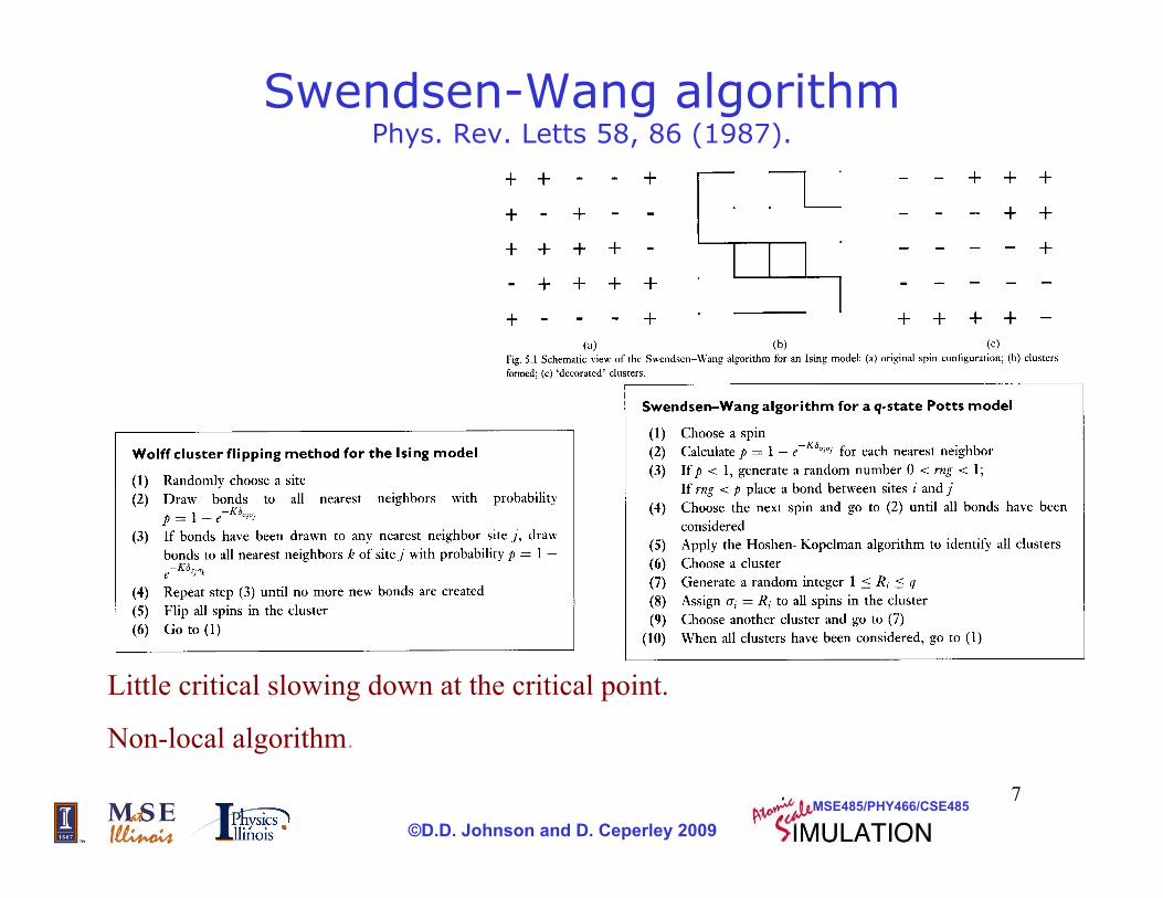
Swendsen-Wang algorithm Phys. Rev. Letts 58, 86 (1987).

Little critical slowing down at the critical point.

Non-local algorithm.


8

Correctness of cluster algorithm •  Cluster algorithm:

–  Transform from spin space to bond space nij

(Fortuin-Kasteleyn transform of Potts model)

–  Identify clusters: draw bond between only like spins and those with p=1-exp(-2J/kT)

–  Flip some of the clusters. –  Determine the new spins Example of embedding method: solve dynamics problem by

enlarging the state space (spins and bonds). •  Two points to prove:

–  Detailed balance joint probability:

–  Ergodicity: we can go anywhere How can we extend to other models?

Π σ ,n( ) = 1Z

1− p( )δni , j+ pδ

σ i−σ jδ

ni , j−1

i, j∏

p ≡1− e−2 J /kT

Trn Π σ ,n( ){ } = 1Z

eK δσ i−σ j

−1( )i , j∑


9

RNG Theory of phase transitions K. G. Wilson 1971

•  Near to critical point the spin is correlated over long distance; fluctuations of all scales

•  Near Tc the system forgets most microscopic details. Only remaining details are dimensionality of space and the type of order parameter.

•  Concepts and understanding are universal. Apply to all phase transitions of similar type.

•  Concepts: Order parameter, correlation length, scaling.


10

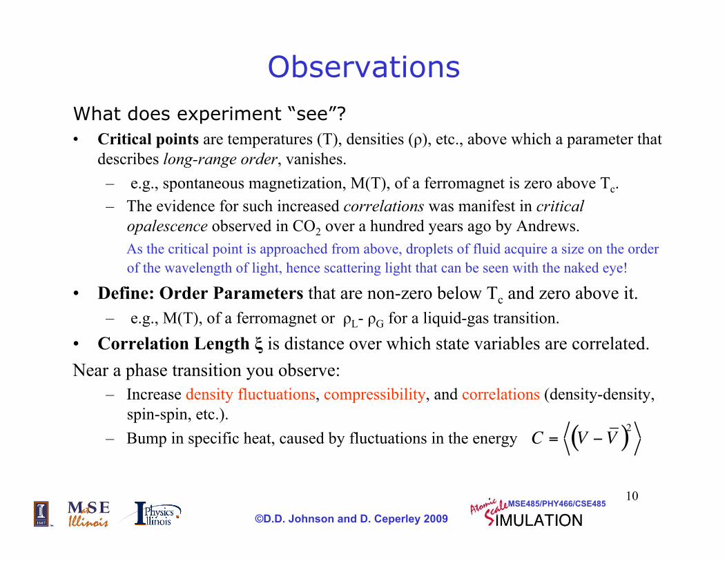
Observations What does experiment “see”?

•  Critical points are temperatures (T), densities (ρ), etc., above which a parameter that describes long-range order, vanishes. –  e.g., spontaneous magnetization, M(T), of a ferromagnet is zero above Tc. –  The evidence for such increased correlations was manifest in critical

opalescence observed in CO2 over a hundred years ago by Andrews. As the critical point is approached from above, droplets of fluid acquire a size on the order of the wavelength of light, hence scattering light that can be seen with the naked eye!

•  Define: Order Parameters that are non-zero below Tc and zero above it. –  e.g., M(T), of a ferromagnet or ρL- ρG for a liquid-gas transition.

•  Correlation Length ξ is distance over which state variables are correlated. Near a phase transition you observe:

–  Increase density fluctuations, compressibility, and correlations (density-density, spin-spin, etc.).

–  Bump in specific heat, caused by fluctuations in the energy


11

Blocking transformation

• Critical points are fixed points. R(H*)=H*.

• At a fixed point, pictures look the same!

•  Add 4 spins together and make into one superspin flipping a coin to break ties.

•  This maps H into a new H (with more long-ranged interactions)

•  R(Hn)=Hn+1


12

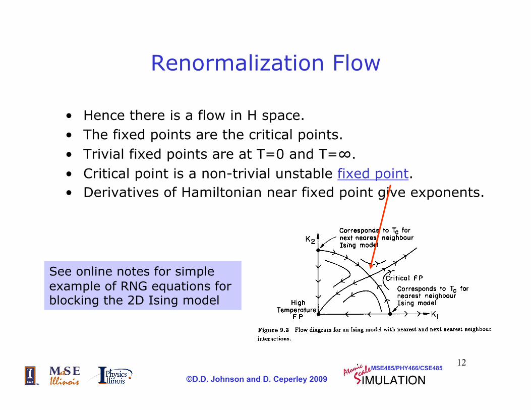
Renormalization Flow

•  Hence there is a flow in H space. •  The fixed points are the critical points. •  Trivial fixed points are at T=0 and T=∞. •  Critical point is a non-trivial unstable fixed point. •  Derivatives of Hamiltonian near fixed point give exponents.

See online notes for simple example of RNG equations for blocking the 2D Ising model


13

Universality •  Hamiltonians fall into a few general classes according to

their dimensionality and the symmetry (or dimensionality) of the order parameter.

•  Near the critical point, an Ising model behaves exactly the same as a classical liquid-gas. It forgets the original H, but only remembers conserved things.

•  Exponents, scaling functions are universal •  Tc Pc, … are not (they are dimension-full). •  Pick the most convenient model to calculate exponents •  The blocking rule doesn’t matter. •  MCRG: Find temperature such that correlation functions,

blocked n and n+1 times are the same. This will determine Tc and exponents.

G. S. Pawley et al. Phys. Rev. B 29, 4030 (1984).


14

Scaling is an important feature of phase transitions

In fluids, •  A single (universal) curve is found plotting T/Tc vs. ρ/ρc . •  A fit to curve reveals that ρc ~ |t|β (β=0.33).

–  with reduced temperature |t| =|(T-Tc)/Tc| –  For percolation phenomena, |t| |p|=|(p-pc)/pc|

•  Generally, 0.33 ≤ β ≤ 0.37, e.g., for liquid Helium β = 0.354.

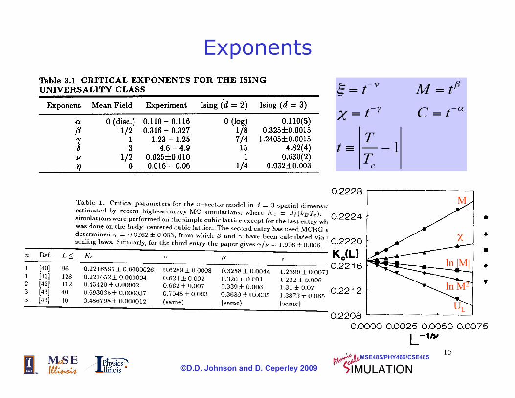
A similar feature is found for other quantities, e.g., in magnetism: •  Magnetization: M(T) ~ |t|β with 0.33 ≤ β ≤ 0.37. •  Magnetic Susceptibility: χ(T) ~ |t|-γ with 1.3 ≤ γ ≤ 1.4. •  Correlation Length: ξ(T) ~ |t|-ν where ν depends on dimension. •  Specific Heat (zero-field): C(T) ~ |t|-α where α ~ 0.1

α, β, γ, and ν are called critical exponents.


15

Exponents

M

χ

UL

ln |M|

ln M2


16

Primer for Finite-Size Scaling: Homogeneous Functions

•  Function f(r) “scales” if for all values of λ,

If we know fct at f(r=r0), then we know it everywhere!

•  The scaling function is not arbitrary; it must be g(λ)=λP, p=degree of homogeneity.

•  A generalized homogeneous fct. is given by (since you can always rescale by λ-P with a’=a/P and b’=b/P)

The static scaling hypothesis asserts that G(t,H), the Gibbs free energy, is a homogeneous function. •  Critical exponents are obtained by differentiation, e.g. M=-dG/dH


17

Finite-Size Scaling •  General technique-not just for the Ising model, but for other

continuous transitions. •  Used to:

–  prove existence of phase transition –  Find exponents –  Determine Tc etc.

•  Assume free energy can be written as a function of correlation length and box size. (dimensional analysis).

FN = Lγ f tL1/ν , HLβδ /ν( ) t ≡ 1−T / Tc

•  By differentiating we can find scaling of all other quantities •  Do runs in the neighborhood of Tc with a range of system sizes. •  Exploit finite-size effects - don’t ignore them. •  Using scaled variables put correlation functions on a common graph. •  How to scale the variables (exponent) depends on the transition in question. Do we assume exponent or calculate it?


18

Heuristic Arguments for Scaling

With reduced temperature |t| =|(T-Tc)/Tc|, why does ξ(T) ~ |t|-ν ?

•  If ξ(T) << L, power law behavior is expected because the correlations are local and do not exceed L.

•  If ξ (T) ~ L, then ξ cannot change appreciable and M(T) ~ |t|β is no longer expected. power law behavior.

•  For ξ (T) ~ L~|t|-ν, a quantitative change occurs in the system.

Scaling is revealed from the behavior of the correlation length.

Thus, |t| ~ |T-Tc(L)| ~ L-1/ν, giving a scaling relation for Tc.

For 2-D square lattice, ν=1. Thus, Tc(L) should scale as 1/L! Extrapolating to L=∞ the Tc(L) obtained from the Cv(T).


19

Correlation Length •  Near a phase transition a single length characterizes the

correlations •  The length diverges at the transition but is cutoff by the

size of the simulation cell. •  All curves will cross at Tc; we use to determine Tc.


20

Scaling example •  Magnetization of 2D Ising model •  After scaling data falls onto two curves

–  above Tc and below Tc.


21

Magnetization probability •  How does magnetization vary across transition? •  And with the system size?


22

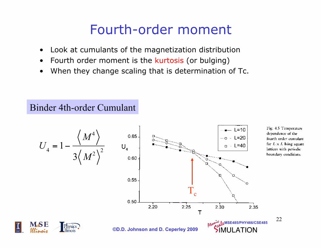
Fourth-order moment •  Look at cumulants of the magnetization distribution •  Fourth order moment is the kurtosis (or bulging) •  When they change scaling that is determination of Tc.

Tc

Binder 4th-order Cumulant


23

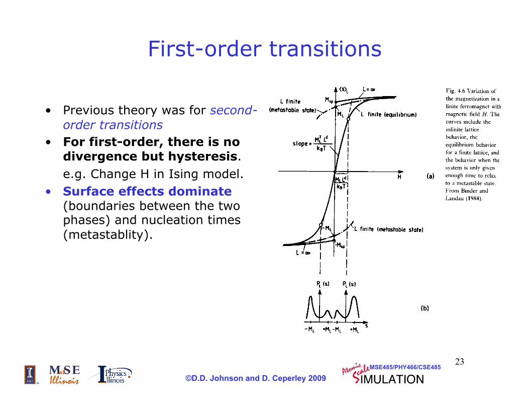
First-order transitions

•  Previous theory was for second-order transitions

•  For first-order, there is no divergence but hysteresis. e.g. Change H in Ising model.

•  Surface effects dominate (boundaries between the two phases) and nucleation times (metastablity).

phase transitions and finite-size scaling

Documents