Critical Notice:

Joseph Halpern, Actual Causality, Cambridge, MA, MIT Press 2016

Ian Rosenberg and Clark Glymour

Department of Philosophy

Carnegie Mellon University

Abstract

Halpern's Actual Causality is an extended development of an account of causal relations among

individual events in the tradition that analyzes causation as difference making. The book is

notable for its efforts at formal clarity, its exploration of "normality" conditions, and the wealth

of examples it uses and whose provenance it traces. Unfortunately, the various normality

conditions considered undermine the capacity of the basic theory to plausibly treat various cases

Halpern considers, and the unalloyed basic theory yields implausible results in simple cases of

overdetermination, which are not remedied by Halpern's probabilistic version of his theory or

unambiguously by the variety of normality conditions Actual Causality entertains.

Corresponding author: Clark Glymour, cg09@andrew.cmu.edu

1

1. Introduction

Theories of "actual causation" aim to provide an informative guide for assessing which events

cause which others in circumstances where almost everything else is known: which other events

occurred or did not occur, and how if at all the occurrence or non--occurrence (regarded as

values of a variable) of a particular event can depend on specific other events, or their absence,

also regarded as values of variables. The ultimate aim is a theory that can agreeably be applied in

causally fraught circumstances of technology, the law, and everyday life, where the identification

of relevant features is not immediate and judgements of causation are entwined with judgements

of moral or legal responsibility. Joseph Halpern's Actual Causality is the latest and most

extensive addition to this effort, carried out in a tradition that holds causation to be difference

making.

Actual Causality is notably valuable in providing a wealth of examples and carefully tracing their

provenance. Beyond articulation of (several) theories of actual causation, the book includes

guidance on how to model situations, and on legal and moral applications. A reader with a

critical eye will learn a great deal from it about the possibilities and difficulties of giving a clear,

quasi-formal account of judgements of causal relations among particular events. For those

interested in the subject, those are reasons enough to study and value the book. They will not,

unfortunately, find in it a satisfactory theory of actual causation, but they will find a challenging,

and in places frustrating, exploration of possibilities.

Any such theory meets two kinds of test cases, those from scientific and mechanical contexts

where the pertinent events, the dependences, and what differences are made by specific

interventions on component parts, are settled. Fault detection problems in engineering provide

such examples: when a machine of known design fails to produce the right output for an input,

there is a fact to the matter as to what component failures caused the wrong output, and what

interventions to replace them will restore the intended functioning. The very cover of Actual

Causality--depicting a Rube Goldbergish machine--suggests mechanical applications.

2

A formula for assessing actual causation that works smoothly for mechanics can grind against

intuition in examples drawn from the law and from everyday life, where judgements can vary

with descriptions of events and are confounded with moral sensibilities and epistemological

issues. It would be too much to expect a theory to handle all such cases in a manner that prompts

unanimous agreement, but we do expect a theory that unambiguously solves the cases it is

intended to treat and does not yield results that violate some of our most fundamental judgements

connecting causality and responsibility.

2. The Modified Definition of Causality:

Halpern provides a formal language for actual causation. He offers three distinct definitions of

causality, two based on previous proposals in collaboration with Pearl, and a "modified HP

definition." Halpern presents the modified version as his best, so we will here ignore the others.

In crudest form, the idea is that an event x--a happening or non-happening--that is a value of a

variable X, is a cause of an event y, a value of a variable Y, just if, were the value of X to be

different, the value of Y would be different, provided some things were to stay the same. That

basic inspiration is compromised at various points in Halpern's intricate discussion of

"normality."

Halpern gives a formal definition of "x actually causes φ (according to a model M with variables

V, for a context u):

3

AC1. (M, u) |= (X = x) and (M, u) |= φ. (23)

AC2(am). There is a set W of variables in V and a setting x’ of the variables in X’

such that:

if (M, u) |= W = w*, then (M, u) |= [X x’, W w*] φ (25)

AC3. X is minimal; there is no strict subset X’ of X such that X’ = x’ satisfies the

conditions AC1 and AC2, where x’ is the restriction of x to the variables in X. (23)

Here M, the model, is a pair <G, F>, where G is a directed (usually, acyclic) graph each of whose

vertices is a variable ranging over possible values of a particular event, e.g. "happens" coded as

1; or "does not happen" coded as 0, and F is a set of functions specifying the value of each

variable for each assignment of values to its parents in the graph. The function u assigns values

to the zero indegree variables in G, which, with F, determine unique values for all other variables

in G. (M,u) is the tuple of the causal model and the context, or total assignment of values to the

zero indegree variables and thus indirectly to all other variables in accord with F1. This can be

understood as the ‘actual world.’ X and W are sets of variables, and x and w are value

assignments that correspond to them. w* is the value of W in the actual world. The stylus "|="

1 A word on terminology. Halpern sometimes treats u as an assignment of a value to an

exogenous variable not represented in his or our causal graphs. This value then determines

the values of all zero-indegree variables in the graph, which in turn, through F, determine

the values of all other variables in the graph. Halpern omits this variable for situations that

can be adequately described just within the graph. Thus when he writes "endogenous"

what is intended may vary depending on the use of this variable. Where u is included, he

means all variables represented in the graph. Where it is excluded, he follows the more

usual terminology, and refers to only those variables in the graph that have positive

indegree. His use of "exogenous" varies similarly, meaning either just u, or those variables

in the graph with zero indegree respectively. Technically, the difference makes no

difference, but a careful reading of each scenario must be given in order to correctly

interpret Halpern’s meaning.

4

indicates semantic entailment. The formulae in square brackets indicate interventions that fix the

values of the upper case variables to the lower case values and should be read as if they were on

the left hand side of the entailment symbol. The interventions and assignments that satisfy

AC2(am) are said to be a "witness" to the actual causality of x provided x satisfies the other two

requirements. Note that while we will almost always discuss cases in which variables range over

two values, Halpern allows variables to have a larger range.

AC1 just says that the actual world satisfies the value assignment of the proposed cause and

effect. In other words, X = x cannot be a cause of φ unless x is the actual value of X and φ is true.

AC3 is a straightforward minimality constraint on the cause: X and x can be vectors (or sets or

lists), and minimality requires than no vector whose components are a proper subset of those of x

satisfies the other conditions. AC2(am) is the real substance of the definition, and is the most

complex criterion. In Halpern’s words it says “we can show the counterfactual dependence of φ

on X by keeping the variables in W fixed at their actual values” (25). We just need to find some

set, possibly empty, of variables to hold at their actual values. With this set of variables fixed, x

must be a "but-for" cause of φ: in that circumstance, change in the value of X would change the

truth value of φ. When x has more than one component but satisfies AC1- AC3, each component

of x is a partial cause of φ. Note that in AC2(am) does not allow fixing any variable other than X

at any value other than its actual one.

Halpern extends his theory to include probability relations. He takes probabilities that might be

given by a contingency table specifying the probability of each value of each variable, X,

conditional on each assignment of values to the parents of X in the graph, as measures on

deterministic cases, or as Halpern says "pulled out," and his deterministic account applied in

each case, with resulting probabilities.2

2 We do not understand one of Halpern's remarks about his probabilistic version. Turning

the joint probabilities of events contingent on values of their direct graphical parents into

measures on deterministic models is straightforward, but Halpern (p. 47) says the resulting

probabilities are not to be understood as probabilities conditional on models in which the

the parents have such and such values, but rather are to be understood as "interventions,"

writing "For example, the fact that Suzy's rock hits with probability .9 does not mean that

5

3. Mechanics and Overdetermination

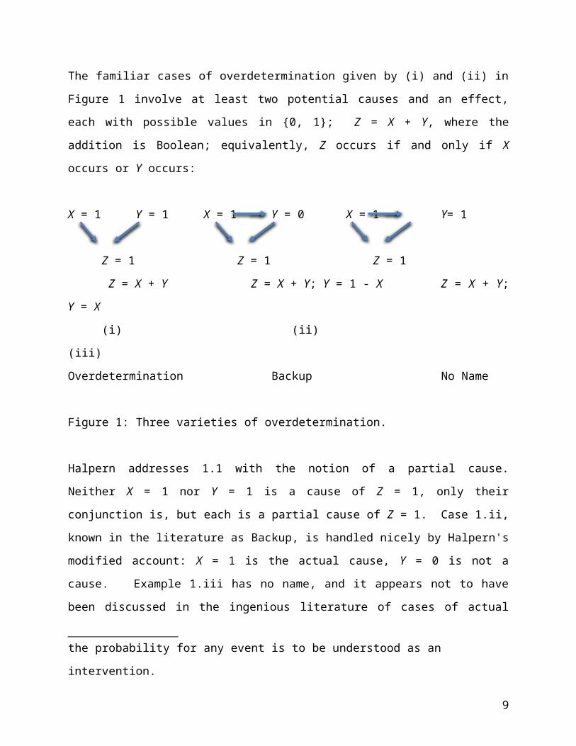
The familiar cases of overdetermination given by (i) and (ii) in Figure 1 involve at least two

potential causes and an effect, each with possible values in {0, 1}; Z = X + Y, where the addition

is Boolean; equivalently, Z occurs if and only if X occurs or Y occurs:

X = 1 Y = 1 X = 1 Y = 0 X = 1 Y= 1

Z = 1 Z = 1 Z = 1

Z = X + Y Z = X + Y; Y = 1 - X Z = X + Y; Y = X

(i) (ii) (iii)

Overdetermination Backup No Name

Figure 1: Three varieties of overdetermination.

Halpern addresses 1.1 with the notion of a partial cause. Neither X = 1 nor Y = 1 is a cause of Z

= 1, only their conjunction is, but each is a partial cause of Z = 1. Case 1.ii, known in the

literature as Backup, is handled nicely by Halpern's modified account: X = 1 is the actual cause,

Y = 0 is not a cause. Example 1.iii has no name, and it appears not to have been discussed in the

ingenious literature of cases of actual causation; Halpern does not consider it. Halpern's theory,

however, is unequivocal: X = 1 is a cause of Z = 1, but Y = 1 is not a cause, not even a partial

cause. Halpern (personal communication) endorses this result. In mechanical cases, Halpern's

the probability of Suzy's rock hitting conditional on her throwing is .9, rather it means that

if there is an intervention that results in Suzy throwing, the probability of Suzy's rock

hitting is .9" He justifies this remark with the following: "The probability of rain

conditional on a low barometer reading is high. However, intervening on the barometer

reading, say by setting the needle to point to a low reading, does not affect the probability

of rain." The first quoted sentence is odd, since in the example the probabilities are the

same in either case, intervention or conditioning. The second quoted sentence is of course

true; we are perplexed as to what it has to do with Halpern's claim that the probability for

any event is to be understood as an intervention.

6

solution to 1.iii yields what would sometimes be called in the fault detection literature a "root

cause." If X were a component stuck at 1 with the result that Y = 1 and Z = 1, and the desired

behavior is that Z = 0, a repair would be to replace X with a component that is not stuck at 1. In

this mechanical case, Halpern's theory gets things right.

4. Life, Death and Probability

Consider another interpretation of the causal system of figure I.iii. An obedient gang is ordered

by its leader to join him in murdering someone, and does so, all of them shooting the victim at

the same time, or all of them together pushing the plunger connected to a bomb. The action of

any one of the gang would suffice for the victim's death. If responsibility implies causality,

whom among them is responsible? Were you among the jury, whom would you convict? What

ought the Hague Court to do in cases of subordinates sure to obey orders? Halpern's theory says

the gang leader and only the gang leader is a cause of the victim's death. This is a morally

intolerable result; absent a plausible general principle severing responsibility from causation, any

theory that yields such a result should be rejected.

What if the action of the superior does not necessitate the action of the subordinate, but only

makes it probable? In that case, the result on Halpern's theory of probabilistic causality is that the

probability that Y = 1 is a cause of Z = 1 is zero! Halpern's strategy is:

"...to convert a single causal setting where the equations are probabilistic to a probability over

settings, where in each causal setting the equations are deterministic. This, in turn, will allow me

to avoid giving a separate definition of probabilistic causality. Rather, I will use the definition of

causality already given for deterministic models and talk about the probability of causality, that

is, the probability that A is a cause of B."(48)

Suppose then that we alter case 1.iii so that the probability that Y = 1 when X = 1 is p, leaving the

dependence of Z on X and Y unchanged. Then, following Halpern's probability recipe, we have

for p fraction of the cases X = Y = Z = 1, and 1-p fraction of cases in which X = Z = 1 and Y = 0.

Applying Halpern's theory to each of the p cases yields that Y = 1 is not a cause of Z = 1, as

7

before. But the 1- p cases where X =1 and Y = 0 and Z = 1 are instances of Backup, figure i.ii,

for which Halpern's deterministic theory also yields that the value of Y is not a cause of Z = 1.

Thus, whatever p may be, Halpern's theory says the probability that the value of Y is an actual

cause of Z = 1 is zero.

We will consider subsequently whether any of Halpern's proposed normality conditions rescue

his theory from this and other consequences.

5. The Curious Case of Billy and Suzy

Halpern analyzes the following example repeatedly throughout his book to compare different

formulations of causation and normality, so we will give it in full detail. The story is simple;

Billy and Suzy both throw rocks at a bottle, Suzy just before Billy. Suzy’s rock hits the bottle,

smashing it, but had her rock not hit it, Billy’s would have, to the same effect. The variables

“Suzy Throws”, “Billy Throws”, and “Bottle Smashes” are represented as ST, BT, and BS

respectively. Halpern adds variables BH and SH for Billy or Suzy’s rock actually hitting the

bottle. Whether Suzy’s rock hits depends only on her throwing since she is a good shot, but

Billy’s rock will only hit the bottle if he throws and Suzy’s rock doesn’t hit. Halpern refers to

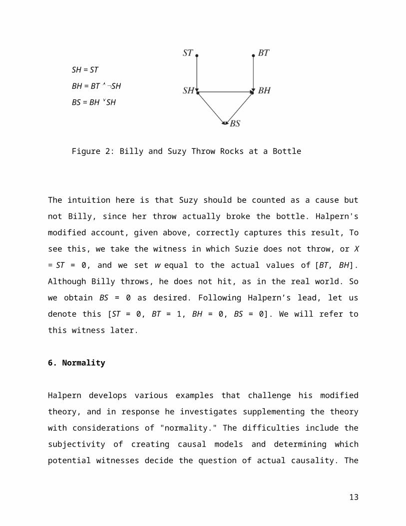
this causal model as M’RT, and it appears in the following form (31):

SH = ST

BH = BT SH

BS = BH SH

Figure 2: Billy and Suzy Throw Rocks at a Bottle

The intuition here is that Suzy should be counted as a cause but not Billy, since her throw

actually broke the bottle. Halpern's modified account, given above, correctly captures this result,

8

To see this, we take the witness in which Suzie does not throw, or X = ST = 0, and we set w

equal to the actual values of [BT, BH]. Although Billy throws, he does not hit, as in the real

world. So we obtain BS = 0 as desired. Following Halpern’s lead, let us denote this [ST = 0, BT =

1, BH = 0, BS = 0]. We will refer to this witness later.

6. Normality

Halpern develops various examples that challenge his modified theory, and in response he

investigates supplementing the theory with considerations of "normality." The difficulties

include the subjectivity of creating causal models and determining which potential witnesses

decide the question of actual causality. The introduction of normality also serves the ambition to

make finer distinctions, for example between a cause and a "background condition." In situations

where his original definition cannot differentiate among possible causes, normality allows

Halpern to select among them in order to gain better agreement with intuition. He offers in

sequence several accounts of normality, each designed to deal with a counterexample to the

previous one. In the course of these changes some of the revisions violate the restrictions of the

modified account, and some lose the basic intuition of the modified account--an actual cause is

an event that, were it not to happen and things otherwise stay pretty much as they are, the effect

would not happen. His discussion is intricate and inevitably so are our assessments.

Halpern recognizes that "normality" is often vague, or at least ambiguous. A situation would be

perfectly normal if all of the variables took on their default values, or those which we expect

with no other information. Related to normality is the notion of typicality, which can be

understood as statistical prevalence or as a characteristic trait of an object. Moral or legal norms

can also be used to decide which value a variable should ‘normally’ take. Halpern uses all of

these ideas to help evaluate the normality of a world or variable assignment (p. 78). Beyond

these mostly qualitative considerations, Halpern acknowledges that measuring normality cannot

be done easily, although in the end he offers a counting principle.

Halpern’s allows that there may be two worlds s and s’ whose relative normality is

incomparable.

9

The fact that s and s’ are incomparable does not mean that s and s’ are equally

normal. We can interpret it as saying that the agent is not prepared to declare

either s or s’ as more normal than the other and also not prepared to say that they

are equally normal; they simply cannot be compared in terms of normality. (81)

Even worlds that are intuitively comparable might be so close to each other in normality that the

judgment of equi-normality, or not, would be entirely subjective. To avoid this issue Halpern

requires that an inequality in normality should be interpreted as a very large difference. “…to the

extent that we are thinking probabilistically, we should interpret u > u’ as meaning “u is much

more probable than u’ ” (97).

Halpern's normality conditions are constraints on witnesses to an actual cause, that is on

counterfactual situations in which a potential causal variable and a potential effect variable both

change value. Since he proposes various combinations of accounts, counting the number of

proposed theories of normality is not straightforward, but the following seem basic:

1. A witness is a circumstance at least as normal as the actual circumstance.

2. A witness is a circumstance than which there is no other more normal of all possible

alternative circumstances.

3. A witness is a circumstance whose events are the most probable.

4. A witness is a circumstance that is produced with the fewest number of interventions on

the actual circumstance.

An intervention on a variable changes its value or fixes its value at its actual value, possibly

violating some of the constraints, F. Values of variables "downstream" from an intervened value

(graphically, descendants) take on new values, or remain the same, in accordance with F and the

values specified by the interventions.

Observe that variants 2, 3 and 4 change the framing from the modified criterion without

normality. In the modified criterion, and with normality condition 1, candidate witnesses were

assessed for a candidate actual cause without regard to candidate witnesses for other candidate

10

causes. But in 2, 3 and 4, potential witnesses for different potential causes are in competition,

and only a witness and actual cause are allowed than which there is no more normal witness for

any potential cause.

6. 1 Halpern’s First Approach to Normality

Consider the case of a camper dropping a match and starting a forest fire. The fire would not

start unless there were oxygen available, but we would not ordinarily cite the presence of oxygen

as a cause. Halpern deals with this sort of case by appeal to normality. His first approach to

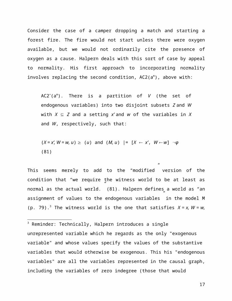
incorporating normality involves replacing the second condition, AC2(am), above with:

AC2+(am). There is a partition of V (the set of endogenous variables) into two

disjoint subsets Z and W with X Z and a setting x’ and w of the variables in X

and W, respectively, such that:

(X = x’, W = w, u) (u) and (M, u) |= [X x’, W w] φ (81)

This seems merely to add to the “modified” version of the condition that “we require the witness

world to be at least as normal as the actual world.” (81). Halpern defines a world as “an

assignment of values to the endogenous variables” in the model M (p. 79).3 The witness world is

the one that satisfies X = x, W = w, and φ. In the case of a camper dropping a match and

starting a forest fire, we can construct the witness for oxygen as a cause by intervening and

eliminating the oxygen, but an Earth now without oxygen is not at least as normal as reality (82).

So, by the normality condition, we cannot find that oxygen was a cause of the forest fire. Thus

normality helps us limit the scope of our causal attributions and thereby helps us select the more

intuitively reasonable cause.

3 Reminder: Technically, Halpern introduces a single unrepresented variable which he

regards as the only "exogenous variable" and whose values specify the values of the

substantive variables that would otherwise be exogenous. This his "endogenous variables"

are all the variables represented in the causal graph, including the variables of zero

indegree (those that would customarily be deemed "exogenous").

11

There is, a troubling ambiguity in AC2+(am). In AC2(am) w is w*, the actual value of W. There is

no asterisk on w in AC2+(am) and Halpern does not comment on the absence. So we do not

know whether in producing a witness for x as an actual cause, interventions are allowed that fix

other variables at other than their actual values. However, in example 3.26 (84), Halpern

contrasts this normality condition for his modified definition, AC2(am), with the same normality

condition applied to Halpern-Pearl theories, observing that the latter give different results than

the modified definition because they do not restrict w to actual values. So we take it that in

AC2+(am). w should be w*, the actual values. In later versions of normality Halpern seems to

forget this condition.

If we incorporate normality as Halpern initially proposes--the witness case must be at least as

normal as the actual case--we lose the result that Suzy is a cause of the bottle breaking and Billy

is not. Halpern writes:

Suppose we declare the world where Billy throws a rock, Suzy doesn’t throw, and

Billy does not hit abnormal. This world was needed to show that Suzy throwing is

a cause according to the modified HP definition. Thus, with this normality

ordering ST = 1 is not a cause; rather, ST = 1 ^ BT = 1 is a cause, which seems

inappropriate (84).

Halpern’s supposition that it would be abnormal for Suzy not to throw, Billy to throw and Billy

not to hit seems quite reasonable. He has thus far assumed that Billy would hit the bottle had not

Suzy hit it first. This relationship between the two throws is, in fact, the essential feature of this

example, and the reason it was an interesting scenario to explore in the first place. But Halpern

seems to immediately reverse course to preserve his interpretation’s validity. Just lines later he

claims “The witness world where BT = 1, BH = 0, and ST = 0 does not seem so abnormal, even

if it is abnormal for Billy to throw and miss in a context where he is presumed accurate” (84).

We seem to have a case of the philosophical argument "I need it to be the case that p; therefore,

p."

12

But Halpern is not so sanguine: the first normality condition is consistent with none of the events

being actual causes if no candidate witness is as normal as the actual case. And Halpern notes

correctly that this first treatment of normality delivers unintuitive results in straightforward

scenarios where only the most normal series of events plays out. In the case of a gardener

watering her plants, the gardener not caring for her garden is less normal than reality, so that she

waters the plants is not a cause of the plants survival. So, to graded causation.

6.2 Graded Causation

Halpern introduces a new notion, graded causation. Instead of judging whether a variable is the

cause of an outcome in a binary fashion, potential causes can be compared based on the

normality of their witness worlds, and the potential cause (or causes) with the most normal

witness is selected. Since the world in which the gardener does not water her plants is more

normal than, say, the worlds in which soil does not provide nutrients, or the sun does not shine,

the gardener watering her plants is the cause of their survival. Notice that we are now in a

different regime from the plain modified account: in the plain modified account, and in the first

version of normality, each potential cause is assessed by itself: with graded causation, potential

causes are in competition.

Returning to Billy and Sally, Halpern’s graded approach also fails. Suzy throws first and breaks

the bottle, but the graded approach to normality fails to deem her a cause for two reasons: the

most normal witness to Suzy not being the cause of the bottle breaking is the circumstance in

which neither of them throw; and as before, by AC2(am) there is no allowable witness to Suzy's

throw as an actual cause of the bottle breaking. We have the same problem as with the first

normality proposal: Billy's and Sally's throw is the conjunctive cause. Halpern goes on to

introduce a third alternative approach to incorporating normality.

6.3 Graded Causation with Probabilities of Events

This the approach differs from the first primarily in that he puts the normality ordering on sets of

contexts instead of worlds. A context “can be identified with a complete assignment,” that is, an

13

assignment of values to all of the variables (80). Here is the formalization, fixing the causal

model, M and using a pre-ordering of normality of contexts for M and interventions on variables

in M :

There is a partition of V (the set of endogenous variables) into two disjoint subsets

Z and W with X Z and a setting x’ and w of the variables in X and W,

respectively, such that:

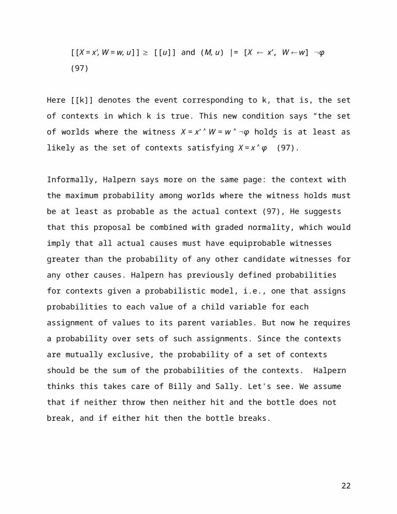
[[X = x', W = w, u]] [[u]] and (M, u) |= [X x’, W w] φ (97)

Here [[k]] denotes the event corresponding to k, that is, the set of contexts in which k is true.

This new condition says “the set of worlds where the witness X = x' W = w φ holds is at

least as likely as the set of contexts satisfying X = x φ” (97).

Informally, Halpern says more on the same page: the context with the maximum probability

among worlds where the witness holds must be at least as probable as the actual context (97), He

suggests that this proposal be combined with graded normality, which would imply that all actual

causes must have equiprobable witnesses greater than the probability of any other candidate

witnesses for any other causes. Halpern has previously defined probabilities for contexts given a

probabilistic model, i.e., one that assigns probabilities to each value of a child variable for each

assignment of values to its parent variables. But now he requires a probability over sets of such

assignments. Since the contexts are mutually exclusive, the probability of a set of contexts

should be the sum of the probabilities of the contexts. Halpern thinks this takes care of Billy and

Sally. Let's see. We assume that if neither throw then neither hit and the bottle does not break,

and if either hit then the bottle breaks.

Suzy Throws Billy Throws Suzy Hits Billy Hits Bottle Shatters Probability

1 1 1 0 1 p

1 1 0 1 1 q

1 1 0 0 0 r

1 0 1 0 1 s

14

1 0 0 0 0 t

0 1 0 1 1 u

0 1 0 0 0 v

0 0 0 0 0 z

ST = 0 and BS = 0 are necessary elements of the witness context for Suzy's throw to be a cause.

If the fixed values w of the witness must be the actual values of W, then we are restricted once

more to the context in the sixth row of the table, where the bottle shatters, and, as before, we do

not have a witness to Suzy as a cause: if Suzy does not throw, the probability is 1 that the bottle

shatters. If W is not required to have its actual value, the probability that Suzy does not throw

and the bottle does not shatter is v + z, which must be greater than p for Suzy's throw to cause

the bottle to shatter. It comes out right for Halpern only if probably Billy does not throw or

probably Billy is a lousy shot. The second disjunct rather loses the tension of the example.

Halpern claims his reasoning extends even to a modified scenario in which Billy is a rock-

throwing machine. “Although it may be unlikely that the rock-throwing machine does not throw

or throws and misses, it may not be viewed as all that abnormal” (98). We are forced to ask how

unlikely an event must be for it to cross the threshold into abnormality. Halpern himself admits

that the elements of the set violate statistical typicality, and they certainly go against any kind of

defaults that a reasonable person might hold. In his very own explanation of this approach he

says the set in which the witness holds “must be at least as likely” as the set in which reality

holds. His consideration of the rock-throwing machine seems to directly contradict this.

Halpern’s normality considerations so far actually make his definition perform worse, and on an

example he himself has used as a key test of his own definition. The Billy and Sally case comes

out neatly on the plain modified account; it comes out as an ad hoc mess on the graded

probability account, and only gets that far by ignoring the letter of AC2(am). But if we ignore the

letter of AC2(am), and allow interventions that do not fix variables at their actual values, Backup

no longer turns out right on the modified account and only turns out right on the graded and

graded probability accounts if we arbitrarily add ad hoc assumptions about normality or

probability.

15

6.4 The ABC Switch and Counting Interventions

Halpern presents another example, the ABC switch, for which he allows that his previous

normality considerations fail, and then introduces still another method of considering normality.

The new example involves a system of two switches connected to a light bulb, operated by two

individuals, A and B. We will again give the situation in full detail, starting with Halpern’s

description:

A and B both each control a switch. There are wires going from an electricity

source to these switches and then continuing on to C. A must first decide whether

to flip his switch left or right, then B must decide (knowing A’s choice). The

current flows, resulting in a bulb at C turning on, iff both switches are in the same

position. B wants to turn on the bulb, so flips her switch to the same position as A

does, and the bulb turns on. (100)

Schematically:

B = A = 1; C = 1 iff A = B

Figure 3. Light Switch

Halpern claims “intuition suggests that A’s actions should not be viewed as a cause of the C bulb

being on, whereas B’s should” (100). We cannot achieve this result with the modified HP

definition alone. If we hold B constant at its actual value (1) and intervene on A, we get A is a

16

cause. Similarly for B. So we obtain both A and B as actual causes of the outcome. Looking to

the original approach to normality, we get no help. “Taking u to be the context where A = 1, both

[A = 0, B = 1, u] and [B = 0, u] seem less normal than u, and there seems to be no reason to

prefer one to the other, so graded causality does not help in determining a cause” (101). The third

approach also fails. “Similarly, for the alternative approach, both [[A = 0 ^ B = 1 ^ C = 0]] and

[[B = 0 ^ C = 0]] are less normal than either [[A = 1 ^ C = 1]] or [[B = 1 ^ C = 1]]. Again, there

is no reason to prefer B = 1 as a cause.” (101). So Halpern’s concludes that his previous

approaches to incorporating normality offer no help in this scenario.

In response to this new difficulty, Halpern introduces a new technique for incorporating

normality. “Rather than considering the “absolute” normality of a witness, we can consider the

change in normality in going from the actual world to the witness and prefer the witness that

leads to the greatest increase (or smallest decrease) in normality” (102). To measure this change

in normality, Halpern relies on the structural equations and the number of interventions required

to create the witness context. He does not say whether we are to weight these two kinds of

interventions differently or equally.

Now we take the change from the world where both A = 1 and B = 1 to the world

where A = 1 and B = 0 to be smaller than the one to the worlds where A = 0 and

B = 1 because the latter change involves changing what A does as well as

violating normality (in the sense that B does not act according to the equations),

while the former change requires only that B violate normality. This gives us a

reason to prefer B = 1 as a cause. (102)

Halpern's story is not entirely clear because there is no initial state given for A, B and C. So

suppose initially A and B have some third neutral value, there is no current, and the light is off.

A is set to 1 and B is set to 1 and the light turns on. If A had been set to 0 then, keeping the

value of B at its actual value, 1, in accord with AC2(am) the light would not be on and we would

have a witness to A = 1 as a cause. If B had been set to 0 then the light would not be on, also in

accord with AC2(am), and we would have a witness to B = 1 as a cause. The former requires two

interventions, the latter 1, so B = 1 wins the causality challenge.

17

We have now lost the entire spirit of the plain modified condition. Not only are candidate causes

competing, but application of the very idea of AC2(a'') that other variables may be fixed at their

actual values counts against a witness: each variable fixed at its actual value counts as an

intervention, so the more the witness is required to agree with the actual case, the worse the

witness!

.

What does this new account of normality do for previous examples? There are two possible

witnesses for Suzy alone being an actual cause: [ST = 0, BT = 1, BH = 0, BS = 0] requires two

interventions on the actual state of affairs; and [ST = 0, BT = 0, BH = 0, BS = 0] also requires two

interventions. But the latter is also a witness for Billy being the cause. Either both throws are

causes or there is no decision.

If we use only the number of interventions to compare normality, we create all sorts of confusing

results. Consider the forest fire example again. Removing the oxygen from the forest, or

preventing the hiker from dropping a match both only take one intervention. Of course, one of

these "interventions" is more plausible than the other, and we might say more probable than the

other. So is the idea that we count interventions and then use only the most probable?

6.5 The First Example, with Normality

We consider whether Normality helps with the example with which we began. Our model is

graphically similar to that of the light switch example but with a different functional relation. We

have variables Gang Leader Shoots (GS), Henchman Shoots (HS), Enemy Dies (ED). The enemy

dies if either the gang leader or the henchman shoots, but the henchman will only shoot if and

only if the gang leader does.

HS = GS

ED = GS HS

18

Figure 4: Gang Leader and Gang Members Jointly Kill

Using the plain modified definition, the gang leader caused the death of the enemy, as expected.

We cannot create a witness for henchman being a cause. If we set HS = 0, we still get ED = 1

unless we also intervene to change GS = 1 to GS = 0, which the modified HP definition does not

allow. We can construct a witness for both being a cause, but given the minimality condition, we

must reject this as a cause. So the henchman cannot even be considered part of the cause. We

have seen that probability does not prevent this result. In section 6.2, Halpern proposes a

measure of degree of blame invoking his probabilistic account. By that measure, the Henchman

is blameless.

Working through the normality considerations, we get results that are unacceptable or various

although they are a bit difficult because, well, killing people is not normal. With the initial

approach or the graded approach we still obtain GS = 1 is a cause, since, given the moral and

legal norms concerning murder, the world in which the gang leader doesn’t shoot is at least as

normal as the supposed actual case. We have no clear idea what to do for a witness for the gang

leader as a cause. There are worlds in which he and the gang leader both shoot and miss, worlds

in which the gang member does not shoot but the gang leader does and misses, and the world in

which neither of them shoot. We have no idea as to the probabilities. The last--neither of them

shoot--is the same witness as for the gang leader. Are they both then causes, or only the gang

leader? What happens when we count interventions? An intervention that changes the gang

leader's order and firing while retaining all of the functional dependencies (F), so that none of the

gang, including the leader, fire, and the intended victim survives, is a witness to the gang leader

as a cause with one intervention. In order to provide a witness for the gang member as cause,

19

both the gang member and the gang leader must be intervened on. But maybe not--maybe the

single intervention on the gang leader, which results in the gang member not shooting, counts as

a witness for the gang member and the gang leader as the cause, so the gang member is a partial

cause. But that would seem to violate the mimimality requirement of AC(2m) and would also

violate a strict reading of AC(2m) which requires in a witness an intervention to directly change

the actual cause. Halpern's brief discussion (102) provides us with no guidance.

7. Results

If the reader is lost in the tangle of normalities, our sympathies. We’ have now considered

several examples, each with a distinct causal structure and applicable norms. The results often

disagree. Here is our summary of the examples and their results for the several accounts of

normality. We count a criterion as a success (marked with an O) for a case if its application

unequivocally agrees with intuition, as defined within the example.

20

Example

Forest Fire GardenerRock

ThrowingSwitches

Gang

Execution

Billy +

Suzie

Modified

DefinitionO O

O

Cau

salit

y M

odel

Normality

on WorldsO

Graded

CausationO O

Probability

of Sets of

Contexts

O O

# Changes

in

Normality

O

14. Conclusion

There are some serious issues with Halpern’s theory. Although the modified definition is clean

and, given the presuppositions of actual causality theories, unambiguous, and captures the

intuition on some difficult cases, it fails as a general tool to determine actual causality.

Normality, as a qualitative consideration, seems at first to help, and Halpern is able to create a

seemingly intuitive formalization of its application to causal models. Indeed, it does put useful

restrictions on some examples, restrictions that allow us to differentiate between confusing

potential causes. But when this formalization fails to correct some problem cases, normality

turns into a quagmire. Halpern responds by creating another proposal and then another and

another and another. These successive considerations, with increasing vagueness or ambiguity,

fail to correctly interpret the examples that their predecessors were created to address, and,

what’s more, all of them fail on the canonical rock-throwing example that the plain modified

definition successfully interpreted. On the simple, morally salient example with which we

21

began, the basic modified criterion fails, recourse to probability fails, and supplements with

normality conditions fail or are obscure. Worse, perhaps, without notice the framework of the

plain modified account is eroded and in a central respect even reversed. What we are left with is

an imperfect definition of actual causality together with a set of ad hoc corrections, none of them

satisfactory. The discussions of responsibility and blame signal that Halpern intends his theory to

be a serious guide in law and moral appraisal. For reasons indicated, we think that would be a

very bad thing.

Notwithstanding our hope that the theory never reaches into the practice of justice, and our

conclusion that no coherent, adequate theory of actual causation emerges, a lot can be learned

from Halpern's book. The variety of examples and proposals considered, and the subtleties of

their problems, should be a caution to anyone attempting a theory of actual causality. In that

service, Actual Causality deserves to become a standard but not an icon.

22