phy315 manual 2

7/30/2019 Phy315 Manual 2

http://slidepdf.com/reader/full/phy315-manual-2 1/78

LABORATORY MANUAL

(2012-2013)

MODERN PHYSICS LABORATORY

DEPARTMENT OF PHYSICS

INDIAN INSTITUTE OF TECHNOLOGYKANPUR-208016

7/30/2019 Phy315 Manual 2


Phy315: Modern Physics Laboratory

The laboratory course focuses on the experiments that led to the development of quantum mechanics including

determination of fundamental constants and illustration of some of the significant modern phenomena of physics.

It consists of about 15 different experiments of which at least six are compulsory. The experiments determine

some of the fundamental constants (Planck constant, e/m of electron, gravitational constant, Rydberg constant,

Boltzmann constant) or quantitatively demonstrate some of the concepts (quantum analog, Single photoninterference) and applications (Thermionic emission, Solar Cells) of quantum physics. Also there are

experiments that illustrate applications of thermodynamics (Johnson Noise, thermoelectric effect and Peltier

effect), and non-linear dynamics (chaos). The lectures consist of introduction to error analysis and essential tools

of modern experiments (vacuum and low temperatures), discussion of experiments leading to quantum

mechanics and a brief introduction to other experiments carried out in the

The laboratory runs twice for three hours in every week. We do allow students to prepare reports off the lab hours,

however, we'll not assign a new experiment unless the report of one experiment before the last one is received.

Thus at most one report backlog is allowed at any given time. A timely submission of the lab report helps inmaintaining the quality of the report. This manual should help you in preparing for the lab before you start the

experiment. We expect you to go through the write-up corresponding to your experiment before coming to the lab

to perform the experiment.

You will be provided with write-ups containing instructions on various experiments. You are also encouraged to read

the matter from the references (if any) given in the write-ups or suggested by your instructor.

On reaching the laboratory you should check the apparatus provided and ascertain if there are any shortages or

malfunctions. Set up the equipment in accordance with the instructions. Proceed carefully and methodically.

Remember that scientific equipments are expensive and quite susceptible to damage. So handle them carefully. If theapparatus is too complicated please ask the Instructor/TA or Lab staff to inspect it before you proceed with the actual

experiment.

It is more important to see what result you get with given apparatus rather than what is the correct result. The

apparatus given to you is capable of a certain accuracy and your result may be completely acceptable even if it differs

from the correct result. Further, you must learn to do things on your own even if you make mistakes some time.

In case results are to be found graphically; each graph should occupy one complete sheet; the information as to

quantities plotted, scale chosen and units should be mentioned clearly on each graph.

Following is the recommended format of the Report:

Lab reports are to be submitted before beginning a new experiment (at most one backlog allowed). The students are

expected (but not required)to spend about two turns on one experiment. This is an experimental course and we test the

originality and systematicness in carrying out the experiment and reporting the data, and thoroughness in analyzing

them to reach the appropriate result. It 's a good practice to keep a separate lab-book with raw data and a photocopy of

the relevant data pages should be attached to the report. The report may be divided into the following sections:

1. Your name (and partner's name), roll number, instructor‘s name, date title or the experiment.

2. Aim/goal (no abstract).

3. Theory (Brief) or principle

7/30/2019 Phy315 Manual 2


4. Procedure/apparatus/method/schematics

5. Data /observations (However ugly, show the raw data)

6. Graphs/ Analysis, and calculations (includes error analysis)

7. Result and errors/conclusions

8. Suggestions/Precautions/Difficulties faced/discussion/comments

Remember highest weightage in a report is given to points 5 and 6 as listed above. Also a hand written report is

recommended over the computer printout (other than the graphs).

Project:

In the last one month of the semester after each group has finished a minimum required number of experiments a

small project has to be chosen by student after brief literature search (eg., American Journal of Physics). These may be

carried out in research labs, using central facilities or some simple experiments may be set-up in 315 lab itself.

7/30/2019 Phy315 Manual 2


ERROR ANALYSIS

―To, Error is human; to evaluate and analyse the error is scientific‖.

Introduction: Every measured physical quantity has an uncertainty or error associated with it. An

experiment, in general, involves (i) direct measurement of various quantities (primary measurements)

and (ii) calculation of the physical quantity of interest which is a function of the measured quantities.

An uncertainty or error in the final result arises because of the errors in the primary measurements

(assuming that there is no approximation involved in the calculation).For example , the result of a

recent experiment to determine the velocity of light (Phys. Rev. Lett. 29 , 1346(1972)was given as

C = (299.792.456.2± 1.1) m/sec

The error in the value of C arises from the errors in primary measurements viz., frequency and

wavelength.

Error analysis therefore consists of (i) estimating the errors in all primary measurements, and (ii)

propagating the error at each step of the calculation. This analysis serves two purposes. First, the error

in the final result (± 1.1 m/sec in the above example) is an indication of the precision of the

measurement and, therefore an important part of the result. Second, the analysis also tells us which

primary measurement is causing more error than others and thus indicates the direction for further

improvement of the experiment.

For example ,in measuring ‗g‘ with a simple pendulum, if the error analysis reveals that the errors in ‗g‘

caused by measurements of 1 (length of the pendulum) and T (time period) are 0.5 cm/sec2

and 3.5 cm/

sec2

respectively, then we know that there is no point in trying to devise a more accurate measurement

of 1. Rather, we should try to reduce the uncertainty in T by counting a larger number of periods or

using a better device to measure time. Thus error analysis prior to the experiment is an important aspect

of planning the experiment.

Nomenclature:

(i) ‗Discrepancy‘ denotes the difference between two measured values of the same quantity.

(ii) ‗Systematic error s‘ are errors which occur in every measurement in same way- often in the same

direction and of the same magnitude – for example, length measurement with a faulty scale. These

errors can in principle, be eliminated or corrected for.(iii) ‗Random error s‘ are errors which can cause the result of a measurement to deviate in either

direction from its true value. We shall confine our attention to these errors, and discuss them under two

heads: estimated and statistical errors.

II Estimated Errors

Estimating a primary error: An estimated error is an estimate of the maximum extent to which a

measured quantity might deviate from its true value. For a primary measurement, the estimated error is

often taken to be the least count of the measuring instrument. For example, if the length of a string is to

7/30/2019 Phy315 Manual 2


be measured with a meter rod, the limiting factor is the accuracy in the least count, i.e. 0.1 cm. Two

notes of caution are needed here.

(I) What matters really is the effective least count and not the nominal least count. For example, in

measuring electric current with an ammeter, if the smallest division corresponds to 0.1 amp., but the

marks are far enough apart so that you can easily make out a quarter of a division, then the effective

least count will be 0.025 amp. On the other hand if you are reading a vernier scale where threesuccessive marks on the vernier scale (say, 27th, 28th, 29th) look equally well in coincidence with the

main scale, the effective least count is 3 times the nominal one. Therefore, make a judicious estimate of

the least count.

(II) The estimated error is, in general. to be related to the limiting factor in the accuracy. This limiting

factor need not always be the least count. For example, in a null-point electrical measurement, suppose

the deflection in the galvanometer remains zero for all values of resistance R from 351Ω to 360Ω. In

that case, the uncertainty in R is 10 Ω. Even though the least count of the resistance box may be less.

Propagation of estimated errors:

How to calculate the error associated with f, which is a function of measured quantities a, b and c? Let

f = f (a, b, c) (1)

From differential calculus (Taylor‘s series in the 1st

order) (2)

Eq. (2) relates the differential increment in f resulting from differential increments in a, b, c .Thus if our

errors in a, b, c(denoted as

are small compared to a, b, c, respectively, then we may say

(3)

Where the modulus signs have been put because errors in a, b, and c are independent of each other and

may be in the positive or negative direction. Therefore the maximum possible error will be obtained

only by adding absolute values of all the independent contributions. (All the are considered positive

by definition). Special care has to be taken when all errors are not independent of each other. This will

become clear in special case (V) below.

Some simple cases:

(i) For addition or subtraction, the absolute errors are added, e.g.

If f = a+ b – c, then

(ii) For multiplication and division, the fractional (or percent) errors are added, e.g.,

If f = ab/ c, then

|

7/30/2019 Phy315 Manual 2


7/30/2019 Phy315 Manual 2


It can be shown that if an infinite number of measurements are made, (i) their average would be m and

(ii) their standard deviation (s.d.) would be m, for this distribution. Also if m is not too small then

68% or nearly two- thirds of the measurements would yield numbers with in one s.d. in the range

m√ In radioactive decay and other nuclear processes, the Poisson distribution is generally valid. This means

that we have a way of making certain conclusions without making an infinite number of measurements.

Thus, if we measure the number of counts only once, for 100 sec, and the number is say 1608, then (i)

our result for average count rate is 16.08/sec, and (ii) the standard deviation is √ counts

which correspond to 0.401/sec. So our result for the count rate is (16.08 /sec-1

. The meaning of

this statement must be remembered. The actual count rate need not necessarily lie within this range, but

there is 68% probability that it lies in that range.

The experimental definition of s .d. for k measurements of a quantity x is

∑ (10)

Where is the deviation of measurement xn from the mean. However since we know distribution, we

can ascribe the s.d. even to a single measurement.

Propagation of statistical errors: For a function f of independent measurements a,b,c, the statistical

error is

(11)

A few simple cases are discussed below.

(i)For addition or subtraction , the squares of errors are added e.g.

If f = a+ b – c

Then , . (12)

(ii) For multiplication or division, the squares of fractional errors are added, e.g.

If f = ab/c, then

(13)

(iii) If a measurement is repeated n times, the error in the mean is a factor √ less than the error in a

single measurement. i.e., √

Note that Eqs. (11-14) apply to any statistical quantities a,b etc. i.e., primary measurements as well as

computed quantities whereas √

7/30/2019 Phy315 Manual 2


Applies only to a directly measured number. Say, number of α- particle counts but not to computed quantities

like count rate.

(IV) Miscellaneous

Repeated measurements: Suppose a quantity f, whether statistical in nature or otherwise is measured n times .

The best estimate for the actual value of f is the average f of all measurements. It can be shown that this is the

value with respect to which the sum of squares of all deviations is a minimum. Further, if errors are assumed to

be randomly distributed, the error in the mean value is given by √

Where is the error in one measurement. Hence one way of minimizing random errors is to repeat the

measurement many times.

Combination of statistical and estimated errors: In cases where some of the primary measurements have

statistical errors and others have estimated errors, the error in the final result is indicated as a s.d. and is

calculated by treating all errors as statistical.

Errors in graphical analysis: The usual way of indicating errors in quantities plotted on graph paper is to drawerror bars. The curve should then be drawn so as to pass through all or most of the bars.

Here is a simple method of obtaining the best fit for a straight line on a graph. Having plotted all the points (x1,

y1),……………….. (xn , yn) , plot also the centroid ( x, y ).

Then consider all straight lines through the centroid (use a transparent ruler) and visually judge which one will

represent the best mean.

Having drawn the best line, estimate the error in slope as follows. Rotate the ruler about the centroid until its

edge passes through the cluster of points at the ‗top right‘ and the ‗bottom left‘. This new line give s one extreme

possibility; let the difference between the slopes of this and the best line be

1 .Similarly determine

2

corresponding to the other extreme. The error in the slope may be taken as √

Where n is the number of points. The factor √ comes because evaluating the slope from the graph is

essentially an averaging process.

It should be noted that if the scale of the graph is not large enough, the least count of the graph may

itself become a limiting factor in the accuracy of the result. Therefore, it is desirable to select the scale

so that the least count of the graph paper is much smaller than the experimental error.

7/30/2019 Phy315 Manual 2


Significant figures: A result statement such as f = 123.4678±1.2331 cm contains many superfluous

digits. Firstly, the digits 678 in quantity f do not mean anything because they represent something much

smaller than the uncertainty .Secondly is an approximate estimate for error and should not need

more than two significant figures. The correct expression would be f = 123.5±1.2 cm.

(V) Instructions

1. Calculate the estimated/ statistical error for final result. In any graph you plot, show error bars. (If theerrors are too small to show up on the graph, then write them somewhere on the graph).

2. If the same quantity has been measured/ calculated many times, you need not determine the error each

time. Similarly one typical error bar on the graph will be enough.

3. In propagating errors, the contributions to the final error from various independent measurements must

be show. For example if

Then, * + 0.51 + 2.0 = 2.5

Therefore, f = 51.0±2.5.

Here the penultimate step must not be skipped because it shows that the contribution to the error from

δb is large.

4. Where the final result is a known quantity (for example, e/m), show the discrepancy of your result from

the standard value. If this is greater than the estimated error, this is abnormal and requires explanation.

5. Where a quantity is determined many times, the standard deviation should be calculated from Eq.(10).

Normally, the s.d. should not be more than the estimated error. Also the individual measurements

should be distributed only on both sides of the standard value.

(VI) Mean and Standard Deviation

If we make a measurement x1 of a quantity x, we expect our observation to be close to the quantity but

not exact. If we make another measurement we expect a difference in the observed value due to random

errors. As we make more and more measurements we expect them to be distributed around the correct

value, assuming that we can neglect or correct for systematic errors. If we make a very large number of

measurements we can determine how the data points are distributed in the so-called parent distribution.

In any practical case, one makes a finite number of measurements and one tries to describe the parent

distribution as best as possible.

Consider N measurements of quantity x, yielding values x1, x2, ……………..xN. One defines

Mean x

* ∑

+

(1)

7/30/2019 Phy315 Manual 2


7/30/2019 Phy315 Manual 2


observations is the uncertainty in determining the mean of the parent distribution. Thus it is an appropriate

measure of the uncertainty in the observations.

(VII ) Method of Least Squares

Our data consist of pairs of measurements (xi, yi) of an independent variable x and a dependent variable y. We

wish to fit the data to an equation of the form

(1)

By determining the values of the coefficients a and b such that the discrepancy is minimized between the values

of our measurements yi and the corresponding values y = f(xi) given by Eq. (1). We cannot determine the

coefficients exactly with only a finite number of observations, but we do want to extract from these data the most

probable estimates for the coefficients.

The problem is to establish criteria for minimizing the discrepancy and optimizing the estimates of the

coefficients. For any arbitrary values of a and b, we can calculate the deviations between each of the

observed values yi and the corresponding calculated values

– (2)

If the coefficients are well chosen, these deviations should be relatively small. The sum of these deviations is not

a good measure of how well we have approximated the data with our calculated straight line because large

positive deviations can be balanced by large negative ones to yield a small sum even when the fit is bad. We

might however consider summing up the absolute values of the deviations, but this leads to difficulties in

obtaining an analytical solution. We consider instead the sum of the squares of deviations. There is no unique

correct method for optimizing the coefficients which is valid for all cases. There exists, however, a method

which can be fairly well justified, which is simple and straightforward, which is well established experimentally

as being appropriate, and which is accepted by convention. This is the method of least squares which we will

explain using the method of maximum likelihood.

Method of maximum likelihood: Our data consist of a sample of observations extracted from a parent

distribution which determines the probability of making any particular observation. Let us define parent

coefficients a0 and b0 such that the actual relationship between y and x given by (3)

For any given value of x = xi, we can calculate the probability Pi for making the observed measurement y i

assuming a Gaussian distribution with a standard deviation for the observations about the actual value y(xi)

√ , - The probability for making the observed set of measurements of the N values of y i is the product of these

probabilities

√ , - (4)

Where the product Π is taken for i ranging from 1 to N.

Similarly, for any estimated values of the coefficients a and b, we can calculate the probability that we should

make the observed set of measurements

7/30/2019 Phy315 Manual 2


√ (5)

The method of maximum likelihood consists of making the assumption that the observed set of measurements is

more likely to have come from the actual parent distribution of Eq. (3) than from any other similar distribution

with different coefficients and, therefore, the probability of Eq. (4) is the maximum probability attainable with

Eq. (5) The best estimates for a and b are therefore those values which maximize the probability of Eq.(5).

The first term of Eq. (5) is a constant, independent of the values of a or b. thus, maximizing the probability P(a,

b) is equivalent to minimizing the sum in the exponential. We define the quantity x2 to be this sum

∑ ∑ (6)

Where always implies ∑ consider this to be the appropriate measure of the goodness of fit.

Our method for finding the optimum fit to the data will be to minimize this weighted sum of squares of

deviations and, hence, to find the fit which produces the smallest sum of squares or the least-squares fit.

Minimizing x2: In order to find the values of the coefficients a and b which yield the minimum value for x

2, we

use the method of differential calculus for minimizing the function with respect to more than one coefficient. Theminimum value of the function x2 of Eq.(6) is one which yields a value of zero for both of the partial derivatives

with respect to each of the coefficients.

∑ (7)

∑

Where we have for the present considered all of standard deviation equal,

in other words, errors in y‘s

are assumed to be same for all values of x.

These equations can be rearranged to yield a pair of simultaneous equations∑ ∑ ∑ ∑ ∑ (8)

Where we have substituted Na for ∑ since the sum runs from i = 1 to N.

We wish to solve Eqs.(8) for the coefficients a and b. This will give us the values of the coefficients for which x2

, the sum of squares of the deviations of the data points from the calculated fit, is a minimum. The solutions are:

∑

∑

∑

∑

∑ ∑ (9) ∑ ∑

Errors in the coefficients a and b: Now we enquire what errors should be assigned to a and b. In general the

errors in y‘s corresponding to different values of x will be different. To find standard deviation in ‗a‘, say Sa, we

approach in the following way. The deviations in ‗a‘ will get contributions from variations in individual yi‗s. The

contributions of the deviation of a typical measured value to standard deviation Sa is found using Eq. 9

reproduced below

7/30/2019 Phy315 Manual 2


∑ ∑ ∑ ∑ ∑ By differentiating it partially with respect to yi we get ∑ ∑ ∑ ∑ .

Since

is assumed statistically independent of Xn we may replace

by its average value

∑ Thus this contribution becomes ∑ ∑ ∑ ∑ .

The standard deviation Sa is found by squaring this expression, summing over all measured values of y (that is,

summing the index j from 1 to N) and taking the square root of this sum. Also it should be realized that ∑

∑ , and

∑

∑

The result of this calculation is

∑ [ ∑ ∑ ] In a similar manner, the standard deviation of the intercept Sb can be found and [ ∑ ∑ ] .

References: "Data reduction and Error Analysis", Philip. R. Bevington

7/30/2019 Phy315 Manual 2


Photoelectric Effect

Electrons are emitted from matter (metals and non-metallic solids, liquids or gases) as a consequence of their

absorption of energy from electromagnetic radiation of short wavelength, such as visible or ultraviolet radiation.

Electrons emitted in this manner are often be referred to as photoelectrons. This was first observed by Heinrich

Hertz in 1887. The understanding of the photoelectric effect by A. Einstein, proposing the concept light quanta in

1905, won him the Nobel prize in 1921. The photoelectric effect has now evolved into a more sophisticated

technique called "photoelectron spectroscopy", which can systematically probe the density of states of electrons

in conductors at various energies and thus helps in probing the band structure of solids and other phenomena.

Physics of Photoelectric Effect:

In the quantum theory of conductors the electrons occupy the states as found by band theory up to an energy

called the Fermi energy. The electrons in conductors are also confined due to a surface potential barrier called

work-function ( ), which is typically a few eV. When electromagnetic radiation strikes the surface it penetrates

certain distance exciting the electrons. Some of these electrons try to come out of the surface as free electrons if

they can overcome the work-function potential barrier. This is possible only if the energy of the photons is larger

than the work-function. In this case the electrons come out with a kinetic energy T=Eph-W=hnu-W. Thus by

probing the K.E. of the emitted electrons as a function of photon energy one can find the Plank's constant as well

the work function of the conductor.

FIg 1.1: Left figure shows the physical schematic of the phototube with the illuminated electrode

(cathode), counter-electrode (anode), voltage source and the Ammeter. The right one shows the energy

level diagram with the filled electronic states below Fermi energy of the two electrodes. The electrons

that contribute to the photocurrent occupy the states in the cathode from its Fermi energy to below the Fermi energy.

In the given set-up one measures a quantity called stopping potential which is a measure of K.E. of electrons.

Thus one measures the photo-current between the illuminated electrode (normally an Alkali metal like Cs) and a

counter-electrode as a function of voltage between the two electrodes. The However since the electrons are

ejected from different energy levels below the Fermi energy the electrons that contribute to the photocurrent are

AV

eV

h

7/30/2019 Phy315 Manual 2


from Fermi energy to below the Fermi energy (see fig above). The total photocurrent (at zero

temperature) can be written as,

∫

Here

is a constant dependent on photon density, illumination area and other parameters. Thus we see that there

is no photocurrent for as there are no occupied states above the Fermi energy. So the

stopping potential (i.e. the potential above which the photocurrent is zero) is given by . Remember here is the work function of the second electrode and not that of the one which is illuminated. You can

understand from the above description that by measuring number of electrons with different kinetic energies for

a given photon energy how one can find the density of states of electrons at different energies in a conductor.

In the actual experimental set-up in this lab we can measure the photocurrent as a function of voltage or we can

measure the stopping potential directly. This is found by an analog circuit which keeps changing the voltage (by

means of a feedback circuit) until the current becomes zero. One can use the stopping potential as a function of

photon energy, which should be a linear relation (Einstein relation), to find the h/e value and the work function

of the counter-electrode.

Apparatus:

There are two apparatus differing slightly in detail. The schematic of one is shown in Fig.2. The heart of

the instrument is the Cs based phototube which is illuminated by monochromatic light with the wavelength

selected by band filters using the white light from a tungsten-halogen (12V/35W) lamp. A detailed description of

different parts is listed below.

1) Light source: Tungsten – halogen 12V/35 W. By moving the light source (1) along the coattail guide, the

distance between the light source and phototube can be adjusted. By vertically rotating the light body on its base,there is also possible to change the angle of the light beam irradiating on the photo tube.

2) Scale: It is a graduated scale. Its overall length is 400 mm. The centre of phototube vacuum is used as the

zero point. The distance between light source and phototube may be adjusted from 10-40 cm along the guide

3) Receptor: The receptor is used

for the installation of filters or

diodes (LED) known wavelength.

A lens is fixed in its back end to

focus the light beams.4) Plastic cover: Used to cover the

receptor and protect the phototube

from light when the instrument is

not used.

5) Focus Lens: Used to make a

clearer picture of the light source

or LED diode on the cathode of

phototube.

Fig 2: Schematic of the photoelectric effect apparatus. See text for

detailed description of the parts indicated by numbers.

7/30/2019 Phy315 Manual 2


6) Phototube cesium: It is a light vacuum tube and a sensitive component.

7) Dark space: The base of the vacuum phototube is housed in the dark space. In the front part, a receptor (pipe)

is installed.

8) Power exit for LED: 5V output for the power supply of LED diodes.

9) Digital display screen: It displays the intensity of the current (µA) or voltage (V) displaying in the

indications screen.

10) Display mode switch: to select current ((µA) or voltage (V) displaying in the indications screen.

11) Current multiplier: to adjust the current amplifier. There are four positions. x1 corresponds to 1

while x0.001 refers to

12) Light intensity switch: to regulate the intensity of the light source. Up is of STRONG, middle is of OFF,

down is of WEAK.

13) Voltage adjuster: It is a potentiometer for regulating the acceleration voltage.

14) Voltage direction switch: It is a Switch for choosing voltage direction. 15V accelerated voltage is

provided.

15) Indicator light for power.

16) Power switch ON/OFF.

In addition to color filters we also have a few monochromatic diodes with less spread in wavelength. The

specifications of the filters and LEDs are as follows:

Filters LEDs

color Wavelength (nm) color Wavelength (nm)

RED 625 - 635 RED 618 - 622

ORANGE 575 - 585 ORANGE 584 - 588YELLOW (dark) 545 - 555 GREEN 528 - 532

YELLOW (light) 505 - 515 BLUE 483 - 487

GREEN 515 - 525

BLUE 465 - 475

Operation: Turn on the power switch (16). Put the light source (1) at the position of 250 mm distance and set the

light intensity switch (12) at lower position to select weaker intensity light.

Loosen the screws on the dark cover (7), remove the dark cover (7) away. Change the distance between the light

source (1) and the vacuum phototube (6), adjust the position of the phototube base to make a clear picture of the

image of the light source (1) on the cathode board, then put the dark cover (7) and tighten the screws.

Select the display mode of the digital screen with the display mode switch (10). When indicating presentation

voltage, adjust the accelerate voltage adjustor (13) to get a stable voltage about .

Put the plastic cover (4) into the drawtube of the receptor (3), and let no light into the darkroom (7). Adjust the

current multiplier (11) to choose ―x1‖, ―x.1‖, ―x.001‖ and keep the dark current less than 0.003mA.

Change the light intensity switch (12) to get a different light intensity. That is strong off and weak. Setting the

best work situation: the light must focus on the middle area of the phototube‘s cathode plate instead of on the

7/30/2019 Phy315 Manual 2


anode. The user can make arrangements to get a maximum current display with no changing of the other

condition, and this is the best work situation. Up to now, all parts of the instrument have been tested and

adjusted.

For the best results, the first measurements must be warmed up (kept turned on) for at least ten minutes for

stability before starting the measurements.

(1) Slide the light source (1) 250 mm in position. Open the switch ON/OFF (16) and turn on the power. After 5

minutes pre – heating, set the current multiplier (11) at the position―x1‖.

(2) Insert the red color filter (625 nm – 635 nm) into the drawtube of the receptor (3). Select the light intensity

switch (12) at weak light ; Select the voltage direction switch (12) at weak light ; Select the voltage direction

switch (14) at ―+‖ position ; Select the current multiplier (11) at ―x1‖ or ―x0.1‖; Adjust the acce lerated voltage

adjuster (13) to intensify gradually the photo current until it reaches saturating , measure the voltage of saturate –

current . Use the display mode switch (10) for choosing current or voltage display while checking current or

voltage.

(3) Moving slowly the light source (1) to change the distance between the light source (1) and receiving filter, we

can observe fall of the photo current. Quit the passing light from the entry hole by hand, photo current will

disappear immediately, and then removed the hand, photo current appears immediately. The emergence of

photocurrent forms very quickly and the process will not exceed the ever 10 -9 sec. The same phenomena will

appears when the light source (1) removes from the phototube.

(4) Change the distance (R) between the light source (1) and the vacuum phototube (6), take down the value of R

and the current (I), draw the I-I/R2figure, it will be a straight line. That shows the correlation between me and

me/R2 or photocurrent and light intensity is direct ratio.

(5) Set the voltage adjuster (13) to increase gradually until it reaches zero in the current, and then measure the

electrical voltage (voltage cut-off). Use the display mode switch (10) of the screen (9) for selecting indication of

current or voltage.

(6) Insert the red color filter (625nm-635nm) into the drawtube of the receptor (3). Set the light intensity switch

(12) at strong light. Set the voltage direction switch (14) at ―-‖.

Set the display mode switch (10) at current display. Adjust the accelerate voltage to about 0 V.And set the

current multiplier (11) at ―x.001‖. Adjust the accelerate voltage to decrease the photocurrent to zero, and take

down the accelerate voltage value which is the close voltage Vj of 635 mm wavelength. Get the Vj of other four

wavelengths by the same way. Input this five data of Vj and wavelength (λ) to a calculator, it‘s easy to get the

plank‘s constant (h) by linear regress equation.(7) For the measurements with LED light source , put it into the receptor (3) , and put its supply plug into the

power exit for LED (8).Repeat the same process as the step 6 ) to get the plank‘s constant (h) by linear regress

equation.

Educational Experiments and applications

Based on a detailed program, the instrument is used for the conduct of laboratory exercises in high school.

Objectives of the laboratory exercise are:

To estimate the trend – off of the experiment, and calculate this project through the export of electrons.

7/30/2019 Phy315 Manual 2


To determinate the slope of the graph, and prove the kinetic energy of the electron in connection with the

frequency of the incident radiation and constant Plank.

The device can be used by pupils to achieve the following objectives:

1. For the experimental confirmation of the type of photoelectric equation of this form

2. For the calculation of the export project of electrons from basis.

3. For the calculation of the Plank‘s constant.

In order to achieve these objectives, it must calculate the trend – off average voltage Va (V) of the electron. The

calculation voltage cut-off is achieved, the indication of the decline trend that causes the photocurrent can be

found, or measured directly by incorporating voltmeter is connected in parallel.

INDICATIVE OF THE MEASUREMENTS RESULTS

Using the six glass color filters and four LED, take the measurements results – voltage (Vk) down as shown in

the table below:

Based on the results of measurements, we have three graphic representations of the photoelectric equation. The

first (A) is the photoelectric equation with using the filters. The second (B) is the photoelectric equation with

using the sources LED. The third (C) is the photoelectric equation with ten experimental results (6 filters and 4

LED).

Safety Measures for Maintenance

This instrument must be used in a dry environment indoors and far away from corrosive substances. The

environment temperature must be between 0-40 0C.

When it is put on the laboratory table, make sure the photo tube not face the stray light (such that (such as

sunlight) directly.

As soon as finish the experiment, please cover the entry hole with the black plastic cap to protect the phototube

from ageing. If the sensitivity of photo tube reduces obviously, replace it with a new one. Save the instrument in

a position away from dust moisture. Remove any dust on phototube, the focus lens and filters in time with

absorbent cotton. When there is no solution to clean, please use alcohol and aether.

During the experiment, it must avoid overloading. When the gauge of the current or voltage is unknown,

adjusting the selector at a peak measurement.

After use, do not forget to turn off the general switch, and to place the black cover into the entrance of the

darkroom.

The instrument does not require regular maintenance.

In the event of significant deviations from the indicative measurements, make sure cleaning the filters, the focus

lens and phototube.

7/30/2019 Phy315 Manual 2


Cavendish Experiment

Introduction

The gravitational attraction of all objects toward the Earth is obvious. The gravitational attraction of

every object to every other object, however, is anything but obvious. Despite the lack of direct evidence

for any such attraction between everyday objects, Isaac Newton was able to deduce his law of universal

gravitation.

However, in Newton's time, every measurable example of this gravitational force included the Earth as

one of the masses. It was therefore impossible to measure the constant, G, without first knowing the

mass of the Earth (or vice versa).

The answer to this problem came from Henry Cavendish in 1798, when he performed experiments with

a torsion balance, measuring the gravitational attraction between relatively small objects in the

laboratory. The value he determined for G allowed the mass and density of the Earth to be determined.

Cavendish's experiment was so well constructed that it was a hundred years before more accuratemeasurements were made.

Newton‘s law of universal gravitation: with m1 and m2 are the masses of the objects, r is

the distance between them and G= 6.67x 10-11

Nm/kg2.

The Gravitational Torsion Balance consists of two 38.3 gram masses suspended from a highly sensitive

torsion ribbon and two 1.5 kilogram masses that can be positioned as required. The Gravitational

Torsion Balance is oriented so the force of gravity between the small balls and the earth is negated (the

pendulum is nearly perfectly aligned vertically and horizontally). The large masses are brought near thesmaller masses, and the gravitational force between the large and small masses is measured by

observing the twist of the torsion ribbon.

An optical lever, produced by a laser light source and a mirror affixed to the torsion pendulum, is used

to accurately measure the small twist of the ribbon. Three methods of measurement are possible: the

final deflection method, the equilibrium method, and the acceleration method.

7/30/2019 Phy315 Manual 2


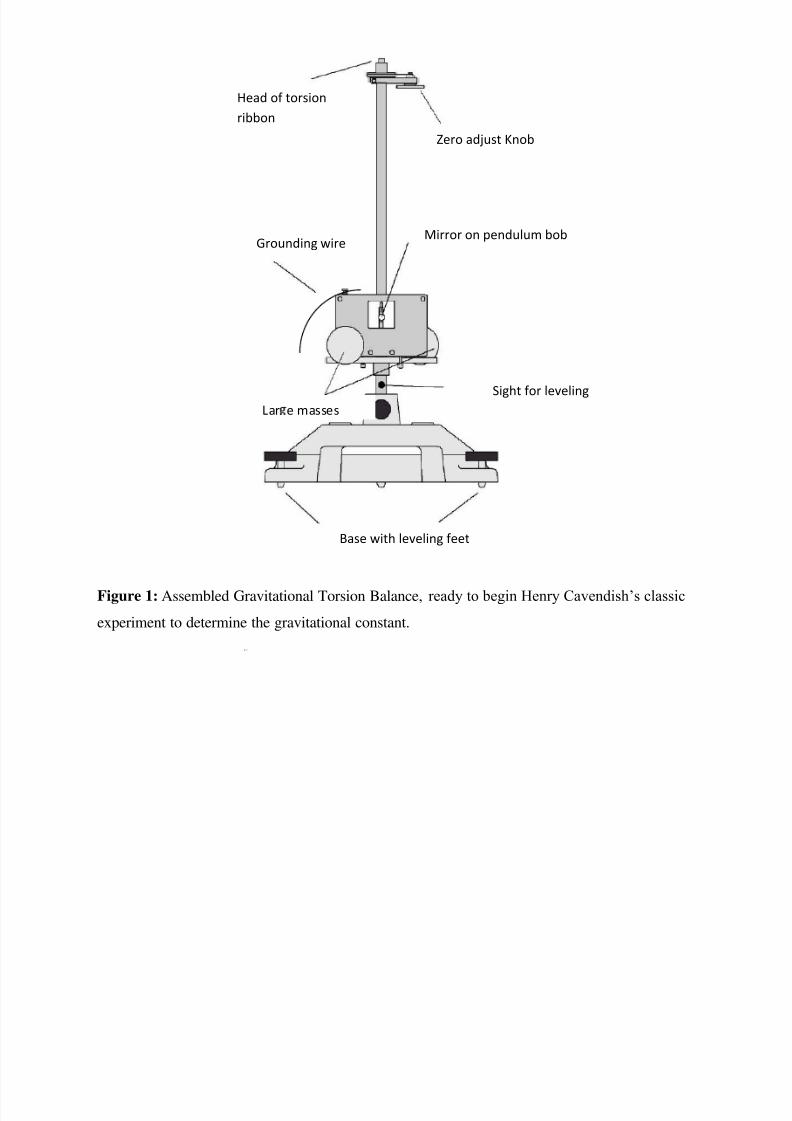
Figure 1: Assembled Gravitational Torsion Balance, ready to begin Henry Cavendish‘s classic

experiment to determine the gravitational constant.

Zero adjust Knob

Head of torsion

ribbon

Grounding wireMirror on pendulum bob

Sight for levelingLar e masses

Base with leveling feet

7/30/2019 Phy315 Manual 2


Equipment:

Included:

- Gravitational Torsion Balance

- Support base with leveling feet

- 1.5 kg lead ball (2)

- Plastic plate - Replacement torsion ribbon (part no. 004-06788)

- 2-56 x 1/8 Phillips head screws (4)

- Phillips screwdriver (not shown)

Additional Required:

• laser light source (such as the PASCO OS-9171 He-Ne Laser)

• meter stick

Torsion ribbon head

Zero adjust 1.5 kg lead

Knob masses

Figure -2: Equipment includes.

Replacement torsion

ribbon

2-56x1/8 Phillips

head screws

Plastic demons.

Leveling feet

Largemass

Swivel support

Al. Plate

Pendulum

mirror

Optical grade glass

window

Leveling sight

7/30/2019 Phy315 Manual 2


Equipment Parameters

• Small lead balls

Mass: 38.3 g + 0.2 g (m2) Radius: 9.53 mm

Distance from ball center to torsion axis: d = 50 .0 mm

• Large lead balls

Mass: 1500 g + 10 g (m1) Radius: 31.9 mm

• Distance from the center of mass of the large ball to the center of mass of the small ball when the

large ball is against the aluminum plate and the small ball is in the center position within the case: b =

46.5 mm (Tolerances will vary depending on the accuracy of the horizontal alignment of the

pendulum.)

• Distance from the surface of the mirror to the outer surface of the glass window: 11.4 mm

• Torsion Ribbon Material: Beryllium Copper

Length: approx. 260 mm

Cross-section: .017 x .150 mm

Important Notes:

The Gravitational Torsion Balance is a delicate instrument. We recommend that you set it up in a

relatively secure area where it is safe from accidents and from those who don‘t fully appreciate delicate

instruments.

The first time you set up the torsion balance, do so in a place where you can leave it for at least one

day before attempting measurements, allowing time for the slight elongation of the torsion band that

will occur initially.

Keep the pendulum bob secured in the locking mechanisms at all times, except while setting up and

conducting experiments.

Equipment Setup

Initial Setup

1. Place the support base on a flat, stable table that is located such that the Gravitational Torsion

Balance will be at least 5 meters away from a wall or screen.

Note: For best results, use a very sturdy table, such as an optics table.

2. Carefully remove the Gravitational Torsion Balance from the box, and secure it in the base.

3. Remove the front plate by removing the thumbscrews (Figure 3), and carefully remove the packing

foam from the pendulum chamber.

7/30/2019 Phy315 Manual 2


Note: Save the packing foam, and reinstall it each time the Gravitational Torsion Balance is

transported.

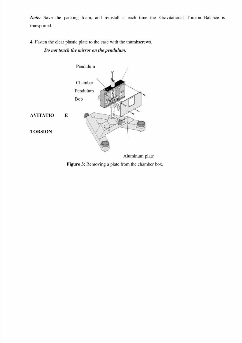
4. Fasten the clear plastic plate to the case with the thumbscrews.

Do not touch the mirror on the pendulum.

Pendulum

Chamber

Pendulum

Bob

AVITATIO E

TORSION

Aluminum plate

Figure 3: Removing a plate from the chamber box.

7/30/2019 Phy315 Manual 2


Leveling the Gravitational; Torsion Balance

1. Release the pendulum from the locking mechanism by unscrewing the locking screws on the case.

Lowering the locking mechanisms to their lowest positions (fig.4).

Figure-4: Lowering the locking mechanism to release the pendulum bob arms.

2. Adjust the feet of the base until the pendulum is centered in the leveling sight (figure -5). (The base of

the pendulum will appear as a dark circle surrounded by a ring of light).

3. Orient the Gravitational Torsion Balance so the mirror on the pendulum bob faces a screen or wall that

is at least 5 meters away.

Vertical Adjustment of the Pendulum

The base of the pendulum should be flush with the floor of the pendulum chamber. If it is not, adjust

the height of the pendulum:

1. Grasp the torsion ribbon head and loosen the Phillips retaining screw (Figure 6a).

2. Adjust the height of the pendulum by moving the torsion ribbon head up or down so the base of the

pendulum is flush with the floor of the pendulum chamber

(Figure 6b).

3. Tighten the retaining (Phillips head) screw.

7/30/2019 Phy315 Manual 2


Figure -5: Using the leveling sight to level the Gravitational Torsion Balance.

Torsion ribbon head

Torsion

ribbon

Pendulum

Pendulum bob must be centered

over the mirrorLook through the sight to view the reflection of the pendulum bob in the mirror.

mirror

7/30/2019 Phy315 Manual 2


Note: Vertical adjustment is only necessary at initial setup and when you change the torsion ribbon or

if someone has loosened the retaining screw by mistake; it is not normally done during each

experimental setup.

Rotational Alignment of the Pendulum Bob Arms (Zeroing)

The pendulum bob arms must be centered rotationally in the case

— That is, equidistant from each side of the case (Figure 7). To adjust them:

1. Mount a metric scale on the wall or other projection surface that is at least 5 meters away from the

mirror of the pendulum.

2.

Replace the plastic cover with the aluminum cover. 3. Set up the laser so it will reflect from the mirror to the projection surface where you will take your

measurements (approximately 5 meters from the mirror). You will need to point the laser so that it is

tilted upward toward the mirror and so the reflected beam projects onto the projection surface (Figure

8). There will also be a fainter beam projected off the surface of the glass window.

4. Rotationally align the case by rotating it until the laser beam projected from the glass window is

centered on the metric scale (Figure 9).

5. Rotationally align the pendulum arm:

a. Raise the locking mechanisms by turning the locking screws until both of the locking mechanisms

barely touch the pendulum arm. Maintain this position for a few moments until the oscillating energy of

the pendulum is dampened.

b. Carefully lower the locking mechanisms slightly so the pendulum can swing freely. If necessary, repeat

the dampening exercise to calm any wild oscillations of the pendulum bob.

c. Observe the laser beam reflected from the mirror. In the optimally aligned system, the equilibrium point

of the oscillations of the beam reflected from the mirror will be vertically aligned below the beam

reflected from the glass surface of the case (Figure 9).

7/30/2019 Phy315 Manual 2


d. If the spots on the projection surface (the laser beam reflections) are not aligned vertically, loosen the

zero adjust thumbscrew, turn the zero adjust knob slightly to refine the rotational alignment of the

pendulum bob arms (Figure 10), and wait until the movement of the pendulum stops or nearly stops.

e. Repeat steps 4a – 4c as necessary until the spots are aligned vertically on the projection surface.

6.

When the rotational alignment is complete, carefully tighten the zero adjust thumbscrew, being carefulto avoid jarring the system.

7/30/2019 Phy315 Manual 2


Hints for speedier rotational alignments:

• Dampen any wild oscillations of the pendulum bob with the locking mechanisms, as described;

• Adjust the rotational alignment of the pendulum bob using small, smooth adjustments of the zero adjust

knob;

• Exercise patience and finesse in your movements

7/30/2019 Phy315 Manual 2


7/30/2019 Phy315 Manual 2


Measuring the Gravitational Constant

Over View of the Experiment

The gravitational attraction between a 15 gram mass and a 1.5 kg mass when their centers are

separated by a distance of approximately 46.5 mm (a situation similar to that of the Gravitational

Torsion Balance ) is about 7 x 10 -10 Newton‘s. If this doesn‘t seem like a small quantity to measure,

consider that the weight of the small mass is more than two hundred million times this amount.

The enormous strength of the Earth's attraction for the small masses, in comparison with their attraction

for the large masses, is what originally made the measurement of the gravitational constant such a

difficult task. The torsion balance (invented by Charles Coulomb) provides a means of negating the

otherwise overwhelming effects of the Earth's attraction in this experiment. It also provides a force

delicate enough to counterbalance the tiny gravitational force that exists between the large and small

masses. This force is provided by twisting a very thin beryllium copper ribbon.

The large masses are first arranged in Position I, as shown in Figure 12, and the balance is

allowed to come to equilibrium. The swivel support that holds the large masses is then rotated, so the

large masses are moved to Position II, forcing the system into disequilibrium. The resulting oscillatory

rotation of the system is then observed by watching the movement of the light spot on the scale, as the

light beam is deflected by the mirror.

Any of three methods can be used to determine the gravitational constant, G, from the motion of the

small masses. In Method I, the final deflection method, the motion is allowed to come to resting

equilibrium — a process that requires several hours — and the result is accurate to within approximately

5%. In method II, the equilibrium method, the experiment takes 90 minutes or more and produces an

accuracy of approximately 5% when graphical analysis is used in the procedure. In Method III, the

acceleration method, the motion is observed for only 5 minutes, and the result is accurate to within

approximately 15%.

Note1: 5% accuracy is possible in Method I if the experiment is set up on a sturdy table in an isolated

location where it will not be disturbed by vibration or air movement.

Note2: 5% accuracy is possible in Method II if the resting equilibrium points are determined using a

graphical analysis program.

7/30/2019 Phy315 Manual 2


METHOD I: Measurement by Final Deflection

Setup Time – 45 minutes; Experiment Time: several hours

Accuracy: 5 %

Theory

With the large masses in Position I (Figure 13), the gravitational attraction, F between each small

(m) and is neighboring large mass (m1) is given by the law of universal gravitation:

F= G m1 m2 /b2 (1.1)

Where b= the distance between the centers of the two masses.

The gravitational attraction between the two small masses and their neighboring large masses

produces a net torque (τgrav) on the system

τgrav = 2Fd (1.2)

Since the system is in equilibrium, the twisted torsion band must be supplying an equal and

opposite torque. This torque(τband) is equal to the torsion constant for the band (k) times the

angle through which it is twisted (θ), or

τband = -kθ (1.3)

7/30/2019 Phy315 Manual 2


Combining equations 1.1, 1.2, and 1.3, and taking into account that τgrav = – τband, gives:

kθ = 2dGm1m2 / b2

Rearranging this equation gives an expression for G: (1.4)

To determine the values of k and θ — the only unknowns in equation 1.4 — it is necessary to

observe the oscillations of the small mass system when the equilibrium is disturbed. To disturb

the equilibrium (from S1), the swivel support is rotated so the large masses are moved to Position

II. The system will then oscillate until it finally slows down and comes to rest at a new

equilibrium position (S2) (Figure 14).

At the new equilibrium position S 2, the torsion wire will still be twisted through an angle θ , but

in the opposite direction of its twist in Position I, so the total change in angle is equal to 2 θ .

Taking into account that the angle is also doubled upon reflection from the mirror (Figure 15):

ΔS = S2 – S1,

4θ = ΔS/L or

θ= ΔS/4L (1.5)

7/30/2019 Phy315 Manual 2


The torsion constant can be determined by observing the period (T ) of the oscillations, and then

using the equation:

(1.6)

Where, I is the moment of inertia of the small mass system.

7/30/2019 Phy315 Manual 2


7/30/2019 Phy315 Manual 2


the force of attraction to the nearest large mass only.

Similarly,

Where G is your experimentally determined value for the gravitational constant, and G0 is

corrected to account for the systematic error.

Finally,

Use this equation with equation 1.9 to adjust your measured values.

METHOD II: Measurement by Equilibrium Positions

Observation Time: ~ 90+ minutes

Accuracy: ~ 5 %

Theory:

When the large masses are placed on the swivel support and moved to either Position I or

Position II, the torsion balance oscillates for a time before coming to rest at a new equilibrium

position. This oscillation can be described by a damped sine wave with an offset, where the value

of the offset represents the equilibrium point for the balance. By finding the equilibrium point for

both Position I and Position II and taking the difference, the value of S can be obtained. The

remainder of the theory is identical to that described in method I.

Procedure

1. Set up the experiment following steps 1 – 3 of Method I.

2. Immediately after rotating the swivel support to Position II, observe the light spot. Record the

position of the light spot (S ) and the time (t ) every 15 seconds. Continue recording the position

and time for about 45 minutes.

3. Rotate the swivel support to Position I. Repeat the procedure described in step 2.

Note: Although it is not imperative that step 3 be performed immediately after step 2, it is a good

idea to proceed with it as soon as possible in order to minimize the risk that the system will be

disturbed between the two measurements. Waiting more than a day to perform step 3 is not

advised.

Analysis

1. Construct a graph of light spot position versus time for both Position I and Position II. You will

7/30/2019 Phy315 Manual 2


now have a graph similar to Figure 18.

2. Find the equilibrium point for each configuration by analyzing the corresponding graphs using

graphical analysis to extrapolate the resting equilibrium points S1 and S2 (the equilibrium point

will be the center line about which the oscillation occurs). Find the difference between the two

equilibrium positions and record the result as ΔS.

3. Determine the period of the oscillations of the small mass system by analyzing the two

graphs. Each graph will produce a slightly different result. Average these results and record the

answer as T.

4. Use your results and equation 1.9 to determine the value of G.

5. The value calculated in step 4 is subject to the same systematic error as described in Method I.

Perform the correction procedure described in that section ( Analysis, step 3) to find the value of

G0.

Note: To obtain an accuracy of 5% with this method, it is important to use graphical analysis of

the position and time data to extrapolate the resting equilibrium positions, S1 and S2.

METHOD III:

Measurement by Acceleration

Observation Time: ~ 5 minutes

Accuracy: ~ 15%

7/30/2019 Phy315 Manual 2


Theory

With the large masses in Position I, the gravitational attraction, F , between each small mass (m2)

and its neighboring large mass (m1) is given by the law of universal gravitation:

F = Gm1m2 /b2 (3.1)

This force is balanced by a torque from the twisted torsion ribbon, so that the system is in

equilibrium. The angle of twist, θ is measured by noting the position of the light spot where the

reflected beam strikes the scale. This position is carefully noted, and then the large masses are

moved to Position II. The position change of the large masses disturbs the equilibrium of the

system, which will now oscillate until friction slows it down to a new equilibrium position.

Since the period of oscillation of the small masses is long (approximately 10 minutes), they do

not move significantly when the large masses are first moved from Position I to Position II.

Because of the symmetry of the setup, the large masses exert the same gravitational force on the

small masses as they did in Position I, but now in the opposite direction. Since the equilibrating

force from the torsion band has not changed, the total force (F total ) that is now acting to

accelerate the small masses is equal to twice the original gravitational force from the large

masses, or:

F total

= 2F = 2Gm1m

2/b

2 (3.2)

Each small mass is therefore accelerated toward its neighboring large mass, with an initial

acceleration (a0) that is expressed in the equation:

m2a0 = 2Gm1 m2 /b2 (3.3)

Of course, as the small masses begin to move, the torsion ribbon becomes more and more

relaxed so that the force decreases and their acceleration is reduced. If the system is observed

over a relatively long period of time, as in Method I, it will be seen to oscillate. If, however, the

acceleration of the small masses can be measured before the torque from the torsion ribbon

changes appreciably, equation 3.3 can be used to determine G. Given the nature of the motion —

damped harmonic — the initial acceleration is constant to within about 5% in the first one tenth of

an oscillation. Reasonably good results can therefore be obtained if the acceleration is measured

in the first minute after rearranging the large masses, and the following relationship is used:

G = b2a0 / 2m1 (3.4)

7/30/2019 Phy315 Manual 2


The acceleration is measured by observing the displacement of the light spot on the screen. If, as

is shown in Figure 19:

Δs = the linear displacement of the small masses,

d = the distance from the center of mass of the small masses to the axis of rotation of the torsion

balance,

ΔS = the displacement of the light spot on the screen, and

L = the distance of the scale from the mirror of the balance,

Then, taking into account the doubling of the angle on reflection,

ΔS = Δs(2L/d ) (3.5)

Using the equation of motion for an object with a constant acceleration ( x = 1/2 at 2), the

acceleration can be calculated:

a0 = 2Δs/t 2 = ΔSd/t

2 L (3.6)

7/30/2019 Phy315 Manual 2


7/30/2019 Phy315 Manual 2


References:

1. M.H.Shamos, Great Experiments in Physics, (Henry Holt & Co. New York 1959) p. 75, contains

Cavendish‘s original paper.

2.

B.E. Clotfelter, The Cavendish experiment as Cavendish knew it, Am. J. Phys 55, 210, 1987.3. J.Cl. Dousse and C. Rheme, A Student Experiment for Accurate Measurements of the Newtonian

Gravitational Constant, Am. J. Phys 55, 706, 1987.

4. Y.T. Chen and A. Cook, Gravitational Experiments in the Laboratory, (Cambridge University

Press, 1993).

7/30/2019 Phy315 Manual 2


The Franck – Hertz Experiment

Objective:

Electrons are accelerated in a glass tube filled with mercury vapour. Depending on the

acceleration voltage, a variable electron flux passes through the mercury vapor to the collector

electrode.

Equipments: COBRA3 Basic Unit(1), Power Supply, 12 V_(1),RS232 Data cable(1),Cobra3

Universal Plotter Software(1),Franck-Hertz Oven(1),Power supply unit for F.-H. tube(1),Power

supply, 0…600V-(1),DC measuring amplifier(1),Digital Thermometer(1),Ni Cr-Ni

thermocouple(1), BNC cable(2), Short – circuit plug(1),Plate, ceramic fiber(1),Connecting

cords(12).

Set- up:

- In accordance with Figs. 1 and 2.

- The power supply for the Franck – Hertz tube is required to generate a 0 to -50 V rising voltage

from a constant supply voltage (50V-). As long as the switch S (short – circuit plug) is closed, the

anode voltage is approximately 0.5 V. After the switch has been opened, the voltage increasedlogarithmically.

- Over a voltage divider (2x100 kΩ) that is integrated in the control unit , the voltage across thecathode and the grid UA is divided in a ratio of 1:2(i.e.UA /2) so that it can be measured by the

Cobra3 interface( Measuring range Analog IN2). Subsequent to the measurement, the

divided voltage is multiplied by two to obtain the true voltage across the cathode and grid.

- Over the voltage divider that is also integrated in the control unit, the 0……12V voltage is splitdown in order to be able to apply it as counter voltage to the collector electrode on the Franck – Hertz tube. When U=12 V, the split down voltage Us=3 V. The counter voltage can thus be

regulated in the region from 0 to 3 V. Us=0.5V should be applied at the beginning of the

experiment.

- The electron current that is conducted through the tube is on the order of 10-9

A. It is amplified by

the DC measuring amplifier (10 nA…. 10 A measuring range) and feed to the Analog IN 1

Channel on the Cobra3 unit.

- Heat the oven up to approximately 1600C. The tip of the temperature sensor is located at an

intermediate tube height, exposed to the air. After approximately 10 to 15 min, the apparatus is

ready for measurements.

Procedure:

- Start the ―Universal Plotter‖ and set the parameters according to Fig.3.

- When the < Continue> icon has been clicked up on, two digital displays, which show the currentvoltage without permanently recording the values, become visible. Using the set knob on the DC

measuring amplifier, set the voltage measured on the Analog channel with the switch S (short

circuit switch) closed to approximately 0 V.

7/30/2019 Phy315 Manual 2


- Then click on the ―Start measurement‖ icon and open switch S (Pull the short circuit plug).Itnow takes approximately 1.5 minutes to complete the measurement. Finally, the digital panel for

Analog channel IN2 indicates approximately 25 V. Now, approximately 50 V lie across the

cathode and the grid. Click on the < Stop Measurement> icon.

Fig.1: Experimental setup.

Fig.2: Circuit diagram for the Franck-Hertz experiment.

7/30/2019 Phy315 Manual 2


Caution:

- During the measurement processes watch the tube! If a bright bluish light suddenly appears

between the cathode and the grid, the tube has ―ignited‖. Shut switch S immediately (Plug in the

short circuit switch!)to eliminate the intense light , which can damage the cathode . If this occurs,

increase the oven temperature and restart the measurement.

Fig .3: Measurement Parameters.

A weak greenish light that is arranged in horizontal layers is harmless: it shows the shock fronts

of the electrons with the mercury atoms.

- Convert the Analog channel IN 2 in the Analysis / Channel modification window, using the

formula x: = x*2, into the true voltage that lay across the cathode and the grid during the

measurement. (The voltage splitter ratio of 1:2 is mathematically reversed!).

- Change the unit of the Analog channel IN 1 into current in Measurement / Information …/Channels window: Symbol, I; Unit, nA.

- In the Measurement / Channel Manager window, select the following: for the x axis, Analog

channel IN 2: and for the y axis, the current channel (Fig.5).

7/30/2019 Phy315 Manual 2


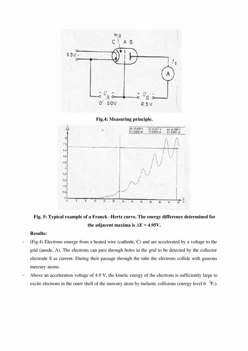
Fig.4: Measuring principle.

Fig. 5: Typical example of a Franck – Hertz curve. The energy difference determined for

the adjacent maxima is ∆E = 4.95V.

Results:

- (Fig.4) Electrons emerge from a heated wire (cathode, C) and are accelerated by a voltage to the

grid (anode, A). The electrons can pass through holes in the grid to be detected by the collector

electrode S as current. During their passage through the tube the electrons collide with gaseous

mercury atoms.

- Above an acceleration voltage of 4.9 V, the kinetic energy of the electrons is sufficiently large to

excite electrons in the outer shell of the mercury atom by inelastic collisions (energy level 63P1).

7/30/2019 Phy315 Manual 2


7/30/2019 Phy315 Manual 2


C= 2.9979 x 108

m/s , h = 4.136 x 10-15

eV,

It lies in the UV region.

Remarks:

- In general the following are true:

- The low energy maxima and minima can be better observed at low tube temperatures. However,

the tube ignites extremely easily under these conditions. The Higher – energy maxima and

minima can be better observed at high temperatures. At high temperatures the energy difference

between a minimum and its adjacent maximum becomes continuously smaller.

- If the oven continues to heat up during the recording of the measure values, the high – energy

peaks on the curve can easily migrate downward. However , for the evaluation this effect is

inconsequential as only the voltage differences of the peaks are measured and not their

amplitudes.

- If an older power supply that has no output jack for UA /2 is used for the Franck – Hertz tube ; the

following equipment is required:

- Switch box(1),Resistor in plug – in box , 100 k Ω(2),Connection cord(2)

References:

- G. Rapior, K. Sengstock and V. Baeva, ―New Features of Franck -Hertz Experiment‖. Am. J.

Phys. 74(5), 423-28 (2006).

- J.S. Huebner, ―Comments on the Franck -Hertz Experiment. Am.J. Phys. 44,302-03(1976).- H. Haken and H.C. Wolf, The Physics of Atoms and Quanta,6 th Ed.

SpringerHeidelberg,P.305(2000).

7/30/2019 Phy315 Manual 2


NiCr- Ni

Table of operative temperatures, tolerances and EMF values in mV at different temperatures for

thermocouples NiCr- Ni DIN 43710

0C 0 10 20 30 40 50 60 70 80 90 100 mv/ 0C Toll.in0C

0 0 .40 0.80 1.20 1.61 2.02 2.43 2.85 3.2 3.68 4.10 0.041

100 4.10 4.51 4.92 5.33 5.73 6.13 6.53 6.93 7.33 7.73 8.13 0.040

200 8.13 8.54 8.94 9.34 9.75 10.16 10.57 10.98 11.39 11.80 12.21 0.041

300 12.21 12.63 13.04 13.46 13.88 14.29 14.71 15.13 15.55 15.98 16.40 0.042

400 16.40 16.82 17.24 17.67 18.09 18.51 18.94 19.36 19.79 20.22 20.65 0.042

500 20.65 21.07 21.50 21.92 22.35 22.78 23.20 23.63 24.06 24.49 24.91 0.043

600 24.91 25.34 25.76 26.19 26.61 27.03 27.45 27.87 28.29 28.72 29.14 0.042

700 29.14 29.56 29.97 30.39 30.81 31.23 31.65 32.06 32.48 32.89 33.30 0.042

800 33.30 33.71 34.12 34.53 34.93 35.34 35.75 36.15 36.55 36.96 37.36 0.041

900 37.36 37.76 38.16 38.56 38.95 39.35 39.75 40.14 40.53 40.92 41.31 0.040

1000 41.31 41.70 42.09 42.48 42.87 43.25 43.63 44.02 44.40 44.78 45.16 0.039

1100 45.16 45.54 45.92 46.29 46.67 47.04 47.41 47.78 48.15 48.52 48.89 0.037

1200 48.89 49.25 49.62 49.98 50.34 50.69 51.05 51.41 51.76 52.11 52.46 0.036

7/30/2019 Phy315 Manual 2


Chaos Experiment

Object: - To study chaos in the diode- R-L circuit.

Theory:

Chaos typically refers to unpredictability or disorder mathematically, chaos means an a periodic

deterministic behavior. Chaotic systems look random but actually they are deterministic systems,

governed by non-linear equations. Hence such systems are very sensitive to the initial condition.

All chaotic systems, exhibit self-similarity i.e. the chaotic behavior resembles itself at all scales.

The Logistic Map and Frequency Bifurcations:

We are used to the notion that physical systems are described by differential equations that can

be initial condition. This is not true in complex systems governed by non-linear equations. A

typical example is the flow of fluids. At low velocity one can identify individual ―streamlines‖

and predict their evolution. However, when a particular combination of velocity, viscosity, andboundary dimensions is reached, turbulence sets in and eddies and vortices are formed. The

motion becomes chaotic. Many chaotic systems exhibit self – similarity: that is when the flow

breaks into eddies break into smaller eddies and so on. Such scaling is universal; it is observed in

all chaotic systems.

A particularly simple case is that of systems that obey the logistic map introduced in connection

with population growth. Designate by X j the number of members of a group may be the

population on an island, the bacteria in a colony, etc. The index j labels a population on an

interval (such as a day or a year) or the successive ―generations‖ of the population. If the

reproduction rate in one generation is λ, then it would hold that (1)

However the population will also decrease due to deaths.In particular if the food supply on the

island is finite the death rate will be proportional to x2 j. Thus the evolution

1is governed by the

map

(2)

We use the term map, because given x j we can find x j+1 uniquely .Both λ and s are assumednonnegative. We see immediately that if λ>1 and s=0 the population will grow exponentially,while if λ<1 the population will tend to 0. The map of Eq. (2) can be rescaled by introducing

for all j.

Then y j obeys the logistic map

7/30/2019 Phy315 Manual 2


(3)

The above map has the interesting property that if the reproduction rate for one generation is

restricted in the range

0 < λ < 4,

Then y j remains bounded between

0< y j < 1.

We are interested in the fate of the group after many generations, namely in the value of y j as

j→. We find, as already stated, that:

If λ ≤ 1, as j → y j → 0 the population decays to 0.

If 1 < λ < 3, as j → y j → y → y* the population tends to a stable point y*, namely. (4)

With solutions

y*=0,

In this case the solution y* = 0 is unstable, because if y0 = ε

(ε infinitesimal) y will tend to (1- 1/λ).

When λ > 3, the system behaves in a very different manner. As soon as λ> 3 but λ< 3.4495….the population alternate between 2 stable values. When λ> 3.4495…. the population alternates between 4 stable values until λ > 3.54…., where it alternates between 8 stable values; for λ >3.56…. the population alternates between 16 stable values, and this continues at ever more

closely spaced intervals of λ. We say that there is a bifurcation2 at these specific values of λ.

These results can be easily checked with a pocket calculator or a simple program. Table 1 gives

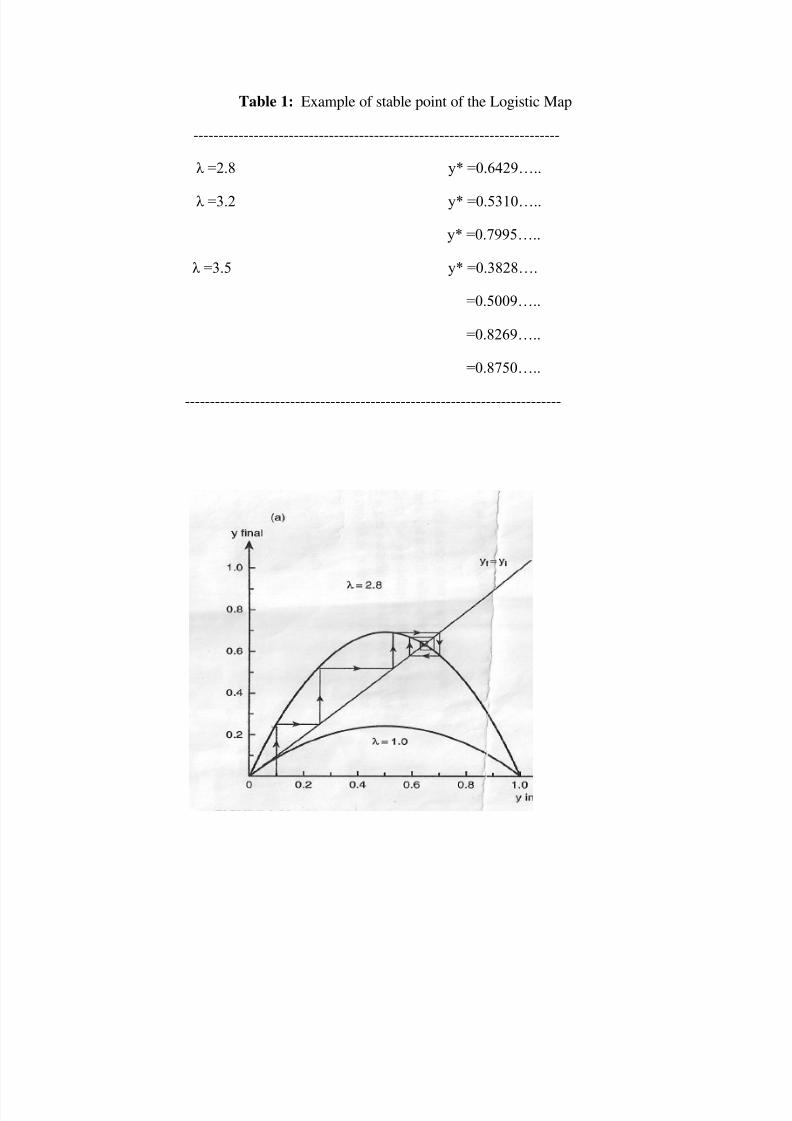
some typical result for λ = 2.8, λ =3.2, and λ =3.5, and the stable points are shown in thegraphical construction of Fig.1. What is plotted in Fig.1. is yfinal vs yinital. The continuous curve

is the equation of the logistic map yf = λ yi (1-yi). In Fig. 1a the cures

7/30/2019 Phy315 Manual 2


Table 1: Example of stable point of the Logistic Map

-------------------------------------------------------------------------

λ =2.8 y* =0.6429…..

λ =3.2 y* =0.5310…..

y* =0.7995…..

λ =3.5 y* =0.3828….

=0.5009…..

=0.8269…..

=0.8750…..

---------------------------------------------------------------------------

7/30/2019 Phy315 Manual 2


Figure1: Plot of the logistic map: for (a)λ=1.0, λ=2.8; λ=2.8 there is one stable point aty*=0.6429……..(b) for λ=3.2; there are two stable points at y*=0.7995….and y*=0.5130. seethe text for details of the path leading to the stable points.

For λ =2.8 and λ =1.0 are shown, while in Fig.1b the curve for λ =3.2.The lines for yf = yi are

also drawn. We can follow the path from some initial value y0 =0.1 in Fig.1a to the stable point

(indicated by a circle). Given yo we find y1 = yf at the intersection with the curve. However, y1must now be used as an input, yi, so we use the yf = yi line to locate yi and proceed to find y2 and

so on. The process converges to the circled point at y* = 0.6429…..

It is also evident that the same construction for the λ =1 curve will lead to y* = 0.0. In Fig.1b wenow find the two stable points at y* = 0.7995 and y* = 0.5130. The map requires that one stable

point leads to the next and vice versa.

When λ > 3.5699… the population no longer reaches a stable point but takes on an infinity of values in the range 0 < y <1. We say that the system behaves chaotically. This persists in the

remainder of the range 3.5699…. < λ < 4.0, but one finds regions of stability where an odd

number of stable points exist. The dependence of the bifurcations on λ is shown in Fig. 2. Wherethe λ – scale is highly nonlinear in order to shown enough detail; the vertical scale given values

y j* (j → ) of the stable point.

7/30/2019 Phy315 Manual 2


Fig.2. The stable points of the logistic map as a function of λ . The λ scale is highly nonline ar in

order to clearly show the bifurcations. The black parts of the plot indicate the chaotic region.

Note, however the thin white lines, which indicate islands of stability

The remarkable discovery by M. Feigenbaum in 1975 was that all systems that exhibits chaos

follow the same(universal) that the deference ∆n =λn+1 - λn of the values of the parameter at witch

bifurcations(period doubling) occur converges rapidly as n → . In particular as n→ the ratio,

(5)

is a universal constant.

Also, the amplitude at the stable point (while bifurcating) exhibits universal behavior. If yn (1)

and yn(2)are the two stable point of a given branch at the bifurcation value λn ,and

∆y*n =y*n(1)

– y*n(2)

Then,

lim ∆y*n / ∆yn+1 →α = 2.5029078…… (6)

n→

Here, δ and α are universal constant and are called Feigenbaum constant.

7/30/2019 Phy315 Manual 2


This indicates that as λ increases the system replicates itself after rescaling by a factor 1/α, asshown in Fig.2; typical intervals

3. ∆y*2 and ∆y*3 are indicated.

In this experiment, we study the chaotic behavior in a diode-R-L circuit, driven at its resonant

frequency. Here the diode is a non-linear device; hence bifurcation and chaos are natural for this

system. The effect was first reported by Linsay4

and was analyzed in details by Rollins andHunts

5. The circuit is shown below.

Fig.3: The diode-R-L CIRCUIT

Here, the source is assumed to be sinusoidal of amplitude V0 ,hence,

Va = V0 Cosωt

Then, for half the cycle, there is appositive voltage across the diode, during it conduct and

appears as an EMF.

√

Vb(t) = -Vf

During the other half, the diode dose not conduct draws a charging current, and the voltage at b

follows the frequency of the source. It can be calculated by

()

()

7/30/2019 Phy315 Manual 2


With √ –

and A, B, φ are constants.

The behavior of current and voltage are shown in Fig.4.

Clearly, the amplitude of Vb will change with every cycle.

Then depending on λ=V0 /VF, Vb repeats with a period T0,2T0,4T0 and so on fill it becomes

chaotic.

Observation:

To perform the experiment you should use a 1N 40007 diode , a inductance L=……..mH and a

resistance R=…………….Ω ,The source frequency F=………..kHz.

As you increase the V0 slowly, you can observe the bifurcation (in Vb) by an oscilloscope. The

Y-t and the X-Y traces of the bifurcations should be attach and the data obtained is given as

following.

Bifurcation V0(in V) Vb(inV) λn

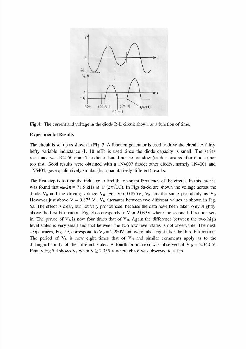
7/30/2019 Phy315 Manual 2


Fig.4: The current and voltage in the diode R-L circuit shown as a function of time.

Experimental Results

The circuit is set up as shown in Fig. 3. A function generator is used to drive the circuit. A fairly

hefty variable inductance (L=10 mH) is used since the diode capacity is small. The series

resistance was R 50 ohm. The diode should not be too slow (such as are rectifier diodes) nor

too fast. Good results were obtained with a 1N4007 diode; other diodes, namely 1N4001 and

1N5404, gave qualitatively similar (but quantitatively different) results.

The first step is to tune the inductor to find the resonant frequency of the circuit. In this case it

was found that ω0/2π = 71.5 kHz 1/ (2π√LC). In Figs.5a-5d are shown the voltage across the

diode Vb and the driving voltage V0. For V0< 0.875V, Vb has the same periodicity as V0.

However just above V0= 0.875 V , Vb alternates between two different values as shown in Fig.

5a. The effect is clear, but not very pronounced, because the data have been taken only slightly

above the first bifurcation. Fig. 5b corresponds to V0= 2.033V where the second bifurcation sets

in. The period of Vb is now four times that of V0. Again the difference between the two high

level states is very small and that between the two low level states is not observable. The next

scope traces, Fig. 5c, correspond to V0 = 2.280V and were taken right after the third bifurcation.

The period of Vb is now eight times that of V0 and similar comments apply as to the

distinguishability of the different states. A fourth bifurcation was observed at V 0 = 2.340 V.Finally Fig.5 d shows Vb when V0≥ 2.355 V where chaos was observed to set in.

7/30/2019 Phy315 Manual 2


Fig. 5: Oscilloscope traces of the voltage, Vb, across the diode (upper trace ) and of the driving

voltage V0 ( lower trace ) . The driving frequency is 71.5 kHz. (a) Immediately after the firstbifurcation. Note that the upper trace is bimodal and has period 2 T0. (b) Immediately after the

second bifurcation. Note that the large peaks are bimodal; the period is 4 T0. (c) Immediately

after the third bifurcation; the period is now 8 T0. (d) Chaotic behavior.

A plot of the bifurcations obtained for this diode is shown in Fig.6. The error in determining the

exact bifurcation voltage6

is + 5mV. We summarize the results in Table 2.

Fig.6: Plot of Vb Vs V0 as measured for the 1N4007 diode . The bifurcations are clearly

observed. Some ∆Vb spacing‘s are also indicated. Chaos sets in at V0 = 2.355 V.

7/30/2019 Phy315 Manual 2


Table 2: Bifurcation Data from Measurements of Chaos

Bifurcation V0(mV)

1st 875

2n

2033

3r 2280

4t

2340

Chaos 2355

From these data we calculate the Feigenbaum number δ. We have

λ2- λ1 = 1158 ± 7 mV

λ3-λ2 = 247 ± 7mV

λ4- λ3 = 60 ±7mV

and therefore

δ (1) =λλλλ

λλλλ

These results are consistent with the asymptotic value given in eq. (5). Even though input from

only the first four bifurcations was used.

The determination of the second Feigenbaum number α is not possible with the present data. As pointed out previously, the intervals ∆yn* must be selected appropriately, but even then (see

Fig.6) the ratios of ∆yn* seem much larger than α . This is due in part to the fact that one has notreached the asymptotic regime of Eq. (6) and in part to discontinuous jumps in Vb at certain

values7

of V0 . However, it is evident from the data that the system replicates itself after each

bifurcation. Furthermore, the spacing between stable points in every branch decreases in

subsequent bifurcations by a multiplicative factor ; this factor seems to converge toward

feigenbaum‘s α. We also note that for the 1N4001 diode it was possible to observe islands of stability in the chaotic region.

7/30/2019 Phy315 Manual 2


Notes and References:

1The first study of these issues is due to the English sociologist T. R. Malthus (1766-1834)

2 Henri Poincare in 1900 had noticed such behavior in mechanical systems and named it the

―exchange of stability.‖

3The intervals ∆yn*must be chosen appropriately as is also evident from Fig.2.

4P.S. Linsay , Phys. Rev. Lett. 47, 1349(1981).

5R. W. Rollins and E.R. Hunt , Phys. Rev. Lett. 49 , 1295 (1982); R.W. Rollins and E. R. Hunt ,

Phys. Rev. A29, 3327 (1984).

6

A more precise determination of the voltage at which bifurcation occurs can be made when asignal analyzer (FFT) is available. In this case the onset of period doubling is evident from the

appearance of sub harmonics in the frequency spectrum.

7Some diodes show marked hysteresis associated with these discontinuities.

8N. B. Tufillaro, T. Abbott and J. Reilly, An Experimental Approach to Nonlinear

Dynamics and Chaos, Addison-Wesley, New York, 1992.

9M. Hasler, ―Electrical circuits with chaotic behaviour,‖ Proceedings of IEEE,

Vol. 75, No. 8, pp. 1009 – 1021, August 1987.

10S. Prentiss, The Complete Book of Oscilloscopes, McGraw Hill, New York, 1992.

11C. W. Wu and N. F. Rulko, ―Studying chaos via 1-d maps: a tutorial‖ IEEE

Trans. Circ. Syst. I, Vol. 40, No. 10, pp. 707 – 721, October 1993.

12M. J. Ogorzalek, Chaos and Complexity in Nonlinear Electronic Circuits, World

Scientific Series on Nonlinear Science, Vol. 22, 1997.

7/30/2019 Phy315 Manual 2


Characterization of Solar Cell

Objectives:

1. Find Io and n from Dark I-V.

2. Find Voc .Isc and FF from illuminated I-V.

3. Find the efficiency η of the solar cell.

Introduction:

Crystalline Si p-n Solar Cell:

A solar cell or a photovoltaic cell is a semiconductor device to convert light into electricity. The

cell consists of a p-n junction of a semiconductors material having a band gap E g. When the cell

is exposed to light, a photon with energy,

less than Eg makes no contribution to the cell

output. However a photon with energy, greater than Eg contributes an energy Eg to the cell

output and the excess over Eg is dissipated as heat.

Theory:

Dark current of a p-n junction is given by,

Where n is the ideality factor and varies from n=1 to n=2 . Is is the dark saturation current and V

is the applied voltage. Hence k is Boltzmann constant and T is the operating temperature of

junction. Ec

/

n /

Ec /

Ef- - - - - - - - - - - - - - - - - - - - - - - - - - - - - -- - - - - -Ef

Ev

/

/ p

Ev /

Fig-1: Band diagram of a p-n junction

7/30/2019 Phy315 Manual 2


When light of energy greater than or equal to Eg is shown on the cell, electron – hole pairs are

generated because of absorption of light. Due to the inbuilt field in the p-n junction the photo

generated electrons and holes get separated and contribute to the current output if the cell is short

circuited. Under open circuit condition a voltage is generated across the solar cell called the open

circuit voltage. The equivalent circuit of the solar cell and the band diagram of a p-n junction

under illumination are shown in fig.2.

\

(a)

(b)

Fig.2: (a) Equivalent circuit of a solar cell and (b) The diagram of a p-n junction under

illumination.

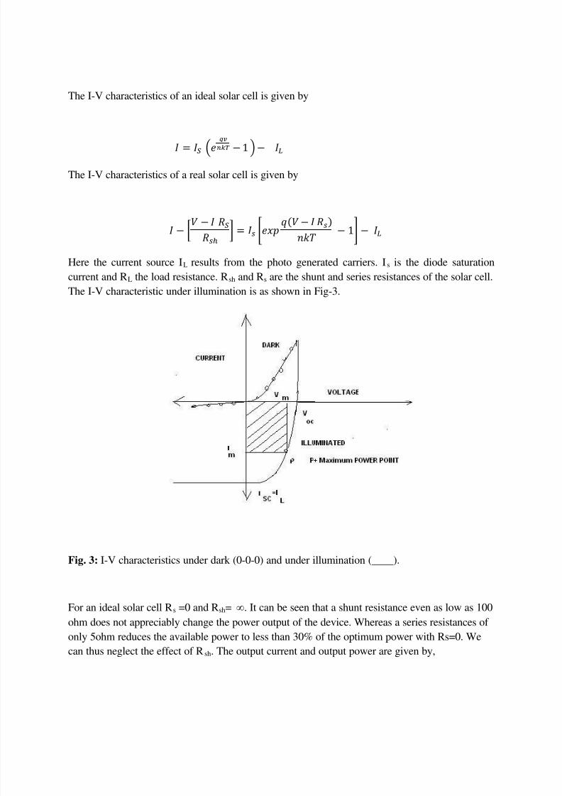
7/30/2019 Phy315 Manual 2


The I-V characteristics of an ideal solar cell is given by

The I-V characteristics of a real solar cell is given by

Here the current source IL results from the photo generated carriers. Is is the diode saturation

current and RL the load resistance. Rsh and Rs are the shunt and series resistances of the solar cell.The I-V characteristic under illumination is as shown in Fig-3.

Fig. 3: I-V characteristics under dark (0-0-0) and under illumination (____).

For an ideal solar cell Rs =0 and Rsh= . It can be seen that a shunt resistance even as low as 100

ohm does not appreciably change the power output of the device. Whereas a series resistances of

only 5ohm reduces the available power to less than 30% of the optimum power with Rs=0. We

can thus neglect the effect of Rsh. The output current and output power are given by,

7/30/2019 Phy315 Manual 2


7/30/2019 Phy315 Manual 2


Connect the circuit as shown in fig.4. Measure I-V characteristics under dark. Now connect the

circuit as shown in fig-4. Measure the intensity of the light, measure V oc and Isc. Take the I-V

characteristics by varying the resistance under illumination.

Referenence:

Physics of Semiconductor devices. SM Sze. IInd edition.

Thin Film Solar Cells: K.L. Chopra and S. R. Das

7/30/2019 Phy315 Manual 2


Rydberg Constant

Objective: Determination of Rydberg constant.

Apparatus: Hydrogen discharge tube together with induction coil, spectrometer, prism, grating

Introduction:

The energy levels of the hydrogen atom are obtain by solving the Schrodinger Equation; we get

(M.K.S.Unit) (1) The frequency v0 of emitted light is given by

(2)

Different transitions can be arranged into series known after their corresponding discovers

nf =1 , ni=2,3,4………… Lyman series (ultraviolet)

nf =2 , ni=3,4,5………… Balmer Series (Visible)nf =3 , ni-=4,5,6……….. Paschen Series (Infrared)

nf =4 , ni= 5,6,7……… Brackett Series (Infrad)

nf =5 , ni=6,7,8………. Pfund Series (Far infrared)

From Eq. (1) and (2) we get the inverse wavelength.

(3)

Rydberg constant R is defined as

(4)

So that its theoretical value is … ………… (5)

Procedure:

The object of the experiment is to determine R using Eq. (4). For Balmer series of lines .An

electric discharge tube is used to excite hydrogen atoms to higher levels and a gratingspectrometer is used to measure the wavelength of the emitted radiation.

Ensure the following standard adjustment in the spectrometer.

(1) The telescope is focused for infinity.

(2) The collimator is adjusted as to give a parallel beam.

(3) The turntable is leveled.(4) The turntable is so placed as to make the plane of the grating normal to the incident

beam.

(The last two adjustments are made by making sure that a particular image, say the red one infirst order, is observed at the same angle and the same height on the left and right sides).

7/30/2019 Phy315 Manual 2


Use a narrow slit and illuminate it by Hydrogen discharge tube and measure the angularPositions of diffraction images on both sides of the direct image .in all visible orders.

(You should be able to see at least three colors in the first and second orders. Try also to locate at

least one image in third order).Calculate the wavelength using the formula.

(6)

Where d is the spacing of the grating (grating has 15,000 lines /inch), m the order of diffraction,and ө is the angle of diffraction which is measured .Calculate R from Eq. 4 and compare it with

the theoretical value obtained from Eq. 5.

Note: To observe all diffraction images switch off all lights in the room.

References:1. B. L. Worsnop And N.T.Flint : Advanced Practical Physics for students ―(for

adjustment of the spectrometer).

2. D. D. Halliday and R. Resnick:‖Physics Part II (For grating ),P.1123-1134.3. A. Beiser:‘ Concepts of Modern Physics‘ (Ch.7) or R. B. Leighton :Principles of

Modern Physics (For theory of Hydrogen atom ).

7/30/2019 Phy315 Manual 2


7/30/2019 Phy315 Manual 2


7. With tape, mark the floor at regular intervals to about 10-20 meters from the laser. Allow for at

least 10 different intervals within the allotted space.

8. Using the BNC male – to-male cable, connect the TTL output of the function generator to

channel 1 of the oscilloscope.

9. Using the phone plug-to-BNC male cable, connect the power jack of the laser to the output of the

function generator.

10. Using the RCA male-to-BNC male cable, connect the ―video‖ output of the receiver to channel 2

of the oscilloscope.

11. Set the function generator for a square wave, and press the dc offset button. Turn the output and

DC offset knobs completely counterclockwise.

12. Turn the laser switch to the ―on‖ position.

13. On the function generator, turn up the DC offset knob until you see laser light. Do not look

directly into the laser light!

14. Align the laser, mirror, lens and receiver so that the laser is focused onto the ―video‖ sensing

element of the receiver.

15. Set the scope to dual trace:

a) Set channel 1 to 1v/div., DC.

b) Set channel 2 to1 v/div., AC.

c) Set the trigger to channel 1.

d) Set the trigger level to about 2.5 volts.

e) Set the time base to 50 ns/div.

16. Adjust the alignment of the laser, mirror, lens and receiver to maximize the sine wave signal on

channel 2

17. Adjust the DC offset and amplitude of the function generator to maximize the signal channel 2.

Diode laser- The diode laser emits an intense, narrowly-focused beam of light. In this

experiment, the diode laser is powered by a function generator, which modulates the light

intensity at approximately 3MHz. the laser is equipped with adjustment screws for precisely

aiming the light at the mirror.

Concave mirror-The concave surface of the mirror help to focus the light as it is reflected. The

mirror is also equipped with adjustment screws for aiming the light back to the receiver.

7/30/2019 Phy315 Manual 2


Light Receiver-The receiver is designed for receiving audio and video signal transmitted via

modulated light. Since the light receiver is sensitive to very high-frequency modulation, it is

ideally suited to the experiment, in this manual. There are two sensitive element on the receiver,

in this experiment, you will use only will use only the one labeled ―Video.‖

+127mm lens- the lens is used to focus the light onto the sensitive element of receiver.

Experiment 1: Modulated laser method for measuring the speed of light: In this experiment,

you will measure the speed of light using a laser modulated at a very high frequency and an

oscilloscope. You will measure the time, ∆t that elapses while the light signal travels a known

distance, ∆d, and you will calculate the speed of light, which is defined as ∆d/∆t.

The light signal, originating at the laser, will travel to mirror and back to the light receiver. You

will vary ∆d by moving the mirror and measuring the corresponding effect on ∆t with the

oscilloscope.t changes as ∆d varies.

Therefore, you will actually measure an elapsed time ∆t relative to an arbitrary (but constant)

baseline. This elapsed time can be expressed mathematically as: (1)

Where, tk is an unknown constant. For the same reason, you can also measure d‘ instead of ∆d

where

d (2)The equation of a line fitted to a plot of ∆d‘ vs. ∆t‘ (3)

Where, c represents the slope of the line. The combinations of equation 1, 2, and3 yields (4)

Where, K is another arbitrary constant. In equation 4, it is evident that the slope c, equals ∆d/∆t,

which is the speed of light.

Procedure:

1. Adjust the alignments of the laser and mirror and the positions of the lens and receiver to

maximize the signal. (Adjust the receiver up, down, left, and right on the carrier, but do not

change the position of the carrier on the bench.)

2. On the oscilloscope, adjust the scale and vertical position of the signal to maximize the signal

trace. Do not change the horizontal position of the trace.

7/30/2019 Phy315 Manual 2


3. Record the position of mirror (relative to its initial position) and the phase of the signal in Table

1. If your oscilloscope is equipped with cursors, use them to measure the phase. Otherwise,

estimate the phase to ½ of smallest division on the time scale.

4. Move the mirror back to the next mark and repeat steps 1 through 4.

Table 1

Mirror Position(m) Phase(s)

Analysis:

Plot ∆t vs. ∆d (Remember that ∆d is two times the mirror position. The slope of the best-fit line

is the speed of light.

Note: You can plot your data and obtain the best-fit line using Data Studio. For instructions, see

Appendix B of this manual.References:

1. A. A. Tyapkin, Lett. Nuovo Cimento, 7, 15, pp. 760-4, (1973).

2. H. Lorentz, Lectures on Theoretical Physics, V.1 pp. 14-19 (1927).

3. J. Larmor, Aether and Matter, Cambridge University Press (1900).

4. A. Michelson, E. Morley, Am. J. Sci, 34, 203, pp. 333 – 345 (1887).

5. M. Ruderfer, Phys. Rev. Lett. , 5, 5, pp.191-2 (1960).

6. K. Turner, H. Hill, Bull Am. Phys. Soc., 8, pp. 28 (1963).

7. D. Champeney, et. al., Phys. Lett., 7,4 ,pp.241-3 (1963).

8. M. Ruderfer, Phys. Rev. Lett. , 7, 9, pp. 361 (1961).

7/30/2019 Phy315 Manual 2


7/30/2019 Phy315 Manual 2


THIN FILM DEPOSITION WITH HHV UNIT

Operation Procedure:

1. Switch ON the power supply and ‗main MCB‘ of the system. Close all valves (Hivac-Valve

(HV) and Combination-Valve (CV) in closed position).

2. Close the chamber properly and switch on the Rotary pump.

3. Put CV to Roughing.

4. Wait till the vacuum reaches ~0.05 mbar in GH2.

5. Change CV to Backing.

6. Put water supply ON and switch ON the Diffusion Pump (DP).

7. Wait for around 20 mins, GH1 should show ~0.05 mbar now.

8. Change the CV to Roughing for 1-2 mins to get back ~0.05 mbar in GH2. Change the CV

back to Backing (~ 0.05 at GH1).

9. Put LN2 in the cold-trap.

10. Open the HV.

11. Wait for ~30 min. Expected vacuum is ~10-5

mbar.

12. Before deposition, attach the Digital Thickness Monitor (DTM) to the system.

13. For deposition select the particular source. Check that electrode‘s safety-shutter is closed.

Switch ON the LT. Be careful, high current flows through the system now-on.

14. Increase the current slowly at a rate of 2 Amp/Min. till deposition temp is reached.

15. Monitor the rate of deposition on the DTM (Preferably use shutter).

16. After deposition, decrease current at a rate of 2 Amp/Min.

17. After reaching back 0 Amp, wait 10 min and close the HV. Switch OFF the DP.

18. After ~20 mins, as the DP heater cools down, Put CV to Close, switch OFF the Rotary pump

and close water supply.

19. Deposition process is now complete. Vent the chamber to take the samples.

20. Leave the system back to vacuum using Rotary in Roughing mode.

7/30/2019 Phy315 Manual 2


Never do the Following:

1. Never put the CV on the Roughing when HV is Open (after step 10 above). This might spoil

the system permanently.

2. Never close the water supply when the DP is ON.

3. Never handle the valves roughly. Operate the valves slowly.

Special Reminders:

1. The system should not be operated in any case till you get the required permission.

2. Clean the chamber properly during uploading the substrates.

3. Always keep the system in vacuum. Remind yourself to keep it in vacuum before leaving the

lab.

3. Always close the water supply after all the processes.

4. Note the date, operation, task, sample positions, students actively present etc. in the Log-

Book. Any unusual incidence MUST be written down in detail in the Log-Book.

(I) Objective:

High Vacuum deposition and characterization of metallic thin film.

(II) Motivation:

Most scientists work with their samples in a vacuum system. The reasons for this are several

fold: first, many samples react with the gases in ordinary room air which means they must be

kept in a clean environment; second, the experimental probes used to measure sample properties

may depend on electron or other beams that simply could not exist outside a vacuum. Overall,

the quality of the thin film grown and the measurements done are of extremely high quality

under vacuum.

(III) The Instrument:

(IIIa) System Overview:

The system, illustrated in Figure 1, contains the essential elements typically required to obtain

high vacuum. The most common and reliable systems utilize three pumping devices: The

rotating mechanical pump, the diffusion pump, and the cold trap. Other system components, such

as valves and baffles, aid or control the action of these pumps. The rotary pump serves as a

primary source for creating vacuum. However, they can reach only upto ~ 10-3

mbar. The

Diffusion pumps using hot oil have the advantage of reaching ~ 10-7

mbar and has no moving

parts although they must be backed by a rotary pump. The cold trap reduces pressure by

7/30/2019 Phy315 Manual 2


condensing, or freezing out, onto its cold surfaces, condensable vapors that may exist in the

system. It also prevents oil vapor from the diffusion pump from diffusing back, or "back

streaming", into the system. By removing "condensables" such as water vapor, a trap actually

serves as a pump.

(IIIb) The Two Modes of Operation (Roughing and Backing):

Exposure to atmosphere when at operating temperature will result in decomposition of diffusion

pump oil. It is therefore necessary to employ a bypass line around a heated diffusion pump when

evacuating a chamber from atmospheric pressure to a "rough" vacuum prior to connecting the

chamber to the diffusion pump; hence, the terms "roughing line" and "roughing valve". The

foreline valve and the hi-vac valve (Figure 2) serve to isolate the diffusion pump, the baffle and

cold trap from the object being roughed. During roughing the roughing valve is open. When

roughing has been completed (at ~20 mtorr), the roughing valve is closed before the foreline

valve and the hi-vac valve are opened. The manifold vent valve admits air to the port manifold to

"break" the vacuum and make possible the removal of objects after they have undergone vacuum

Figure.1: The vacuum system illustrating the essential elements.

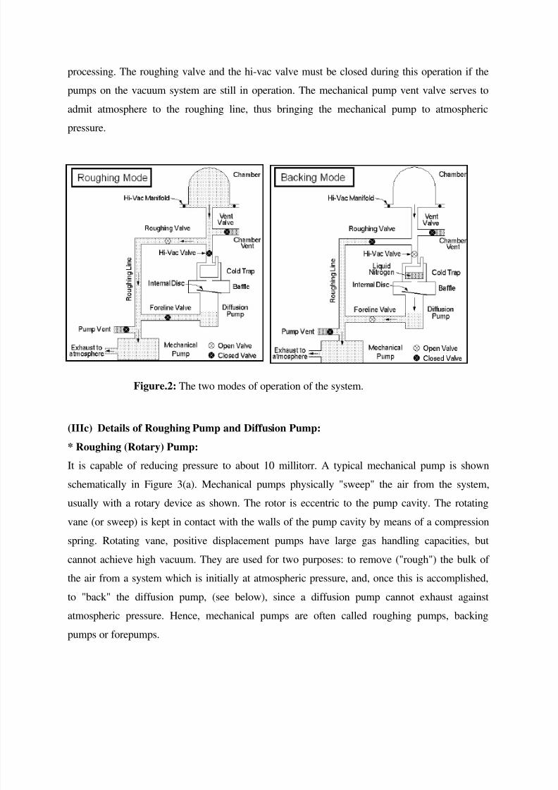
7/30/2019 Phy315 Manual 2


processing. The roughing valve and the hi-vac valve must be closed during this operation if the

pumps on the vacuum system are still in operation. The mechanical pump vent valve serves to

admit atmosphere to the roughing line, thus bringing the mechanical pump to atmospheric

pressure.

(IIIc) Details of Roughing Pump and Diffusion Pump:

* Roughing (Rotary) Pump:

It is capable of reducing pressure to about 10 millitorr. A typical mechanical pump is shown

schematically in Figure 3(a). Mechanical pumps physically "sweep" the air from the system,

usually with a rotary device as shown. The rotor is eccentric to the pump cavity. The rotating

vane (or sweep) is kept in contact with the walls of the pump cavity by means of a compression

spring. Rotating vane, positive displacement pumps have large gas handling capacities, but

cannot achieve high vacuum. They are used for two purposes: to remove ("rough") the bulk of

the air from a system which is initially at atmospheric pressure, and, once this is accomplished,

to "back" the diffusion pump, (see below), since a diffusion pump cannot exhaust against

atmospheric pressure. Hence, mechanical pumps are often called roughing pumps, backing

pumps or forepumps.

Figure.2: The two modes of operation of the system.

7/30/2019 Phy315 Manual 2


* Diffusion Pump:

It is capable of reducing system pressure to the region of 10-7 torr. A diffusion pump has a

maximum pressure against which it can exhaust; this is usually in the mtorr region. The

maximum exhaust pressure is also known as the "tolerable forepressure". The rotary pump noted

above provides and maintains this exhaust pressure for the diffusion pump. Fast pumping action

is achieved through the use of high speed jets of oil vapor which collide with gas molecules and

compress them in the direction of the mechanical pump (see Figure 3(b)). The term "jet" is used

to refer to both the vapor stream and to the nozzles from which the vapor issues. The oil pool at

the bottom of the pump is heated, causing oil vapor to be forced up the jet stack. The vapor

strikes the umbrellas, and is projected downward and outward through the nozzles of the jet

stack. In passing through the narrow jets, the oil vapor flows at a very high velocity (near that of

sound). The high speed vapor jet collides with gas molecules giving them a downward direction

toward the foreline. The oil molecules condense on the walls of the pump which are cooled

Figure.3. (a) the rotary vane pump and (b) the backing pump in action.

phy315 manual 2

Documents