phy862 – fall 2018 cryogenic systems
TRANSCRIPT

This material is based upon work supported by the U.S. Department of Energy Office of Science under Cooperative Agreement DE-SC0000661, the State of Michigan and Michigan State University. Michigan State University designs and establishes FRIB as a DOE Office of Science National User Facility in support of the mission of the Office of Nuclear Physics.
PHY862 – Fall 2018Cryogenic Systems
Pete Knudsen

Introduction
Processes that provide cooling to practical superconducting devices presently require cryogenic process conditions, namely temperatures generally below -150 ºC (~123 K)
Typically this involves working fluids that have a normal boiling point less than this temperature
Process cycles used to produce the required cooling are quite different from the more conventional vapor compression cycle
Week 1 | Slide 2
Introduction (cont.)
Key aspect to appreciate is the energy intensiveness •e.g., a typical large 4.5 K helium refrigerator requires three orders of magnitude more energy input (for the same cooling) than a normal home cooling system; a 2 K helium refrigerator requires three and often closer to four times what is required for 4.5 K refrigeration
In numbers: a typical large 4.5 K helium refrigerator requires ~250 W of input power per 1 W of cooling
A typical 2 K (~30 mbar) helium refrigerator requires ~1000 W/W, although it should be possible to achieve ~750 W/W for a well matched and well-designed system
Week 1 | Slide 3

So Why Superconductors & Why Helium?
Week 1 | Slide 4
Superconductor cables, implemented as electro-magnets, are commonly used in particle accelerators and colliders, MRI’s, plasma confinement (fusion research), and more
Practical type II superconductors (i.e., those made from alloys) used as electro-magnets, such as Nb-Ti and Nb3Sn, have transition temperatures of 9.6 K and 18.1 K, respectively
Transition temperatures correspond to zero current density at zero magnetic field, but some margin is needed for actual operation
•Note: The temperature, magnetic field and current (density) with which the superconductor transitions from normal to superconducting is a three-dimensional surface

Review of ThermodynamicsThermodynamic Laws – Describe what you cannot do in regards to work, heat, and temperature: •Zeroth Law: you cannot break any of the rules…even if you want to
•First Law: you cannot win – the best you can even dream about is breaking even
•Second Law: so much for your dream…because actually you cannot break even either...unless you somehow manage to reach absolute zero
•Third Law: the final dream crusher…you cannot reach absolute zero (temperature), unless you’re immortal
(Adapted from Wei Cai, Stanford Univ.)
Week | Slide 5

Review of Thermodynamics (cont.)
Week | Slide 6
Extensive properties – scale linearly with amount of substance(s) within the system; e.g., by ‘amount’ it is meant the mass ( ), number of moles ( ), or number of molecules•So, for example, the volume ( ), internal energy ( ), and entropy ( ) are extensive properties
Intensive properties – are independent of amount of substance(s) within the system•e.g., pressure ( ), temperature ( ), and electro-chemical potential ( )
If extensive properties like volume, internal energy, and entropy are scaled to the amount of substance(s) within the system (i.e., divide by the mass, moles, or molecules), then it becomes an intensive property•e.g., ⁄ , ̅ ⁄ , ⁄ , ⁄ , ⁄ , ̅ ⁄

Zeroth Law
Week | Slide 7
Zeroth Law – introduces temperature as an (intensive, macroscopic) state quantity, and defines thermodynamic equilibrium and is the basis of temperature measurement
•Thermal equilibrium – closed system who’s macroscopic state quantities are not changing with time
First Law
Week | Slide 8
Establishes the total energy as a state variable; also, called the “conservation of energy”To make sense of the First Law, the concept of (process) ‘path’ independence and conversely, (process) ‘path’ dependence must be established.Consider an equilibrium state ‘1’ and another (different) equilibrium state ‘2’ for a particular system; and (for simplicity) two different and arbitrary (process) ‘paths’ that we will call ‘a’ and ‘b’ Since the system energy is an (extensive) property, the change in energy is simply, ∆•i.e., it does not depend on the ‘path’, ‘a’ or ‘b’

First Law (cont.)
Week | Slide 9
For energy to be conserved, it must be true (according to the First Law) that the change in energy is equal to the work input and the heat input into the system; e.g.,
∆
Where, is the path dependent, or inexact differential, of the work into the system, and, is the path dependent, or inexact differential, of the heat into the system
That is, for path ‘a’ will not necessarily be equal for path ‘b’. Likewise for, In differential form, , noting that the energy is an exact, or path independent, differential

First Law (cont.)
Week | Slide 10
Work and heat are NOT state properties!
Note: some texts consider work positive if it leaves the system. The sign convention of work and heat is arbitrary, but its implementation must be consistent

Second Law
Week | Slide 11
Establishes entropy as a state variable describing the ‘quality’ or ‘availability’ of energyIf paths ‘a’ and ‘b’ are “reversible”, then we know experimentally that, ⁄•How would we empirically know this (an example)?...will come back to that (Clausius-Clapeyron equation)
Or, in integral form (Clausius equality),
∆
Where, is the (inexact) differential heat input from a “reversible” path

Second Law (cont.)
Week | Slide 12
As much as we can look at this as a definition of entropy as a state variable, we can also look at this as a definition of a reversible (process) path For a path ‘c’, between equilibrium states ‘1’ and ‘2’, which is notreversible,
∆
Which, referring back to the differential form, tells us that,
It should not escape one’s attention that in the First and Second Laws, inexact (path dependent) differentials yield exact (path independent) differentials; and visa-versa!

The Traditional Carnot Cycle
Week | Slide 13
The Carnot cycle can be a heat engine, transferring heat from a high temperature reservoir to a lower temperature reservoir with a net work output It can also be a refrigerator, operating in reverse and requiring a net work inputThe Carnot cycle does not convert heat energy!
s
Log(T0)
Log(T)
QL
QH
Wx Wc
CompressorExpander
Low Temperature Reservoir
High Temperature Reservoir
Wnet= Wc - Wx
ss
T=constantLog(T0)
Log(T)
QL
QHs =
con
stan
t
s = c
onst
ant
T=constant

The Carnot Cycle (cont.)
Week | Slide 14
So, from our discussion above, we know that,∆ ⁄ ⁄
And, from the First Law, we know that since we start and end at the same state point for a cycle,
∆ 0 ,
Where, , is the net work input; i.e., total input work ( ) minus total output work ( )
, ∆For an (isothermal) refrigerator, the coefficient of performance is defined as,
≡,
1

The Carnot Cycle (cont.)
Week | Slide 15
More commonly in cryogenics, we refer to the inverse of the coefficient of performance, as it is more representative of the energy intensiveness of such processes; i.e., ratio of net input work to cooling provided to the load
1
Note that to arrive at this result, we did not have to assume anything about the process between the reversible isothermal heat transfer steps, except that the entropy difference was constant at a given temperature
The ‘Generalized’ Carnot Cycle
Week | Slide 16
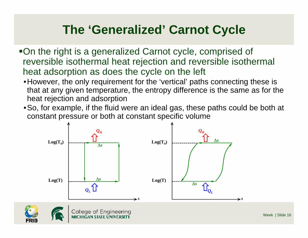
On the right is a generalized Carnot cycle, comprised of reversible isothermal heat rejection and reversible isothermal heat adsorption as does the cycle on the left •However, the only requirement for the ‘vertical’ paths connecting these is that at any given temperature, the entropy difference is the same as for the heat rejection and adsorption
•So, for example, if the fluid were an ideal gas, these paths could be both at constant pressure or both at constant specific volume
s
s
sLog(T0)
Log(T)
QL
QH
s
s
sLog(T0)
Log(T)
QL
QH

Third Law – Nernst’s Theorem
Week | Slide 17
As a system approaches absolute zero temperature, all processes cease and the entropy of the system approaches a minimum value (which can be defined as zero) It is not possible to reach absolute zero using any (physical) process, even if it were ideal Example: since constant pressure lines converge at zero temperature, it would take an infinite number of isentropic expansions with perfect counter-flow heat exchange to reach T=0 (Van Sciver, Helium Cryogenics, p. 15)

Third Law – Nernst’s Theorem (cont.)
Week | Slide 18
Coldest temperature ever recorded at ground level on Earth: 184 K (Soviet Vostok Station in Antarctica)Temperature of the moon (dark side), ~120 KDeep outer space background temperature: 2.7 KHe-3 / He-4 dilution refrigerator: ~1x10⁻³ K Adiabatic demagnetization using nuclear paramagnets: 1.5x10⁻⁶
K (lattice)MIT (2015): 4.5x10⁻¹⁰ K (Bose-Einstein condensate)
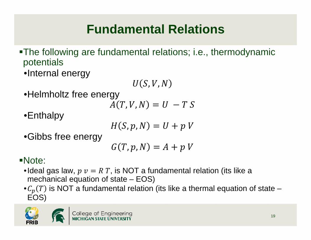
Fundamental RelationsThe following are fundamental relations; i.e., thermodynamic potentials•Internal energy
, ,•Helmholtz free energy
, , •Enthalpy
, , •Gibbs free energy
, , Note:
•Ideal gas law, , is NOT a fundamental relation (its like a mechanical equation of state – EOS)
• is NOT a fundamental relation (its like a thermal equation of state –EOS)
19

Derived Thermodynamic Properties
Week | Slide 20
Commonly encountered thermodynamic properties and their definitions:•Note: ⁄ , ⁄ , ⁄ , 1⁄ ; where, is the mass
Specific heat at constant pressure, ≡
Specific heat at constant volume, ≡
Volume expansivity, ≡
Isothermal compressibility, ≡
Joule-Thompson coefficient, ≡
Speed of sound (squared), ≡
Ratio of specific heats, ≡
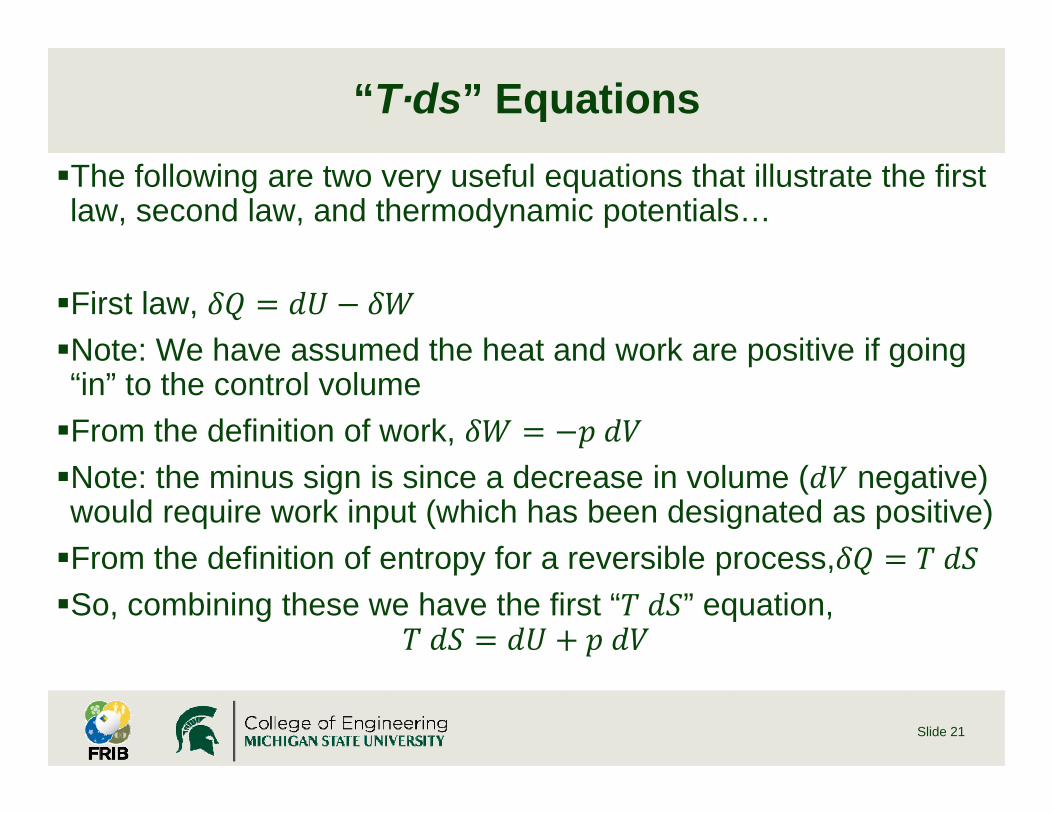
“T·ds” EquationsThe following are two very useful equations that illustrate the first law, second law, and thermodynamic potentials…
First law,Note: We have assumed the heat and work are positive if going “in” to the control volumeFrom the definition of work, Note: the minus sign is since a decrease in volume ( negative) would require work input (which has been designated as positive)From the definition of entropy for a reversible process, So, combining these we have the first “ ” equation,
Slide 21
“T·ds” Equations (cont.)
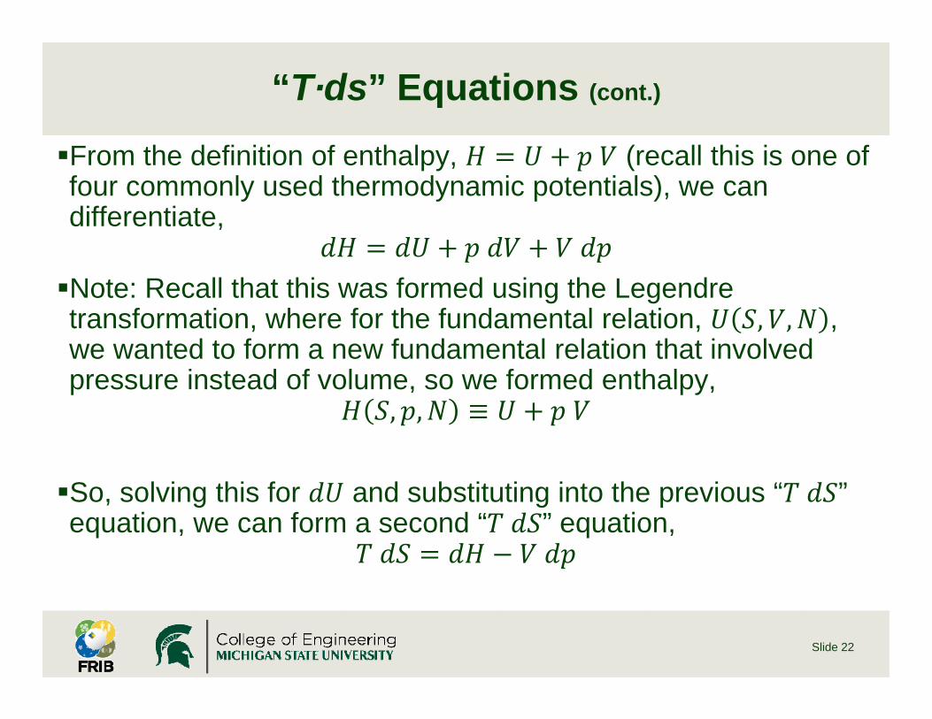
From the definition of enthalpy, (recall this is one of four commonly used thermodynamic potentials), we can differentiate,
Note: Recall that this was formed using the Legendre transformation, where for the fundamental relation, , , , we wanted to form a new fundamental relation that involved pressure instead of volume, so we formed enthalpy,
, , ≡
So, solving this for and substituting into the previous “ ” equation, we can form a second “ ” equation,
Slide 22
“T·ds” Equations (cont.)
Note: All of the variables in these two “ ” equations are state variables – they are not path dependent
Of course, for a fixed mass, we can divide by the mass and obtain the these equations such that all the state variables are intensive,
Slide 23

Reversible Work - ExergyFor a steady process (no mass or energy accumulation), the reversible work is,
Further, let us define the quantity of ‘physical exergy’,
≡ •Note that physical exergy has units of [J/kg]
So,
This equation, which is an extremely practical re-statement of the second law, is similar to the first law, with physical exergy (or just ‘exergy’) playing an analogous ‘role’ as the enthalpy; however, note that there is NO heat input/output
Slide 24

Reversible Work - Exergy (cont.)
Note: If there were another thermal reservoir at a temperature, say , there would be an additional term,
•Where,
•This is also known as the dimensionless energetic temperature and is the same as the Carnot efficiency (for the case where the environment temperature is the “low” temperature reservoir)
Exergetic efficiency is the ratio of the actual input power required ( ) to the reversible input power; i.e.,
⁄
Slide 25
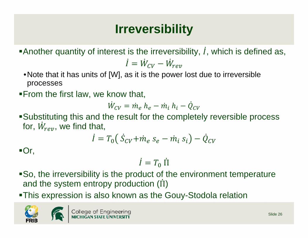
IrreversibilityAnother quantity of interest is the irreversibility, , which is defined as,
•Note that it has units of [W], as it is the power lost due to irreversible processes
From the first law, we know that,
Substituting this and the result for the completely reversible process for, , we find that,
Or,
ΠSo, the irreversibility is the product of the environment temperature and the system entropy production (Π)This expression is also known as the Gouy-Stodola relation
Slide 26
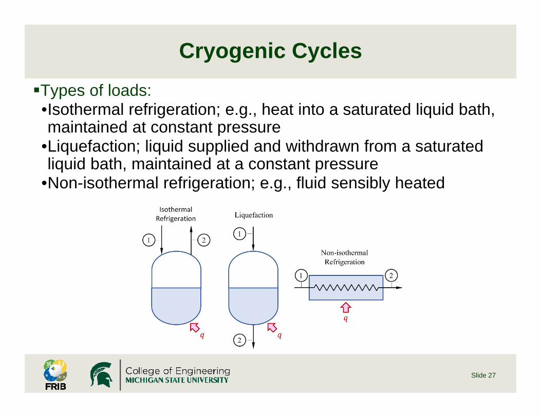
Cryogenic CyclesTypes of loads:•Isothermal refrigeration; e.g., heat into a saturated liquid bath, maintained at constant pressure
•Liquefaction; liquid supplied and withdrawn from a saturated liquid bath, maintained at a constant pressure
•Non-isothermal refrigeration; e.g., fluid sensibly heated
Slide 27

Cryogenic Cycles (cont.)
Generally, the overall capacity rate in a cycle for an isothermal refrigeration load is “balanced” (in the heat exchanger sense)•Although, with the actual process cycle, this may not be ‘locally’ true
Generally, the overall capacity rate in a cycle for a liquefaction load is not “balanced” (in the heat exchanger sense)•This may be true over the entire temperature range (saturated fluid to ambient), or only for a portion of the temperature range
Slide 28

Cryogenic Cycles (cont.)
Sometimes the wording used for an actual refrigeration cycle is ambiguous…A “refrigeration system”, “refrigerator”, and “liquefier” can have all of these loads.•However, usually a “refrigerator” refers to a system dominated by a refrigeration load
•And, a “liquefier” refers to a system dominated by a liquefaction load
Note: for refrigeration systems that have isothermal refrigeration and a liquefaction load, it does not take much of liquefaction load for the overall capacity rate to be non-balanced
Slide 29

Cryogenic Cycles (cont.)
Ideal Refrigeration:The Carnot refrigeration cycle is THE most efficient cycle to transfer (not convert!) heat from a low temperature thermal reservoir to a high temperature thermal reservoir (the environment)•Recall, we found that, the inverse coefficient of performance is,
1
Slide 30

Carnot Refrigeration (cont.)
If points 4 and 1 lie on the saturated liquid and vapor boundaries, respectively, we may evaluate the reversible input power using physical exergy•Note: we would like to the points on the saturation curve and not on the constant pressure-temperature line within the curve to minimize the mass flow require (for the load)
•Where, the subscripts, ‘l’ and ‘v’, refer to the saturated liquid and saturated vapor, respectively, and,
•Note: , is the latent heat
Slide 31

Carnot Refrigeration (cont.)
Using the relation, , and noting that along the constant pressure-temperature saturation line, 0
Or, integrating from saturated liquid to vapor,
So,
With, , , Δ , this is exactly what we found for the Carnot refrigerator!Further, we can see that,
1
•Note that, , is the specific exergy provided to the load
Slide 32

Carnot Refrigeration (cont.)
Below are some results for a number of refrigerants:
Note that we will reference to 1 atm for the saturated condition, since this is taken as the zero availability (exergy) reference
Slide 33
Name Symbol R # MW Tsat at p0 wrev i[g/mol] [K] [J/g] [J/g-K] [J/g] [W/W]
Refrigerant-11 CCl3F R-11 137.4 296.8 181.3 0.611 2.0 0.01Refrigerant-134A C2H2F4 R-134a 102.0 246.9 217.0 0.879 46.7 0.22Refrigerant-12 CCl2F2 R-124 120.9 243.4 166.0 0.682 38.6 0.23Ammonia NH3 R-717 66.05 239.8 1369 5.708 343.5 0.25Refrigerant-22 CHClF2 R-22 86.48 234.3 230.4 0.992 67.1 0.29Xenon Xe 131.3 165.0 96.4 0.584 78.8 0.82Krypton Kr R-784 83.80 119.8 107.9 0.901 162.4 1.50Methane CH4 R-50 16.04 111.7 510.3 4.571 860.8 1.69Oxygen O2 R-732 32.00 90.19 213.1 2.362 495.7 2.33Argon Ar R-740 39.95 87.28 161.3 1.848 393.0 2.44Nitrogen N2 R-728 28.01 77.31 198.9 2.571 572.4 2.88Neon Ne R-720 20.18 27.09 85.7 3.164 863.4 10.1Deuterium D 4.028 23.66 320.9 13.77 3810 11.9Para Hydrogen p-H2 2.016 20.28 445.4 21.97 6145 13.8Helium-4 He R-704 4.003 4.22 20.7 4.898 1449 69.9

Carnot Refrigeration (cont.)
Although, the vapor compression cycle is kind of similar to the Carnot refrigerator, this is not really a practical refrigeratorConsider if this cycle operated partially or completely within the fluid’s liquid-vapor dome (two-phase region)•“Blue” curve: points 4 and 1 are at the saturated liquid and vapor boundaries, respectively»Even if we built an adiabatic-isentropic compressor and expander, the isothermal compression process from points 2 to 3 would be at a very high pressure for most cryogenic process cycles (where, ⁄ 3)
• “Magenta” curve: points 3 and 2 are at the saturated liquid and vapor boundaries, respectively»The adiabatic-isentropic compression and expansion would have to handle two-phase
Slide 34

Carnot Refrigeration (cont.)
Also, as we can see from the table below, operation within the liquid dome is not practical for cryogenic cycles
Slide 35
Critical Point Triple Point
Name Symbol R # Tsat at p0 Tc pc Tt pt[K] [K] [atm] [K] [atm]
Refrigerant-11 CCl3F R-11 296.78 471.15 43.22 162.00 5.03E-02Refrigerant-134A C2H2F4 R-134a 246.85 374.18 40.03 169.85 3.91E-03Refrigerant-12 CCl2F2 R-124 243.40 385.15 40.65 117.00 8.66E-02Ammonia NH3 R-717 239.81 406.65 114.75 195.49 6.53E-04Refrigerant-22 CHClF2 R-22 234.33 369.30 49.25 112.74 3.55E-02Xenon Xe 165.04 289.74 57.45 161.36 8.05E-01Krypton Kr R-784 119.77 209.39 54.24 115.76 7.22E-01Methane CH4 R-50 111.69 190.55 45.39 90.69 1.15E-01Oxygen O2 R-732 90.19 154.58 49.77 54.36 1.38E-03Argon Ar R-740 87.28 150.86 48.42 83.80 6.80E-01Nitrogen N2 R-728 77.31 126.19 33.54 63.15 1.23E-01Neon Ne R-720 27.09 44.44 26.18 24.55 4.28E-01Deuterium D 23.66 38.34 16.43 18.71 1.69E-01Hydrogen (equilb.) H2 R-702 20.28 32.21 12.67 13.80 6.95E-02Helium-4 He R-704 4.22 5.20 2.24 N/A N/A
Carnot Refrigeration (cont.)
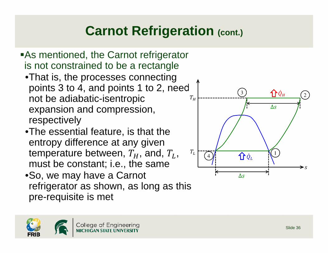
As mentioned, the Carnot refrigerator is not constrained to be a rectangle•That is, the processes connecting points 3 to 4, and points 1 to 2, need not be adiabatic-isentropic expansion and compression, respectively
•The essential feature, is that the entropy difference at any given temperature between, , and, , must be constant; i.e., the same
•So, we may have a Carnot refrigerator as shown, as long as this pre-requisite is met
Slide 36

Carnot Refrigeration (cont.)
These curves are reminiscent of constant pressure lines, which are a practical process pathHowever, it should be stated that, if for example, the path from 1 to 2 is a constant pressure process, to meet the pre-requisite of a constant entropy difference at any given temperature, the path from 3 to 4 is not a constant pressure (unless it is a perfect ideal gas; which has no two-phase region)Although, the process line from point 3 to 4 passes through the two-phase region, for cryogenic fluids, this overlap is a very small fraction of the total temperature spanSince these slanted lines are not adiabatic-isentropic paths, there is heat transfer between these counter-flowing streams
Slide 37

Carnot LiquefierIdeal Liquefier, or Carnot Liquefier•A liquefaction load is fundamentally different than a refrigeration load, in that the refrigeration temperature of the gas being liquefied continuously varies
•The diagram depicts this idea – there are many Carnot refrigerators ( ) operating over a small temperature span ( to
) to cool the mass flow ( )
Slide 38

Carnot Liquefier (cont.)
If we were to use a very large number of these Carnot refrigerators, so that the temperature span was, , the reversible work required for each of these would be,
1
We will return to this after discussing the Carnot Liquefier
Slide 39

Carnot Liquefier (cont.)
Carnot Liquefier:Pts. 1 to 2: An amount of gas, , is compressed reversibly-isothermally from the environment pressure and temperature ( and
, say 1 atm, and 300 K) to some (high) pressure•Note: this requires input power,
, and, , amount of heat is rejected to the environment
Pts. 2 to 3: Adiabatic-isentropic expansion to the saturated liquid condition; so, (100%) saturated liquid is produced at a rate of,
Slide 40
Carnot Liquefier (cont.)
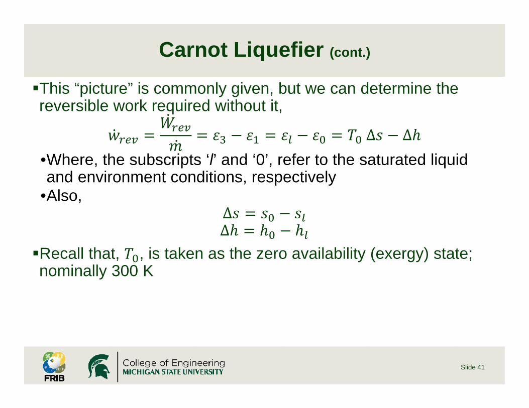
This “picture” is commonly given, but we can determine the reversible work required without it,
Δ Δ•Where, the subscripts ‘l’ and ‘0’, refer to the saturated liquid and environment conditions, respectively
•Also,ΔΔ
Recall that, , is taken as the zero availability (exergy) state; nominally 300 K
Slide 41

Carnot Liquefier (cont.)
Below are some results for a number of refrigerants:
Note that we will reference to 1 atm for the saturated condition, since this is taken as the zero availability (exergy) reference
Slide 42
Name Symbol R # MW Tsat at p0 h s (T0·s) wrev[g/mol] [K] [J/g] [J/g-K] [J/g] [J/g]
Refrigerant-11 CCl3F R-11 137.4 296.8 183.2 0.617 185.2 2.0Refrigerant-134A C2H2F4 R-134a 102.0 246.9 260.5 1.039 311.6 51.0Refrigerant-12 CCl2F2 R-124 120.9 243.4 199.3 0.805 241.5 42.2Ammonia NH3 R-717 66.05 239.8 1502 6.204 1861 359.2Refrigerant-22 CHClF2 R-22 86.48 234.3 274.9 1.160 348.0 73.1Xenon Xe 131.3 165.0 118.5 0.682 204.7 86.2Krypton Kr R-784 83.80 119.8 153.6 1.135 340.5 186.9Methane CH4 R-50 16.04 111.7 914.0 6.688 2006 1092Oxygen O2 R-732 32.00 90.19 406.1 3.471 1041 635.2Argon Ar R-740 39.95 87.28 273.7 2.504 751.2 477.5Nitrogen N2 R-728 28.01 77.31 433.6 4.011 1203 769.8Neon Ne R-720 20.18 27.09 368.6 5.684 1705 1337Deuterium D 4.028 23.66 2271 30.44 9132 6861Hydrogen H2 R-702 2.016 20.28 4455 56.80 17028 12573Helium-4 He R-704 4.003 4.22 1564 28.01 8403 6839
Carnot Liquefier (cont.)
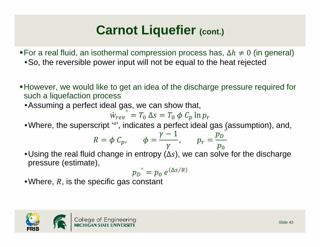
For a real fluid, an isothermal compression process has, Δ 0 (in general)•So, the reversible power input will not be equal to the heat rejected
However, we would like to get an idea of the discharge pressure required for such a liquefaction process•Assuming a perfect ideal gas, we can show that,
° Δ ln•Where, the superscript ‘°’, indicates a perfect ideal gas (assumption), and,
,1,
°
•Using the real fluid change in entropy (Δ ), we can solve for the discharge pressure (estimate),
° ⁄
•Where, , is the specific gas constant
Slide 43

Carnot Liquefier (cont.)
Below are some results for a number of refrigerants:
This table clearly demonstrates that this is not a practical cycle; however, it establishes the minimum input power required to liquefySuch a cycle gives us a minimum mass flow rate
Slide 44
Name Symbol R # MW [g/mol] Tsat [K] at p0 pD° [atm]
Refrigerant-11 CCl3F R-11 137.4 296.8 26920Refrigerant-134A C2H2F4 R-134a 102.0 246.9 342652Refrigerant-12 CCl2F2 R-124 120.9 243.4 121303Ammonia NH3 R-717 66.05 239.8 2.53E+21Refrigerant-22 CHClF2 R-22 86.48 234.3 173849Xenon Xe 131.3 165.0 47665Krypton Kr R-784 83.80 119.8 93014Methane CH4 R-50 16.04 111.7 401589Oxygen O2 R-732 32.00 90.19 633053Argon Ar R-740 39.95 87.28 167787Nitrogen N2 R-728 28.01 77.31 740624Neon Ne R-720 20.18 27.09 978649Deuterium D 4.028 23.66 2541575Hydrogen H2 R-702 2.016 20.28 948114Helium-4 He R-704 4.003 4.22 717726
Carnot Liquefier (cont.)
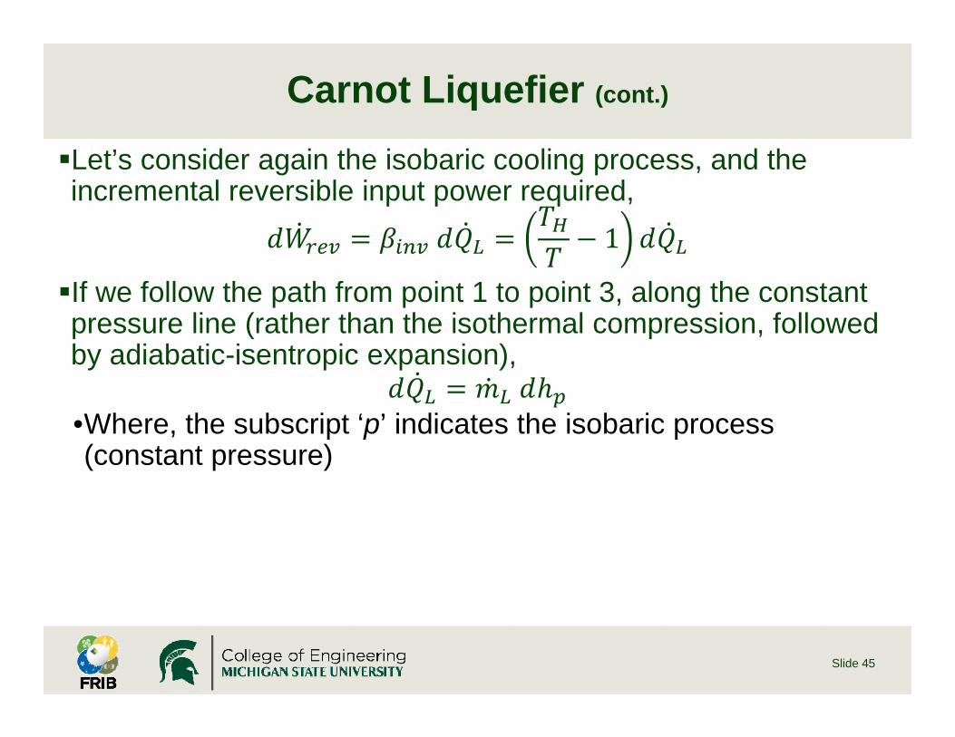
Let’s consider again the isobaric cooling process, and the incremental reversible input power required,
1
If we follow the path from point 1 to point 3, along the constant pressure line (rather than the isothermal compression, followed by adiabatic-isentropic expansion),
•Where, the subscript ‘p’ indicates the isobaric process (constant pressure)
Slide 45

Carnot Liquefier (cont.)
Recalling the relation,
This reduces to,
So,
1
Integrating this,
This is simply the area enclosed by points, 1-2-3-4-1; where point 4 is the saturated vapor condition
Slide 46

Carnot Liquefier (cont.)
Also, since the total heat removed,
We can see that this is comprised of two components; the sensible portion from point 1 to 4, and the latent portion from 4 to 3,
•Where, , is the enthalpy at, , ; , is the saturated
vapor enthalpy; , is the latent heat
Slide 47

Carnot Liquefier (cont.)
Reversible input power required for the latent portion is what we found for the case of Carnot refrigerationReversible input power required for both sensible and latent portions is what we found for the case of the Carnot liquefier•e.g., Helium at 1 g/s
»Sensible enthalpy (300 K to 4.22 K at 1 atm) is (1449 – 20.7 =)1428 J/g, and the latent heat is 20.7 J/g
»Reversible input power for sensible cooling is (6839 – 1449 =) 5390 W/(g/s), and for the latent cooling 1449 W/(g/s)
»So, even though the latent cooling is only ~1% of the cooling load, it is 21% of the total reversible input power
»This is a consequence of the quality of thermal energy expressed in the 2nd Law
Slide 48
Cryogenic CyclesIn summary for isothermal refrigeration vs. liquefaction•The essence of a refrigerator, supporting only an isothermal refrigeration load, is that there is no sensible cooling needed for the load»So, the temperature where the cooling occurs does not vary (for the isothermal load)
•The essence of a liquefier, supporting only a liquefaction load, is that the sensible cooling is the (overwhelming) dominate cooling needed»Although, the latent heat must be overcome, this is quite small for most cryogenic cycles compared to the sensible enthalpy
»So, the temperature where the cooling occurs varies continuously, from the make-up gas temperature, down to the saturated liquid temperature
Slide 49

Cryogenic Cycles (cont.)
Efficiency of helium refrigeration vs. size:•Large refrigerators tend to be more efficient than smaller ones; a typical ‘large’ size is ~18 kW at 4.5 K
Slide 50

Model Real CyclesReal Gas Helium Refrigeration:
To understand the essential features of a real gas helium refrigerator, we will examine two process cases:
•Case 1 – Irreversible process, ideal-practical (and a minimum amount of) equipment
•Case 2 – Reversible process, non-practical equipment
Slide 51

Model Real Cycles (cont.)
Case 1:•Pts. 1 to 2: Isothermal compression•Pts. 2 to 3 and 5 to 1: Counter-flow heat exchange using a 100% effective heat exchanger; with no pressure drop
•Pts. 3 to 4: Isentropic-adiabatic expansion•Pts. 4 to 5: Isothermal refrigeration load (saturated liquid to saturated vapor)
Slide 52

Model Real Cycles (cont.)
Case 1 (continued):•Stream temperature difference at cold-end of heat exchanger is ~3.5 K (i.e.,
7.69K)•Note: since the heat exchanger is 100% effective, the stream temperature at the warm-end is 0 K
•Pressure at pt. 3 to the inlet of the isentropic expander is ~70 atm
Slide 53

Model Real Cycles (cont.)
Case 1 (continued):
We can make several observations:•This is not a reversible process (due to the heat exchanger finite stream temperature difference, except that the warm-end)
•Work extraction is needed at the cold-end; as opposed to being distributed or at the warm-end
•This is to gain the latent heat; however, ~43.4 W/(g/s) of work extraction is needed (rather than 20.7 W/(g/s) for the latent heat at 4.22 K), since this process is not reversible
•If the expander work is recovered, a specific input power of, 2626 W/(g/s) would be required (as opposed to 1449 W/(g/s) for a reversible process)
•Or, an inverse coefficient of, ~127 W/W (as compared to, ~70 W/W for a reversible process)
•This configuration represents a minimum of equipment
Slide 54

Model Real Cycles (cont.)
Case 2:•Recall that if, for the counter-flow heat exchange, we keep the entropy difference equal at every temperature level, the process is reversible
Slide 55

Model Real Cycles (cont.)
Case 2 (continued):• If we follow the 1 atm isobar for the return stream, and then ‘map’ out the supply stream (being cooled by the return stream), we find that the pressure of this stream is not constant (and in fact cannot be so)
•At 300 K, it begins at 10.58 atm, and does not begin to rapidly drop until ~40 K
Slide 56
Model Real Cycles (cont.)
Case 2 (continued):
We can make several observations:•This is a reversible process; requiring 1449 W/(g/s), or, ~70 W/W, the same as the Carnot refrigerator
•This is not a practical process, since there is simultaneous counter-flow heat exchange and work extraction
•Most of the work extracted is below ~40 K (where the pressure starts to drop rapidly)
•The total (net) work extracted is 23.9 W/(g/s), which is, 3.1 W/(g/s) higher than the latent heat due to additional input power required for the real gas isothermal compression process
Slide 57

Model Real Cycles (cont.)
Real Gas Helium Refrigeration:
Both of these cases tell us three important aspects required by a refrigerator:•Vast majority of the required work extraction (by adiabatic expansion) is needed at the cold-end of the refrigerator; i.e., below ~40 K
•A (thermally) ‘long’ and effective heat exchanger is crucial (for good efficiency)
•‘Recycle’ mass flow should be avoided (or at least minimized); i.e., all of the compressor mass flow should ideally go to the refrigeration load for an idealized, but practical, process
Slide 58

Model Real Cycles (cont.)
Real Gas Helium Liquefaction:
Recall that a practical liquefaction process requires continuous cooling of the flow being liquefied (the isobaric path of the Carnot liquefier)This means there is (semi-)continuous work being extracted from the high availability fluid to cool the make-up (i.e., fluid being liquefied)As such, real gas effects play a significantly lesser role (for helium) systems over a majority of the temperature that the fluid is being cooled
Slide 59
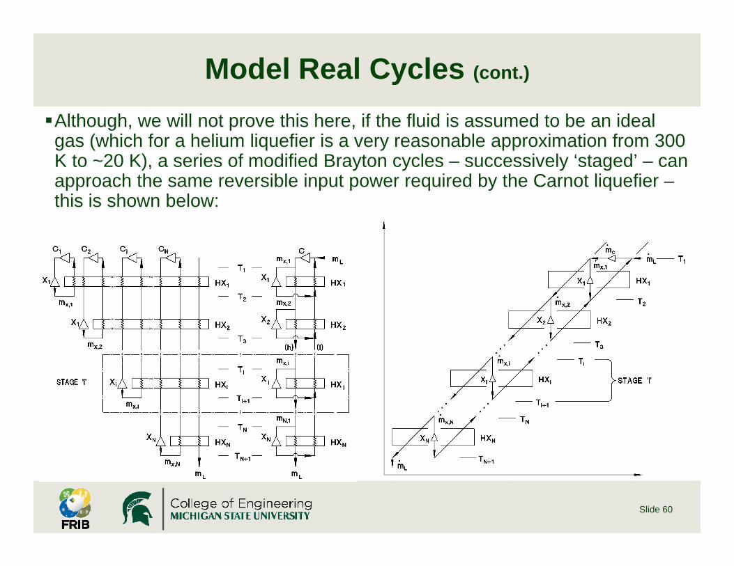
Model Real Cycles (cont.)
Although, we will not prove this here, if the fluid is assumed to be an ideal gas (which for a helium liquefier is a very reasonable approximation from 300 K to ~20 K), a series of modified Brayton cycles – successively ‘staged’ – can approach the same reversible input power required by the Carnot liquefier –this is shown below:
Slide 60

Model Real Cycles (cont.)
We can observe that:•There is work being extracted over the entire temperature range•Heat exchangers are assumed to be 100% effective; so, that the stream temperature difference (‘pinch’) between each expansion stage is zero
•Each expander is isentropic•The number of expansion stages ( ) is directly related to the total temperature ratio (Θ ⁄ ) and the pressure ratio of the (h) to (l) streams (Π ⁄ )
•By inspection, we can see that the temperature ratio of each expansion stage ( ⁄ ) is,
Θ ⁄ Π•So,
ln Θln
lnΘ lnΠ
•With,1 ⁄
Slide 61

Model Real Cycles (cont.)
Additionally, the mass flow through each expander is the same (i.e., ), and equal to the mass flow being liquefied ( )So, the compressor mass flow rate is,
1 Consequently, the heat exchangers are balanced (i.e., have equal stream capacities); i.e.,
→•Where, , , and, ,
For real cycles, since the expanders are not isentropic and the heat exchangers not perfect (i.e., 100% effective), we introduce and additional heat exchanger in between expansion stages
Slide 62

Model Real Cycles (cont.)
For this arrangement, it can be shown that, if the,•Heat exchangers were 100% effective (i.e., Δ , , , 0), and,
•Each expander had the same isentropic efficiency ( , , but less than 100%)
•As before, the temperature ratio for each expansion stage (
, ,⁄ ) is equal, and,•The expander mass flow rate for each stage ( , ) is equal
However, the mass flow for each expander is higher than the mass flow being liquefied (as would be expected)
Slide 63
Model Real Cycles (cont.)
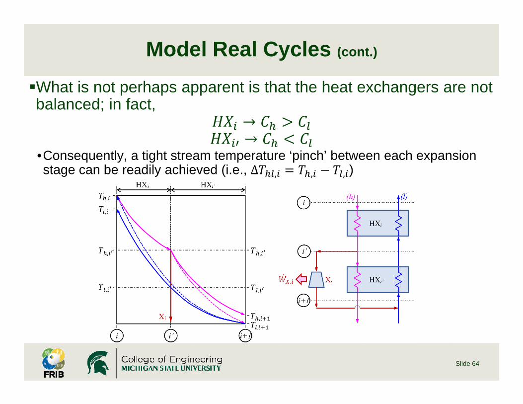
What is not perhaps apparent is that the heat exchangers are not balanced; in fact,
→→
•Consequently, a tight stream temperature ‘pinch’ between each expansion stage can be readily achieved (i.e., ∆ , , , )
Slide 64

Model Real Cycles (cont.)
It can be shown that:•Expander temperature ratio,
, 1 1 Π•Ratio of expander mass flow to liquefaction,
,,
•Ratio of expander mass flows,,
,1
•Compressor mass flow,∑ , 1 ,
A more general solution for a practical liquefier, that has a concurrent isothermal refrigeration load is available:•(“Simplified helium refrigerator cycle analysis using the ‘Carnot Step’, http://aip.scitation.org/doi/abs/10.1063/1.2202630)
Slide 65

Model Real Cycles (cont.)
So, to contrast with a helium refrigerator (handling an isothermal refrigeration load), for good efficiency:
•Many, high efficiency, expanders are necessary – but the heat exchanger requirement is not as strict
•Also, a large portion of the compressor mass flow is ‘recycled’ through the expansion stages; with only a small portion going to the liquefaction load
Slide 66
Model Real Cycles (cont.)
These differences impose quite different requirements on the components used in the refrigerator vs. the liquefier
As can be shown, approx. 100 W of refrigeration at 4.5 K is exergetically equivalent to 1 g/s of liquefaction (at 4.5 K); if the expander output power is recovered (otherwise it is, approx. 120 W of refrigeration per 1 g/s of liquefaction)
However a liquefier, will not necessarily produce an equivalent amount of refrigeration compared to its liquefaction capacity
And, a refrigerator, will not necessarily produce an equivalent amount of liquefaction compared to its refrigeration capacity
Slide 67
Model Real Cycles (cont.)
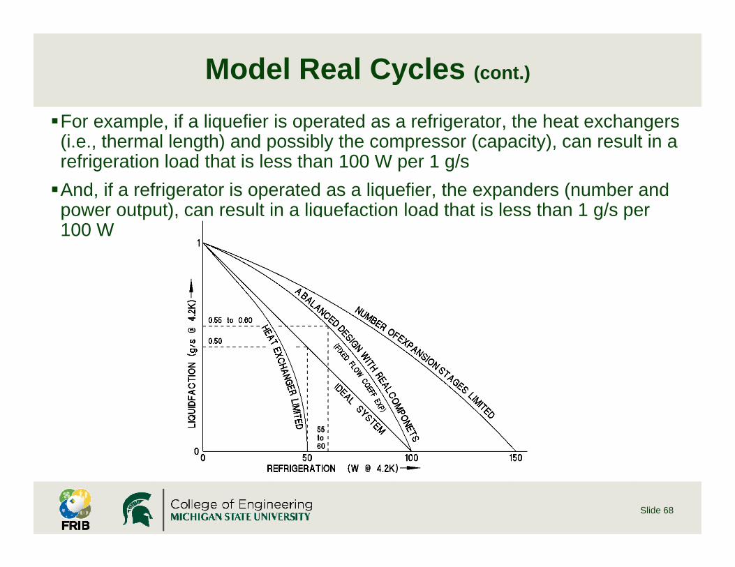
For example, if a liquefier is operated as a refrigerator, the heat exchangers (i.e., thermal length) and possibly the compressor (capacity), can result in a refrigeration load that is less than 100 W per 1 g/sAnd, if a refrigerator is operated as a liquefier, the expanders (number and power output), can result in a liquefaction load that is less than 1 g/s per 100 W
Slide 68

JT StageJoule-Thompson (JT) Stage:As discussed the JT stage is dominated by, and in fact dependent on (if it is to function at all), real fluid – non-ideal gas – propertiesRecall, the Joule-Thompson coefficient – change in temperature w.r.t. pressure at constant enthalpy
For an ideal gas, the JT-coefficient is zeroFor this to be non-zero, the fluid must be non-ideal; specifically, the fluid is comprised of finite volume molecules that experience inter-molecular forcesFortunately, real fluids are non-ideal
Slide 69
JT Stage (cont.)
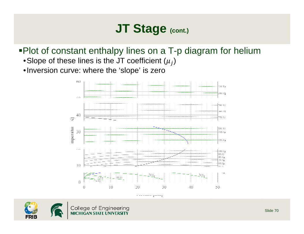
Plot of constant enthalpy lines on a T-p diagram for helium•Slope of these lines is the JT coefficient ( )• Inversion curve: where the ‘slope’ is zero
Slide 70
JT Stage (cont.)
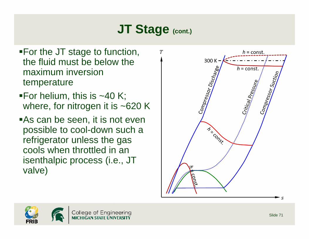
For the JT stage to function, the fluid must be below the maximum inversion temperatureFor helium, this is ~40 K; where, for nitrogen it is ~620 KAs can be seen, it is not even possible to cool-down such a refrigerator unless the gas cools when throttled in an isenthalpic process (i.e., JT valve)
Slide 71