phylogenetic analysis of hiv samples from a single host

Phylogenetic Analysis of HIVSamples from a Single Host

Master Thesis

Rounak Vyas

November 20, 2011

Advisors: Prof. Niko Beerenwinkel, Dr. Osvaldo Zagordi

Computational Biology Group, ETH Zurich

Contents

Contents i

1 Introduction 11.1 AIDS . . . . . . . . . . . . . . . . . . . . . . . . . . . . . . . . . 11.2 HIV . . . . . . . . . . . . . . . . . . . . . . . . . . . . . . . . . . 21.3 Longitudinal Studies . . . . . . . . . . . . . . . . . . . . . . . . 41.4 HIV Sequencing . . . . . . . . . . . . . . . . . . . . . . . . . . . 61.5 Recent Studies of HIV-1 . . . . . . . . . . . . . . . . . . . . . . 6

2 Materials and Methods 92.1 Patient History . . . . . . . . . . . . . . . . . . . . . . . . . . . 92.2 Data Pre-processing . . . . . . . . . . . . . . . . . . . . . . . . . 112.3 Entropy Analysis . . . . . . . . . . . . . . . . . . . . . . . . . . 112.4 Recombination Analysis . . . . . . . . . . . . . . . . . . . . . . 122.5 Molecular Clock Estimation . . . . . . . . . . . . . . . . . . . . 132.6 Poisson Fitter . . . . . . . . . . . . . . . . . . . . . . . . . . . . 162.7 Sliding MinPD . . . . . . . . . . . . . . . . . . . . . . . . . . . . 172.8 Rate of synonymous and nonsynonymous substitutions . . . 18

3 Results 213.1 Entropy Analysis . . . . . . . . . . . . . . . . . . . . . . . . . . 213.2 Molecular Clock Rate Estimation and Phylogenetic Tree Con-

struction . . . . . . . . . . . . . . . . . . . . . . . . . . . . . . . 233.3 Founder Virus Analysis . . . . . . . . . . . . . . . . . . . . . . 283.4 Demographic Reconstruction . . . . . . . . . . . . . . . . . . . 343.5 Sliding MinPD . . . . . . . . . . . . . . . . . . . . . . . . . . . . 353.6 Conclusions . . . . . . . . . . . . . . . . . . . . . . . . . . . . . 39

Bibliography 40

i

Chapter 1

Introduction

The earliest well documented incident of AIDS dates back to the 1980’s.Since then, more than 25 million people have died from AIDS [4]. TheWorld Health Organization has now declared AIDS a pandemic and sincereefforts are underway around the world to identify an effective cure for thiscondition.

1.1 AIDS

As the name suggests, Acquired Immunodeficiency Syndrome (AIDS) is acondition wherein the patient’s immune system becomes severely compro-mised, enabling opportunistic infections such as pneumonia, tuberculosis,herpes, and others. These infections ultimately result in the death of thepatient. Clinically, AIDS is described as an advanced stage in an infectioncaused by Human Immunodeficiency Virus (HIV) wherein the CD4+ cellcount drops below the critical level. CD4+ cells are a special class of whiteblood cells which play a major role in recognizing foreign antigens (like bac-teria and viruses) within the body [12]. In their absence, the immune systemis not able to recognize and clear these foreign agents leading to sustainedinfections.

HIV infection can only be contracted from another infected individual throughexchange of body fluids like blood, genital fluids and breast milk. Chanceexchange of these takes place when the individuals share needles of an in-jection or engage in unprotected sexual intercourse. The infection cannot beacquired by ingestion of the virus.

An individual may remain HIV positive for several years before becomingan AIDS patient. After the onset of AIDS, the patient’s life span shortens to 8to 12 months [19]. Current therapies are able to significantly increase the lifespan of the infected individuals by delaying the onset of AIDS. Most of these

1

1.2. HIV

therapies act by interfering with one of the crucial steps in replication, entryor release of the virus from the infected cell. However, due to the unusuallyhigh rate of mutation in HIV, it is able to quickly develop resistance againstthese therapies and flourish again. Hence there is presently no cure for AIDS[29].

AIDS is not a disease that targets a specific organ, but a condition charac-terized by progressive immune failure leading to infections in several or-gans. To develop an effective therapy, it is imperative to gain insight onthe processes through which the virus evolves to establish a nonperishablepopulation within the host. Of particular interest are the evolutionary pat-tern the virus undergoes while subjected to selective pressures of the hostimmune system, and the development of viral drug resistance. A detailedunderstanding of these processes may offer insight into the development ofeffective treatment strategies.

1.2 HIV

The Human Immunodeficiency Virus belongs to the family of retroviruses[3], RNA viruses that use reverse transcriptase to encode their genetic ma-terial into DNA only within a host cell. It is known to cause AcquiredImmunodeficiency Syndrome [34]. There are two prominent types knownas HIV-1 and HIV-2, differing in their virulence, infectivity, and prevalence[15]. These have originated from the Simian Immunodeficiency Virus sub-types cpz and smm and infect chimpanzees and old world monkeys respec-tively. In this report we focus on HIV-1 as this is the virus type with whichboth patients were infected.

Figure 1.1: Diagram of Human Immunodeficiency Virus [1]

The virus has of two identical copies of the complete genome encoded ontwo positive single RNA strands and consists of nine genes encoding 19 vi-

2

1.2. HIV

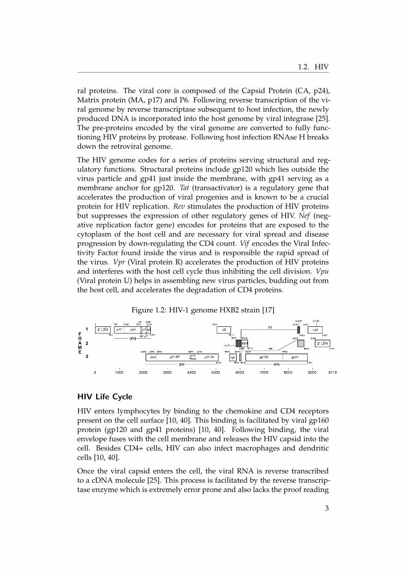
ral proteins. The viral core is composed of the Capsid Protein (CA, p24),Matrix protein (MA, p17) and P6. Following reverse transcription of the vi-ral genome by reverse transcriptase subsequent to host infection, the newlyproduced DNA is incorporated into the host genome by viral integrase [25].The pre-proteins encoded by the viral genome are converted to fully func-tioning HIV proteins by protease. Following host infection RNAse H breaksdown the retroviral genome.

The HIV genome codes for a series of proteins serving structural and reg-ulatory functions. Structural proteins include gp120 which lies outside thevirus particle and gp41 just inside the membrane, with gp41 serving as amembrane anchor for gp120. Tat (transactivator) is a regulatory gene thataccelerates the production of viral progenies and is known to be a crucialprotein for HIV replication. Rev stimulates the production of HIV proteinsbut suppresses the expression of other regulatory genes of HIV. Nef (neg-ative replication factor gene) encodes for proteins that are exposed to thecytoplasm of the host cell and are necessary for viral spread and diseaseprogression by down-regulating the CD4 count. Vif encodes the Viral Infec-tivity Factor found inside the virus and is responsible the rapid spread ofthe virus. Vpr (Viral protein R) accelerates the production of HIV proteinsand interferes with the host cell cycle thus inhibiting the cell division. Vpu(Viral protein U) helps in assembling new virus particles, budding out fromthe host cell, and accelerates the degradation of CD4 proteins.

Figure 1.2: HIV-1 genome HXB2 strain [17]

HIV Life Cycle

HIV enters lymphocytes by binding to the chemokine and CD4 receptorspresent on the cell surface [10, 40]. This binding is facilitated by viral gp160protein (gp120 and gp41 proteins) [10, 40]. Following binding, the viralenvelope fuses with the cell membrane and releases the HIV capsid into thecell. Besides CD4+ cells, HIV can also infect macrophages and dendriticcells [10, 40].

Once the viral capsid enters the cell, the viral RNA is reverse transcribedto a cDNA molecule [25]. This process is facilitated by the reverse transcrip-tase enzyme which is extremely error prone and also lacks the proof reading

3

1.3. Longitudinal Studies

capacity leading to a misincorporation rate of 10−4 to 10−5 per base or ap-proximately one mis-incorporation per genome per replication cycle [38].The cDNA and its complement form a double stranded viral DNA whichis then transported into the cell nucleus where it is subsequently integratedinto the host genome with the help of integrase viral enzyme [25].

Once incorporated, viral DNA requires cellular transcription factors to en-code for viral proteins. During viral replication, the pro-viral DNA is tran-scribed into mRNA which is spliced and then transported to the cytoplasmwhere it is translated into viral proteins (mainly Tat and Rev Proteins). Revprotein accumulates in the nucleus and inhibits mRNA splicing and the un-spliced full length mRNA leave the nucleus to enter the cytoplasm [32]. Thefull length mRNA is actually the viral genome which binds to Gag proteinand is packaged into new viral packets. After processing by the host en-doplasmic reticulum gp160 is transported to the plasma membrane wheregp41 anchors gp120 to the membrane of the infected host cell. The viralcapsid then assembles and buds out of the cell to infect other cells [25].

The high rate of mutation in HIV is due to the high error rate of the reversetranscriptase enzyme while transcribing the viral RNA genome into a DNAsequence that can be incorporated in the host cell genome for coding viralproteins [5]. Along with a high misincorporation rate of approximately onebase per replication, reverse transcriptase also lacks proof-reading activityrendering it unable to check and rectify copy mistakes, often resulting inseveral slightly different copies of HIV within a single patient. Distinct viralpopulations are referred to as ”quasispecies”, and each genetically distinctindividual is referred as a haplotype.

1.3 Longitudinal Studies

Due to the prohibitively expensive nature of prospective HIV screening, HIVstudies are generally only performed on high risk population groups, suchas within a prison. Combined with additional ethical considerations, theresult is that most studies enroll patients that are already symptomatic. Inalready symptomatic populations the viral load is already established andthus is of little insight into the dynamics of the pre-seroconversion phase, i.e.before any viral antibody production has taken place.

To develop insight into the temporal evolution of the virus within a host,longitudinal studies of patient populations are of critical importance. Longi-tudinal studies combine data collected at multiple examinations at intervalsbetween minutes and years to afford a more comprehensive insight into theviral dynamics than is possible through examinations at a single time pointalone.

4

1.3. Longitudinal Studies

Figure 1.3: HIV Life Cycle [6]

While longitudinal studies are clearly desirable, they also present technicalchallenges such as censoring of events due to the relocation, death or dis-enrollment of cohort members. Additionally, changing patient habits and alifestyle choice can complicate analysis. Lastly, longitudinal studies are nec-essarily more involving and therefore more expensive than single time-pointstudies.

5

1.4. HIV Sequencing

1.4 HIV Sequencing

Traditional Sanger-based sequencing method only read the consensus ge-nomic sequence of heterogeneous viral populations [36], obfuscating thegenomic variability present in the population which is of potential impor-tance for identifying gradually-fixating resistance mutations. Next Genera-tion Sequencing (NGS) technologies represent an improvement over Sangersequencing and facilitate the sequencing of distinct haplotypes within a sam-ple [30]. However, NGS reads are error-prone and require sophisticatedprocessing techniques to create error-free haplotype reconstruction and fre-quency estimation. Currently, haplotypes with frequencies as low as 0.05%can be estimated with 99% confidence [24].

1.5 Recent Studies of HIV-1

In 1999 R. Shankarappa et al. conducted a landmark study investigating theevolution of HIV within an infected individual prior to the onset of AIDS[22]. They studied the evolution of C2-V5, a high mutation region of theHIV-1 env gene, in nine patients over six to twelve years. They estimatedthe viral diversity within and between time points, identified mutations con-ferring the viral strain any fitness advantage, and characterized the existenceof three distinct phases: the early phase with linear increase in diversity anddivergence from the founder virus strain, an intermediate phase with linearincrease in divergence but stabilization or decline in diversity, and a latephase with stabilization in the divergence and continued decrease in diver-sity.

More recently, Poon et al, used longitudinal deep sequencing data with coa-lescent analysis to estimate the date of HIV infection [26]. Time of infectionwas estimated using the time to most recent common ancestor (TMRCA) ofa time-calibrated phylogenetic tree relating sequences from all time points.This is justified by the argument that most HIV infections are established bya single viral strain due to bottlenecks during transmission [39, 13]. 19 HIVpositive individuals were followed and 7 genomic regions were analyzed.The authors compared the estimated time since infection from experimen-tal methods to TMRCA estimates obtained with the BEAST software library.They observed a stronger correlation between clinical and computational es-timates for TMRCA in highly variable regions of HIV genome (such as env)relative to that in conserved regions such as pol. The reduced correlation inthe conserved regions is thought to be due to a possible overestimation oftime scales due to the increased sensitivity of the coalescent based methodstowards the sampled genetic variation. Consequently, sequences with highdivergence were found to be ideal for calibrating the evolutionary clock. Inthe case of a multiple founder virus infection, this method was found to

6

1.5. Recent Studies of HIV-1

overestimate the infection time.

In the same month another interesting study was published by a differentauthor, Suzanne English, et al. [23]. This discussed the construction of thetransmission history of HIV-1 infected individuals using Phylogenetic meth-ods. It showed that the diversity is fairly limited in the early phase of theinfection and is even compatible with the transmission of a single viral vari-ant. It also provided evidence to support the idea that a single donor canin principle transmit two distinct variants to two different individuals in asmall time span of few hours. The transmission history was constructedusing the Bayesian and Maximum likelihood approach. Env, gag and pol re-gions were used for this analysis. The inter host genetic diversity predictionsproportionately varied depending on the extent of conservation observed inthe region used for its prediction. Highest diversity was predicted usingenv gene (least conserved) followed by pol gene and then gag gene. Trans-mission history was constructed using the inter-host variation observed inthese three regions. BEAST software was used for carrying out this analysis.

A temporal study on HIV-1 was undertaken by G. Achaz et al and pub-lished in 2004 [11]. This study was conducted using gag-pol sequence datacollected over time from two chronically infected individuals to estimate thepopulation structure and the neutral mutation rate of this region per site pergeneration. Neutral coalescent models were used for the analysis. For thegenealogy construction, coalescent approach identical to the one proposedby Felsenstein 1999 was used. 19 time points collected over a period of 4years were used for the analysis. This compensated for the low mutationrate in the sequences.

A longitudinal study to understand the viral evolution in early Acute Hep-atitis C Virus infection was carried out by Bull RA, Luciani F, McElroy K,Gaudieri S, Pham ST, et al. published in 2011 [9]. We discuss this paperin greater detail due to the parallelism with our study. This study aimedat identifying genetic variants as low as 0.1% frequency and subsequentlyquantify them over the course of infection. They also identified two sequen-tial bottlenecks that occurred early in infection. BEAST software was used toestimate the changes in the effective population size of the virus populationover time. It was also used to construct ancestor descendant relationshipswith the viral samples from different time points. The rate of evolution forthe virus was also estimated during this analysis. In depth nonsynonymousand synonymous substitution analysis was carried out to identify any vis-ible pattern of change. Entropy changes were measured across the wholegenome and across patients which indicated non-uniform evolution of HCVacross the genome and over time. Single founder virus hypothesis weretested for infection using the freely available tool called as Poisson Fitter onthe HIV database.

7

1.5. Recent Studies of HIV-1

Several other time series data analysis on HIV positive patients have beencarried out for identifying/understanding the order in which resistance mu-tations are accumulated when the patient is placed under a drug therapy.However, we do not discuss these since our patients did not show any drugresistance even after the therapy was discontinued.

8

Chapter 2

Materials and Methods

2.1 Patient History

HIV samples were collected from two patients enrolled at the department ofinfectious diseases at Universitatspital Zurich. The protease coding regionof HIV was deep-sequenced and analyzed. This region was chosen for thestudy since both the patients were treated with a protease inhibitor drug.

Patient I.D.123

Figure 2.1: Viral load in patient I.D. 123

This patient was a part of the Primary HIV Infection study which empha-sizes on beginning the treatment in the early phase of infection and thendiscontinuing it. It is based on the assumption that the patient is likely tocontrol the virus when the treatment is started early. However, most patients

9

2.1. Patient History

Table 2.1: Sample collection time points, patient I.D.123

Sr.No. Sample Name Sample Collection Date1 PR1 12.12.20032 PR 2 15.12.20053 PR 28 30.05.20064 PR 3 14.08.2007

suffer from a viral rebound, like patient 123. As can be seen in figure 2.1,four samples over a period of 3.74 years were sequenced from the patientafter being tested as HIV positive. These samples have been marked in red.The regions marked as ART in figure 2.1 show the periods of treatment withLopinavir, an anti-retroviral drug. The exact dates of sample collection canbe seen in table 2.1

Patient I.D.181

Figure 2.2: Viral load in patient I.D.181

The patient remained untreated until almost an year after being tested HIVpositive. During this phase, the viral load in blood plasma was regularlymonitored. Samples from three time points marked with red in figure 2.2were deep-sequenced and analyzed. The exact dates of sample collectionhave been mentioned in table 2.2.

10

2.2. Data Pre-processing

Table 2.2: Sample collection time points, Patient I.D.181

Sr.No. Sample Name Sample Collection Date1 PR4 28.09.20052 PR 5 15.03.20063 PR 6 08.09.2006

2.2 Data Pre-processing

Haplotype reconstruction and error correction was performed using ShoRAH[24]. The output file contained haplotype sequences in FASTA format. Theheader of each haplotype contained two numbers. First number showed ourconfidence in the haplotype sequence on a scale of 0 to 1. The other num-ber could be used to calculate the frequency of the haplotype in the samplepopulation. It showed the number of times the sequences constituting thehaplotype were sequenced. It is known as the average read number of ahaplotype.

These files often contained over a hundred sequences with only a few hav-ing a high read count and confidence. For a meaningful analysis, these fileswere filtered to select sequences with a confidence of over 0.9. This reducedthe number of haplotypes to one quarter or less. The threshold was chosento optimize the number of sequences for analysis. Too few sequences wouldnot contain enough information for the analysis and too many would cer-tainly add noise to the result. This cutoff returned a reasonable number ofhaplotypes.

Since a functional protease is fundamental for HIV, any gaps present in thehaplotype sequences were assumed to be sequencing errors. The haplotypesfrom a single run were used to first construct a consensus sequence usingthe Biopython EMBOSS tool known as “Cons”. Any gaps present in the con-sensus sequence were filled using HXB2 protease reference sequence. Theconsensus sequence was then used to fill the gaps present in the haplotypesequences. The reading frame of every haplotype was also ensured to startat the first nucleotide position. A python script was written for performingall the above tasks.

2.3 Entropy Analysis

HIV constantly accumulates mutations to cope with the selective forces be-ing exerted by the immune system and drug treatments. The nucleotidesites that accumulate these mutations are mainly responsible for renderingthe virus resistant to different therapies. In order to improve our current

11

2.4. Recombination Analysis

methods, it would be fruitful to identify these sites and also have an insighton how these sites maintain diversity in the viral population. For this pur-pose we calculate entropy for every time point dataset and try to identifyany visible spatial or temporal patterns.

Entropy of a position in a sequence depicts the uncertainty associated withthe nucleotide present at the site. High entropy indicates that the site canhave variable nucleotides.

Let X be a discrete random variable ( bases while considering nucleotides,amino acids while considering proteins), taking a finite number of possiblevalues x1, x2, . . . , xn with probabilities p1, p2, . . . , pn such that pi ≥ 0, i =1, 2 . . . , n and ∑n

i=1 pi = 1. The entropy is then given by

Hn(p1, p2, ..., pn) = −n

∑i=1

pilogb pi

Here b is the base of the logarithm. A simple python script was writtento calculate and plot the entropy at every position in the alignment, weused natural logarithm for our calculations. When deep-sequencing datawas submitted as an input, the script could take into account the averagenumber of reads while calculating the entropy at every position.

2.4 Recombination Analysis

Recombination plays a crucial part in the evolution of retroviruses and ismore prevalent in conserved regions [7]. Since we use a fairly conservedHIV region for our analysis, we performed a recombination detection study.If an alignment contains recombinant sequences then relationships betweendifferent segments of the alignment cannot be described using a single phy-logenetic tree. To unfold the true evolutionary relationships, it is imperativeto identify the recombination break points and partition the alignment intothe number of observed recombinant sets and then depict the evolutionaryrelationships in each of these partitions using a separate phylogenetic tree.If recombination events are not taken into account during a phylogeneticanalysis, then the results are most likely to be meaningless.

We used Recombination Identification program [37] which has been developedto specifically detect recombinants in HIV-1 nucleotide sequences. It acceptsa set of nucleotide sequences from a single viral genomic region collectedfrom a single patient as an input. The program requires a background se-quence which is essentially the consensus sequence of the genomic regionthat is to be analyzed. This can be selected from the available list in theprogram; alternatively the user is free to submit a consensus sequence with

12

2.5. Molecular Clock Estimation

the nucleotide data. In the latter case, the consensus should be aligned tothe rest of the sequences.

This program detects recombinants by sliding a window of pre-specifiedlength along the alignment and calculating the hamming distance of thequery sequence from all other sequences. The best match within every win-dow is qualified and the confidence in each match is calculated using a z-test.If two neighboring windows on the same sequence have best matches withdifferent sequences then it is considered as a recombinant. The programimplicitly assumes each site to be evolving independently but according tothe same process. It also approximates the binomial distribution of the ham-ming distances by a normal distribution.

2.5 Molecular Clock Estimation

This section closely follows “The Evolutionary Analysis of Measurably Evolving Populations using Se-

rially Sampled gene sequences” by Allen Rodrigo, et al [21] and “Estimating Divergence times” by J.L

Throne, H.Kishino [28]

Our interest in estimating the rate of evolution comes from our desire to con-struct rooted, time scaled phylogenetic trees using serially sampled data. Aphylogenetic tree using only contemporary sequences can be constructed us-ing standard approaches like maximum parsimony and N-J method whichassume that all the input sequences belong to a single time point and aretherefore equally distant from the root of the tree [35]. This is not thecase with serially sampled sequences and care must be taken to scale thebranches according to their time of sampling. Rate of mutation is requiredfor this scaling of branches. Unlike the standard tree construction techniqueswhere the branch lengths are calculated using a composite parameter µt,where µ is the substitution rate and t is the sampling time, with serially sam-pled data these two parameters can be decoupled into time and substitutionrate and the tree branches can be expressed in units of either.

The rate of molecular evolution is an outcome of a complex interplay be-tween the biological systems and their surroundings. Since these systemsand their surroundings change over time, it is inherent that their evolution-ary rates would also fluctuate. These fluctuations in rates over different peri-ods are best described as the relaxed molecular clock. In the case of HIV, therate of evolution is influenced by the rate of mutation, the generation lengthas well as the probability of fixation of the mutation in the viral population.All these factors depend intricately on the biology as well as the populationsize of HIV. When the population size fluctuates, so does the fixation prob-ability of a mutation resulting in the change of selection pressure on thevirus. Hence changes in the population size are necessary to be taken intoaccount while deciphering phylogenetic relationships. This is done using co-

13


alescent based models that use sequence data to determine the populationgenetic parameters (e.g. population size, etc) which in turn determines theshape of the genealogy. Coalescent theory describes the dependence of aphylogenetic tree that represents the shared ancestry of sampled genes (i.e.genealogies) on the change in population size and structure [33]. BEASTimplements variable population size coalescent model which allows deter-mining the past population dynamics. This option is known as the Bayesianskyline plot. It is a non-parametric model which makes use of the time cali-brated sequence data to estimate demographic model parameters using theBayesian methods [14]. It can estimate the evolutionary rate, substitutionmodel parameters, phylogeny and ancestral population dynamics within asingle run. It then plots the past population evolution over time. The plotbegins from the estimated root age of the phylogenetic tree.

It can also be argued that depending on the period of observation, the evo-lutionary rates can be assumed to be approximately constant implying astrict molecular clock. Such an assumption facilitates evolutionary studiesbut one should always keep in mind the scenarios when the weakness ofthis assumption out competes its convenience.

The molecular clock model selection and rate estimation was performedusing a Java based tool, BEAST [27]. It was the natural choice for perform-ing the analysis since it implements substitution models, insertion deletionmodels, demographic models for performing a series of coherent analysis.It can also explicitly model the rate of molecular evolution on every branchof the phylogenetic tree. This rate can be constrained to be constant overall branches or can be allowed to freely vary along different lineages. Thismolecular clock model can be readily combined with other models that al-low the rate of substitution to vary along the alignment while sharing somecommon parameters such as the rate of transition or transversion. Since sev-eral models can be combined, many unnecessary simplifying assumptionscan be avoided.

BEAST provides Bayesian framework for testing hypothesis on biologicaldata. Its three main genera of analysis are “constructing rooted and timemeasured phylogenies”, “estimating population change over time using coalescentbased models” and “demo-geographic sequence analysis”. We constructed timecalibrated phylogenies after estimating the clock rate and population evolu-tion plots, hence we will be discussing these two methods in detail. Demo-geographic analysis uses the location of sample collection and includes thisinformation while drawing statistical inferences.

BEAST is one of the few available platforms which can deal with timestamped data and make use of relaxed or strict molecular clock modelsto construct rooted trees and calibrate internal node ages in absolute timescales. It makes use of the Metropolis-Hastings Markov Chain Monte Carlo

14


algorithm to provide sample based estimates of the posterior distributionsof the evolutionary parameters given a set of sequence data. It facilitatesanalysis of multi-locus data since the data can be appropriately partitionedand the evolutionary parameters can be linked/unlinked between partitions.This feature can be extremely helpful when dealing with viral sequenceswith genes e.g. Pol and Env which have different rates of mutations. In sucha situation, the demographic model parameters can be shared between parti-tions assuming exponential or logistic growth while the substitution modelparameters can be unlinked across different partitions.

Model Summary

The model first estimates a phylogenetic tree to explain the relationship be-tween n contemporaneous sequences. This is the genealogy, denoted by g.The coalescent events are then assumed to occur only on internal nodes ofthe tree, i.e. there can be maximum of n− 1 coalescent events occurring onthe tree. The population might change or remain the same after the occur-rence of a coalescent event. The indicator function Ic(i) is used to denotewhether the ith event is a coalescent. The times at which the coalescentevents occur are denoted using a vector u = (u1, u2, . . . , un−1). The periodwhere the population size remains unchanged is called as an interval andthe vector used to denote the number of coalescent events in each intervalis A = (a1, a2, . . . , am). Here m is the total number of such intervals with1 < m < n− 1. The time at which each grouped interval ends is denotedby w = (w1, . . . , wm) and the vector of effective populations sizes is denotedusing Θ = (θ1, θ2, . . . , θm).

The vectors denoting the effective population size together with the geneal-ogy g and the vector of number of coalescent events in each interval Aconstitute to the demographic and coalescent time parameters. The proba-bility of the genealogy can be easily calculted and is denoted by fG(g|θ, A).BEAST uses a fixed number of coalescent events m since the resulting poste-rior demographic function is consistent for a large range of its values. Thevector of effective population size are sampled using a MCMC algorithm.Each new population size is sampled from a exponential distribution witha mean equal to the previous population size. This formulation representsour belief that the population size is autocorrelated through time.

The posterior distribution sampled is the product of the likelihood of piece-wise demographic model and the priors

fhet(Θ, A, Ω, g, µ|D) =1Z

Pr(D|µ, g) fG(g|Θ, A) fΘ(Θ1)X fA(A) fΩ(Ω) fµ(µ)

where, fΘ(Θ1) is the scale invariant prior for the first effective populationsize and the rest are drawn from an exponential distribution which is cen-

15

2.6. Poisson Fitter

tered around the size of previous population. Ω contains the parameters ofthe substitution model and µ is the mutation rate that scales the genealogies(phylogenetic tree) from units of mutations per site to units of time.

The sampled posterior distribution is the product of the likelihood of piece-wise demographic model and the priors. If the sampled substitution modelparameters and mutation rates are ignored, then we get a list of states as-sociated with a genealogy and demographic parameters. Then the demo-graphic history can be constructed as a piecewise function of time for eachof the states. The marginal posterior distribution of the population size iscalculated for each time point till the time to most recent common ancestoralong with the 95% confidence interval that accounts for phylogenetic anddemographic uncertainty. The population estimates are usually smooth dueto the averaging effect of the sampling procedure in use.

2.6 Poisson Fitter

Freely available on http://www.hiv.lanl.gov

Studies in [39, 13] showed that HIV undergoes genetic bottlenecks whenthe mode of transmission is sexual (horizontal transfer) or mother to child(vertical transfer). This primarily results in new infections being initiated byhomogeneous viral strains. Once the infection is established by a single viralstrain, it is expected to grow exponentially until the host immune systeminitiates a response. This is a case of neutral evolution where the mutationcounts are expected to follow a poisson process. Once the host immunesystem triggers a response against the infection or when the patient is placedunder therapy, the virus population does not grow exponentially and theaccumulated mutations are no longer random and the Poisson distributioncannot be used for describing the pairwise Hamming Distance frequencydistribution.

Poisson Fitter [16] analyzes a set of HIV sequences assumed to be collectedclose to the time of infection to estimate whether the infection was initiatedby a single of a multiple founder viruses. It is based on maximum likelihoodapproach which first tests the hypothesis of a single founder virus straininitiating the infection and if this condition is met then the time of infectionis estimated with 95% confidence interval, provided the sample has beendrawn before the virus population was subject to any selection pressure.

Poisson Fitter can read deep-sequencing datasets and so was the naturalchoice for performing this analysis. Another reason for selecting this toolwas that it is specially designed for working with HIV and Hepatitis C virusdatasets and makes use of their default substitution rate. It has been usedin some other longitudinal studies that have been discussed in the literaturereview section.

16

2.7. Sliding MinPD

This tool compares the sample genetic diversity with the diversity expectedunder the neutral growth model, i.e infection by a single viral strain accu-mulating random mutations, by performing statistical tests on the HammingDistance and fitting a Poisson distribution to the same using the maximumlikelihood method. It tests whether the phylogenetic tree for the sequencesshows a star topology. The Poisson distribution shape parameter is thenfound to be

λ =∑n

i=0 iYi

∑ni=0 Yi

= E(Y)

where Y = (Y0, . . . , Yn) are the number of pairs of sequences that have ahamming distance equal to the subscript n. The model assumes a generationtime of 2 days and a mutation rate of 2.16× 10−5 per site per replication witha basic reproductive ratio R0 = 6 based on the findings from [39, 13, 18].When the sequence data shows a star phylogeny, one finds that E(Yi) = Yi.Once this condition is satisfied, the age of the root of the tree is the same asthe time of HIV transmission to the patient.

When the goodness of fit is low, it might indicate that the sample was col-lected after the initiation of the selection pressures or the infection was ini-tiated by multiple founder viruses. Deep sequencing data can also be an-alyzed using Poisson Fitter and the plots are then on a log scale since thenumber of identical sequences are much more than the ones that differ andthis information gets masked on a linear scale.

2.7 Sliding MinPD

This section describes the methods in [8]

The traditional phylogenetic approaches treat all the sequence data as con-temporaneous data and deal with serially sampled data by merely scalingthe tips of the leaves. These methods are also not able to account for re-combination events. Furthermore, when the data is collected from quicklyevolving viruses which exhibit complex substitution patterns, phylogenetictrees are not able to depict all the information. In such a situation, an evolu-tionary network can be used to depict the ancestor descendant relationshipsand recombination events.

Sliding MinPD constructs an evolutionary network using serially sampleddata and detects recombination events using a sliding window approach. Itis based on the minimum pairwise distance approach combined with thesliding window method and recombination detection techniques.

The algorithm consists of three phases. In the first phase, every sequencethat does not belong to the first time point is deemed as the query sequenceand its pairwise distance is calculated against every other sequence from

17

2.8. Rate of synonymous and nonsynonymous substitutions

the previous time point. In the second phase, the breakpoints in the recom-binant sequences and their donor sequences are identified using the slid-ing window approach where the best match is identified for every windowalong the alignment. In the final step, potential ancestors from previoustime points are identified. For the non-recombinant sequences these are theones which had the shortest calculated distance in first step.

The results of this program were found to be extremely sensitive to thespecified window length. Hence the analysis was carried out for only asingle patient.

2.8 Rate of synonymous and nonsynonymous substitu-tions

This section closely follows [31], the chapter ”Neutral and adaptive protein evolution” by Ziheng Yangin [41] and the Hypothesis Testing for Phylogenies manual [20]

The rate of nonsynonymous and synonymous substitution provides an in-sight on the type of selection pressure acting on the viral population. Whenthe ratio of the rates of nonsynonymous and synonymous substitutions isgreater than one for a genomic region, then that region is said to be underpositive selection, e.g. when a HIV patient is placed under a drug ther-apy, the virus shows concerted substitutions towards acquiring a particularresidue which eventually fixates in the population making the virus drugresistant. This type of evolution is known as positive directional selection.Another kind of positive selection is to maintain the amino acid diversity atcertain sites which are potential targets of the host immune system. This iscommonly known as diversifying positive selection.

When the genomic region accumulates synonymous and nonsynonymoussubstitutions at the same rate, then it is said to be under neutral evolution.

In negative selection the rate of nonsynonymous substitutions is much lowerthan that of synonymous substitutions causing selective removal of allelesthat are deleterious. It is also commonly known as purifying selection.

A substitution behaves synonymous or nonsynonymous depending on thecodon in which it occurs and on the position within the codon. For example,GGX → GGY is always a synonymous substitution whereas CAX → CAYis synonymous if X → Y is a transition and nonsynonymous otherwise.Hence while dealing with coding sequences, it is always meaningful to usecodons as the units for selection analysis.

We used Mega software for calculating the rate of synonymous and non-synonymous mutations which is based on the method described by M. Neiand T. Gojobori in 1986. Here we describe the method in detail. First the

18


number of synonymous and nonsynonymous sites for each codon presentin the sequence is computed.

Let S be the number of synonymous sites for each codon S= ∑3i=1 fi, where

fi is the fraction of synonymous changes at the ith position in a codon. Thenthe number of non-synonymous sites S for each codon can be calculated asN= 3–S

This can be understood by a simple example. In the case of TTA whichcodes for leucine

f1 = 13 (T → C), f2 = 0, f3 = 1

3 (A→ G) and so S = 23 , N = 7

3

The total number of synonymous and nonsynonymous sites in a sequenceof r codons is therefore given by S = ∑r

i=1 fi and N = (3r− S).

The number of nonsynonymous and synonymous nucleotide differences be-tween a pair of sequences is calculated by comparing the sequences codonby codon and counting the number of synonymous and nonsynonymousnucleotide differences for each pair of compared codons. This can be easilydone when the codons are differing at only a single position. When theydiffer at two nucleotide positions then there are two possible ways throughwhich this difference could have occurred. Both the paths are consideredthen with equal probability and the number of synonymous and nonsynony-mous substitutions are counted and Sd andNd are updated. For example: IfTTT codon is compared against GTA, then the two pathways are

1. TTT(Phe)→GTT(Val)→GTA(Val), one synonymous and one nonsyn-onymous substitution

2. TTT(Phe)→TTA(Leu)→GTA(Val), two nonsynonymous substitution

The value of Sd becomes 0.5 and Nd becomes 1.5 respectively. Similarly,when there are three nucleotide differences then six possible pathways be-tween the codons with three mutational steps within each pathway are con-sidered.

The proportion of synonymous and nonsynonymous differences are thencalculated using the equations ps = Sd

S and pn = NdN where S and N are

the average number of synonymous and nonsynonymous sites for the twocompared sequences. Further the per site substitutions are calculated usingthe Jukes and Cantor (1969) formula [31]:

d = −34

ln(1− 43

p)

Where p is ps and pn for synonymous and nonsynonymous substitutionsrespectively. This method gives approximate estimates and the formula isnot applicable to two and threefold degenerate sites. The program used

19


by us for this analysis makes use of this method for calculating the rate ofsynonymous and nonsynonymous changes.

20

Chapter 3

Results

3.1 Entropy Analysis

Patient I.D. 123

The entropy was calculated and plotted for every position in the alignmentfor all the four datasets, as shown in figures 3.1, 3.2, 3.3 and 3.4.

A set of constant peaks can be observed around position 50 and 290 in allthe four plots. The sequence region around these sites was explored andsummarized in table 3.1. The base number shows the nucleotide positionwhose neighboring sequence is being viewed. The following four columnsshow the entropy of the base at different time points. The last column showsthe neighboring sequence of the base. Constant high entropies were foundin the homo-polymeric regions. These were most likely sequencing errorssince the 454 sequencing technique (used in our analysis) is known to sufferfrom high base mis-incorporation rate in the homopolymeric regions. Theseregions of the alignment were manually curated to remove the anomalies.

Figure 3.1: Patient I.D. 123: Entropy plot for samples collected in 2003

21

3.1. Entropy Analysis




22

3.2. Molecular Clock Rate Estimation and Phylogenetic Tree Construction

Table 3.1: Patient I.D. 123: Neighboring sequences of high entropy sites

Base No. Time1 Time2 Time3 Time4 Sequence preceeding the site48 0.377 0.305 0.305 0.562 GGGGGG (43-48)49 0.377 0.305 0.474 0.693 GGGGGGC (43-49)294 0.377 0.655 0.586 0.562 TTTAAATTTT (285-294)

In general, sequences from the first time point showed the highest entropymeasure which gradually decreased over time.

Patient I.D. 181

High entropy was measured in the several regions including few homopoly-meric regions. Regions suspected with sequencing errors have been listed inthe table 3.2. These region were manually corrected to remove the sequenc-ing errors. There was no spatial or temporal trend observed for change inentropy.

Table 3.2: Patient I.D. 181: Neighboring sequences of high entropy sites

Base No. Time1 Time2 Time3 Sequence preceding the site129 0.271 0.224 0.113 AAACCAAAAA (124-133)132 0.271 0.224 0.113 AAACCAAAAA (124-133)294 0.271 0.606 0.549 TTTAAATTTT (285-293)

3.2 Molecular Clock Rate Estimation and PhylogeneticTree Construction

Sequences from all the data points were used to simultaneously estimate thesubstitution rate and for constructing the phylogenetic tree depicting ances-tral descendant relationship between sequences from all time points. BEASTsoftware was used for this analysis. After performing a number of test runsto understand the effect of every parameter on the run, the following settingwas found to provide the optimal results in terms of high log-likelihoodvalue of the estimated parameters, fast convergence of the MCMC chainand low standard deviation in the distribution of parameters. The phyloge-netic tree construction runs for both the patients were performed with thesettings specified in table 3.3.

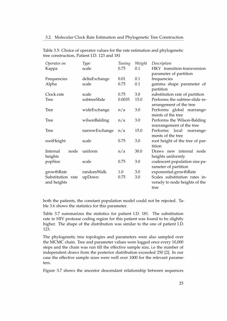
The priors specified for the BEAST run have been summarized in table 3.4.The operator setting used to explore the sample space for the parametershas been summarized in table 3.5.

23


Table 3.3: Patient I.D. 123 and 181: Analysis Settings. Results shown infig: 3.7, 3.9

Site Models Parameter1. Substitution Model HKY2. Base Frequencies Estimated3. Site Heterogeneity Model Gamma+Invariant Sites4. Partition in codon position None

Clock Model1. Model Strict Clock2 .Estimate Rate Yes

Demographic model1. Tree Prior Constant size2. Starting Tree Randomly Generated

Table 3.4: Patient I.D. 123 and 181: Priors for the BEAST run

Parameter Prior Bound DescriptionKappa Lognormal[1,1.25] [0,inf] HKY transition transversion

parameterFrequencies uniform[0,1] [0,1] base frequenciesalpha uniform[0,10] [0,1000] gammma base frequenciespInv uniform[0,1] [0,1] proportion of invariant sites

parameterclock.rate uniform[5.4E-5,1] [0,inf] substitution raterootHeight Using Tree Prior [3.761,inf] root height of the treeconst.popsize 1/x [0,inf] coalescent population size pa-

rameter

Let us now briefly discuss how the current choice of parameters was formu-lated. A series of runs were set up with parameter rich substitution modelslike general time reversible model. These initial runs took long to converge.As a result, simpler substitution model was selected for the analysis likeHKY model. This made a significant difference in the decreasing the conver-gence time of the chain. All initial test runs were made with the uncorrelatedlognormal clock which draws the rate of each branch from an underlyinglognormal distribution. The standard deviation (i.e. ucld.stdev parameter)estimate of the clock rate was close to zero for most of these runs. A valueclose to zero for this parameter indicated clock-like behavior of the dataset[2]. Thereafter a set of runs were made with different coalescent models likeexpansion growth model, exponential growth model and constant growthmodel. The Bayes Factor was used for selecting the best fitting model. For

24


Table 3.5: Choice of operator values for the rate estimation and phylogenetictree construction, Patient I.D. 123 and 181

Operates on Type Tuning Weight DescriptionKappa scale 0.75 0.1 HKY transition-transversion

parameter of partitionFrequencies deltaExchange 0.01 0.1 frequenciesAlpha scale 0.75 0.1 gamma shape parameter of

partitionClock.rate scale 0.75 3.0 substitution rate of partitionTree subtreeSlide 0.0035 15.0 Performs the subtree-slide re-

arrangement of the treeTree wideExchange n/a 3.0 Performs global rearrange-

ments of the treeTree wilsonBalding n/a 3.0 Performs the Wilson-Balding

rearrangement of the treeTree narrowExchange n/a 15.0 Performs local rearrange-

ments of the treerootHeight scale 0.75 3.0 root height of the tree of par-

titionInternal nodeheights

uniform n/a 30.0 Draws new internal nodeheights uniformly

popSize scale 0.75 3.0 coalescent population size pa-rameter of partition

growthRate randomWalk 1.0 3.0 exponential.growthRateSubstitution rateand heights

upDown 0.75 3.0 Scales substitution rates in-versely to node heights of thetree

both the patients, the constant population model could not be rejected. Ta-ble 3.6 shows the statistics for this parameter.

Table 3.7 summarizes the statistics for patient I.D. 181. The substitutionrate in HIV protease coding region for this patient was found to be slightlyhigher. The shape of the distribution was similar to the one of patient I.D.123.

The phylogenetic tree topologies and parameters were also sampled overthe MCMC chain. Tree and parameter values were logged once every 10,000steps and the chain was run till the effective sample size, i.e the number ofindependent draws from the posterior distribution exceeded 250 [2]. In ourcase the effective sample sizes were well over 1000 for the relevant parame-ters.

Figure 3.7 shows the ancestor descendant relationship between sequences

25


Table 3.6: Patient I.D. 123: Clock rate statistics

mean 1.5085E-3stderr of mean 1.922E-5median 1.4137E-3geometric mean 1.3607E-395% HPD lower 3.3823E-495% HPD upper 2.8556E-3auto-correlation time (ACT) 16204.9553effective sample size (ESS) 1261.3426

Figure 3.5: Patient I.D. 123: Substitution rate distribution. 95% confidenceinterval has been marked in blue. The red region shows the rate samplingoutside the interval

Fre

quen

cy

clock.rate

-1E-3 0 1E-3 2E-3 3E-3 4E-3 5E-30

10

20

30

40

50

60

70

80

Figure 3.6: Patient I.D. 181: Substitution rate distribution. The 95% con-fidence interval has been marked in blue. The red region shows the ratesampling outside the interval

Fre

quen

cy

clock.rate

-2.5E-3 0 2.5E-3 5E-3 7.5E-3 1E-2 1.25E-2 1.5E-2 1.75E-2 2E-20

25

50

75

100

125

150

175

26


Table 3.7: Patient I.D. 181: Clock rate statistics

mean 4.9113E-3stderr of mean 6.0229E-5median 4.4662E-3geometric mean 4.2646E-395% HPD lower 8.9876E-495% HPD upper 1.0203E-2auto-correlation time (ACT) 16264.458effective sample size (ESS) 1847.5869

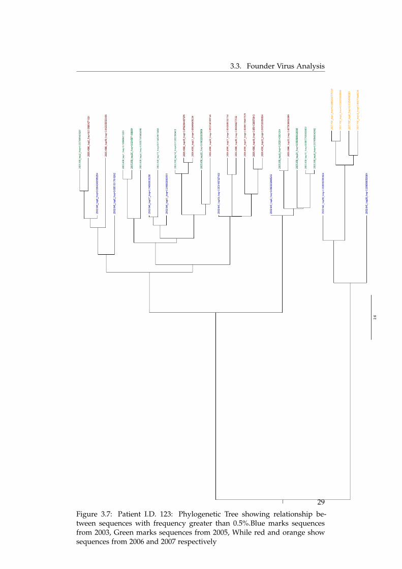
collected at different times from patient I.D. 123. Most of the sequencesfrom the first time point share nodes with the sequences from the secondand the third time point. However, the sequences from the final time point(i.e. the ones collected in 2007) appear like a segregated clade from the restof the tree showing only a faint relationship with low frequency haplotypesfrom the first time point. In a more rigorous analysis, it was found that hap-lotype number 25 (not shown in this tree as the frequency of the haplotypewas 0.02%) from the first sampling point was identical to a low frequencyhaplotype number 5 from the final time point. None of other sequences fromall the other time points were found 100% identical to any of the haplotypesfrom the final time point.

There were a series of identical haplotypes found over time. Starting fromone side of the tree, we see that haplotype 6 from 2003 branches out tohaplotype 2 of 2005 which further branches to haplotype 3 from 2006. Thesethree sequences were found to be identical over time and their frequenciesconstantly dwindled between 0.8% to 1% after which the haplotype was notvisible. There were 9 such haplotypes from the first time point that appearedagain in the later stages. These have been shown in the figure 3.8. We seein this figure that the frequency of the haplotypes decreases from the firstto the second time point but it again increases in the next time point. Thesequences from the final time point show little similarity with the ones fromprevious time points.

A pairwise sequence alignment was performed between the majority haplo-type with a frequency of 65% from the the third time point and the hap-lotype from the final time point with a frequency of 86% . These twosequences showed 97% similarity. Another tree incorporating haplotypeswith frequency as low as 0.2% was constructed to trace any relationship ofthe sequences from the final time point with low frequency variants fromthe second and the third time point. However there were no variants from2005 and 2006 sharing a node with the sequences sampled in 2007.

From a total of eight haplotypes with frequency greater than 0.5% in the first

27

3.3. Founder Virus Analysis

time point, four were found to be present in the second time point. Note thatthe second sample was collected after almost an year of the anti-retroviraltherapy. This leads us to conclude that the viral haplotypes were latentduring the therapy period but were quick to rebound when the therapy wasstopped. So, even though an year passed in terms of absolute time scalenothing much happened in terms of evolutionary time scale.

For patient I.D. 181, the haplotypes with frequency greater than 1% progres-sively increased over time. While there were only 3 haplotypes from thefirst time point with frequency greater than 1%, the number changed to 23for the final time point. All the sequences from the first time point could betraced over the three time points. The haplotype with the highest frequencyfrom the first time point remained to be the one with highest frequency overthe next two time points as well but the frequency decreased over time from87% to 38%. This can be clearly seen in figure 3.10.

3.3 Founder Virus Analysis

The analysis was carried out to detect if the infection was initiated by a singlefounder virus haplotype. This knowledge is often necessary in tracing thesource of infection. It is also useful for explaining the pattern of geneticdiversity observed in the patient. If the phylogenetic tree constructed usingsequences from only the first time point shows a star like phylogeny thenthe infection is likely to have been initiated by a single virus. When we seedistinct clades in the tree, the infection can be assumed to be initiated bymultiple founder viruses. Another reason for the phylogenetic tree to notshow a star like topology can be that the sequences are from a time wherethe immune selection already started shaping the viral evolution. Care mustbe taken to use samples that have been collected from a time very close tothe time of infection so that the intra-sample diversity is not higher than10%. When the sample shows a star like phylogeny with low intra-samplediversity, then the time of infection can be estimated using the Poisson Fittertool.

Figure 3.11 and 3.12 show the phylogenetic trees constructed using thesamples from the first time points for patient I.D. 123 and 181 respectively.These trees clearly do not show a star topology that would indicate a singlefounder virus infection. Since the exact dates of infection are unknown, itmight be the case that the samples used for the analysis were from virusesthat were evolving under selective pressure exerted by the immune system.The sample from patient 181 that was used for the analysis was collectedafter a few months of infection ( this can be seen by looking at the patient in-fection time line shown in figure 2.2), hence this result might be misleading.We see a single virus with frequency equal to 86% in the first time point. It

28


Figure 3.7: Patient I.D. 123: Phylogenetic Tree showing relationship be-tween sequences with frequency greater than 0.5%.Blue marks sequencesfrom 2003, Green marks sequences from 2005, While red and orange showsequences from 2006 and 2007 respectively

29


Figure 3.8: Patient I.D.123: Haplotypes traced over time with their measuredfrequencies

30


Figure 3.9: Patient I.D. 181: Phylogenetic Tree showing relationship betweensequences with frequency greater than 0.5%.Blue marks sequences sampledon 28.09.2005, Green marks sequences from 15.03.2006, While orange showssequences sampled on 08.09.2006

31


Figure 3.10: Patient I.D. 181: Haplotypes traced over time with their mea-sured frequencies

32


Figure 3.11: Patient I.D. 123: Phylogenetic tree with sequences from 2003with frequency greater than 0.5%

is likely that the infection was started by a single founder virus but due tothe selective immune pressure, the founder virus showed a divergent evolu-tionary pattern. Poisson Fitter analysis showed that the hamming distancedistribution of the first time point sample did not confirm with the distribu-tion expected under neutral evolution from a single founder virus. Anotherexplanation for the observation could be that the samples were not from atime point close to the initiation of infection.

Figure 3.12: Patient I.D. 181: Phylogenetic tree with sequences from 2005with frequency greater than 0.5%

33

3.4. Demographic Reconstruction

Figure 3.13: Patient I.D. 123: Demographic construction of the viral popula-tion with frequency greater than 0.5%

3.4 Demographic Reconstruction

The effective population size of the virus was plotted over the period of in-fection for patient I.D. 123 figure 3.13 and patient 181 figure 3.14. The timepoints where the sequences were collected have been marked in the plot. Wesee a slight increase in the viral population over time during course of infec-tion for patient I.D. 123. The results of this analysis were robust to the use ofdifferent model settings. This indicated that the sequence data was informa-tive and not too sensitive towards slight model mis-specification. However,since the model could not be informed about the anti-retroviral therapy pe-riod, we do not know if the results would be sensitive to this information.As previously concluded from figure 3.8 that the virus was under a latencyperiod during the therapy, one would assume that the results of the demo-graphic should not be affected by the therapy phase.

For patient I.D. 181, we see no change in the effective population size of thevirus over the first year of infection. The times of sample collection havebeen marked in the figure 3.14.

As a proof of principle of the coalescent model used in our study, anotheranalysis was performed on a sequence dataset collected over a period of3 years from an influenza epidemic. This demographic plot was in agree-ment with the variation observed during the epidemics. The data containedsequences of length 1700 base pairs and there were samples collected overevery few months giving a high coverage over a period of three years. Theresults are not shown since these are freely available on the BEAST website.

34

3.5. Sliding MinPD

Figure 3.14: Patient I.D. 181: Demographic construction of the viral popula-tion with frequency greater than 0.5%

3.5 Sliding MinPD

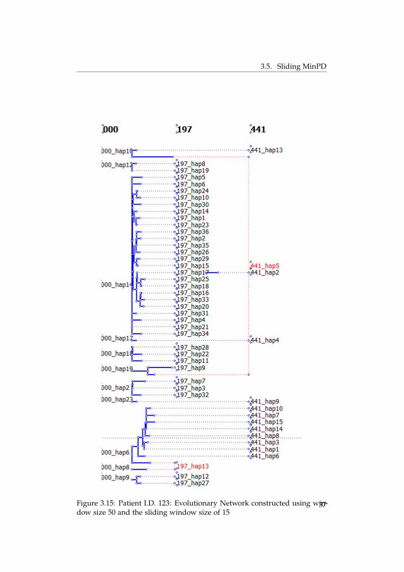
The evolutionary network was constructed for the patient I.D. 123 using theSliding MinPD software. Sequences from 2005, 2006 and 2007 were used inthe analysis. The samples from the first time point were ignored since themajority haplotypes were same between the first and the second time point.A set of runs were set up with differing window sizes and sliding windowsizes. The results of the runs were found to be sensitive to slight changes inthe window length. Due to lack of confidence in the results of this analysis,this was not carried out for patient I.D.181. The results of the run havebeen shown in figure 3.15 and 3.16. The parameters for the runs except thewindow and the sliding window size has been mentioned in table 3.8.

Table 3.8: Parameters used for constructing the evolutionary network usingSliding MinPD

Active Recombination Detection YesRecombination Detection Option Bootscan RIPCrossover option ManyPCC threshold p0.4bootstrap recomb. tiebreaker option Yesbootscan seed E-3bootscan threshold TN93substitution model 1847.5869gamma shape - rate heterogeneity alpha 0.5show bootstrap values Nomarkers for clustering Yesclustering distance threshold T0.001clustering option by bases but post

35

3.5. Sliding MinPD

In figure 3.15 and 3.16 the sequences in a single column belong to thesame time point. The ancestor descendant relationships are denoted usingblack dotted lines. The sequences marked in red are the recombinants andthe red line when traced back in time shows the two donor haplotypes.It can be clearly seen that when the window size is changed the number ofrecombinants change. Hence this analysis was not carried out for the secondpatient.

36

3.5. Sliding MinPD

Figure 3.15: Patient I.D. 123: Evolutionary Network constructed using win-dow size 50 and the sliding window size of 15

37

3.5. Sliding MinPD

Figure 3.16: Patient I.D. 123: Evolutionary Network constructed using win-dow size 50 and the sliding window size of 30

38

3.6. Conclusions

3.6 Conclusions

A series of downstream sequence analysis were carried out on the timestamped data collected from two patients. We formulated an ordered se-quence in which these standardized tests could be applied to any set of deep-sequenced, single gene datasets. These tests returned information regardingthe evolutionary pattern being followed by the virus and provided estimatesfor clinically important parameters like the time of HIV transmission andthe population structure of the virus over the infection period. While therewere no special tools used to detect the effect of anti-retroviral therapy, en-tropy measure and the change in haplotype frequency over time were usedto identify any of its visible effects. Since we used coalescent based modelsfor estimating these parameters, the estimates were unique for every patient.As this method is sensitive to the amount of genetic variation present in thedata set, the estimated parameters had large confidence intervals. The overestimation of the time of HIV transmission to the host could be attributedto the phylogenetic tree structure that did not support the single foundervirus hypothesis. This implied that the age of the root of the tree showedthe time to the common ancestor of the multiple viruses that infected thepatient rather than the time of HIV transmission to the host.

The relatively conserved protease coding sequences were successful in con-structing robust phylogenetic trees showing the relationship between thehaplotypes sequenced from samples collected at different time points. Thepre and post anti-retroviral therapy samples from the patient 123 showedhigh similarity in terms of haplotype sequences and their frequencies whichled us to conclude that the virus went under hibernation during the therapybut was quick to rebound once it was discontinued. There was no evidenceof recombination found in the sample sequences. The viral population plotswere fairly smooth indicating that the effective population size remained al-most constant over the course of infection. Even though the number of hap-lotypes with frequency greater than 1% increased over time for patient 181indicating increased intra-population diversity, this was not followed witha increase in the effective population size. A closer look at the sequenceidentity revealed that these haplotypes were on an average 99% identical.The conserved regions of the virus are able to construct stable phylogenies,but these regions should be used in combination with other variable regiondataset to provide population estimates with smaller confidence intervals.Another solution would be to increase the number of sampled time pointsfor improving the coalescent based estimates.

39

Bibliography

[1] http://www.niaid.nih.gov/factsheets/howhiv.htm.

[2] A rough guide to BEAST1.4.

[3] 61.0.6. lentivirus. International Committee on Taxonomy of Viruses, 2002.

[4] Overview of the global AIDS epidemic, 2006.

[5] D Baltimore. Viral RNA-dependent DNA Polymerase: RNA-dependentDNA polymerase in virions of RNA tumour viruses. Nature,226(5252):1209–1211, 2000.

[6] Daniel Beyer. multiplication of HIV. 1997.

[7] M T et al. Bretscher. Recombination in HIV and the evolution of drugresistance:for the better or for worse? BioEssays, 26:180–188.

[8] P. Buendia and G. Narasimhan. Sliding MinPD: Building evolutinarynetworks of serial samples via an automated recombination detectionapproach. Bioinformatics, 2007.

[9] McElroy K Gaudieri S Pham ST et al. Bull RA, Luciani F. Sequential bot-tlenecks drive viral evolution in early acute Hepatitis C Virus infection.PLoS Pathog, 7(9), 2011.

[10] Kim Pl Chan D. HIV entry and its inhibition. Cell, 93(5):681–684, 2003.

[11] Achaz G. et al. Mol Biol Evol., 21(10), 2004.

[12] Cunningham et al. Manipulation of dendritic cell function by viruses.Current opinion in microbiology, 13(4):524–529, 2010.

40

Bibliography

[13] Cynthia A. Derdeyn et al. Envelope-constrained neutralization-sensitive HIV-1 after heterosexual transmission. Science, pages 1134–1137, 2004.

[14] Drummond A. J. et al. Bayesian coalescent inference of past populationdynamics from molecular sequences. Molecular Biology and Evolution,7(214), 2007.

[15] Gilbert P B et al. Comparison of HIV-1 and HIV-2 infectivity from aprospective cohort study in senegal. Statistics in Medicine, 22(4), 2003.

[16] Giorgi EE et al. Estimating time since infection in early homogeneousHIV-1 samples using a poisson model. BMC Bioinformatics, 25(11), 2010.

[17] Korber et al. Numbering positions in HIV relative to HXB2CGl. HumanRetroviruses and AIDS, 1998.

[18] Lee et al. Modelling sequence evolution in acute HIV-1 infetion. J TheorBiol., 2009.

[19] Morgan D et al. HIV-1 infection in rural Africa: is there a difference inmedian time to AIDS and survival compared with that in industrializedcountries? AIDS, 16(4):597–632, 2002.

[20] Pond S.L. et al. Estimating selection pressures on alignments of codingsequences, 2007.

[21] Rodrigo A. et al. Mathematics of Evolution and Phylogenetics. Oxford Uni-versity Press, 2007. The Evolutionary Analysis of Measurably EvolvingPopulations using Serially Sampled gene sequences.

[22] Shankarappa et al. Consistent viral evolutionary changes associatdewith the progression of Human Immunodeficiency Virus Type 1 infec-tion. Journal of Virology, 73(12):10489–10502, 1999.

[23] Suzanne English et al. Phylogenetic analysis consistent with a clinicalhistory of sexual transmission of HIV-1 from a single donor revealstransmission of highly distinct variants. Retrovirology, 8(54), 2011.

[24] Zagordi et al. ShoRAH: Estimating the genetic diversity of a mixed sam-ple from next-generation sequencing data. BMC Bioinformatics, 12(119),2011.

[25] Zheng Y H et al. Newly identified host factors modulate HIV replica-tion. Immunol Lett, pages 225–234, 2005.

41

Bibliography

[26] Poon Art F.Y. Dates of HIV infection can be estimated for seropreva-lent patients by coalescent analysis of serial next-generation sequencingdata. AIDS, 25(16):2019–2026, 2011.

[27] Drummond A J and Rambaut A. BEAST:bayesian evolutionary analysisby sampling trees. BMC Evolutionary Biology, 7(214), 2007.

[28] H.Kishino J.L Throne. Statistical methods in molecular evolution. Springer,2005. Estimation of Divergence Times from Molecular Sequence Data.

[29] DePasquale M. P. Kartsonis N. Hanna G. J. Wong J. Finzi D. RosenbergE. Gunthard H.F. Sutton L. Savara A. Petropoulos C. J. Hellmann N.Walker B. D. Richman D. D. Siliciano R. Martinez-Picado, J. and R. T.D’Aquila. Antiretroviral resistance during successful therapy of Hu-man Immunodeficiency Virus type 1 infection. Proc. Natl. Acad. Sci. U.S. A, 97(20):10948–10953, 2000.

[30] Hall N. Advanced sequencing technologies and their wider impact inmicrobiology. J of Exp. Biol., 210(Pt 9):1518–1525, 2007.

[31] Gojobori T Nei M. Simple methods for estimating the numbers of syn-onymous and nonsynonymous nucleotide substitutions. Mol Biol Evol.,3(5), 1986.

[32] V. W. Pollard and M. H. Malim. The HIV-1 Rev protein. Annu. Rev.Microbiol., 52:491–532, 1998.

[33] Oliver G Pybus and Andrew Rambaut. Evolutionary analysis of thedynamics of viral infectious diseases. The Nature Reviews, 10:540–549,2009.

[34] Weiss RA. How does HIV cause AIDS? Science, 260(4):1273–1279, 1993.

[35] N Saitou and M Nei. The neighbor joining method:a nw method forreceonstructing phylogenetic trees. Mol Bio Evol, 4(4), 1987.

[36] Coulson AR Sanger F. A rapid method for determining sequencesin DNA by primed synthesis with DNA polymerase. J of Mol Biol,94(3):441–448, 1975.

[37] A. Siepel and B. Korber. Scanning the database for recombinant HIV-1genomes. Los Alamos National Laboratory, pages 35–60.

[38] Dan Stowell. The molecules of HIV. 2006.

42

Bibliography

[39] SM. et al. Wollinsky. Selective transmission of Human Immunodefi-ciency Virus type-1 variants from mothers to infants. Science, 255:1134–1137, 1992.

[40] Sodroski J Wyatt R. The HIV-1 envelope glycoproteins: fusogens, anti-gens, and immunogens. Science, 280(5371):1884–8, 1998.

[41] Ziheng Yang. Computational Molecular Evolution. Oxford, 2006.

43

phylogenetic analysis of hiv samples from a single host

Documents