LUND UNIVERSITY

PO Box 117221 00 Lund+46 46-222 00 00

Physical bounds and sum rules for high-impedance surfaces

Gustafsson, Mats; Sjöberg, Daniel

2010

Link to publication

Citation for published version (APA):Gustafsson, M., & Sjöberg, D. (2010). Physical bounds and sum rules for high-impedance surfaces. (TechnicalReport LUTEDX/(TEAT-7198)/1-17/(2010); Vol. TEAT-7198). [Publisher information missing].

Total number of authors:2

General rightsUnless other specific re-use rights are stated the following general rights apply:Copyright and moral rights for the publications made accessible in the public portal are retained by the authorsand/or other copyright owners and it is a condition of accessing publications that users recognise and abide by thelegal requirements associated with these rights. • Users may download and print one copy of any publication from the public portal for the purpose of private studyor research. • You may not further distribute the material or use it for any profit-making activity or commercial gain • You may freely distribute the URL identifying the publication in the public portal

Read more about Creative commons licenses: https://creativecommons.org/licenses/Take down policyIf you believe that this document breaches copyright please contact us providing details, and we will removeaccess to the work immediately and investigate your claim.

Electromagnetic TheoryDepartment of Electrical and Information TechnologyLund UniversitySweden

CODEN:LUTEDX/(TEAT-7198)/1-19/(2010)

Revision No. 1: October 2010

Physical bounds and sum rules forhigh-impedance surfaces

Mats Gustafsson and Daniel Sjoberg

Mats Gustafsson and Daniel SjöbergMats.Gustafsson@eit.lth.se, Daniel.Sjoberg@eit.lth.se

Department of Electrical and Information TechnologyElectromagnetic TheoryLund UniversityP.O. Box 118SE-221 00 LundSweden

Editor: Gerhard Kristenssonc© Mats Gustafsson and Daniel Sjöberg, Lund, October 21, 2010

1

Abstract

High-impedance surfaces are articial surfaces synthesized from periodic struc-

tures. The high impedance is useful as it does not short circuit electric currents

and reects electric elds without phase shift. Here, a sum rule is presented

that relates frequency intervals having high impedance with the thickness of

the structure. The sum rule is used to derive physical bounds on the band-

width for high-impedance surfaces composed by periodic structures above a

perfectly conducting ground plane. Numerical examples are used to illustrate

the result, and show that the physical bounds are tight.

1 Introduction

A perfect magnetic conductor (PMC) surface is an ideal high-impedance surface.It has innite impedance meaning that the mirror currents of horizontal electricalcurrents are not phase shifted. This is desired for low prole antennas as ordi-nary planar antenna elements can be put on top of a PMC without loss of per-formance [20, 21]. However, PMCs are articial surfaces typically synthesized fromperiodic structures above an ordinary ground plane [2022]. The properties of thearticial high-impedance surface depend on frequency, polarization, and angle ofincidence, and they have high impedance only over nite frequency bands [20, 21].

Here, we introduce a sum rule that relates frequency intervals having impedanceabove an arbitrary threshold with the static properties of the structure. The sumrule is valid for periodic structures composed by arbitrary dielectric and magneticmaterials above a perfect conductor. The sum rule is used to derive physical boundsfor high-impedance surfaces. The bounds show how the bandwidth of the high-impedance surface depends on thickness, angle of incidence, polarization, and ma-terial properties. The derivation is based on a general approach where integralidentities for positive real (PR) functions (or similarly Herglotz functions) are usedto construct sum rules [1]. Analogous bounds are used for broadband matching [4],radar absorbers [18], scattering and absorption cross sections [25], antenna per-formance [9], antenna impedance [6], extraordinary transmission [10], transmissionblockages [11], and temporal dispersion of metamaterials [8].

Brewitt-Taylor presented two bounds for high-impedance surfaces in [2]. The rstis based on circuit approximation whereas the second is similar to [18]. Anothercontribution is given in [19], although their result is based on an approximationthat may break down for large bandwidths. In comparison, the results presentedhere are solely based on passivity and make no use of circuit approximations. Thenew bounds are also sharper than the bounds presented in [2]. Moreover, theyhold for lossy as well as lossless surfaces (including possible anisotropy) and forobliquely incident elds. Finally, they are based on an identity and it shows thatobjects modeled as perfect electric conductors contribute with a negative magneticpolarizability that can aect the performance.

This paper is organized as follows. In Sec. 2, the reection coecient and theimpedance of periodic high-impedance surfaces are presented. The corresponding

2

d

`

`x

y

E (r)E

z

x

yz=0

z=-d

(i)

Figure 1: Geometry of a high-impedance surface synthesized by a periodic structureabove a perfect conductor.

low-frequency asymptotics are analyzed in Sec. 3. Sum rules and physical boundsare derived in Sec. 4. The bounds are compared with previous results in Sec. 5.Numerical results are presented in Sec. 6.

2 Reection coecient and impedance

Consider an innite array contained in the interval −d ≤ z ≤ 0, with a unit cell Ωlying in the xy-plane and a ground plane at z = −d, see Fig. 1. A linearly polarizedplane wave impinges on the array in the direction k, i.e., E(i)(t; r) = E0(t−k·r/c0)ewith k · z < 0 and E0(t′) = 0 for t′ < 0. Here, t′ = t − k · r/c0, where t is thetime variable, c0 the speed of light in free space, and e the electric polarization ofthe incident eld satisfying e · k = 0. The periodicity of the problem implies thetranslational property

E(t; r + rmn) = E(t− k · rmn/c0; r) (2.1)

for all elds, where rmn = ma1 + na2 is an arbitrary lattice vector described bytwo basis vectors a1 and a2. The reected eld cannot precede the incident eld inz > 0, in the meaning that E(r)(t; r) = 0 if t < k(r) · r/c0, where k

(r) = k − 2k · zzis the mirrored propagation direction. In other words, the reected eld is causalfor all z > 0 with respect to the incident eld, see also [7, 11, 25, 26].

The results in this paper follow from the holomorphic properties of the reectioncoecient and its low- and high-frequency expansions. For this purpose, apply atemporal Laplace transform to the reected eld taking the causality into accountby the lower integration limit, i.e.,

E(r)(κ; r) =

∫ ∞k(r)·r/c0

E(r)(t; r)e−κtc0 dt

= e−κk(r)·r∫ ∞

0

E(r)(t′ + k(r)· r/c0; r)e−κt

′c0 dt′ = e−κk(r)·rE(r)(κ; r). (2.2)

3

The eld E(r)(κ; r) is Ω-periodic in r due to the translational property (2.1) andthat k(r) has the same xy-components as k. The lower integration limit t′ = 0 forE(r)(κ; r) implies it is holomorphic in the Laplace parameter κ = σ + jk if thisis restricted to the right complex half plane Reκ ≥ 0, and the imaginary unit isdenoted by j. A spectral decomposition in Floquet modes is used outside the array(where the position vector is r = xx+ yy + zz = ρ+ zz):

E(r)(κ; r) =∞∑

m,n=−∞

E(r)mn(k)e−jkmn·ρe−j(kz,mn−kz,00)z, (2.3)

where the expansion coecients are given by

E(r)mn(κ) =

1

A

∫Ω

E(r)(k; r)ejkmn·ρej(kz,mn−kz,00)z dSρ. (2.4)

Here, A =∫

ΩdS denotes the area of the unit cell Ω. The reciprocal lattice vectors

are dened as kmn = mb1 +nb2, where the reciprocal basis vectors b1 and b2 satisfyai · bj = 2πδij for i, j = 1, 2 (δij is the Kronecker delta) [14]. Moreover, the wave

number in the z-direction is given by k2z,mn = −κ2 + (κkt + jkmn) · (κkt + jkmn),

where kt is the transverse part of the unit vector k. The transverse componentsof the expansion coecients of the reected eld are related to the correspondingexpansion coecients of the incident eld via the linear mapping

E(r)mn,t(κ) =

∞∑m′,n′=−∞

Γmn,m′n′(κ) ·E(i)m′n′,t(κ). (2.5)

The corresponding z-components are given by the requirement that each mode E(i,r)mn

is orthogonal to the total wave vector −jκkt + kmn ± zkz,mn. The elements of the2 × 2 reection dyadics Γmn,m′n′ , are holomorphic functions of κ for Reκ > 0 dueto causality. It is only a nite number of modes in (2.5) that propagate for a xedfrequency, and, specically, it is only the lowest order modes (m = n = m′ = n′ = 0)that propagate for frequencies below the rst grating lobe [17]. Here, the analysisis restricted to these modes, and the short-hand notation Γ = et · Γ 00,00 · et/|et|2for the co-polarized reection coecient is introduced. These are the only modesneeded later on, without loss of generality.

Passivity implies that |Γ (κ)| ≤ 1 for Reκ > 0. The corresponding normalizedimpedance

Z(κ) = Zt1 + Γ (κ)

1− Γ (κ)(2.6)

is then a positive real function [5, 28]. The impedance in (2.6) is normalized withrespect to the transverse wave impedance Zt(θ) = 1/Yt(θ), where

Yt(θ) =

cos θ TE-polarization

1/ cos θ TM-polarization(2.7)

4

is the transverse wave admittance. The impedance in SI-units is ZSI = Zη0, whereη0 =

√µ0/ε0 ≈ 377 Ω denotes the free-space impedance.

Positive real (related to Herglotz [1] or Nevanlinna) functions are found in theanalysis of passive linear systems [5, 28]. They are dened as holomorphic mappingsfrom the right complex half plane into itself and having the real axis mapped intoitself. Sum rules, i.e., weighted all spectrum integral identities, are solely determinedfrom the asymptotic expansions of the PR function. In [1], it is shown that theasymptotic expansions

P (κ) =

N0∑n=0

a2n−1κ2n−1 + o(κ2N0−1) as κ→0 (2.8)

and

P (κ) =N∞∑n=0

b1−2nκ1−2n + o(κ1−2N∞) as κ→∞ (2.9)

imply the integral identities

2

π

∫ ∞0

ReP (jk)

k2ndk = (−1)n−1

(a2n−1 − b2n−1

)(2.10)

for n = 1 − N∞, ..., N0. Note that the identity (2.10) should be interpreted as thelimit limσ→0+ P (σ+jk), and terms in the right hand side that are not enumerated in(2.8) and (2.9) are zero, see [1]. It is sucient to have the expansions (2.8) and (2.9)in | arg(κ)| ≤ π/2 − α for some α > 0. It is observed that compositions of PRfunctions can be used to produce new PR functions and hence sum rules that areparticularly suited for an application [1, 8].

3 Low-frequency expansion

3.1 Reection coecient

The integral identities (2.10) show that the low- and high-frequency asymptoticexpansions can be used to derive constraints on the dynamic properties of theimpedance. To determine the low-frequency expansion of the reection coecient,we rst replace the ground plane with a mirror object in the region z ∈ [−2d,−d],see Fig. 2. The reected eld is obtained from superposition of the incident eldand the mirror eld, i.e.,

E(i)(κ, r) = E0e exp(−κk · r) (3.1)

E(i)m (κ, r) = E0e

(r) exp(−κk(r) · (r + 2dz)) (3.2)

where k(r) = k − 2k · zz and e(r) = 2e · zz − e. The reected eld E(r)(κ, r) isobtained as the sum of the reection of E(i)(κ, r) and the transmission of E(i)

m (κ, r)in the mirrored geometry in Fig. 2b. Using the low-frequency expansion in [23]

5

PEC

z z

²(x,y,z)

²(x,y,-z)

¹(x,y,z)²(x,y,z)

¹(x,y,z)

¹(x,y,-z)

k

e

^

e

k

ke

a) b)

(r)

0

-d

-2d(r)

Figure 2: Equivalent problem for the low-frequency expansion. a) original scat-tering problem with ground plane. b) equivalent scattering problem without theground plane, where k(r) = k − 2k · zz and e(r) = 2e · zz − e.

and that E(i)m (κ, r)|z=0 = E0e

(r)(1 − 2κd cos θ), we derive in the Appendix that theco-polarized reection coecient is, to rst order in κ,

Γ (κ) = −1 + κ(2d cos θ + γ/A

)+O(κ2), (3.3)

where the polarizability γ is

γ =

h · γm · h cos θ TE

h · (γm + sin2 θγeI) · h 1cos θ

TM(3.4)

and the unit vector h = (z× e)/|z× e| corresponds to the direction of the incidentmagnetic eld in the xy-plane. The magnetic polarizability dyadic γm is determinedin the unit cell Ω subject to periodic boundary conditions in the xy-plane anda magnetostatic eld of unit amplitude in the h-direction. More precisely, themagnetic polarizability is dened as

h · γm · h = h ·∫

Ω×[−2d,0]

(µs(r)− I) ·Hs(r) dV, (3.5)

where the static eld Hs(r) satises the dierential equations ∇ × Hs(r) = 0and ∇ · [µs(r) ·Hs(r)] = 0, with mean value h in Ω × (−∞,∞), or, equivalently,limit values Hs(r)→ h as z → ±∞. Here, µs(r) is the static relative permeabilitydyadic. We can correspondingly compute an electric polarizability dyadic γe, simplyreplace µs by εs. The normal electric polarizability γe (a scalar, denoted by γezz inthe Appendix for clarity) is then computed as

γe = z · γe · z = z ·∫

Ω×[−2d,0]

(εs(r)− I) ·Es(r) dV, (3.6)

where Es(r) is the electrostatic solution corresponding to unit excitation in the zdirection. For more details on the computation of γm and γe, in particular wheninvolving PEC structures (where µs → 0 and εs →∞), we refer to [23, 24].

6

3.2 Examples of polarizabilities

The polarizabilities for an isotropic slab (with thickness 2d corresponding to themirrored geometry in Fig. 2) characterized by static relative permeability µs andstatic relative permittivity εs are

γm = 2Ad(µs − 1)(xx+ yy) + 2Ad(1− µ−1s )zz (3.7)

γe = 2Ad(εs − 1)(xx+ yy) + 2Ad(1− ε−1s )zz. (3.8)

Using these expressions, we nd that (3.4) becomes (using that for TM polarizationwe can write γ/A = 2d(µs − 1 + sin2 θ(1− ε−1

s )) = 2d(µs − ε−1s sin2 θ − cos2 θ))

2d cos θ + γ/A =

2dµs cos θ TE

2dµs−ε−1s sin2 θcos θ

TM.(3.9)

For normal incidence (θ = 0) we then see that (3.3) becomes

Γ (κ) = −1 + κµs2d+O(κ2) (3.10)

for both polarizations, which is the familiar result used in [18].In addition to variations in permittivity and permeability, objects that are mod-

eled as perfect electric conductors (PEC) also give a contribution to the polarizabil-ity, in particular γm. These objects can be considered as having static permeabilityµr(0) = 0 and hence have a negative semi-denite γm, e.g., a PEC sphere with radiusa has γm = −2πa3I. There are a few other shapes with simple expressions for γm

such as spheroids [3]. For a general geometry the polarizabilities can be calculatednumerically [15].

Thin patches modeled as PEC are particularly common for high-impedance sur-faces [20], see the examples in Sec. 6. They have polarizability dyadics of the form

γm = γzzzz and γe = γtt(xx+ yy), (3.11)

where it is observed that they do not contribute to the low-frequency expansion (3.3).They can however contribute when they are connected to the ground plane with avia. This contribution is analyzed numerically in Sec. 6 but it can also be estimatedfrom the transverse magnetic polarizability of an innite PEC cylinder of radius athat has

γm = −2πa2`z(xx+ yy) (3.12)

per unit length `z. The electric polarizability along the cylinder grows approximatelyas `3

z, and is increased when the cylinder is terminated by a patch, whereas the mag-netic transverse polarizability does not change much by the addition of the patch.The addition of patches improves the approximation of the magnetic polarizabilityby the innite cylinder, since the boundary condition n ·H = 0 helps keeping themagnetic eld in the xy-plane and reduces the fringe eld.

Variational results for static problems state that the polarizability dyadics γm

and γe are monotone in µs and εs, in the respect that if µs (or εs) is increased

7

-1.5 -1 -0.5 0 0.5 1 1.5 2

-2

-1.5

-1

-0.5

0

0.5

1

1.5

2

Re P (j!)¢

Im P (j!)¢

P (j!)¢

!/¢

Figure 3: The PR pulse function P∆(jω) in (4.3).

anywhere in Ω × [−2d, 0], then the quadratic form h · γm · h (or z · γe · z) doesnot decrease [12, 24]. This means that γm can be estimated by rst increasing µs

everywhere up to its maximum value maxr h ·µs · h = µmaxs . The resulting structure

is a homogeneous slab with transverse polarizability 2Ad(µmaxs − 1) according to

(3.7), which is an upper bound to h · γm · h. The normal electric polarizability isestimated by letting εs →∞ in (3.8), which implies γe ≤ 2Ad. Our nal estimate isthen

2d cos θ + γ/A ≤ 2dµmaxs Yt(θ), (3.13)

where Yt(θ) is the normalized transverse wave admittance in free space (2.7). Thisestimate is valid regardless of how the structure is realized, i.e., this bound appliesto any structure with thickness d backed by a ground plane, including anisotropicmaterials and PEC structures.

4 Sum rules and physical bounds

The normalized impedance (2.6) has the low-frequency expansion

Z(κ)

Zt(θ)=

1 + Γ (κ)

1− Γ (κ)= κ(d cos θ + γ/(2A)) +O(κ2) (4.1)

as κ→0. We are interested in regions with Γ ≈ 1 or equivalently |Z| ≥ ∆−1 where0 < ∆ < 1 is a number used to quantify the high-impedance surface. It is alsoconvenient to consider the normalized admittance Y = 1/Z that has |Y | ≤ ∆ forhigh impedance surfaces. The admittance has the asymptotic expansions

Y (κ) =

Yt(θ)

κ(d cos θ+γ/(2A))+ o(κ−1) as κ→0

κα as κ→∞,(4.2)

where α ≥ 0. The constant α is in general unknown but it is known that thehigh-frequency asymptotic is at most linear for PR functions [28].

8

To relate the intervals with |Y (k)| ≤ ∆ with the low-frequency asymptotic ex-pansion (4.2), we consider the composition of Y with

P∆(s) =1

π

∫ ∆

−∆

s

ξ2 + s2dξ =

1

jπln

js−∆js+∆

. (4.3)

that can be extended to the imaginary axis except for s = ±j∆, see Fig. 3. This isa positive real function with the properties [8]

ReP∆(s) ≤ 1 for all s

ReP∆(s) ≥ 1/2 for |s| < ∆

ReP∆(s) = 1 for |s| < ∆ and Re s = 0

ReP∆(s) = 0 for |s| > ∆ and Re s = 0

(4.4)

it is hence well suited to bound regions with low admittance. The compositionP∆(Y ) denes a positive real function with the asymptotic expansions

P∆(Y (κ)) =

2κ(d cos θ+γ/(2A))∆

πYt(θ)+ o(κ) as κ→0

o(κ) as κ→∞.(4.5)

The integral identities for PR function (2.10) gives the n = 1 sum rule∫ ∞0

ReP∆(Y (jk))

k2dk =

(d cos θ +

γ

2A

) ∆

Yt(θ). (4.6)

Note the sum rule only depends on the low frequency limit due to the o(κ) highfrequency dependence of P∆(Y (κ)). It is convenient to rewrite it into∫ ∞

0

ReP∆(Y (λ)) dλ =(d cos θ +

γ

2A

) 2π∆

Yt(θ), (4.7)

where λ = 2π/k denotes the wavelength and the symbol Y is reused to denote theadmittance as function of the wavelength.

Use that the integrand is non-negative to bound (4.7) as

Bminλ∈B

ReP∆(Y (λ)) ≤ 1

λ0

∫ λ2

λ1

ReP∆(Y (λ)) dλ ≤2π(d cos θ + γ

2A

)∆

λ0Yt(θ), (4.8)

where B = [λ1, λ2], λ0 = (λ1+λ2)/2 is the center wavelength and B = (λ2−λ1)/λ0 isthe fractional bandwidth. The properties (4.4) show that minλ∈B ReP∆(Y (λ)) ≥ 1/2for maxλ∈B |Y (λ)| = ∆ and minλ∈B ReP∆(Y (λ)) ≥ 1 if in addition maxλ∈B ReY (λ) =0. Normalizing with λ0/d, this gives the bound

Bλ0

d≤ 4π

Yt(θ)

(cos θ +

γ

2Ad

)maxλ∈B|Y (λ)|

1 lossy case12

lossless case(4.9)

9

which is our main result. The variational bound (3.13) can be used to give

Bλ0

d≤ 4πµmax

s maxλ∈B|Y (λ)|

1 lossy case

1/2 lossless case.(4.10)

This version of the bound is independent of the specic realization of the highimpedance surface, whereas (4.9) is sharper if the polarizability γ can be com-puted. A common case is when the high-impedance surface is realized by loss-less, non-magnetic materials and operating below the rst grating lobe. Allowingmaxλ∈B |Y (λ)| = 1/2, the normalized bandwidth is bounded by

Bλ0

d≤ π. (4.11)

In terms of the wavenumber, this becomes B ≤ k0d/2. Note that (4.10) and (4.11)are independent of the angle of incidence.

5 Comparison with previous bounds

The new bound (4.10) is sharper than the bounds presented in [2, 19]. The boundsin [2] are for lossless structures and expressed in the fractional bandwidth B forphase interval Φ, i.e., the reection has the phase shift |φ| ≤ Φ/2. The ideal highimpedance surface has φ = 0. The reection coecient has unit amplitude forlossless structures and can be written Γ = e−jφ. The corresponding admittance isYlossless = −j tan(φ/2) with maximum amplitude tan(Φ/4) if Φ < 2π, giving thebound

Bλ0

d≤ 2π tan(Φ/4) ≈

π2Φ, Φ 1

2π, Φ = π

2.6, Φ = π/2

(5.1)

for normally incident waves. Brewitt-Taylor [2] has

Bλ0

d≤ πΦ and

Bλ0

d≤ π2

ln(2/Φ). (5.2)

The rst bound is based on a circuit approximation whereas the second uses Cauchyintegrals as in [18]. It is noted that the new bound (5.1) is sharper than the boundsin (5.2). The bound in [19] is based on a transmission line model for a frequencyselective surface above a ground plane. For a vacuum layer it gives

Bλ0

d≤ πΦ sin2(kd)

(kd)2≈ πΦ for kd 1 (5.3)

which is similar to (5.2). Once again, the bound (5.1) is tighter.

10

6 Numerical examples

6.1 Dielectric slab

The reection coecient for a normally incident wave on a dielectric slab above aground plane is

Γ (κ) =Γ0 − e−2κnd

1− Γ0e−2κnd, (6.1)

where κ = jk + σ, Γ0 = (η − η0)/(η + η0), κn =√κ2εr, and η = 1/

√ε. It has the

low frequency expansion

Γ = −1 + 2κd+O(κ2), as κ→ 0. (6.2)

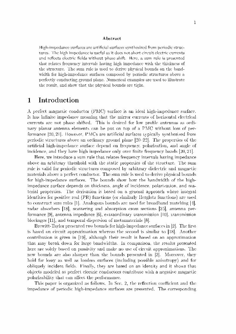
As an example, consider the reection determined in free space at the distance dfrom a ground plane, i.e., εs = 1 in the equations above. The admittance is innitefor d/λ = kd/(2π) = n/2 and vanishes for d/λ = 1/4 + n/2, where n = 0, 1, 2, ...,see Fig. 4. The structure is lossless so the admittance is purely imaginary whereit is dened. This means that ReY (k) = 0 except at the singular points. Thecomposition P∆(Y (k)) is determined for ∆ = 1/2, and it is noted that P∆(Y (k)) = 1for wavenumbers such that |Y (k)| < ∆ = 1/2.

The sum rule (4.7) shows that the area under the curve ReP∆(Y ) in Fig. 4b is2π∆ = π. This is also conrmed by numerical integration. The physical bound (4.10)can hence be interpreted as a bound on the area under the curve around the res-onance wavelength λ0. It is found that B ≈ 59% and Bλ0/d ≈ 2.6. This meansthat the design is B/Bbound ≈ 2.6/π ≈ 82% relative an optimal design. The opti-mal design must have negligible contributions to the area in (4.7) from wavelengthsoutside the desired resonance.

An increased permittivity, εr, in the dielectric layer reduces the thickness of thehigh impedance surface. The functions ReP∆(Y ) and ImY are depicted in Fig. 5for εr = 4. The bandwidth is determined to B ≈ 31% that is compared to thebound Bbound ≈ 38%. Note that B/Bbound ≈ 82% and Bλ0/d ≈ 2.6 are similar tothe εr = 1 case in Fig. 4.

6.2 Mushroom surface

The mushroom structure [20] is one of the most common structures in high impedancesurfaces. The structure used here consists of rectangular patches with widths wx =wy = w connected to a ground plane by a cylinder with height d = 8 mm and ra-dius a = 1 mm. The elements are arranged in a rectangular periodic structure withinter-element spacing ` = 10 mm, see Fig. 6. The simulations were made for aninnite PEC periodic structure using the F-solver in the commercial program CSTMicrowave Studio.

The normalized admittance Y and the composition P∆(Y ) are depicted in Fig. 7as a function of the wavelength for the case w = 8 mm. The rst grating lobe is atλ/d = 5/4 meaning that the admittance is purely imaginary for longer wavelengths.It is observed that the admittance Y ≈ 0 for λ/d ≈ 6.9. In particular it is found that

11

-2

-1

0

1

2

-2

-1

0

1

2

¸/d

Im Y

Re P (Y )¢

¢

-¢

¢

-¢

Im Y

Re P (Y )¢

a)

b)

2.6

kd

d² =1r

2¼ 3¼¼/2 ¼ 3¼/2 5¼/2

2 4 6 8 10 12

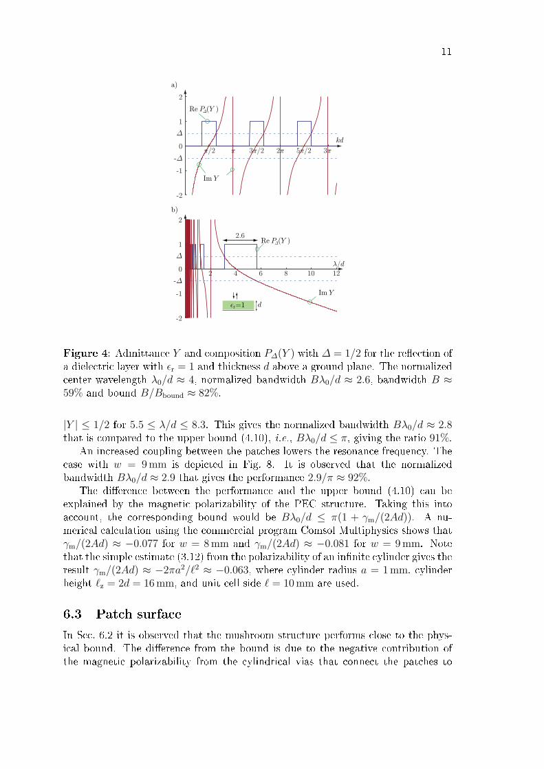
Figure 4: Admittance Y and composition P∆(Y ) with ∆ = 1/2 for the reection ofa dielectric layer with εr = 1 and thickness d above a ground plane. The normalizedcenter wavelength λ0/d ≈ 4, normalized bandwidth Bλ0/d ≈ 2.6, bandwidth B ≈59% and bound B/Bbound ≈ 82%.

|Y | ≤ 1/2 for 5.5 ≤ λ/d ≤ 8.3. This gives the normalized bandwidth Bλ0/d ≈ 2.8that is compared to the upper bound (4.10), i.e., Bλ0/d ≤ π, giving the ratio 91%.

An increased coupling between the patches lowers the resonance frequency. Thecase with w = 9 mm is depicted in Fig. 8. It is observed that the normalizedbandwidth Bλ0/d ≈ 2.9 that gives the performance 2.9/π ≈ 92%.

The dierence between the performance and the upper bound (4.10) can beexplained by the magnetic polarizability of the PEC structure. Taking this intoaccount, the corresponding bound would be Bλ0/d ≤ π(1 + γm/(2Ad)). A nu-merical calculation using the commercial program Comsol Multiphysics shows thatγm/(2Ad) ≈ −0.077 for w = 8 mm and γm/(2Ad) ≈ −0.081 for w = 9 mm. Notethat the simple estimate (3.12) from the polarizability of an innite cylinder gives theresult γm/(2Ad) ≈ −2πa2/`2 ≈ −0.063, where cylinder radius a = 1 mm, cylinderheight `z = 2d = 16 mm, and unit cell side ` = 10 mm are used.

6.3 Patch surface

In Sec. 6.2 it is observed that the mushroom structure performs close to the phys-ical bound. The dierence from the bound is due to the negative contribution ofthe magnetic polarizability from the cylindrical vias that connect the patches to

12

-2

-1

0

1

2

¸/d

Im Y

Re P (Y)¢

¢

-¢

2.6

d² =4r

2 4 6 8 10 12

Figure 5: Admittance function Y and composition P∆(Y ) with ∆ = 1/2 for thereection of a dielectric slab with εr = 4 and thickness d above a ground plane.The normalized center wavelength λ0/d ≈ 8, normalized bandwidth Bλ0/2 ≈ 2.6,bandwidth B ≈ 31% and bound B/Bbound ≈ 82%.

d

`

w

w

`x

x

y

y

Figure 6: Geometry of the mushroom structure: height d, unit cell ` = `x = `y,and patch width w = wx = wy.

the ground plane. In the patch surface the vias are removed from the mushroomstructure. This creates a structure that should perform close to the physical bound.Note, that the vias are essential for the stop band of the surface wave [13, 20, 21].

The patch structure in Fig. 9 with w = 9 mm has the normalized bandwidthBλ0/d ≈ 3.1 that gives the performance B/Bbound ≈ 98%. This conrms that themagnetic polarizability of the PEC vias reduce the performance for the mushroomstructure. The performance of the patch structure is further improved with widerpatches. The case with w = 9.9 mm gives e.g., λ0/d ≈ 10.6, and the normalizedbandwidth Bλ0/d ≈ 3.12 with the performance B/Bbound ≈ 99%.

6.4 Oblique incidence

The high-impedance surfaces composed by the dielectric slabs in Sec. 6.1, the mush-room structure in Sec. 6.2 with width w = 0.9 `, and the patch structure in Sec. 6.3with the width w = 0.9` are used to illustrate the bandwidth performance foroblique angles of incidence. CST Microwave studio was used to determine the re-ection coecients in the TE- and TM polarizations for θ ≤ 80. The performance

13

-2

-1.5

-1

-0.5

0

0.5

1

1.5

2

2 4 6 8 10 12

2.8

¸/d

¢

-¢

Im Y

Re P (Y)¢

d=0.8`

`

w=0.8`

Figure 7: Normalized admittance Y and composition P∆(Y ) with ∆ = 1/2 for amushroom structure with ` = 10 mm, w = 8 mm, and d = 8 mm. The normalizedcenter wavelength λ0/d ≈ 6.9, normalized bandwidth Bλ0/d ≈ 2.8, bandwidthB ≈ 41% and bound B/Bbound ≈ 91%.

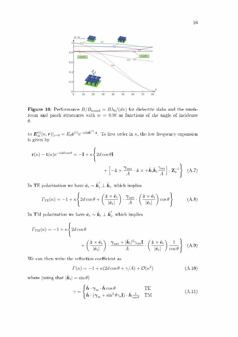
B/Bbound = Bλ0/(dπ) is depicted in Fig. 10. It is noted that the performance ofthe patch surface deteriorates for large angles of incidence whereas the mushroomstructure performs well, i.e., close to 90%, for all angles of incidence. The perfor-mance for the mushroom structure can also be improved by removing the negativemagnetic permeability by reducing the radius of the via.

6.5 Aperture surface

Aperture surfaces oer an alternative design for high-impedance surfaces [16]. Theyare composed of a perforated conducting structure above a ground plane. We use theaperture surface depicted in Fig. 11 to illustrate the sum rule (4.6) and bound (4.10).

The sum rule is evaluated for the metallic part modeled as PEC and with theconductivities σ = 105 S/m and σ = 106 S/m. For the nite conductivities, numeri-cal integration of CST data give values close to dπ for ∆ = 1/2, whereas the PECintegral only gives 0.18dπ. It is observed that the integrand in (4.6) approaches thePEC case for kd > δ for any δ > 0 as σ →∞, see Fig. 11. However, the integrandalso has large contributions from the region kd ≈ 0 that are not present in the PECcase. The signicantly smaller integral for the PEC is due to the extra negative mag-netic polarizability for a connected PEC sheet above a ground plane as discussed atthe end of the Appendix. This contribution is absent for nite conductivity.

Conclusions

Performance bounds are important as they indicate what is impossible and whatmight be possible. They also show tradeos between dierent design parameters.Here, a general approach for deriving sum rules and physical bounds on passivesystems is utilized to analyze high-impedance surfaces. The bounds show that the

14

-2

-1.5

-1

-0.5

0

0.5

1

1.5

2

2 4 6 8 10 12

2.9

¸/d

¢

-¢

Im Y

Re P (Y)¢

d=0.8`

`

w=0.9`

Figure 8: Normalized admittance Y and composition P∆(Y ) with ∆ = 1/2 for amushroom structure with ` = 10 mm, w = 9 mm, and d = 8 mm. The normalizedcenter wavelength λ0/d ≈ 8.4, normalized bandwidth Bλ0/d ≈ 2.9, bandwidthB = 34% and bound B/Bbound ≈ 92%.

bandwidth depends on the thickness and the static permeability for normally inci-dent waves. There is also a contribution from the polarizability dyadics for obliqueangles of incidence and material structures modeled as PEC.

7 Acknowledgement

The authors gratefully acknowledges the nancial support of the Swedish ResearchCouncil (VR), the Swedish Foundation of Strategic Research (SSF), and the SwedishDefence Materiel Administration (FMV).

Appendix A Low-frequency expansion

In this appendix, we calculate the low frequency reection from a general structurewith a ground plane as in Fig. 1. By using the mirror eld as described in Fig. 2,the transverse reected eld can be expressed as (where index t denotes transversecomponents)

E(r)t (κ, r) =

(r ·E(i)

t (κ, r) + t ·E(i)m,t(κ, r)

)|z=0e−κk

(r)·r (A.1)

The matrices r and t are the transverse reection and transmission matrices for alow-pass structure (without a ground plane, corresponding to Fig. 2b) as describedin [23]. The mirror symmetry in Fig. 2 implies that an exciting eld in the z directioncan not cause a total electric or magnetic dipole moment in the transverse direction,and vice versa. The low-frequency expansions in [23] of these matrices are then (upto rst order in κ, where kt is the transverse part of the propagation direction k

15

0

2 4 6 8 10 12

-2

-1.5

-1

-0.5

0

0.5

1

1.5

2

3.1

¸/d

¢

-¢

Im Y Re P (Y)¢

d=0.8`

`

w=0.9`

Figure 9: Normalized admittance Y and composition P∆(Y ) with ∆ = 1/2 for apatch structure with ` = 10 mm, w = 9 mm, and d = 8 mm. The normalized centerwavelength λ0/d ≈ 8.6, normalized bandwidth Bλ0/d ≈ 3.1, bandwidth B ≈ 36%and bound B/Bbound ≈ 98%.

and k′t = z × kt)

r(κ) = −κ2

Z0 ·

[γett

A+ k

′tk′t

γmzz

A

]−[−z × γmtt

A· z ×+ktkt

γezz

A

]· Z−1

0

(A.2)

and

t(κ) = I− κ

2

Z0 ·

[γett

A+ k

′tk′t

γmzz

A

]+[−z × γmtt

A· z ×+ktkt

γezz

A

]·Z−1

0

(A.3)

The normalized wave impedance dyadic in free space is

Z0 = cos θktkt

|kt|2+

1

cos θ

k′tk′t

|kt|2(A.4)

The electric and magnetic polarizability matrices γe and γm are dened by theinduced electric and magnetic dipole moments p = ε0γe ·E0 and m = γm ·H0 forapplied static eldsE0 andH0. They are decomposed in transverse and longitudinalparts as

γe = γett + γetzz + zγezt + γezzzz (A.5)

The dyadic γett has only transverse components and can be represented as a 2 ×2 matrix, γetz and γezt are vectors in the transverse plane, and γezz is a scalar.Corresponding expressions apply for γm. The co-polarized reection coecient Γ (κ)is then

Γ (κ) =et · r(κ) · et + et · t(κ) · e(r)

t e−κ2d cos θ

|et|2(A.6)

where et is the transverse part (xy-components) of the polarization vector e, with

the mirror polarization satisfying e(r)t = −et. The exponential factor e−κ2d cos θ is due

16

0 10 20 30 40 50 60 70 800

0.2

0.4

0.6

0.8

1

µ

² =4r² =1r

TM

TE

TM

TE

µ

B/Bbound

Figure 10: Performance B/Bbound = Bλ0/(dπ) for dielectric slabs and the mush-room and patch structures with w = 0.9` as functions of the angle of incidenceθ.

to E(i)m (κ, r)|z=0 = E0e

(r)e−κ2dk(r)·z. To rst order in κ, the low frequency expansion

is given by

r(κ)− t(κ)e−κ2d cos θ = −I + κ

2d cos θI

+[−z × γmtt

A· z ×+ktkt

γezz

A

]· Z−1

0

(A.7)

In TE polarization we have et ∼ k′t ⊥ kt, which implies

ΓTE(κ) = −1 + κ

2d cos θ +

(z × et

|et|

)· γmtt

A·(z × et

|et|

)cos θ

(A.8)

In TM polarization we have et ∼ kt ⊥ k′t, which implies

ΓTM(κ) = −1 + κ

2d cos θ

+

(z × et

|et|

)· γmtt + |kt|2γezzI

A·(z × et

|et|

)1

cos θ

(A.9)

We can then write the reection coecient as

Γ (κ) = −1 + κ(2d cos θ + γ/A) +O(κ2) (A.10)

where (using that |kt| = sin θ)

γ =

h · γm · h cos θ TE

h · (γm + sin2 θγeI) · h 1cos θ

TM(A.11)

17

0 0.2 0.4 0.6 0.8 10

2

4

6

8

10

10mm

10mm

2.5mm

2mm3mm

kd

Re P (Y )/(kd)2¢

PEC

105

106

metal

²=10r

PEC

3mm

0.34 0.36 0.380

2

4

6

8

106

105

Figure 11: Integrand, ReP∆(Y (kd))/(kd)2, in (4.6) for periodic aperture high-impedance surfaces with a 0.5 mm metallic layer modeled as PEC, σ = 105 S/m,and σ = 106 S/m. The layer is backed by a 2.5 mm thick εr = 10 slab and a PECground plane.

The vector h = (z × et)/|et| has unit length, and since it is in the xy-plane we areable to replace γmtt by the full matrix γm to simplify the notation. We also replacedγezz by γe for further simplication.

The low frequency expansion (A.10) is valid also for structures where a staticcurrent can ow through the unit cell, for instance a continuous metal surface withapertures. When modeling the metal surface with nite conductivity, the analysis inthis Appendix is readily generalized since there can be no static transverse currentin the mirrored problem due to the symmetry of excitation. When modeling themetal surface with PEC, a rened analysis shows that the polarizability γ has anadditional term, corresponding to the magnetic moment of the mirrored static cur-rent. This cancels the term 2d cos θ, leaving only the polarizabilities of the aperturesas contributions to the low frequency limit. These polarizabilities are positive andcan be calculated using integral equations [27]. This means the low frequency limitis still given by (A.10), but the term 2d cos θ+γ/A is substantially smaller than thecorresponding nite conductivity case.

A simple example to demonstrate this behavior is a PEC sheet with distance dto the ground plane, which is mirrored to produce two PEC sheets spaced by 2d.The incident eld generates a surface current 2z×H(i)

t at the top, and the mirrored

incident eld generates a surface current −2z×H(i)t on the bottom. Thus, the total

transverse current is zero, but there is a magnetic moment m = −2dAH(i)t . This

means the polarizability is (using that γe = 2dA)

γ =

−2dA cos θ TE

(−2dA+ sin2 θ2dA) 1cos θ

= −2dA cos θ TM(A.12)

which implies 2d cos θ+γ/A = 0, and hence Γ (κ) = −1, as expected for the reectionfrom a PEC sheet.

18

References

[1] A. Bernland, A. Luger, and M. Gustafsson. Sum rules and constraints onpassive systems. Technical Report LUTEDX/(TEAT-7193)/1-31/(2010), LundUniversity, Department of Electrical and Information Technology, P.O. Box118, S-221 00 Lund, Sweden, 2010. http://www.eit.lth.se.

[2] C. R. Brewitt-Taylor. Limitation on the bandwidth of articial perfect magneticconductor surfaces. Microwaves, Antennas & Propagation, IET, 1(1), 255260,2007.

[3] R. E. Collin. Field Theory of Guided Waves. IEEE Press, New York, secondedition, 1991.

[4] R. M. Fano. Theoretical limitations on the broadband matching of arbitraryimpedances. Journal of the Franklin Institute, 249(1,2), 5783 and 139154,1950.

[5] E. A. Guillemin. The Mathematics of Circuit Analysis. MIT Press, 1949.

[6] M. Gustafsson. Sum rules for lossless antennas. IET Microwaves, Antennas &

Propagation, 4(4), 501511, 2010.

[7] M. Gustafsson. Time-domain approach to the forward scattering sum rule.Proc. R. Soc. A, 2010.

[8] M. Gustafsson and D. Sjöberg. Sum rules and physical bounds on passivemetamaterials. New Journal of Physics, 12, 043046, 2010.

[9] M. Gustafsson, C. Sohl, and G. Kristensson. Illustrations of new physicalbounds on linearly polarized antennas. IEEE Trans. Antennas Propagat.,57(5), 13191327, May 2009.

[10] M. Gustafsson. Sum rule for the transmission cross section of apertures in thinopaque screens. Opt. Lett., 34(13), 20032005, 2009.

[11] M. Gustafsson, C. Sohl, C. Larsson, and D. Sjöberg. Physical bounds on theall-spectrum transmission through periodic arrays. EPL Europhysics Letters,87(3), 34002 (6pp), 2009.

[12] D. S. Jones. Scattering by inhomogeneous dielectric particles. Quart. J. Mech.

Appl. Math., 38, 135155, 1985.

[13] P. S. Kildal and A. Kishk. EM modeling of surfaces with STOP or GO char-acteristics articial magnetic conductors and soft and hard surfaces. Appl.Comput. Electromagn. Soc. J., 18(1), 3240, March 2003.

[14] C. Kittel. Introduction to Solid State Physics. John Wiley & Sons, New York,7 edition, 1996.

19

[15] R. E. Kleinman and T. B. A. Senior. Rayleigh scattering. In V. V. Varadanand V. K. Varadan, editors, Low and high frequency asymptotics, volume 2 ofHandbook on Acoustic, Electromagnetic and Elastic Wave Scattering, chapter 1,pages 170. Elsevier Science Publishers, Amsterdam, 1986.

[16] K. P. Ma, K. Hirose, F. R. Yang, Y. Qian, and T. Itoh. Realisation of magneticconducting surface using novel photonic bandgap structure. Electronics Letters,34(21), 20412042, 1998.

[17] B. Munk. Frequency Selective Surfaces: Theory and Design. John Wiley &Sons, New York, 2000.

[18] K. N. Rozanov. Ultimate thickness to bandwidth ratio of radar absorbers.IEEE Trans. Antennas Propagat., 48(8), 12301234, August 2000.

[19] M. F. Samani and R. Saan. On bandwidth limitation and operating frequencyin articial magnetic conductors. IEEE Antennas & Wireless Propagation Let-

ters, 9, 228231, 2010.

[20] D. Sievenpiper, L. Zhang, R. F. J. Broas, and N. G. Alexopolous. Highimpedance electromagnetic surfaces with a forbidden frequency band. IEEE

Trans. Microwave Theory Tech., 47(11), 20592074, 1999.

[21] D. F. Sievenpiper. Articial impedance surfaces for antennas. In C. A. Balanis,editor, Modern Antenna Handbook, pages 737778. Wiley-Interscience, 2008.

[22] C. R. Simovski, M. E. Ermutlu, A. A. Sochava, and S. A. Tretyakov. Mag-netic properties of novel high impedance surfaces. Microwaves, Antennas &

Propagation, IET, 1(1), 190197, 2007.

[23] D. Sjöberg. Low frequency scattering by passive periodic structures for obliqueincidence: low pass case. J. Phys. A: Math. Theor., 42, 385402, 2009.

[24] D. Sjöberg. Variational principles for the static electric and magnetic polar-izabilities of anisotropic media with perfect electric conductor inclusions. J.

Phys. A: Math. Theor., 42, 335403, 2009.

[25] C. Sohl, M. Gustafsson, and G. Kristensson. Physical limitations on broadbandscattering by heterogeneous obstacles. J. Phys. A: Math. Theor., 40, 1116511182, 2007.

[26] C. Sohl, C. Larsson, M. Gustafsson, and G. Kristensson. A scattering andabsorption identity for metamaterials: experimental results and comparisonwith theory. J. Appl. Phys., 103(5), 054906, 2008.

[27] J. van Bladel. Electromagnetic Fields. IEEE Press, Piscataway, NJ, secondedition, 2007.

[28] A. H. Zemanian. Distribution theory and transform analysis: an introduction to

generalized functions, with applications. Dover Publications, New York, 1987.