physical habitat simulation system· reference …
TRANSCRIPT

INSTREAMFLOWINFORMATIONPAPER NO. 26
BIOLOGICAL REPORT 89(16)SEPTEMBER 1989
PHYSICAL HABITATSIMULATION SYSTEM·REFERENCEMANUAL - VERSION II
National Ecology Research CenterFish and Wildlife SelVice .U.S. Department of the Interior

Biolo9icalReport 89(I6}September 1989
PHYSICAL HABITAT SIMULATION SYSTEM REFERENCE MANUAL" VERSION II
Instream Flow Information Paper No. 26
by
Robert T. MilhousMarlys A. Updike
Diane M. Schneider'National Ecology Research Center
4512 McMurray AvenueFort Collins, CO 80525·3400
U.S. Department of the InteriorFish and Wildlife ServiceResearch and Development
Washington, DC 20240

Suggested citation:
Milhous, R.T., M.A. Updike, and D.M. Schneider. 1989. Physical HabitatSimulation System Reference Manual - Version II. Instream Flow InformationPaper No. 26. U.S. Fish Wild. Servo 8iol. Rep. 89(16). v.p.

PREFACE
The purpose of this manual is to provide information on the programs thatcomprise the U.S. Fish and Wildlife Service's Physical Habitat Simulation System(PHABSIM) --Version II. In Version I of PHABSIM there were essentially two steps.The fi rst was to do hydraulic simulation and the second was to do habitatsimulation. In Version II there are four steps. The first Is to simulate watersurface elevations, the second to simulate velocities, the third is to simulatethe physical habitat versus streamflow relationship, and the fourth is tosimulate the physical habitat when combinations of flows are involved. Also inVersion II, programs with similar functions were combined. Major PHABSIMprograms such as IFG4, WSP, and HABTAT still run the same, but may haveenhancements. Other program functions may have been changed in Version II.Therefore, before running a program, review the program documentation. as theprogram may run differently than in Version I.
Prior to applying the computer models described herein,· it is recommendedthat the user enroll in the short course 'Using the Computer Based PhysicalHabitat Simulation System (PHABSIH)." This course is offered by the AquaticSystems Branch of the National Ecology Research Center.
This manual has been designed as a computer reference manual to provideusers with an overview of the programs that make up PHABSIM and information onrunning the programs. Detailed information on the use of the programs is notincluded in this manual.
A PHABSIM user interface program (RPM) has been developed to provide anintegrated working environment where the user has a brief on-line descriptionof each PHABSIM program with the capability to run the PHABSIM program while inthe user interface. Refer to Appendix F for information on the RPM program.
Chapter I of this reference manual provides a brief introduction to theInstream Flow Incremental Methodology and PHABSIM. Other chapters provideinformation on the different aspects of using the models. The chapters include:
II. HydraUlic simulation programs used to simulate water surfaceelevations and velocities.
III. Listing and modification of intermediate files generated bythe hydraulic simulation programs.
IV. Curve maintenance programs used to manage the species andrecreation criteria.
V. Habitat simulation programs used to simulate the physicalhabitat relationship in rivers.
VI. Effective habitat analysis programs used when two differentflows are important in determining the physical habitat versusflow relationship.
iii

VII. Report generation programs which can be useful for formattingoutput for reports.
Included in each above section is program documentation for the programs in thatsection with at least one page of information for each program, including programdescription, options descriptions, running the program, sample output, and errormessage descriptions.
The Appendices contain the following sections: (A) File formats for datasets/options files and sample data sets/options files; (B) Descriptions ofdefault filenames; (C) Alphabetical summary of batch/procedure files; (D) RunningPHABSIM on a microcomputer; (E) Running PHABSIM on a CDC Cyber computer; (F)PHABSIM user interface program (RPM) i and (G) Suitability index curve developmentprogram (CURVE). '
This manual is the result of several persons' efforts. Dr. Robert T.Milhous developed and implemented most of the computer programs in PHABSIM andcontributed portions of the text, Marlys Updike organized and wrote this manual,Diane Schneider prOVided information on program functions and assisted in testingprograms, and John Bartholow contributed information for Appendix D. AppendicesF and G, along with the associated software, were developed by Dr. Thomas B.Hardy and Mr. J. Dean Mathias, Department of Civil and EnVironmental Engineeringat Utah State University, Logan, Utah and was funded by research funds from theNational Ecology Research Center, Aquatic Systems Branch and by the U.S. ArmyCorps of Engineers, Waterways Experiment Station, Environmental Impact ResearchProgram, Work Unit No. 32390.
We would like to acknowledge Alan Moos, Tammy Taylor, and Lance David fortheir work in converting PHABSIM-Version II to the microcomputer. In theprocess, they updated the batch/procedure files so that program information couldbe obtained by typing the batch/procedure filename, combined .several programswith similar functions, and changed program prompts to be more user-friendly.Trish Gillis and Karen Za1nis assisted in typing and formatting the manuscript.Bob Davis, Debbie Ponde1ek, and Mary'Sanz did the illustrations and flowcharts.
To obtain magnetic tapes or floppy disks containing the PHABSIM programscontact:
TGS TechnologyP. O. Box 9076Fort Collins, CO 80525(303) 224-4996
For technical assistance with PHABSIM programs, contact the Aquatic SystemsBranch at the National Ecology Research Center, (303) 226-9331. Mailing address:
Aquatic Systems BranchNational Ecology Research CenterU.S. Fish and Wildlife Service4512 McMurray AvenueFort Collins, CO 80525-3400
iv

CONTENTS
, '
PREFACE 0 to • .. .. .. .. .. .. .. .. .. • .. .. • .. .. .. .. .. .. .. .. .. .. .. .. .1 i 1FIGURES t' '.0 ";0"''' t.' .," ."......... .ixTABLES to xii'iMEMORANDUM OF UNDERSTANDING xiv
1. INTRODUCTION 'Instream Flow Incremental Methodology ••.••.•••.• , , 1.1Purpose of PHABSIM ;~ ~ ..• : , ",' t .. .. I .. 3Structure of PHABSIM •••..••.••••.••..••..•••.•..••..•............•• i. 5Outl ine of the Theory 1.9Hydraul ic Simulation in PHABSIM 1.10
Cal cUlati on of Water Surface El evat ions .•••••••••••....•.••••... 1.11Calculation of Velocities 1.12The.Hydraul ic Simul ation Programs 1.14Hydraulic Simulatio.n Summary 1.21
Habit~t Simulation in PHABSIM 1.21Average Parameter Model s I. 21Distributed Parameter Models 1.22
Efrective Habitat An~lysis in PHABSIM 1.22,Applicat i on of Programs ,.......................... 1. 22
The Use of One Velocity Calibration Data Set with IFG4 .........• 1.23The Use of Two or More Velocity Calibration Data Sets
with IFG4 1.25Sununary ~ to •.'f : "." 'f ' + " I" 26
.........................................................." ..Program Documentation
II. HYDRAULIC SIMULATION PROGRAMS1ntrodu'ction ,: ,..O' .. .. .. .. .. .. .. •• .. • .. •• .. .. .. • .. II.1Data Set Creation, Checking, and Modification
IFG4 Data Set Creation , II.8Checking and Cal ibrating an IFG4 Data set II .10IFG4 Data Set Modification II.12WSP Data Set Creation 11.16Checking a WSP Data Set 11.19WSP Data Set Modification 11.19MANSQ Data Set Creation II.21
Hydraulic Simulation· Calibration 11.21Hydraulic Simulation· Miscellaneous 11.22Program Documentat ion. .. . . .. . . . • .. .. • . . • . . .. . . . . . . . . . .. .. .. . . . • .• 11.24
CROS~ SECTION AND HYDRAULIC PROPERTIES (TAPE3 and 'TAPE4) PROGRAMSIntroduction 111.1Listing Files II1.2Extracting and Combining Data 1I1.4Modifying Files 111.5Converting Files ' "0 ............... • ' 111.7Miscellaneous ' , ' 111.8
111.10
III.
v

CONTENTS (Continued)
IV. CURVE MAINTENANCE PROGRAMSIntroduction o. 0.° " 0.0 .. .. IV.lData Entry, Review, and Plotting .•••.•••••••••••••••.•.•••.••••.•• IV.2Programs used with Formatted (FISHCRV) Curve Files ••..••••.••.•••• IV.2Programs used with Unformatted (FISHFIL) Curve Files •••.•••••••••• IV.3Program Documentat i on IV .. 5
V. HABITAT SIMULATION PROGRAMSIntroduction ~ V.lOptions File Creation and Modification .•...••.•..•..•••.••••••.•••• V.7Habitat Simulation - Miscellaneous •••••••••••••••••••..•••••.•••••• V.9Habitat Simulation - Review V. 10Program Documentation V.II
VI. EFFECTIVE HABITAT ANALYSIS PROGRAMSIntroduction VI.Ilisting Information from a ZHCF File VI.2Hi sce11 aneous ZHCF File Programs VI.3Manipulating a ZEFTBL File VI.4Program DocUlJ1entation VI.5
VII. REPORT GENERATION PROGRAMSIntroduction ••. ~ VlI.lPrograms that Reformat a ZHAQF File •••••••••.•••••••.•.••.•.•.••. VII.!Programs that Reformat a FISHCRV file VII.2Programs that Reformat a ZEFT8L File VII.2ZHCF File Listing ' VII.2TAPE3 and TAPE4 listing Programs VII.3Program Documentat I on VI I. 5
VIII. REFERENCES AND OTHER RELATED REPORTS •••••••••..••••.•••••••••••• VIII.I
APPENDICES
A. FILE FORMATS AND SAMPLE DATA SETSAVDEPTH Data Set File Format A.2
Sample AVDEPTH Data Set A.3FISHeRV File Format A.4
Sample FISHCRV File A.6HABTAE Options File Format A.7
Sample HABTAE Options File A.ISHABTAM Option$ File Format A.I9
Sample HABTAM Options File A.22HABTAT Options File Format A.23
Sample HABTAT Options File A.34Sample Direct Entry HABTAT Input File A.35
HABTAV Options File Format 1 A.36Sample HABTAV Options File , A.39
vi I
I

CONTENTS (Continued)
APPENDIX A (Continued)HABVD Options File Format to ' A.40
Sample HABVD Options File A.42Streamflow and Stream Morphology
Parameters File Format .. t .. ; ............................................... • , ~ .. A.43IFG4 Data Set File Format A.45
Sample IFG4 Data Set Used to Generate Figure Output •••..••.• A.53Sample IFG4 Data Set Showing line Placement A.54Free-Formatted Input File for ADDCV ••••••••••••.•••••••••.•• A.55Free-Formatted Input File for I4TEXT A.57
MANSQ Data Set File Format A.60Sample MANSQ Data Set A.61
WSP Data Set File Format t ••••••••••••, ••••••••••••••, A.62Sample: WSP Data Set 'H,. H H""" t- H ~ .. +H: .", A.70Free-Formatted Input File for QCKWSP ••••••.••••••••••••••••• A.71
B. DESCRIPTIONS OF DEFAULT FILENAMES B.l
C. ALPHABETICAL SUMMARY OF BATCH/PROCEDURE FILES •••••••••••••••••.•••••.. C.l
D. RUNNING PHABSIM ON A MICROCOMPUTERHardware and Software Requi rements D. IMaking Copies of the PHABSIM Diskettes 0.2Distribution .. t t t 0.3Configuring Your System " ," 0 D.3Similarities and Differences .with Mainframe PHABSIM ••••.•••••.••••••• 0.4Graphics for the HP laser Jet Printer 0.5Running PHABSIM and Using Batch Files 0.6Notes on Entering Data ; ; D.7Runtime Error Messages -~ 0.7
E. RUNNING PHABSIM ON A CDC CYBER COMPUTERLogging onto the USSR Computer o. o. o.o. o. E.IRunning PHA8SIM and Using Procedure Files E.3Notes on Entering Data £.4Job Recovery o. o. -o. • • .. .. • .. E.. 4Logging off of a Cyber Computer [,5File Information ••••••.•.••. , , [,5NOS System Commands •.....••.••••••••••••••.••••••••••••• ,............ £. 6XEDIT -Connands - -.. o.- -- - 0 E.7
F. PHABSIM USER INTERFACE PROGRAM (RPM)Introduction •.••• , ••••.•..••.•••.••.•••.••••••••••••••.•.••••.....••• F.lInstalling the PHABSIM User Interface ; F.rProgram Usage and Control , ·F.2Using the RPM Interface .= 0 0 F.3Use of Function Keys 0 0': 0 •••• ;, .............. • _0 ~ F.6
vii

CONTENTS (Concluded)
6. SUITABILITY INDEX CURVE DEVELOPMENT PROGRAM (CURVE)Introduction , ~ : ' G.lProgram Control o, '" " G.lData Entry ' to,t- ".' -, .. ". .. G.. 2Example Session ........ •' t- G.2Editing Data G.4Development of Histograms 6.5Curve-Fitting ;. -'"'' G.7Saving Data G.12Edit Axis Labels .. ~ .....•...................• ~ ....•...... ~ ' G.13
GLOSSARYINDEX
viii

FIGURES
Number ~
1.1 Basic components and interaction flow for fish populationsimulat·1on " o. ' '.- ;, 1.2
1.2 Example of the physical habitat versus streamflowrelationship " 1.3
1.3 Major linkages for Version 1 of the Physical HabitatSimulation System ~.. 1.7
[.4 Major linkages for Version II of the Physical Habitat '.Simulation System- ' 1.8
1.5 Comparison of variability reSUlting from eight models on ,thephysical habitat streamflow relationship ••.•.....•..•.•.•.•.•• [.10
1.6 Example of the velocity distribution in a typical river 1.131.7 Flow of information through PHABSIM-Hydraulic Simulation
Programs Group 1.. 161.8 Flow of information through PHABSIM-Curve Maintenance
Programs Group 1.171.9 Flow of information through PHABSIH-Habitat Simulation
Programs Group 1.18[.10 Flow of information through PHABSIM-Effective Habitat
Analys is Programs Group I. 20
11.1 Creating and checkjng an IFG4 Data Set •...•......•...•.••....... 11.511.2 Creating and checking a WSP Data Set •..•.••••..•..•..•.•.•.•..•• 11.611.3 Creating a HANSQ Data Set II. 711.4 CALCF4 Output 11.2611.5 CKI4 Output 11.3011.6 CKI4TXT Output 11.33II. 7 H214 Output 11.3911.8 HEC2 Output - Sample Summary Table 11.4211.9 14VAF Output 11.46[1.10 14VCE Output 11.50I 1.11 IFG4 Output II.. 5911.12 ZVAFF File Generated by IFG4 [1.6211.13 Plot of ZVAFF File Generated by. [FG4 ..............•..•........• 11.63I[ .14 LPTTHWE Output II. 7111.15 Calibrating a MANSQ Data Set 11.7711.16 HANSQ Output 11.7911.19 REVI4 Output 11.1031I.20 SLOP34 Output 11.114II. 21 STGQS4 Output 11.116I I. 22 WSEI 4S Output [1.12511.23 Calibrating a WSP Data Set [1.12811.24 WSP Output 11.13211.25 WSPTOHC Output 11.138
ix

FIGURES (Continued)
Nymber
111.1 Determination of bend weights on a bend (ADDBEND) ••••••••••••• 111.11111.2 CMPVL4 Output IlI.14111.3 CMPWSl Output 1Il.16111.4 lSTP34 Output It 111.26111.5 lSTTP3 Output •••.••. ~ ••••••.••••.•.••.•.••.••••.•.••.••••••.•. 111.29111.6 LSTTP4 Output 111.31111.7 lSTVD Outpu.t 111 .. 34111.8 lSTWlF ·Output 111.36
IV.I CRV2LOT Output : IV. 5IY.2 lDIR Output IV.IIIV.3 lPTCRV Output ~ ~ IV.13IV.4 LSTCRV Output IV.17
V.I The way cells are viewed by the HABTAT andHABTAM/HABTAV programs •.••••••••.••.••.••.•••••.••••••••••••••. V. 2
V.2 AVDEPTH and AVPERM Calculations V.I2V.3 AVDEPTH Output •• ~o, ~ •.••••••• ',' o, _ • _ _ .. _ _ •." V.. 14V.4 ZHAQF File generated by AVDEPTH V.17V.5 "AVPERM Output ' V.19V•6 ZHAQF File generated by AVPERM V. 21V.7 Direct entry HABTAT Input file created with HABIN •••••••••.••.•• V.2S·V.S HABTAE options file created with HABINE •••••.••••••.•••••••.•••• V.2SV.9 HABTAM options file created with HABINM V.30V.IO HABTAT options file created with HABINS V.32V.II HABTAV options file created with HABINV •••••••••.•..•.•.•.••••.• V.34V.I2 HABTAE Output V.43V.I3 ZHAQF file generated by HABTAE V.44V.14 HABlAM Output 0 •• 10 '·VO'51V.IS ZHAQf file generated by HABTAM ••••••••••••.••.••.•••••••.•...•.. V.S4V.I6 HABTAT Output V.54V.17 ZHAQf file generated by HABTAT .. .. .. .. •• .. .. .. V. 68V.I8 HABTAV Output .;................................................. V.74V.I9 ZHAQf file generated by HABTAV ••••.••••••••••••••.•..•.•.•.•.••• V.78V.20 HABTAT vs. HABVD program results ••.••.••.••.•••••.•.•••..•.•.•.• V.81V.2I HABVD Output V.84V.22 ZHAQF fil e generated by HABVD V. 87V.23~ HABVD options file created with HBVDIN , V.89V.24 HQF2LT Output '1 I ••••• I .. I V·.90V.2S" LPTHQF Output V.9IV.. 26 lPTHQFN Output 0 't _. V. 93V.27 ZHAQF file generated using Conditional Cover Curves .•..•••.••.• V.I02V.28 ZHAQF file with life stages summed using SUMHQF .•.••••.•••••••• V.I03
x
The concepts on which the effective spawning analysisis based (Option 7 in HABEF) V1.30
Sample output from HABEF when Option 7 is selected V1.31The concepts on which the stranding index analysis
is based (Option 8 in HABEF) VI.32Sample output from HABEF when Option 8 is selected ••..••••.••.• VI.33Sample output from the lSTCEl program VI.35Example of the accumulative distribution of the
composite suitability factors (lSTHCF Program) •...•.••••...•. VI.38Example of a complete listing of cell factors that is
written to the ZCEl file (lSTHCF Program) .•.....•...•.....••. VI.39Sample output from the MKEHQF program VI.41
EFHTBl Output '" .• , .•.. , VII. 5,HABAE Output :.... ...•...•. ......•.•...........•....VII.7HABOUTA Output VII.10HABOUTS Output VI1.12lSTCP Output VI1.13
Number
VI.lVI.2
VI.3VI.4VI.5VI.6
VI.7VI.8
VI,9
VI.IOVI. 11VI.12VI.13
VI.14VI-15
VI.l6
VI. 17
VI.l8VI.19
VI.20VI.21VI.22
VI.23
VI.24
VlI.1VII.2VII .3VII .4VII.5 .
FIGURES (Continued)
Conceptual illustration of Option 1 in HA8EF ..••.••••..••••..•.Sample output from HABEF when Option 1 is selected to
obtain the union of Brown and Rainbow Trout habitat space •••.The EFTBl file written by HABEF when Option 1 is selected ...•..Conceptual illustration of Option 3 in HABEF .•.•.•....•••......Sample output from HABEF when Option 3 is selected .••.....•.••.Summary table written to output file by HABEF when
Option 3 is selected ..The EFTBl file written by HABEF when Option 3 is selected ..•..•Comparison of the concepts associated with, Options 1 and 3 in HABEF .. ~ ..File comparisons when Options 1, 3, 5, and 6 are.
, selected in'HABEF .Sample output from HABEF when Option 5 is selected •.••.••..•...Sample output from HABEF when Option 6 is sel~cted ••...•••••.•.The EFTBl file written by HABEF When Option 6 is selected .•.•.•File comparisons when Options 2, 4, 7, and 8 are
se1ected in HABEF ..••..•......•.........•...•..............•.Sample output from HABEF when Option 2 is selected ..Summary table written to output file by HABEF when
Option 2 is selected ..The EFTBl file written by HABEF when Option 2, 4, 7, or 8
is se1acted ' ' ' ' ' of '.
~
VI.10
VI. 11VI.l2VI.14VI •.15
VI.16VI. 17
VI.18
VI.19VI.21VI.22VI.23
VI.25VI.26
VI.27
VI. 29
xi
....... - . -_. . .. -- .. -- _. .... __ .- -"-
FIGURES (Concluded)
Number
F.1 Initial menu for the PHABSIM user interface .•••..•...•.•......•.• F.ZF.2 Example screen' showing hierarchical structure of the
menu system It·~......................... F.3F.3 Example of help screen displayed by using the Fl key .•.•..•...•.• F.4F.4 Example of dialgoue box and program description ....•.•.•.••.•.•.• F.5F.5 Example of using the F8 function key to display a directory .•...• F.5F.6 Directory window obtained from using the F8 function key .•....... F.6
G.1 Master menu for the CURVE program ...••.•••.•.....•..•.••••.•.•••• G.2G.2 Edit menu option used to input data from the keyboard .••••.•.•.•• G.3G.3 Screen after input of data ~ ~........................... G.3G.4 Edit menu option used to modify ,data ••.•••.•.••.•••.•.••••.•.•••• G.4G.5 Edit menu option used to delete data ••••••..•....•..•.•....•.•... G.5G.6 Histogram-fitting options menu................................... G.6G.7 Data input screen for the user-defined histogram option .•.•....•. G.6G.8 User-defined histogram •.••.•.•.••.•....•........••.....•..•.•...• G.7G.9 Curve-fitting menu and available options G.8G.I0 Exponential-fitting menu and options G.8G.ll 2nd order polynominal fit to histogram data •.••.••.•.••.•.•.•..•. G.9G.12 Screen display with curve scattergram without menus ...•...••••... G.9G.13 Screen display with curve on histogram without menus .••••••••..• G.10G.14 ,Generalized curve-fitting menu .••.............•.•.••...•....•.•. G.I0G.15 Data input screen for the generalized poisson option •..•.•.••.•• G.ll6.16 Data input screen for the generalized exponential option .•..•... G.l1G.17 Running filter menu and available options ...•..••.•.•.••.•.••••• G.12G.18 Save data menu and available options......... G.13G.19 Edit axis label menu options G.13G.20 Screen showing edited X-axis label G.14
xli

TABLES
Number
1.1 Example conflict matrix based on optimum flow requirementfor angling, river recreation, and trout life stages for theChattahoochee River .. '" ...... '" .. , . t ...... " .. '" .. '" '" .. '" '" ... '" .... '" ..... ,"" '" .... '" .... '" ... ~ ..... 1.6
11.1 HEC·2 Code Numbers to Select on J3 Card .•.••••..••.•••.•.••••.. 11.41
11 .. 2 IFG4 Program Options .~ ~ 11.53
11.3 MANSQ Program Options 11.75
11.4 WSP Program Options. '" .. '" 0,0 '" •• ;. '" '" '" '" '" '" '" .. _,0 11.129
V.l HABTAE Program Options V.36
V.2
V.3
V.4
HABTAM Program Options
HABTAT Program Options
HABTAV Program Options
'" '" '" '" '" '" :0 '" '" .. :0 '" _0. 0' ' ..
.... '" '" '" '0 '" '" ••. ' ..
................................ '.- .
V.48
V.55
V.59
V.5 HABVD Program Options V.82
F.l Hierarchical Menu structure of the PHABSIM User Interface....... F.8
xiii
Memorandum of Understanding,National Ecology Research Center
Received from theNational Ecology Research CenterU.S. Fish and Wildlife Service
Department of the Interior
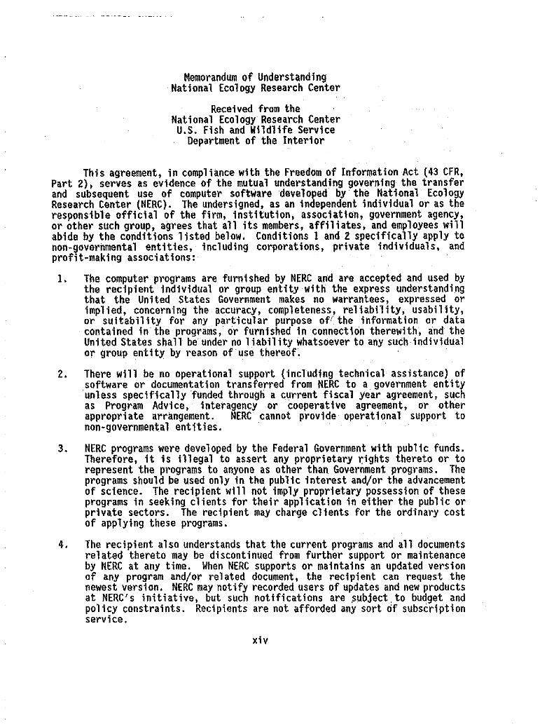
This agreement, in compliance with the Freedom of Information Act (43 CFR,Part Z), serves as evidence of the mutual understanding governing the transferand subsequent use of computer software developed by' the National EcologyResearch Center (HERC). The undersigned, as an independent individual or as theresponsible official of the firm, institution, association, government agency,or other such group, agrees that all its members, affiliates, and employees willabide by the conditions listed below. Conditions 1 and 2 specifically apply tonon-governmental entities, including corporations, private individuals, andprofit-making associations:
1. The computer programs are furnished by HERe and are accepted and used bythe recipient individual or group entity with the express understandingthat the United States Government makes no warrantees, expressed orimplied, concerning the accuracy, completeness, reliability, usability,or suitabil ity for any particular purpose of( the information or datacontained in the programs,or furnished in connection therewith, and theUnited States shall be under no liability Whatsoever to any such individualor group entity by reason of use thereof.
Z. There will be no operational support (including technical assistance) ofsoftware or documentation transferred from HERC to a government entityunless specifically 'funded through a current fiscal year agreement, suchas Program Advice, interagency or cooperative agreement, or otherappropri ate arrangement. HERe cannot provide operationa1 support tonon-governmental entities.
3. HERC programs were developed by the Federal Government with public funds.Therefore, it is illegal to assert any proprietary rights thereto or torepresent the programs to anyone as other than Government programs. Theprograms should be used only in the public interest and/or the advancementof science. The recipient will not imply proprietary possession of theseprograms in seeking clients for their application in either the public orprivate sectors. The recipient may charge clients for the ordinary costof applying these programs.
4. The recipient also understands that the current programs and all documentsrelated thereto may be discontinued from further support or maintenanceby NERC at any time. When HERC supports or maintains an updated versionof any program and/or related document, the recipient can request thenewest version. HERC may notify recorded users of updates and new productsat HERC's initiative, but such notifications are subject to budget andpolicy constraints. Recipients are not afforded any sort of SUbscriptionservice.
xiv

5. All recipient-modified program source code and documentation shouldacknowl edge the appropri ate source of the parent computer program andalgorithm. The recipient shall not represent modified HERC programs ordocumentation or outputs from the programs as original HERC products.Reference shall be made to .the HERC software, as modified by the recipient.Recipients who modify or enhance HERC software shall notify NERC of theprograms and/or algorithms modified and shall provide NERC with copies ofthose changes. NERC reserves the right to provide future revisions andenhancements of programs provided under this understanding. Recipientsare encouraged.not to assert proprietary rights to any enhancements becausework at NERC may duplicate or surpass their efforts.
6. If the source code or documentation of NERC programs is transferred toathird party, a.copy of this Memorandum of Understanding shall accompanythose products, and NERC shall be nOtified of the transfer. Thisnotification shall include the name, address, and telephone number of thethird party. Announcements of updates and releases of new NERC programsmay be provided, at NERC's initiative, to all recorded users of HERCsoftware. For purposes of this memorandum. "third party" refers to anyphysical host computer facilitY other than at the original recipient'slocation.
7. All documents and reports conveying information obtained as a result ofthe use of originalNERC programs, by either recipient or third partyusers, Shall ackn9wledge their origin as being the National EcologyResearch Center, United States D~partment of.the Interior. If the programshave been modified and/or are not longer supported or maintained by NERC,this status shall be stated in the acknowledgement.
8. The recipient understands that the acknowl edgement of the Nat ional EcologyResearch Center, U.S. Fish and Wildlife SerVice, shall notexpllcitly orimplicitly be used to support the specific analysis,interpretations, orother findings of an application or study util iZing these computerprograms. -
NERC Representative - Date
Recipient Signature - Date
xv

I. INTRODUCTION
INSTREAM FLOW INCREMENTAL METHODOLOGY
There are four major components of a stream system that determine theproductivity of the fishery (I<arrand Dudley 1978). These are: (1) flow regime,(2) physical habitat structure (channel form, substrate distribution, andriparian vegetation), (3) water quality (inclUding temperature), and (4) energyinputs from the watershed (sediments, nutrients, and organic matter). Thecomplex interaction of these components determines the primary production,secondary production, and fish population of the stream reach.
The basic components and interactions needed to simulate fish populationsasa function of management alternatives are illustrated in Figure 1.1. Theassessment process utilizes a hierarchical and modular approach combined withcomputer simulation techniques. The modular components represent the "bUildingblocks" for the simulation. The quality of the physical habitat is a functionof flow and, therefore, varies in quality and quantity over the range of the flowregime. The conceptual framework of the Incremental Methodology and gUidelinesfor its application are described in "A Guide to Stream Habitat Analysis Usingthe Instream Flow Incremental Methodology' (Bovee 1982).
Simulation of physical habitat is accomplished using the physicalstructure of the stream and streamflow. The modification of physical habitatby temperature and water qual ity is analyzed separately from physical habitatsimulation. Temperature in a stream varies with the seasons, localmeteorological conditions, stream network configuration, and the flow regime;thus, the temperature influences on habitat must be analyzed on a stream systembasis. Water quality under natural conditions is strongly influenced by climateand the geologic materials, with the result that there is considerable naturalvariation in water quality. When we add the activities of man, the possiblerange of water quality possibilities becomes rather large. Consequently, waterquality must also be. analyzed on a stream system basis. Such analysis is outsidethe scope of this manual, which concentrates on simulation of physical habitatbased on depth, velocity, and a channel index.
The results from PHABSIM can be used alone or by using a series of habitattime series programs that have been developed to generate monthly or dailyhabitat time series from the Weighted Usable Area versus streamflow tableresulting from the habitat simulation programs and streamflow time series data.Monthly and daily streamflow time series may be obtained from USGS gages nearthe study site or as the output of river system management models.
1.1

Physical
~> principal flowstructure of
l-:J stream ;.. - - - -. major influence
II~
PhysicalIt habitat
I Stream
/ //1flow
I,d,,I ...Water ... K )( I "- ~
Fish
- 1,1 J quality population.II \1N
11 (I\1.1 ~.
I\\" Temperature
\\\ ~.Primary I >1
Secondary
~\production production
t Watershed
Figure 1.1. Basic components and interaction flow for fish population simulation.
PURPOSE OF THE PHYSICAL HABITAT SIMULATION SYSTEM (PHABSIM)
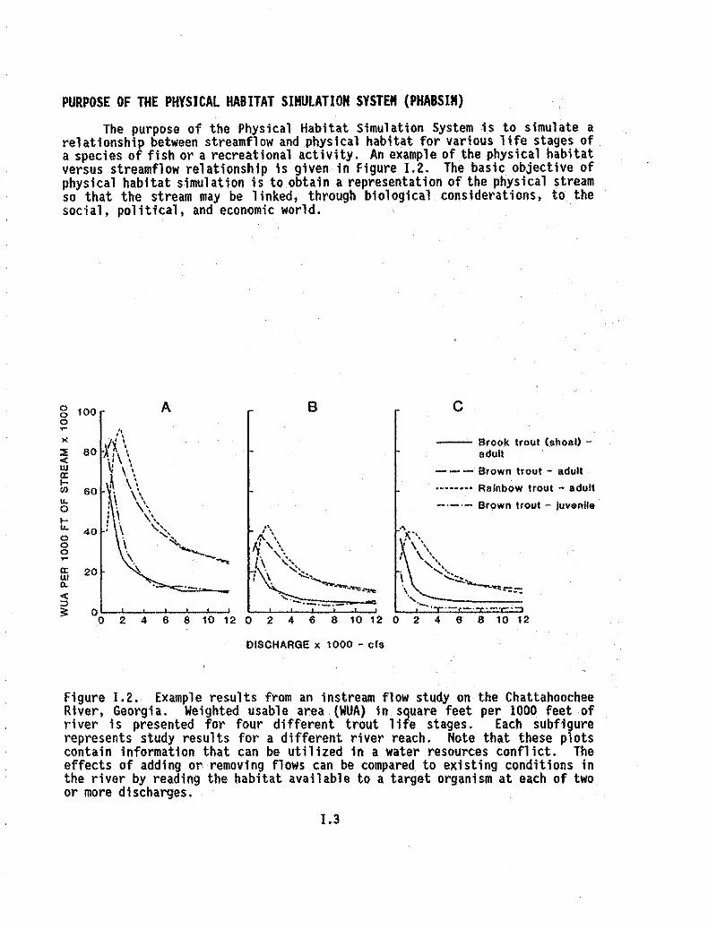
The purpose of the Physical Habitat Simulation System is to simulate arelationship between streamflow and physical habitat for various life stages ofa species of fish or a recreational activity. An example of the physical habitatversus streamflow relationship is given in Figure 1.2. The basic objective ofphysical habitat simulation is to obtain a representation of the physical streamso that the stream may be linked, through biological considerations, to thesocial, political, and economic world.
6 8 10 12
c
- Bro<>k Iroul ($hoal) -adult
- - - Brown trout - adult
.----.-. Rainbow trout - adull
_._.- Brown trout ..... juvenife
8 10 12 0 2 4
BA
'.'.)( I~ \~ 80 ~:\ \~ ~ \ \I- A \ \tI> 60 . \'u. \ \\o \ \\t: 40 \ ~~..g \ "...o . ..................... \. .......~a: 20 "-WD-o<:::l;: 0 '"--'--'--'--'--.L.--'o 2 4 6 8 10 12 0 2 4 6
g 100o~
DISCHARGE x 1000 - cIs
Figure 1.2. Example results from an instream flow study on the ChattahoocheeRiver. Georgia. Weighted usable area (WUA) in square feet per 1000 feet ofriver is presented for four different trout 1ife stages. Each sUbfigurerepresents study results for a different river reach. Note that these plotscontain information that can be utilized in a water resources conflict. Theeffects of adding or removing flows can be compared to existing conditions Inthe river by reading the habitat available to a target organism at each of twoor more discharges.
1.3

In water allocation decisions, it is desirable to know the relationship.between benefits and streamflow for the various .uses. In general, the benefitof an out~of-stream use can be quantified in terms of some type of productionfunction that relates the quantity of water used to the benefits produced.Unfortunately, little work has been done to relate the quantity of flow instreamto the benefits produced by that flow. Prior to about 1973, instream flowassessments typically arrived at a single streamflow value--a "minimum flow"above which all flows were considered available for out-of-stream use. Theseflow recommendations were determined from analyses of hydrologic records and/orfish population studies. Because of Inherent threshold concepts, theseapproaches prOVided only limited opportunity for negotiation and compromise.
, In order to improve the ability to make measurable tradeoffs between thevarious uses, a simulation system called PHABSIM has been developed to analyzeand display the relationship between streamflow and physical habitat, or betweenstreamflow and recreational river space. This relationship is a continuousfunction between the physical habitat and the streamflow. It can be used toexami ne the tradeoff between the value of water used instream with the water usedout-of-stream. Therefore, tradeoffs can be made between alternative uses andmutually acceptable management criteria developed. The decision as to the "best"allocation of the available water is a matter of negotiation among variousinterest groups.
The use of physical h.ab.ltat as a substitute for a production functionassumes the production of benefits (fish or recreation) is limited by theavailability of physical habitat. This assumption is not always true. In somesituations the production will be limited by water quality (i.e., acid rain inthe Canadian Shield region) or by the activities of man (i.e., over-harvestingof some species). In essentially all situations, physical habitat is anecessary, but not sufficient, factor for the production (If benefits. Theanalyst must never lose sight of the importance of factors other than physicalhabitat. . ,
Other papers that discuss the application of PHABSIM to water managementconcerns are "Instream Flow Values as a Factor in Water Management" (Milhous1983) and "Comparison of Minimum Instream Flow Needs" (Milhous 1986).
As an example of the application of the system, let us first look at aninstream flow study of the Chattahoochee River in Georgia. The purpose of theChattahoochee' River instream flow study was to determine the effects ofreregulation of releases from a peaking hydropower project on recreationalactivities and a put-and-take trout fishery (Nestler et al. 1986). Reregulationof the highly fluctuating flows (550 to 8000 cfs on most weekdays) from thepeaking project by a smaller reregulatlon dam would result In steady flows ofabout 1050 efs. The steady flow of 1050 cfs from the reregulation dam wouldprovide a more dependable source of water supply for the metropolitan Atlantaarea.
The study had most of the elements normally associated with instream flowstudies. That Is, the flow needs of aquatic biota, recreational activities, andmunicipal water supply were all in potential conflict. Each of theactivities/species had advocates, and a number of vocal interest groups were
1.4

involved in the controversy. PHABSIM was used to generate relationships betweeneach activity/species and discharge, as shown in Figure 1.2. This study wasbiologically simple because only adult and juvenile life stages neededassessment, since natural reproduction of trout in the tailwater has never beenobserved.
In contrast to the biological simplicity, the water resources conflict wascomplex. The habitat requirements of the three life stages peaked at differentdischarges, and the optimum flow conditions for each of the differentrecreational activities differed significantly. In other words, "everythingseemed to conflict with everything else." The results from the PHABSIM analysiswere used to generate a conflict matrix (Table 1.1) to allow decisionmakers tocrystallize the conflicts in flow requirements for each of the differentrecreat iona1 uses and trout li fe stages. The resu1 ts of the instream f1 owanalysis could then be used to optimize as many of the uses of ChattahoocheeRiver water as possible. This and other examples of the use of PHABSIM are given·in "Instream Habitat Modeling Techniques" (Nestler, Milhous, and layzerI988).
STRUCTURE OF PHABSIH
The two basic components of PHABSIM are the hydraul ic and habi tatsimulations of a stream reach utilizing defined hydraulic parameters and habitatSUitability criteria. Hydraulic simulation is used to describe the area of astream having various combinations of depth, velocity, and channel index as afunction of flow. This information is used to calculate the Weighted Usable Areaof the stream segment from suitability information based on field sampling of:the various species Of interest. The objective of thi s manual is to explainthe procedures reqUired to effectively utilize these components.
This manual presents Version II of the Physical Habitat Simulation System.The user's manual for Version I is Milhous, Wagner, and Waddle (1981). The majorprograms used by PHABSIM Version I are illustrated by Figure 1.3. The majorprograms used in Version iI are illustrated in Figure 1.4.
In Version I there were essentially two steps. The first was to dohydraulic simulation and the second was to do habitat simulation. The use ofVersion I was relatively simple and strai9htforward.
in Version Ii th~ system has four steps. The first is to simulate watersurface elevations, the second is to simulate velocities, the third is tosimulate the physical habitat versus streamflow relationship, and the fourth isto simulate the physical habitat when combinations of flows are involved.
The first step in Version I did the same as the first two steps ofVersion Ii but in essentially one step. in Version II the steps are specificand distinct. The use of Version Ii requires much more understanding of PHABSIMand the application of the results of Version I. The user must select betweenhydraul it simulation programs and alternatives, select an approach to us ing thechannel index, and select amon~ the habitat simulation models.
1.5

Table 1.1. Example conflict matrix based on optimum flow requirement for angling, river recreation,and trout life stages for the Chattahoochee River. The effect of increased flows for water supply oneach of the competing uses of river water can be seen under the rightmost column.
"""Trout Angling Rafting Canoeing
"""
Life stage! Brown trout Adult Adult Boat Novice Wateractivity Juven Adult Brook Rainbow Wading Tublng Nopwr Power Normal Prefr Midleve1 Landing Nov1ce Midlevel supply
Trout
Juveftile brown 0 0 II 0 0 II X X II XX 0 II XX +Adult. brown- 0 M 0 0 M-X X X 0·11 XX 0 II XX +Adult brook II-X 0 O-M X XX X II XX 0 II XX +Adult rainbow II M 0 X X 0 XX II 0 XX +
~,
\o{ading 0 0-11 X XX II XX 0 XX XXTubing 0-11 X XX II XX 0 XX XX
.... Boat-N"opwr X XX 0 XX II-X 0 XX +Boat-Power 0 X XX XX X XX +
'" Rafting
NovicewNormal XX XX XX XX XX +Nov;ce"Prefr XX XX 0 XX +Hidlevel XX XX 0 +landing X XX
Canoelf1g
Novice. XX +Mldlevel +
o = No conflict. optima usu.ally within 500 cfsII = Hoderate conflict. optilllll usually ..ithln SOO to 1.000 tisX =Exteos;veoonflict. optima usually within 1.000 to Z.OOO'cfsXX = Very extensive conflict, optirnamore than 2,000 cfs apart+ = Increasedflow$ for water supply beneficial- ~ Increased flows for,water supply detrimental

~~to~
...............,............
.
..q-0..
(!)C
/)LL
.3=-
-
1.7
..u,~
'"~0-'" J:....~Q-,~
....~Q';;{EM.-

HABITAT SIMULATION,
AVPERM
IFG4
Velocities :!;;;I~
i .IAVDEPTH!·~C!;;;Dlr=SCHARGEl:: ____
~ .
DISCHARGE
1HABlAl I ·11--1·.;;; f.il;:::=
IHABTAV ~. 11_ DISCHARGE
DISCHARGE
WSP
HEC2
MANSO I i
STGOS4 1-1---'
HYDRAULIC SIMULATION
Water SurfaceElevations
.<»
HABTAE I !. 11-- -DISCHARGE
HASlAM I ·11-----DISCHARGE
Figure 1.4. Major linkages for Version II of the Physical Habitat Simulation System.

OUTLINE OF THE THEORY
The basic equation used in physical habitat simulation is
WUA{Q) .. fAf(V,d,Ci) dA
where WUA(Q) is the physical habitat at the streamflow Q (also called theweighted usable area), dA is an incremental area, A is the total area at thestreamflow Q, v is the velocity, d is the depth, ci is an index to the channelcharacteristics after a combination of a substrate index and a cover index,although other forms of a channel index are possible.
The equation above can also be represented as the sum of areas within alarger reach of stream. In this case the sum is
nWUA(Q) .. X f[v(i) * d(l) * ci(i)]
i=1
in which the reach has been divided into n cells and v(i), d(i), ci(i) are theaverage values for the variable within a specific cell (cell i in this case).
Three feasible functions, f( ), are used; these are:
f(v,d,cl) .. g(v) * h(d) * k(cl)
= min g[(v) * h(d) * k(ci)]
= [g(v) * h(d) * k(cl )]1/3
where g( ) is some function of the velocity, h( ) is some function of the depth,and k( ) is some function of the stream channel index, usually substrate and/orcover. The velocity and depth vary as the streamflow changes, but it is assumedthe channel index does not. The user may also define any type of functiondesired so long as it uses combinations of velocity, depth, and a channel index.The first function (simple multiple) assumes each factor has an input on thecombined results no matter whether the other factors are high or low; the second(minimum) assumes only one factor, the one that is a minimum, has an input onthe combined results; the third (geometric mean) assumes the input on thecombined factor to be based on all three, but there are compensatory linkagesbetween the three factors. The user must select between the various forms. See"The Use of Habitat Structure Proterenda for Establishing Flow Regimes Necessaryfor Maintenance of Fish Habitat" (Stalnaker 1980) for additional information onthe nature of the habitat model.
Temperature can also be considered in the physical habitat simulation ifthe SUitability of habitat as a function of temperature is available. Thefunction for temperature is used in the equation below:
WUA' (Q) .. WUA(Q) x m(T)
1.9
where WUA'(Q) is the weighted usable area modified for temperature effect, m( )is a function of temperature, and T is the temperature. An Instream FlowInformation Paper is available that should help in addressing temperature aspectsof physical habitat modeling (Bartholow 1989).
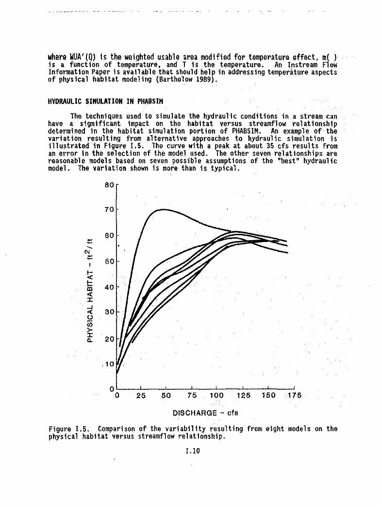
HYDRAULIC SIMULATION IN PHAI!SIM
The techniques used to simulate the hydraulic conditions in a stream canhave a significant impact on the habitat versus streamflow relationshipdetermined in the habitat simulation portion of PHABSIM. An example of thevariat ion resulting from alternative approaches to hydraul ic simul ation isillustrated in Figure 1.5. The curve with a peak at about 35 cfs results froman error in the selection of the model used. The other seven relationships arereasonable models based on seven possible assumptions of the "best" hydraulicmodel. The variation shown is more than is typical.
80
70
60...-50
40
30
20
10
25 50 75 100 125 1.50175
DISCHARGE - cfs
Figure 1.5. Comparison of the variability resulting from eight models on thephysical habitat versus streamflow relationship.
1.10

The hydraulic simulation programs in PHABSIM assume that the shape of thechannel does not change with streamflow over the range of flows being simulated.The results of the hydraulic calculations are water surface elevations andvelocities. The water surface elevations are one-dimensional in that the samevalue is used for any point on a cross section. In contrast, the velocity variesfrom point-to-point across any cross section. The hydraulic models also assumethe water surface elevations are effectively independent of the velocitydistribution in the channel.
The approaches available for the calculation of the water surfaceelevations are (1) the stage-discharge relationships, (2) the use of Manning'sequation, and (3) the standard step backwater method. The usual application ofPHABSIM requires at least one set of water surface elevations to calibrate themodel used. It is a rare application that does not have at least one set ofwater surface elevations available for calibration of the model s. In manysituations a mixture of models is used to determine the water surface elevationsin a river and for a specific flow range. This mixture may vary by cross sectionor it may vary by flow range.
Calcylation of Water Syrface Elevations
Three techniques used to simulate water surface elevations are (I) the useof an empirical stage-discharge equation based unmeasured data, (2) the use ofManning's equation, and (3) the use of·the standard step backwater method.
The standard step backwater method starts from a cross section where thewater surface elevation is known and determines the water surface elevation atthe next upstream cross section by calculating the energy .loss between the twocross sections. The energy loss is calculated using the Manning equation. Thewater surface elevation at the first Cross section must be determined in orderto start the calculations. .This starting water surface elevation may becalculated using either Manning's equation or the stage-discharge relationship,or it may be measured.
The empirical stage-discharge relationship used is
Q m a{WSl-STZ)1where Q is the discharge, WSl is the water surface elevation, STZ is the stageof zero flow, and Q and 1 are empirically derived coefficients. Rantz et al.(1982) reported that the value of 1 .is commonly between 1.3 and 1.8, and rarelyas high as 2.0, for channel control. For section control, the value of 1 almostalwaYS exceeds 2.0.
The roughness also is a function of the streamflow. An empirical equationrelating a discharge and roughness is
n .. n (JL)~o Qo
where no is the roughness at discharge Qo and n is the roughness at discharge Q.P is an empirical coefficient. The value of P is between 0 and -0.35 for gravel
1.11

QS
and cobble rivers without significant bank roughness (Milhous 1987). Forchannels with significant bank roughness, the value of Pcan be positive.
The use of Manning's equation assumes the condition of the channel controlsthe water surface elevation. In many rivers, the water surface elevation willbe controlled by rock ledges,by riffles comprised of boulders and cobbles, bygravel bars, and by constrictions In the Width of the channel.
Many rivers have compound control, with section control during low flowsand channel control for higher flows. As a result of compound control, theexpected stage-discharge relationship calculated in the IFG4 program is used forthe lower flows, and water surface e1evations determi ned using MANSQ are usedfor higher flows.
The standard step backwater calculations are used to determine the watersurface elevations at cross sections in which the water surface elevation iscontrolled by the hydrologic conditions at some downstream section. Thecalculations use Manning's equation to determine the energy loss betweensections.
In some situations, variable backwater occurs, and the WSP program is usedto simUlate water surface elevations. In relatively steep and rough streams,a mixture of stage-discharge, Manning's equation, and step backwater calculationsis needed to determine water surface elevations.
Calculation of Velocities
The velocity distribution across a channel is calculated using theempirical observations on which Manning's equation is based. The channel isdivided into cells and the velocity calculated for each of these cells •. Thephysical habitat is calculated on a cell-by-cell basis using these velocities.
The velocity in the cell k is calculated using the equation
v(k) • [a(k) r(k)O.667l/n (k)
n~ [a(j) r(j)O.0667]/n(j)j"l
where a(j) is the area of the cell j, r(j) is the hydraulic radius of the cellj, n(j) is the roughness of the cell j, and nc is the total number of wet cellsin a cross section. QS is the streamflow for which the velocity is beingcalculated.
For one set of velocity measurements, an apparent roughness is calculatedfor each measured velocity, j, using the equation
n(j) " 1.49 * ~13j)O.667l S1/2
LIZ

464
---- 870 cIs
-'-'- 495 cIs
------96 cfs
-; 460.!I
Zo 456i=«>w
. uJ 452
--------------._._._.-.-._._._.-
448 L.-.._..I-_-'-_-'-_--1._--'_~'---'
60 90 120 150 180 210 240 270
DISTANCE - feel
---- 870 cIs
-'-'- 495 .cls
------ 96 cis
1.00
2.50
0.50
3.00~I
t, I,.,\1" 1
" I I I(\' I! 1 I
: r..Ji \ PI",I t... \",,1.\/ ,\111/" '\\'1/1\, .-' ~ ,I \
1".\/ \~\J "/ u \ \I / . . II .-j '. \I / ... \I ' \ ,1/ f\, '\'I /. , '\, ....., I,.....,\....... \1', 'I' r...' \ '.._, t \,/,-..1 \' \'\ot
II • '. ~ I. \0.00 '--_..L-.L--W_-'-_........_--'-::--'-:"lL---'60 90 120 150 180 210 240 270
I
>- 1.50t:oo-'w>
o
'"~ 2.00......
DISTANCE ~ feet
Figure 1.6. Cross-sectional shape and velocity distribution in Sportsman'sPool, Salmon River, New York.
1.13

where d{j) is the depth at the vertical i, and v(j) is the velocity at verticalj. The roughness n(j} is then used to calculate the velocities for each verticalusing the water surface elevation for the discharge for which velocities arebeing simulated. The slope, S,is either selected by the user or is set to0.0025 by the program. The water surface elevation is determined using thetechniques presented previously.
An example of the velocity distribution in a typical river is given inFigure 1.6. Each velocity set would be used to simulate a range of flows, forexample, 0 to 250 cfs for the 95 cfs set. 250 to 650 cfs for the 495 cfs set,and above 650 cfs for the 870 cfs set. This means the velocities at the boundaryof the range for each set will not be the same. This will have an impact on thesimulated physical habitat, but the impact is usually not significant.Nevertheless, the difference in velocity at the boundary should be reviewedbefore doing the habitat simulation.
One concept that can be used is to determine empirically the parametersa' and P' in the following equation and use this equation to determine thevelocities in a vertical
vO} • a' elf
Each of the two techniques for simulating the velocities can be used atthe option of the user.
The Hydraulic Sjmulation Programs
The paths through the PHABSIM system that use hydraulic simulation areillustrated in Figure L7. Figures 1.8, 1.9, and 1.10 illustrate the flow ofinformation through the Curve Maintenance Programs, Habitat Simulation Programs,and the Effective Habitat Analysis Programs.
The principal hydraulic simulation programs in PHABSIM, shown inFigure 1.7, are discussed briefly below.
liSP: The Water Surface Profile Program (liSP) uses the standard stepbackwater method to determine water surface elevations. In the process,velocities are calculated which may be used in habitat simulation if velocitymeasurements needed to calibrate IFG4 are not available. The model is calibratedto predict water surface elevations by adjusting the Manning's roughness givenin the data set.
1f§!: The IFQ4 program uses a stage-discharge relationship to determinewater surface elevations unless they are supplied in the input data set. Whenusing the stage-discharge relationship, 'each cross Section is treatedindependently of all others in the data set. The velocities are determined usingtechniques based on Manning's equation.
1.14

The program is calibrated to a set of measured velocities. The usualpractice is to use at least one or more sets of velocities although the programcan be used when no velocity measurements are available.
~: This program is not part of PHABSIM, but can be used to determinewater surface elevations. The HEez program uses step backwater calculations todetermine· water surface elevations. The HECZ program was developed, and issupported by, the Hydrologic Engineering Center of the U.S. Army Corps ofEngineers, Davis, California.
~: The MANSQ program uses Manning's equation to calculate watersurface elevations. The model is calibrated using one set of water surfaceelevations. Each cross section is simulated independently of all other crosssections in the data set.
Hanning's equation isQ a 1.49 RZ/ 3 A Sl/Z
n
where Q is the discharge, n is the roughness, R is the hydraulic radius, A isthe cross section area, and S is the energy slope. In most applications of HANSQthere are two unknowns: the roughness and the energy slope. letting
K = 1.49 sl/2n
and rewriting the Manning's equation given Kwe have
Q a K R2/ 3 A
and we now have one unknown (K) which Can be determined using one ·set of watersurface elevations to calibrate the model. The. valUe of ~ can be assumed to bea constant or a power function of the discharge or the hydraulic radius.
1.15

HYDRAULIC S1MULAllON PROGRAMS GROUP
~
(1) _ walerStritt:il:Elwallon S1l11lia1on(2). Velocity SimubliIott(3} .. waIerSurraeo~lI;nd~~
wsa<TI\PE'
~
HEC2m
,~l
''''4[~''" }------l
-.....0>
• TheTAPE3li'om.o WSP !VIdoet. mt comaEnctmnnel index..codes. TheTAPE3 rtcm en F&4nm~lhiJ~~lr~fn:l:m1h!t-_....
Figure 1.7. Flow of information through PliABSIM - Hydraulic Simulation Programs Group.

CURVE MAINTENANCE PROGRAMS GROUP
..............
Suitability-of-use curve ! • Iset data
GCURV
LPTCRV(checks data inFISHCRV file)
CRVFIL
Figure 1.8. Flow of information through PHABSIM • Curve Maintenance Programs Group.

HABITAT SIMULATION PROGRAMS GROUP
HABINS
ZHAQF. habitat .... vs. flow dataZHCF. unformatted 0011 a,••• and 0011 w.ighted usable "'••• data
Figure 1.9. Flow of information through PHABS1M ~ Habitat Simulation ProgramsGroup.
I.18
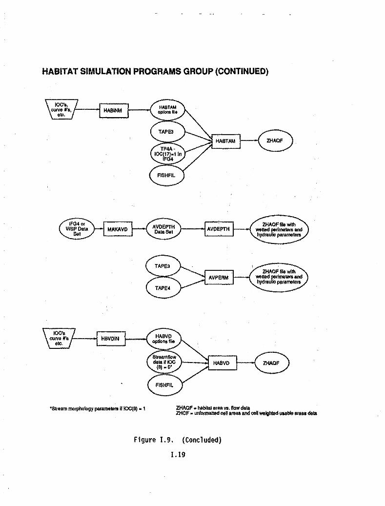
HABITAT SIMULATION PROGRAMS GROUP (CONTINUED)
t--""! AVOEPTH
1---1 HBVOIN
'Str.am morphology parame_ if 1OC(8) • I
Figure 1.9.
I--.....,;j HABVO
ZHAaF • habllal ....YO. Ilow dalaZHCF. unfoJlllllh8d cella",.. and 0011 weighted UlSbIo ..... <lola
(Concluded)
1.19
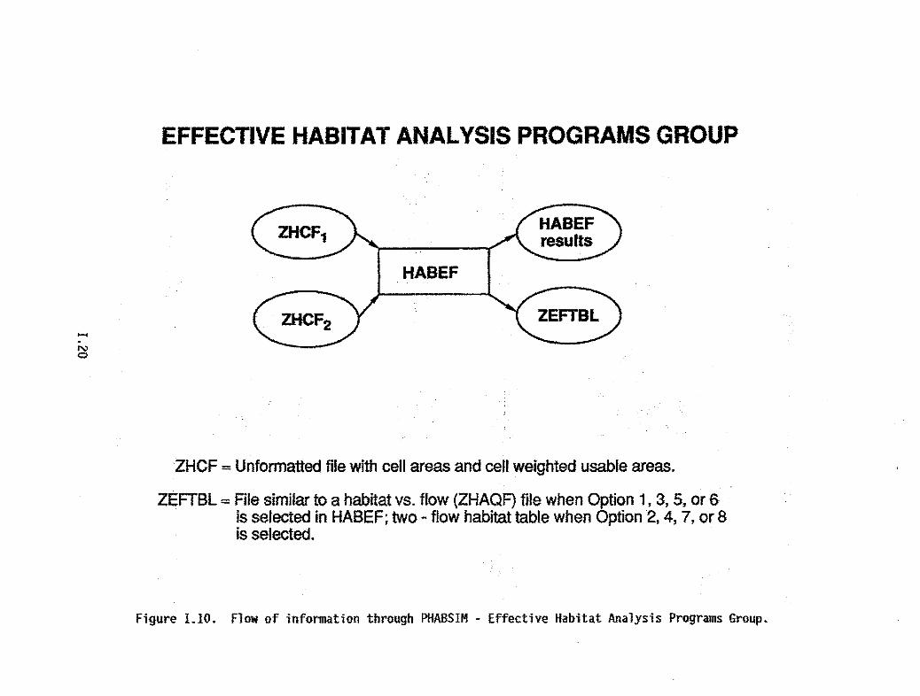
EFFECTIVE HABITAT ANALYSIS PROGRAMS GROUP
HABEF
.....N<:>
ZHCF = Unformatted file with cell areas and cell weighted usable areas.
ZEFTBL = File similar to a habitat vs. flow (ZHAQF) file when Option 1, 3, 5, or 6is selected in HABEF; two - flow habitat table when Option 2, 4, 7, or 8is selected.
Figure 1.10. Flow of information through PHABSIM - Effective Habitat Analysis Programs Group.

Hydraulic Sjmylation SUmmary
Enough emphasis cannot be placed on the importance of the three basiccategories of hydraulic input data: channel characteristics, velocities, andwater surface elevations. These are the minimum requirements for simulatingdepths and velocities as input for habitat simulation, the impetus of hydraulicsimulation.
Two important aspects associated with the practice of hydraulic simulationinclude: (1) the development of a stage-discharge relationship, or rating curve,for the cross section being considered; and (2) accurate simulation ofvel oci ties.
The stage-discharge relationship, or rating curve, is the relation betWeenthe stage, or water surface elevation, relative to an arbitrary datum, and thedischarge that existed at the time and location the water surface elevation wasmeasured. Accuracy of the stage-discharge relationships increases as moremeasurements or stage-discharge pairs are added to the curve.
In the process of obtaining discharge measurements, dividing the channelinto discrete segments and measuring the stage and velocity for each segment,velocities, channel elevations, and water surface elevations are acquired. Thedepth, calculated as the difference of the water surface elevation and channelelevation, and velocities form the base of information for predicting depth andvelocities when simulating flows.
One must be careful, however, to assure that underlying assumptions arenot unreasonably violated in order to insure predictive accuracy. A case inpoint: an assumption that the "structure of the stream channel will not bealtered by changes in flow regime" may be invalid on a stream reach particularlysubject to processes of scour and deposition. The judgement as to whethergeomorphological processes playa significant role in the behavior of the channelmust be made ..
HABITAT SIMULATION IN PHABSIM
There are two general types of habitat simulation in the Physical HabitatSimulation System: (1) a function based on the average conditions in a streamchannel and (2) a function based on the distribution of velocity and depth andthe nature of the channel ih a stream. Each of these assumes the habi tat isrelated to the nature of the stream and the conditions within the channel. Thetheory for the distribution parameter models has been presented previously. Forthe average parameter models, the theory is the same except only the wetted widthor surface is considered important.
Average Parameter Models
The average parameter models are AVDEPTH and AVPERM. Each of thesecalculates the wetted width and wetted surface for flows and water surfaceelevations supplied by the user. They also determine the width of a stream with
1.21

water over some depth specified by thll USIlI'. The avel'age velocity is alsocalculated.
Distributed Parameter Models
The programs using distribution parameters are the HABTAT, HABTAV, andHABTAE programs. The HABTAT program assumes the condition within a cellestabllshes the worth of the habitat in the cell. In contrast, the HABTAVprogram assumes the condition in a cell plus the velocity in other cells oranother location In the same cell nearby establishes the worth of the habitatin the cell.
The HABTAE program is similar to the HABTAT program with two importantexceptions. The first is that the volume (instead of the surface area) of thehabitat may be determined, and habitat conditions at each cross section can alsobe determined. In addition, the discharge does not have to be constant throughthe reach. (All the other habitat Simulation programs require cOlfstant dischargefrom cross section to cross section in the reach.)
EFFECTIVE HABITAT ANALYSIS IN PHABSIM
The effective habitat analysis (HABEF) in PHABSIH is more a determinationof the physical habitat considering. two flows, in other words, the HABitatEFfect ive when two flows are of importance. One example .of two flows is spawningflows followed by incubation flows; in this case, the spawning Is not effectiveunless the incubation maintains the habitat in condition for the eggs to hatch.A second case is the rapid change in streamflow between a "base" flow and a"generation" flow below some hydroelectric facilities.
There are two programs available for effective habitat analysis inPHABSIM. The first is the HABEf program, which compares the conditions at twoflow conditions in determining the habitat, or the conditions with two lifestages. the species cannot move from cell to cell. The second is the HABTAMprogram in which the species can move from cell to cell.
APPLICATION OF PROGRAMS
There are many paths through PHABSIM: therefore users need to keep sightof the goal, which is to develop a physical habitat versus streamflow functionbased on the nature of flow in the stream channel.
In this section certain paths are outlined as example~ to assist users indeveloping their own path through the system. These are only examples; USersmust develop their own paths based on their understanding of the problem.
The PHABSIM model can use a number of programs to determine the watersurface elevations and one model to determine the velocity distribution acrossa channel. The determination of water surface elevations and velocities isdiscussed further below.
1.22

The Use of One Ye10citY Calibration Data Set wjth IFG4
The IfG4 program can be used with only one set of velocity data tocalibrate the model. The single set of velocities is used to determine theManning's roughness (n) values which are used to distribute the flows across thecross section. These Manning's n's are effectively velocity distribution termsand not roughness in the usual energy loss Sense. The water surface elevationsmay be determined by the IFG4 program by using the stage-discharge relationshipwithin the program; or they may be determined using other, programs such as WSP,WSEI4S, MANSQ, or HEC2. If the stage-discharge relationship is used, it Isrecommended that at least three reasonable spread-out points be used (i.e., thethree points must not be for essentially the same streamflow).
The use of a single velocity calibration data set has proven to be morereliable than the use of three velocity calibration data sets in many cases-provided the water surface elevations are determined using stage-dischargerelationships based on three or more points, or by using the WSP model calibratedto water surface elevations with a stage-discharge re1atlonship'for the startingwater surface elevations. The use of the Water Surface Profile (WSP) programrequires the conditions be such that the use of WSP is appropriate. When usingthe stage-discharge relationship, the same approach is used as with the stageapproach within IFG4. The use of Manning's equation requires one set of watersurface elevations, and the assumption is made that Manning's equation is validat each cross section and there is no backwater effect at any cross section.
The use of each approach is outlined below.
When using the WSP program with a single velocity set for calibrating IFG4.the steps to follow are:
1. Collect one set of velocity me.asurements.
2. Collect water surface elevations at each cross section for at leastone streamflow.
3. Prepare and check an IFG4 data set with the single velocity data set.
4. Place the single water surface elevation for the calibration velocityset on the WSL line for each cross section and the correspondingstreamflow on a single QARD line and run the IFG4 program. Reviewthe results and select options for the production runs.
5. Convert the IFG4 data set to a WSP data set using the RI4TWSPbatch/procedure file; retain the original IFG4 data set.
6. Calibrate the WSP model to water surface elevations with constantroughness for all cells and cross sections.
7. Cal ibrate the WSP model to essential constant roughness in each crosssection, but varying from cross section to cross section if thereis a physical reason to do so. The roughness within a section canbe varied also if there is a physical reason to do so.
1.23

9. Select the streamflows needed to develop the physical habitat versusstreamflow relationship.
9. Select roughness multipliers. if appropriate.
10. Run the calibrated WSP model with the streamflows from Step 8.
11. Use the WSEI4 program to read the TAPE4 from SteP 10 and place thecalculated water surface elevations on the appropriate WSl lines inthe IFG4 data set. The streamflows from Step 8 are also.written asthe streamflows on the QARD lines in the IFG4 data set.
12. Make the production runs with the IFG4 data set.
When using the stage-discharge relationship with a single velocity set forcalibrating IFG4. the steps to follow are:
1. Collect one set of velocity measurements.
2. Collect water surface elevations at each cross section for three ormore streamflows.
3. Prepare and check an IFG4 data set with the single velocity data set.
4. Place the single water surface elevation for the calibration velocityset on the WSl line for each cross section and the correspondingstreamflow on a single QARD line and rUn the IFG4 program. Reviewthe results and select options for the production· runs.
5. Select the streamflows needed to develop the physical habitat versusstreamflow relationship.
6. Use the stage-discharge data with the WSEI4S program to create theWSl lines in the IFG4 data set for the production run.
7. Make the production run.
I.24

When using Manning's equation (MAHSQ) to determine water surface elevationsfor a single velocity set used to calibrate the IFG4 program, the steps to followare:
1. Collect one set of velocity measurements and one set of water surfaceelevations for the cross sections.
2. Prepare and check an IFG4 data set with the single velocity data set.
3. Place the single water surface elevation for the calibration velocityset on the IISl line for each cross sectiOn and the correspondingstreamflow on a single QARO line and run the IFG4 program. Reviewthe results and select options for the production runs.
4. Select the streamflows needed to develop the physical habitat versusstreamflow relationship.
5. Convert the IFG4 data set to a MANSQ data set using the 14THSQprogram; retain the IFG4 data set.
6. Use the single set of water surface elevation-discharge data withthe MANSQ program to create a TAPE4 with the water surface elevationand average channel velocities for the flows of interest.
7. Use the IISEI4 program to add the IISL lines to an IFG4 data set.
8. Make the production run.
The Use of Two or More Velocity Calibration Data Sets With IFG4
The use of two or more velocity sets to calibrate the IFG4 model tovelocities folloWS the same steps as presented in the previous section with someexceptions.
The exceptions are the range of the various sets used. If the dischargesare arrayed in increasing order and there are n sets, the ranges for each setare for Q < Qc(l) , use the lowest set of velocities to calibrate the IFG4program. For Q> Qc(n), use the highest set of velocities to calibrate the IFG4program. The range between Q(1) and Q(n) can be handled using two possibleapproaches. One is to break t~e internal into pieces and use each calibrationvelocity set for a specific range. The other approach is to use the data tocalibrate the equation
for the range Qc(l) < Q< Q(n).
For the three velocity set case, the steps are presented below as "tasks"in a manner that illustrates a different way of phrasing the work.
1.25

Ta~k 1: Collect, check, and enter the data fQr a study reach int~ inputfiles.
Task 2: Hodel the water surface elevations.
Task 3: Model the velocities.
Task 4: Select the streamflows needed for the production runs.
Task 5: Build the IFG4 production data set based on the results from Tasks2 through 4 above.
Task 6: Develop alternative channel index files as needed for the study.
Task 7: Develop a habitat input file.
Task 8: Calculate. the habitat versus streamflow relationship for eachvelocity data set. .
Task 9: Develop the "best" habitat versus streamflow functions.
SUMMARY
In this chapter, a very brief outline of PHABsni is presented. One of themajor tasks of a user is the determination of the programs most appropriate toa given problem. .
The first two tasks are the simulation of water surface elevations andvelocities using the hydraulic simulation programs. This is followed by thesimulation of habitat using one or more of the habitat simulation programs. Thefourth task, if appropriate, is the simulation of the effective habitat.
1.26

II. HYDRAULIC SIMULATION PROGRAMS
INTRODUCTION
The hydraulic simulation programs in PHABSIM assume that the shape of thechannel does notchan(le with streamflow over the range of flows being simulated.The results Qf the hydraul ic calculations are water surface elevations andvelocities. The water surface elevations are one-dimensional in that the samevalue is used for any point on a cross section. In contrast, the velocity variesfrom point-to-pointacross any cross section. The hydraulic models also assumethe water surface elevation is effectively independent of the velocitydistribution in the channel. .
The approaches available for the calculation of the water surface elevationare (I) the stage-dischar(le relationship, (2) the use of Manning's equation, and(3) the standard step backwater method. The usual appl ication of PHABSIMrequires at least one set of water surface elevations to calibrate the modelused. It is a rare application that does not have at least one set of watersurface elevations available for calibration of the models. In many situationsa mixture of models is used to determine the water surface elevations.
The velocity distribution is determined usin(l techniques based on Manning'sequation. Usually one set of measured velocities is available for calibrationof the.. mode1s.
Refer to the following figures for information on the hydraulic simulationprograms:
Figure 1.7 - "Flow of Information Through PHABSIM - Hydraul icSimulation Programs Group";
Figure Il.l - "Creating and Checking an IFG4 Data Set";Figure 11.2 - "Creating and Checking a WSP Data Set"; andFigure Il.3 - "Creating a MANSQ Data Set".
PROGRAM BATCH/PROCEDURENAME FILENAME FUNCTION PROGRAM DESCRIPTION
HEC2 HydraulicSimulation/Water SurfaceElevationSimulation
11.1
This program is not part of PHABSIM,but can be used to determine watersurface el evations. The HEC2 programuses step backwater calculations todetermine water surface elevations.The HEC2 program was developed, andis supported by the HydrologicEngineering Center of the U.S. ArmyCorps of Engineers. Refer to "HEC-2Water Surface Profil e Users Manual"for documentation.
\

HYDRAULIC SIMULATION {Continyed}
PROGRAM BATCH/PROCEDURENAME FILENAME FUNCTION
IFG4 • RIFG4PHABAR2
HydraulicSimulation/VelocitySimulation
ILl
pROGRAM DESCRIPTION
Uses .a stage-discharge relationshipto determi ne water surface eIevationsunless they are supplied in the dataset. When using the stage-dischargerelationship, each cross section istreated independently of all othersin the data set. The velocities aredetermined using techniques based onManning's. equation.
RIFG4.ZIF64.ZOOT.TAPE3.TAPE4,TP4.ZVAFF.ZVCEF
ZIFG4-IFG4 data set (input)Zour-IFG4 results (output)TAPE3-unformatted cross section andreach data (output)
TAPE4..unformaUed flow data (output)TP4-rearranged TAPE4 file. Used asinput to HA8TAT (output)
ZVAFF-velocity adjustinent factor fileCreated if 10C( 13)=1 (output)
ZVCEF-velocity calibration errors fileCreated if IOC(10)-1 (output)
NOTE: If IOC(17)"I, the TAPE4 and TP4files will be in HABTAM and HABTAVreadable format. These files needto be renamed to TAPE4A and TP4A bythe user.

HYDRAULIC SIMULAIION (Continued)
PROGRAM BATCH/PROCEOURENAME FILENAME FUNCTION
MANSQ RMANSQ HydraulicSimulation/Water SurfaceElevationSimulation
PROGRAM DESCRIPTION
Calculates water surface elevationsusing Manning's equation. The modelis calibrated using one set of watersurface elevations. Each cross sectionis simulated independently of allother cross sections in the data set.
STQqS4 RSTGQS4 HydraulicSimulation/Water SurfaceElevationSimulation
II.3
RMANSQ.ZMANSQ.lOUT.TAPE3.TAPE4
ZMANSQ-MANSQ data set (input)lOUT-MANSQ results (output)TAPE3-unformatted cross section and
reach data (output)TAPE4-unformatted flow data (output)
Determines the water surface elevationsfor an IFG4 data set using the stagedischarge relationship based on flowson the CAL lines.
RSTGQS4.ZIFG4,ZOUT.TAPE3.TAPE4
ZIFG4-IFG4 data set (input)lour-STGQS4 results (output)TAPE3-unformatted cross section andreach data (output)
TAPE4 - unfOrmatted flow data (output)

HYQRAULIC SIH~IOft (Continued}
PROGRAM BATCH/PROCEDURENAME FILENAME FUNCTION
liSP, RWSPLSTWSL &.PHABAR2
HydraulicSimulationlWater SurfaceEl evat ionSimulation
11.4
PROGRAM DESCRIPTION
Uses the standard step backwatermethod to determine water surfaceelevations. In the process, velocitiesare calculated which may be used inhabitat simulation if velocitymeasurements needed to calibrate IfG4are not available. The model iscalibrated to predict water surfaceelevations by adjust lng the Manning'sroughness given in the data set. Userhas option of listing the simulatedwater surface elevations to the screenor to an output file to be used incalibration.
RWSP,ZWSP,ZOUT,TAPE3,TAPE4,TP4,ZVOUT
ZWSP~WSPdataset (input)ZOUT~W~P results (output)TAPE3~unformatted cross section andreach data (output)
TAPE4~unformatted flow data (output)TP4*rearrranged TAPE4 fil e. Used asinput to HABrAT (output)
ZVOUT~optional output file formattedfor easy review of velocities.Created when Option 5 is on. (output)

CREATING AN IFG4 DATASET
Method 1:
1FG4IN(micro only)
Method 2:
MODQARD(addsQARD
values'
MODIOC(adds IOCvalues'
14TEXTFree· formatted fileof IFG4 input data
created with aneditor
..........'" CKI4TXT
(checks data)
CHECKING AN fFG4DATA SET
CKl4
REVl4
lREVl4 balch/procedure meruns: CKl4
REVl4LPTTHWESLOP34
IFG4Data Set
Figure 11.1. Creating and checking an IFG4 data set.
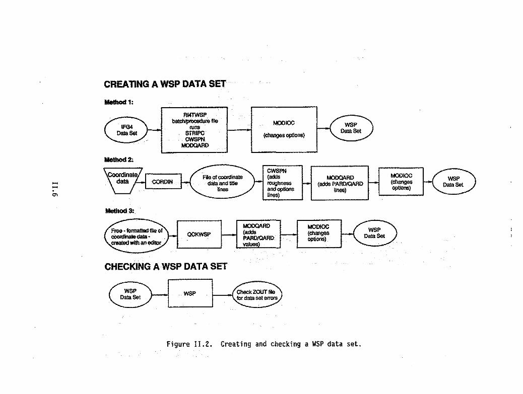
CREATING A WSP DATA SET
Method 1:
RI4TWSPbalcl1/plt)cljdUle filE>
lUllSSfRIPCCWSPN
MOOQARD
MODlOC
(c:l1anges options)
........'"
Me1llod2:
Metbad3:
CWSPN(sddsroughnessandoplionslines)
MODOARO(adds PAROIClARD
lines)
MODlOC(c:l1angesoptions)
OCKWSPMOOQAAD(addsPAADIQI\ROvalues:
MODlOC(c:l1angesoptions)
CHECKING A WSP DATA SET
W$P
Figure 11.2. Creating and checking a WSP data set.
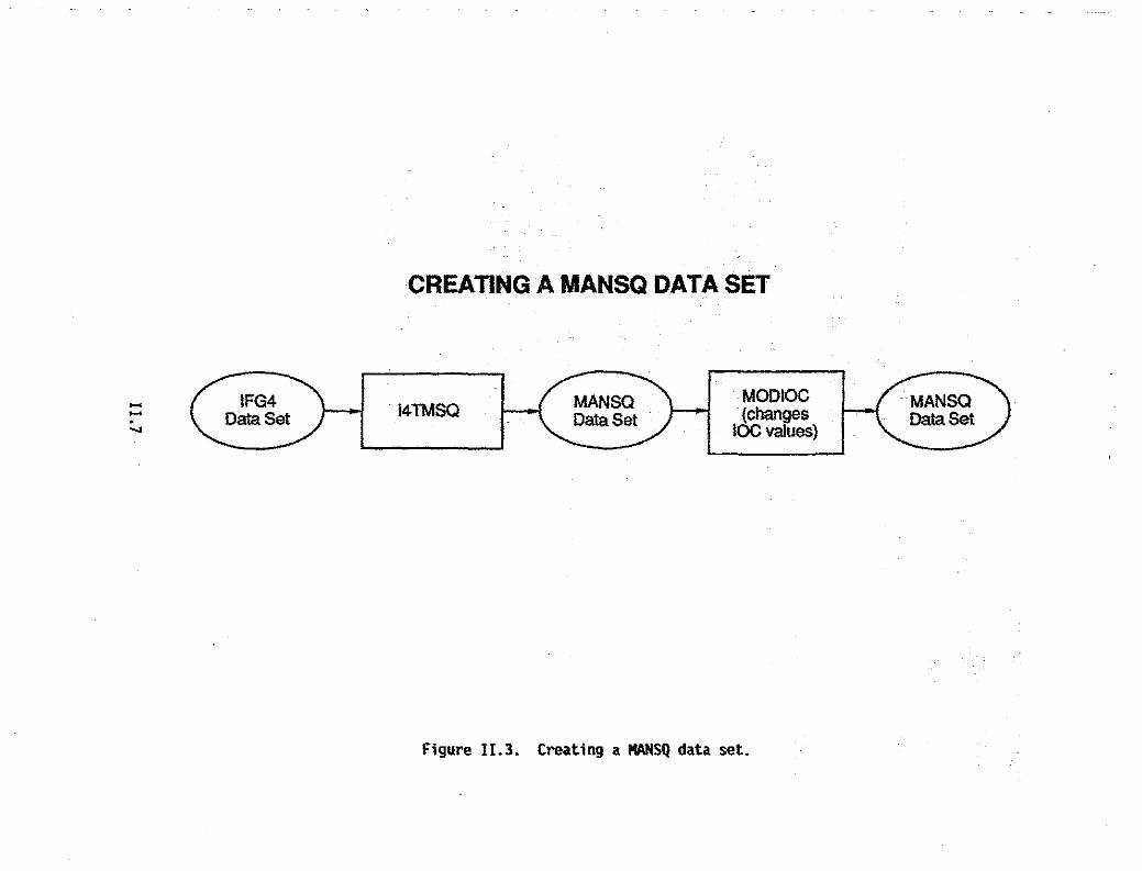
CREATING A MANSQ DATA SET
..........
.....IFG4
DataSet 14TMSQ MANSODataSet
MODIOC(changes
IOCvalues)
Figure 1I.3. Creating a KANSQ data set.

PROGRAM DESCRIPTION
IfG4 DATA SET CREATION - Appendix Acontains a sample IFG4 data set.
PROGRAM BATCH/PROCEDURENAME FILENAME FUNCTION
Creation Method 1:
IFG4IN RIFG4IN IFG4 Data SetCreation
Builds and/or edits an IFG4 data set.Micro only.
RIFG4IHUser is prompted for filename.
Creation Method 2:
CKI4TXT
I4TEXT
RCKI4TX
RI4TEXT
IFG4 Data SetCreation
IFG4 Data SetCreation
II .8
Reads the free-formatted input fileto 14TEXT and writes a detailed listingof the contents in a format that iseasy for checking. Type INFOI4T forinformat ion on the format of the freeformatted input file.
RCKI4TX,ZIN,ZOUT
ZIN=free·formatted file (input)ZOUT"'CKI4TXT results (output)
Creates an incomplete IFG4 data set(missing IOC and QARO values) with upto nine velocity sets, from a freeformatted fil e created wi th an edi tor.Type INFOI4T for information on theformat of the free-formatted inputfile.
RI4TEXT,ZIN,ZIFG4
ZIN=free-formatted file (input)ZIFG4=IFG4 data set (output)

IfQ4 DATA SET CREATION (Creation Method 2 continued)
PROGRAM BATCH/PROCEDURENAME FILENAME FUNCTION PROGRAM DESCRIPTION
IFG4 Data SetCreation
AOOCY
MODIOC
RADDCY
RMODIOC
Adds CAL and VEL lines to an existingIFG4 data set. An IOC and/or a QARDline with no values is also added ifthey do not exist in the data set.Type IHFOACV for information on theformat of the free-formatted inputfile.
RADDCV,ZIN,ZIFG4,ZIFG4N
lIN-free-formatted CAL/VEL data file(input)
ZIFG4-IFG4 data set in which to addCAL and VEL lines (input)
ZIFG4N"new IFG4 data set with CAL andVEL lines added (output)
IFG4/WSP/MANSQ/ Changes options in the selected dataHABTAT/HABTAH/ set or options file.HABTAV/HABTAE/HABVD Data Set RMODIOC,lIN,lOUTModification
MODQARD RMODQRD IFG4/MANSQ/WSPData SetModificat ion
11.9
lIN"original data set (input)ZOUT=new data set with modifiedoptions (output)
Replaces (or adds if none eXist)PARD/QARD lines in an IFG4, MANSQ, orWSP data set
RMODQRD,ZIN,lMOD,TAPE4,ZOUT
lIN=IFG4, MANSQ, or WSP data set(input)
ZMOD=IIlodified IFG4, MANSQ, or WSP dataset (output)
TAPE4=unformatted flowdata, (optionalinput). When modifying a WSP dataset, user has the option to read datafor PARD and QARD 1ines from a TAPE4or enter it manually.
ZOUT-MODQARD results (output). Thisfile is only generated if Option 1(Stage-Discharge Relationship) ischosen to generate the hydraulicdata.
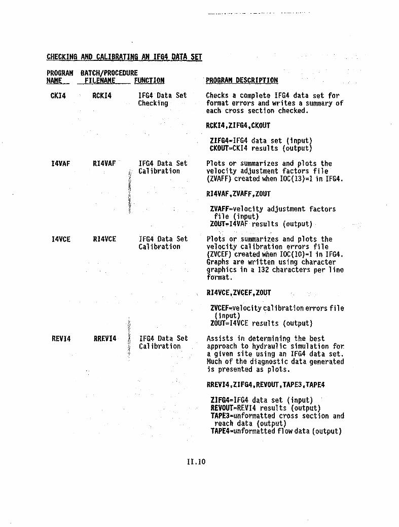
CHECKING AND CALIBRATING AN IFG4 DATA nIPROGRAM BATCH/PROCEDURENAME FILENAME FUNCTION
-_ .._--_ .. _ - - - .-. -_. - ".
PROGRAM DESCRIPTION
CKI4 RCKI4 IFG4 Data SetChecking
Checks a complete IFG4 data set forformat errors and writes a summary ofeach cross section checked.
J4VAF
I4VCE
REVI4
RI4VAF IFG4 Data Seti Calibration
."'f)~YI
RJ4VCE IFG4 Data SetCalibration
11':<
RREVI4 Z IFG4 Data Set:! Calibrationh
RCKI4.ZIFG4,CKOUT
ZIFG4-IFG4 data set (input)CKOUT=CKI4 results (output)
Plots or summarizes and plots thevelocity adjustment factors file(ZVAFF) created when We( 13}=l in IFG4.
RI4VAF,ZVAFF,ZOUT
ZVAFF=velocity adjustment factorsfile (input)
ZOUT=I4VAF results {output}
Plots or summarizes and plots thevelocity calibration errors file(ZVCEF) created.when IOC(IO}=l in IFG4.Graphs are written using charactergraphics in a 132 characters per lineformat.
RI4VCE,ZVCEF,ZOUT
ZVCEF=velocity cal ibration errors file(input)
ZOUT=[4VCE results (output)
Assists in determining the bestapproach to hydraulic simulation for.a given site using an IFG4 data set.Much of the diagnostic data generatedis presented as plots.
RREVI4,ZIFG4.REVOUT,TAPE3,TAPE4
ZJFG4=IFG4 data set {input}REVOUT=REVr4 results (output)TAPE3=unformatted cross section andreach data {output}
TAPE4=unformatted flow data (output)
II.IO

PROGRAM DESCRIPTION
CHECKING AND CALIBRATING AN IFG4 DATA SET (COntinued)
PROGRAM BATCH/PROCEDURENAME FILENAME FUNCTION
CKI4, TREVI4REVI4,LPTTHWE,&SLOP34
IFG4 Data SetCali bratton
II. 11
Generates files for a total review ofan IFG4 data set. TAPE3 and TAPE4files are generated by REVI4 and thenare used as input to lPTTHWE andSlOP34.
TREVI4.ZIFG4,CKOUT,REVOUT,LPTOUT,SLPOUT.TAPE3,TAPE4
IIFG4-IFG4 data set (input)CKOUT-CKI4 results (output)REVOUT-REVI4 results (output)lPTOUT-lPTTHWE results (output)SLPOUT-SlOP34 results (output)TAPE3-unformatted cross section andreach data (output, input)
TAPE4-unformatted flow data(output. input)

11.12

IFG4 DATA SET MODIFICATION (Continued)
PROGRAM BATCH/PROCEDURENAME FILENAME FUNCTION
MODIOC RMODIOC IFG4/WSP/MANSQ!HABTAT/HABTAM/HABTAV/HABTAE/HABVD Data SetModification
MODN
MODQARD
RMODN
RHODQRD
IFG4/WSPData SetModification
IFG4/MANSQ/WSPDataSetModification
PROGRAM DESCRIPTION
Changes options in the selected dataset or options file.
RMODIOC.ZIN.ZOUT
lIN-original data set (Input)ZOUT-new data set with moaifiedoptions (output)
Adds or modifies Nvalues for eachcross section in an IFG4 or WSP dataset.
RMODN,ZIN,ZOUT
IIN-IFG4 or WSP data set (Input)ZOUT-modified IFG4 or WSP data set
(output)
Replaces (or adds if none exist)PARD/QARD lines in an IFG4, MANSQ, orWSP data set.
RMODQRD,ZIN,ZMOD,TAPE4.ZOUT
IIH-IFG4, MANSQ. or WSP data set(input)
ZHOO-modified IFG4, MANSQ, or WSP dataset (output)
TAPE4-unformatted flow data, (opt lona1input). When modifying a WSP dataset. user has the opt ion to read datafor PARD and QARD 1Ines from a TAPE4or enter it manually.
IOUT-MODQARD results (output). Thisfile is only generated If Option I(Stage-Discharge Relationship) ischosen to generate the hydraulicdata. .
11.13

ill!.DA!A SEU!.O.!llf.IkATIPB {Con~jnued}
PROGRAM BATCH/PROCEDURENAME FILENAME FUNCTION
MODSLP
WSEI4
WSEI4D
RMODSLP
RWSEI4
RWSEI4D
IFG4/WSPData SetModification
.. I'
IFG4 Data SetHod ifi cat ion
IFG4 Data SetModificatioll
IJ.l4
PROGRAM DESCRIPTION
Modifies the slope at each crosssection in an IFG4 data set QB modi fiesthe water surface· elevation or slopefor each flow on the QARO lines In aWSP data set.
RHODSLP,ZIN,ZOUT
ZIN-IFG4 or WSP data set (input)lOUT-new IFG4 or WSP data set withmodified slopes (output)
Reads water surface elevations anddi scharges from a TAPE4 or TP4 and addsor replaces the QARD and WSL lines inan IFG4 data set.
,".
RWSEI4,ZIFG4.lIFG4N,TAPE4
ZIFG4-IFG4 data set (input)ZIFG4N-new IFG4 data set with added/replaced water surface elevationsand discharges (output)
TAPE4-unformatted flow data (input)
Adds or replaces the QARD and WSL 1inesin an IFG4 data set. Data is enteredfrom the keyboard.
RWSEI4D,ZIFG4,lIFG4N
lIFG4-IFG4 data set (input)llFG4N-new IFG4 data set with added/replaced water surface elevationsand discharges (output)

IFG4 DAtA SEI MODIFICATION {Continued}
PROGRAM BATCH/PROCEDURElIME FILENAME FUNCTION
NSEI4H
NSEI4S
RNSEI4H
RNSEI4S
IFG4 Data SetModi fication
IFG4 Data SetModi fication
PROGRAM DESCRIPTION
Reads water' surface elevati~ns anddi scharges ,from a HEC2 output f 11 e andadds or replaces the QARD and WSl 1inesin an IFG4 data set.
RWSEI4H,ZHECOUT,ZIFG4,ZIFG4N
ZHECOUT..HEC2 1ine printer output file(input)
ZIFG4..IFG4 data set (input)ZIFG4N-new IFG4 data set with added/replaced ,water surface elevationsand discharges from ZHECOUT (output)
Uses a stage-discharge relationshipto calculate water surface elevationswhich are then added to an IFG4 dataset. The user enters the stage-Q dataneeded to determine the stage-dischargerelationship.
RNSEI4S,ZIFG4,ZIFG4N,ZOUT
ZIFG4.. IFG4 data set (input)ZIFG4N=new IFG4 data set with WSl '
11nes added (output)'ZOUT=WSEI4Sresults. stage-dischargerelationships and plots (output)
ILlS

~ DATA SET CREATION . Appendix Acontains a sample WSP data set.Creation Method 1:
STRIPC, RI4TWSPCWSPN, lMODQARO
WSP Data SetCre.ation
Converts an IFG4 data set to a completeWSP data set. Each vertical becomesthe right boundary of a cell exceptthe left most vertical.
MODIOC RMODIOC IFG4/WSP/MANSQ/HABTAT/HABTAM/HABTAV/HABTAE/HABVD Data SetModification
RI4TWSP,ZIFG4.lWSP,TAPE4,ZOUT
ZIFG4=lFG4 data set (input)ZWSP=WSP data set (output)TAPE4=uriformatted flow data, (optionalinput). If not supplied, data forthe PARD and QARD lines are enteredfrom the keyboard.
ZOUT=MOOQARO results (Option 1chosento generate hydrau1 ic data) (output)
Changes options in the selected dataset or options file.
RMODIOC,ZIN,ZOUT
ZIN=origina1 data set (input)ZOUT=new data set with modifiedoptions (output)
Creation Method 2:
CORDIN RCOROIN WSP Data SetCreation
11.16
Creates, or adds to, a file ofcoordinate data and title lines. AnENOJ and an ENOR 1ine are also created.
RCOROIN,ZCORD,ZCORDIN
ZCORD=coordinate data fil e with ti t1elines (output)
ZCORDIN=coordinate data file to beadded ,to (optional input)
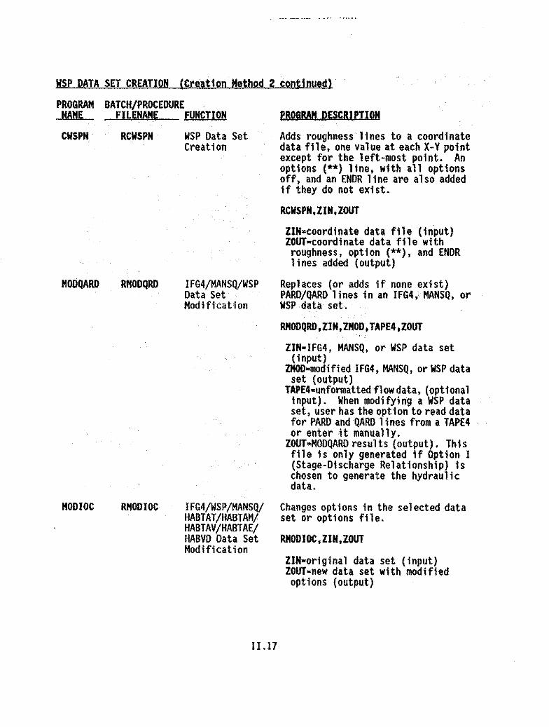
NSP DATA SET CREATION (Creation Method 2 continued)
PROGRAM BATCH/PROCEDURENAME FILENAME FUNCTION PROGRAM DESCRIPTION
CNSPN RCWSPN WSP Data Set Adds roughness lines to a coordinateCreation data file. one value at each X-V point
except for the left-most point. Anoptions (**) line. with all optionsoff. and an [NOR line are also addedif they do not exist.
RCWSPN,ZIN.ZOUT
IIN=coordinate data file (input)lOur-coordinate data file withroughness. option (**). and ENDRlines added (output)
MODQARD RMODQRD IFG4/MANSQ/WSP Replaces (or adds if none exist)Data Set PARD/QARD 1ines in an IFG4, MANSQ. orModification WSP data set.
RMODQRD,IIN.IMOD.TAPE4.10UT
ZIN-IFG4. MANSQ. or WSP data set(input)
ZMQD-modi fi ed IFG4. MANSQ. or WSP dataset (output)
TAPE4-unfonnattedflow data. (optionalinput). When modifying a WSP dataset. user has the option to read datafor PARD and QARD lines from a TAPE4or enter it manually.
ZOUT=MODQARD results (output). Thisfile is only generated if Option I(Stage-Discharge Relationship) ischosen to generate the hydraulicdata.
MODIOC RMODIOC IFG4/WSP/MANSQ/ Changes options in the selected dataHABTAT/HABTAM/ set or options file.HABTAV/HABTAE/HABVD Data Set RHODIOC. lIN. lOUTModificat ion
liN-original data set (input)lOUT-new data set with modifiedoptions (output)
11.17

WSP DATA SET CREATION (Continued)
PROGRAM BATCH/PROCEDURENAME FILENAME FUNCTION PROGRAM DESCRIPTION
Creation Method 3:
QCKWSP RQCKWSP WSP Data Set Creates an incomplete WSP data setCreation (missing PARD and QARD values) from
a free-formatted file created with aneditor. Type INFOQWP for informationon the format of the free-formattedinput file.
RqcKMSP,ZIN,ZWSP
ZIN=free·formatted coordinate datafile (input)
ZWSP=WSP data set (output)
MODQARD RlIODQRD IFG4jMANSQ/WSP Replaces (or adds if none exist)Data Set PARD/QARD 1ines in an IFG4, MANSQ, orModification WSP data set.
RMODQRD,ZIN,ZMOD,TAPE4,ZOUT
ZIN=IFG4, MANSQ, or WSP data set(input)
ZMOD=modified IFG4, MANSQ, or WSP dataset (output)
TAPE4"unformatted flow data, (optionalinput). When modifying a WSPdataset, user has the option to read datafor PARD and QARD lines from a TAPE4or enter it manually.
ZOUT"MQDQARD results (output). Thisfile is only generated if Option 1(Stage-Discharge Relationship) ischosen to generate the hydraulicdata.
MODIOC MODIOC IFG4/WSP/MANSQ/ Changes options in the selected dataHABTAT/HABTAH/ set or options file.HABTAV/HABTAE/HABVD Data Set RMODIOC,ZIN,ZOUTModification
ZIN"original data set (input)ZOUT=new data set with modifiedoptions (output)
ILlS

CHECKING A\liSP DATA SET
PROGRAM BATCH/PROCEDUREHAME FILENAME FUNCTION
\liSP, R\IISPLSTWSL, 1PHABAR2
HydraulicSimulation
PROGRAM DESCRIPIION
Data set errors wi 11 be 11 sted In theZOUT file.
RWSP,ZWSP,ZOUT,TAPE3,TAPE4,TP4.ZVOUT
ZWSP-NSP data set (input)ZOUT-WSP results (output)TAPE3-unformatted cross section andreach data (output)
TAPE4..unformaUed flow data (output)TP4-rearranged TAPE4 file. Used asinput to HABTAT (output).
ZVOUT-optional output file formattedfor easy review of velocities.Created when Option 5 is on. (output)
NSP DATA SET MODIFICATION
NODIOC RMODIOC IFG4/WSP/MANSQ! Changes options in the selected dataHABTAT/HABTAM/ set or options file.HABTAV/HABTAE/HABVD Data Set RMODIOC,ZIN,ZOUTModification
MOON RMODN IFG4/WSPData SetModification
lUg
ZIN-orlginal data set (input)ZOUT-new data set with modifiedoptions (output)
Adds or modifies Nvalues for eachcross section in an IFG4 or NSP dataset.
RMODN,ZIN,ZOUT
ZIN-IFG4 or NSP data set (input)lOUT-modified IFG4 or NSP data set(output)
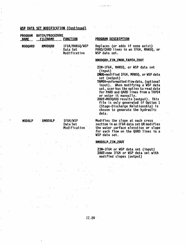
NSP DATA SET MODIFICATION (Continued)PROGRAM BATCH/PROCEDUR~
NAME FILENAME FUNCTION
MODQARD RMODQRD IFG4/MANSQ/WSP. Data Set
Modification
MODSLP . RMODSLP . IFG4/WSPData SetModificat ion·
11.20
PROGRAM DESCRIPTION
Replaces (or adds if none exist)PARD/QARD lines in an IFG4, MANSQ, orWSP data set.
RMODQRD,ZIN,ZMOD,TAPE4,ZOUT
ZI~=IFG4, MANSQ, or WSP data set(input)
ZMOO..modified IFG4. MANSQ, or WSP dataset (output)
TAPE4..unfonnatted flow data, (optionalinput). When modifying a WSP dataset, user has the option to read datafor PARD and QARD 1ines from a TAPE4or enter it manually.
ZOUT..MODQARD results (output). Thisfile is only generated if Option I(Stage-Discharge Relationship) ischosen to generate the hydraulicdata.
Modifies the slope at each crosssectlonin an IFG4 data set OR modifiesthe water surface elevation or slopefor each flow on the QARD lines in aWSP data set.
RMODSLP,ZIN,ZOUT
ZIN=IfG4 or WSP data set (input)Zour-new IFG4 or WSP data set withmodified slopes (output)
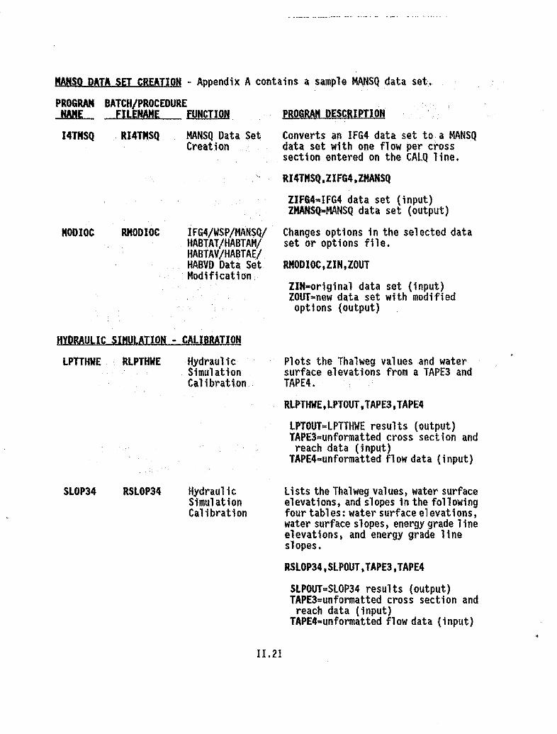
PROGRAM DESCRIPTION
MANSO QATA SET CREATION - Appendix Acontains a sample MANSQ data set.
PROGRAM BATCH/PROCEDURENAME FILENAME FUNCTION
MANSQ Data SetCreation
I4THSQ
MODIOC
RI4T11SQ
RMODIOC
Converts an IFG4data set to a MANSQdata set with one flow per crosssection entered on the CAlQ line.
RI4TMSQ,ZIFG4.ZMANSQ
ZIFG4-IfG4 data set (input)ZMANSQ-MANSQ data set (output)
IFG4/WSP/MANSQI Changes options in the selected dataHABTAT/HABTAM! set or options file.HABTAV/HABTAE/HABVO Data Set RMODIOC,ZIN,ZOUTModification
ZIN-original data set (input)ZOUT-new data set with modifiedoptions (output)
HYDRAULIC SIMULATION - CALIBRATION
LPnHllE RLPTHlIE HydraulicSimulationCalibration
Plots the Thalweg values and watersurface elevations from a TAPE3 andTAPE4.
RLPTHWE.LPTOUT.TAPE3.TAPE4
LPTOUT=lPTTHWE results (output)TAPE3=unformatted cross section andreach data (input)
TAPE4-unformatted flow data (input)
SLOP34 RSLOP34 HydraulicSimulationCalibration
11.21
Lists the Thalweg values, water surfaceelevations, and slopes in the followingfour tables: water surface elevations,water surface slopes, energy grade lineelevations, and energy grade lineslopes.
RSLOP34,SLPOUT.TAPE3,TAPE4
SLPOUT=SLOP34 results (output)TAPE3=unformatted cross section andreach data (input)
TAPE4=unformatted flow data (input)

pROGRAM DESCRIPTION
Plots Thalweg values and water surfaceelevations as LPTTHWE; however VWTHWEGallows. the user to choose the crosssection or discharge to be plotted vs.plotting all of them. VWTHWEG usesscreen graphics and is only availableon the micro.
HYDRAULIC SIMULATIOH . CALIBRATIQH (Continued)
PROGRAM BATCH/PROCEDURENAME FILENAME FUffC]'IQH
VWTHWEG RVWTHWEQ HydraulicSimulationCalibration
RVWTHWEG,ZOUT,TAPE3,TAPE4
ZOUT-VNTHWEG results (output)Graphs are displayed on the screen,and the information for eachrequested graph is written to theoutput f11 e.
TAPE3-unformatted cross section andreach data (input) .
TAPE4=unformatted flow data (input)
HYDRAULIC SIMULATION • MISCELLANEOUS
CALCF4
H200
RCALCF4
RH200
HydraulicSimulation -Hi sce11 aneous
HydraulicSimulation .Miscellaneous
11.22
Uses Manning's equation at each crosssection to ca.lculate a water transportparameter (NTP) for each water surfaceelevation in an IFG4 data set. Alsodevelops power relationships betweenWTP's; area and maximum depth; anddischarge and width, velocity, andaverage depth.
RCALCF4,ZIFG4,ZOUT
ZIFG4=IFG4 data set (input)ZOUT-CALCF4 results (output)
Extracts specified cross section datafrom the summary table from HEC2output.
RH2EXT,HECOUT,H2EXOUT
HECOUT=output file from HECl (input)H2EXOUT-cross section data'extracted
from the HEC2 summary table (output)
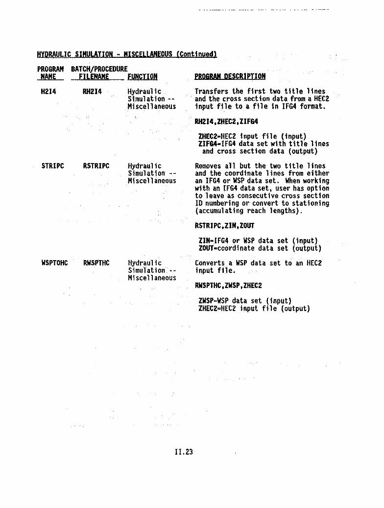
PROGRAM DESCRIPTION
HYDRAULIC SIMULATION " MISCELlANEOUS (Continued>
PROGRAM BATCH/PROCEDUREHAHE FILENAME F~TIO"
H214
STRIPC
WSPTOHC
RH2I4
RSTRIPC
RWSPTHC
HydraulicSimulation -.Hi sce11 aneous
HydraulicSimulationMiscellaneous
HydraulicSimulationHi scellaneous
Transfers the first two title linesand the cross section data from a HEC2input file to a file In IFG4 format.
RH2I4.ZHEC2.lIFG4
lHEC2-HEC2 input file (input)lIFG4-IFG4 data set with title lines
and cross section data (output)
Removes all but the two title linesand the coordinate lines from eitheran IFG4 or WSP data set. When workingwi th an IFG4 data set, user has opt ionto leave as consecutive cross section10 numbering or convert to stationing(accumulating reach lengths).
RSTRIPC.ZIH.ZOUT
llH-IFG4 or WSP data set (input)lOUT-coordinate data set (output)
Converts a WSP data set to an HEezinput file.
RWSPTHC,ZWSP,ZHEC2
ZWSP-WSP data set (input)ZHEC2=HECZ Input file (output)
II .23

ADOCV Program
I. INTRODUCTION
The ADDCY. progtam adds CAL and ·VEl lines to an existing IFG4 data set.An IOC and/or a QARD line with no values, is also added if they do not exist inthe data set. The CAL/VEl data is read from a free-formatted file created withan editor. Refer to Appendix Afar file format for the free-formatted ADDCV fileor type INFOACY for on-line information. Appendix A al so contains a samplefree-formatted input file to ADOCV.
II. RUNNING ADDCV
RAODCY,ZIN,ZIFG4,IJFG4N
ZJN-free-formatted CAl/VEL data file (input)ZJFG4-IFG4 data set in which to add CAL and VEL lines (input)ZIF64N-new IFG4 data set with CAL and VEL lines added (output)
11.24 Program ADDCV

CAlCF4 Program
I. INTRODUCTION
The CAlCF4 program uses Manning's equation at each .cr()ss secti()n t()calculate a water transport parameter (WTP) f()r each water surface elevation inan IFG4 data s..et. It als() devel()ps p()wer relationsh.ips between. WTP's; area .andmaximum depth; and discharge and width, vel()city, and average.depth.
II. RUNNING CAlCF4
RCAlCF4,ZIFG4,ZOUT
ZIFG4~IFG4 data set (input)ZOUT=CAlCF4 results (output)
Figure 11.4 contains sample output from the CAlCF4 program.
11.25 Program CALCF4

88/09/07.09.34.20.
UPPER SALMON RIVER, NEAR STANLEY, IDAHOSAMPLE IFG4 DATA SET
PROGRAM - CAlCF.PAGE - I
CROSS SECTION 10 IS 0.00
REACH LENGTH ooWNSTREAK IS 0.00 WEIGHT ON SECTION IS 0.30STAGE OF ZERO FLOW IS 97.20 GIVEN SLOPE IS 0.02667000
COORDINATE DATA FLOWS - THERE ARE 30 POINTS
DISTANCE O. 2. 4. 4. 5. 8. 12. 14. 16. 16.ELEVATION 101.30 100.70 99.80 98.60 91.10 91.30 97.60 91.90 97.60 97.10
DISTANCE 18. 20. 22. 24. 26. 26. 30. 32. 33. 34.ELEVATION 91.50 97.40 97.30 97.20 97.30 97.50 97.40 97.10 97.60 91.60
DISTANCE 35. 36. 31. 39. 44. 53. 62. 70. 78. 81.ELEVATION 97.10 97.70 97.10 97.90 98.l0 98.80 99.00 98.50 99.00 99.50
DISCHARGE WSL AREA VELOCITY FN AVE DEPTH MAX DEPTH WIDTH WTP
21.80 97.86 11.32 1.93 0.58 0.34 0.68 32.90 3.9412.60 91.16 8.15 1.55 0.53 0.27 0.58 30.48 3.741.90 91.65 5.09 1.55 cO.59 0.21 0.45 24.05 4.38
REGRESSION OF WTP WITH OTHER VARIABLES
XVAR A B STO ERROR AVE ERROR
DISCHARGE 0.5170£+01 -0.099 0.039 4.906DMAX 0.3352E+Ol -0.301 0.035 4.353DAVE 0.3035E+01 -0.213 0.038 4.816
NY RADIUS 0.3027E+Ol -0.214 0.038 4.816
WTP • A• (XVAR) •• B
REGRESSION OF AREA WITH MAXIMUM DEPTH
MAX DEPTH 0.27I1E+D2 2.090 0.005 0.627
AREA = A• (DMAX) .. B
REGRESSION OF DISCHARGE wiTH OTHER VARIABLES
YVM A B STO ERROR AVE ERROR
WIDTH 0.1327E+02 0.304 0.033 4.096VELOCITY 0.9528E+00 0.218 0.036 4.608
DAVE 0.7912E-01 0.478 0.004 0.441
YVAR = A• (DISCHARGE) •• B
ONLY THE DATA FOR THE FIRST CROSS SECTION HAS BEEN INCLUDED IN THIS SAMPLEOUTPUT.
Figure 11.4. Sample output from the CAlCF4 program.
11.26 Program CALCF4
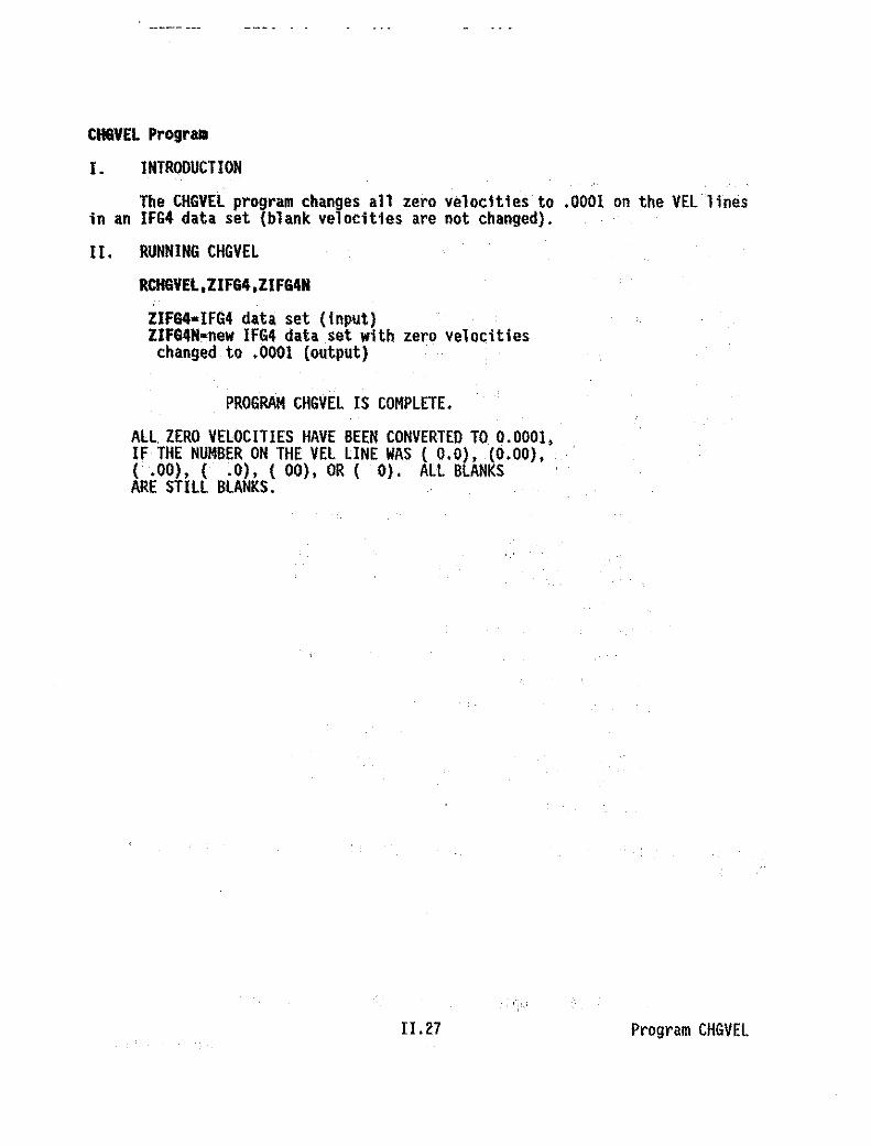
ctl6VEL Prograll
I. INTRODUCTION
The CHGVEl program changes all zero velocities to .0001 on the VEL linesin an IFG4 data set (blank velocities are not changed). .
II. RUNNING CHGVEL
RCHGVEl,ZIFG4,ZIFG4H
ZIFG4-IFG4 data set (input)ZIFG4H-new IFG4 data set with zero velocitieschanged to .0001 (output)
PROGRAM CHGVEL IS COMPLETE.
ALL. ZERO VELOCITIES HAVE BEEN CONVERTED TO 0.0001,IF THE NUMBER ON THE VEL LINE WAS ( 0.0), (0.00),( .00), ( .0), ( 00), OR ( 0). ALL BLANKSARE STILL BLANKS.
11.27 Program CHGVEL

CHSTA P~og~am
I. INTRODUCTION
The CHSTA program changes the cross section ID numbers to stationing inan IFG4 data set. New cross section 10 numbers using stationing are writtenusing one decimal point.
II. RUNNING CHSTA
RCHSTA.ZIFG4.ZIFG4N
ZIFG4-IFG4 data set (Input)ZIFG4N-new IFG4 data set with stationing (output)
11.28 Program CHSTA

CKJ4 Program
I. INTRODUCTION
The CKI4 program checks a complete IFG4 data set for format errors andwrites a summary .of each cross section checked which includes information on:given discharge for point velocities, given stage for point velocities, lowpointon cross section, stage of zero flow, weight on cross section, reach lengthdownstream, and given slope.
II. RUNNING CKI4
RCKI4.ZIFG4.CKOUT
ZIFG4-IFG4 data set (Input)CKOUT-CKI4 results (output)
Refer to Figure 11.5 for sample output from the CKI4 program. This outputwas generated from the Sample IFG4 Data set contained in Appendix A.
III. ERROR MESSAGES
Refer to the IFG4 program description for information on error messages.
11.29 Program CKI4

PROGRAM- CKI4 88/06/01. 10.39.45. PAGE
UPPER SALMON RIVER, NEAR STAHLEY, IOAHOSAMPLE IFG4 OATA SET
IOC VALUES ARE - 0 1 0 0 I 0 0 0 0 0 0 0 1 0 0 0 0 0 I 0000 0 0 0 000 0 0 0 0 0 0 0 0 0 0 0
OTHER OATA LINES PROCEEDING fiRST SET Of CROSS SECTION DATA AME
QARD 8.0QAMD ID.OQAMO 20.0QARD 30.0QARD 40.0QARO 50.0QAMO 60.0QAMO 70.0QAMO 80.0QAMO 90.0QAMO 100.0QAMD 110.0QAMO 120.0OAMO 130.0
Figure 11.5 Sample output from the CKI4 program.
11.30 Program CKI4

PROGRAM- CKI4 83/06/01. 10.39.45. PAGE 2
UPPER SAlMON RIVER, NEAR STANLEY, IDAHOSAMPLE IFG4 DATA SET
CALIBRATION DATA FOR CROSS SECTION 0.00
X Y cilANNEl MANNINGS N POINT VELOClTlESINDEX N DOS 1 2 3
0.0 101.3 3.0 0.000 0 0.00 0.00 0.002.5 100.7 3.0 0.000 0 0.00 0.00 0.004.0 99.8 3:0 0.000 0 0.00 0.00 0.004.3 98.6 3.0 0.000 0 0.00 0.00 0.005.5 97.7 9.2 0.000 I 0.30 0.00 0.007.6 97.3 6.0 0.000 0 0.00 0.00 0.00
11.9 97.6 6.0 0.000 0 0.00 0.00 0.0014.2 97.9 8.2 0.000 a 0.00 0.00 0.0016.2 97.6 8.2 0.000 0 0.00 0.00 0.0016.5 97.7 8.2 0.000 I 0.54 0.00 0.0018.2 97.5 8,2 0.000 I 2.0B 0.00 0.0020.2 97.4 9.0 0.000 I 2.65 0.00 0,0022.2 97.3 9.0 0.000 I 1.91 0.00 0.0024.2 97.2 9.0 0.000 I 2.84 0.00 0.0026.2 97.3 9.0 0.000 1 3.11 0.00 0.002B.2 97.5 9.0 0.000 I 2.59 0.00 0.0030.2 97.4 9.0 0.000 1 I.B7 0.00 0.0032.2 97.7 9.0 0.000 1 2.33 0.00 0.0033.0 97.6 9.0 0.000 I 1.95 0.00 0.0034.2 97.6 9.2 0.000 1 0.56 0.00 0.0035.2 97.7 9.2 0.000 I 0.3B 0.00 0.0036.2 97.7 9.2 0.000 1 1.13 0.00 0.0037.4 97.7 9.2 0.000 0 0.00 0.00 0;0039.1 97.9 10.0 0.000 0 0.00 0.00 0.0043.8 9B.l 10.0 0.000 0 0.00 0.00 0.0053.0 98.6 10.0 0.000 0 0.00 0.00 0.0062.4 99.0 10.0 0.000 0 0.00 0.00 0.0069.9 98.5 8.2 0.000 0 0.00 0.00 0.0078.1 99.0 3.0 0.000 0 0.00 0.00 0.00B7.1 99.5 3.0 0.000 0 0.00 0.00 0.00
GIVEN DISCHARGE 22. 13. 6.GIVEN STAGE 97.66 97.76 97.G5
LOW POINT ON CROSS SECTION 15 - 97.20STAGE OF ZERO FLOW IS - 97.20WEIGHT ON SECTION 15 - 0.30REACH LENGTH DOWNSTREAM IS - 0.00
GIVEN SLOPE 0.02667
SECTIONS OF SAMPLE OUTPUT HAVE BEEN DELETED HERE FOR BREVITY.
$$ JOB COMPLETED • DATA FOR 2 SECTIONS WRITTEN
Figure II.5 (Cond uded)
11.31 Program CKI4
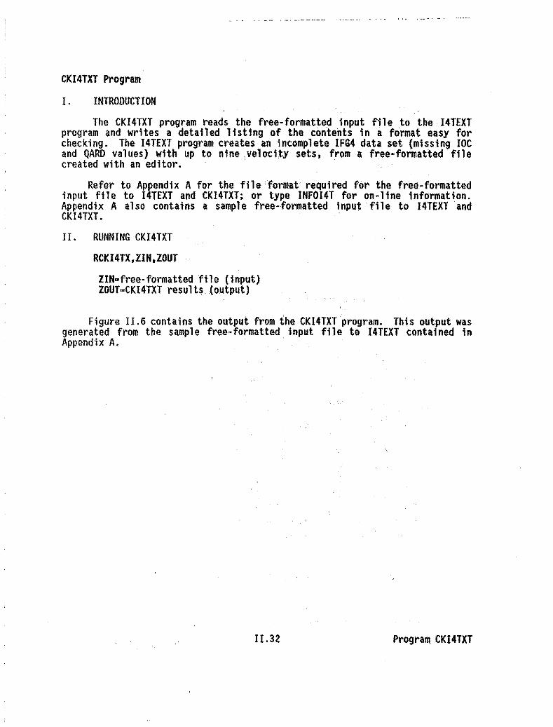
CKI4TXT Program
I. INTRODUCTION
The CKI4TXT program reads the free-formatted input file to the I4TEXTprogram and writes a detailed listing of the contents in a format easy forchecking. The I4TEXT program creates an incomplete IFG4 data set (missing IOCand QARD values) with up to nine velocity sets, from a free-formatted filecreated with an editor.
Refer to Appendix A for the file format required for the free-formattedinput file to I4TEXT and CKI4TXT; or type INFOI4T for on-line information.Appendix A also contains a sample free-formatted Input file to 14TEXT andCKI4TXT.
II. RUNNING CKI.4TXT
RCKI4TX,ZIH,ZOUT
ZIH=free-formatted file (input)ZOUT=CKI4TXT results (output)
Figure 11.6 contains the output from the CKI4TXT program. This output wasgenerated from the sample free-formatted input file to 14TEXT contained inAppendiX A.
11.32 Program CKI4TXT
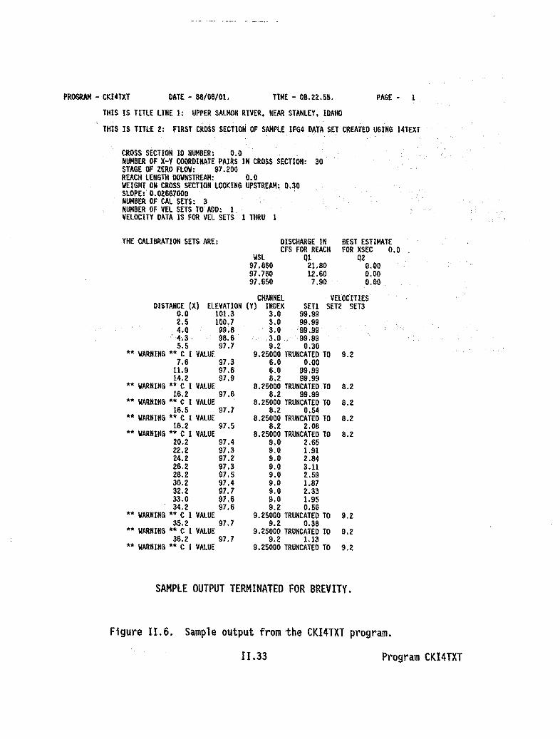
PROGRAM - CKI4TXT DATE - 88/05/01. TIME - 08.22.55. PASE - 1
THIS IS TITLE LINE 1: UPPER SALMON RIVER. NEAR STANLEY. IDAHO
, THIS IS TITLE 2: FIRST CROSS SECTION OF SAMPLE IFG4 DATA SET CREATED USING 14TEXT
CROSS SECTION 10 NUN8ER: 0.0NUM8ER OF X-T COORDINATE PAIRS IN CROSS SECTION: 30STAGE OF ZERO FLOII: 97.200REACH LENGTH OOVNSTREAM: 0.0WEIGHT ON CROSS SECTION LOOKING UPSTREAM: 0.30SLOPE: 0.02887000 'NUMBER OF CAL SETS: 3NUMBER OF VEL SETS TO'AGO: IVELOCITT DATA IS FOR VEL SETS 1 THRU 1
THE CALIBRATION SETS ARE:
WSL97.B5097.76097.650
DISCHARGE INCFS FOR REACH
0121.8012.607.90
8EST ESTIMATEFOR XSEC 0.0
020.000.000.00
CHANNEL VELOCITIESDISTANCE (Xl ELEVATION (Tl INDEX SETI SET2 SET3
0.0 101.3 3.0 99.992.5 100.7 3.0 99.994.0 99.6 3.0 '99.99
, 4.3· 98.6 3.0 99.995.5 97.7 9.2 0.30
•• WARNING •• C I VALUE 9.25000 TRUNCATED TO 9.27.6 97.3 6.0 0.00
11.9 97.6 6.0 99.9914.2 97.9 B.2 99.99
•• WARNING •• C I VALUE B.25000 TRUNCATEO TO B.216.2 97.6 6.2 99.99
•• WARNING •• C I VALUE 8.25000 TRUNCATEO TO 8.216.5 97.7 6.2 0.54
•• WARNING •• C I VALUE 6.25000 TRUNCATEO TO 6.216.2 97.5 6.2 2.08
•• WARNING •• C I VAlUE 6.25000 TRUNCATED TO 6.220.2 97.4 9.0 2.6522.2 97.3 9.0 1.9124.2 97.2 9.0 2.6426.2 97.3 9.0 3.1126.2 97.5 9.0 2.5930.2 97.4 9.0 1.6732.2 97.7 9.0 2.3333.0 91.6 9.0 1.9534.2 97.6 9.2 0.56
•• WARNING •• C I VALUE 9.25000 TRUNCATEO TO 9.235.2 91.1 9.2 0.36
•• WARNING •• C I VALUE 9.25000 TRUNCATED TO 9.236.2 97.7 9.2 1.13
•• WARNING •• C I VALUE 9.25000 TRUNCATEO TO 9.2
SAMPLE OUTPUT TERMINATEO FOR BREVITY.
Figure 11.6. Sample output from ,the CKI4TXT program.
11.33 Program CKI4TXT

CORDIN Program
I. INTRODUCTION
The CORDIN program creates, or adds to, a file of coordinate data and titlelines. An ENDJ and an ENDR line are also created. The CORDIN program is usedin the creation of an WSP data set (it could also be used to create an IFG4 dataset - the ENDR line would have to be deleted).
II. RUNNING CORDIN
RCORDIN,ZCORD,ZCORDIN
ZCORD=coordinate data file with title lines (output)ZCORDIN=coordlnate data file to be added to (optional input)
ENTER TWO TITLE LINES:
Two title lines with up to 80 characters per line may be entered to recordinformation such as the name of the river, section of the river involved,conditions of flow, and any other information describing the data.
THIS PROGRAM CAN CALCULATE THE ELEVATION GIVEN A DATUM AND THEDISTANCE FROM THE DATUM TO THE GROUND SURFACE, IF YOU WANT THISOPTION, ENTER THE DATUM. IF NOT ENTER O.
ENTER CROSS SECTION 10 NUMBER:
ENTER THE NUMBER OF COORDINATE PAIRS FOR CROSS SECTION ---:
ENTER -.. COORDINATE PAIRS FOR CROSS SECTION --- (DISTANCE,ELEVATION):PLEASE PRESS ENTER AFTER EACH PAIR.
When all the coordinate pairs for the cross section are entered -
DO YOU WISH TO ENTER COORDINATE DATA FOR ANOTHERCROSS SECTION? IF SO, ENTER I. IF NOT, ENTER O.
11.34 Program CORDIN

CWSPN Program
I. INTRODUCTION
The CWSPN prQgram adds roughness lines tQ a cOQrdinate data file, Qne valueat each x-v point except tile left-most point. An options (**) Hne. with anoptions off, and an ENOR line are also added if they do not exist. This programis used in the creation of a WSP data set. .
.II. RUNNING CWSPN
RCWSPN,ZIN,ZOUT
ZIN-coordinate data fi.le (input)ZOUT-coordinate data file with roughness, options (**), and
ENOR lines added (output)
ENTER I FOR SAME ROUGHNESS FOR All SECTIONSo OTHERWISE
CHOICE:
If "I" is chosen;
ENTER CONSTANT N:
If "2" 1s chosen:
ENTER CONSTANT N FOR CROSS SECTION ---;
This prompt will be asked for each cross section in the data set.
11.35 Program CWSPN

DELIfSL ProgramI. INTRODUCTION
The DELWSl. pl'ogram deletes WSL lines in an IFG4 data set. WSL 1inescontain the water surface elevations for each flow on the QARD 1ines fol' eachcross section in an IFG4 data set. WSL lines can be added to an IFG4 data setusing the WSEI4. WSEI4D. WSEI4H. or WSEI4S programs; or they can be enteredmanually following the format for 'WSL Lines in an IFG4 Data Set" contained inAppendix A.
II. RUNNING DELWSL
RDELWSL.ZIFG4.ZIFG4N
ZIFG4=IFG4 data set (input)ZIFG4N=new IFG4 data set with WSl lines deleted (output)
[1.36 Program DELWSL
H2EXT Program
I. INTRODUCTION
The H2EXT program extracts specified cross section data frllm the summarytable from HEC2 output. Figure II.S in the HEC2 program section ~ontained inthis chapt~r contains a Sample Summary Table from HEC2 output. .
II. RUNNING H2EXT
RH2EXT,HECOUT,H2EXOUT
HECOUT=output file from HEC2 (input)H2EXOUT=cross section data extracted from the HEC2
summary table (output)
ENTER FIRST AND LAST STATION 10 NUMBERS (SECNO) FOR SETS TO EXTRACT
The SECNO from the summary chart for the first cross section and the lastcross section to be extracted would be entered. All cross sections betweenthe numbers entered will also be extracted.
11.37 Program H2EXT

H214 Program
I. INTRODUCTION
The H2I4 program transfers the first two title lines and the cross sectiondata from a HEC2 input file to a file in 1FG4 format. QARD, NS (if the optionto enter a constant channel index value was not selected), CAL, and VEL linesmust be added to make the resulting file ac()m~lete IFG4data set. These linescan be added using an editor and following the File Format for an IFG4 Data Set"contained in Appendix A, Or by running the following programs:
MODQARD - addsQARD linesADDCV - adds CAL and VEL 1inesAn editor would have to be used to add NS lines.
However, if NS lines were created by H214 by selecting option toenter a constant channel index value, the MODN program could be usedto add or modify the Nvalues. Channel index values would have to bemodified with. an editor.
II. RUNNING H214
RH2I4.ZHEC2.ZIFG4
ZHEC2-HEC2 input file (input)ZIFG4-IFG4 dataset with title lines and cross section data(output)
ENTER 1 FOR NS LINES, 0 OTHERWISE
If "I" was entered:
ENTER CONSTANT CHANNEL INDEX VALUE
The same channel index value would be entered for every cell in thecross section.
Figure 11.7 contains the 1FG4 data set created from an HEC2 input file usingthe H214 program.
11.38 Program H214

TAYLOR RIVER If64, 3 fLOWS Of 162,254,AKO 591 CfS HIGH fLOW SET,NMAXO.IOIFG4 DATA SET CREATED FRON AN HEC2 INPUT FILE USING,THE H2I4 PROGRAMIOC OOOOOOOODOOOOOOOOOOOXSEC 0.0 0.0 0.5
0.0 0.0105.9 5.0100.9 10.0 99.5 15.0 98.8 20.0 98.4 21.997.50.022.0 97.0 22.5 96.8 23.5 98.5 25.096.3 30.0 94.9 3$.0 94.90.0 40.0 95.5 45.0 95.3 50.0 95.2 55.0 95.7 60.0 95.6 65.0 95.50.0 70.0 95.9 75.0 96.0 80.0 95.9 85.095.490.095.5 95:0 95.30.0100.0 95.7105.0 95.5110.0 95.2115.0 95.0120.0 95.3125.0 95.00.0130.094.8135.095.9136.096.8137.696,5140.0 97.3141.5 97,S0.0145;098.5150.099.6155.0100.9160.2103.4 '
KS 0.0 3.0 3.0 3.0 3.0 3.0 3.0KS 0.0 3.0 3.0 3.0 3.0 3.0 3.0K5 0.0 3.0 3.0 3.0 3.0 3.0 3.9KS 0.0 3.0 3.0 3.0 3.0 3.0 3.0KS 0.0 3.0 3.0 3.0 3.0 3.0 3.0KS 0.0 3.0 3.0 3.0 3.0 3.0 3.0KS 0.0 3.0 3.0 3.0 3.0XSEC 67.0 67.0 0.5
67.0 0.0105.4 5.0102.3 10.0100.0 13.097.8 13.1 97.5 15.0 97.167.015.697.1 16.596.820.096.025.095.930.096.435.095.867.0 40.095.2 45.0 95.5 50.095.5 55.0 96.1 60.096.2 65.0 96.467.070.096.475.096.580.096.385.096.490.097.095.095.967.0100.095.5105.0 95.01l0.0 95.0U5.0 95.3120.0 97.1l25.0 95:967.0130.095.6135.095.6138.496.5139.5 96.6140.0 97.0142.6 97.567.0145.098.4150.099.7155.0101.4160.0102.5162.9103.9
KS 87.0 3.0 3.0 3.0 3.0 3.0 3.0K5 67.0 3.0 3.0 3.0 3.0 3.0 3.0K5 67.0 3.0 3.0 3.0 3.0 3.0 3.0KS 67.0 3.0 3.0 3.0 3.0 3.0 3.0KS 67.0 3.0 3.0 3.0 3.0 3.0 3.0KS 67.0 3.0 3.0 3.0 3.0 3.0 3.0KS 67.0 3.0 3.0 3.0 3.0 3.0XSEC 132.0 65.0 0.5
132.0 0.0105.2 5.0101.5 9.798.1 10.0'97.9 11.6 97.3 13.597.0'132.0 15.0 95.3 20.0 94.7 25.0 95.0 30.0 95.5 35.0 95.3 40.0 95.7132.045.095.8'50.096.055.095.760.095.9 65.095.7 70.09$.1132.0 75.095;5 80.0 95.5 85.0 95.5 90.0 95.6 95.0 96.1100.0 95.9132.0105.0 95.3110.0 95.0115.0 94.7120.0 95.0125.0 96.1130.0 96.7132.0131.997.2133.497.3135.097.6138.2 98.1140.0 99.0145.0 99.7132.0150.0100.5155.0101.0160.0103.5161.4104.3
KS 132.0 3.0 3.0 3.0 3.03.0 3.0KS 132.0 3.0 3.0 3.0 3.0 3.0 3.0KS 132.0 3.0 3.0 3.0 3.0 3.0 3.0KS 132.0 3.0 3.0 3.0 3.0 3.0 3.0KS 132.0 3.0 3.0 3.0 3.0 3.0 3.0KS 132.0 3.0 3.0 3.0 3.0 3.0 3.0KS 132.0 3.0 3.0 3.0 3.0EKOJ
Figure 11.7.program.
IFG4 data set created from a HEC2 input fil e us i og the H214
11.39 Program H214

HEC2 Program
I. INTRODUCTION
The HEC2 program is not part of PHABSIM, but it can be used to determinewater surface elevations. The HEC2 program uses step backwater calculations todetermine water surface elevations.
The HEC2 program was developed, and is supported, by the HydrologicEngineering Center of the U.S. Army Corps of Engineers. Refer to the "HEC-2Water Surface Profile Users Manual" for program documentation.
II. RUNNING HEC2
The Aquatic Systems Branch does not maintain a version ofHEC2 for publicuse. In order to run HEC2, the user must have independent access to thepackage"
There are both mainframe and microcomputer versions of HEC2 available.The Hydrologic Engineering Center has also developed options not describedor used in this manual but are useful when doing instream flow studies.
For information on HEC2, Federal agencies should contact the HydrologicEngineering Center; others should contact the revel ant private group or'university.
The following four programs have been developed by the Aquatic SystemsBranch for use with HEC2. See the individual program documentation for moreinformation on these programs.
WSPTOHC - Converts a WSP data set to a HEC2 input file.H2I4 - Transfers the first two title lines and cross section data
from a HEC2 input file to a file in IFG4 format.H2EXT - Extracts specified cross section data from the summary
table from HEC2 output.WSEI4H - Reads water surface elevations and discharges from a HEC2
output file and adds or replaces the QARO and WSl lines inan IFG4 data set.
When running HEC2, the code numbers contained in Table 11.1 must be selectedon Job Control Parameter Card 3 (J3) in order to generate the "Summary Printout"in the right format to be read by H2EXT and WSEI4H. Figure 11.8 contains aSample Summary Table from HEC2 output.
II .40 Program HEC2

Table 11.1
Code numbers that must be selected on the Job Control Parameter Card 3 (J3)in order to generate the "Summary Printout" in the right format to be read byH2EXT and WSEI4H.
Codef1jlg Number Description
1 38 Cross section identification number2 43 Discharge3 1 Computed water surface elevation4 4 Cross section width at calculated water surface elevation5 5 Slope of the energy grade line for the current section
(times 10,000)6 6 Travel time from the first cross section to the
present cross section7 7 Cumulative volume of water in the stream from the first
cross section in acre-feet8 8 Depth of flow9 10 Mean velocity head across the entire cross section
10 .81 ank
HAl Program HEC2
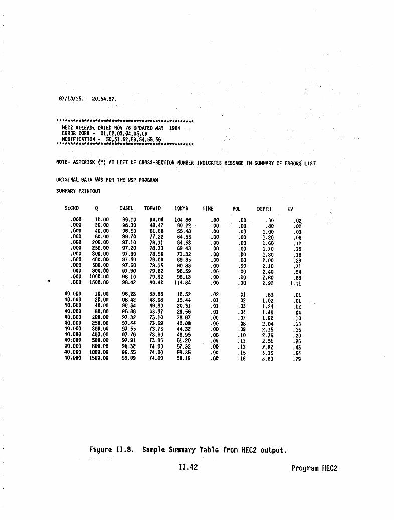
81/10/15. 20.54.57.
****.w*******************.********~***********.*_*
HEe2 RELEASE DATEO HOV 76 UPDATED HAY 1984ERROR CORR - 01.02.03.04.05.06MODIFICATION - 50;51.52.53,54.55.56
**************************************************
NOTE- ASTERISK (*) AT LEFT OF CROSS-SECTION NUMOER INDICATES KESSAGE IN SUMMARY OF ERRORS liST
ORIGINAL DATA liAS FOR TKE IISP PROGRAM
SUHHARY PRINTOUT
SECNO Q CIISEL TQPIlIO IOK*S TIME VOL OEPTH MY
.000 10.00 96.l0 34.00 104.86 .00 .00 .60 .02
.000 20.00 96.30 48.41 60.22 .00 .00 .80 .02
.000 40.00 96.50 51.50 55.48 .00 .00 1.00 .03
.000 80.00 96.70 11.22 64.53 .00 .00 1.20 .06
.000 200.00 97.10 78.11 64.53 .00 .00 1.50 .12
.000 250.00 97.20 18.33 69.43 .00 .00 1.10 .15
.000 300.00 97.30 78.56 71.32 .00 .00 \.80 .10
.000 400.00 97.50 79.00 69.85 .00 .00 2.00 .23
.000 500.00 97.60 79.15 80.83 .00 .00 2.10 .31
.000 800.00 97.90 19.62 96.59 .00 .00 2.40 .54
.000 1000.00 98.10 79.92 98.13 .00 .00 2.60 .68* .000 1500.00 98.42 80.42 114.84 .00 .00 2.92 \.11
40.000 10.00 96,23 38.66 12.52 .02 .01 .83 .0140.000 20.00 96.42 43.08 15.44 .01 .02 1.02 .0\40.000 40.00 96.64 49.30 20.5\ .01 .03 1.24 .0240.000 80.00 96.86 63.31 26.56 .0\ .04 1.46 .0440.000 200.00 97.32 73.10 38.87 .00 .07 1.92 .1040.000 250.00 97.44 73.69 42.08 .00 .08 2.04 .1340.000 300.00 97.55 13.73 44.32 .00 .00 2.15 .\540.000 400.00 91.16 13.80 46.95 .00 .10 2.36 .2040.000 500.00 97.91 13.86 5\.20 .00 .11 2.51 .2640.000 800.00 98.32 74.00 51.32 .00 .13 2.92 .4340.000 1000.00 98.55 74.00 59.35 .00 .15 3.15 .5440.000 1500.00 99.00 74.00 58.19 .00 .18 3.69 .79
Figure 11.8. Sample Summary Table from HEe2 output.
II .42 Program HEe2

14TEXT Program
I. INTRODUCTION
The I4TEXT program creates an incomplete IFG4 data set (missing IOC andQARD values) with up to nine velocity sets, from a free-formatted file createdwith an editor. The CKI4TXT program is run to check the free-formatted filebefore the 14TEXT program is run. CKI4TXT writes a detailed listing of thecontents in a format easy for checking.
The MODIOC program could be run on the IFG4 data set created by 14TEXT toadd IOC values; and the MODQARD program could be run to add QARD values.
Refer to Appendix A for the file format for the free-formatted input filefor 14TEXT and CKI4TXT; or type INFOl4T for on-line information. Appendix A.alsocontains a sample free-formatted input file to I4TEXT.
II. RUNNING 14TEXT
RI4TEXT,ZIN,ZIFG4
ZIN=free-formatted file (input)ZIFG4=IFG4 data set (output)
11.43 Program 14TEXT

14TI1SQ Program
I. INTRODUCTION
The I4TMSQ program converts an IFG4 data set to a MANSQ data set, with oneflow per cross section entered on the CALQ line.
II. RUNNING I4TMSQ
RI4TMSQ.ZIFG4.ZMANSQ
ZIFG4=IFG4 data set (input)ZMANSQ~MANSQ data set (output)
The IFG4 data set title lines wHl be displayed.
DO YOU WANT TO CHANGE THE TITLE? YIN
FOR CROSS SECTION ---
ENTER THE WATER SURFACE ELEVATION ON CALQ LINE:
ENTER THE FLOW ON CALQ LINE:
ENTER BETA COEFfICIENT:
The above series of prompts will appear for each cross section inthe IFG4 data set.
Refer to Appendix Afor the "MANSQ Data Set Format" and a sample MANSQ dataset.
II.44 Program I4TMSQ
....••• _.... _•. - --_.' -- _. - _.. __.. _-<.
14VAF Program
I. INTRODUCTION
The 14VAF program plots or summarizes and plots the velocity adjustmentfactors file (ZVAFF) created when IOC(13)=1 in IFG4.
II. RUNNING I4VAF
RI4VAF,ZVAFF,ZOUT
ZVAFF=velocity adjustment factor file from IFG4 (input)ZOUT=I4VAF results (output).
On the microcomputer, graphs may be printed to the screen or to the outputfile using character graphics (132 characters per line format). In orderto use screen graphics, the computer must have a Color Graphics Adaptor(CGA) or compatible graphics card. When using screen graphics, notes .arewritten to the output file in the positions where the graphs would havebeen placed had they been written using character graphics.
SELECT DESIRED OUTPUT1) PLOT ZVAFF FILE2) PRINT SUMMARY STATISTICS AND PLOT ZVAFF FILE
CHOICE:
Figure II. 9 contains sample output from the I4VAF program. This figurecontains the summary statistics and the plot generated by selecting Option "2"above. The ZVAFF file was generated by running IFG4 on the Sample IFG4 Data Setin Appendix Awith IOC(13)=I.
Velocity Adjustment Factors for flows less than the calibration flows arelikely to be less than one. Velocity Adjustment Factors for flows greater thanthe calibration flows are likely to be greater than one.
II,4S Program 14VAF
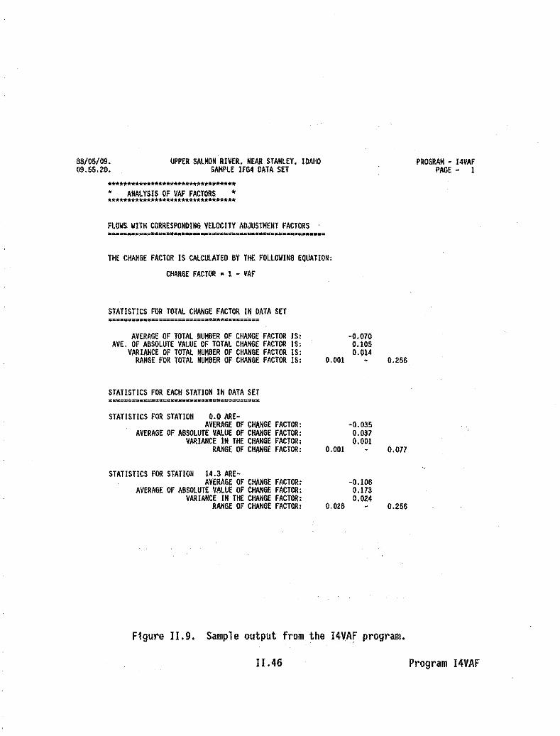
88/05/09.09.55.20.
UPPER SALMON RIVER. NEAR STANLEY. IDAHOSAMPLE IFG4 DATA SET
PROGRAM - 14VAFPAGE - 1
**.****************************~
• ANALYSIS OF VAF FACTORS •*~*ww************~******.*****~
FLOWS WITH CORRESPONDING VELOCITY ADJUSTMENT FACTORS
THE CHANGE FACTOR IS CALCULATED 8Y THE FOLLOwiNG EQUATION:
CHANGE FACTOR • 1 - VAF
STATISTICS FOR TOTAL CHANGE FACTOR IN DATA SET~~=.w.w_.~.~==============.· •••~~=====
AVERAGE OF TOTAL NUMBER OF CHANGE FACTOR IS -0.070AVE. OF ABSOLUTE VALUE OF TOTAL CHANGE FACTOR IS 0.10S
VARIANCE OF TOTAL NUMBER OF CHANGE FACTOR IS 0.014RANGE FOR TOTAL NUMBER OF CHANGE FACTOR IS 0.001 0.256
STATISTICS FOR EACH STATION IN DATA SET~.*====.~======c~ ••••••••••~~=~======u~STATISTICS FOR STATION 0.0 ARE-
AVERAGE Of CHANGE FACTOR -0.035AVERAGE OF ABSOLUTE VALUE OF CHANGE FACTOR 0.037
VARIANCE IN THE CHANGE FACTOR 0.001RANGE OF CHAN6€ FACTOR 0.001 0.077
STATISTICS FOR STATION 14.3 ARE-AVERAGE OF CHANGE FACTOR -0.106
AVERAGE OF ABSOLUTE VALUE OF CHANGE FACTOR 0.173VARIANCE IN THE CHANGE FACTOR 0.024
RANGE OF CHANGE FACTOR 0.028 0.256
Figure 11.9. Sample output from the I4VAF program.
11.46 Program I4VAF
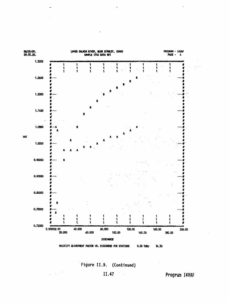
/JIWi/f9. I.Fl'Sl &IllDl RI1IEII, EM STNlEr, I\WI) _'I~VN'
09.55.20. _ IIll4 MTA lI!T IWlE • 4
T.3aXlI 1 T 1 I I 1 1 1 II 1 T 1 1 1 1 1 1 II 1 T I 1 1 T 1 1 II I
l.llSllO I··" B ····1I B II 8 II 8 II 8 ,I.
1.2000 ,.... 8 ····11II III 8 III III 8 1/
1.1400 I ..·· •• ..1II. 8 1/I I1/ II I
l.lSI) ""A A- •• ..1I A A- 1/I A I
VAl , A A 1/I 8 A I
l.lWl I···· A ....,1/ A A- II A- A- A- ,I ItI I
0.%000 1/.... B ····It, ,, ItI 1/tI I
0.900)) ,.... ....,tI 1/1/ I, ,tI I
0.S4000 ,.... ....,, ,, ,, 8 1/1/ 1/
0.l8:XXl 1/.... ..··1, B I, 1 1 1 1 1 1 1 1 1 ,, 1 1 1 1 1 T 1 1 1 ,I 1 1 1 1 1 1 1 T 1 I
O.l2OOOO.lJO(XXl''01 4O.00l OO.OOl 1211.00 lro.oo 100.00
2/l.00l ro.OOl 100.00 ~.OO 18l.ooOISClWlOE
\ROCIIY Jl).u$llfiIl! FACTQl \'S. OISClWlOE RR STA-TlCllS 0.00 TlR) 14.30
Figure II .9. (Continued)
11.47 Program I4VAF

8B/05/09. UPP<R SALMON RIVER, NEAR STANLEY, IDAHO PROGRAM • 14VAF09.55.Z0. SANPLE IF64 DATA SET PAGE· 5
STATISTICS FOR EACH FLO\I IN DATA sn••--=-=~~••~=~==.=.=~W.R~~~U.ft~==.~=
STATISTICS FOR FLOW 8.000 ARE -AVERAGE OF CHANGE FACTOR: 0.078
AVERAGE OF ABSOLUTE VALUE OF CHANGE FACTOR: 0.155VARIANCE IN CHANGE FACTOR: 0.OZ4
RANGE OF CHANGE FACTOR: 0.077 0.Z33
STATISTICS FOR FLOW 10.000 ARE -AVERAGE OF CHANGE FACTOR: 0.063
AVERAGE OF ABSOLUTE VALUE OF CHANGE FACTOR: 0.129VARIANCE IN CHANGE FACTOR: 0.017
RANGE OF CHANGE FACTOR: 0.065 0.192
STATISTICS FOR FLOW 20.000 ARE -AVERAGE OF CHANGE FACTOR: 0.023
AVERAGE OF ABSOLUTE VAlUE OF CHANGE FACTOR: 0.023VARIANCE IN CHMGE FACTOR: 0.001
RANGE OF CHANGE FACTOR: 0.001 0.048
STATISTICS FOR FLOW 30.000 ARE -AVERAGE OF CHANGE FACTOR: -0.009
AVERAGE OF ABSOLUTE VAlUE OF CHANGE FACTOR: 0.019VARIANCE IN CHANGE FACTOR: 0.000
RANGE OF CHANGE FACTOR: 0.009 0.02B
STATISTICS FOR FLOW 40.000 ARE -AVERAGE OF CHANGE FACTOR: -0.03B
AVERAGE OF ABSOLUTE VALUE OF CHANGE FACTOR: 0.042VARIANCE IN CHANGE FACTOR: 0.002
RANGE OF CHANGE FACTOR: 0.004 O.OBI
STATISTICS FOR FLOW 50.000 ARE -AVERAGE OF CHANGE FACTOR: -0.OB3
AVERAGE OF ABSOLUTE VALUE OF CHANGE FACTOR: 0.063VARIANCE IN CHANGE FACTOR: 0.004
RANGE OF CHANGE FACTOR: 0.004 0.123
STATISTICS FOR FLOW 60.000 ARE -AVERAGE OF CHANGE FACTOR: -0.083
AVERAGE OF A8S0LUTE VALUE OF CHANGE FACTOR: 0.083VARIANCE IN CHANGE FACTOR: 0.005
RANGE OF CHANGE FACTOR: 0.012 0.154
Figure 11.9. (Concluded)
11.48 Program 14VAF

.. - .. _.. - -. -.. .. _.... -- .
I4VCE Program
I. INTRODUCTION
The I4VCE program plots or summarizes and plots the velocity calibrationerrors file (ZVCEF) created when IOC(IO)"l in IFG4.
II. RUNNING 14VCE
RI4VCE,ZVCEF,ZOUT
ZVCEF~velocity calibration errors file from IFG4 (input)ZOUT-I4VCE results (output). Graphs are written usingcharacter graphics in a 132 characters per line format.
SELECT DESIRED OUTPUT1) PLOT ZVCEF FILE .2) PRINT SUMMARY STATISTICS AND PLOT ZVCEF FILE
CHOICE:
Figure 11.10 contains sample output from the I4VCE program. This figurecontains the calibration errors and the plot generated by selecting Option "2"above.
III. ERROR MESSAGES
***NOTE***THERE IS ONLY ONE ERROR VALUE PER STATION IN DATA SET• THEREFORE STATISTICAL CALCULATIONS ARE OBSOLETE.**ERROR** EMPTY VCE FILE (OR EOF) - TRY AGAIN
There must be multiple non-blank velocity sets in the IFG4 data set inorder for the program to develop regression line'S to calculate the measuredflow for each cross section versus the user supplying the measured flowon the CAL line for each cross section. Therefore, a ZVCEF file could notbe generated using the Sample IFG4 Oata Se~ in Appendix A, as there is onlyone non-blank velocity set.
H.49 Program I4VCE

8IV06/3O. WKlI RII'EIl, NEll '/lllK, UImJI)Y fl.QllOla.. lUtBl _ (alUII) _·14'ICE00.47.55. lOB! WIlM 9:liIlI/liIl-4/Z'1HI7 _ lXl.IHI \nlt!TY (JI3lE,616.4 10 672,0.9) !WE • 2
0.J(jXQ~ 1 1 1 1 1 * 1 1 1 1 ~
~ 1 1 1 ., 1 * 1 1 . 1 1 ~• 1 1 1 1 1 1 1 1 1 •• •0.27000 ..... * .....• * ~• •• * •• * •0.10::00 ..... ....~• * •~ •• * * •• * * •O.OIXXKIH~ ..... * * ....~~ • * * * *.~* * * * •~* * • * *.." "* * " *.,...". * * • •..·ItIt" • • * * •." • * * * *.
'ICE ~* * *.• * * *.·9.00xtt·(l2 ".... * * * ..•.,
~* * ~• * •• * •• * * */1'0.10::00 ..... ....•
• •It ItIt * •It * It
'0.27000 ".... • •••••It *', ,,
*'~ * •,0.3600) ,.... ....,1/ ,, ItIt •It It
'0.45000 1/•••• ....~It ~It 1 1 1 1 1 1 1 1 1 ~
It 1 1 1 ., 1 1 1 1 1 It~ 1 1 1 1 1 1 1 1 , It
,0.5«(090.001 210.00 450.00 610.00 1110.00 090.00
'181.00 311;1.00 540.00 720.00 900.00
01_
PlOT (1! \£UlCIlY rAI._rrlJl EllIOlS
Figure 11.10. Sample output from the 14VCE program.
H.50 Program 14VCE

88/06/30.88.47 .55.
SALMON RIVER, NEW YORK, UNSTEADY FLOW HODEL, SUMMER 1986 (COUNM) PROGRAM - 14VCELOWER DUNBAR S056M/SIH/NI-S7 MEAN CDLUMIl VELOCITY (NOT£,648.4 TO 87~.9.9) PAGE - 3
AVERAGE OF TOTAL NUM8ER OF ERRORS IS: -0.007AVE. OF A8S0LUTE VAlUE OF TOTAl ERRORS IS: 0.079
STAND. OEV. OF TOTAl NUMBER OF ERRORS IS: O.lllRANGE FOR TOTAl HUMBER OF ERRORS IS: -0.495 0.349
STATISTICS FOR STATION 56.0 ARE-AVERAGE OF ERRORS: -0.007
AVERAGE OF ABSOLUTE VALUE OF ERRORS: 0.083STARO. DEV. IN THE ERRORS: 0.119
RANGE OF ERRORS: -0.3lS 0.349
STATISTICS FOR STATION 58.D ARE-AVERAGE OF ERRORS: -0.007
AVERAGE OF ABSOLUTE VALUE OF ERRORS: 0.076STANO. OEV. IN THE ERRORS: 0.124
RANGE OF ERRORS: -0.495 0.3l9
Figure II.lO. (Concluded)
11.51 Program 14VCE

IFG4 Program
I. INTRODUCTION
The IFG4 program uses a stage-discharge relationship to determine watersurface elevations unless they are supplied in the data set. When using thestage-discharge relationship, each cross section is treated independently of allothers in the dataset. The velocities are determined using techniques basedon Manning's equation.
The IFG4 hydraulic simulation model predicts depth of flow and mean columnvelocities across the stream as a function of discharge. The purpose of theprogram is to develop the depth and velocity data required by the habitatsimulation programs. Given the appropriate streamflow data. it is possible toregress discharge with water surface elevation. and discharge with mean columnvelocity, using a log-log fit with discharge as the independent variable. Thedistribution of depth across the stream is obtained implicitly within the programby subtracting the known ground/streambed elevations from the predicted watersurface elevation at the cross section.
The IFG4 program is capable of making water surface elevation and velocitypredictions for up to 100 flows in a single run. However. When the lFG4 programis used in conjunction with the habitat simulation programs. the limit is 30flows.
As noted above, the 1FG4 model is based on the empirical assumption thatwater surface elevation and velocity exhibit a log-log linear relationship toflow. For a valid relationship between velocity and flow to be obtained,it isimperative that all sets of velocity measurements for all measured flows be madewith respect to a common set of verticals. Generally, closer spacing ofverticals is required in the middle of the channel for accurate simulation oflow flows.
The 1FG4 program defines a cell as the region one-halfway between two setsof adjacent verticals. A vertical is a measurement point specified as the X(distance from the head stake) coordinate values. All references to the cellare then made to the vertical. Note that this definition of a cross-sectionalcell is different than that used in the HABTAT program. When processing iscomplete, 1FG4 passes simulated velocity and depth information to HABTATin theform used there.
Refer to Figure ILl for a flowchart of the various methods available tocreate an IfG4 data set. Refer to Appendex A for "IFG4 Data Set File Format"for information on what each line contains and instructions for entering data.Appendix A also contains a sample 1FG4 data set.
Table 11.2 describes the options available in the 1FG4 program.
II. 52 Program IFG4

S
Table 11.2. Options in the IFG4 Program.
OPTION ACTION
1 Prints the numerical details of tha computed velcx:itles and wAte.r $utf~ce e18vat1onsfor each ~tmulilted
dl.c~rge. Recommend setting to zero (0) for production run' and one (1) forcallbraticn runs. Ifa reCord of the velocities and VSL's used In the production run. i. desired, use the related optionsIn HABTAT. for calibration runs, the flows on the QARD lines should be the same as on the CAL ltne.if all the "best estimates" of flows at each cross SeGtton are the same. otherwise use a ,setreptesentat 1ve of the- measured flows.
o =Do not print computational details.I • Print computational detail•.
2 Prints the numerical details of theoaHbration procedure and gent!rat.s output .hich help. spot erroroand indloates additional parameter adjustments. Recommend setting to one (1).
0- Do not print calibration detail$.1 =Print calibration details.
3 Generates a plot of the cross section coordinate points. An alternative 1s to run the REVr4~progt~m.Recommend setting to zaro (0).
o ~ Do not plot cross sections.1 • Plot cross sect tons.
,4 Generates plots of the points of the stage-discharge rating curve based on log transformat ton.
Reoommend running the REVI4 program to look at the stage'dlscharge relatlon.hlp prior to running theIFG4 pr<>;jra1J\. If only one set of CAL-VEL data Is In the data set, this option ....t baset to zero (Dl.
o ~ 00 not plot rating curve.t ~ Pl~t rating CUrve.
Controls .the discharge used In the collbrotlon(s~. Ifles the stage-discharge an~ velocitY-dischargerelotlonships In relation to slmulotod dlsohorges). set IOC(5).0 If IOC(8)-e. Recommend setting tozero ..0.... ..
o ~ Discharge calculated ~oreAch cross section is usedin the calibration of y*aQand in the stage-discharge relationship If IOC(8)'0.
1 ~ Stage-discharge relationship and velocity dischargerelationships are determined using the first dischargeentered on the CAL lines.
6 A11"". 0 correction In stage If the Velocity Adjustment Factor Is bayond speo If Ie bounds. Recommendsetting to zero (0) as it is more effective to set IOC(S)-! and input the water $u~face elevatioos~
o• Will adjust velocities only to make the meosureddischarge equal to the calculoted discharge.
I =VIII all.. a correction In .tage If the VelocityAdjustment Factor is 1ess t~n 0.90 or greater thanl.10.
7 A11..s user to specify the Stoge of Zero Fl"" (SZF) - the limiting elevation in regard to flow. Thiscan be represented by the lowest point in thecrO$s section or the limiting elevation of downstreamcross sections. Reoommend entering the stage of zero flow on the XSEC line and setting tht$ optionto zero (0). .
o = Read stage of zero flow from XSEC line.1 = Set stage of zero flow to ~ero.
11.53 Program IFG4

Table 11.2 (Continued)OPTION ACTION
8 Defines the computatIon technIque. of the velocity/dlsoharge and stage/dlaoharge relatlon.hips.
0- Use ratIng .urve.ba.ed on flow seleoted by IOC(5) to·oaloulate .tage for the flows entered on the QARDlines:.
1 a Water surface elevation is supplied on WSl lines foreaoh flow entered on the QARO lines.
2 =Stage i. cal.ulated u.lng two .tage-disohargerelatIonships. The flr.t stage-disoharge relationshipuses the water surface elevations entered On the CAtline. and the flr.t flow entered on the CAL lines. Thesecond stage-dlsoharge relatIonshIp uses the watersurface elevdions entetedon the CAL l1nes; and, thedl.oharges oaloulateduslng the given .eloolties Or the.econd flow on the CAL llne If the velooltle. are notgiven. for eeoh flow e.tored on the QARD Hne•• thewater surface elevation is calculated using the firstrelationship. This water surfaoeelevatton 'S ~sed todetermine a discharge using the second,relattonsh1p; thisdlsoherge Is used In tha water (mass) .balanoe oaloulation••The velocity vs. discharge relationships are based on thedischarge calculated ustng the velocities on the VEL lines.
If .elooltles are all blank (flow oaloulated based onVEL llne.-OJ, then the .econd flow on the CAL line I.used the same way n the discharges calculated fromthe vel..ltle. on the VEL lIne.. In thIs oa'e, the .econddischarge on the CAL line must b. given.
SpecIfically, If IOC(8)-2, there HUSI be either non-blankveloolty data OR two flow. on the CAl Jine••
NOTE: Option 5 mu.t be off to allow this option tofunotlon correctly; the ad.antages of IOC(81-2.re lo.t If IOC(Sj-I.
9 ProVides for evaluation of negative velocities. When Qpt10nis off. only the call with the negativBvelocity will be evaluated as a semi-log fit. When option is on, one negatIve velooity will foroe theentl.. oro.s ...tlon to be e.aluated by a ....I-log fit. The relatIonshIp. developed In the oallbrationphase are thus forced to be semi-log relatIonshIp. and the simulatIon .teps a.. performad u.ing tho••functIon.. Rsc""""nd .etting to 'ero (0).
o - VIlen a negative veloolly I. found, a seml-l09equation I. used to oalibrate that oell ONLY.
I - VIlen a negative veloolty I. found. all oell. in thecrOs....tlon .re oallbrated using a .eml-log equatIon.
10 Vrltes ZYCEF fIle containing. summary of the Velocity CalIbration Error. whloh are (V - oQ**B) foreaoh oell and the error faotors for velooity. Resulto are only obtaIned If the program I. using~ltfple non·blank velocity sets to develop regress10n ltnes to calculate the measured flow for ebohcross section versus the user supplying the me«!ured flow on the CAL line-for each Cross section.Rsc.....nd settIng to 'ero (0) for productIon run. and until the model has .uocessfully run onoe. Setto one (I) to check for slgnlfloanoe of the V-Q calibration on .ubsequ.nt oallbratlon run••
o - 00 not .rite ZVCEF file.1 - vrlte ZVCEF file.
11.54 Program 1FG4

Table 11.2 (Continued)OPTION ACTION
11 Applles the veloe tty edjustment fector (VAF). If IOCIll).l, the velocity adjustment wi 11 be bypas.edregardless of which combinstlons of OptlonsS and 8 have been aeleeted. Set IOC(l1)-O if lOC(I.).!.Recommend alway. setting IOC(II).O. Setting IOC(II).1 Is sometimes referred to .s "turning off mas.balencing"•
o c Adjust velocities So the dtacharge calculated using the~'mulated velocities is the sama~s a disoharge enteredon the QARD line.. The adjusting is done using theVelocity Adjustment Factors.
I • Dc not adjust velocities using VAf.
12 Allows user to have the program calculate roughne$s coefficient if roughness values arenotsuppl1ed.or to supply the roughness coefficient for each cell with only one measurement.
o ~ Uses Hon the us ltnes, or calculates H if N onUS line 1~ zerG. .
1 ~ Uses calculated Hfor cells with water. Non US linesfor dry cells for which Nwasiupplied•. and on'estimated N for dry eells whereN was not-supplfed;
13 Writes ZVAFF file containing a sunmary of the Velocity Adjustment Factors. If lOC(l) lIIO, Teconmends.ttlng IOC(13)·1 and checking ZVAFF file for lerge VAF v.lues. Velocity Adjustment Factors for flowsless than the calibration flows are likely to be lass than one. Velocity Adjustment Faotors for flowsgreater than the calibrst10n flows are likely to'begiea~er than one.
o• Do not write ZVAFF file.I • Write ZVAFF file.
14 Controls the use of the coefficient (d) in v~ cQ**d~
o = No control of coefficient d.1 ~ Uses the average coefficient d of the cells wtth at
least three measured velocities ag the coefficient forall cells~with at least one measurement.
2= Uses the average coefficientdwith the eellswtth onlyone velocity measurement, other cells are unchanged.
3 = limits the coefficient d to am3x1mum valu8spectftedby the USer on the BHAXltne.
4 = Uses the average coeff'ctent d for all cells w1th oneor two measure~ YelocH iea.
5 • Uses the average COefficient d for oell$ with onem8&$ured velocity and applies a limit to d(I.e .• 2 and 3 combined).
15 Limits the maximum OR minimum and maximum value of the roughness coefficient (0) used by Hanntng t$
Equation in simulating velocities.
o: No limit on N.1 »·Umit on the maximum OR on th<!' IMximum and .minimum
value of Nlv.lue. supplied on the NMAX line).2 = limit on the maximum value of N and on ~inlmum
if N > 0 (v.lues supplied on tho HMAX line).
11.55 Program IFG4
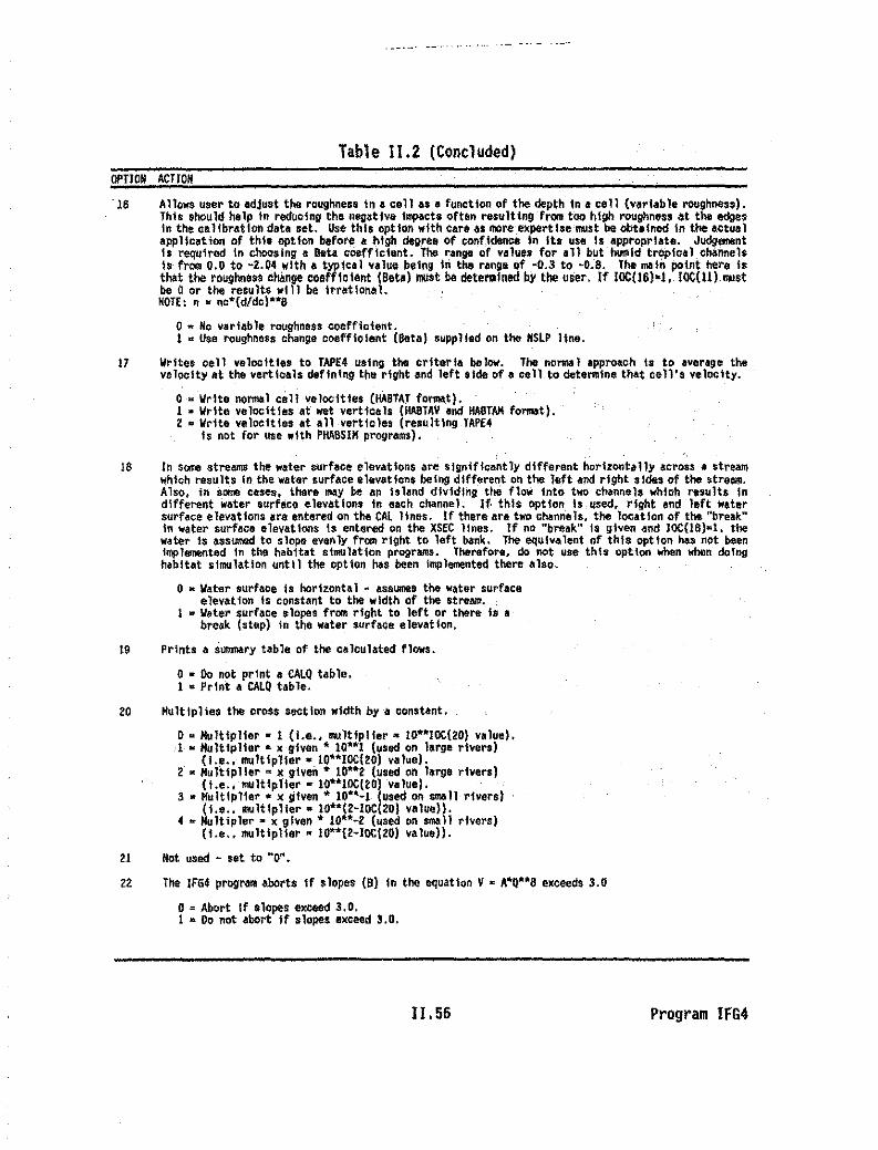
Table 11,2 (Concluded)OPTION ACTION
·16 All""s user to adjust the roughness In a ce11 as a function of the depth in a cell (vorlab1. roughness).This should help in red.olng the negative Ill1I"cts often resulting fr<>m toa high roughn.ss at the edgesIn the o-aHbrat Ion data set. Use- this opt ion with care 4:8 more-expert be must be obtained 1n the eotua 1appHcation of this aption before. a high degree of conf.jdance in Ito us. Is appropriate. Judg....ntIs required in choosing a Beta co.fflcient. The range of va1uu for all but humid trOpical chilnnel,Is frem 0.0 to -Z.04 with a typical value being in the range of .-0.3 to -O.S. The main point here isthat tho raug,,"." oI"noo coefficient (Beta) must be dete....lned by the u,er. If IOCll6N, IOC(llI."",tbe 0 or the results will be Irrational.NOTE: n • nc'{d/de)"S
o to; No variab le roughne-n coefficient.1 • Use roughness chenge coefflolent (Betal supplied on the HSlP line.
17 Writes cell velocities ta TAPE••,I"1l the criteria below. The normal approach is to averag. thevelocity at the verticals defining the right and left 'Ide of. c.ll to det.rmine that cell', v.loclty.
o • Write normal c.ll v.locltie, (ItA8TAT format). .1 • Writ. v.1ocltle, at wet v.rtioels (ItA8TAY and HASTAM format).Z • Writ. ve loc it Ie, at all verticles (resulting lAPE4
Is nat for .se with PHA8SIM progralll1).
18 In some streams the water $urface elevations are Significantly different hortzontal1y 4crOS$ a streamwhich resultstn the water surface elevations belll9 dffferen,t on the TeH and right ,,1des of the $treom.Also. in S~ cases. there ~y bean island dividing the ftO\ll into- two c~nne" wh1Clh results indifferent water surface elevations tn each channel~ If this option 1$ used, right and left w~ter
$urf~ce elevations. are entered on the CAL Hnes. If there are two channels, the location of the "break"in water surface elevations is entt:'rCKf on the XSEC Hnes. If nO "break" Is given and IOCOS)-t. thewater is assumed to slope Q:ven:ly from r1ght to left bank. The equty~lfmt of thts option has not beenimplemented 1n the: hab1tat simulation programs. lherefote~ do not use- thts option when when doinghabltet simulation until the optl.n has been implemented there e1'a.
o M Watet &urface is horizontal R assumes the water surfaceelevation is constant to the width of the stream.
1 w Water surface slopes from right to left or there is abreak (step) 1n the water surface elevattQn.
19 Prints a summary table of the calculated flows.
o• 00 not pr1nt a CALQ tab1••I • Print e CALQ tab1•.
20 Mu1tlplie, the 0"$' section width bya constant.
o • Multipll.r • 1 (I.e•• multiplier' lO"IOC(20) valu.l.1 K Multiplter & xgtven ~ tO~*l (~sed on large rt~ers)
(I.e•• multipli.r' 10"IOC(20) velue).2 = Multiplier = x given ~ lO**t (used on l~rg. rivers)
(t .•.• multlpli.r • 10"IOC(20) ve1ue).3- .. Mult'plier '" x given * 10··-1- lused Qf'f smal1r1ven)
(I .•.. mu1tlpll.r. IO"(2-IOC 201 vel••»).4 R Hultipler m x given· 10·*-2 (used on ~ll rivers)
(i.e .• multiplier. 10"(2-IOC(ZO) valu.».
21 Nat .sed - set to "0-.
Z2 The IFG4 program aborts If ,l.pe$ (8) In the .quatian V• A'Q"S e.ceed$ 3.0
0= Abort If slop.. e.eeed 3.0.1 • 00 not abort jf slopes exceed 3.0.
11.56 Program IFG4
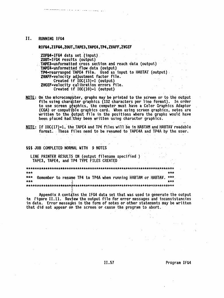
tiQIE.:
II. RUNNING IfG4
RlfQ4.ZIF&4.ZOUT.TAPE3.TAPE4.TP4.ZVAff.ZVCEf
ZIfG4=IFG4 data set nnput)ZOUT=IFG4 results (output)TAPE3=unformatted.cro$s section and reach data (output)TAPE4=unformatted flow data (Qutput)TP4=rearranged TAPE4 file. Used as Input to HABTAT (output)ZVAFF=velocity adjustment factor file.
Created if IOC(13)=1 (output)ZVCEF=veloclty calibration errors file.
Created if 10C(10)=1 (output)
On the microcomJi!lter, graphs may be printed to the screen or to the outputfile using char~~ter graphics (l3Z. characters per line format) •. I.norderto use screen gtaphlcs, the computer must have a Color Graphics Adaptor(CGA) or compatt.lble graphics card. When using screen graphics, notes arewritten to the 9utput file in the positions where the graphs would havebeen placed hadithey been written using character graphics.
tillIE: tfIOC(7)=l, th~ TAPE4and TP4 files will be in HABTAM and HABTAV readableformat. These files need to be renamed to TAPE4A and TP4A by the user.
$$$ JOB COMPLETED NORMAL WITH 9 NOTES
lINE PRINTER RESULTS ON (output filename specified )TAPE3, TAPE4, and TP4 TYPE FILES CREATED
******************************************************* ********~******
*** ****** Remember to renawe TP4 to TP4A when running HABTAM or HABTAV. ****** .:\, ***'[I*********************t************************************************
ijAppendix Acont~ins the IFG4 data set that was used to generate the output
in Figure 11.11. Rev~ew the output file for error messages and inconsistanciesin data. Error messages in the form of notes or other statements may be writtenthat did not appear on the screen or cause the program to abort.
11.57 Program IFG4
The ZVAFF file created by setting IOC(13)=1 Is shown in figure 11.12. The14VAF program can be run to plot or analyze and plot the Velocity Adjustmentfactors (VAF's). Figure 11.13.
By looking at the ZVAff file and the plot, It appears that cross section0.0 needs additional work as the velocity adjustment ,factor~ are in a reversepattern from what they should be. This indicates that IFG4 is underpredlctlngwater surface elevations at the low flows and overpredicting them at the highflows. Cross section 0.0 is basicaly triangular with numerous Irregularities.The three measured points were taken at flows where the water was confined tothe thalweg. As a result, the rating curve for this section Is too steep todescribe the stage-discharge relationship at flows above the high calibrationflow.
Recommend running MANSQ and using the predicted water surface elevationsto see if better results can be obtained. Refer to MANSQ program documentationfor results.
11.58 Program IfG4

SECTIONS OF SAMPLE OUTPUT HAVE BEEN DELETED HERE FOR BREVITY.
ANALYSIS FOR CROSS SECTION 0.00
CALIBRATION OF STAGE - DISCHARGE RELATIONSHIP FOR GIVEN DISCHARGES
DISCHARGE21.800IZ.6007.900
STAGE97.86097.78091.650
PLOTTING STAGE0.6600.5800.450
STAGE OF ZERO FLOW IS 91.20
STAGE - DISCHARGE RELATIONSHIP
LOO - LOG FUNCTION
Q• 0.621£+02 '(STAOE - 97.20 J" 2.623
MEASURED21.80012.6007.900
PREDICTEO20.69013.S177.651
RATIO1.0440.9281.033
MEAN ERROR 5.03VARIANCE 5.84
STD. OEV. 2.42SAMPLE SIZE 3.
Figure 11.11. Sample output from the IFG4 program.
1[.59 Program IFG4
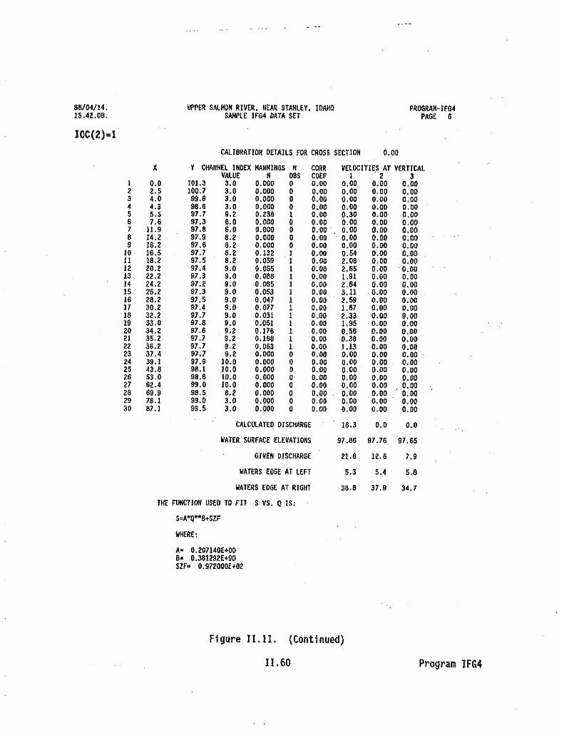
88/04/14. UPPER SALMON RIVER. NEAR STANLEY. IDAHO PROGRAH-I FG415.42.08. SAMPLE IFG4 DATA SET PAGE 6
10C(2)=1
CALI8RATION OETAILS FOR CROSS SECTION 0.00
X Y CHANHEL INDEX HANNINGS N CORR VELOCITIES AT VERTICALVALUE N 08S COEF I 2 3
I 0.0 101.3 3.0 0.000 0 0.00 0.00 0.00 0.002 2.~ 100.7 3.0 0.000 0 0.00 0.00 0.00 0.003 4.0 99.8 3.0 0.000 0 0.00 0.00 0.00 0.004 4.3 98.6 3.0 0.000 0 0.00 0.00 0.00 0.00S 5.5 97.1 9.2 0.238 I 0.00 0.30 0.00 0.006 7.6 91.3 6.0 0.000 0 0.00 0.00 0.00 0.007 11.9 91.6 6.0 0.000 0 0.00 0.00 0.00 0.008 14.2 97.9 8.2 0.000 0 0.00 0.00 0.00 0:009 16.2 97.6 8.2 0.000 a 0.00 0.00 0.00 0.00
10 16.5 97.1 8.2 0.132 I 0.00 0.54 0.00 0.00II 18.2 97.5 8.2 0.059 1 0.00 2.08 0.00 0.0012 20.2 97.4 9.0 0.055 I 0.00 2.65 0.00 . 0.0013 22.2 97.3 9.0 0.086 I 0.00 1.91 0.00 0.0014 24.2 97.2 9.0 0.065 I 0.00 2.84 0.00 0.0015 26.2 97.3 9.0 0.053 1 0.00 3.11 0.00 0.0016 28.2 97.5 9.0 0.047 I 0.00 2.59 0.00 0.0017 30.2 97.4 9.0 0.071 I 0.00 1.87 0.00 0.0018 32.2 97.7 9.0 0.031 I 0.00 2.33 0.00 0.0019 33.0 97.8 9.0 0.051 I 0.00 1.95 0.00 0.0020 34.2 97.6 9.2 0.176 I 0.00 0.56 0.00 0.0021 35.2 97.7 9.2 0.188 1 0.00 0.38 0.00 0.0022 36.2 97.1 9.2 0.063 I 0.00 J.13 0.00 0.0023 37.4 97.1 9.2 0.000 0 0.00 0.00 0.00 0.0024 39.1 97.9 10.0 0.000 0 0.00 0.00 0.00 0.0025 43.8 98.1 10.0 0.000 0 0.00 0.00 0.00 0.0026 53.0 98.6 10.0 0.000 0 0.00 0.00 0.00 0.0027 62.4 99.0 10.0 0.000 0 0.00 0.00 0.00 0.0028 69.9 98.5 8.2 0.000 0 0.00 0.00 0.00 0.0029 78.1 99.0 3.0 0.000 0 0.00 0.00 0.00 . 0.0030 87.1 99.5 3.0 0.000 0 0.00 0.00 0.00 0.00
CALCULATED OISCHARGE 18.3 0.0 0.0
WATER SURfACE ELEVATIONS 97.86 97.76 97.65
GIVeN DISCHARGE 21.8 12.6 1.9
WATERS EDGE AT LefT 5.3 5.4 5.8
WATERS EDGE AT RIGHT 38.8 37.9 34.7
THE FUNCTION USeD TO FIT S VS. Q IS;
S-A*Q**8*SlF
WIlERE;
A- 0.207140E+008= 0.381292E+005zr- O. 972000E+02
Figure 11.11. (Continued)
11.60 Program IFG.4

88/04/14.15.42.08.
UPPER SALMON RIVER. NEAR STANLEY. IDAHOSAMPLE IFG4 DATA SET.
PROGRAM-IFG4PAGE 7
NOTE I WHILE PROCESSING CROSS SECTION 0.00 AN N VALUE WAS NEEDED, BUT NOT SUPPLIEDFOR SEGMENT 6 0.13200 WAS USED
NOTE 2 WHILE PROCESSING CROSS SECTION 0.00 AN N VALUE WAS NEEDED, BUT NOT SUPPLIEDFOR SEGMENT 23 0.06308 WAS USED
NOTE 3 WHILE PROCESSING CROSS SECTION 0.00 AN N VALUE WAS NEEDED, BUT NOT SUPPLIEDFOR SEGMENT 24 0.0630B WAS USED
NOTE 4 WHILE PROCESSING CROSS SECTION 0.00 AN N VALUE WAS NEEDED, BUT NOT SUPPLIEDFOR SEGMENT 25 0.06308 WAS USED
NOTE 5 WHILE PROCESSING CROSS SECTION 0.00 AN N VALUE WAS NEEDED. BUT NOT SUPPLIEDFOR SEGMENT 28 0.06308 WAS USED
SECTIONS OF SAMPLE OUTPUT HAVE BEEN DELETED HERE FOR BREVITY.
88/04/14.15.42.08.
UPPER SALMON RIVER, NEAR STANLEY, IDAHOSAMPLE IFG4 DATA SET
PROGRAM-IFG4PAGE 13
NOTE 6 WHILE PROCESSING CROSS SECTION 14.30 AN N VALUE WAS NEEDED, BUT .NOT SUPPLIEDFOR SEGMENT 10 0.13173 WAS USED
NOTE 7 WHilE PROCESSING CROSS SECTION 14.30 AN N VAlUE WAS NEEDED. BUT NOT SUPPLIEDFOR SEGMENT 26 0.04081 WAS USED
NOTE 8 WHILE PROCESSING CROSS SECTION 14.30 AN N VALUE WAS NEEDED, BUT NOT SUPPLIEDFOR SEGMENT 8 0.13173 WAS USED
NOTE 9 WHILE PROCESSING CROSS SECTiON 14.30 AN N .VAIUE WAS NEEDED, BUT NOT SUPPLIEDFOR SEGMENT 29 0.04081 WAS USED
IOC(19)-lSUMMARY OF. CALIBRATION FLOWS (CFS)
CROSSSECTION
0.0014.30
MEANSSTO DEV
COEF OF VARIATION
$$$ JOB COMPLETED NORMALLY WITM 9 NOTES
I21.8021.80
21.800.00
0.000
212.6012.60
12.600.00
0.000
37.907,90
7.900.00
0.000
Figure II.ll. (Concluded)
II. 61 Program IFG4
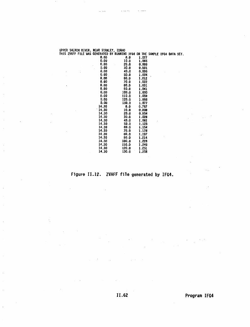
UPPER SALMON RIVER, NEAR STANLEY, IDAHOTHIS lVAFF FILE WAS GENERATED 6Y RUNNING IFG4 ON THE SAHPLE IFG4 DATA SET.
0.00 6.0 1.0770.00 10.0 1.0650.00 20.0 0.9990.00 30.0 0.9910.00 40.0 0.9960.00 50.0 1.0040.00 60.0 1.0120.00 70.0 1.0220.00 60.0 1.0310.00 90.0 1.0410.00 100.0 1.0500.00 110.0 1.0590.00 120.0 1.0680.00 130.0 1.077
14.30 8.0 0.767. 14.30 10.0 0.606
14.30 20.0 0.95414.30 30.0 1.02814.30 40.0 1.08114.30 50.0 1.12314.30 60.0 1.15414.30 70.0 1.17814.30 80.0 1.19714.30 90.0 1.21414.30 100.0 1.22814.30 110.0 1.24014.30 120.0 1.25114.30 130.0 1.256
Figure 11.12. ZVAFF file generated by IFG4.
11.62 Program IFG4

/1SIf1Yl'S. ~ &IlKiI RlIB. lINt IIfNlEf, IIl\lD_, 14VN'
QI1.55.07. WAle IFGI MTA SET IWE' I
I.3illI .. I I I I I I . I I II.. I , , I , I , I I/... , , , I , I , , I/... I/.l.lI!IXl ..... B •...1/.
I/. B I/.I/. B I/... B I/.
• I I/.I,lID) ..... B ....1/.
• III/. B I/... .... B It
1.140) ..... ",,11It B II• IIII III/. 1/
I.IB» ....1. I A •.. ·11II A A 1/I/. A II
II\F II A A III/. I A II
, .0i!lJ0 ".... A ",,1/... A A ..I/. A A A IIII II• •0._ ".... B .....II •II IIII II• II
0.9Iml ..... ...,... II.. I/.I/. IIIt II
O,llIOOO ..... ,,,,11
• ..I/. II• B III/. It
0.70000 ..... ..··11• B It.. 1 I I 1 1 1 1 1 1 II.. 1 , I 1 1 1 1 , 1 II1# I I I 1 I I 1 1 1 It
0.7<0000.00XQ!·01 I,O,OCO OO.OCO 131.00 160.00 200,00
2O.0c0 6O.0c0 100.00 11,0.00 110,00
DI_
VElClCIlY 1NJSlIflIf _ 'IS. DlSClWlGE fllR srATlalS 0,00 TlRJ 14,31)
Figure 11.13. Plot of ZVAFF file generated by IFG4.
11.63 Program IFG4
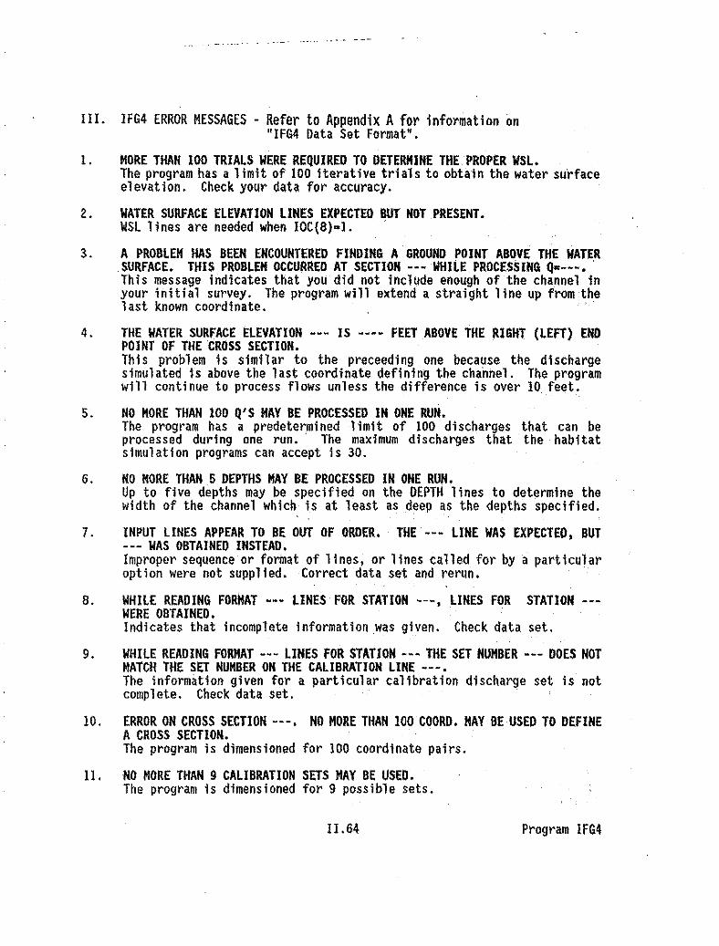
III. IFG4 ERROR MESSAGES - Refer to Appendix Afor information on"IFG4 Data Set Format".
1. MORE THAN 100 TRIALS WERE REQUIRED TO DETERMINE THE PROPER WSL.The program has a limit of 100 Iterative trials to obtain the water surfaceelevation. Check your data for accuracy.
2. WATER SURFACE ELEVATION LINES EXPECTED BUT NOT PRESENT.WSL lines are needed when IOC{8)Ql.
3. A PROBLEM HAS BEEN ENCOUNTERED FINDING A GROUND POINT ABOVE THE WATERSURFACE. THIS PROBLEM OCCURRED AT SECTION --- WHILE PROCESSING Qw •This message indicates that you did not include enough of the channel inyour initial survey. The program will extend a straight line up from thelast known coordinate. '
4. THE WATER SURFACE ELEVATION --- IS ---- FEET ABOVE THE RIGHT (LEFT) ENDPOINT OF THE 'CROSS SECTION.This problem is similar to the preceeding one because the dischargesimulated is above the last coordinate defining the channel. The programwill continue to process flows unless the difference is over 10 feet.
S. NO MORE THAN 100 Q'S MAY BE PROCESSED IN ONE RUN.The program has a predetermined limit of 100 discharges that can beprocessed during one run.' The maximum discharges that the habitatsimulation programs can accept is 30.
6. NO MORE THAN 5 DEPTHS MAY BE PROCESSED IN ONE RUN.Up to five depths may be specified on the DEPTH lines to determine thewidth of the channel which is at least as deep as the depths specified.
7. INPUT LINES APPEAR TO BE OUT OF ORDER. THE --- LINE WAS EXPECTED, BUT--- WAS OBTAINED INSTEAD.Improper sequence or format of lines, or lines called for by a particularoption were not supplied. Correct data set and rerun.
8. WHILE READING FORMAT --- LINES FOR STATION _OM, LINES FOR STATION --WERE OBTAINED.Indicates that incomplete information ,was given. Check data set.
9. WHILE READING FORMAT --- LINES FOR STATION --- THE SET NUMBER --- DOES NOTMATCH THE SET NUMBER ON THE CALIBRATION LINE '--.The information given for a particular calibration discharge set is notcomplete. Check data set. .
10. ERROR ON CROSS SECTION ---. NO MDRE THAN 100 COORD. MAY BE USED TO DEFINEA CROSS SECTION.The program is dimensioned for 100 coordinate pairs.
11. NO MORE THAN 9 CALIBRATION SETS MAY BE USED.The program is dimensioned for 9 possible sets.
11.64 Program IFG4

12. OPTION FOR STAGE-Q RELATIONSHIP SELECTED WITHOUT Q'S BEiNG PROVIDED.You must supply stage data if IOC(8)-Z. The program will abort.
13. HAViNG TROUBLE FINDING A NON-ZERO CALIBRATION VELOCITY WHEN COMPUTiNGMANNiNG'S N. WHiLE PROCESSING SECTiON··· POINT ••••The program will abort. This indicates that standjng water is beioganalYled.
..14. THERE IS A PROBLEM ON CROSS SECTION ••- \lITH THE VELOCITIES AND THE
COORDINATES AT VERTICAL ...• AVELOCITY HAS BEEN GIVEN (..•) BUT THE DEPTH(_._) BASED ON THE WSL (_OM) IS NEGATIVE.Program may not abort; message will be in output file indicating thatthere may be an error in data; or, the water surface elevation based ona flat surface is different from the actual water surface elevation at thevertical.
15. FOR THE CROSS SECTION --- THERE ARE -- CELLS IIITH THE SLOPE IN THE VELOCITYVS. Q RELATIONSHIP GREATER THAN 3. SUGGEST USING ANOTHER APPROACH TOHYDRAULIC SIMULATION.This will cause run to abort. To override the abort, set IOC(2l)-l.
16. ZERO DISCHARGE COMPUTED AT CROSS SECTION --- AND SET _OM.Program run continues. Message is in output file.
17. WHEN IOC(8)-2AND THE VELOCITIES ARE NOT SUPPLIED, THE CALCULATED Q.MUSTBE ON THE CAL LINE.This will cause run to abort.
18. THE WATER SURFACE ELEVATION --- FOR Q --- IS BELOII THE LOIIEST POiNT ONTHIS CROSS SECTION ---, THIS PROBLEM is BEING CORRECTED BY SETTiNG THEWSL TO 0.1 FEET ABOVE THE LOW POINT ON THE XSEC.Program run continues; message is in output file.
19. FOR CROSS SECTION --- AND CALIBRATION SET .-- FOUND A ZERO FLOII WHEN ANON-ZERO FlOII liAS NEEDED FOR LEFT AND RIGHT STAGE ANALYSIS.IOC(IS)=1 and the calibration flow for this set is equal to lero. SetlOC(IS)=O as this option has not yet been implemented in any of theprograms in PHABSIM other than IFG4.
20. ZERO OR NEGATIVE DISCHARGE NOT ALLOWED. DISCHARGE----.Program will abort.
21. ENDJ LlNE NOT FOUND. . .The last line of an IFG4 data set must contain "ENOJ" in columns 1·4.
22. IOC(8) NOT EQUAL TO 1 AND TOTAL NUMBER OF CAL IBRAT IOH SETS-I. UNABLE TOCREATE A RATING CURVE IIITH ONLY ONE POINT.Program will abort.
23. OPTION TO READ CALCULATED FLOW SELECTED. FLOW READ liAS ZERO. RUNTERMINATING.IOC(5) was set to "I" and the calculated flolf was zero.
11.65 Program IFG4

24. PROBLEH AT CELL •• SLOPE IN VELOCITY REGRESSION IS IRRATIONAL. NOT AGOODSIMULATION OF VELOCITIES, USE ANOTHER APPROACH. ALL VELOCITIES AT CELL._. ARE SET TO 0.0. SLOPE IS -_.•Recommend running a different hydraulic simulation program to determinewater surface elevations; add these WSL's to the IFG4 data set, and runIFG4 again to see if .better results are obtained.
25. WHEN NO VELOCITY IS SUPPLIED AND CALCULATED Q IS NOT GIVEN, IOC{S) MUSTBE 1.Program will abort.
26. DEPENDENT VARIABLE IS LESS THAN OR EQUAL TO ZERO. NOW SET EQUAL TO 0.01,REVIEW YOUR DATA.Regression analysis for theshge-discharge relationship cannot be doneusing zero values for discharge. A ,l;ero discharge was found and made0.• 01. Most likely there is a data problem.
27. BAD DATA·CHE~ YOUR DATA, LOG OF COEFFICIENT ASET EQUAL TO .299.0.for some reason an unrealistic stage.discharge relationship was determined.The relationship was modified so that the program would not abort. Adataproblem exis~s and. should be fixed.· .
28. WITH LESS THAH :3 SETS OF VELOCITY MEASUREMENTS IOC(14) HUST BE SET TO ZERO.Program will abort.
29. THE WIDTH IS A NEGATIVE NUMBER •• (XL,XR-·-) IN SUBROUTINE-SLICE WHILEPROCESSING SECTION .. FOR Q-_.-.Suggests error in coordinate data.
30. STAGE· STAGE OF ZERO FLOW IS LESS THAH OR EQUAL TO ZERO FOR SET "Probably an error in recording water surface elevations. At a certainflow (set #), the stage of zero flow is greater thah the water surfaceelevation.
31. WHILE PROCESSING CROSS SECTION --- AN NVALUE WAS NEEDED, BUT NOT SUPPLIEDFOR SEGMENT .--, _._.-.- WAS USEDThe wf11 appear as a note in the IFG4 output fne~ This message occursWhen a vertical was dry for the calibration data set and a N value wasnot assigned. In the simulation proce~s the program searches adjacentcells until a Nvalue is found; this value of N is used. If no Nvaluesare found, a value of 0.06 is used. The user should review the resultsto see if the N's actually used are reasonable.
11.66 Program IFG4
IFG4IN Program
I. INTRODUCTION·
The IFG4IN program is available on the microcomputer to enter and/or editan IFG4 data set. It also performs several checks on the data as it is beingentered. The TREVI4, RCKI4, or REVI4 batch/procedure files could also be runto check the complete data set prior to running the IFG4 program.
The IFG4IN program has the following limitations and assumptions:
ACCURACY
- The option which calculates the discharge given X,V coordinates and the cellvelocities is based on a method that is more elaborate than. is typicaly usedwhen one does this with a hand calculator. Specifically, the cell is definedas being vertically centered. The width of each cell is calculated as being fromthe half-way points to the neighboring verticals. The depth .is calculated asbeing the average of that vertical and each of the neighboring verticals. Theseaverage widths and depths are then multiplied times the given vertical's velocityand summed across the channel for the total flow. (Q). Results should becomparable with other popUlar methods under most circumstances, but do not expectexact cOljlparison. If there is a large difference, you have probably donesomething wrong, and that is what this part of the program is for.
- The screen graphiCS resolution may not be capable of displaying all pointson a graph.
KNOWN DEfICIENCIES
- The program does not check for eVery possible combination of IOC parameterswhich may cause mathematical "blowup" in the IFG4 program.
- Once a line has been added, it cannot be deleted. An external editor mustbe used to delete the line.
- CAL lines must be numbered sequentially starting with 1. The IFM programwill accept almost any sequence of numbers such as 2, 4,6.
- The program does not contain the ability to incorporate the instrument heightinto bed elevation data.
Additional cross sections cannot be added to an existing data set. Anexternal editor may be used to merge cross section data.
ASSUMPTIONS
- Assumes that the input files are "legally" formatted (syntactically correct)when read into memory. At least the two title lines, IOC line, and one crosssection (coordinates plus NS lines) must be present. If a formatting error ispresent, the user will be informed of a probable error, but the program may
11.67 Program IFG4IN

ignore the error and continue on. If this should occur, "Ctrl-Break" out of t.heprogram and use an external editor to correct the problem.
Each parameter has built-in upper and lower bounds to attempt to preventoutlandish user input. errors. An external editor can be used to change the datavalues if needed.
- Assumes that stationing is used as cross section Identification numbering.
- Will not allow VEL lines to be added unless there is a corresponding CALline.
- Assumes that QARU flows should be entered from low to high.
II. RUNNING IFG41N
RIFG4IN
User will be prompted for filename. If an eXisting data set is beingedited, the unedited version of the file will be saved with a .BAKextension.
This program is not available on the CDC.
The program is organized in a hierarachical menu system. By folloWing themenus, one may step forward and backward through the system as the need dictates.
An introductory screen will appear showing the version of the program andthen the following "main" menu will appear.
IfG4 PATA ENTRY AND EDITING
O. Exit this program
1. Get an existing IFG4 data set from disk2. Enter a new data set for IfG43. Select New Transect Data4. Edit IFG4 data set5. Scrutinize an IfG4·data set6. List IFG4 data set7. Set program defaults (not implemented yet)
You must first either ENTER or GET a data set. When "getting" an eXistingdata set, the filename must have ". IN4" as the MS/POS extension; the versionbefore editing will be saved with a ".BAK" extension. Data sets befng "entered"are automatically assigned the ".IN4" extension.
One cross section (transect) is worked on at a time when entering orediting a data set..
11.68 Program IFG4IN

-_ ... _- .... .. . . . . .-. - _..... -
At various times, error or warning messages may be printed to the screen.These will be preceeded by a beeping sound to alert the user to a probable error.
Almost all prompts are accompanied by a "default" answer which is activatedby pressing the. EtHER (or RETURN) key. The defaults for some prompts, usuallyyes or no questions, may be displayed in brackets []. The defaults for mostother prOll1pts will be shown on the screen.
EDITING KEYS
- The ENTER key stores new values.- The ESC key gets you out of most editing areas.- New data points may be inserted by pressing the INS key .or deleted
by pressing the DEL key. .• The up and down arrows are operable; the left and right arrows are
not. The up and down arrows will not store a value, thus, the onlyway to leave a field blank is to press the down arrow "over" thefield. It is unwise to leave blank fields on any lines exceptVEL's and Manning'S II.
- Two data entry/editing areas use the TAa key to get from one datatyee to another and back again. These are (X and V) and (II and S).
- A Ctrl-Break" will exit the program completely. liD changes willbe stored.
Refer to Appendix A for a sample IFG4 data set.
11.69 Program IFG41N

lPTTHWE Program
I. INTRODUCTION
The lPTTHWE program plots the Thalweg values and water surface elevationsfor given discharges from a TAPE3 and TAPE4 generated by the hydraulic simulationprograms. A graph of the coordinate points for each cross section is alsogenerated along with a table containing the water surface elevations in relationto given distances, Thalwegs, and discharges.
II. RUNNING lPTTHWE
RLPTHWE.LPTOUT.TAPE3.TAPE4
LPTOUT~lPTTHWE results (output)TAPE3=unformatted cross section and reach data (input)TAPE4=unformatted flow data (input)
~: On the microcomputer. graphs may be printed to the screen or to the outputfile using character graphics (132 characters per line format). In orderto use screen graphics, the computer must have a Color Graphics Adaptor(CGA) or compatible graphics card. When using screen graphics, notes arewritten to the output file in the positions where the graphs would havebeen placed had they been written using character graphics.
Figure 11.14 contains sample output from the lPTTHWE program.
III. ERROR MESSAGES
STATION ON FLOW FILE --- NOT FOUND ON CIS FILE
The TAPE3 and TAPE4 have different Cross Section ID Numbers in them. Theywere probably created using different data sets or CHSTA4 was run on theTAPE4 to change cross section ro numbering; the TAPE3 cross sectionnumbering was not changed.
n.70 Program lPTTHWE

8Il.iW01. ~ _ Rl\lill. fI1Jjl $TNUY. IIWI:l_ • I.P11lIoE
10.41.36. lIW'tE 1fG> MTA $Ef_.
I
112.1ll1/ 1 1 1 1 1 I 1 1 1 ,, 1 1 1 1 1 1 I 1 1 ,, 1 I 1 I 1 1 1 1 1 1/1/ 1/
101.50 •••• ····f, ,• ,, •, ,
101.1ll •... ....,1/ ,1/ /I1/ • /I1/ ,
IIll.5O ,.... ....,, /I, 1/, ,, /I1OO.1ll '•... ····f, ,, • •ELiVATllJl 1/ 1/, ,99.500 I/o ••• .•..,, /I
II ,1/ ,, ,
99.em •••• • ....,1/ ,, ,, /I1/ • • ,
Sl8.51ll •... • ..;.,, ,1/ 1/1/ ,, • ,
Sl8.em 1/.... ....,, • • 1/, 1/1/ • • • ... ,1/ • • .. ,
97.500 ..... • • ..••1/, • • ,, '1 1 • ., 1 1 1 1 ,1/ 1 , • 1 , , 1 1 f1/ 1 1 1 I I I 1 ,
97.em0'_'01 IS.em 36.em "'.em 7Z.em 9O.em
9.00l0 21.em 4S.em /is.em 1I1.em
01$TNa
ao;s I£CTllJI 0.00 AT lOTH. IlfAtlI talGIlI a- 0.1ll
Figure 11.14. Sample output from the lPTTHWE program.
11.71 Program lPTTHWE

88{05{01.10.41.36.
UPPER SALMON RIVER, NEAR STANLEY, IDAHOSAMPLE IFG4 DATA SET
PROD· LPTTHIIEPAGE - 3
DISTANCE THALIlEG 130.00 120.00 110.00 100.00 90.00 80.00 70.00
0.0 97.20 98.53 98.49 98.44 98.40 96.35 98.30 98.2514.2 97.60 98.63 96.80 98.76 98.72 96.66 96.63 96.58
DISTANCE TNALIlEG 50.00 50.00 40.00 30.00 20.00 10.00 8.00
0.0 97.20 98.19 98.12 98.05 97.95 97.85 97.70 97.6814.2 97.60 98.53 96.47 96.40 96.32 98.22 98.08 98.04
ONLY THE DATA GENERATED FOR THE FIRST CROSS SECTION AND ONE FLOW HAVE BEENINCLUDED IN THIS SAMPLE OUTPUT.
Figure 11.14. (Continued)
11.72 Program lPTTHWE
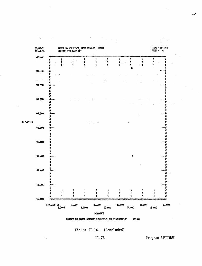
ll\IO$/Ol. lI'I'ER SAUDI RIVER, lEN! STAlILEY, IMOO PIm • IPTIIWilQ.41.!6. SIll'l.E Ii'll> DATA SEI PNiIl • 4
99.000 • 1 1 , 1 1 1 1 1 •, 1 1 1 1 1 1 1 1 ,, 1 1 1 1 1 1 1 1 ,, B ,16.000 ff- ••• ····It
It It, It, ,, ,16.6QO ff- ••• ....,, It
B #, ,It #
16.400 ,.... ····It
• ,, ItIt ItIt ,
16.<00 It···· ....,It #, ,
ElEVATtCll It ItIt ,
16.000 ,.... ••••#, /I• ItIt ,, ,
'17.000 ,.... ....,It •It ,It ,/I #
V7.(H) It···· ....,It It, It, #It #
'17.400 11- ••• ••••#It #It #It ,• It
'17.<00 A' ••• ····It/I /I, 1 1 1 1 1 1 1 1 ,, 1 1 1 1 1 1 1 1 /I• 1 1 1 1 1 1 1 1 #
V7.rI1J
O.lJlXm;·Ol 4.00lQ 8.croJ 12.rI1J 16.rI1J 2O.rI1J2.00lQ 6.00lQ 10.rI1J 14.rI1J 18.rI1J
OlsrNlE
TIW.lI!ll AN1 ~1S! SUlFACE ElEVATlCllS A:R DISCIWlGE Of' 130.00
Figure II.14. (Concluded)
11.73 Program LPTTHWE

MAKIVl Program
I. INTRODUCTION
The MAKIVL program reads an IFG4 data set and writes anew IFG4 data setwith one or less velocity sets.
II. RUNNING MAKIVL
RMAKIVL;ZIFG4.ZIFG4N
ZIFG4=IFG4 data set (input)ZIFG4N=new IFG4 data set with one or less velocity sets(output)
User will be prompted to
ENTER SET NUMBER FOR VELOCITY.SET TO BE RETAINED:
The velocity set specified will be kept: all other velocity sets will beblank. If a '0' or a number that is not a set in the data set isspecified, all velocity sets will be blank.
n.74 PrograrnMAKIVL
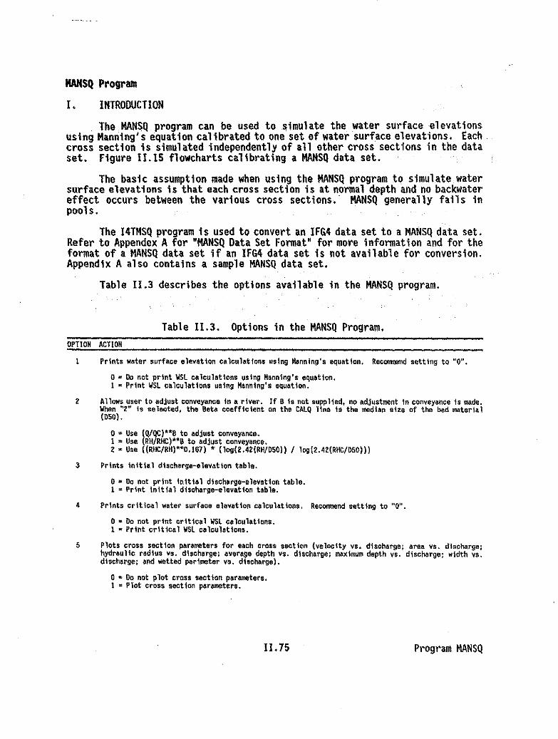
HAHSQ Pl'ogrlll1l
I. INTRODUCTION
TheMANSQ program can be used to simulate the water surface elevationsusing Manning's equation calibrated to one set of water surface elevations. Eachcross section is simulated independently of all other cross sections in the dataset. Figure 11.15 flowcharts calibrating a MANSQ data set.
The basic assumption made when using the HANSQ program to simulate watersurface elevations is that each cross section is at normal depth and no backwatereffect occurs between the various cross sections.· MANSQ generally fails inpools.
The I4TMSQ program is used to convert an IFG4 data set to a MANSQ data set.Refer to Appendex Afor "MANSQ Data Set Format" for more information and for theformat of a MANSQ data set if an IFG4 data Set is not available for .conversion.AppendiX A also contains a sample HANSQ data set.
Table 11.3 describes the options available in the HANSQ program.
Table 11.3. Options in the MANSQ Program.OPTION ACTION
1 Prints w~ter surface elevation ealcul~tfQns using Manning's equation. RecQIl'Illend setting to "0".
o • 00 not print VSL c41culotlons using Manning's equation.1 ~ Print WSl calculattons using Hanning's equ~tion.
2 Allows user to adjust conveyance in a rtVEtf. If B ts not supplied, no adjustment in conveyance is made.When "2" i$ seloot-ed. the Beta cQefftc'ent on the CAlQ Hne is the It'ledtall size of the bed material(OSO).
o =Use !Q/QC)"8 to adjust conveyance.1 =Use RH/RHC)"S to adjust conveyonce.z· Use «RHC/RH)··0.167) • (log(2.42(RH/DSO» I log(2.42(RHC/DSO»)
3 Prints initial dischltrge~ele~ationtable.
o• 00 not print Inlt141 dlschorgo-elevot10n table.1 = Print tnitfal disonarge-elevatfon table.
4 Prints critical water surface elevetion calculations.. Recom:nend setting to "0".
o • Do not print critical WSl calculations.1 • Print orlt1001 VSl calculotlons.
5 Plots cross section pftrameters for each cross Duction (velocity vs. disohArge~ Area vs. discharge;hydraulic radius vs. di,eharge: ~verage depth vs. discharge; maximum depth V$. discharge; width va.discharge; ond wetted Perimeter vs. dlschargo).
o & 00 not plot cross section parameters.1 = Plot cross section par4meters.
11.75 Program HANSQ

Table II.3 (Concluded)OPTIO~ ACTIO~
6 Allows the hydraulic radius for a cell to be weighted by the area in a c.ll which results In an .reaweighted hydroulic radiu.. Recommend ••ttlng to one "1".
o= Use normal hydraulic r.dlus (R=AREA/(WfTTEO PERIMETERll1 • Ose area we\ghted hydraulic radtus.
1 Plots the Stage~ Relat'onsh\p detennined using Manning's equation and the critical water surfaceelevation calcul~tio"s.
o • log-log plot.I • Arlthmatic .nd log-log plots.2 • No plots.
a Generates a plot of the cross section coordinate points.
o w Do not plot cross sections.1 z Plot CTDSS sections.
9 Determines select10n of velocity equation.
o ~ Use Hann'ng's equation.1 = Use CheZY'S equation.
10 Prov1des for modifle.tlon of the hydraulic radius.
o = Do not modify hydraulto radtvs.1 = Hydraulic radius is reduced by the hydraulic radius
at the stage of zero flow.
11 Writes ve1oc1ties to TAPE4 using the criteria below. The nonmal ~pproach is to average the velocityat the verticals defining the tight and left side of a cell to determine that cell~s velocity.
o ~ Write mean velocity for the whole cross section.I • Write nonnal cell velcelti•• (HABTAT format).2 = Write velocities at wet vertfcals (HABTAV and HA8TAM
format).3 = Write velceltie. ot 011 verticl.s (re.ulting TAPE4
is not for use with PHABSIM programs).
12-19 Reserved for futute options.
20 Multlpli.s the eros. section width by a constant.
0 0 Multlpl1er = 1 (i .•.• multiplier" 10**IOC(20) valuel·1 • Multiplier ~ x given * lO*kl (used on large rivers)
(I .•.• multiplIer' IO**IOC(20) v.lue).2 • Multiplier ~ x given ~ lO**Z (used on large rivers)
(I.e .• multIplier' 10**IOC(201 volu.).3 = Multiplier • ~ given * 10··-1 (used on small rivers)
.(i.e.• multiplier' IO'*(2-IOC(201 v.lue)l.4 - Multipler = x given ~ 10**-2 (used on small rivers)
(I.e.• multiplier' IO'*(2-!OC(20) value)).
11.76 Program MANSQ

CALIBRATING A MANSQ DATA SET
~
~........... MANSO
repeat untilWSL·scal1brated 0
MODQARO or editor(place simulation flowson QARD lines inMANSO data set}
MANSO
'"" -
.&...!§i
~VI.0
Figure 11.15.- Calibrating a MANSQ Oata Set.

NOTE:
II. RUNNING MANSQ
RHANSQ.ZMANSQ.ZOUT,TAPE3,TAPE4
ZHANSQ=MANSQ data set (input)ZOUT=MANSQ results (output)TAPE3=unformatted cross section and reach data (output)TAPE4=unformatted flow data (output)
On the microcomputer, graphs maybe printed to the screen or to the outputfile using character graphics (132 characters per line format). In orderto use screen graphics. the computer must have a Color Graphics Adaptor(CGA) or compatible graphics card. When using screen graphics, notes arewritten to the output file in the positions where the graphs would havebeen placed had they been written using character graphics.
Appendix Acontains the MANSQ data set that was used to generate the outputin Figure 11.16. Review the output file for error messages and inconsistanciesin data. Error messages in the form of notes or other statements may be writtenthat did not appear on the screen or cause the program to abort. .
When IFG4 was run on the sample IFG4 data set, it was determined that the. rating curve for the first cross section was too steep to describe the
stage-discharge relationship at flows above the high calibration flow.Therefore, it was recommended that MANSQ be run to determi ne water surfaceelevations as It incorporates the expansion of cross sectional area as flowsIncrease and does a better job of predicting the correct stages.
In this case, MANSQ significantly improves the results for the first crosssection, but does not improve the results of the second cross sectionappreciably. The second cross section is a parabolic section, so the slope ofthe rating curve will be nearly constant from low to high flow.
III. ERROR MESSAGES
Most of the errors in MANSQ are due to data set format errors. Refer toAppendix Afor "MANSQ Data Set Format". Also refer to error message section hithe IFG4 program documentation, as several of the errors messages are the same.
I . ERROR AT SECTION ---, CALQ EXPECTED BUT NOT FOUND.Check data set. Make sure that there is a CAlQ(not CAL} line for eachcross section.
2. NO HORE THAN ONE CALIBRATION SET MAY BE USED lIHlLE PROCESSING CROSS SECTION-- ....The program Is dimensioned for one CAlQ line per cross section.
3. USING ANEGATIVE BETA COEFFICIENT. HOST OFTEN BETA IS POSITIVE IN HAHSQ.This is a warning; the program will not abort. At one time the betacoefficient had to be entered as a negative value. This is no longer thecase.
11.78 Program MANSQ

88/06/28. UPPER SALMON RIVER, NEAR STANLEY. IDAHO PROGRAN - MANSQ16.03.15. SAMPLE MANSQ DATA SET-CREATED FROM IFG4 DATA SET USING THE 14TMSQ PROGRAM PAGE - I
WHtN THE FLOW IS SUPER CRITICAL (FROUDE NO. IS GREATER THAN LO) THECRITICAL WATER SURFACE ELEVATION IS WRITtEN ON THE HYDRAULICS PROPERTIESFIlE (TAPE4).
IDC. 0 0 I 0 I I I I 0 0 0 0 0 0 0 0 0 0 0 0o 0 0 000 0 0 000 ODD 0 0 0 0 0 0
ONLY THE OUTPUT FOR CROSS SECTION 0.0 HAS BEEN INCLUDED IN THIS SAMPLE OUTPUT.
CROSS SECTION 10 NUM8ER: 0.00
REACH LENGTH DOWNSTREAM: 0.00 WEIGHT ON SECTION: 0.30STAGE OF ZERO FLOW: 97.20 GIVEN SLOPE, 0.02667000
CF • CFC"((Q/OC)"" 0.10)
COORDINATE DATA PAIRS - THERE ARE 30 POINTS
DISTANCE 0.0 2.5 4.0 4.3 5.5 7.6 11.9 14.2 16.2 18.5ELEVATION 101.3 100.7 99.8 98.6 97.7 97.3 97.6 97.9 97.5 97.7CHANNEL INDEX 3.0 3.0 3.0 3.0 9.2 8.0 6.0 8.2 8.2 8.2
DISTANCE 18.2 20.2 22.2 24.2 26.2 28.2 30.2 32.2 33.0 34.2ELEVATION 97.5 97.4 97.3 97.2 97.3 97.5 97.4 97.7 97.6 97.6CHANNEL INDEX 8.2 9.0 9.0 9.0 9.0 9.0 9.0 9.0 9.0 9.2
DISTANCE 35.2 36.2 37.4 39.1 43.8 53.0 62.4 69.9 78.1 87.1ELEVATION 97.7 97.7 97.7 . 97.9 98.1 98.6 99.0 98.5 M.O 99.5CHANNEL INOEX 9.2 9.2 9.2 10.0 10.0 10.0 10.0 8.2 3.0 3.0
CA1I8RATlON STAGE IS 97.860 CALIBRATION DISCHARGE IS 21.80CROSS SECTIONAL AREA IS 11.32 HYDRAULIC RADIUS IS 0.41
AVERAGE DEPTH IS 0.34 MAXIMUH OEPTH IS 0.66LOW POINT ON CROSS SECTION .15 97.20 STREAM WIDTH IS 32.90
WETTED PERIMETER IS 33.13
WATER TRANSPDRT PARAMETER (1.49"(S"".5)/N) IS 3.52
Figure 11.16. Sample output from the MANSQ program.
II. 79 Program MANSQ

~ lm3l Sill.IOI Rlll:R. _ STANLEY. IMOO _.IW$lMs.1J. srHU _ MTA SIIT·CllfAT1!J) f1Q\ IfGIt MTA SlIT USING TIE 141MSQ_ PAG! • 3
102.00 , 1 .1 1 1 1 I ,mAPl! GEIalATBl \I£N , 1 1 1 1 1 1 ,1(I;(8r-l , 1 1 I 1 1 1 ,, ,
101.so ,.~ .. ....,, ,• ,, ,, ,
101.00 ...... ....,, ,, It
It • II, It11X1.50 if-+ •• ••--#, #
# #It ,# ,
11X1.oo #•••• ....,, ## • .#
ELE\lATJOI # ## #
W.5I» ..... .*H#I.# ## #• •• ,
99.llXl ..... • • ....,# ,, ,# ,It • • #
1ll.5I» ..... • ....,, ,# #, ,, • #
lll.llXl fl. ••• ••••## • • ,• ## • • ..... ,It • • ... ,
97.$00 ,.... • • ....,, • • ,, ·1 1 • '1 1 1 1 1 1 ,• 1 1 • 1 1 1 1 1 1 ,• 1 1 1 1 1 T T 1 ,
'J7.llXlO.\lIXIIl(E·01 18.llXl 36.llXl S4.llXl ?2.llXl llO.llXl
9.0IXIl Z/'.llXl 45.llXl 63.llXl 81.000
OISTN«:E
0lCSS5ECT10I 0.00
Figure 11.16. (Continued)
11.80 Program MANSQ

66/061Z6, UPPER SAL~H RIVER. HEAR STAMLEY, IDA~ PROGRAM - MAHSQ16.03,15. SAMPLE MAHSa DATA SET-CREATED FROM IFG4 DATA SET USIHG THE 14TMSQ PROGRAM PAGE - 4
TABLE GENERATED WHEN10C(3)=1
IHITIAL DISCHARGE ELEVATION TA8LE (a,WSL)-
0.1 97.300 0.5 97.400 1.7 97.500 4.4 97.6009.0 97.700 16,2 97.800 21.8 97.880 28.0 97'.900
38.7 98.000 54.3 98,100 73.0 98.200 94.9 98.300120.0 98.400 148.4 98.500 180,4 98.600 217.1 96.700258.5 98.800 304.8 98,900 356.8 99.000 415.8 99.100480.9 99.200 552.0 99.300 629.1 99.400 112.2 99.500802,1 99.600 898.1 99.700 999.9 99.600 1107.6 99,900
1221.1 100.000 1340.3 100.100 1485.2 100.200 1595,7 100,3001731.9 100.400 1873.6 100.500 2020.9 100.600 2173.7 100,7002332.2 100.800 2496,2 100.900 2665.8 101.000 2840.9 101.1003021.6 101.200 3207.9 101.300
CROSS SECTION 10 HUM6ER' 0.00
DISCHARGE W.S. ELEV. VELOCITY AREA HY RADIUS AVE DEPTH MAX DEPTH WIDTH WP WTP
8.00 97.68 1.36 5.88 0.28 0.23 0.48 25.76 25.91 3.1810,00 97,72 1.47 6.62 0.30 0.23 0,52 29.41 29.57 3,2520.00 97,84 1.88 10.74 0.39 0,33 0.84 32.48 32.70 3.4930.00 97.93 2.17 13.81 0,46 0.40 0,]3 34.71 34.97 3.6340,00 98.01 2.42 16.51 0.52 0.45 0.81 36.59 36.88 3,7450.00 96.08 2.63 18.98 0,58 0.50 0,86 36.23 38.54 3,8260.00 98.13 2.82 21.24 0,62 0.54 0,93 39.50 39.83 3.8970.00 98.19 3.00 23,32 0.66 0.58 0,99 40.52 40.88 3.9580.00 98,23 3.16 25.34 0,70 0.61 1.03 41.49 41.87 4.0190.00 98.28 3.31 27.22 0.74 0,64 1.08 42.38 42.17 4.05
100,00 98,32 3.44 29.04 o.n 0.67 1.12 43.22 43.62 4.10110.00 96.36 3.57 30.81 0.81 0.70 1.16 44.02 44.44 4.14120,00 98,40 3.70 32,48 0.83 0.73 1.20 44.75 45.18 4.17130.00 98,44 3.81 34.16 0.88 0.75 1.24 45.50 45.94 4.21
WSL', VRITTEH TOHYD. PROPERTIES
DISCHARGE HANRIHG CRITICAL FROUDE NUM8ER FILE (TAPE4)
8,00 97,66 97.57 0.50 97.6810,00 97,72 97.60 0,54 97.7220.00 97.84 97.73 0.57 97.8430.00 97.93 97.81 0.61 97.9340.00 96.01 97.86 0.64 96.0150,00 98.06 97.94 0.66 96.0860.00 96.13 97.99 0.68 98.1370,00 96.19 98.05 0.70 98.1980.00 98.23 98.10 0.71 98.2390.00 98.28 98.14 0.73 98.26
100.00 98.32 ' 98.16 0.74 98.32110.00 98.38 98.23 0.75 98.36120.00 98.40 98.27 0.78 98.40130.00 98.44 98.30 0.77 98.44
HOTE - AREA WEIGHTED HYDRAULIC RADIUS USED
Figure 11.16. (Continued)
11.81 Program MANSQ

~ lmll WJOIIMlt, _ srlllEY, IlWO . PllCllWI' _
~llS.15. ~_llIlT~ SET·tJlfA1llI ADI 1Rl4 llIlTA SET USIIll T1t; 14__ \WE • 6
l.alW1/ 1 1 1 I I 1 A I 1 1 1/__1llI_/I 1 1 1 1 1 1 1 1 1 1/
[(C(1)oT 1/ 1 1 1 1 I A 1 1 1 1/1/ 1/
1.1'100 1/-••• A ••••1/1/ 1//I /I/I A 1//I B /I
1.~ ..... A ••••1/1/ B /I1/ /I/I A B 1/1# /I
0.9lIX» ,.... A a ..../I1# /I1# /I1/ A a /I1/ /I
0._ ,.... a ..../I/I A II1/ 1/
Sl'IQ! 1/ B II1/ II
OJl1OOO ..... A ....,II B IIII IIII IIII A a /I
O.T.!rol ,.... ••..11II II1/ B 1/, /III A it
0._ ,.... •.. ·11, I II/I IIII /III 1/
0.5\000 flo ..• ..../III A B II1/ II/I A /I/I II
0._ ..... ..../1, II/I 1 1 1 1 1 1 I 1 IIII B 1 1 I 1 1 1 1 1 /III a I 1 1 1 1 1 1 1 II
O.1W:llO.OOI:lXl1-oT ~.OOO tIJ.OOO 120.00 160.00 200.00
2ll.OOO 60.000 100.00 140.00 11ll.00
01_
srN:£ • Q IIEI.o\T!QISIUP ~1Il, 1oG1Tl1l\i.) IOl CllOSS ss;rICW • 0.00
Figure 11.16. (Continued)
11.82 Program MANSQ

8I!,IOi!r,'26. U'fElllWlDl RI\6l. lSR ST/IlUY. IlWO1'ImWl' _
16.ClS. IS. IWf'I.E _ IlIlTA IEN:llfATBl I'fl(JI 1FG4 IlIlTA lET USING TI£ 14'J1011Q I'lmWl PNE • 7
lli.(lX)If.. •• 1 I 1 1 11 11 1 1 I I I 11 1 I 1 1 1 1 ''''
lJW'tI (ElEAATBlIlEll If.. •• 1 1 ...•10C(7)ol 1/ l- I •1/••• •••1/
1/ •If.. •• •••1/
1/ 1/1/••• •••1/, •If.. •• •••1/, ,• ,If..•• ...,• ,• 1/
• 1/If.. •• ...•, •, ,1/ 1/, •1/ •
ST~ • NA •1/ AAIlll •OOסס.1 If.. •••• M III •••••1/
1/••• AA BB ...,If.. •• A B ""• A BB 1/If.. •• B ...,• A B •,... •••1/, A B ,If.. •• A ...,1/ 1/1/••• B .•.,, Ii 1/1/ ,1/••• •••1/1/ •1/ ,1/ •If.. •• •••1/1/ ,1/ 1/1/ •1/ •1/ 1 I •11 I I 1/11 I ! I 1 11111 1 1 ! 1 ! 11 1 I I I I 11111/
OOסס0.1
1.(lX) 10.00 100.0 !(XX).
DISQllll(E
ST~ • Q RSATI()lSItIP ~ING. JloCIlITlCAl.) IlllI:RlSS l£CTIQI • 0.00
Figure 11.16. (Continued)
II .83 Program MANSQ

8lIiW3l. __ RIIl!It, 11M STIiIUY, JOM) .-.-16.m.lS. ~ _llI\TA ENIIl!AlIll II1(II JIlK llI\TA -.r1Jll11II '1M! 14__ ,.. •
4.ll:XJO1/ I I I I I I I 1 II
lIIN'H CEHEllAlIll _ 1/ I I 1 I 1 1 I 1 IIloc(5)o1 1/ I 1 I I I I 1 1 II
1/ II3.'lOOO ".... ····11
1/ /I1/ • II• • ,1/ /I
S.6000 •.... ....,• • ,/I /I1/ • II• II
S.:'IOO) ".... • ....,f /I1/ • /I
• /I
• ,ooסס.3 ".... • ....,
• ,1/ ,
\9.O:11Y • • •f ,2.1000 ".... ....,
1/ • ,1/ ,1/ ,• /I
Z.«JOO 1/•••• • ....,• ,1/ 1/• •, • ,
2.1000 ..... ••••/1, ,1/ ,1/ ,1/ • 1/
1.~ ".... ••••1/1/ 1/• 1/1/ 1/1/ 1/
1.500> ,.... ····f1/ • 1/1/ • 1 I 1 1 1 1 1 1 1/1/ 1 I I I 1 I I 1 1/1/ 1 I t I I I I I II
1.ll:XJOO.IXWE·OI 40.00> 8l.00> 120.00 160.00 200.00
20.00> fD.OO> 100,00 140.00 1«1.00
OIIl:lWQ!
_ Fa! aas IICllai 0.00 • _1111'S ~Tlal
Figure 11.16. (Continued)
11.84 Program MANSQ

8I!,Ill6{2B. U'I'ER SAUDI RMIl, !EM SfNlEr. IIloIIOI'IllXlWl • _
16.11J.15. tNf1Ul_lII\TA ll!T'aa:A1Ill IlllM I~ lII\TA SET 1,$11«1 TIE 14111SQ I'IllXlWl PHI! • 9
W.llllIf 1 1 1 1 1 1 1 1 1 /I
___If 1 1 1 1 1 1 1 1 1 If
la:c;,.., If 1 1 , 1 1 1 1 1 1 If, If31S.llll ,.... ····If, If, • If, 1/, • 1/32.llll ,.... ····If
If • 1/, If, ,If • If
28.QlO ,.... ····IfIf • If, If, • If, 1/
OK.llll ,.... ····IfIf • IfIf 1/If • /I/I If
2O.llll ,.... ••••1//I • /I/I /I, ,/I • /I
16.llll ,....... ."./1,If,1/, • 1/
f If12.llll ".... ····If
f If, • f,/I,f
8.cJllll ".... ····f, • /I,f, • If
fI /I4.00Ill ..... ····f
If 1/If 1 1 1 1 1 1 1 1 1 1/If , 1 1 1 , 1 1 1 1 1/If , 1 1 1 , 1 1 1 1 /I
0.00lDlE·0lO.OOlDlE·Ol W.llll ~.QlO 120.00 160.00 200.00
2O.llll 6O.llll 100.00 140.00 120.00
OlllCtWlGi
~ IQl ClIOi$lECrlQl 0.00 • _II«I'S EQl\T1Ql
Figure 11.16. (Continued)
[1.85 Program MAtlSQ
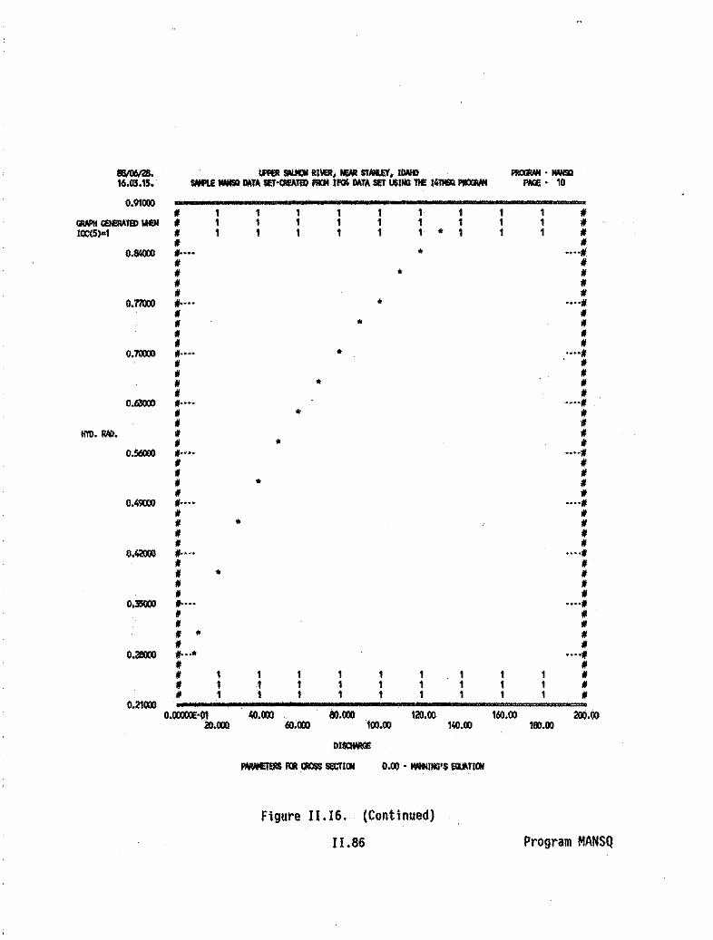
/laIlJW28,. __11\91, _ STNIEI, 1_ PRaMl'1Wl!D16.0J.15. tIH'I.E _lIIT4 $l!NJll1A1lIl 1'104 1!ll4 lIITA sa US11IB TI£ 14lll9Q PRaMl lWil • 10
0.91000II 1 1 1 1 I I I II
GIW'li _1lIl1.lEll II 1 1 1 1 1 1 1 It1~5)o1 II 1 1 1 1 1 1 • 1 II
II II.0.81000 I/o••• • ····11.
It ItII • IIIt IIII II
0.7llXXl I/o••• • ····11II IIII • IIII IIII II
0.'I\lXQ I/o ••• • ····11II IIII IIII • IIII II
O.6'lOOl ,I•••• ····11II • ItII II
HID. 1Wl. II IIII • II
O.56OCO I/o••• •..·11II 1/II ItII * IIII 11
O.4~ ..... ····11II 11II * IIII IIII II
0._ f. •.• •• ··11II II, • ItII IIII II
O.lS!XQ f. .•• ····11, 1/II IIII • IIIt II
0._ fl. ••• ••..11II ItII 1 1 1 1 1 1 , II, I 1 , 1 1 1 1 IIII 1 1 1 1 1 1 1 II
0.210000.1XKlXl!·01 CUOl ~.OOO 120.00 160.00 200.00
In.OOO 60.000 100;00 110.00 100.00
Ol~
~'IIUJ&IlS rat .QllII!l se:tllJl 0.00 • 1\IlII1NG'$ !llI\TllJl
Figure Il.16. (Continued)
11.86 Program MANSQ

ll!l/OI!oI3I. \.llP8l _ ~1\lER. _ srNUY. llWI:I _.-16.18.15. SIH'U! _ MTA lET-lll!A1lD IlQI I~ MTA lET l.$lIG TIE 14__ pu. 11
0.7lIXD • 1 , 1 I , 1 1 1 1 •__1lD1IEll • 1 1 1 I 1 1 * I 1 1 •IOC(5l'" • 1 I I I I 1 1 1 1 •• •
O.l'2OOO ..... * •••••
• ,• * •• •• * •
0.6!OOO "'H& ...,.• • •• ,, ,/I • ,
O./lXXlO ..... ....,/I ,• • ,• •/I •
O.~ ..... * .....• ,• •AVE. 0EI'IlI • ,• *
,0.4$',0) ..... ....,
• ,• *
,• ,/I ,
0.4lOOO ..... ....,/I •/I • •• •/I •0.36000 •.... .....• •, • ,, ,• •0.30000 ..... ....,• ,/I ,• ,• /I
0.24000 ..... .....• .. ,• 1 1 1 I 1 1 ,• I 1 1 I 1 1 ,, 1 I 1 I I 1 ,
0.1llXllO.OOOOE·OI 40.000 ll3.ooo 120.00 1lIO.00 3».00
lO.ooo 8>.000 100.00 140.00 1113.00
D1SClWQ!
PUlbJEIERS Fat ams SEC'flQl 0.00 • _lIG'S IlUlTlal
Figure t1.16. (Continued)
11.67 Program MAHSQ

IlIl/OI\I28. lR'Ill _ RI\Elt, _ STIlUY, lOollO ---16.l8.15. __MTA SET·MA1lIl FlllM IFIll MTA SET WIlli TIl! 14ll$:l _ PIG! • 12
MIDI • 1 , 1 1 1 , I 1 , 1/__1lIl_ • I , I I I I I 1 I /I11;1;(5)01 II 1 , 1 1 1 , • 1 I 1 iI
II •1..3J1O ..... • ····iIII /I• • /I, iI• iI
1.1100 ..... • ····iI• ,II (I
• • iIII (I
1.0400 ..... • ····iI• 1/• /I, • ,, iIO.1\!lD) 1/•••• ····iI, ,, • ,MlX._ , 1/, ,O.lIIlCXO ..... w ••• ,1/, ,, iI, ,, • ,O.tlXOO ..... ....//, (I, ,, (I, w ,0.r.mJ ..... ....,, ,
• ,(I ,II ,
0.6'000 ,.... • ....,, ,, /I, /I, ,O.SEOOIl ..... ....,, 1/, , I I 1 1 #, • 1 1 1 1 1 #, 1 1 1 1 I ,0.4lml ....
O.lXXXX"E·01 «1.(0) 00.(0) 120.00 160.00 100.0020.(0) 60.(0) 100.00 1«1.00 100.00
OlstlWltE
_ fl:ll CROOS SttTIQI 0.00 • _lNG'S ECUUIQl
Figure IL16. (Continued)
11.88 Program MANSQ

/lllIlI6I28. Il'I'ER lWIOI RIVER, HEAR srNll.Ef, 1_ PIOJWl·_16.03.15. SNf'l! _!lATA l£T·Qll;AlfD fR(M 1Fll4!lATA l£T USING nt 141lSl PImlAM PAIl: • 13
51.001
* 1 1 1 1 1 1 1 1 1 *_ lBERAlfD \olEN
* 1 1 1 1 1 1 1 1 1 *10C(5)<! * 1 1 1 1 1 1 1 1 1 ** *1t8.001 *.... ....*1# ** ** ** • *45.001 II···· • ....** *II • ** • 1#1# • #
~.OOI 1#•••• •"'1#1# • 1#
* • 1#1# 1#1# • *39.001 fl. ... ••••## • 1## 1#
WIDTH 1# ## • #
36.001 #.... ••••## ## • #
* ** #33.001 *.... ....*
# • 1#1# ** *# *30.001 *.... ..••1## • #
* #1# *# 1#
2T.00I *.... ••• -1/# 1#
* • #
* ** #24.001 ,.... •...#
# #1# 1 1 1 1 #, 1 1 1 1 ,* 1 1 1 1 #
21.001O.ll:lOO(l;·O1 40.001 00.(1)) 120.00 100.00 200.00
20.001 00.001 100.00 140.00 100.00
DISCII\'l(E
_ fQl CROSS SECTIQI 0.00 • lWJ!ING'S Ell.I\TlQl
Figure 11.16. (Continued)
1I.89 Program MAt{SQ

lI8I06I28. I,I'f9l _ RI\1ill. _ STIIIUlY. I1WO _.-16.1ll.1S. SIlFlE _ MTA SET-CllfATIl) FlQt lFG4 MTA Slrr USlll'l1llt 141MSQ _ !WE • 14
51.COO,
• 1 1 1 1 1 1 1 •(lW>If lE/EllllTll) IOIe • 1 1 1 1 1 1 1 •lCl:lS!"1 • , 1 1 1 , 1 1 •• •~.COO ,.... ....,, .. •• ,• • ,, ,
45.COO ,.... • ....•• • •• • .. •• •, • •42.COO ..... • ....,fI •, • •, ,• • ,
39.00l ..... ....•, • ,, fIl.ET. PalM. • •, • ,
36.COO ..... ....,• ,, • •• ,f1 f1
33.COO ..... ••••f1f1 • f1f1 •f1 •f1 •3O.COO ,.... ••••f1f1 • •• •f1 •f1 •
".00l fI.. •• ....•# •, • •fI ## •04.COO ,.... ••••## •# 1 1 1 1 1 1 ## 1 1 1 1 1 1 ## 1 1 1 1 1 1 •21.COO
O.llX(tt·ot 4O.COO OO.COO 120.00 160.00 200.002O.00l 6O.COO 100.00 140.00 m.oo
DISQWQ;
PNWElERS RR !HlSS SECTICll 0.00 • _11l'l'S e:ll\T1Q1
Figure 11.16. (Concluded)
11.90 Program MANSQ
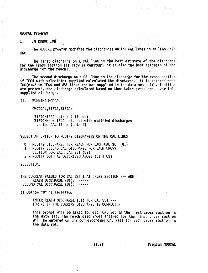
MODCAl Program
I. INTRODUCTION
The MODCAl program modifies the discharges on the CAL lines in an IFG4 dataset.
The first discharge on a CAL line is the best estimate of the dischargefor the cross section (if flow is constant, it is also the best estimate of thedischarge for the reach).
The second discharge on a CAL line is the disch~rge for the cross sectionif IFG4 with velocities supplied calculated the discharge. It is entered whenIOC(B)=Z in IFG4 and WSL lines are not supplied in the data set. If velocit.iesare present, the discharge calculated based on them takes precedence over thissupplied discharge.
II. RUNNING MODCAl
RMODCAL,ZIFG4,ZIFG4H
ZIFG4=IFG4 data set (input)ZIFG4H=new IFG4 data set With modified discharges
on the CAL lines (output)
SELECT AN OPTION TO MODIFY DISCHARGES ON THE CAL LINES
o = MODIFY DISCHARGE FOR REACH FOR EACH CAL SET (QI)1 = MODIFY SECOND CAL DISCHARGE FOR EACH CROSS
SECTION FOR EACH CAL SET (Q2)2 = MODIFY BOTH AS DESCRIBED ABOVE (QI &Q2)
SELECTION:
THE CURRENT VALUES FOR CAL SET 1 AT CROSS SECTION --- ARE:REACH DISCHARGE (Ql):
SECOND CAL DISCHARGE (Q2):
If Option ·0· is selected:
ENTER REACH DISCHARGE (Ql) FOR CAL SET --(OR -1 IF THE CURRENT DISCHARGE IS CORRECT.)
This prompt will be asked for each CAL set in the first cross section inthe data set. The reach discharges entered for the first cross sectionwill be entered on the corresponding CAL sets for each cross section inthe data set.
11.91 Program MODeAl

If Opt! on Ill" is selected:
ENTER SECOND CAL DISCHARGE (Q2) FOR CAL SET .- AT CROSS SECTION ...(OR -I IF THE CURREN~ DISCHARGE IS CORRECT)
If Option "Z" is selected:
The above two prompts will appear for the first cross section; forsUbsequent cross sections in the data set, only the prompt for bestestimate of diScharge will be asked.
11.92 Program MODCAL

MOOIoe Program
I• INTROOUCTION
The MODIOC program changes the IOC options in the following data sets(lFG4,WSP,MANSQ) and options files (HABTAT,HABTAH,HABTAV,HABVD,HABTAE).
JUST the option numbers are modified with the MODIOC program; not theassociated lines (I.e .. NOSE line, CELL line, etc.). For example, if MODIOC isused to set IOC(14)-Z in HABTAT, the user will not be prompted to enter theassociated NOSE line. Likewise, if IOC(14) is changed from "2" to "0", the NOSEline is not removed. Also, ALL options must be re-entered when changing optionsusing the MODIOe program. With the above considerations in mind, it may beeasier to use an editor to change the appropriate option(s) and lines.
II. RUNNING MODlacRMODIOC,ZIN,ZOUT
ZIK=original data set (input)ZOUT=new data set with modified options (output)
.ill DATA SET TYPE
1 HABTAT2 HARTAV3 HABTAM4 IFG45 WSP6 HABVD7 MANSQ8 HABTAE
ENTER DATA SET 10:
For example, if you wish to modify options in a WSP data set, enter "5"here. See note below for additional information on WSP options.
The options are displayed for the data set specified by the user. The user isasked to enter the laC values.
NOTE: This is the only program where the user is prompted for the additionallines required When Options 1 or 7 are "on" in WSP (CTRI and CTRF lines).Options 2,3, and 4 also require additional lines, but the user is not promptedfor the required information, as these options are not normally used in instreamflow studies. Refer to "Guide to the Application of the Water Surface ProfileComputer Program" (U.S. Bureau of Reclamation 1968) for more information on theoptions.
11.93 Program MOOIOC
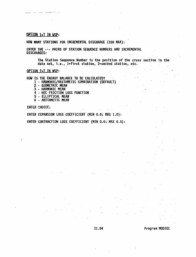
j)fi1ON 1-T IN YSP:
HOW MANY STATIONS FOR INCREMENTAL DISCHARGE (100 MAX):
ENTER THE ww. PAIRS OF STATION SEQUENCE NUMBERS AND INCREMENTALDISCHARGES:
The Station Sequence Number is the position of the cross section in thedata set, i.e., I-first station, 2-second station, etc.
OPTION 7-T IN WSP:
HOW IS THE ENERGY BALANCE TO IlE CALCULATEP?I . HARMONIC/ARITHMETIC COMBINATION (DEFAULT)2 • GEOMETRIC MEAN3 • HARMONIC MEAN4 - HEC FRICTION lOSS FUNCTION5 - ELLIPTICAL MEAN6 - ARITHMETIC MEAN
ENTER CHOICE:
ENTER EXPANSION LOSS COEFFICIENT (MIN 0.0; MAX 1.0):
ENTER CONTRACTION LOSS COEFFICIENT (MIN 0.0; MAX 0.5):
11.94 Program MODIOC

MOON Program
I. INTRODUCTION
The MOON program adds or modifies N values for each cross section in anIFG4 or WSP data set.
In an IFG4 data set, N values are supplied on the NS lines for eachsurveyed point On the cross section, in the same order as the points were givenon the coordinate lines. Although Manning's Nvalues may be supplied for allverticals, they need only be supplied at points on the cross section which areabove all measured flows and thus had no measured velocities. When Nvalues arenot suppl ied, the program calculates them for all cell s with two or more measuredvelocities. In the simulation phase when Nvalues are needed, but not supplied,the program takes the N values from the nearest cell where they were suppliedor calculated. It will also print a message in the IFG4 output file indicatingthe need for N values and count this as ,a "note". If the user does not agreewith internally generated Nvalues, he may supply his own values for subsequentruns.
In a WSP data set, Nvalues for each cell in the cross section are enteredon the Roughness lines. Amaximum of 100 Nvalues may be used per cross section.The Thalweg must be indicated with a negative sign. The Nvalues are determinedat the right hand boundary of the cell. These boundaries should be establishedat all significant breaks in the channel and floodplain geometry and atsignificant changes in microhabitat.
II. RUNNING MOON
RMODN,ZlN. lOUT
IIN-IFG4 or WSP data set (input)IOUT=modified IFG4 or WSP data set (output)
HOW ARE THE ROUGHNESS (N) VALUES TO BE MODIFIED?1 - CONSTANT REPLACEMENT2 - CONSTANT MULTIPLIER3 - DIRECT INDIVIDUAL REPLACEMENT
ENTER CHOICE:
Constant Replacement = All cells in a cross section are assignedthe Roughness (N) value supplied.
Constant Multiplier = All the Roughness (N) values for the cellsin a cross section are mUltiplied by the number supplied. Theresulting values replace the values currently on the lines.
Direct Individual Replacement =Roughness (N) values can bechanged for individual cells in a cross Section.
11.95 Program MOON

· .__ ._.. 0_- ._
The following prompt will be asked for a WSP Data Set:
ENTER 1 FOR VARIABLE REACH LENGTH, 0 FOR BLANK REACH LENGTH:
If stationing was used as cross section 10 numbering, enter '0".If station indexing was used, enter "I".
Refer to Appendix A"WSP Data Set Format· Coor9inate Lines and RoughnessLines" for discussion of stationing vs. station indexing. .
The Roughness (N) Values for each cross section are displayed and the user isprompted to enter Nvalues according to what choice was entered above.
NOTE:. In a WSP data set, the Nvalue displayed may not be the actual NvaluQ'thatis read if the Main Channel and Overbank Roughness Multipliers are set toa value other than "r" on the QARO line. .
11.96 Program MOON
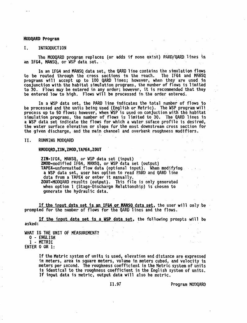
MODQARD Program
I. INTRODUCTION
The MODQARD program replaces (or adds if none exist) PARD/QARD lines inan IFG4, MANSQ, or WSP data set.
In an IFG4 and MANSQ data set, the QARD line contains the simulation flowsto be routed through the cross sections in the reach. The IFG4 and MANSQprograms will accept up to 100 QARD lines; however, when they are used inconjunction with the habitat simulation programs. the number of flows is limitedto 30. Flows may be entered in any order; however, it is recommended that theybe entered low to high. Flows will be processed in the order entered.
In a liSP data set, the PARD line indicates the total number of flows tobe processed and the units being used (English or Metric). The liSP program willprocess up to 50 flows; however, when liSP is used on conjuction with the habitatsimulation programs, the number of flows is limited to 30. The QARD lines ina liSP data set indicate the flows for which a water sUface profile is desired,the water surface elevation or slope for the most downstream cross section forthe given discharge, and the main channel and overbank roughness modifiers.
II. RUNNING MODQARD
RMODQRD,ZIN,ZMOD,TAPE4,ZOUT
ZIN=IFG4, MANSQ, or liSP data set (input)ZMOD=modified IFG4, MANSQ, or liSP data set (output)TAPE4=unformatted flow data (optional input). When modifyinga liSP data set, user has option to read PARD and QARD linedata from a TAPE4 or enter it manua'lly.
ZOUT=MOOQARD results (output). This file is only generatedwhen option I (Stage-Discharge Relationship) is chosen togenerate the hydraulic data.
If the input data set 1s an IfG4 or MANSO data set, the user will only beprompted for the number of flows for the QARO lines and the flows.
If the input data set is a liSP data set. the following prompts will beasked:
WHAT IS THE UNIT OF MEASUREMENT?o - ENGUSH1 - METRIC
ENTER 0 OR 1:
If the Metric system of units is used, elevation and distance are expressedin meters, area in square meters, volume in meters cubed, and velocity inmeters per second. The roughness coefficient in the Metric system of unitsis identical to the roughness coefficient in the English system of units.If input data is metric, output data will also be metric.
11.97 Program MOOQARO

HOW WILL THE HYDRAULIC DATA BE GENERATED?
o - CONSTANT SLOPE IS TO BE USED1- STAGE-DISCHARGE RELATIONSHIP IS TO BE USED2 - WSL AND DISCHARGE DATA WILL BE ENTERED BY USER3 - WSL AND DISCHARGE DATA IS ON A TAPE4 TYPE FILE
ENTER CHOICE:
Options 0 or 2 are usually used.
HOW MANY FLOWS FOR QARD LINES (MAX 30):
ENTER THE -- STREAM FLOWS:
ENTER A CROSS SECTION WIDTH AND A REACH LENGTH DISTANCE MULTIPLIER:
These are the multipliers entered on the PARD line when working with verylarge rivers (those over two miles wide or if the flood plain is inclUded).The maximum number allowed in a dataset Is 9999.; by using a multiplierthe actual length and width can be specified. This multiplier applies tothe Xcoordinates entered on the Coordinate Lines and the reach length onthe Roughness Lines.
If multipliers are not being used, enter "I" for both multipliers.
If "0" was entered above to yse constant slope:
ENTER CONSTANT SLOPE:
If "2" was entered above to enter WSL and discharge dat~:
ENTER THE·- WATER SURFACE ELEVATIONS:
HOW WILL THE ROUGHNESS MULTIPLIER BE DETERMINED?o = DIRECT ENTRYI = CALCULATED USING RM~(Q/QC**B)
Usually when converting an IFG4 data set to a WSP data set using theRI4TWSP procedure, "0" is entered and then "I"'s are entered as themultipliers. These are the multipl iers that are entered on the QARD lines.These roughness modifiers are changed when calibrating a WSPdata set.In the calibration phase, it may be easier to use an editor to change theroughness multipliers rather than use the MODQARD program.
11.98 Program MODQARD

•ENTER THE MAIN CHANNEL AND THE OVERBANK ROUGHNESS MULTIPLIERSFOR THE -- DISCHARGES.
ENTER A MAIN CHANNEL ANO AN OVERBANK MULTIPLIER FOR DISCHARGE --:
This prompt will appear· for each discharge specified above.
For instream flow analysis, the main channel and overbank roughnessmodifier should be set to the same value. The main channel roughnessmodifier is a factor applied to the main channel roughness coefficient togive it a desired modification. The overbank modifier is applied in thesame manner as the main channel modifier. Roughness modifiers are usefulwhen a uniform adjustment is desired for all roughness coefficients withina certain channel reach. This is a carry-over from a previous version ofWSP. As currently used, the main channel would only equal the Thalwegcell, everything else is "overbank"; this is the reason both multipliersare equal.
• 11.99 Program MODQARD

•MODSlP Program
I. INTRODUCTION
The HODSLP program modifies the slope at each cross section in an IFG4 dataset OR modifies the water surface elevation or slope for each flow on the QARDlines in aWSP data set. In a WSP data set. either the, slope or water surfaceelevation is entered on the QARD lines. If the value entered is greater than0.1, it is the water surface elevation; if the value entered is less than 0.1,it is the estimated starting water surface ,slope.
II. RUNNING MODSLP
RHODSlP,ZIN,ZOUT
ZIN=IFG4 or WSP data set (input)ZOUT-new IFG4 or WSP data set with modified slopes (output)
The two title lines from the data set will appear.
If you are modjfing an IFG4,data set:
PRESENT SLOPE FOR CROSS SECTION --- IS:ENTER NEW SLOPE OR 0 TO LEAVE AS IS:
The above prompt will be asked for each cross section in the dataset.
If you are modifying a WSP data set:
PRESENT SLOPE/W.S ELEVATION FOR FLOW OF -.- IS:ENTER NEW SLOPE/W.S. ELEVATION OR 0 TO LEAVE AS IS:
The above prompt will be asked for each flow on the QARD lines inthe data set•
•11.100 Program MODSlP ,

- change the roughness (N) values.- change Option values.- add PARD and QARD values.
QCKWSP Program
I. INTRODUCTION
The QCKWSP program creates an incomplete WSP data set (missing PARD andQARD values) from a free-formatted file created with an editor. Type INFOQWPfor information on the format of the free-formatted input file.
The roughness is assumed to be 0.035; which is described as earth channelsthat are considerably covered with small growth and cleared, but not continuouslymaintained floodways.
The following programs could be run to modify the WSP data set created byQCKWSP:
MOONMODIOCMOOQARO
Refer to Appendix Afor the file format for the. free-formatted input filefor QCKWSP; or type INFOQWP for on-line information. AppendiX A also containsa sample free-formatted input file to QCKWSP.
II. RUNNING QCKWSP
RQCKWSP,ZIN,ZWSP
ZIN~free-formatted coordinate data file (input)ZWSP=WSP data set (output)
11.101 Program QCKWSP

. -- .-. - ----_. _ __. -- _ _ - .. -.
REVI4 program
I. INTRODUCTION
TheREVI4 program assists in determining the best approach ,to hydraulicsimulation for a given site using a complete IFG4 data set. Much of thediagnostic data generated are presented as plots. The TAPE3 and TAPE4 filesgenerated can be used as input to the SLOP34 and LPTIHWE programs for furtherreview of an IFG4 data set. They are automatically used as input to theseprograms when the TREVI4 batch/procedure file is run for a ·total review· of anIFG4 data set.
Relationships between variables are determined using a log-log and semi-logrelationship. Roughness is calculated and displayed. The stage-dischargerelationship is determined and the water surface elevations determined for thestreamflow on the QARD lines. If the first QARD has a zero flow value, then thewater surface elevation is determined at the calibration flows, 0.4 and 0.2times the lowest calibrated discharge and 2.5 and 5.0 times the largestcalibration discharge. These water surface elevations are written to the TAPE4file along with the average velocity. The cross section data (i.e., distances,elevations, and channel indexes) are written to TAPE3.
II. RUNNING REVI4
RREVI4,ZIFG4,REVOUT,TAPE3,TAPE4
ZIFG4-IFG4 data set (input)REVOUT-REVI4 results (output)TAPE3-unformatted cross section and reach data (output)TAPE4-unformatted flow data (output)
. NQIf: On the microcomputer, graphs may be printed to the screen or to the outputfile using character graphics (132 characters per line format). In orderto use screen graphics, the computer must have a Color Graphics Adaptor(eGA) or compatible graphics card. When using screen graphics, notes arewritten to the output file in the positions where the graphs would havebeen placed had they been written using character graphics.
Figure 11.19 contains sample output from the REVI4 program.
III. ERROR MESSAGES
Refer to the IFG4 program description for information on error messages.
II .102 Program REVI4

DO/Ol/0s. UPPER SAlMON RIVER, NEAR STANLEr, 10ANO PROGRAM - REVI409.13.30. SAMPLE IFG4 DATA SET PAGE· 1
IOC'S ARE 0 I 0 0 1 0 0 0 0 0 0 0 1 ri 0 0 0 0 1 0o 0 000 0 0 0 000 0 0 0 0 0 0 000
METRIC INDEX IS................... 0
NUMBER OF STREAMFLOWS SINULATED IS 14
THE SIMULATED FLOIIS ARE .
8.0060.00
120.00
10.0010.00
~ 130.00
20.0080.00
30.0090.00
40.00100.00
50.00110.00
ONLY THE DATA GENERATED FOR THE FIRST CROSS SECTION IS INCLUDED IN THIS SAMPLEOUTPUT.
CROSS STATION 10 NUMBER: 0.00
WEIGHT ON SECTION WORKING UPSTREAM, 0.30
REACH LENGTH TO OOWNSTREAM CROSS SECTION, 0.00000
STAGE OF ZERO FLOW: 91.20
GIVEN SLOPE: 0.02667000
NUMBER OF COORDINATE POINTS, 30
COOROINATE OATA FOlLOWS~~~~••~.P~-~···_~ •••
OISTANCE 0.0 2.5 4.0 4.3 5.5 7.6 11.9 14.2 16.2 16.5ELOATION 101.3 100.1 99.8 98.6 91.1 97.3 97.6 97.9 97.6 97.7CHANNEL INOEX 3.0 3.0 3.0 3.0 9.2 6.0 6.0 8.2 8.2 8.2
OISTANCE 18.2 20.2 22.2 24.2 26.2 28.2 30.2 32.2 33.0 34.2ELEVATION 97.5 97.4 97.3 97.2 91.3 97.5 97.4 91.7 97.6 97.6CHANNEL INDEX 8.2 9.0 9.0 9.0 9.0 9.0 9.0 9.0 9.0 9.2
OISTANCE 35.2 36.2 37.4 39.1 43.8 53.0 62.4 69.9 16.1 67.1ELEVATION 97.7 91.7 97.7 97.9 9B.I 98.6 99.0 98.5 99.0 99.5CHANNEL INDEX 9.2 9.2 9.2 10.0 10.0 10.0 10.0 8.2 3.0 3.0
CROSS SECTlON 0.00
GIVEN FLOWCALCULATEO FLOW
STAGE
21.80 12.60 1.90l8.34 0.00 0.0097.86 97.16 91.65
VELOCITY CALlGRATlON DATA
LOCATION VELOCITIES
0.0 0.00 0.00 0.002.5 D.DO 0.00 0.004.0 0.00 0.00 0.004.3 0.00 0.00 0.005.5 0.30 0.00 0.001.6 0.00 0.00 0.00
SAMPLE VELOCITY DATA TERMINATED HERE FOR BREVITY.
Figure· 11.19. Sample output from the REVI4 program.
ILl03 Program REVI4

88/07/05.09.13.30.
UPPER SAlMON RIVER, NEAK STANLEY, IDAHOSAMPLE IFG4 DATA SET
AVERAGE CHANNEL PARAMETERS FOR CROSS SECTION 0.00
. PROGRAM - REVI4PAGE - 4
STREAM WATER SURFACE WIDTH CROSS SEC. WETTED AVERAGEFLOW ELEVATION MEA PERIMETER DEPTH
MAX PLOTTING HYDRAULIC CONVEYANCEDEPTH STAGE RADIUS FACTOR
21.812.67.9
97.8G97.7697.65
n.930.524.0
11.38.15.1
33.130.724.2
0.340.270.21
0.880.580.45
0.660.560.45
0.3420.2880.211
3.943.744.38
REGRESSION EQUATION IS -
CFAC • D.5170E+01· Q.' -0.099
STANDARD ERROR OF ESTIMATE IS
AVERAGE ERROR IS -
WIDTH. 0.1327E+02 • Q•• 0.304
DEPTH· 0.7912E-OI· Q•• 0.478
VELOCITY' 0.9S28E+00 • Q•• 0.218
0.039
4.906 PERCENT
Figure .1,19. (Continued)
11.104 Program REVI4

lJlll!R _ RIIEll, _ STNI.E\'. IIWOSAIf'l.li: 1FG4 DIoTA SET
_. REVl4
1'N1i' 5
•
100.00. ,...
,I•••II....II,I."II....II,...IIII,I• ••
IIIIII....IIIIIIIIII
01_ IIII
10.00l ,I•••••,...,...II,...II,...#I,...II,I•••
#I#I,...#I#I#I,...#I#I#I#I#I#III
1.(000a.tOOl
1
1
•
1
•
1 "·11···11
II"'11
II•"11
II"'11
II•..11,
II···11
II,,...,,,,,,IIII.....,
...,...,II
•..11,···11,...,
II...,IIII...,IIII,
···11,,,,,,1111
STAGE·STl
STAGE • 01_ DIoTA Ill! CIIOSS sa:tIQl 0.00 STl. 91.?!J
Figure 11.19. (Continued)
11.105 Program REVI4

88/01105.09.11.30.
UPPER SALMllR RIVER, REAR STAIILEY, IDAHOSAMPLE IFG4 DATA SET
CALIBRATION OF STAGE-DISCHARGE RELATIONSHIP
PROGRAM - REVl4PAGE - 6
DISCHARGE
21.80012.6007.900
STAGE
91.86097.76097.650
PLOTTING STAGE
0.6600.5600.450
STAGE OF ZERO FLOW IS 97.20
STAGE - DISCHARGE RELATIORSHIP
LOG - LOG FORcnoR
Q• 0.621E+02 '(STAGE - 91.20 )" 2.623
MEASURED PREO[CTEO RATIO21.800 20.890 1.04412.600 13.571 0.9281.900 7.651 1.013
MtAR ERROR 5.03VARIANCE 5.84
STD. DEV. 2.42SAMPLe SIZE 3.
DISCHARGE WSL VELOCITY FROUDE NUMBtR
130.00 98.53 3.40 0.67120.00 98.49 3.30 .(J.66110.00 98.44 3.20 0.65[00.00 98.40 3.0B 0.6490.00 98.35 2..97 0.6380.00 98.30 2.84 0.8270.00 98.25 2.71 0.81SO.OO 98.19 2.51 0.6050.00 . 98.12 2.41 0.5B40.00 98.05 2.24 0.5710.00 97.96 2·05 0.5620.00 97.85 1.82 0.5510.00 97.70 1.68 0.578.00 91.66 1.52 0.58
Figure 11.19. (Continued)
II.106 Program REVI4
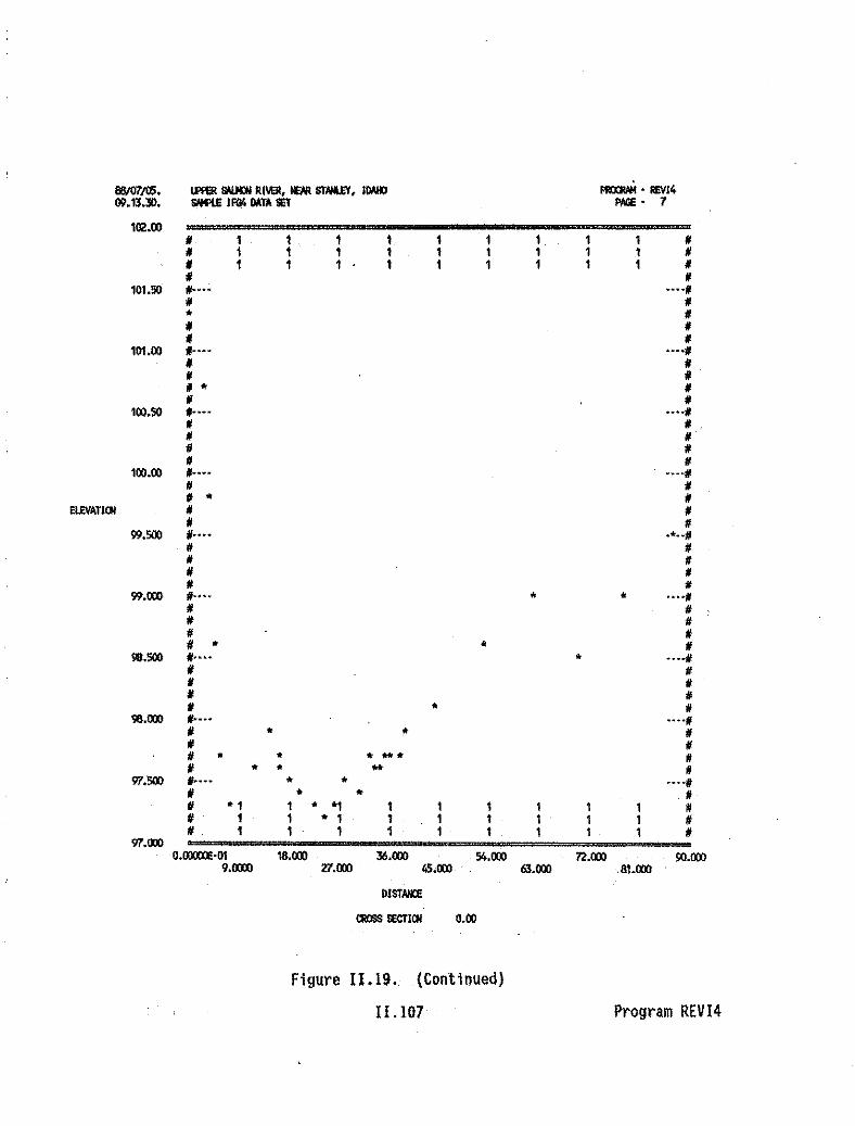
Figure 11.19. (Continued)
11.107 Program REVI4
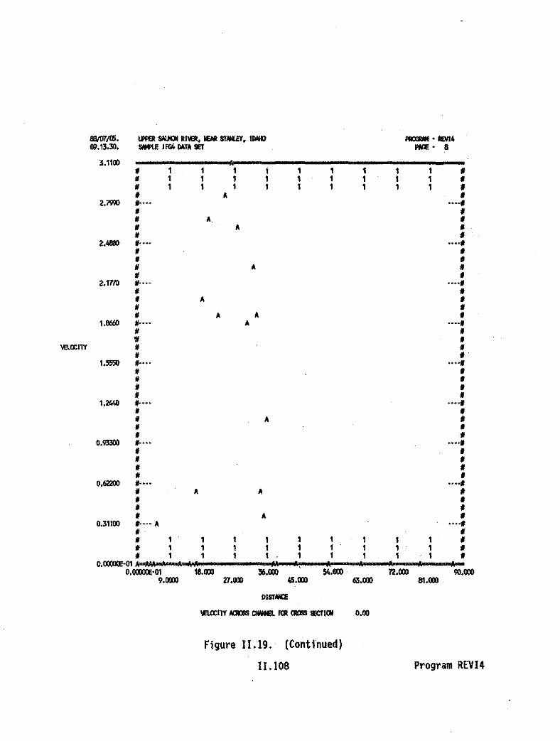
8/lIf1T/fI;. __ RI\8l. !EM SfNUl'. IIWD I'lOMl • 111;V1419.13.:10. IWl'LE JfG4 ll/.TA lET IWlE • 8
3.1100 ,, 1 1 1 , 1 1 , , I ,, 1 1 1 1 1 1 1 I I ,, 1 I 1 1 1 1 I I I ,, A ,~.19W ..... ....,, ,, A. ,, ,, ,~.- fI-'" ..",, ,, ,
• A ,II ,
~.1710 ..... .".,II ,, A ,• ,• A A ,
1.66/0 f··.. A ....,f ,'/I ,
'aOCITT , ,• ,
1,5550 ..... ....,• ,1/ ,, ,, ,
1.~ ...,. ",.,• ,, A ,, ,, ,0.9.l3OO ,..,. ..,.,, ,, ,, ,
• ,0.6ZliXl fI- ... ....,, A A ,
1/ ,, ,• A ,
0.31100 , .... A .".,, ,, 1 1 1 I 1 ,, 1 1 1 I I ,, I 1 t t I t ,O.lXII:In:-01 __
\t !" or.. 1 ;' .\n
O.OOXXl'OI 18.000 :16.000 $4.000 72.000 90.000OOסס.9 27.000 45.000 61.000 81.000
OISfNICE
IaO:ITT AallSS _ RR OIOI!B Sl'£flal 0.00
Figure n.19. (Continued)
II .108 Program REVI4

88/07/05. UPPER SALMON RIVER, NEAR STANLEY, IDAHO PROGRAM - REVl409.13.30. SAliPLE IFG4 DATA SET PAGE - 9
CROSS SECTION 0.00
GIVEN FLOI/ 21.80 12,60 7.90STAGE 97.86 97.76 97.65
CALCUlATED ROUGHNESS.*•••_~~~E.D.C~ ••••••E ......a ...~=~-====
LOCATION ROUGHNESS
0.0 0.000 0.000 0.0002.5 0.000 0.000 0.0004.0 0.000 0.000 0.0004.3 0.000 0.000 0.0005.5 0.239 0.000 0.0007.6 0.000 0,000 0.000
11.9 0.000 0,000 0.00014.2 0.000 0.000 0.00016.2 0.000 0.000 0.00016.5 0.133 0.000 0.00018.2 0.059 0.000 0.00020.2 0.055 0.000 0.00022.2 0.087 0.000 0.00024.2 0.065 0.000 0.00026.2 0.053 0.000 0.00028.2 0.048 0.000 0.00030.2 0.078 0.000 0.00032.2 0,031 0.000 0.00033,0 0.051 0.000 0.00034.2 0.177 0.000 0.00035.2 0.189 0.000 0.00036.2 0.063 0.000 0.00037.4 0.000 0.000 0.00039.1 0.000 0.000 0,00043.8 0.000 0.000 0,00053.0 0.000 0.000 0.00062.4 0.000 0.000 0.00069.9 0.000 0.000 0.00078.1 0,000 0.000 0.00087.1 0.000 0.000 0.000
Figure 11.19. (Continued)
[1.109 Program REV[4

8IlIU71fJ>. __ RI'IEll, _ STNUY. IIlNO m:llW4 • R£V1409.13.30. SNf'I.E II'Gl> MTA seT PAQ( • 10
0.3WXl11 1 1 1 1 1 1 1 I •• 1 1 I 1 1 1 1 1 •1/ 1 1 1 1 1 1 1 1 1/
• •0.27OOl ,.... ....•• /I/I •• •/I •0.2OIm ,.••• A ....•• •• •/I •• 11
0.21(00' ,1•••• ····11/I /I• 11• •/I A •0.11rol ,.... A ····11• IIII /I
PI1lllJESS II IIII II
0.15(00 ,.~ ..... ····11/I 11II II11 /I /III II
0.12lXl:l ..... ····11II IIII II/I /III •9.<lXln·(2 ,.••• ••••/1II /I •II /I /I'II 11II A A II
6.<lXln·(2 ,. ••• /I ····IiII /I /III A A II11 /III II
3.<lXln·(2 ,.••• II •• ..1111 ,II , 1 1 1 1 1 T 1 1 1/, 1 1 1 1 1 1 1 T T ,11 1 1 1 1 1 1 1 T 1 1/
0.<lXln·010.12lXl:l O.a4OOl 0.3am O.4Irol 0.6(000 0.72OOJ
O.TIrol 0.30000 O.42IlXI O.~ 0.66000
IlEI'l1l
IlEI'l1l VS IlQDfES$ fIR EIoCI! IlIl. seT, tlIllGS lIECIltII 0.00
Figure 11.19. (Continued)
11.110 Program REVl4

1!l3/fJ1Jf1S. t.m:R _ RII'Ill. _ $1_. _ _'1IIM409.13.30. SIH'Ul 1r04 MIA lET !WE' 11
O.:m» , t f f f t f 1 1 , ,, 1 1 t f f 1 1 1 1 ,, 1 f 1 f f 1 f 1 f ,, ,O.27OOJ fl. ••• ....,, ,, ,, ,, ,0.:l1OOO fl. ••• A ....,, ,, ,, ,, ,0.21(1)> fl. ••• ....,, ,, ,, ,, II ,O.1lllOO ,.... A ....,, ,, ,
RCl.U'ES$ , ,, ,O.fSln) ,.... ....,, ,, ,, A ,, ,O.l2lXn ..... ....,, ,, ,, ,, ,9.tmxl;·02 , •••• ....,, A ,, II ,
/I /I, II A ,6.tmxl;.(l! ..... A ....,, A II /I, A A ,, ,, ,3.tmxl;·(l! fl. ••. A ....,, ,, 1 f 1 f f f 1 f ,, 1 1 1 t 1 f f f ,, f t f t f f f t ,O.o:nn::-011frrtN h t I'd tt ... at A . 1\ 14
0.tmxl;·01 ta.(I» 36.(1)> 54.(1)> 1'2.(1)> 1'Il.o:n9.0(1)> Z1.(I» 4S.(I» 6S.(I» st.(I»
DlsrNa
IIUHESS N:lI:lSS lllJIllEI. fIJI ClOSS ElICli 0.00
Figure II. 19. (Continued)
ll.lll Program REVI4
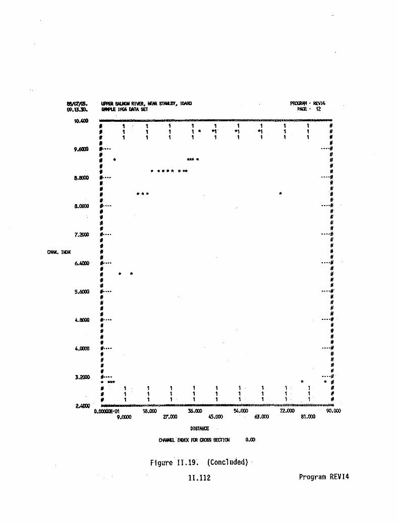
11JII11/fT>. lAlIll _ RIIIER. HEM SfNIEI. llWD PROOlIII • 1lIM4OO.~ Il'lfU llG4 lIo\TA seT !WE • 12
10.@/I 1 1 1 1 1 1 1 1 N/I 1 1 1 1 • "1' -, ., 1 N/I 1 1 1 1 1 1 1 1 N/I N
9mJ1l ......h ····N/I II/I • .... II/I 1/1/ ........ *_ • ... N
a,an) •••• ····11/I 1/1/ NII ••• • 1/II 1/
8.0XIJ .... ••••1/1/ 1/1/ 1/1/ II/I II
7.2lXXI •••• ••••1//I II1/ N
awl. IIOlC /I N/I N
MOOO •••• ····11/I II1/ • • IfII /I1/ II
$.6003 f-••• ..··N/I 1/, II/I /III ,
4._ •••• ....,1/ 1/, ,, II, ,
4.1XJ:lJ 1/.... ....•/I IIII II/I IIII II
3.2lXXI .... ····11.- • • •II I I 1 1 1 1 1 ' N1/ I 1 1 I 1 1 1 N/I 1 1 1 1 1 I 1 ' N
2,~
O.CXIIIIXl!·01 18.(0) 36.(0) 54.(0) 72.(0) 90,(0)9.0XIJ 27.(0) 45.(0) 61.(0) 81,(0)
DI6TNa
(lWHil'11IlEX fOl QlOOS !ECTIQl 0.00
Figure 11.19, (Concluded)
11.112 Program REVI4

RI4TWSP Batch/procedure File
I. INTRODUCTION
The RI4TWSP batch/procedure file converts an IFG4 data set to a completeWSP data set by running the following three programs: STRIPC, CWSPN, and MODQARD.Each vertical becomes· the right boundary of a cell, except the left-mostvertical.
II. RUNN1NG THE RI4TWSP BATCH/PROCEDURE FILE
RI4TWSP,ZIFG4,ZWSP,TAPE4.Z0UT
ZIFG4=IFG4 data set (input)ZWSP-WSP data set (output)TAPE4-unformatted flow data (optional input)
If not supplied, data for" the PARD and QARD linesare entered from the keyboard.
ZOUT-MODQARD results (output). This file is only generatedwhen Option 1 (Stage-Discharge Relationship) is chosen togenerate the hydraulic data.
Refer to the individual program documentation for STRIPC, CWSPN, and MODQARDfor more information.
,r
11.113 Batch/Procedure RI4TWSP
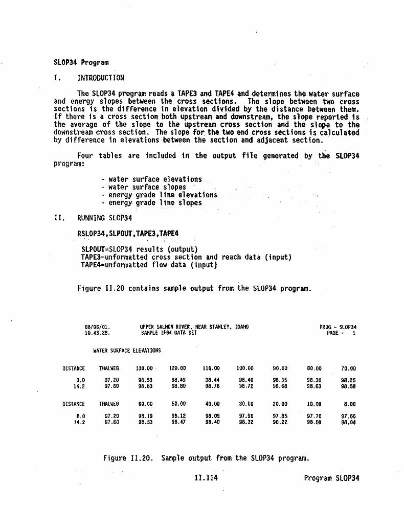
SLOP34 Program
I. INTRODUCTION
The SLOP34 program reads a TAPE3 and TAPE4 and determines the water surfaceand energy slopes between the cross sections. The slope between two crosssections is the difference in elevation divided by the distance between them.If there is a cross section both upstream and downstream, the slope reported isthe average of the slope to the upstream cross section and the slope to thedownstream cross section. The slope for the two end cross sections is calculatedby difference in elevations between the section and adjacent section.
Four tables are included in the output file generated by the SLOP34program:
- water surface elevations- water surface slopes- energy grade line elevations- energy grade line slopes
II. RUNNING SLOP34
RSLOP34,SLPOUT,TAPE3.TAPE4
SLPOUT=SLOP34 results (output)TAPE3=unformatted cross section and reach data (input)TAPE4=unformatted flow data (input)
Figure 11.20 contains sample output from the SLOP34 program.
B8/06/0!. UPPER SALHON RIVER, HEAR STANLEY, IDAHO PROG - SLOP3410.43.2B. SAMPLE IF64 DATA SET PAGE - I
VATER SURFACE ELEVATIONS
DISTANCE THALVEG 130.00 . 120.00 liD. 00 100.00 90.00 BO.OO 70.00
0.0 97.20 98.53 98.49 98.44 98.40 98.35 98.30 98.2514.2 97.60 98.83 98.80 96.76 98.72 98.68 98.63 98.58
DISTANCE THALWEG 60.00 50.00 40.00 30.00 20.00 10.00 8.00
0.0 97.20 98.19 98.12 98.05 97.96 97.85 97.70 97.6814.2 97.60 98.53 98.47 98.40 98.32 98.22 98.08 98.04
Figure 11.20. Sample output from the SLOP34 program.
11.114 Program SLOP34

88/06/01, UPPER SALHOH RIVER, NEAR STANLEY, IDAHO PROG • SLOP3410.43.28. SAMPLE IFG4 DATA SET PAGE· 2
WATER SURFACE SLOPES
DISTANCE THALIIEG 130.00 120.00 lIO.OO 100.00 90.00 80,00 70.00
0.0 97.20 0.02172263 0.02200264 0.02229496 0.02260014 0.02292084 0.02326028 0.0236211414.2 97.60 0.02172263 0.022002G4 0.02229496 0.02260014 0.02292084 0.02326028 0.02362114
DISTANCE ' THALWEG 60.00 50.00 40.00 30.00 20.00 10.00 8.00
0.0 97.20 0.02400770 0.02442798 0.02489056 0.02541311 0.02602668 0.02680942 0.0270043114.2 97.60 0.02400770 0.02442798 0.02489056 0.02541311 0.02602668 0.02680942 0.02700431
SLOPES CALCULATED USING AVERAGE OF ADJACENT SLOPES
ENERGY GRADE LINE ELEVATIONS
DISTANCE THALWEG 130.00 120.00 110.00 100.00 90.00 80.00 70.00
0.0 97.20 98.t2 98.67 98.62 98.56 98.50 98.44 98.3714.2 97.60 99.05 99.00 98.95 98.90 98.85 98.79 98.73
DISTANCE THALWES 60.00 50.00 40.00 30.00 20.00 10.00 8.00
0.0 97.20 98.30 98.22 98.13 98.03 97.91 97.74 97.7014.2 97.60 98.66 98.59 98.50 98.40 98:28 98.l! 98.07
SLOPE OF ENER6Y GRADE LINE
DISTANCE THALWES 130.00 120.00 lIO.OO 100.00 90.00 80.00 70.00
0.0 97.20 0.02278344 0.02314089 0.02351031 0.02388241 0.02425880 0.02463948 0.0250249514.2 97.80 0.02276344 0.02314089 0.02351031 0.02388241 0.02425880 0.02463948 0.02502495
DiSTANCE THALWEG 60.00 50.00 40.00 30.00 20.00 10.00 8.00
0.0 97.20 0.02541525 0.02578146 0.02591478 0.02591424 0.02596992 0.02582483 0.0258714114.2 97.60 0.02541525 0.02578146 0.02591478 0.02591424 0.02596992 0.02582483 0.02587141
SLOPES CALCULATED USING AVERAGE OF ADJACENT SLOPES
Figure II.20. (Concluded)
II. 115 Program SLOP34

STGQS4 Program
I. INTRODUCTION
The STGQS4 program determines water surface elevations for an IFG4 dataset using the stage-discharge relationship based on flows on the CAL lines. Theoutput is shorter and easier to read than IFG4 output when you are onlyinterested in the predicted water surface elevations.
Only two of the IOC values in IFG4 are used in STGQS4; they are IOC(5) andIOC(20). IOC(20) indicates that the cross section width is to multiplied by aconstant and works exactly as in IFG4. IOC(5) works a little different in STGQS4than in IFG4. If IOC(5)~O in STGQS4, the. second discharge on the CAL line isused in developing a stage-discharge relationship. If the second discharge isblank or zero, the first discharge will be used. STGQS4 does not calculatedischarges from the velocities on the VEL lines (use the values fromREVI4).If IOC(5)~1 in STGQS4, the first discharge on the CAL line. is used and must besupplied.
II. RUNNING STGSQ4
RSTGQS4,ZIFG4,ZOUT,TAPE3,TAPE4
ZIFG4~IFG4 data set (input)ZOUT-STGQS4 results (output)TAPE3-unformatted cross section and reach data (output)TAPE4~unformatted flow data (output)
Appendix Acontains the IFG4 data set that was used to generate the outputin Figure 11.21. Review the output file for error messages and inconsistanciesin data. Error messages in the form of notes or other statements may be writtenthat did not appear on the screen or cause the program to abort.
88/04/26.15.16.40.
UPPER SALKOK RIVER, KEAR STAKLEY, 10AijOSAMPLE IFG4 DATA SET
PROGRAM - STGQS4PAGE - 2
STATION ID IS 0.00
REACH LENGTH UOWKSTREAM IS 0.00 WEIGHT ON SECTION IS 0.30STAGE OF ZERO FLOW IS 97.20 GIVEN SLOPE IS 0.02667000
COORDINATE DATA FLOWS - THERE ARE 30 POINTS
DISTANCE O. 2. 4. 4. S. 8. 12. 14. 16. 16.ELEVATION 101.30 100.70 99.80 98.60 97.10 91.30 97.60 91.90 97.60 91.10
DISTANCE 18. 20. 22. 24. 26. 28. 30. 32. 33. 34.ELEVATIOK 91.50 97.40 97.30 97.20 91.30 97.50 97.40 91.70 97.60 91.60
OISTARCE 35. 36. 37. 39. 44. 53. 62. 70. 78. 81.ELEVATION 97.10 97.70 91.70 97.90 98.10 98.60 99.00 98.50 99.00 99.S0
Figure 11.21. Sample output from the STGQS4 program.
11.116 Program STGQS4

88/04/26.15.16.40.
UPPER SALMOR RIVER. NEAR STANLEY. IDAHOSAMPLE IFG4 DATA SET
CALIBRATION OF STAGE • DISCHARGE RELATIONSHIP
PRDBRAM - STOOS4PAGE - 3
DISCHARGE
21.800II.6007.900
STAGE
97.86097.16091.650
PLOTTING STAGE
0.6600.5600.450
STAGE OF ZERO FLOW IS 97.20
STAGE . DISCHARGE RELATIONSHIP
LOG • LOG FUNCTION
Q• 0.611E+02 "(STAGE· 97.10 1** 2.623
MEASUREDII. 80012.6007.900
PREDICTED20.89013.5777.651
RATIO1.0440.9281.033
MEAR ERROR 5.03VARIANCE 5.84
STD. OEV. 2.42SAMPLE SIZE 3.
DISCHARGE lISL VELOCITY FROUllE NUMBER
8.00 97.66 1.52 0.5810.00 97.10 1.58 0.5120.00 91.85 1.82 0.5530.00 97.96 2.05 0.5640.00 98.05 2.24 0.5750.00 98.12 2.41 0.5860.00 98.19 2.57 0.6070.00 98.15 2.71 0.6180.00 98.30 2.84 0.6290.00 98.35 2.97 0.63
100.00 98.40 3.08 0.64110.00 98.44 3.20 0.65110.00 98.49 3.30 0.66130.00 98.53 3.40 0.67
ONLY THE OUTPUT FROM CROSS SECTION 0.0 IS INCLUDED IN THIS SAMPLE OUTPUT.
Figure II .21. (Concluded)
H.Il7 Program STGQS4

STRIPe ProgroI. INTRODUCTION
The STRIPC program removes all but the two title lines and the coordinatelines from either an IFG4 or WSP data set. It is used when converting a dataset from either IFG4 format to WSP format or WSP format to IFG4 format.
II. RUNNING STRIPC
RSTRIPC,ZIN,ZOUT
ZIN-IFG4 or WSP data set (input)lOUT-coordinate data set (output)
When stripping an IFG4 data set, the following prompt appears to allow theuser to change the cross section 10 numbering from consecutive numbering tostationing. AWSP data set uses stationing as cross section 10 numbering.
,DO YOU WISH COLUMNS 2-10 OF THE COORDINATE SET TOCONTAIN THE ACCUMULATIVE REACH LENGTH, OR LEAVE ITUNCHANGED?
o - ACCUMULATIVE REACH LENGTH (STATIONING)I - LEAVE UNCHANGED
ENTER 0 OR 1:
ILIl8 Program STRIPe

TREVI4 Batch/Procedure File
I. I~TRODUCTIO~
The TREVI4 batch/procedure file generates files for a total review of anIFG4 data set by running the CKI4. REVI4. lPTTHWE. and SlOP34 programs. TheTAPE3 and TAPE4files are generated by the REVI4 program and are then used asinput to the lPTTHWE and the SlOP34 programs.
II. RUNNING THE TREVI4 BATCH/PROCEDURE FilE
TREVI4.ZIFG4.CKOUT.REVOUT.lPTOUT,SLPOUT.TAPE3,TAPE4
ZIFG4~IFG4 data set (input)CKOUT~CKI4 results (output)REVOUT=REVI4 results (output)lPTOUT=LPTTHWE results (output)TAPE3=unformatted cross section and reach data (output, input)TAPE4=unformatted flow data (output. input)
Refer to the individual program documentation for the CKI4. REVI4. LPTTHWE.and SLOP34 programs for sample output.
11.119 Batch/Procedure TREVI4

VWTHW£G ProgramI. INTRODUCTION
The VWTHWEG program plots Thalweg values and water surface elevations froma TAPE3 and TAPE4 as lPTTHWE does; however VWTHWEG allows the user to choose thecross section or discharge to be plotted vs. plotting all of them.
VWTHWEG uses screen graphics and is only available on the micro. Thecomputer must have a Color Graphics Adaptor (CGA) or compatible graphics card.
II. RUNNING VWTHWEG
RVWTHWEG.ZOUT.TAPE3.TAPE4
ZOUT=VWTHWEG results (output)Graphs are displayed on the screen. and the information foreach requested graph is written to the output file.
TAPE3=unformatted cross section and reach data (input)TAPE4=unformatted flow data (input)
ENTER 0 TO PLOT WSL VS. LONGITUDINAL DISTANCE FOR ACROSSSECTION. OR
1 TO PLOT THALWEG VS. WSL VALUES FOR ADISCHARGE, OR2 TO EXIT PROGRAM:
If "0" is entered to plot WSl vs. longitudinal distance for a cross section:
THE CROSS SECTIONS ARE:
1: (first Cross Section 10 No.) 2: (second Cross Section 10 No.)
Each Cross Section 10 No. on the TAPE3 will be listed preceeded witha consecutive Index number.
ENTER INDEX NUMBER OF CROSS SECTION 10 FOR GRAPH:
The index number, NOT the Cross Section 10 No. is entered, i.e ••"I" would be entered to plot the first cross section listed.
If "I" is entered to plot Thalweg vs. WSL values for a discharge:
The discharges will be listed along with an index number as explainedabove. The user will be prompted to enter the Index Number of thedischarge to be graphed.
11.120 Program VWTHWEG

WSEI4 Program
I. INTRODUCTION
The WSEI4 program reads water surface elevations and discharges from aTAPE4 or TP4 and adds or replaces the QARO and WSL lines 1n an IFG4 dataset.The original IFG4 data set must contain NS lines, as the WSEI4 program searchesfor the NS lines and inserts the WSl lines after them.
II. RUNNING WSEI4
RWSEI4,ZlFG4,ZlFG4N,TAPE4
ZIFG4-IFG4 data set {input}ZIFG4H=new IFG4 data set with added or replaced water surfaceelevations and discharges (output)
TAPE4=unformatted flow data {input}
REVIEW IOC VALUES - IOC(8} MUST BE 1 OR 3
IOC(S}=l in an IFG4 data set instructs the IFG4 program to read the watersurface elevations supplied on the WSL lines for each flow entered on the QARDlines.
IOC(S}=3 in an IFG4 data set instructs the IFG4 program to read the watersurface elevations supplied on the WSl lines for each flow entered on the QARDlines. The flow used to adjust the velocities is multiplied by the ratio ofthe discharge calculated from the velocities on the VEL lines to the dischargeon the CAL line. If more than one set of VEL lines is present. the ratio basedon the last set is used.
IU21 Program WSEI4

WSEI40 ProgramI. INTRODUCTION
The WSEI4D program adds or replaces QARO and WSl lines in an IFG4 data set.Data is entered from the keyboard. It can be used when water surface elevationsdetermined from one model are being used for some cross sections, and othermodels are used for other cross sections, or when water surface elevations fromdifferent models for individual cells in a cross section are being added to theIFG4 data set.
The original IFG4 data set must contain NS lines, as the WSEI4D programsearches for the NS lines and inserts the WSl lines after them.·
II. RUNNING WSEI40
RWSEI4D.ZIFG4.ZIFG4N
ZIFG4;IFG4 data set (input)ZIFG4N~new IFG4 data set wth added or replaced water surfaceelevations and discharges (output)
HOW MANY QARD FLOWS ( MAX 30 )(FOR NO CHANGE IN THE QARD FLOWS ENTER A 0)
If "0" is entered, the new data set with WSL lines added will contain thesame flows on the QARD lines as the original data set.
ENTER WATER SURFACE ELEVATIONS FOR THE FOLLOWING FLOWS:
If "0" was entered above for no change in the QARD flows, the existing QARDflows will be listed here.
ENTER --- WSl('s) FOR CROSS SECTION ---:
Awater surface elevation is entered for each cell in the cross section.
REVIEW IOC VALUES - IOC(8) MUST BE 1 OR 3
IOC(8)~1 in an IFG4 data set instructs the IFG4 program to read the watersurface elevations supplied on the WSl lines for each flow entered on the QARDlines.
IOC(8)=3 in an IFG4 data set instructs the IFG4 program to read the watersurface elevations supplied on the WSl lines for each flow entered on the QAROlines. The flow used to adjust the velocities is multiplied by the ratio ofthe discharge calculated from the velocities on the VEL lines to the dischargeon the CAL line. If more than one set of VEL lines is present, the ratio basedon the last set is used.
II.122 Program WSEI4D

WSEI4H Program
I. INTRODUCTION
The WSEI4H program reads water surface elevations and discharges from aHEC2 output file and adds or replaces the QARD and WSL lines inan IFG4data,set.The original IFG4 data set must contain NS lines, as the WSEI4H program searchesfor the NS lines and inserts the WSL lines after them.
The water surface elevations and discharges are read from the "SummaryPrintout" in the,HEC2 output file. The following code numbers must be selectedon Job Control Parameter Card 3 (J3) when running HEC-2 in order to generate the"Summary Printout" in the right format.
Code~ Nymber Description
I2345
6
7
89
10
3843
I45
6
7
810
Cross section identificationn numberDischargeComputed water surface elevationCross section width at calculated water surface elevationSlope of the energy grade line for the current section(time 10,000)Travel time from the first cross section to the presentcross sectionCumulative volume of water in the stream from the firstcross section in acre-feetDepth of flowMean velocity head across the entire cross sectionBlank
II. RUNNING WSEI4H
RWSEI4H,ZHECOUT,ZIFG4,ZIFG4N
ZHECOUT~HEC2 line printer output file (input)ZIFG4~IFG4 data set (input)ZIFG4N=new IFG4 data set with added or replaced water surfaceelevations and discharges from ZHECOUT (output)
REVIEW IOC VALUES - IOC(8) MUST BE 1 OR 3
10C(8)=1 in an IFG4 data set instructs the IFG4 program to read the watersurface elevations supplied on the WSL lines for each flow entered on theQARDlines.
IOC(8)~3 in an IFG4 data set instructs the IFG4 program to read the watersurface elevations supplied on the WSL lines for each flow entered on the QAROlines. The flow used to adjust the velocities is multiplied by the ratio ofthe discharge calculated from the velocities on the VEL lines to the dischargeon the'CAL line. If more than one set of VEL lines is present, the ratio basedon the last set is used.
11.123 Program WSEI4H
\lSEI4$ Program
I. INTRODUCTION
The WSEI4S program uses a stage-discharge relationship to calculate watersurface elevations which are then added to an IFG4 data set. The user entersthe stage-Q data needed to determine the stage-discharge rel ationship. Theoriginal IFG4 data set must contain NS lines. as the WSEI4S program searches forthe NS lines and inserts the WSL lines after them.
Running STGQS4 or IFG4 on a single velocity data set produces the same sameresults as WSEI4S.
II. RUNNING WSEI4S
RWSEI4S,ZIFG4,ZIFG4N.ZOUT
ZIFG4=IFG4 data set (input)ZIFG4N=new IFG4 data set with WSL lines added (output)ZOUT=WSIE4S results. stage-discharge relationship,
and plots (output) ,
On the microcomputer, graphs may be printed to the screen or to the outputfile using character graphics (I32 characters per line format). In orderto use screen graphics, the computer must have a Color Graphics Adaptor(CGA) or compatible graphics card. When using screen graphics, notes arewritten to the output file in the p<>sitions where the graphs would havebeen placed had they been written using character graphics.
HOW MANY SIMULATION (QARD) FLOWS:
ENTER THE --- FLOWS:
The following sequence of prompts will pe asked for each cross section in theIFG4 data set.
ENTER FIRST CROSS SECTION ID NUMBER:
HOW MANY STAGE - DISCHARGE PAIRS:
ENTER THE STAGE. DISCHARGE PAIRS (STQ.Q):
ENTER STAGE OF ZERO FLOW:
STAGE Q EQUATION IS
ENTER WSl AND STAGE PAIR:
This Is when the datum for the water surface elevations is not the sameas the datum ·used for the rest of the measurements. If the same datum wasused. enter two (2) equal numbers here.
11.124 Program WSE14S

- - - CALCULATING, PLEASE WAIT ---
REVIEW IOC VALUES - IOC(8) MUST BE 1 OR 3
IOC(8)~1 in an IfG4 data set instructs the IfG4 program to read the watersurface elevations supplied on the WSL lines for each flow entered on the QAROlines. ..
IOC(8)v3 in an IFG4 data set instructs the IFG4 program to read the watersurface elevations supplied on the WSl lines for each flow entered on the QARDlines. The flow used to adjust the velocities is multiplied by the ratio ofthe discharge calculated from the velocities on the VEL lines to the dischargeon the CAL line. If more than one set of VEL lines is present, the ratio basedon the last set is used.
Figure 11.22 contains sample output from the WSEI4S program. Only thestage-discharge data and plot for cross section 0.0 has been included in thisfigure.
88/05/31.12.58.57.
UPPER SALMON RIVER, NEAR STANLEY, IDAHOSAMPLE [FG4 DATA SET
PROGRAM - WSEl4SPAGE - 2
o[SCHARGE
21.80012.6007.900
STAGE
97.86097.76097.650
PLOTTING STAGE
0.G600.5600.450
STAGE OF ZERO FLOW IS 91.20
STAGE - O[SCHARGE RELATIONSHIP
LOG - LOG FUNCTION
Q• 0.62IE+02 '(STAGE - 97.20 ).. 2.623
MEASURED PRED[CTED RATIO21.800 20.890 1.04412.600 13.577 b.9287.900 7.651 1.033
MEAN ERROR S.03VARIANCE S.64
STD. DEV. 2.42SAMPLE SIZE 3.
DISCHARGE STAGE WSL
8.0 97.658 97.65820.0 97.849 97.64940.0 96.046 98.046GO.O 98.167 98.18780.0 98.301 98.301
Figure 11.22. Sample output from the WSEI4S program.
II.125 Program WSEI4S

Figure 11.22. (Concluded)
II.l26 Program WSEI4S

WSP Program
I. INTRODUCTION
The Water Surface Profile (\liSP; also referred to as IFG2) program is a U.S.Bureau of Reclamation (USBR) program modified to calculate the velocities andwater surface elevations required as input to the habitat simulation programs.WSP provides very detailed depth and transverse velocity information. The modelcan be used to predict the horizontal distribution of depth and mean columnvelocity over a range of streamflows with one set of field data.
The objective of this type of hydraulic simUlation is to be able to predicthow the depth, velocity, and widths vary for each cross section over a range ofsimulated discharges. Specific hydraulic relationships between the physicalchannel and discharge must be met to evaluate these changes in reference to astream reach.
Several basic assumptions are made in the development of the water surfaceprofile. Included are the assumptions that steady flow conditions existed duringthe period the field measurements were made and that the boundary conditionsremained rigid.
WSP requires a minimum of one (more are desirable) cross sectionmeasurement, with one water surface elevation for each cross section measuredat that flow. The program was originally intended to yield the water surfaceprofile as the end result; however, in the PHABSIM system, the end result is aset of velocities for each cross section and the water surface profiles.Application of the WSP program requires calibration of the data set for aparticular site. Care must be taken to ensure an accurate calibration becausethe results affect the calculation of habitat. Figure 11.23 flowcharts thesteps in calibrating a \liSP data set. .
Typically, the weighted usable area predicted by the habitat simulationprograms is much more sensitive to ·errors in the velocities than errors in thewater surface elevations.
Refer to Figure 11.2 for a flowchart of the various methods available tocreate a \liSP data set. For information on What each I ine in the data setcontains, instructions for entering data, and a sample \liSP data set, refer toAppendi x A - "\liSP Data Set Format".
There are several hydraulic options available in the \liSP program; however,most of them have a limited usefulness with PHABSIM. The options are summarizedbelow in Table 1[,4. For a detailed explanation of the options, refer to "Guideto the Application of the Water Surface Profile Computer Program" (U.S. Bureauof Reclamation 1968).
II .127 Program \liSP

CAUBRATING AWSP DATASET
repeat un1lf WSL~ealibralad
MOOQARD or edlto< (add additionalcalibration flows 10 OARD lines and
"''''''Sa ooughoess modllle", foraddiliooal calibration flows)
WSP Dala Sa, withcalibrated·N vaJues'0< tirot calibration
flow
MODI'l(cl1ang& II values)WSP
___ repeat until WSL~ealibrab:ld
~
~
......,ex:>
CollbIaled WSPData Set
PIotcaibralion discharges..."'"9_modifi... on
Iog-Io9 paper
MOllQARl) (&dd ,1"'01__ ...gas, WSL'O.and
roughness _IS)WSP
-0
6""-s'";3..:V>-0 figure 11.23. Calibrating a WSP Data Set.
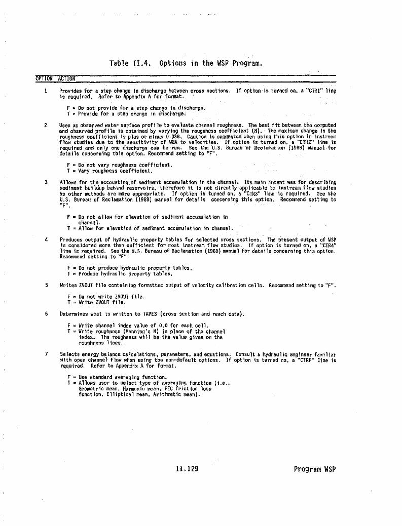
Table 11.4. Options in the WSP Program.
OPTI 011 ACTioN
1 Provides for s step change In discharge between cross ,ections. If option Is turned on, • "CTRI" 11neIs required. Refer to Appendix Afor format.
F = 00 not provide for a atep change in discharge.1 ~ Provide for 6 step change in discharge~
2. Uses an observed water surface proflle to evaluate channel roughness. The best fit betwean the computedand observed profile is obtained by varying the roughness coefficient (N). The maximum change 'n.theroughness coeffioient is plus or minus O.D36. Caution is suggested when using this option in instreamflow studies due to the sensitivity of WUA to veloctties. If option 1s turned on. a "CiRZ" line: lsrequired and only Qnedischarge ean ber-un. See the U.S. Bureau of Reclamation (19M) manua1fordetails concerning this option. Rec()tTtllend setting to "F".
F ~ Do not vary roughness coefficient.T » Vary roughness coefficient.
3 Allows for the accounting,of sediment accumulation in the ctlanneL Its main intent was for describingsed1ment buildup behind reservoirs. therefore it is not directly applicable to tnstream flow studiesas other methods are more appropriate. If option is turned on. a "CTR3" line is required. See theU.S. Bureau of Reclamation (196B) manual for details concerning this option. Recommend setting to"F".
F =Do not allow far elevation of sediment accumulatiDn inchannel. .
T =Allow for elevation of sediment accumulation in channel.
4 Produces output of hydraulic property tables for selected cross sections. The present output of ~SP
is cons idered more than stiff tcient for most instream flow studies. If opt ion is turned on f a I'CTR4"Hne is requ1red. Sea the U.S. Bureau of Reclamation (l9SS) manual for details concerning thts option.RecOSTmend setting to "F".
F ~ 00 not produce hydraulic property tables.T =Produce hydraulic property tab1es.
5 Writes ZVOUT file conta in Ing formatted output of ve loeity Cdllbrat Ion ce 11s. Recamnend sett ing to "ft•.
F • Do not write <VDur file.T • Write <VOUT file.
6 Determines what is written to TAPE3 (cross section and reach data).
F =Write channel index value of 0.0 for each cell.T • Write roughness (Manning', H) In place of the channel
index. The roughness will be the value given on theroughne$$ lines.
7 Selects energy balance ca.lculations. parameters. and equations. Consult a hydrauliC! engineer familiarwith open channel flow when using the non~default options. If option is turned on. a "ClRF" line- isrequired. Refer to Appendix Afor format.
F • Use standard averaging function.r • Allows user to select type Gf averaging function (t.e .•
Geometric mean, Harmonic mean, HEC f~iction lossfunction f Elliptical mean, Arithmetic mean).
II ,129 Program WSP

Table 11.4. (Concluded)
opTIoN AcllOll
8 Overrides certain error proces.lng by .llowing a limit on tho allowable chango in enorgy 10•• betweentwo seotiDnS: to be overriden. WSP wtll not. calculate the ups:treamwater surface elev.at1on if thech.nge in .lovatlon Is larger than a specified amount and will not procood further. Sometl~. It I.useful to review the results with a large chbnge 1n water surface elevation between two croS$. sections.
F ~ Do not ove~r1de error processing. Production run$.hould be done with thl. option off a. the underlyingproblem .hould be dealt with flr.t.
T =OVerride. limit on allowabl. change In energy 10"between two sections.
9 Writ•• the calculated .lope to TAPE4 a. an additional varlablo. If thl. option I•••l.cted. do notu.e the TAPE4 file a. Input to tho habitat .lmulatlon.prD9ram••
F =00 not wrlto calculatod .lope to TAPE4.T • Write calculated slope to TAPE4.
10 Prints out cell details in the \rISP output. Recoornend s~tting to "r" for calibration runs and oTt" for:produotion runs.
F =Print c.ll dotall •.T =00 not print cell dotall•.
NOTE; Refer to Appendix A . "WSP Data Set Format . PARD line" for informationon the critical constraint option.
Ir.130 Program WSP

II. RUNNING WSP
RWSP.ZWSP.ZOUT.TAPE3.TAPE4,TP4.ZVOUT
ZWSP-WSP data set (input)ZOUT~WSP results (output)TAPE3=unformatted cross section and reach data (output)TAPE4=unformatted flow data (output)TP4-rearranged TAPE4 file. Used as input to HABTAT (output)ZVOUT",optional output file formatted for easy review ofvelocities. Created when option 5 is on. (output)
DO YOU WANT A SUMMARY OF STATISTICS FOR CALIBRATION? (YES OR NO):I
Entering YES will run the LSTWSL program which lists the simulated watersurface elevations from the generated output file to the screen or to anoutput file to be used in the calibration process.
The TAPE3 resulting from a WSP run d~es not contain channel index values.
Channel index values are not included in a WSP data set; thus they are notpassed onto the TAPE3. Therefore, if the TAPE3 is going to be. used asinput to the habitat simulation programs, then channel index data must beadded using the MODCI program.
Channel index values are used in the calculation of Weighted Usable Area(WUA) in habitat simulation. If all the channel index values are set tozero (0), the user can set an option in the habitat simulation programsthat will either I,lse a value of channel index value of zero in thecalculation of WUA for that cell, or not use a channel index value of zeroin the calculation of WUA for that cell (i.e., only use velocity timesdepth) .
WSP does not write a TAPE4.A or TP4A which can be used as input toHABTAM orHABTAV.
Appendix Acontains the WSP data set that was used to generate the outputin Figure 11.24, Review the output file for error messages ·and inconsistanciesin data. Error messages in the form of notes or other statements may be writtenthat did not appear on the screen or cause the program to abort.
Below is a definition of the variables that may be written to WSP output.Not all of these variables are in the output for each cross section, but areusually located somewhere in the output from a WSP run.
HFl '"HF2 '"HVI '"HV2 '"HSF -
Total Head '"
Head loss for downstream section.Head loss for upstream section.Velocity head for downstream section.Velocity head for upstream section.Slope of the energy grade line at the section.Total head loss between sections.
11.131 Program WSP

89/01/09. TAYLOR RIVER IfG4. 3 fLO~S Of 162,2S4,AHO 591 ers HIGH FLOW SET,NMAXO.I0 PROGRAM-WSP(IFG2)1£;.54.18. SAMPLE CALI8RATED WSP DATA SET PAGE 2
WSP - - INPUT CONTROL LINE AND ERROR LISTING
PARD 7 1. 0 1.QARD 25. 95.6200 1. 4700 1.4700QARO 50. 95.8600 1.3500 1.3500QARO 100. 98.1800 1.2400 1.2400QARO 250. 98.7500 • 1.1000 1.1000QARO 500. 97,3200 1.0100 1.0100QARO 750. 97.7400 0.9800 0.9800QARO 1000. 98.0600 0.9300 0.9300FFffFFFFF ••
O. 0.0 105.9 5.0 100.9 10.0 99.8 15.0 98.8 20.0 98.4 21.9 97.5 0.0O. 22.0 97.0 22.5 96.8 23.5 96.5 25.0 96.3· 30.0 94.9 35.0 94.9 0.0O. 40.0 95.5 45.0 95.3 50.0 95.2 55.0 95.7 80.0 95.8 85.0 95.5 0.0O. 70.0 95.9 75.0 96.0 80.0 95.9 85.0 95.4 90.0 95,5 95.0 95.3 0.0O. 100.0 95.7 105.0 95,5 110.0 95.2 115.0 95.0 120.0 95.3 125.0 95.0 0.0O. 130.0 94.8 135.0 95.9 138.0 96.8 137.6 98.5 140.0 97.3 141.5 97.5 0.0O. 145.0 98.5 150.0 99.8 155.0 100.9 160.2 103.4 0.0 0.0 0.0 0.0 0.0 ....O. 0.084 5.0 0.0 0.064 10.0 0.0 0.084 15.0 0.0 0.064 20.0 0.0 0.0 •O. 0.064 21.9 0.0 0.064 22.0 0.0 0.084 22.5 0.0 0.064 23.5 0.0 0.0 *O. 0.064 25.0 0.0 0.064 30.0 0.0 0.064 35.0 0.0 0.064 40.0 0.0 0.0 *O. 0.064 45.0 0.0 0.064 50.0 0.0 0.064 55.0 0.0 0.064 60.0 0.0 0.0 •O. 0.084 65.0 0.0 0.064 70.0 0.0 0.064 75.0 0.0 0.084 80.0 0.0 0.0 It
O. 0.084 85.0 0.0 0.064 90.0 0.0 0.084 95.0 0.0 0.084 100.0 O. 0.0 •O. 0.064 105:0 0.0 0.064 110.0 0.0 0.084 m.o 0.0 0.064120.0 0.0 0.0 •O. 0.064 125.0 0.0 -0.064 130.0 0.00.064135.0 0.0 0.064 136.0 0.0 0.0 *O. 0.064 137.6 0.0 0.084 140.0 0.0 0.084 141.5 0.00.064 145.0 . 0.0 0.0 *O. 0.064 150.0 0.0 0.084 155.0 0.0 0.084 160.2 0.0 0.000 0.0 0.0 0.0 •
67. 0.0 105.4 5.0 102.3 10.0 100.0 13.0 97.8 13.1 97.5 15.0 97.1 0.087. 15.8 97.1 18.5 96.8 20.0 96.0 25.0 95.9 30.0 96.4 35.0 95.8 0.067. 40.0 95.2 45.0 95.5 50.0 95.5 55.0 96.1 60.0 96.2 65.0 98.4 0.087. 70.0 96.4 75.0 96.5 80.0 98.3 85.0 96.4 90.0 97.0 95.0 95.9 0.067. 100.0 95.5 105.0 95.0 110.0 95.0 115.0 95,3 120.0 97.1 125.0 95.9 0.087. 130.0 95.6 '135.0 95.6 138.4 96.5 139.5 96.8 140.0 97.0 142.6 97.5 0.067. 145.0 98.4 150.0 99.7 155.0 101.4 180.0 102.5 162.9 103.9 0.0 0.0 0.067. 0.064 5.0 0.0 0.064 10.0 0.0 0.064 13.0 0.0 0.064 13.1 0.0 0.0 11
67. 0.064 15.0 0.0 0.064 15.6 0.0 0.084 16.5 0.0 0.064 20.0 0.0 0,0 *67. 0.064 25.0 0.0 0.064 30.0 0.0 0.064 35.0 0.0 0.064 40.0 0.0 0.0 *67. 0.064 45.0 0.0 0.064 50.0 0.0 0.064 55.0 0.0 0.064 60.0 0.0 0.0 •67. 0.064 65.0 0.0 0.064 70.0 0.0 0.064 75.0 0.0 0.064 80.0 0.0 0.0.*67. 0.064 85.0 0.0 0.064 90.0 0.0 0.064 95.0 0.0 0.064 100.0 0.0 0.0 •67.-0.064 105.0 0.0 0.064 110.0 0.0 0.064 115.0 0.0 0.064 120.0 0.0 0.0 •67. 0.064 125.0 0.0 0.064 130.0 0.0 0.064 135.0 0.0 0.064 138.4 0.0 0.0 •87. 0.064 139.5 0.0 0.084 140.0 0.0 0.064 142.6 0.0 0.064 145.0 0.0 0.0 •67. 0.064 150.0 0.0 0.064 155.0 0.0 0.064 160.0 0.0 0.084 182.9 0.0 0.0 •
132. 0.0 105.2 5.0 101.5 9.7 98.1 10.0 97.9 11.6 97.3 13.5 97.0 0.0132. 15.0 95.3 20.0 94.7 25.0 95.0 30.0 95.5 35.0 95.3 40.0 95.7 0.0132. 45.0 95.8 50.0 96.0 5i;,0 95.7 60.0 95.9 65.0 95.7 70.0 96.1 0.0132. 75.0 95.5 80.0 95.5 85.0 95.5 90.0 95.6 95.0 96.1 100.0 95.9 0.0132. 105.0 95.3 110.0 95.0 115.0 94.7 120.0 .95.0 125.0 96.1 130.0 96.7 0.0132. 131.9 97.2 133.4 97.3135.0 97.6 138.2 98. 140.0 99.0 145.0 99.7 0.0132. 150.0 100.5 155.0 101.0 160.0 103.5 161,4 104.3 0.0 0.0 0.0 0.0 0.0132. 0.064 5.0 0.0 0.064 9.7 0.0 0.064 10.0 {J.O 0.06411.6 0.0 ~ 0.0 ,.-132. 0.064 13.5 0.0 0.064 15.0 0.0-0.064 20.0 0.0 0.064 25.0 0.0 0.0 •132. 0.064 30.0 0.0 0.064 35.0 0.0 0.064 40.0 0.0 0.064 45.0 0.0 0.0 •132. 0.064 50.0 0.0 0.064 55.0 0.00.064 60.0 0.00.064 65.0 0.0 0;0 '*132. 0.064 70.0 0.0 0.064 75.0 0,0 0,064 80.0 0.0 0.064 85.0 0.0 0.0 'lIl
132. 0.064 90.0 0.0 0.064 95.0 0.0 0.064 100.0 0.0 0.064 105,0 0.0 0.0 •132. 0.064 110.0 0.0 0.084 115.0 0.0 0.064 120.0 0.0 0.064 125.0 0.0 0.0 •132. 0.064 130.0 0.0 0.064 131.9 0.0 0.064 133.4 0.0 0.064 135.0 0.0 0.0 *132. 0.064 138.2 0.0 0.064 140.0 0.0 0.064 145.0 0.0 0.064 150.0 0.0 0.0 *132. 0.064 155.0 0.0 0.064 160.0 0.0 0.064 161.4 0.00.000 0.0 0.0 0.0 •
ENOJ
Figure I I. 24. Sample output from the WSP program.
11.132 Program WSP
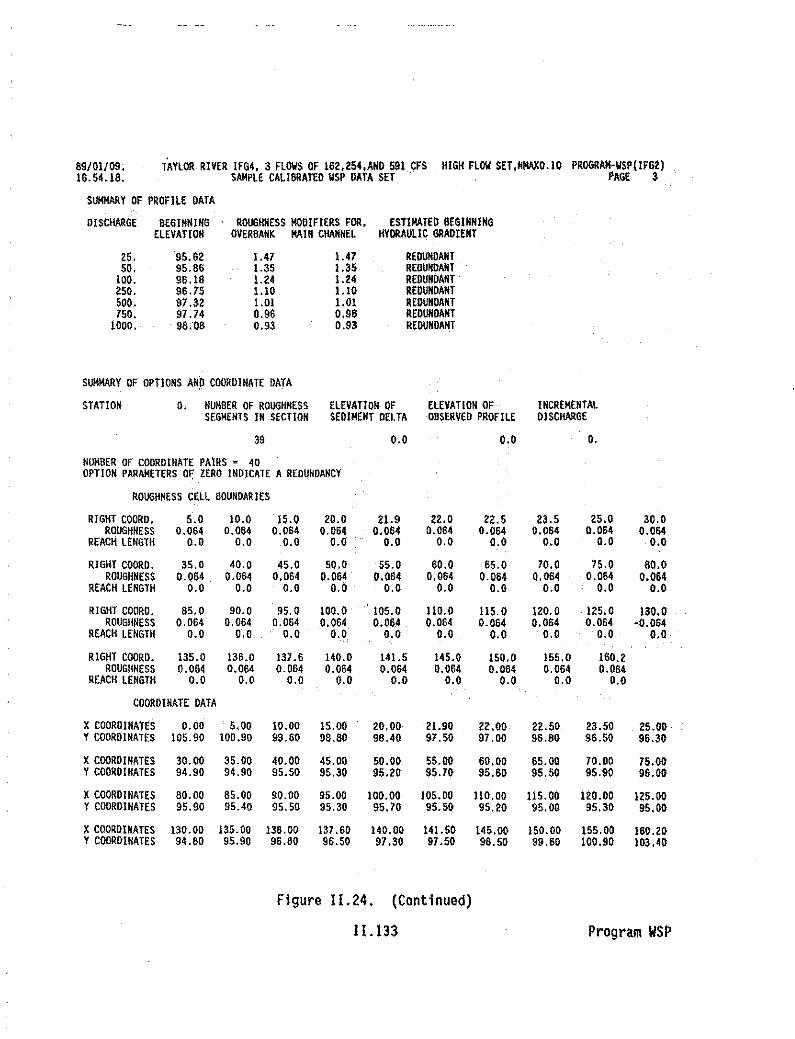
89/01/09.16.54.18.
TAYLOR RIVER IFG4. 3 FLOWS OF 162.2S4,AND 591 CFS HIGH FLOW SET,HMAXD.IO PROGRAM-WSP(IFG2)SAMPLE CALIBRATED WSP DATA SET ' ' PAGE 3
SUMMARY OF PROFILE DATA
DISCHARGE 8£GINNING ROUGHNESS MODIFIERS FOR. ESTIMATED GEGINNINGELEVATION OVER8ANK MAIN CHANNEL HYDRAULIC BRADIENT
25. '95.62 1.47 1.41 REDUNDANT50. 95.86 1.35 1.35 REOU~OAMT
100. 96.18 1.24 1.24 REDUNDAHT250. 96.75 1.10 1.](1 REDUNDANT500. 97.32 1.01 1.01 REDUNDANT750. 97.74 0.96 0.96 REDUNDANT
1000. 98.09 0.93 0.93 REDUNDANT
SUMMARY OF OPTIONS AND COORDINATE DATA
STATION O. NUH8ER OF ROUGHHESS ELEVATION OF ELEVATION OF INCREIlENTALSEGMENTS IN SECTION SEOINENT DELTA 08SERVED PROFILE DISCHARGE
39 0.0 0.0 D.
NUH8ER OF COORDINATE PAIRS • 40OPTION PARAMETERS OF ZERO INDICATE A REDUNDANCY
ROUGHNESS CELL 80UNDARIES
RIGHT COORD. 5.0 10.0 15.0 20.0 21.9 22.0 22.5 23.5 25.0 30.0ROUGHNESS 0.064 0.064 0.064 0.064 0.064 0.064 0.064 0.064 0.064 0.064
REACH LENGTH 0.0 0.0 0.0 0.0 0.0 0.0 0.0 0.0 0.0 0.0
RIGHT COORD. 35.0 40.0 45.0 50.0 55.0 60.0 65.0 70.0 75.0 80.0ROUGHNESS 0.064 0.064 0.064 0.064 0.064 0.064 0.064 0.064 0.064 0.064
REACH LENGTH 0.0 0.0 0.0 0.0 ' 0.0 0.0 0.0 0.0 0.0 0.0
RIGHT COORD. 85.0 90.0 95.0 100.0 105.0 110.0 m.o 120.0 125.0 130.0ROUGHNESS 0.064 0.064 0.064 0.064 0.064 0.064 0.064 0.064 0.064 -0.064
REACH LENGTH 0.0 0.0 0.0 0.0 0.0 0.0 0.0 0.0 0.0 0.0
RIGHT COORD. 135.0 136.0 137.6 140.0 141.5 145.0 150.0 155.0 160.2ROUGHNESS 0.064 0.064 0.064 0.064 0.064 0.064 0.064 0.064 0.064
REACH LENGTH 0.0 0.0 0.0 0.0 0.0 0.0 0.0 0.0 0.0
COORDINATE DATA
XCOORDINArES 0.00 S.OO 10.00 15.00 20.00 21.90 22.00 22.50 23.50 25.00YCOORDINATES 105.90 100.90 99.60 98.80 98.40 97.50 97.00 96.80 96.50 96.30
XCOORDINATES 30.00 35.00 40.00 45.00 50.00 55.00 60.00 65.00 70.00 75.00YCOORDINATES 94.90 94.90 95.50 95.30 95.20 95.70 95.60 95.50 95.90 96.00
XCOORDINATES 80.00 85.00 90.00 95.00 100.00 105.00 110.00 115.00 120.00 125.00YCooRDlHATES 95.90 95.40 95.50 95.30 95.70 95.50 95.20 95.00 95.30 95.00
XCOORDINATES 130.00 135.00 136.00 137.60 140.00 141.50 146.00 160.00 IS5.00 160.20YCOORDINATES 94.80 95.90 96.80 96.50 97.30 97.50 98.50 99.60 100.90 103.40
Figure 11.24. (Continued)
11.133 Program WSP

89/01/09.16.54.18.
TAYLOR RIVER IFG4. 3 FLOI/S OF 162.254,ANO 591 CFS HIGH FLOII SET .NMAXO.lO PROGRAM-I/SP(IFG2)SAMPLE CALIBRATED liSP DATA SET PAGE 5
STATIOR 0 + 0 ENGLISH SYSTEM ASSUMED ELEV. 0.00 THALIlEG ELEV. 94.8 THALIlEG SLOPE O.OODO
TH[S IS A CONTROL SECT[OR -CONPUTATION L[NE NOT REQO
LENGTH OF CONVEYANCE lfIDRAUlIC ROUGHNESSCENTROID AREAS TOP 1I10THS RADII· COEFFICIENTS
CONVEYANCEFACTORS VELOCITIES DISCHARGES
NOTE: The following 20 lines of information WOULO NOT be printed if Option 10was set to "T",
0.0 0.9 2.6 0.3 0.09408 7. 0.77 I0.0 3.6 5.0 0.7 0.09408 46. 1.26 50.0 2.1 5.0 0.4 0.09408 19. 0.87 20.0 1.1 5.0 0.2 0.09408 6. 0.57 [0.0 1.9 5.0 0.4 0.09408 IS. 0.8[ 10.0 0.9 4.2 0.2 0.09408 5. 0.55 00.0 0.0 1.0 0.0 0.09409 O. 0.07 00.0 0.4 5.0 0.1 0.09408 I. 0.27 00.0 0.1 1.5 0.[ 0.09408 o' 0.24 00.0 0.2 2.2 0.1 0.09409 1. 0.36 00.0 0.9 5.0 0.2 0.09408 4. 0.48 00.0 [ .1 5.0 0.2 0.09408 6. 0.57 I0.0 0.6 4.0 0.2 0.09408 3. 0.46 00.0 0.2 3.0 0.[ 0.09408 O. 0.24 00.0 1.4 5.0 0.3 0.09408 9. 0.65 I0.0 2.6 5.0 0.5 0.09408 27. 1.0[ 30.0 2.4 5.0 0.5 0.09408 22. 0.94 20.0 2.4 5.0 0.5 0.09408 22. 0.94 20.0 3.6 . 5.0 0.7 -0.09408 46. 1.25 50.0 1.5 3.7 0.4 0.09408 13. 0.85 I
SUM OR AVG 28. 82. 0.4 0.09408 253. 1.01 25
THIS 5ECTION HAS 39 ROUGHNESS SEGMENT(S). 20 SEGHfHT(S) IIERE USED FOR THiS OISCHARGE.THIS SECTION IS AN INITIAL CONTROL - FLOW IS SU8-CRITlCAl - CONPUTED SLOPE· 0.00979 11.5. ELEV•• 95.62
SECTIONS OF SAMPLE OUTPUT HAVE BEEN DELETED HERE FOR BREVITY.
NOTE: This type of output is generated for each flow for each cross section.
ENDR
Figure 11.24. (Concluded)
11.134 Program WSP

Ill. IrISP ERROR MESSAGES
Refer to Appendix A for "IrISP Data Set File Format".
1. NO PARD LINE FOUND IN WSP DATA SET.Either the PARD line is missing or only one title line was used and thePARD line was read as the second title line.
2. INVALID TYPE •• NOT METERS OR BlANK.Field on the PARD line indicating units of measurement used was somethingother than Blank for English or METERS for Metric.
3. CRITICAL DISCHARGE CONSTANT INVALID.Field on the PARD line indicating critical discharge constant containssomething other than "0" or "1".
4. MAXIMUM OF ... DISCHARGES EXCEEDED.There are more QARD lines than indicated on the PARD line.
5. NO DISCHARGES SPECIFIED.Either there are noQARD lines or the f1eld.on the PARD line indicatingthe number of flows to be run was left blank.
6. NO QARD LINE FOUND IN WSP DATA SET.Either there are no QARD lines or the field on the PARD line indicatingthe number of flows to be run is greater than the number of QARD lines.
7. EXPECTED LINE NOT RECEIVED .. CHECK DATA SET STRUCTURE.Either lines are out of order, a line is missing, or there is a blank linein the data set.
8. INVALID CHARACTER IN OPTION SELECTION.Valid option values on the Option Contol line are Fl T, or blank (blank=F).Something other than these values has been entered.
9. INVALID OPTION SPECIFIED.Option has been turned on, but the appropriate eTR line has not beensupplied for that option.
10. OPTION LINE RECEIVED FOR UNSELECTED OPTION.CTR lines have been supplied for an option, but the relatedopt10n hasnot been turned on.
11. MORE THAN THE SPECIFIED NO. OF OPTIONS " RECEIVED.Either this error or error 10 above wi".appear if eTR lines were suppliedfor an option, but the related option was not turned on.
12. NUMBER OF OPTIONS RECEIVED DOES NOT EQUAL NUMBER SPECIFIEDNUM. REC•••• NUM. SPEC••••••This error is somewhat redundant. If error 8, 9, 10, or 11 is listed,this will probably be listed also.
II .135 Program WSP

13. MAXIMUM OF ... CROSS SECTIOIIS EXCEEDED.On some eTR lines you are asked to enter the number for cross sectionsthat the option applies to. This error appears if data is not suppliedfor the number of cross sections specified, or if data is missing, or ifthe number specified is greater than 100.
14. STATIONS ARE 1I0T III ASCENDING ORDER FROM LOWEST TO HIGHEST ON INPUT LINE.The coordinate and roughness line stationing must increase from low to highon the input line. If this message appears, the cross section stationingdoes not consistently increase as you move away from the zero point.Check the Xcoordinates on both the Coordinate and Roughness lines. Thismessage may also appear if an asterisk (*) is missing from the lastRoughness line in a series.
15. MAXIMUM OF 99 SEGMENTS EXCEEDED.The program is dimensioned to handle up to 99 roughness segments per cross,section. These roughness segments are entered on the Roughness lines.
16. NO ROUGHNESS SEGMENTS PROVIDED.There are no Roughness lines in the data set; or there is not an asterisk(*) in Column 80 on a Roughness line; or there is not a minus sign on theroughness coefficient indicating the thalweg or main channel.
17. VTRAN CANNOT BE EQUAL TO ZERO.Zero is not a valid value for the elevation increment or slope forelevation transposition which was entered in Columns 71·75 on the Roughnesslines.
18. FIRST ROUGHNESS SEGMENT OUTSIDE COORDINATE BOUNDS.Usually refers to the left side coordinates on the Roughness lines. Thefirst right boundary of the first roughness segment has been entered asbeing before the first coordinate station (i.e., outside the coordinatedata set). For example, the first station on the Roughness line is at 10feet, but the first station on the Coordinate line.ls 20.
19. NO POINT TO LEFT OF FIRST POINT.Similar to #18. Usually occurs when the first roughness segment coordinateis given as zero.
20. RIGHT HAND ROUGHNESS SEGMENT ESTABLISHED AT RIGHT HAND COORDINATE POINT.The right-most roughness segment boundary is less than the right"mostcoordinate. The program adds a roughness segment to be a cell betweenthe last right-hand roughness segment and the right-most coordinate.
21. NO THALWEG VALUE PROVIDED FOR THIS CROSS SECTION.No minus sign has been entered to mark the thalweg or main channelroughness segment.
II .136 Program WSP

22. OVERBANK RULE VIOLATED.If an overbank (no minus sign) roughness segment is assigned to one sideof the main channel or thalweg, an overbank roughness segment must beassigned to the other side. Al so, if one cross section has overbankroughness segments, all other cross sections must have them as well. Thiscould al so happen if the thalweg is squeezed over to one side of thechannel and it is the first roughness segment.
23. STATION SPACING OR CRITICAL CONSTRAINT IS PROJECTED TOO FAR.This error usually occurs when there is a large elevation change betweentwo cross sections. This could imply that your stations are too far apart.However, when the elevation change is extreme, distance between stationscould be quite small and still produce thi s problem. Remedy thi s byestablishing an intermediate cross section to reduce the step change inelevation.
24. UNEXPECTED END OF FILE.The ENOJ or ENOR lines are missing from the data set, or you are tryingto run an empty input file.
25. NO COORDINATE DATA PROVIDED FOR DOWNSTREAM CROSS SECTION.No coordinate data was entered and there was not an elevation incrementor slope entered into Columns 71-75 on a Roughness line.
26. ZERO-ENERGY BALANCE VOIDED M.S. ELEY. ---This is a warning that the slope of the stream is so small that it isalmost level. The program cannot detect an energy loss. Since it cannotbe negative, that would indicate water was running uphill, the programset the value to "0".
27. WARNING - ONLY ONE CROSS SECTION IN THIS DATA SET.Since WSP uses the step-backwater method to predict water surfaceelevations, it uses the water surface elevations at the first crosssection, which are given. Therefore, if only one cross section is in thedata set, no water surface elevations are being predicted.
I I.l37 Program WSP

IfSPTOHC ProgramI. INTRODUCTION
The WSPTOHC program converts a WSP data set to an HEC2 input file.
The HEC2 program is not part of PHABSIM. but it can be used to determinewater surface elevations. The HEC2 program uses step backwater calculations todetermine water surface elevations.
The HEC2 program was developed, and is supported, by the HydrologicEngineering Center of the U.S. Army Corps of Engineers. Refer to the "HEC-2Water Surface Profile Users Manual" for program dOCumentation.
II. RUNNING WSPTOHC
RWSPTHC,ZWSP,ZHEC2
ZWSP=WSP data set (input)ZHEC2=HEC2 input file (output)
Figure 11.25 contains an HEC2 input file resulting from running WSPTOHCon the Sample WSP Data Set in Appendix A.
TITAYLOR RIVER IFG4. 3 FLOW> OF 162,254,ANO 591 CFS HIGH FLOW SET,NMAXO.IOT2SAMPLE CALIBRATED ~SP DATA SETT3 ORIGINAL DATA WAS FOR THE ~SP PROORAM 88/0./30.JI 2 0.000000 0 0.5 O. 95.6J2 1 1 0 0 0 1.4700 2.5 6 00J3 38 43 1 4 5 6 7 B 10QT 7 25. 50. 100. 250. 500. 750. 1000.NC 0.064 0.06400 0.06400 0.100000.50000Xl 0 40 125.0 130.0 0.0 0.0 0.0 0.0 00GR 105.9 0.0 100.9 5.0 99.6 10.0 98.8 .15.0 98.4 20.069 97.5 21.9 97.0 22.0 96.8 22.5 96.5 23.5 96.3 25.0GR 94.9 30.0 94.9 35.0 95.5 40.0 95.3 45.0 95.2 50.0G9 95.7 55.0 95.6 60.0 95.5 65.0 95.9 70.0 96.0 75.0G9 95.9 80.0 95.4 65.0 95.5 90.0 95.3 95.0 95.7 100.0GR 95.5 105.0 95.2 110.0 95.0 115.0 95.3 120.0 95.0 125.0G9 94.8 130.0 95.9 135.0 96.8 136.0 96.5 137.6 97.3 140.0GR 97.5 141.5 96.5 145.0. 99.6 150.0 100.9 155.0 103.4 160.2NC 0.064 0.06400 0.06400 0.10000 0.50000Xl 67 41 100.0 105.0 67.0 67.0 67.0 0.0 00GR 105.4 0.0 102.3 5.0 100.0 10.0 97.8 13.0 97.5 13.1G9 97.1 15.0 97.1 15.6 96.8 16.5 96.0 20.0 95.9 25.0GR 96.4 30.0 95.8 35.0 95.2 40.0 95.5 45.0 95.5 50.0GR 96.1 55.0 96.2 60.0 96.4 65.0 98.4 70.0 96.5 75.0OR 96.3 80.0 96.4 85.0 97.0 90.0 95.9 95.0 95.5 100.0G9 95.0 105.0 95.0 110.0 95.3 115.0 97.1 120.0 95.9 125.0GR 95.6 130.0 95.• 135.0 96.5 136.4 98.8 139.5 97.0 140.0OR 97.5 142.6 98.4 145.0 99.7 150.0 101.4 155.0 102.5 160.0G9 103.9 162.9
Figure 11.25. Sample HEe2 input file resulting from running WSPTOHC on a WSPdata set.
11.138 Program WSPTOHC

HIGH FLOW SET,HMAXO.IO
0.5 O. 96.22.5 6 00
HI6H FLOW SET,HMAXO.l0
0.5 O. 91.32.5 ,6 00
HIGH FLOW sET,NHAXU.10
0.5 O. 95.92.5 6 00
HIGH FLOW SET,HMAXO.IO
00
0011.830.055.080.0
105,0130.0140.0161.4
0.097.395.595.195.595.398.199.0
104.3
0, 98,16
10.025.050.015.0
100.0125.0136.2160.0
0.52.5
0.5 O. 97.12.5 6 00
HIGH FLOW SET,HMAXO.IO
0.5 O. 96,12.5 '6 00
HIGH FLOW SET.HMAXO.l0
65.097.995.096.095.595.996.19B.l
103.5
65.09.1
20.045.010.095.0
120.0135.0155.0
NC 0.064 0.06400 0.06400 0.10000 0;50DOOKl 132 40 15.0 20.0 65.0GR 105.2 0.0 101.5 5.0 96.1DR 97.0 13.5 95.3 15.0 94.7DR 95.3 35.0 95.7 40.0 95.6DR 95.9 60.0 95.7 65.0 96.1DR 95.5 85.0 95.6 90.0 98.1DR 95.0 110.0 94.7 115.0 95.0G~ 97.2 131.9 97.3 133.4 97.6GR 99.7 145.0 100.5 150.0 101.0EJ 'TITAYLOR RIVER 1~G4, 3 FLOWS OF 16Z, 254,AHO 591 CFSTZSAMPLE CALIBRATED WSP OATA SETT3 ORIGINAL DATA WAS FOR THE WSP PROGRAM 88/06/30.JI, 3 0·000000 0J2 ZOO 0 0 1.3SDGTITAYLOR RIVER IFG4, '3 FLOWS OF 162,254,AH0591 CF5T2SAHPLE CAllGRATEO WSP OATA SETT3 ORIGINAL OATA WAS FOR THE WSP PROGRAM 88/06/30.JI 4 0.000000 0JZ 3 0 0 0 . a 1.2400TITAVLOR RIVER IFG4, 3 FLOWS OF 162.254,AHO 591 CFSTZSAHPlE CALIBRATED WSP OATA SETT3 ORIGINAL DATA WAS FOR THE WSP PROGRAM 88/06/30.JI 5 . ,- 0.000000 0J2 4 0 0 0 0 1.1000T1TAYLOR RIVER IFG4, 3 FLOWS OF 16Z.254,ANO 591 CFSTZSAHPLE CAllGRATED W,SP DATA SET ,T3 ORIGINAL DATA WAS FOR THE WSP PROGRAM 8B/06/30.JI 60.0000DO 0J2 5 0 0 0 0 1.0100TITAYLOR RIVER IF84. 3 FLOWS OF 162.2S4.AHO 591 C~ST2SAMPLE CALIBRATED WSP DATA SETT30RIGINAL DATA WAS FOR THE WSP PROGRAM 8B/06/30.Jl ,7 O.DOOOOO 0J2 6 0 0 0 0 0.9600
, TlTAYLOR RIVER IFG4.3 FLOWS OF 16Z,254,ANO 591 CFST2SAMPLE CAll6RATEO WSP DATA SETT3 ORIGINAL OATA WAS FOR THEWSP PROGRAM 88/0B/30.JI 80.000DOO 0J2 IS 0 0 0 0 -0.9300
ER
Figure 11.25. (Concluded)
II .139 Program WSPTOHC
III. CROSS SECTION AND HYDRAULIC PROPERTIES FILE PROGRAMS(TAPE3 AND TAPE4/TP4 OR TAPE4A/TP4A)
INTRODUCTION
The TAPE3 and TAPE4/TP4 (TAPE4A/TP4A) fll es are unformatted fi 1es generatedfrom the hydraulic simulation programs; where TAPE3 contains cross section andreach data, TAPE4 contains flow data, and TP4 is a rearranged TAPE4 in a formatacceptable by the habitat simulation programs.
TP4 can be used in place of TAPE4 ifi any of the programs in this group.Also TAPE4A can be used in place of TAPE4, and TP4A can be used in place of TP4.TAPE4A and TP4A contain the cell velocities calculated at the verticals whenIOC(l7)~l in the IFG4 program, 1OC(11)=2 in the MANSQ program, 01' Option 1. isselected in the DIRI4 program. TAPE4A and TP4A·are used as input to the HABTAMor HABTAV habitat simulation programs.
When the cell velocities are calculated at the v~rticals to be used withHABTAM or HABTAV, the TAPE4 and TP4 resulting from the hydraulic simulationprogram must be renamed to TAPE4A and TP4A by the user, orTAPE4A and TP4A shouldbe substituted in place of the default output filenames forTAPE4 and TP4.
The programs presented in thiS chapter allow the user to list, modify,extract, or combine information from various TAPE3 or TAPE4/T?4files. Programsare also available to convert the files from unformatted to formatted files andvice versa to allow them to be transferred from computer to computer.
,.The selection of partial data from the TAPE3 or TAPE4/TP4 files may be
desired in some instream flow. studies to analyze the physical habitat versusstreamflow relationship for an individual cross section or for a series of crosssections less than the total series for a study reach. Also, detailed analysissometimes needs to be done for one streamflow but not for all of the flowssimulated in the hydraulic simulation program.
111.1

~ISTING INFORMATION fROM TAPE3 AND IAPE4(TP4) FILES
PROGRAM BATCH/PROCEDURENAME FILENAME· FUNCTION PROGRAM DESCRIPTION
lSTTP3 RLSTTP3 TAPE3 lists the contents of a TAPE3 file.listing
lSTTP4
lSTP34
CMPWSL
RlSTTP4
RlSTP34.
RCMPWSl
TAPE4Listing
TAPE3/4listing
TAPE4listing
IlL?
RlSTTP3,ZOUT,TAPE3
ZOUT=lSTTP3 results (output)TAPE3~unformatted cross section andreach data (input)
lists the contents of a TAPE4 file.
RLSTTP4,ZOUT,TAPE4
ZOUT~LSTTP4 results (output)TAPE4~unformatted flow data (input)
lists the contents of a TAPE3 and TAPE4file.
RlSTP34,ZOUT,TAPE3,TAPE4
ZOUT~LSTP34 results (output)TAPE3=unformatted cross section andreach data (input)
TAPE4=unformatted flow data (input)
Compares the water surface eIevat ionsin two TAPE4 files.
RCMPWSl,TAPE4A,TAPE4B,ZOUT,TAPE3
TAPE4A=TAPE4 file (input)TAPE4B=TAPE4 file (input)ZOUT=WSl comparison listing of the
two TAPE4's (output)TAPE3=title lines read from the TAPE3,if supplied. If not supplied, useris prompted to enter two title 1ines(input)
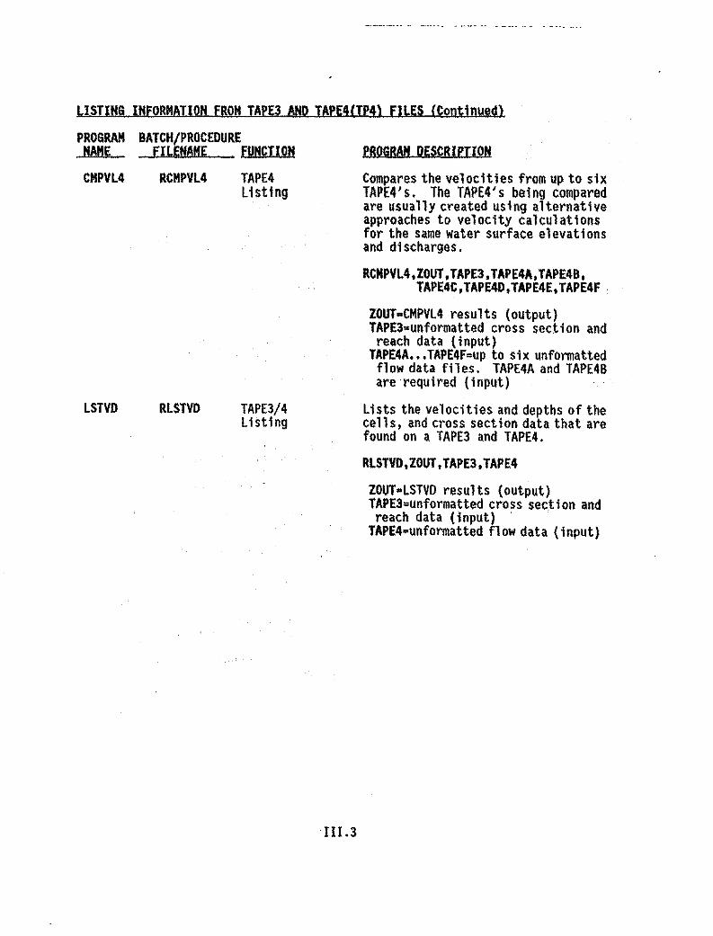
LISTING INFORMATION FROM TAPE3 AND TAPE4(TP4) FILES (Continued)
PROGRAM BATCH/PROCEDURENAME fILENAME FUNCTION
CMPVL4 RCMPVL4 TAPE4Listing
PROGRAM DEscRIPIION
Compares the velocities from up to sixTAPE4's. The TAPE4's being comparedare usually created using alternativeapproaches to velocity calculationsfor the same water surface elevationsand discharges.
LSTVD RLSTVO TAPE3/4listing
Ill.3
RCMPYL4,ZOUT,TAPE3,TAPE4A,TAPE4B,TAPE4C,TAPE40,TAPE4E,TAPE4F
ZOUT=CMPVL4 results (output)TAPE3=unformatted cross section andreach data (input)
TAPE4A•••TAPE4F=up to six unformattedflow data files. TAPE4A and TAPE48are·required (input)
lists the velocities and depths of thecells, and cross section data that arefound on a TAPE3 and TAPE4.
RLSTYD,ZOUT,TAPE3,TAPE4
ZOUT-LSTVD results (output)TAPE3=unformatted cross section andreach data (input)
TAPE4=unformatted flow data (input)
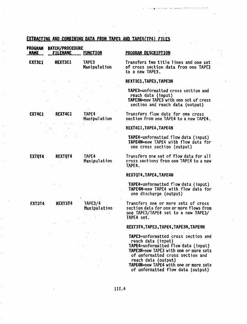
PROGRAM DESCRIPTION
Transfers two title lines and one setof cross section data from one TAPE3to a new TAPE3.
."._ .. - .•. _..__..- '--'." ..... '
EXTRAtIING AND COHBIHIHG'DATA FROM TAm AND TAPE4(TP4) fILES
PROGRAM BATCH/PROCEDURENAME FILENAME FUNCTION
EXT3CI REXT3CI TAPE3Manipulation
REXT3Cl,TAPE3,TAPE3N
EXT4Cl
EXTQT4
o.T3T4
REXT4Cl
REXTQT4
REXT3T4
TAPE4Manipulation
TAPE4Manipulation
TAPE3/4Manipulation
TAPE3-unformatted cross section andreach data (input)
TAPE3N-new TAPE3 with one set of crosssection and reach data (output)
Transfers flow data for one crosssection from one TAPE4 to a new TAPE4.
REXT4Cl,TAPE4,TAPE4H
TAPE4-unformatted flow data (input)TAPE4N-new TAPE4 with flow data for
one cross section (output)
Transfers one set of flow data for a11cross sect ions from one TAPE4 to a newTAPE4.
REXTQT4,TAPE4,TAPE4H
TAPE4-unformatted flow data (input)TAPE4H-new TAPE4 with flow data forone discharge (output)
Transfers one or more sets of crosssect ion data for one or more fl ows fromone TAPE3/TAPE4 set to a new TAPE3/TAPE4 set.
REXT3T4,TAPE3,TAPE4,TAPE3H,TAPE4H
TAPE3-unformatted cross section andreach data (input)
TAPE4-unformatted flow data (input)TAPE3H-new TAPE3 with one or more setsof unformatted cross section andreach data (output)
TAPE4N-new TAPE4 with one or more setsof unformatted flow data (output)
I1I.4

PROGRAM DESCRIPTION
Combines two TAPE3 files.
RCOMTP3,TAPE3A,TAPE3B,TAPE3N
EXTRACTING AND COMBINING DATA FROM TAPE3 AND TAPE4(TP4) FILES (Continued)
PROGRAM BATCH/PROCEDURENAME FILENAME FUNCTION
COMTP3 RCOMTP3 TAPE3Manipulation
COMTP4 RCOMTP4 TAPE4Manipulation
TAPE3A-unformatted cross sect ion andreach data (input)
TAPE3B=unformatted cross section andreach data (input)
TAPE3N-combined TAPE3 files (output)
Combines two TAPE4 files. User canselect option to specify a divisionflow where flows less than or equalto the division flow are transferredfrom the first TAPE4 and combinedwith flows greater than the divisionflow from the second TAPE4.
RCOMTP4,TAPE4A,TAPE4B,TAPE4N
TAPE4A-unformatted flow data (input)TAPE4B=unformatted flow data (input)TAPE4N-combined TAPE4 files loutput)
MODIFYING IAPE3 AND TAPE4{TP4) FILES
ADDBEND RADBEND TAPE3Modification
Adds left and right bend weights toa TAPE3.
RADBEND,TAPE3,TAPE3N
TAPE3-unformatted cross section andreach data (input)
TAPE3N-modified TAPE3 with left andright bend weights added (output)
MODRUl RMODRLW TAPE3Modification
II 1.5
Changes cross sect ion weights and reachlengths on a TAPE3 file.
RMODRLW,TAPE3,TAPE3N
TAPE3-unformatted cross section andreach data (input)
TAPE3N-modified TAPE3 file (output)
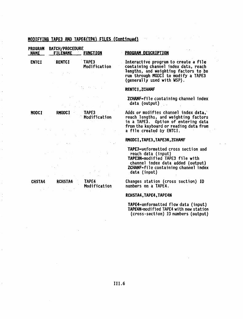
MODIFYINQ TAPE3 AND TAPE4{!P4) FILES {Continued}
PROGRAM BATCH/PROCEDURENAME FILENAME fUNCTION PROGRAM DESCRIPTION
ENTeI RENTCI TAPE3 Interactive program to create a fileModifi cati on containing channel index data, reach
lengths, and weighting factors to berun through MODel to modify a TAPE3(generally used with WSP).
RENTCI.lCHANF
lCHANF=flle containing channel indexdata (output)
HODCI RHODCJ TAPE3 Adds or modifies channel index data,·Modification reach lengths, and weighting factors
in a TAPE3. Option of entering datafrom the keyboard or reading data froma file created by ENTCI.
RMODCJ,TAPE3.TAPE3N,lCHANF
TAPE3=unformatted cross section andreach data (input)
TAPE3N=modified TAPE3 file withchannel Index data added (output)
lCHANF=file containing channel indexdata (i nput)
CHSTA4 RCHSTM TAPE4 Changes station (cross section) IDModification numbers on a TAPE4.
RCHSTA4,TAPE4.TAPE4H
TAPE4=unformatted flow data (input)TAPE4N=lIlOdified TAPE4 wi th new station
(cross-section) ID numbers (output)
III.6

CONVERTING TArE3 AND IAPE4(IP4) FILU
PROGRAM BA~~'::~EDURENAME FUNCTION
UIP34F RUIP34F TAPE3/4Conversion
PROGRAM DESCRIPTION
Converts an unformatted TAPE3 or TAPE4to a formatted TAPE3F or TAPE4F.
RUTP34F.TAPE3.TAPE3F.TAPE4,TAPE4F
(if only a TAPE4 is to be converted,use: RUTP34F,TAPE4,TAPE4F)
FTP34U IlFTP34U TAPE3/4Conversion
III.7
TAPE3~unformattedcross section andreach data (input)
TAPE3F=formatted cross section andreach data (output)
TAPE4=unformatted flow data (input)TAPE4F=formatted flow data (output)
Converts a formatted TAPE3r or TAPE4Fto an unformatted TAPE3 or TAPE4.
RFTP34U.TAPE3F,TAPE3.TAPE4F,TAPE4
(if only a TAPE4 is to be converted,use: RFTP34U,TAPE4F,TAP(4)
TAPE3F=formatted cross section andreach data (input)
TAPE3=unformatted cross section andreach data (output)
TAPE4F=formatted flow data (input)TAPE4=unformatted flow data (output)
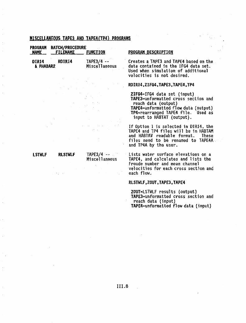
PROGRAM DESCRIPTION
MISCELLANEQYS TAP£3 AND TAP£4CTP4) PROGRAMS
PROGRAM BATCH/PROCEDURENAME FILENAME FUNCTION
DIRI4 RDIRI4! PHABAR2
TAPE3j4 --Hi see11 aneous
Creates a TAPE3 and TAPE4 based on thedata contained In the IFG4 data set.Used when simulation of additionalvelocities is not desired.
RDIRI4,ZIFG4,TAPE3.TAPE4.TP4
ZIFG4=IFG4 data set (input)TAPE3=unformatted cross section andreach data (output)
TAPE4=unformatted flow data (output)TP4=rearranged TAPE4 file. Used as
Input to f1ABTAT (output).
If Option 1 is selected in OIRI4, theTAPE4 and TP4 files will be in HABTAMand f1ABTAV readable format. Thesefiles need to be renamed to TAPE4Aand TP4A by the User.
LSTWLF RLSTWLF TAPE3!4 --Mi see11 aneous
IlLS
Lists water surface elevations on aTAPE4, and calculates and lists theFroude number and mean channelvelocities for each cross section andeach flow.
RlSTWLF,ZOUT,TAPE3.TAPE4
ZOUT=lSTWLF results (output)TAPE3=unformatted cross section andreach data (input)
TAPE4=unformatted flow data (input)

MISCELLANEOUS TAPE3 AND TAPE4CI(4) PROGRAMS (Continued)
PROGRAM BATCH/PROCEDURENAME FILENAME FUNCTION PROGRAM DESCRIPTION
PHABAR2 RPHABARl PHABARR
PHABRTH RPHBRTH
TAPE4 -Miscellaneous
TAPE4 -Miscellaneous
Il1.9
Rearranges a .TAPE4 and writes a TP4.
RPHABAR,TAPE4,TP4.POS
IAPE4-unformatted flow data (input)IP4=rearranged TAPE4 file (output)POS. -I Leaves negative velocities
as negative numbers.(PHABARR)
POS- 1 Converts negative velocitiesto positive numbers.(PHABAR2)
(default is POS = 1) (PHABAR2)Run by the RIFG4. RWSP. and RDIRl4batch/procedure files.
Converts a TP4 file back to a TAPE4file.
RPHBRTN.TP4,TAPE4
IP4-rearranged TAPE4 file ofunformatted flow data (input)
TAPE4=unformatted flow data (output)

MDREND ProgramI. INTRODUCTION
The ADDBEND program adds left and right bend weights to a TAPE3. Thenormal use of the habitat simulation programs assumes the reach length is thesame for all cells in a cross section. This is the same as assuming the streamis straight.
The assumption of a straight stream usually does not lead to anysignificant loss in the accuracy of the calculated weighted usable area, butthere are cases where the bends are significant.
For a bend such as shown in Figure 111.1, the reach length is assumed tobe proportional to the fraction of the stream width the cell lies from thestream's edge. The cell's length can be calculated from the average reach length(RL), the multiplier for the bend on the left side (WL), and the multiplier forthe bend on the right side (WR).
If ADDBEND has been run On a TAPE3, IOC(12) must be set to "1" in thehabitat simulation programs. If IOC(12) is set to "1", and left and right bendweights have NOT been added with ADDBEND, the program will abort and the outputfile will contain a message "List Exceeds Data· Filename TAPE3".
II. RUNNING ADDBEND
RADBEND,TAPE3.TAPE3N
TAPE3~unformatted cross section and reach data (input)TAPE3N..modified TAPE3 with left and right bend weights added (output)
The follQwing prompt will be asked for each cross section on the TAPE3:
ENTER WEIGHT FOR BEND ON LEFT AND RIGHT SIDEOF CROSS SECTION ... (WL,WR):
Figure IlLl. is a diagram of how to determine left and right bend weights.
HUO . Program ADDBEND

.'"0s::
'".0'"c:0
'"+>.c:0'1.~
!jl'"0c:
'"~ .0N ....~
~ ..J 0
ce c:-j o .
*.~
0:. ce 'l;;.. s::3: .~
,.) e...'7 '"+>
'"Q
....•................
'"...:;,0'1.~
u..
III.ll Program ADDBEND

CHSTA4 ProgramI. INTRODUCTION
The CHSTA4. program changes station (cross section) ID numbers on a TAPE4.It Is most often used when an IFG4 data set using consecutive 10 numbering Isconverted to a WSP data set using stationing as cross section 10 numbering. IfWSP Is run on the WSP data set and the water surface elevations written to theTAPE4 are to be read back Into the IFG4 data set using WSEI4, the cross section10 numbering will be different on the TAPE4 than In. the IFG4 data set.Therefore, CHSTA4 must be run to change the cross section ID numbering to matchthe IFG4 data set.
II. RUNNING CHSTA4
RCHSTA4,TAPE4.TAPE4N
TAPE4~unformatted flow data (input)TAPE4N;modified TAPE4 with new station (cross section) 10 numbers (output)
STATION; •.. ENTER NEW STATION 10:
This prompt will appear for each cross section on the TAPE4.
NUMBER OF FLOWS SIMULATED· ...
111.12 Program CHSTA4

CMPVL4 Program
I. INTRODUCTION
The CMPVL4 program compares the velocities from up to six TAPE4's (TP4's,TAPE4A's, or TP4A's) •. The TAPE4's being compared are usually created usingalternative approaches to velocity cillculations for the same water surfaceelevations and discharges.
For example, you may wish to compare the velocities·calculated by runningIFG4 using one velocity set vs. using no velocity sets; or compare the resultsof the velocities calculated by IFG4 vs. MANSQ, etc. .
II. RUNNING CMPVL4
RCMPVL4.Z0UT.TAPE3,TAPE4A,TAPE48,TAPE4C,TAPE4D,TAPE4E,TAPE4F
ZOUTsCMPVL4 results (output)TAPE3-unformatted cross section and reach data (input)TAPE4A•••TAPE4F-up to six unformatted flow data files.
TAPE4A and TAPE4B are reqUired (input)
The two title lines from the TAPE3 used as input will be listed.
ENTER 1 TO LIST ONE SET OF VELOCITIES TO SCREENo TO LIST ALL VELOCITIES TO AN ALTERNATIVE FILE
If "1" js selected, the follOWing prompts appear and. the informationwill appear on the screen; no output file is created.
DISCHARGES FOUND ON FIRST TAPE4 ARE
Discharges will be listed here
ENTER THE DISCHARGE YOU WANT TO LIST:
ENTER LABELS FOR EACH FLOW DATA SET, MAX 10 CHARS - (ONE LABEL PER LINE)
Figure 111.2 contains sample output from the CMPVL4 program.
III.l3 Program CMPVL4

88/09/06. UPPER SALMON RIVER. NEAR STANLEY. PROGRAM - CHPVL409.07,46. IF64 DATA SET WITH WSL LINES ADDED FROM MANSQ AND ZERO VELOCITY SETS PAGE - 2
SECTION - 0.00 DISCHARGE - 8.00 WATER. SURFACE ELEVATiON· 97.880
VELOCITIES
oVEL Sots 1 VEL Sot
L 0.88 0.462 1.17 0.623 0.30 0.164 0.30 0.165 0.30 0.166 0.52 0.827 I.Z3 1.518 1,57 1.599 1.88 1.78
10 1.$8 2.22II 1.39 1.9012 1.23 1.4013 0.70 0.8814 0.30 0.4215 0.61 0.5416 0.30 0.12
ONLY THE COMPARISON FOR THE FIRST CROSS SECTION AND THE FIRST FLOW ARE INCLUDEDIN THIS SAMPLE OUTPUT.
Figure 111.2 Sample output from the CMPVl4 program.
III.I4 Program CMPVl4

CMPWSL Program
I. INTRODUCTION
The CMPWSl program compares the water surface elevations in two TAPE('s(TP4's, TAPE4A's, or TP4A's). The cross section 10 number, discharge, watersurface elevation from the first TAPE4, water surface elevation from the secondTAPE4, and the difference between the two are written to the output file.
II. RUNNING CMPWSL
RCHPWSL.TAPE4A.TAPE4B,ZOUT.TAPE3
TAPE4A=TAPE4 file (input)TAPE4B=TAPE4 file (input)ZOUT=WSL comparison listing of the twoTAPE4's (output)TAPE3=title lines read from the TAPE3, if supplied.If not supplied, user is prompted to enter two title lines(optional, input)
ENTER TITLE FOR THE FIRST SET (60 CHAR MAX):
ENTER TITLE FOR THE SECOND SET (60 CHAR MAX):
The output in Figure 111.3 is a comparison of the results of running IFG4and MANSQ on the same data.
II 1.15 Program CMPWSl

DATE - 88/06/16. TIME - 15.35.15. PROGRAM - CHPlI5L PAGE - 1
UPPCR SALMON RIVER. NEAR STANLEY. IDAHOCROSS SECTIONS 0 AND 14.3
FIRST SET - PREDICTED VSL'S FROM IFG4
SECOND SET - PREDICTED WSL'S FROM MANSO
CiS ID DISCHARGE FIRST SET SECOND SET DIFFERENCE
0.00 8.00 97.65 97.611 -0.020.00 10.00 97.70 97.72 -0.020.00 20.00 97.65 97.64 0.010.00 30.00 97.96 97.93 0.020.00 40.00 98.05 98.01 0.040.00 50.00 96.12 98.06 0.040.00 60.00 98.19 98.13 0.050.00 70.00 98.25 98.19 0.060.00 80.00 98.30 98.23 0.070.00 90.00 98.35 98.28 0.070.00 100.00 98.40 98.32 0.080.00 1l0.00 98.44 98.36 0.080.00 120.00 98.49 98.40 0.1190.00 130.00 98.53 98.44 0.09
14.30 8.00 98.04 98.04 0.0114.30 10.00 98.08 98·06 0.01IUD 20.00 98.22 98.22 0.0014.30 30.00 98.32 98.32 0.0014.30 40.00 98.40 98.40 0.0014.30 50.00 98.47 96.47 0.0014.30 60.00 98.53 98.53 0.00lUO 70.00 98.56 98.56 0.0114.30 60.00 98.63 98.62 0.0114.30 90.00 98.68 96.66 0.0214.30 100.00 98.72 98.70 0.0214.30 1l0.00 98.76 98.73 0.0314.30 120.00 98.80 98.77 0.0314.30 130.00 98.83 98.80 0.04
NORMAL END OF JOB
Figure 1[1.3 Sample output from the CMPWSL program.
HI.lG Program CMPWSL

COMTP3 Program
I. INTRODUCTION
The COMTP3 program combines two TAPE3 files.
II. RUNNING COMTP3
RCOMTP3,TAPE3A,TAPE3B,TAPE3N
TAPE3A=unformatted cross sect jon and reach data (input)TAPE3B=unformatted cross section and reach data (input)TAPE3N=combined TAPE3's (output)
The title lines from the two TAPE3 files will be listed.)
ENTER TWO LINE TITLE FOR NEW TAPE3N:
THE REACH LENGTH FOR THE FIRST CROSS SECTIONON THE SECOND TAPE3 FILE IS:ENTER A NEW REACH LENGTH OR ·1 TO LEAVE AS IS:
The COMTP3 program adds the second TAPE3 onto the end of the first TAPE3.Most often, the reach length on the first cross section on a TAPE3 is zero.This is not the desired reach length.when it becomes a mid-section. Thisprompt allows tile user to change the reach length on the first crosssection of the second TAPE3 file when two TAPE3 files are being combined.
III. 17 Program COMTP3

COMTP4 Program1. INTRODUCTION
The COMTP4 program combines two TAPE4 files. User can select option tospecify a division flow where flows less than or' equal to the division flow aretransferred from the first TAPE4 and combined with flows greater than thedivision flow from the second TAPE4.
II. RUNNING COMTP4
RCOMTP4,TAPE4A,TAPE4B,TAPE4H
TAPE4A=unformatted flow data (input)TAPE4B=unformatted flow data (input)TAPE4N=combined TAPE4's (output)
ENTER:o TO COMBINE TWO TAPE4'S
ADDING SECOND FILE AfTER END Of FIRST1 : TO MERGE TWO TAPE4'S, SORTING BY FLOW2 : TO MERGE TWO TAPE4'S, USING SPECIFIED
DIVISION FLOWCHOICE:
If Option ? js selected,
ENTER fLOW DIVIDING FIRST SET fROM SECOND:
flows less than or equal to the division flow are transferred fromthe first TAPE4 and combined With flows greater than the divisionflow from the second TAPE4.
HUB Program COMTP4

DIRI4 Program
1. INTRODUCTION
The DIRI4 program creates a TAPE3 and TAPE4 based on the data containedin the IFG4 data set. It is used when simulation of additional velocities isnot desired.
II. RUNNING DIRI4
RDIRI4,ZIFG4.TAPE3,TAPE4.TP4
ZIFG4-IFG4 data set (input)TAPE3-unformatted cross section and reach data (output)TAPE4-unformatted flow data (output)TP4-rearranged TAPE4 file. Used as input to HABTAT (output).
NOTE I If Option 1 is selected in DIRI4, the TAPE4 and TP4 files will be in HABTAMand HABTAV readable format. These files need to be renamed to TAPE4A andTP4A by the user.
ENTER 0 IF FLOW PROPERTIES FILE (TAPE4)IS FOR HABTAT
1 IF FOR HABTAV OR HABTAM
111.19 Program DIRl4

ENTcr Program
I, INTRODUCTION
The ENTCI program is an Interactive program to create a file containingchannel index data. reach lengths, and weighting factors to be run through MODCIto modify a TAPE3. This program is generally run when the TAPE3 resulting froma WSP run is to be used as input to the habitat simulation programs. Channelindex values are not included in a WSP data set; (channel index values of "onare written to the TAPE3 by WSP) thus they are not passed onto the TAPE3.Channel index values are used In the calculation of Weighted Usable Area (WUA)in habitat simulation.
II. RUNNING ENTCI
RENTCI,ZCHAHF
ZCHANF~file containing channel index data (output)
WHAT IS THE TITLE FOR THIS FILE (MAX 80 CHAR)-
WHAT IS THE CROSS SECTION 10 NUMBER-
WHAT IS THE REACH LENGTH-(FOR NO CHANGE IN THE REACH LENGTH ON THE CROSS SECTION ENTER -I)
WHAT IS THE WEIGHT ON THE CROSS SECTION-(FOR NO CHANGE IN THE WEIGHT ON THE CROSS SECTION ENTER -I)
HOW MANY CHANNEL INDEX VALUES ARE TO BE ENTERED FOR THIS CROSS SECTION(FOR NO CHANGE IN THE CHANNEL INDEX VALUES ON THE CROSS SECTION ENTER A 0)
If channel index values are being entered, the user will be prompted toenter the channel index values.
The above series of prompts will appear for each cross section data to bemodified. The resulting file will be used as input to MODel to add or modifythe channel index values. reach lengths, and weights on a TAPE3.
Sample ZCHANF file.
CHANNEL INDEX DATA TO BE ADDED TO ATAPE3XS£C 0.0 -I.OO-LO 3DNS 0.0 3.00 3.00 3.00NS 0.0 6.00 B.25 8.25NS 0.0 9.00 9.00 9.00HS 0.0 9.00 9.25 9.25NS 0.00 10.00 JO.OO 10.00
3.00 9.25 6.008.25· 8.25 9.009.00 9.00 9.009.25 9.25 10.008.25 3.00 3.00
III. 20 Program ENTCI

EXT3Cl Program
I. INTRODUCTION
The EXT3CI program transfers two title lines and one set of cross sectiondata from one TAPE3 to a new TAPE3.
The selection of partial data from a TAPE3 file may be desired in someinstream flow studies to analyze the physical habitat versus streamflowrelationship for an individual cross section or for a series of cross sectionsless than the total series for a study reach.
II. RUNNING EXT3CI
REXT3Cl.TAPE3.TAPE3N
TAPE3~unformatted cross section and reach data (input)TAPE3N~new TAPE3 with one set of cross section and reach data (output)
CROSS SECTION 10 NUMBERS ARE -
ENTER CROSS SECTION 10 NUMBER OF SECTION TO BE TRANSFERRED:
III. 21 Program EXT3el

EXT3T4 Program
I. INTRODUCTION
The EXT3T4 program transfers one or more sets of cross section data forone or more flows from one TAPE3/TAPE4 set to a new TAPE3/TAPE4 set.
The selection of partial data from a TAPE3 and TAPE4 file may be desiredin some instream flow studies to analyze the physical habitat versus streamflowrelationship for an individual cross section or for a series of cross sectionsless than the total series for a study reach; or for certain flows rather thanfor all the flows simulated.
II. RUNNING EXT3T4
REXT3T4,TAPE3.TAPE4.TAPE3N.TAPE4N
TAPE3~uhformatted cross section and reach data (input)TAPE4=unformatted flow data (input)TAPE3N=new TAPE3 with one or more sets of unformatted cross section
and reach data (output)TAPE4H=new TAPE4 with one or more sets of unformatted flow data (output)
DATA SET TITLE IS -
The two title lines from the TAPE3 will be displayed.
ENTER ITO CHANGE SECOND LINE OF TITLE, 0 OTHERWISE:
If "1" is selected:
ENTER NEW SECOND LINE
CROSS SECTION 10 NUMBERS ARE -
Cross section TO numbers will be listed here.
HOW MANY SECTIONS ARE TO BE TRANSFERRED?
ENTER THE _. CROSS SECTION ID NUMBER(S) TO BE TRANSFERRED:
DISCHARGES FOUND ON TAPE4 ARE -
Discharges will be listed here.
HOW MANY DISCHARGES ARE TO BE TRANSFERRED?(ENTER 0 TO TRANSFER All DISCHARGES):
ENTER OISCHARGE(S) TO BE TRANSFERRED:
111.22 Program EXT3T4

EXT4Cl Program
I. INTRODUCTION
The EXT4Cl program transfers flow data for one cross section from one TAPE4to a new TAPE4. .
The selection of partial data from a TAPE4 file may be desired in someinstream flow studies to analyze the physical habitat versUs streamflowrelationship for an individual cross section or for a series of cross sectionsless than the total series for a study reach.
II. RUNNING EXT4Cl
REXT4Cl,TAPE4.TAPE4N
TAPE4=unformatted flow data (input)TAPE4N=new TAPE4 with flow data for one cross section (output)
CROSS SECTION 10 NUMBERS ON FLOW FILE ARE·
ENTER CROSS SECTION ID OF SECTION TO BE TRANSFERRED:
Discharge information on the new TAPE4 will Include the water surfaceelevation and velocities for all flows on the TAPE4 for the cross sectionspecified.
III.23 Program EXT4Cl

EXTQT4 Program
I. INTRODUCTION
The EXTQT4 program transfers one set of flow data for all cross sectionsfrom One TAPE4 to a new TAPE4.
The select Ion of partial data from a TAPE4 file may be desired in someinstream flow studies to analyze the physical habitat versus streamflowrelationship for one flow rather than for all the flows simulated for a studyreach.
II. RUNNING EXTQT4
REXTQT4,TAPE4,TAPE4H
TAPE4~unformatted flow data (input)TAPE4H=new TAPE4 with flow data for one discharge (output)
DISCHARGES FOUND ON TAPE4 ARE -
Discharges will be listed here.
ENTER DISCHARGE TO BE TRANSFERRED
Enter the discharge to be transferred to the new TAPE4. Dischargeinformation on the new TAPE4 will include the water surface elevation andvelocities for each cross section for the flow transferred.
III.24 Program EXTQT4

FTP34U Program
I. INTRODUCTION
The FTP34U program converts a formatted TAPE3F or TAPE4F to an unformattedTAPE3 or TAPE4.
The formatted versions of these files were created by the UTP34F program.Unformatted files are likely to be incompatible between a microcomputer and theCDC mainframe, and between different microcomputers. The formatted version ofthe files should be used when transferring from computer to computer.
II. RUNNING FTP34U
RFTP34U,TAPE3F,TAPE3,TAPE4F,TAPE4
(if only a TAPE4 is to be converted,use: RFTP34U,TAPE4F,TAPE4)
TAPE3F-formatted cross section and reach data (input)TAPE3-unformatted cross section and reach data (output)TAPE4F=formatted flow data (input)TAPE4-unformatted flow data (output)
II 1.25 Program FTP34U
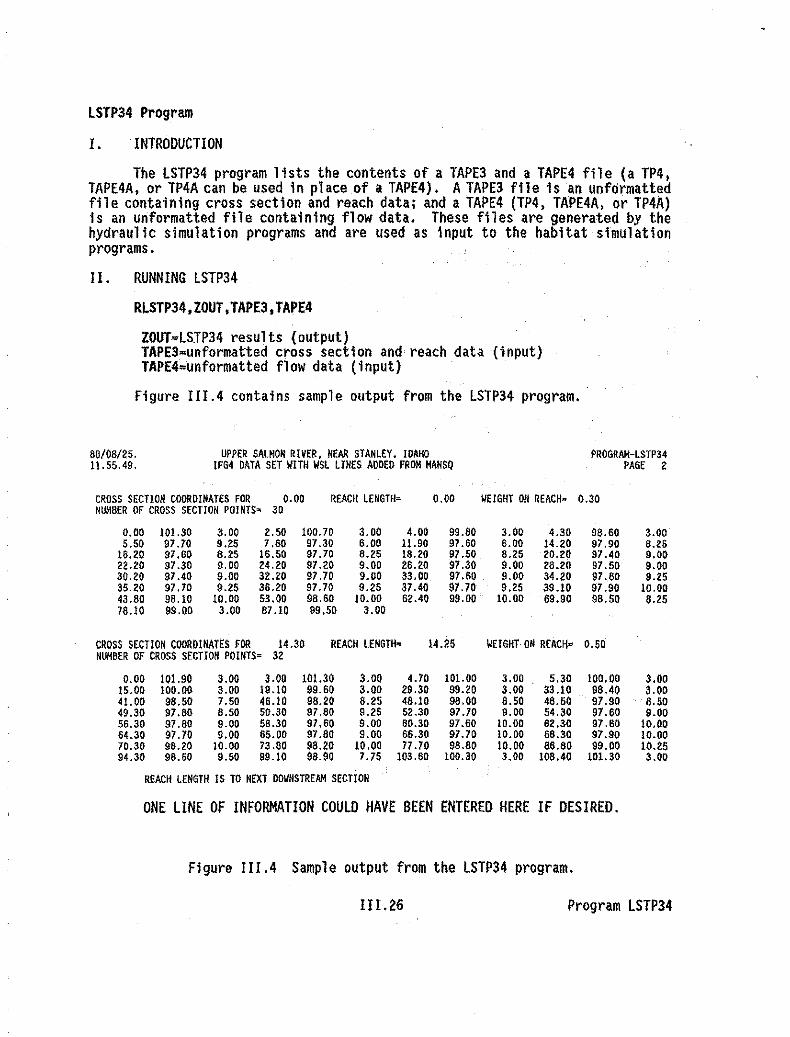
LSTP34 Program
I. INTRODUCTION
The LSTP34 program lists the contents of a TAPE3 and a TAPE4 file (a TP4,TAPE4A, or TP4A can be used in place of a TAPE4). ATAPE3 file is an unformattedfile containing cross section and reach data; and a TAPE4 (TP4, TAPE4A, or TP4A)is an unformatted file containing flow data. These files are generated by thehydraulic simulation programs and are used as input to the habitat simulationprograms.
fl. RUNNING lSTP34
RLSTP34, ZOUT,TAPE3,TAP£4
ZOUT~LSTP34 results (output)TAPE3=unformatted cross section and reach data (input)TAPE4=unformatted flow data (input)
Figure III.4 contains sample output from the LSTP34 program..
88/08125. UPPER SALMOij RIVER. nEAR STAijLEY. IDAHO PROGRAM-LSTP3411.55.49. IFG4 DATA SET WITH WSL LlijES ADDED FROM MANSQ PAGE 2
CROSS SECTION COORDINATES FOR 0.00 REACH LENGTH· 0.00 WEIGHT ON REACH· 0.30NUM8ER OF CROSS SECTION POINTS. 30
0.00 101.30 3.00 2.50 100.70 3.00 4.00 99.80 3.00 4.30 98.60 3.005.50 97.70 9.25 7.60 97.30 6.00 11.90 97.60 6.00 14.20 97.90 8.26
16.20 97.60 8.25 16.50 97.70 8.25 18.20 97.50 8.25 20.20 97.40 9.0022.20 97.30 9.00 24.20 97.20 9.00 26.20 97.30 9.00 28.20 97.50 9.0030.20 97.40 9.00 32.20 97.70 9.00 33.00 97.60 9.00 34.20 97.60 9.2535.20 97.70 9.25 36.20 97.70 9.25 37.40 97.70 9.25 39.10 97.90 10.0043.80 98.10 10.00 53.00 98.60 10.00 62.40 99.00 10.00 69.90 98.50 8.2578.10 99.00 3.00 87.10 99.50 3.00
CROSS SECTION COORDINATES fOR 14.30 REACH LENGTH· 14.25 WEIGHT ON REACH- 0.50NUHBER Of CROSS SECTION POINTS· 32
0.00 101.90 3.00 3.00 101.30 3.00 4.70 101.00 3.00 5.30 100.00 3.0015.00 100.00 3.00 19.10 99.60 3.00 29.30 99.20 3.00 33.10 98.40 3.0041.00 98.50 7.50 46.10 98.20 8.25 48.10 98.00 8.50 48.50 97.90 8.5049.30 97.60 8.50 50.30 97.80 9.25 52.30 97.70 9.00 54.30 97.60 9.0056.30 97.80 9.00 S6.30 97.60 9.00 80.30 97.60 10.00 62.30 97.60 10.0054.30 97.70 9.00 65.00 97.80 9.00 66.30 97.70 10.00 66.30 97.90 10.0070.30 96.20 10.00 73.80 98.20 10.00 n.70 96.80 10.00 86.80 99.00 10.2594.30 96.60 9.50 99.10 98.90 7.75 103.60 100.30 3.00 109.40 101.30 3.00
REACH LEijGTH IS TO NEXT OO~NSTREAM SECTion
ONE LfNE OF INFORMATION COULD HAVE BEEN ENTERED HERE IF DESIRED.
Figure III.4 Sample output from the lSTP34 program.
III. 26 Program lSTP34

88/06/25.11.5?49.
UPPER 3M-MON RIVER. HEAR STANLEY. IDAHOIfG4 DATA SET WITH WSL lINES ADDEO fROM KlHSQ
PROGRAH·LSTP34PAGE 3
Q RELATED DATA fOR THE CROSS SECTION 0.00DiSCHARGe • 8.00 KUM8ER Of VElOCITIES • IS WsL • 97.88
VELOCITIES 0.46 0.62 0.16 0.16 0.16 0.62 1.51 1.59 1.78 2,221.90 1.40 0.63 0.42 0.54 0.12
Q RELATED DATA fOR THE CROSS SECTION 0.00DISCHARGE' 10.00 NUHaER OF VElOCITIES • 20. WSL " 97.72
VElOCITIES 0.03 G.52 0.69 0.21 0.21 0.27 0.76 1.67 1.71 1.872.33 2.07 1.56 0.96 0.81 0.70 0.20 0.18 0.28 0.13
QRELATED DATA FOR THE CROSS SECTION 0.00DISCHARG\O " 20.00 NUMBER OF VELOCITIES' 20 1151" 97.84
VELOCITIES 0.14 D.78 1.00 0.37 o.a7 0.62 1.30 2.37 2.30 2.41 .3.02 2.87 2.24 2.05 2.08 1.23 0.46 0.72 1.07 0.54
QRELATED DATA fOR THE CROSS SECTION 0.00DISCHARGE " 30.00 NUMBER OF. VELOCITIES " 21 WSI " 97.93
VELOCITIES 0.21 0.95 1.22 0.5& 0.58 O.~B 1.&6 2.87 2.72 2.793.50 3.44 2.72 2.75 2.&6 1.61 0.62 l.05 1.58 0.990.20
SECTIONS OF SAMPLE OUTPUT HAVE BEEN· DE~ETED HERE FOR BREVITV.
SUMMARY OF WEIGHTS ON SECTIONS
EFFECTIVECROSS SEC REACH LENGTH WEIGHT PERCENT
0.014.3
4.289.97
O.SO 30.000.50 70.00
TOTAL LENGTH OF STUDY REACH 15 14.25
ONE LI~E OF INFORMATION COULD HAVE BEEN ENTERED HERE IF DESIRED.
NORMM- END Of JOO
Figure 111.4 (Concluded)
II 1.27 Program LSTP34

LSTIP3 ProgrMl
I. INTRODUCTION
The LSTTP3 program lists the contents of a TAPE3 file. A TAPE3 file isan unformatted file containing cross section and reach data generated by thehydraulic simulation programs and used as input to the habitat simulationprograms.
II. RUNNING LSTTP3
RLSTTP3,ZOUT,TAPE3
ZOUT-LSTTP3 results (output)TAPE3-unformatted cross section and reach data (input)
LIST TAPE3 OPTIONS:1) FULL LISTING2) PARTIAL LISTING
ENTER CHOICE:
FULL LIstING _ Cross section 10 number, reach length, weight onreach, number of cross section points, left andright reach length weights (if added with AOOBENO),and the X,V coordinate pairs with their associatedchannel index/roughness values.
PARTIAL LISTING - The X,V coodinate pairs with their associatedchannel index/roughness values are not listed asin the full listing.
Figure 111.5 contains sample output from the LSTTP3 program.
IIL2S Program LSTTP3

RESULTS WHEN A ~PARTIAL LISTING~ IS SELECTED WITH THE LSTTP3 PROGRAM
UPPER S~LMOR RIVER, RE~R ST~RLEY, 10~HO
IFG4 O~TA SET WITH WSL LINES ~OOEO FROM M~NSQ
88/08/22.16.15.27.
CROSS SECTION. 0.0 REACH LENGTH'NUMBER OF CROSS SECTION POINTS' 30
CROSS SECTION • 14.3 REACH LERGTH •NUMBER OF CROSS SECTION POINTS' 32
0.00
14.25
PROGRAM - LSTTP3PAGE - 2
WEIGHT OR REACH· 0.30
WEIGHT ON RE~CH' 0.50
FOR TOT~L RE~CH
CROSS SEC RE~CH LENGTH CIS WEIGHT LENGTH PERCENT
0.014.3
0.0014.25
0.300.50
4.2B 30.009.97 70.00
LSTTP3 RESULTS WHEN THE TAPE3 CONTAINS WEIGHTS FOR BENDS WHICH WERE ADDEDUSING THE ADDBEND PROGRAM
88/08/22.16.18.17.
SALHON RIVER, NEW YORK. UNSTEADY FLOW MODEL, SUMMER 1986 (CPINM)PINEVILLE SI16M/SR-4/2-10-67 ME~N VELOCITY(SZr-471.5-GUESS)
PROGRAM - LSTTP3PAGE - 2
0.00 WEIGHT OR REACH. 1.00
WEIGHT FOR BEND OR RIGHT SIDE = 0.40
WEIGHT FOR BEND ON RIGHT SIDE· 0.78
WEIGHT FOR BEND ON RIGHT SIDE. 1.30
CROSS SECTlOR • IIB.O REACH LENGTH'NUM6ER OF CROSS SECTION POINTS· 49WEIGHT FOR BEND OR LEFT SIDE = 1.60
CROSS SECTION = 121.0 REACH LENGTH·NUMBER OF CROSS SECTION POINTS = 31WEIGHT FOR BERO ON LEFT SIDE· 1.22
CROSS SECTION. 129.0 REACH LENGTH =NUMBER OF CROSS SECTION POINTS = 29WEIGHT FOR BEND ON LEFT SIDE = 0.70
1368.00
4500.00
WEIGHT ON REACH· 0.50
WEIGHT ON REACH' 0.50
FOR TOTAL REACHCROSS SEC RE~CH LENGTN CIS WEIGHT LENGTH PERCENT
118.0121.0129.0
0.001388.004500.00
1.000.500.50
1388.002250.002250.00
23.5738.213B.21
Figure 111.5 Sample output from the LSTTP3 program.
II I. 29 Program LSTTP3
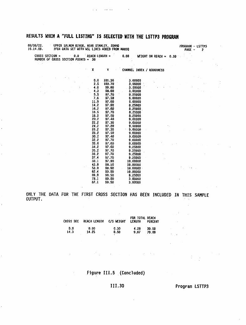
RESULTS IIltEN A "FULL LISTING" IS SELECTED NITH THE LSTTP3 PROGRAM
88/08/22. UPPER SAlMOH RIVER, HEAR STAHlEV, IDAHO16.14.09. IFG4 DATA SET WITH WSl liNES ADOED FROM MAHSQ
CROSS SECTION - 0.0 REACH lENGTH - 0.00NUH8ER OF CROSS SECTION POINTS- 3D
IlEIGHT ON REACH. 0.30
PROGRAH - lSTTP3PAGE - 2
x y CHANNEL INDEX / ROUGNNESS
0.0 101.30 3.000002.5 100.70 3.000004.0 91}.60 3.0DOOO4.3 98.60 3.0QOOO5.5 97.70 9.250007.6 97.30 6.00000
11.9 97.60 6.DOOOO14.2 87.80 8.2500016.2 91.60 8.2500016.5 97.10 8.2500018.2 97.50 8.2500020.2 97.40 9.0000022.2 97.30 9.0000024.2 97.20 9.0000026.2 97.30 9.0000026.2 97.50 9.0000030.2 97.40 8.0000032.2 97.70 9.0000033.0 97.60 8.0000034.2 91.60 9.2500035.2 97.10 9.250003U 87.70 9.2500037.4 91.70 9.2500039.1 97.80 10.0000043.6 98.10 10.0000053.0 96.60 10.0000062,4 98.00 10.0000068.8 88.50 8.2500078.1 99.00 3.0000087.1 99.50 3.00000
ONLY THE DATA FOR THE FIRST CROSS SECTION HAS BEEN INCLUDED IN THIS SAMPLEOUTPUT.
FOR TOTAL REACHCROSS SEC REACH lENGTH CIS WEIGHT LENGTH PERCENT
0.014.3
0.0014.25
0.300.50
4.28 30.009.97 70.00
Figur(! III.5 (Concluded)
III.30 Program LSTTP3

LSTTP4 Program
I. INTRODUCTION
The LSTTP4 program lists the contents of aTAPE4 file. The program alsowill list the contents of a TP4, TAPE4A, or TP4A file. These files areunformatted files containing flow data generated by the hydraul ic simul ationprograms and used as input to the habitat simulation programs.
LSTTP4 output contains the predicted water surface elevation for each flowin a cross section. The slope is also listed if Option 9-T in the WSP program(writes the calculated slope to the TAPE4 as an additional variable). If Option9=T in WSP, the resulting TAPE4 cannot be used as input to the habitat simulationprograms.
II. RUNNING LSTTP4
RLSTTP4,ZOUT.TAPE4
ZOUT-LSTTP4 results (output)TAPE4=unformatted flow data (input)
DO VOU WANT VELOCITIES TO BE LISTED? VIN
If nv" is selected to list velocities. the velocity for each cell in across section is also listed.
Figure [11.6 contains sample output from the LSTTP4 program.
RESULTS OF THE LSTTP4 PROGRAM WHEN VELOCITIES ARE NOT LISTED
CROSS SEcnOR • 0.0 Q. 8.00 WSL = 97.080
CROSS SECTlOR = 0.0 Q. 10.00 WSL It 97.720
CROSS SECTlOR • 0.0 Q= 20.00 WSL = 97.840
CROSS SECTloR • 0.0 Q. 30.00 WSL· 97.930
CROSS SECTloR • 0.0 Q. 40.00 WSL • 98.010
CROSS SECTloR • 0.0 Q. 50.00 WSL • 98.080
CROSS SECT lOR • 0.0 Q= 80.00 WSL • 98.130
ONLY PART OF THE DATA FOR THE FIRST CROSS SECTION HAS BEEN INCLUDED IN THISSAMPLE OUTPUT.
Figure 111.6. Sample output from the LSTTP4 program.
111.31 Program LSTTP4

RESULTS OF THE LSTTP4 PROGRAM WHEN SLOPES WERE WRITTEN TO THE TAPE4BY SETTING OPTION 9.T IN THE WSP PROGRAM
CROSS SECTION • 0.0 Q• 30.00 WSL .u 98.900SLOPE • 0.000687
CROSS SECTION • 18.3 Q• 30.00 lISL- 98.917SLOPE • 0.000055
CROSS SEcnON • 25.S Q • 30.00 WSl Ill: 98.917SLOPE· 0.000105
CROSS SECTION' 34.8 Q• 30.00 WSl '" 98.925SLOPE • 0.000011
RESULTS OF THE LSTTP4 PROGRAM WHEN VELOCITIES ~RE LISTED
CROSS SECTION • 0.0 Q • 8.00 NUM8ER OF VELOCITIES. 18WSL • 97.680
THE VELOCITIES ARE -0.46 0.62 0.16 0.16 0.16 0.62 1.511.59 1.78 2.22 1.90 1.40 0.63 0.420.54 0.12
CROSS SECTION • 0.0 Q• 10.00 NUMBER OF VELOCITIES • 20WSL • 97.720
THE VELOCITIES ARE •0.03 0.52 0.69 0.21 0.21 0.27 0.761.67 1.71 1.87 2.33 2.07 1.56 0.960.81 0.70 0.20 0.18 0.26 0.13
CROSS SECTION • 0.0 Q. 20.00 NUM8ER or VELOCITIES • 20WSL • 97.840
THE VELOCITIES ARE .0.14 0.78 1.00 0.37 0.37 0.62 l.302.37 2.30 2.41 3.02 2.87 2.24 2.052.06 1.23 0.4B 0.72 1.07 0.54
CROSS SECTION • 0.0 Q• 30.00 NUMBER or VELOCITIES • 21WSL • 97.930
THE VELOCITIES ARE .0.21 0.95 1.22 0.5B 0.58 0.86 1.662.B7 2.72 2.79 3.50 3.44 2.72 2.752.6B . 1.61 0.62 1.05 1.58 0.99 0.20
ONLY PART OF THE DATA FOR THE FIRST CROSS SECTION HAS BEEN INCLUDED IN THISSAMPLE OUTPUT.
Figure III.6. (Concluded)
II I. 32 Program lSTTP4

LSTVD Program
I. INTRODUCTION
The LSTVD program lists the velocities and depths of the cells, and crosssection data that are found on a TAPE3 and TAPE4 (a TP4, TAPE4A, or TP4A can beused in place of a TAP(4). ATAPE3 file is an unformatted file containing crosssection and reach data; and a TAPE4 (TP4, TAPE4A, or TP4A) is an unformatted filecontaining flow data. These files are generated by the hydraulic si~ulation
programs and are used as input to the habitat simulation programs.
II. RUNNING LSTVD
RLSTVD,ZOUT,TAPE3.TAPE4
ZOUT=LSTVD results (output)TAPE3=unformatted cross section and reach data (input)TAPE4=unformatted flow data (input)
ENTER HOW VELOCITIES WERE WRITTEN ON TAPE4:i) AVERAGE OF THE VELOCITIES FOR A CELL DEFINED BY ADJACENT
VERTICALS (HABTAT) ._2) VELOCITIES FOR ACELL CENTERED ON AVERTICAL (HASTAM, HABTAV)
Option 2 would be entered if the TAPE4 (which should have been renamedTAPE4A by the user) was created by setting IOC(i7)-l in IFG4;settingIOC(ll)-2 in MANSQ; or created by the .OIRI4 program using Option 1•.
Figure 111.7 contains sample output from the LSTVD program.
1[1.33 Program LSTVD

88/08115. UPPER SAt!1ON RIVER. NEAR STANLEY. IDAHO PROGRAH·LSTYO12.10.12. IFG4 DATA SET VITH WSL LINES ADDED FRPH MANSQ PAGE 2
COORDINATE DATA FOR CROSS SECTION - 0.00 SECTION NO. - 1
X 0.0 2.5 4.0 4.3 5.5 1.6 11.9 14.2 16.2 16.5 18.2 20.2Y 101.3 100.7 99.8 98.6 97.1 97.3 97.8 97;9 97.6 97.7 97.5 97.4S 3.0 . 3.0 3.0 3.0 9.2 6.0 6.0 8.2 8.2 8.2 .8.2 9.0
X 22.2 24.2 26.2 28.2 30.2 32.2 33.0 34.2 35.2 36.2 37.4 39.1Y 97.3 97.2 97.3 97.5 97.4 97.7 97.6 97.6 97.7 97.7 97.7 97.9S 9.0 9.0 9.0 9.0 9.0 9.0 9.0 9.2 9.2 9.2 9.2 10.0
X 43.6 53.0 62.4 . 69.9 78.1 87.1Y 96.1 98.6 99.0 96.5 99.0 99.5S 10.0 10.0 10.0 8.2 3.0 3.0
STREAM DISCHARGE IS 8.0 CUSECS VSL IS 97.68 FEET
0 0.0 0.0 0.0 0.0 0.2 0.2 0.0 0.0 0.0 0.1 0.2 0.3V 0.00 0.00 0.00 0.00 0.46 0.62 0.16 0.16 0.16 0.62 1.51 1.59
0 0.4 0.4 0.3 0.2 0.1 0.0 0.1 0.0 0.0 0.0 0.0 0.0V 1.76 2.22 1.90 1.40 0.63 0.42 0.54 0.12 0.00 0.00 0.00 0.00
0 0.0 0.0 0.0 0.0 0.0V 0.00 0.00 0.00 0.00 0.00
STREAM DISCHARGE IS 10.0 CUSECS WSL IS 91.12 FEET
0 0.0 0.0 0.0 0;0 0.2 0.3 0.1 0.1 0.1 0.1 0.3 0.4V 0.00 0.00 0.00 0.03 0.52 0.69 0.21 0.21 0.27 0.76 1.61 1.71
0 0.5 0.5 0.3 0.3 0.2 0.1 0.1 0.1 0.0 0.0 0.0 0.0V 1.61 2.33 2.07 1.56 0.96 0.81 0.70 0.20 0.16 0.26 0.13 • 0.00
0 0.0 0.0 0.0 0.0 0.0V 0.00 0.00 0.00 0.00 0.00
REMAINING OUTPUT WAS TERMINTATEO HERE FOR BREVITY.
Figure 111.7. Sample output from the LSTVO program.
II I.34 Program LSTVO

LSTWLF Program
I. INTRODUCTION
The LSTWLF program 1ists. water surface elevations on a TAPE4, andcalculates and lists the Froude number and mean channel velocities for each cross
. sect ion and each flow. A TAPE3 fil e is an unformatted fil e conta ini ng crosssection and reach data; and a TAPE4 (TP4, TAPE4A, or TP4A) is an unformatted filecontaining flow data. These files are generated by the hydraul ic simul ationprograms and are used as input to the habitat simulation programs.
II. RUNNING LSTWLF
RLSTWLF, ZOUT.TAPE3.TAPE4
ZOUTaLSTWLF results (output)TAPE3=unformatted cross section and reach data (input)TAPE4=unformatted flow data (input)
The definitions of the terms given on the output from LSTWLF are givenbelow:
DISTANCE: The di stance from the most downstream cross sect ion to the nextupstream cross section.
THALWEG: The elevation of the low point in the cross section.
VEL (Mean Channel Velocity): The velocity calculated by dividing the dischargeby the cross-sectional area.
CVEL (Celerity): . The velocity of agravity wave in the channel at the givenwater surface elevation. The celerity is given by the equation
CVELa f90
where 9 is the acceleration of gravity and d is the depth calculated bythe equation
d = Q/W
where Q is the discharge and Wis the surface width at the given watersurface elevation. The celerity then becomes
CVEL = /9ll7IY
FRQUPE NUMBER: The ratio of the mean channel velocity to the celerity. If theFroude number is <l.0. the flow is sub-critical (slow); and if it is >1.0. theflow is super-critical (fast). A Froude number of 1.0 is crit!cal flow.
Figure 111.8 contains sample output from the LSTWLF program.
III. 35 Program lSTWLF
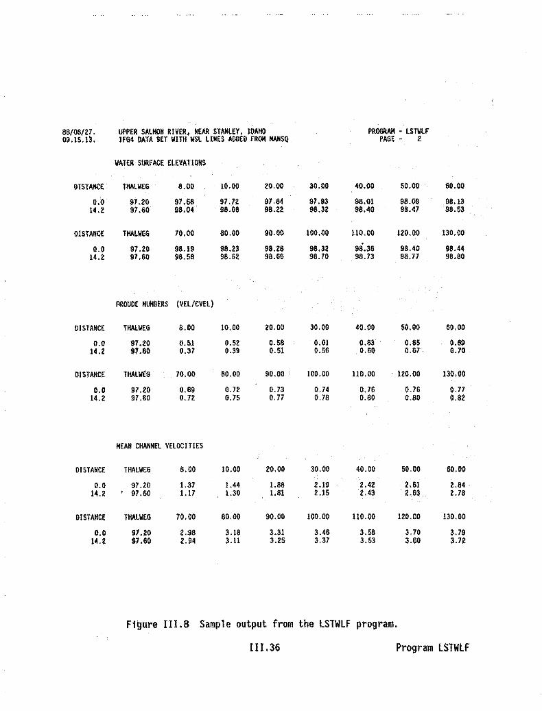
88/08/27. UPPER SALKON RIVER. NEAR STANLEV. IDAHO PROGRIlM - LSM,09.15.13. IFG4 DATA SET WITH W5L LINES ADOED FROM MANSO PAGE - 2
WATER SURFACE ELEVATIONS
915TAlICE THAL\lfG 8.00 10.90 20.00 30.09 40.09 50.09 80.00
9.0 91.20 97.88 91.72 97.84 97.93 96.01 96.06 98.1314.2 97.80 98.04 98.08 98.22 98.32 98.40 98.47 98.53
DISTANCE THAl\lfG 70.00 80.09 90.00 100.00 110.00 129.99 130.00
0.0 97.29 98.19 98.23 96.28 98.32 98.36 98.40 98.4414.2 97.60 98.58 96.62 98.66 98.70 98.73 98.77 98.80
FROUDE HUII8ERS (VEL/CVEl)
DISTANCE THAl\lfO 8.00 10.00 20.00 30.00 40.00 50.00 60,00
0.0 91.20 0.51 0.52 0.58 0.61 0.63 0.65 0.6914.2 97.80 9.37 0.39 0.51 0.56 0.60 0.67 0.70
olSTIlMCE THAlIltG 70.00 80.09 90.00 109.00 110.00 120.00 130.00
0.0 97.20 0.69 0.72 0.73 0.74 0.76 0.76 0.7714.2 97.69 0.72 0.75 0.77 0.78 0.80 0.60 0.82
MEAN CHANNEL VELOCITIES
01 STANCE THALWE6 8.00 10.09 20.00 30.00 40.00 50.00 60.00
0.0 97.20 1.37 1.44 1.86 2.19 2.42 2.61 2.8414.2 • 97.80 1.17 1.30 1.81 2.15 2.43 2.63 2.78
DISTANCE THAll/(O 70.00 80.09 90.09 190.00 110.00 120.00 139.00
0.0 97.20 2.96 3.18 3.31 3.46 3.58 3,70 3.7914.2 97.60 2.94 3.11 3.25 3.37 3.53 3.60 3.72
Figure 111.6 Sample output from the lSTWlF program.
II I. 36 Program lSTWlF

HODCI Program
I. INTRODUCTION
The MODCI program adds or modifies channel index data, reach lengths, andweighting factors in a TAPE3. Option of entering data from the keyboard orreading data from a file created by ENTCI.
This program is generally run when the TAPE3 resulting from a WSP run isto be used as input to the habitat simulation programs. Channel index valuesare not included in a WSP data set; thus they are not passed onto the TAPE3(channel index values of "0" are written to the TAPE3 by WSP). Channel indexvalues are used in the calculation of Weighted Usable Area (WUA) in habitatsimulation.
II. RUNNING MODCI
RMODCI,TAPE3,TAPE3N,ZCHANF
TAPE3~unformatted cross section and reach data (input)TAPE3N=modified TAPE3 file with channel index data added (output)ZCHANF=file containing channel index data (input).This file was created by the ENTCI program.
ENTER 0 TO READ DATA FROM FILE CREATED BY ENTCI,ENTER 1 TO INPUT DATA FROM KEYBOARD:
The following series of prompts will appear if data Is being entered from thekevboard:
THE CROSS SECTION 10 NUMBER IS _.. :WEIGHT FOR CROSS SECTION IS ---:(ENTER NEW WEIGHT OR -I TO LEAVE AS IS):
REACH LENGTH FOR CROSS SECTION -.. IS ---;(ENTER NEW REACH LENGTH OR -1 TO LEAVE AS IS):
NUMBER OF CHANNEL INDEX VALUES FOR CROSS SECTION -_. IS --.:ENTER .- NEW CHANNEL INDEX VALUES,OR 0 FOR NO CHANGE IN THE CHANNEL INDEX VALUES FOR THE CROSS SECTION:
III.37 Program MODCI
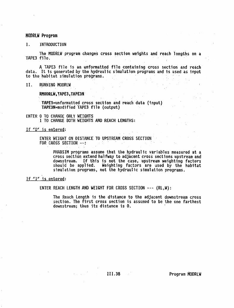
MODRUI Program
I. INTRODUCTION
The MODRlW program changes cross section weights and reach lengths on aTAPE3 file.
A TAPE3 file is an unformatted file containing cross section and reachdata. It is generated by the hydraulic simulation programs and is used as inputto the habitat simulation programs.
II. RUNNING MODRLW
RHODRLW.TAPE3.TAPE3N
TAPE3~unformatted cross section and reach data (input)TAPE3N~modjfied TAPE3 file (output)
ENTER 0 TO CHANGE ONLY WEIGHTSI TO CHANGE BOTH WEIGHTS AND REACH LENGTHS:
If "0" is entered:
ENTER WEIGHT ON DISTANCE TO UPSTREAM CROSS SECTIONFOR CROSS SECTION _.:
PHABSIM programs assume that the hydraulic variables measured at across sectiOn extend halfway to adjacent .cross sections upstream anddownstream. If this is not the case. upstream weighting factorsshould be applied. Weighting factors are used by the habitatsimulation programs, not the hydraulic simulation programs.
If "1" is entered:
ENTER REACH LENGTH AND WEIGHT FOR CROSS SECTION --- (RL,W):
The Reach Length is the distance to the adjacent downstream crosssection. The first cross section is assumed to be the one farthestdownstream; thus its distance is O. .
III. 38 Program MODRlW

RPHABAR Batch/Procedure File
I. INTRODUCTION
The RPHA8AR batch/llrocedure file runs either the PHABAR2 or PHABARRprograms to rearrange a TAPE4 and writes a TP4. The user will not normally runthis procedure as the RIFG4, RWSP, and ROIRI4 batch/procedure files automaticallyrun the PHABAR2 program for you.
The hydraulic simulation program output for all flo~s is arranged by ,crosssection. The computational procedure develops the water surface elevations andvelocities for one cross section, writes those data for all flows at that sectionto TAPE4, then moves to the next cross section, and so forth through the reach.In contrast, the habitat simulation programs require that the hydraulic data forall the cross sections in the reach be available one flow at a time. The PHABARRand PHABAR2 programs rearrange the TAPE4 output from the hydraulic programs intothe format required by the habitat simulation programs and write it on TP4.
II. RUNNING THE RPHABAR BATCH/PROCEDURE FILE
RPHABAR.TAPE4,TP4.POS
TAPE4=unformatted flow data (input)TP4=rearranged TAPE4 file (output)PUS. -1 leaves negative velocities as negative numbers (PHABARR)POS. 1 Converts negative velocities to positive numbers (PHABAR2)
Default is POS-l (PHABAR2).Run by the RIFG4, RWSP, and RDIRI4 batch/procedures files.
II I.39 Batch/Procedure File RPHABAR

PHARRIN ProgramI. INTRODUCTION
The PHABRTN program converts a TP4 file back to a TAPE4 file. TP4 is arearranged TAPE4 file created by the PHABAR2 program when the RIFG4, RWSP, orRDIRI4 batch/procedures files are run. TAPE4 and TP4 contain unformatted flowdata. TP4A can also be converted back to TAPE4A.
The hydraulic simulation program output for all flows is arranged by crosssection. The computational procedure develops the water surface elevations andvelocities for one cross section, writes those data for all flows at that sectionto TAPE4, then moves to the next cross section, and so forth through .the reach.In contrast, the habitat simulation programs require that the hydraulic data forall the cross sections in the reach be avail able one flow ata time. The PHABARRand PHABARZ programs rearrange the TAPE4 output from the hydraulic programs intothe format required by the habitat simulation programs and write it on TP4.
II. RUNNING PHABRTN
RPHBRTN,TP4,TAPE4
TP4-rearranged TAPE4 file of unformatted flow data (input)TAPE4-unformatted flow data (output)
mAo Program PHABRTN

UTP34F Program
I. INTRODUCTION
The UTP34F program converts an unformatted TAPE30r TAPE4 to a formattedTAPE3F or TAPE4F.
A TAPE3 file is an unformatted ffle containing cross sllctfon and reachdata, and a TAPE4 (TP4, TAPE4A, or TP4A) is an unformatted file containing flowdata. These files are generated by the hydraulic simulation programs and are usedas input to the habitat simUlation programs.
Unformatted files are likely to be incompatible between a microcomputerand the COC mainframe, and between different microcomputers. The formattedversion of the files should be used when transferring from computer to computer.
II. RUNNING UTP34F
RUTP34F.TAPE3.TAPE3F,TAPE4.TAPE4F
(if only a TAPE4 is ·to be converted,use: RUTP34F,TAPE4,TAPE4F)
TAPE3=unformatted cross section and reach data (input)TAPE3F=formatted cross section and reach data (output)TAPE4=unformatted flow data (input)TAPE4F=formatted flow data (output)
UI.41 Program UTP34F

IV. CRITERIA CURVE MAINTENANCE PROGRAMS
INTRODUCTION
In order to evaluate the magnitude of impacts caused by changes in streamhydraulics, it is necessary to develop an information base for each species orgroup of species of interest. The information base is in the form of criteriacurves of aquatic species or recreational activities.
Biological criteria are primarily aimed at those parameters affecting fishdistribution which are directlY related to streamflow and channel morphology;specifically depth, velocity, temperature, and channel index. Cover, a habitatparameter of paramount importance to many species, is also indirectly relatedto streamflow. Cover may be incorporated into an assessment by evaluating theusability of available cover objects in reference to the flow parameters aroundthem.
The expressed assumption is that the distribution and abundance of anyspecies is not primarily influenced by any single parameter of streamflow. butis related by varying degrees to all streamflow hydraulic parameters.Furthermore. these criteria are based on the assumption that individuals of aspecies tend to select the most favorable conditions in a stream, but will alsouse less favorable conditions, with the preference for use decreasing whereconditions are less favorable.
Agroup of curve maintenance programs has been developed to manage a fileof criteria curves of aquatie species or recreational activities. Figure 1.7contains information on the "Flow of Information Through PHABSIM . CurveMaintenance Programs Group".
In this documentation, the term FISHeRV refers to the formatted (cardimage) version of the file containing the curve sets created by the GCURV programor by using an editor. The term FISHFIl refers to the unformatted (binary)version of the file created by the CRVFIL program. The unformatted version ofthe file is used as an input to the habitat simulation programs.
The formatted version of the curves file can be thought of as a librarywhere curves are filed by identification number. This file should be saved and
.. may be added to as new curves are entered.
IV.I

~Rm.R.IA CYR.YE DATA mRY, REVIEll, AHILPLOTTING PROGRAI'IS
PROGRAM BATCH/PROCEDURENAME FILENAME FUNCTIQB PROGRAM DESCRIPTION
SCURY RGCURY Criteria Curve Builds a formatted FISHCRY file fromData Entry keyboard input.
RGCURV,FISHCRV
FISHCRV-formatted curves fi 1e (output)
LPTCRY RLPTCRV Cri teria CurveReview andPlotting
Checks data contained in a formattedFISHCRY file with option to generategraphs from the curve data.
RlPTCRY,FISHCRV,ZOUT
FISHeRV-formatted curves fi 1e (i nput)ZOUT-lPTCRV results (output)
PROGRAMS USED HITlJ fORMAnED (FISHeRY) CURVES FILES .
CRYFIl RCRVFIl Criteria Curve Converts a formatted FISHCRV file toConversion an unformatted FISHFIl file.
CRY2LOT RCRV2LT
RCRYFIL,FISHeRV,FISHFIL
FISHCRY=formatted curves file (input)FISHFIl=unformatted curves file(output)
Criteria Curve Converts a formatted FISHCRV file toConversion a file that is readable by LOTUS.
RCRV2LT,FISHCRY,ZOUT
FISHCRY=formatted curves file (input)ZOUT=LOTUS readable curves file(output)
IV.2

PBOGRA~ USED IIITH FORlWIfD (FISHCRY) CUl\V£S mES (Continued)
BATCH/PROCEDUREFILENAME FUNCTION
PROGRAMNAME
EXCRVS
LSTH
REXCRVS
RLSTH
Criteria CurveManipulation
Cri teri a Curveli sting
PROGRAM DESCRIPTION
Extracts specified curve sets from aformatted FISHCRV file and writes theextracted curves to a new file inFISHCRV format.
REXCRVS, FISHCRY ,NEWFCRV
FISHCRY=formatted curves file (input)NEWFCRY=new formatted curves file(output)
Lists the header lines in a formattedFISHeRV fi1 e.
RLSTH,FISHCRV,ZOUT
FISHCRV"formatted curves file (i nput)ZOUT=lSTH results (output) (iffilename is not specified, outputwill go to the screen)
PROGRAMS USED WITH UNFORMATTED' (FISHFILl CURVES FILES
CRVWRT RCRVWItT Criteri.a Curve Converts an unformatted fISHFIl fil eConversion to a formatted FISHCRV file.
LDIR RLDIR Cri teri a Curvelisting
IV.3
RCRYWRT.FISHFIL.FISHCRY
FISHFIl=unformatted curves file(input)
FIS!lCRY"formatted curves fll e (output)
\lri tes a complete or partia1 di rectorylisting of an unformatted FISHFIL.
RLDIR.FISHFIl.ZOUT
FISHFIl=unformatted curves file(input)
ZOUT=lDIR results (output) (iffilename not specified. output willgo to the screen)

PROGRAM DESCRIPTIQH
PROGRAMS USED WITH UN~ORMATTED (~ISH~Jl) CURVES FILES (Continued]
PROGRAM BATCH/PROCEDURENAME FILENAME FUNCTION
LSTCNUM RLSTCNM
Criteria CurveListing
LSTCRV RLSTCRV
Criteria Curve lists the curve set 10 numbers in anListing unformatted FISHFIL file.
RlSTCNM,FISHFIL,ZOUT
FISHFIL-unformatted curves file(input)
lOUT-LSTCNUM results (output) (iffilename is not specified, outputwill go to the screen)
Lists the coordinates of the curvesin a FISHFIL file for up to 40 1ifestages.
RlSTCRV,FISHFIl,lOUT,ZHABIN
FISHElL-unformatted curves file(input)
lOUT-curve coordinates from FISHFIl(output)
ZHABIN-HABTAT, HABTAV, HABTAM, HABTAE,or HABVO options file, optional(input). If specified, the curveset 10 numbers on the CURVES linein the options file will bedi splayed; the user will be promptedto enter how many of these curve setsto process and the curve set 10numbers.
IVA

CRV2LOT Program
I. INTRODUCTION
The.CRV2LOT program converts a formatted FISHCRV file to a file that isreadable by LOTUS. Since the number.of coordinate pairs may vary, all columnsare as long as the longest record with zero fills in the columns not filled Withcurve data. If temperature sUitability is not present, temperature columns arezero filled.
II. RUNNING CRV2l0T
RCRV2lT ,FISHCRY, ZOUT
FISHCRV=formatted curves file (input)ZOUT=lOTUS readable curves file (output)
CONVERTING ASCII TEXT CURVES FILE TO LOTUS READABLE FORMAT:
END OF INFORMATION FOUND, All CURVES HAVE BEEN WRITTEN TO FILE.
Figure IV.I contains sample output from the CRV2l0T program.
'H 11119 9 9 7 0 WINTER TROUT ADULT 88/04/25
• ·.·VElOCIT~·.· ·.·OEPTH'.· CHANNEl··DESCRPT.·.· TEMPERATURE'0.00 l.00 0.00 0.00 0.00 0.00 0.00 0.000.20 1.00 0.50 0.05 3.90 0.00 0.00 0.000.30 0.80 0.75 0.10 4.00 1.00 0.00 0.000.50 0.50 1.00 0.25 7.00 1.00 0.00 0.000.75 0.20 1.25 0.50 8.00 0.50 0.00 0.001.00 0.15 1.50 0.75 9.00 0.00 0.00 0.001.50 0.10 1.75 1.00 100.00 0.00 0.00 0.002.00 0.00 4.00 l.00 0.00 0.00 0.00 0.00
100.00 0.00 100.00 1.00 0.00 0.00 0.00 0.00
'H 11112 4 7 8 ,0 BROWN TROUT FRY
• ·.·VELOCITY·.· ·.·OEPTH·.· CHANNEl··OESCRPT.·.· TEMPERATURE'0.00 1.00 0.00 0.00 0.00 l.00 0.00 0.000.10 1.00 0.10 0.10 l.00 l.00 0.00 0.000.50 0.00 0.20 l.00 2.00 l.00 0.00 0.00
100.00 0.00 0.50 l.00 4.00 l.00 0.00 0.000.00 0.00 1.25 0.30 6.00 1.00 0.00 0.000.00 0.00 3.00 0.00 8.00' 1.00 0.00 0.000.00 0.00 100.00 0.00 9.00 1.00 0.00 0.000.00 0.00 0.00 0.00 100.00 l.00 0.00 0.00
Figure IV.I. Sample output from the CRV2l0T program.
IV.5 Program CRV2l0T

CRVrIl Program
I. INTRODUCTION
The CRVFI L program converts a formatted FISHCRV fll e to an unformattedFISHFIL file. The FISHFIL is used as input to the habitat simulation programs.
Unformatted files, such as FISHFIL, are likely to be incompatible betweena microcomputer and the CDC mainframe, and between different microcomputers.The formatted version (FISHCRV) of the files should be used when transferringfrom computer to computer.
II. RUNNING CRVFIL
RCRVFIl,FISHCRV,FISHFIl
FISHCRV=formatted curves file (input)FISHFIL=unformatted curves file (output)
A directory of the FISHFIL will print out on the screen.
IV.6 Program CRVFIL

CRVWRT Program
I. INTRODUCTION
The CRVWRT program converts an .unformatted FlSHFIl file to a formattedFISHCRV file. This program is not normally used,as it is reco1l111ended that theformatted (card image) version of the file be saved and added to as new curvesare entered.
Unformatted files, such as FISHFIl, are likely to be incompatible betweena microcomputer and the CDC mainframe, and between different microcomputers.The formatted version (FISHCRY) of the files should be used when transferringfrom computer to computer.
II. RUNNING CRVWRT
RCRVWRT,FISHFIL,FISHCRV
FISHFIL~unformatted curves file (input)FISHCRycformatted curves file (output)
IV.7 Program CRVWRT

EXCRVS ProgramI. INTRODUCTION
The EXCRVS program extracts specified curve sets from a FISHCRV file andwrites the extracted curves to a new file in FiSHCRV format.
II, RUNNiNG EXCRVS
REXCRVS,FISHCRV,NEWFCRV
FISHeRV-formatted curves file (input)NEWFCRV-new formatted curves file (output)
ENTER NUMBER OF CURVE SETS TO EXTRACT:
ENTER THE CURVE SET 10 NUMBER(S):
ENTER TITLE LiNE FOR NEW FISHCRV FILE (70 CHARS MAX)?
Alisting of the header lines in the new FISHCRV file will print outon the screen.
IV.S Program EXCRVS

GCURV Program
I. INTRODUCTION
The GCURV program builds a FISHCRV file containing criteria curves ofaquatic species or recreational activities. This file can be edited with aneditor to correct errors or for modifications. The LPTCRV program checks thedata contained in a FISHCRV file for errors. After correcting errors identifiedby running LPTCRV, convert the FISHCRV file to an unformatted FISHFIL by usingthe CRVFIL program. The unformatted FISHFIL is used as input to the habitatsimulation programs.
Appendix Acontains the file format for a FISHCRV file and a sample FISHCRVfile.
II. RUNNING GCURV
RGCURV,FISHCRV
FISHCRV=formatted curves file (output)
ENTER THE TITLE FOR THE FILE (70 CHARS MAX):
NUMBER OF CURVE SETS TO BE ENTERED (60 MAX):
ENTER CURVE SET 10 NUMBERS:
Six-digit identification numbers for family, species. and lifestage.
NUMBER OF POINTS FOR VELOCITY CURVE:
When entering curve coordinate data for velocity, depth, and channel index.each curve must begin with a minimum X value of 0 and should end with amaximum Xvalue of 100.
NUMBER OF POINTS FOR DEPTH CURVE:
NUMBER OF POINTS FOR CHANNEL INDEX CURVE:
NUMBER OF POINTS FOR TEMPERATURE CURVE:
SPECIES DESCRIPTOR (40 CHARS MAX):
LIFE STAGE DESCRIPTOR (8 CHARS MAX):
ENTER -- VELOCITY COORDINATE PAIRS (V,SI):
ENTER -- DEPTH COORDINATE PAIRS (D,SI):
ENTER .. CHANNEL INDEX COORDINATE PAIRS (S,SI):
IV.9 Program GCURV

LDIR Program
I. INTRODUCTION
TheLDIR program writes a complete or partial directory listing of anunformattedFISHFIL.
II. RUNNING LDIR
RLDIR,FISHFIL,ZOUT
FISHFIL~unformatted curves file (input)ZOUT=LDIR results (output) (if filename is not specified,output will go to the screen)
FOR A COMPLETE LISTING OF THE CURVE DIRECTORY ENTER I.FOR A PARTIAL LISTING ENTER O.
Figure IV.2 contains sample output from the LDIR program. A partialdirectory listing and a complete.directory listing is included.
IV.IO Program LDIR

PARTIAL DIRECTORY LISTING FROM THE LDIR PROGRAM
CIJlV£ FILE TITLE -SAMPLE FISHCRV FILE CREATED WITH THE GCURV .PROGRAM
HUMllER OF CURVES- 11DATE AND TIME LAST MOllIFIED OR CREATED- 88/07114. 11.28.32.
lD LIFENUMBER SPECIES STAGE DATE
I 11119 \lINTER TROUT ADULT 88/0T!14.2 11112 BROIIH TROUT FRY 88/07/14.3 11114 BROIIH TROUT JUVENILE 88/07/14.4 Jl11S BROIIH TROUT ADULT 86/07/14.5 11120 BROWN TROUT SPAWNING 88/07/14.8 1I12B BROlIN/RAINBOW COlO WEATHER EGGS 88/07/14.7 11127 BROIIH/RAINBOW TROUT HILD WINTER EGG 86/07114.8 21110 RAINBOW TROUT SPAWNING 8B/07/14.9 21112 RAINBOW TRoUT FRY 88/07/14.
10 21114 RAI NBOW TROUT JUVENILE 88/07/14.11 21115 RAI NBOW TROUT ADULT 8B/07114.
11 CURVES IN FILE.
COMPLETE DIRECTORY LISTING FROM THE LDIR PROGRAM
CURVE FILE TITLE -SAMPLE FISHeRV FILE CREATED WITH THE GCURV PROGRAM
NuNBER OF CURVES- IIDATE AND TINE LAST MODIFIED OR CREATED- 86/07/14. 11.28.32.,
DIRECTORY FOR THE HA81TAT PREFERENCE CURVE FILE 88/07/14. 11.28.32. PAGE I
10 LIFE NO. OF POINTS USEO INSTALLATION TOTALNUMBER SPECIES STAGE VEL DEP SU8S TEMP DATE POINTS
I. 11119 WINTER TROUT ADULT 9 9 7 0 88/07114. 2G.002. 11112 BROIIH TROUT FRY 4 7 8 0 88/07/14. 19.003. 11114 8ROIIH TROUT JUVENILE 6 3 8 0 B8/07/14. 17.004. IlliG BROlIN TROUT ADULT 5 3 7 0 88/07/14. 15.005. IlI20 BROlIN TROUT SPAWNING 6 4 U 0 88/07/14. 21.006. 11126 BROIIH/RAIN801/ COLO \lEATHER EGGS 5 6 8 0 66/07/14. 19.007. U127 BROIIN/RAINBOI/ TROUT MILO WINTER EGG 4 4 8 0 88/07/14. 16.008. 21110 RAIN801/ TROUT SPAWNING 7 6 U 0 88/07/14. 24.009. 21112 RAIN8~W TROUT FRY 4 B 8 0 88/07/14. 20.00
10. 21114 RAINBOW TROUT JUVENILE 5 4 B 0 8B/07/14. 17.00II. 2lU5 RAINBOW TROUT ADULT 4 4 8 0 88/07/14. 16;00
Figure IV.2. Sample output from the lOIR program.
IV.ll Program LOIR

LPTCRV Program
I. INTRODUCTION
The LPTCRV program checks data contained in a formatted FISHCRV file withthe option to generate graphs from the curve data. The file may have beengenerated by the GCURV program or created with an editor.
II. RUNNING LPTCRV
RLPTCRV,FISHCRV,ZOUT
FISHCRV=formatted curves file (input)ZOUT=LPTCRV results (output)
HQIE: On the microcomputer, graphs may be printed to the screen or to the outputfile using character graphics (132 characters per line format). In orderto use screen graphics, the computer must have a Color Graphics Adaptor(CGA) or compatible graphics card. When using screen graphics, notes arewritten to the output file in the positions where the graphs would havebeen placed had they been written using character graphics.
ENTER 1 TO PLOT CRITERIA, 0 OTHERWISE:
Entering "I" generates the same output as "0" plus the plots.
SEARCH (output filename) FOR $$$ TO LOCATE ERROR MESSAGES.
Notice the errors that are identified on the first page of the sampleLPTCRV output contained in Figure IV.3.
IV.12 Program lPTCRV

The following FISHeRY file was used as input to the tPTCKY program whichresulted in the sample output.
FISHCRY FilE VITH ERRORSH 10102 5 1 4 0 BROVN TROUT - COYERV 10102 0.00 1.00 0.50 1.00 2.00 0.30o 10102 0.00 0.00 0.10 0.00 5.00 1.00a 10102100.00 0.00S 10102 1.00 0.00 2.00 0.80 3.00 0.80
JUVENILE 88/06/16.3.25 0.00100.00 0.002.50 1.00 3.00 0.80 4.00 0.00
4.00 1.00
FROG - LPTCRV 88/06/16. 08.53.11. FISHeRV FilE VITH ERRORS
SET NO. I BROWN TROUT - COVER JUVENILE CURVE NO. 10102
VElOCITY DATA
VELOCITY 0.00 0.50 Z.OO 3.25 100.00SUITA8ILlTY 1.00 1.00 0.30 0.00 0.00
OEPTH OATA
OEPTH 0.00 0.10 5.00 Z.50 3.00 4.00 100.00SUITA81lITY 0.00 0.00 1.00 1.00 0.80 0.00 0.00
U$ ERROR ( 1) X COORO. DONT ASCfIlO ( 5.00 2.SO) 011 THE DEPTH CURVE
CHANNEL INOE~ OATA
CHANNEL INDE~ 1.00 2.00 3.00 4.00SUITA81lITY 0.00 0.80 0.80 1.00
$$$ FIRST POINT HUST Il£ ZERO1.00 VAS fOUNO
$U lAST POINTHUST Il£ 100.04.00 liAS FOUNO
PA6E 1
ONLY THE PLOT OF THE DEPTH CURVE IS INCLUDED IN THIS SAMPLE OUTPUT;NOTICE THAT THE ERRORS ARE NOT IDENTIFIED IN THIS PLOT.
Figure IV.3. Sample output from the LPTCRV program.
IV.I3 Program LPTCRV

I'lO< • U'lCIl\I lI!\Ill6I16. 18.53.17. FlSll:Rl' FILE WITH _ P1a! ~
1.(0)) ., 1 1 1 1 1 1 1 ,, 1 1 1 1 1 1 1 ,, 1 1 1 1 1 1 1 ,, ,0.'lOOOO ,.... ....,, ,, ,, ,, ,o.lroXl ,.... • ....,, ,, ,, ,, ,o.1lOOJ ,.... ....,, ,, ,, ,, ,0.«1:00 ,.... ....,, ,, ,
SUlT/oBIl'Y , ,, ,0.5(0)) ,.... ....,, ,, ,, ,, ,O.«lXIl ,.... ....,, ,, ,, ,, ,03001 ,.... ....,, ,, ,, ,, ,O.aml ,.... , ....,, ,, ,, ,, ,1.00XKIl·01 ,.••• ....,, ,, 1 1 I 1 1 I 1 1 1 ,, 1 1 1 1 1 1 1 1 1 ,, I 1 1 , I 1 1 1 1 ,0.00XKIl·01 -<II' *
0 0_'01 1.(0)) 2.(0)) ~.OO)) 4.(0)) 5.(0))0.5(0)) 1.5000 2.5000 ~.5000 4.5000
IlEPI1l
10002 J.M3lILE 9llWI 1TIWI • CMlt
Figure IV. 3. (Conel uded)
IV.14 Program LPTCRV

LSTCNUH Program
I. INTRODUCTION
The LSTCNUM program 1ists the curve set ro numbers in an unformattedFISHFIL.
II. RUNNING LSTCNUM
RLSTCNM.FlSHFlL.ZOUT
FlSHFIL=unformatted curves file (input)ZOUT=LSTCNUM results (outPllt) (if filename is not specified,output will go to the screen)
The following type of output will appear on the screen or in theoutput file if specified.
THERE ARE1111921110
11 CURVES IN THE FILE. THEY ARE-11112 11114 11115 1112021112 21114 21115
IV.IS
1Il26 IllZ7
Program LSTCNUM

lSTCRV Program
I. INTRODUCTION
The LSTCRV program lists the coordinates of the curves in a FISHFIl filefor up to 40 life stages.
II. RUNNING LSTCRV
RLSTCRV,FISHFIL,ZOUT,ZHABIN,
FISHFIL=unformatted curves file (input)ZOUT=curve coordinates from FISHFIl (output)ZHABIN=HABTAT, HABTAV, HABTAM, HABTAE, or HABVO options file,optional (input). If specified, the curve set 10 numberson the CURVES line in the options file will be displayed;the user will be prompted to enter how many of thesecurve sets to process and the curve set 10 numbers.
Prompts when ZHABIN is specjfied as an jnpyt file:
CURVE SET 10 NUMBERS IN THE FILE ARE-
Curve set 10 numbers from the curves entered on the CURVES line in theoptions file will be listed.
HOW MANY OF THESE CURVE SETS 00 YOU WISH TO PROCESS?
PLEASE LIST THE 10 NUMBERS FOR THE CURVE SETS:
Figure IV.4 contains sample output from the LSTCRV program.
IV.16 Program LSTCRV

CIIlVES 011 THE FILE ARE-11119 UUO
CURVE SET OEFINITIOII DATA WAS OBTAINED FRDM THE FISHFll FILE WHOSE TITLE lINE IS -
SAMPLE FISHCRV FILE CREATED IIITH THE GCURV PROGRAM
lAST UPDATED 011 88/011/01. 09.4I.EI.
IIINTER TROUT ADUlT 11119
VELOCITY DATA
VELOCITY 0.00 D.EO 0.30 O.SO 0.75 1.00 1.50 2.00 100.00SUITABILITY I. DO 1.00 0.80 0.50 O.EO D.l5 0.10 0.00 0.00
DEPTH DATA
DEPTH -- 0.00 O.SO . 0.75 1.00 I.ES LSD loTS 4.DO 100.00SUITABILITY 0.00 0.05 0.10 0.E5 0.50 0.75 1.00 1.00 1.00
CHANNEL INOEX DATA
CHANNEL INDEX 0.00 3.90 4.00 7.00 8.00 9.00 100.00SUITABILITY O.DO 0.00 1.00 1.00 0.50 0.00 0.00
RAINOOl/ TROUT SPAWNING EIllO
VELOCITY DATA
VELOCITY 0.00 0.50 1.30 1.40 2.00 3.20 100.00SUITABILITY 0.00 O.DO 0.95 1.00 1.00 0.00 0.00
DEPTH DATA
DEPTH O.DO 0.30 0.70 2.00 8.DO 100.00SUITABILITY 0.00 0.00 1.00 1.00 0.00 0.00
CHANNEL INDEX DATA
CHANNEL INDEX 0.00 l.OD 2.00 3.00 4.00 5.00 B.DO 7.00 8.009.00
SUITABILITY 0.00 0.00 1.00 1.00 1.00 0.10 0.00 0.00 0.000.00
CHANNEL INDEX 100.00SUlTABILITT 0.00
NORMAL END OF JOB
Figure IV.4. Sample. output from the LSTCRV program.
IV.17 Program LSTCRV

LSTH Program
I. INTRODUCTION
The lSTH program lists the header lines in a formatted FISHeRV file.
II. RUNNING lSTH
RlSTH,FISHCRV,ZOUT
FISHCRV=formatted curves file (input)ZOUT=lSTH results (output) (if filename Is not specified,output will go to the screen)
The following output·will appear on the screen or in the output file ifan output filename is specified.
TITLE OF FILE IS -
SAMPLE FISHCRV FILE CREATEO WITH THE GCURV PROGRAM
NO. OF POINTS LIFE10 VEL OEP CI TEMP SPECIES STAGE DATE
11119 9 9 7 o WINTER TROUT ADULT 88/04/Z5IlI1Z 4 7 8 o BROWN TROUT FRYI1Il4 6 3 8 o BROWN TROUT JUVENILE!l115 5 3 7 o BROWN TROUT ADULT11120 6 411 o BROWN TROUT SPAWNING11126 5 6 8 o BROWN/RAINBOW COLD WEATHER EGG511127 4 4 B o BROWN/RAINBOW NILD WINTER EGG21110 7 6 11 a RAINBOW TROUT SPAWNING21112 4 a a a RAINGOW TROUT FRY21114 5 4 8 o RAIN80W TROUT JUVENILE21115 4 4 8 o RAINBOW TROUT ADULT
II CURVE SETS IN FILE
IV.18 Program lSTH
V. HABITAT SIMULATION PROGRAMS
INTRODUCTION
The following programs are microhabitat simulation models that simulatethe physical habitat for an aquatic species or the recreational space availablefor specific types of recreational activities. The data used are t~e habitatsUitability curves, stream channel geometry, ,water surface elevations, and meancell velocities of the stream.
The stream is broken down into a series of rectangular cells. the lengthand width of which are determined by the reach length stationing and thecross-sectional stationing. respectivelY, as entered in the hydraulic simulation.Each cell is then evaluated for its habitat SUitability to various life stagesand species, based on fixed characteristics of the cell (such as channel index)and variable characteristics of the cell (such as depth, velocity, and width).Refer to Figure V.l for information on how the HABTAT, HABTAM. and HABTAVprograms view a cell's boundaries. The HABTAE program has the option of viewingcell boundaries either way.
The theory of ,the habitat simulation programs is based on the assumptionthat aquatic species will react to changes in the hydraulic environment. Thesechanges are simulated for each cell in a defined stream reach. The stream reachsimulation takes the form of a multi-dimensional matrix of the calculated surfaceareas of a stream having different combinations of hydraulic parameters {i.e••depth, velocity. and channel index}. Depth and velocity vary with changes indischarge causing changes in the amount of available habitat. The end productof the habitat, simulation is a description of habitat area as a function ofdischarge.
This habitat-discharge relationship is the basis of further analysis fromwhich fishery .and recreation management decisions are·de~e10ped. By linking thehabitat-discharge relationship with flow data, a habitat-f10w,re1ationship canbe developed. This information can assist in identifying critical time periodsfor a given life stage, limiting habitat availability for each llfe.stage (i.e.,physical carrying capacity), and limiting habitat availability for differentspecies. This method is particularly useful in evaluating potential changes inspecies composition because changes in hydraulic characteristics will initiatedifferential species reactions.
Refer to Figure I.B for information on the "Flow of Information ThroughPHABSIM-Version II -- Habitat Simulation Programs Group".
NOTE: The TAPE3 and TP4 files used as input to the HABTAT program are output froman IFG4 or WSP run. The TAPE3 and TAPE4 files resulting from a HANSQ orSTGQS4 run could be used, but they use a constant velocity for all cells.
V.l

HABTAT
watersurfaceelevation
" coordinatepoints
HASTAVIHASTAM n midway between cells
I II II II II II II II I
Figure V.I. The way cells are viewed by the HABTAT and HABTAM/HABTAV programs.
V.2

I:IABITAT SIMULATION PROGRAflS
PROGRAII BATCH/PROCEDURENAME FII.ENAME FUNCTION
AVOEPTH RAVOPTH HabitatSimulation
AYPERM RAYPERM HabitatSimulation
V.3
PROGRAM DESCRIPTION
Calculates average cross section(hydraulic) parameters associated withflow in a river.
RAVDPTH.ZAYlN,IOUT ,IIlAQF
ZAVINzAVDEPTH data set (WSP type dataset with control line and watersurface elevations added to the top)(input)
ZOUTzAVDEPTH results (output)ZllAQF..habitat vs. flow file (output)
Calculates average parameters for eachcross section and for a weighted reactlof river. Basically it is an averageparameter tlabitat model and can be usedfor analysis similar to AVOEPTH .
.RAVPERM,ZOUT.TAPE3,TAPE4,ZHAQF
ZOUTzAVPERM results (output)TAPE3zunformatted cross section andreach data (input)
TAPE4zunformatted flow data (input)ZllAQFzhabitat vs. flow file (output)

HABITAT SIMUlATION PROGRAMS (Continued)
PROGRAM BATCH/PROCEDURENAME FIlENAME FUNCTION
HABTAE RHABTAE HabitatSimulation
VA
PROGRAM DESCRIPTION
Calculates weighted usable area(surface or bed) or weighted usablevolume (WUV) for each cross section.Weighted usable area may be calculatedone of two ways depending on theoptions selected; (l) weighted usablesurface area (WUA) (same as HABTAT,HABTAV, and HABTAM) and (2) weightedusable bed area (WUBA) which can bethought of as the weighted wettedperimeter times a length to calculatean area. The program writes a·filecontaining the cross section weightedusable area (surface or bed) orweighted usable volume (dependentsections), .QR the weighted usable area(surface or bed) or weighted usablevolume for a reach (independent crosssections) depending on the optionsel ected.
For surface area and dependent crosssections, the HABTAE program will givethe same resul ts as the HABTAT programprovided the same simulation optionsare selected.
RHABTAE,ZHABIN,ZOUT,FISHFIL.TAPE3,TAPE4,ZHAQF,ZHCF
ZHABIN~HABINE file (input)ZOUT~HABTAE results (output)FISHFIL=unformatted curves file(input)
TAPE3=unformatted cross section andreach data (input)
TAPE4=unformatted flow data (input)ZHAQF=habitat vs. flow file (output)ZHCF~unformatted cell areas and cellweighted usable area (output).Created if IOCII3}=l.

HABITAT SIMULATION PROGRAMS (Continued)
PROGRAM BATCH/PROCEDURENAME FILENAME fUNCTION
HABTAK
HABTAT
RHABTAM
RHABTAT
HabitatSimulation
HabitatSimulation
V.5
PROGRAM DESCRIPTION
Simulates situations in which fish canmigrate laterally within a crosssection in order to make use of theavailable weighted usable area (WUA)when there is a change in velocity.
RHABTAM.ZHABJN.lOUT.FISHFJl.TAPE3,TP4A,lHAQF
lHABIN-HABINM file (Input)lOUT-HABTAM results (output)FJSHFIL-unformatted curves file(input)
TAPE3-unformatted cross section andreach data (input)
TP4A-rearranged TAPE4A file (TP4 wascreated in HABTAM and HABTAV formatby setting IOC(17)-1 in fFG4 andwas renamed TP4A by the user) (i nput)
lHAQF-habltat vs. flow file (output)
Computes the available habitat areain a reach of a stream.
RHABTAT,lHA8IN,lOUT,FISHFIL,TAPE3,TP4,lHAQF,lHCF
lHABIN-HABINS or HABIN file (input)lOUT-HABTAT results (output)FJSHFJl-unformatted curves file(input)
TAPE3-unformatted cross section andreach data (input)
TP4-rearranged TAPE4 file (input)lHAQF-habitat vs. flow file (output)lHCF-unformatted cell areas and cellweighted usable area (output).Created if IOC(13)-I •.
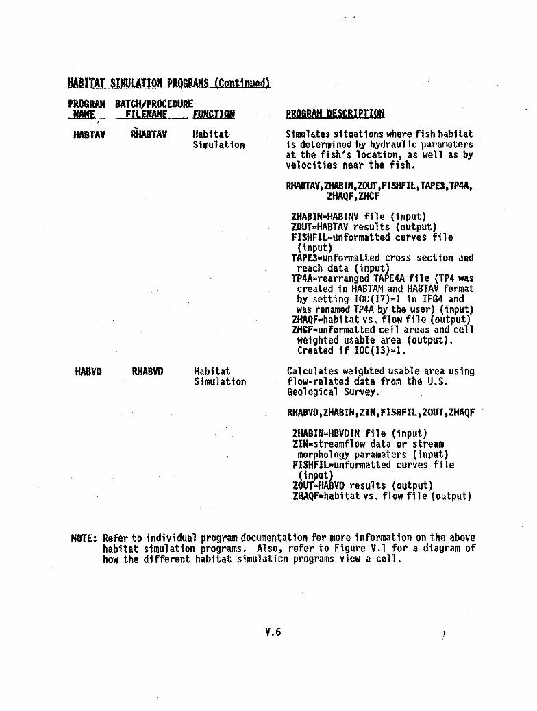
.IlW.IAI SIIIllAI.IDJJ PRQ&lWJS (Continued)
BATCH/PROCEDUREFuME FUNCTION
RHAsTAV HabitatSimulation
PROQRAMNAME
HABTAY
HABVD RHABVD HabitatSimulation
PROGRAM DESCRIPIION
Simulates situations where fish habitatis determined by hydraulic parametersat the fish's location, as well as byvelocities near the fish.
RHABTAV,ZHABIN,ZOUT,FISHFIL,TAPE3,TP4A,ZHAQF,ZHCF
ZHABIN-HABINV file (input)ZOUT-HABTAV results (output)FISHFIL-unformatted curves file(input)
TAPE3-unformatted cross section andreach data (input)
TP4A-rearranged TAPE4A file (TP4 wascreated In HABTAM and HABTAV formatby setting IOC(I7)-I in IFG4 andwas renamed TP4A by the user) (input)
ZHAQF-habitat vs. flow file (output)ZHCF-unformatted cell areas and cellweighted usable area (output).Created if IOC(I3)-1.
Calculates weighted usable area usingflow-related data from the U.S.Geological Survey.
RHABVD,ZHABIN,ZIN,FISHFIL,ZOUT,ZHAQF
ZHABIN-HBVDIN file (input)ZIN-streamf1ow data or streammorphology parameters (input)
FISHFIL-unformatted curves file(input)
ZOUT-HABVD results (output)ZHAQF-habltat vs. flow file (output)
NOTE: Refer to individual program documentation for more information on the abovehabitat simulation programs. Also, refer to Figure V.I for a diagram ofhow the different habitat simulation programs view a cell.
V.6 J

HABITAT SIMULATION -OPTIQHS FILE CREATION·ANQ MODIFICATION
PROGRAM BATCH/PROCEDURENAME FILENAME FUNCTION PROGRAM DESCRIPTIQH
HABIN RHABIN HAIlTAT Builds a HABTAT options file Which mayOptions File contain hydraulic data, cross sectionCreation data, or formatted FISHCRV type
data.
RHABIN,ZHABIN
ZHABIN-HABTAT options file (output)
HABINE RHABINE HABTAE Builds a HABTAE options file.Options FileCreation RHABItIE ,ZHADIN
ZHABIN-HABTAE options file (output)
HABINM RHABINM HABTAM Builds a H~BTAM options file.Options FileCreation RHABINM,ZHABIN
IHABIN-HABTAM options file (output)
HABINS RHABINS HABTAT Builds a HABTAT options file.Options FileCreation RHABINS,ZHABIN
ZHABIN=HABTAT options file (output)
HABINV RHABINV HABTAV Builds a HABTAV options file.Options FileCreation RHABINV,ZHABIN
lHABIN=HABTAV options file (output)
HBVOIN RHBVDIN HABVO Builds a HABVO options file.Options FileCreation RHBVDIN,ZHABIN
ZHABIN-HABVO options file (output)
V.l

HMmT SUlllJArnllf • OlIZDl!S..fILE CRWIDI.f MID HDDlFICATIOH (ContillllilU
BATCH/PROCEDUREFIlENA!!E FUNCTION
RMAKAVD AVDEPTHInput FileCreation
PROGIWINAME
MAKAVD
KODIOC MODIOC
PROGRAIJ DESCRIPTION
Creates an input file for the AYDEPTHprogram from a WSP or IFG4 data set;water surface elevations are read froma TAPE4 (generated from the input dataset) or entered interactively.
RMAKAVD,ZIN,ZAVJN,TAPE4
ZIN-IFG4 or WSP data set (input)ZAVJN-AVDEPTH data set (output)TAPE4-unforrnatted flow data (optionalinput)
IFG4/WSP/MANSQ/ Changes options in the selected dataHABTAT/HABTAM/ set or options file.HABTAV/HABTAE/HABVD Data Set RMODIOC.ZIN,IOUTModification
lIN-original data set (input)lOUT-new data set with modifiedoptions (output)
V.8

HABIlAT SIMULATION . MISCELLANEOUS
HQF2LT RHQF2LT
PROGRAMNAME
COlIfQF
BA~i=~EDURE. FUNCTION
RCOMHQF Habitat'. Simul ation ..Miscellaneous
HabitatSimulationMi sce11 aneous
PROGRAM DESCRIPTION
Averages or combines habitat area datafrom two habitat vs. streamflow filesbased on weighting factors suppliedby the user. The weight for the firstfile must be less than or equal to "1".The weight for the second file isassumed to be "I" minus the first fileweight. Any number of ZHAQF files maybe combined by adjusting the weightfactors and running COMHQF on two ZHAQFfiles at a time. .
RCOMHQF,ZHAQFN,ZHAQF,ZHAQF2,ZOUT
ZHAQFN-averaged or combined habitatarea versus streamflow file (output)
ZHAQF=habitat area vs. streamflowfile (input)
ZHAQF2=habitat area vs. streamflowfile (input)
ZOUT-averaged or combined habitat areain tables for each individual lifestage (output)
Converts a habitat vs. streamflow fileto a file that is readable by lOTUS.
RHQF2LT,ZHAQF,ZOUT
ZHAQF-habitat vs. flow file (input)ZOUT-LOTUS readable ZHAQF file(output)
SUMflQF RSIJIilHQF HabitatSimulation .Mi sce11 aneous
V.9
Sums conditional cover columns in aZHAQF file into one habitat vs. flowfigure for each life stage. Run whenconditional cover curves were used asinput to the habitat simulationprograms. Allows up to 5 life stagesto be grouped in each record.
RSUMHQF,ZHAQF,ZHAQFN
ZHAQF-habitat vs. streamflow file(input)
ZHAQFN=modified ZHAQF file withcolumns summed (output)
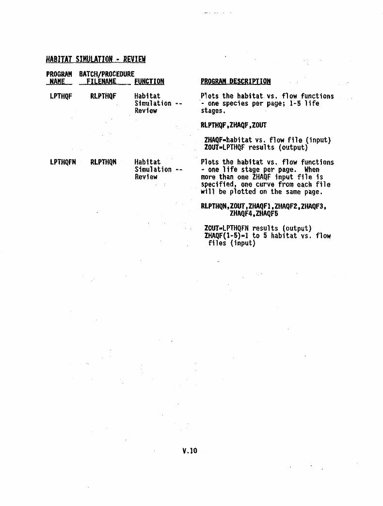
HABITAT SIMULATION • REVIEWPROGRAM BATCH/PROCEDURE
NAME FILENAME FUNCTION
LPTHQF RLPTHQF HabitatSimulation -Review
PROGRAM DESCRIPTION
Plots the habitat vs. flow functions- one species per page; l~S lifestages.
LPTHQFN RLPTHQN HabitatSimulation -Review
V.10
RlPTHQF.ZHAQF,ZOUT
ZHAQF-habitat vs. flow file (input)ZOUT-LPTHQF results (output)
Plots the habitat vs. flow functions- one life stage per page. Whenmore than one ZHAQF input file isspecified, one curve from each filewill be plotted on the same page.
RLPTHQN.ZOUT,ZHAQFl.ZHAQF2,ZHAQF3,ZHAQF4,ZHAQF5
ZOUT-LPTHQFN results (output)ZHAQF(l-S)-l to 5 habitat vs. flowfiles (input)

AVDEPTH and AVPERK programs
I. INTRODUCTION
Wetted perimeter, wetted width, and average velocity have long been usedas indexes to the physical habitat in a stream. In using the wetted width orwetted perimeter, the assumption is made that all the area of the stream is ofequal value to the instream flow activity of interest. The wetted perimeter andwetted width will always either stay the same or increase with depth. If these,and the above, assumptions can be made, then the use of the AVDEPTH and AVPERMprograms is appropriate.
The major difference between the AVDEPTH and the AVPERH programs is inputto the programs. The AVDEPTH program uses a WSP-type data set with at leasttwo additional lines added to the top. The first line contains controls for thecalculation and output for the AVDEPTH program; the other additional linescontain water surface elevations for the cross sections. The AVPE!lM program usesa TAPE3 which contains unformatted cross section and reach data. and a TAPE4which contains unformatted flow data. These two files are generated by thehydraulic simulation programs. In AVDEPTH, the weight on a cross section isalways 0.5; In AVPERM, the weight is written to the TAPE3 resulting from thehydraulic simulation process. PHABSIM programs assume that the hydraulicvariables measured at a cross section extend halfway to adjacent ·cross sectionsupstream and downstream. If this is not the case, upstream weighting factorsshould be applied.
The output resulting from AVDEPTH and AVPERM gives information for eachcross section and a summary of the average parameters for a whole reach of streamincluding discharge, depth, cross-sectional data, and velocity. fn addition,for each of the specified depths (maximum of five), AVDEPTH and AVPERH calculatethe total width of the stream that is as least as deep as the specified depth(Figure V.l).
The advantage of using the wetted width or wetted perimeter approach fordeveloping indexes to physical habitat in a stream is that the developmentrequires much less field and office work than the use of the weighted usable areaapproach used in PHABSIM. This savings in effort results from:
1. Species criteria not haVing to be developed or obtained;2. If using AVDEPTH, velocities need not be measured for the purpose of
calibrating a hydraulic simulation model to velocities, although thedischarge must be known; and
3. The interpretation of the results requires the use of only one factor(i.e., wetted perimeter or wetted Width) in contrast to the many possiblelife stages (factors) which may need to be considered when using weightedusable areas.
The use of wetted width is a special case of weighted usable area in whichthe weights are 1.0 for all velocities, depths, and channel indexes. Becausethe wetted perimeter is nearly the same as the wetted width, the same can be saidfor the wetted perimeter as well.
V.U Programs AVDEPTH and AVPERH
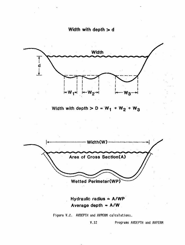
Width with depth > d
II II I"'" WrlO!
Width
II tI I.-... W3---lOo\
Width with depth> 0 '"' Wi + W2· + W3
1+'------Width(W)------.....·1
Area of Cross Section(A)
Wetted Perlmeter(WP)--
Hydraulic radius ,;" A/Wp·Average depth ... A/W
Figure V.2. AVDEPTH and AVPERM calculations.
V.12 Programs AVDEPTH and AVPERM
II. RUNNING AVDEPTH
The MAKAVD program is used to convert a NSP or IFG4 data set to an AVDEPTHdata set. Refer to Appen~ix Afor wAVDEPTH Data Set Formatn and information onwhat each line contains. Appendix A also contains a sample AVDEPTH data set.
RAVDPTH,ZAVIN,ZOUT,ZHAQF
ZAVIN=AVOEPTH data set (NSP type data set with control lineand water surface elevations .added to the top) (input)
ZOUT-AVOEPTH results (output)ZHAQF-habitat vs. flow file (output)
NOTE: On the microcomputer, graphs may be printed to the screen or to the outputfile using character graphics (132 characters per line format). In orderto use screen graphics, the computer must have a Color Graphics Adaptor(CGA) or compatible graphics card. When using screen graphics, notes arewritten to the output file in the positions where the graphs would havebeen placed had they been written using character graphics.
Appendix A contains the AVOEPTH dataset that was used to generate theoutput in Figure V.3. Figure V.4 contains the ZHAQF file created by AVDEPTH.
III. AVDEPTH ERROR MESSAGES
Most of the error messages result from data set format errors. Refer toAppendiX A for "AVOEPTH DataSet Format" and "WSP Data Set Format".
1. THERE IS II PROBLEM IN STATIONING OF TRANSECT NO•••• OR TRANSECT NO. --THE TWO NUMBERS APPEAR ON LINES THAT ARE RIGHT NEXT TO EACH OTHER IN THEDATA FILE.
The program will use the first station number and continue to run.
V.IS Program AVDEPTH

88/07/26.11.52.45.
UPPER SALllOIf RIVER. HEAR STMLEY. lOAllOAVDEPTH MfA 5ET CREATfD FR(lII AN IFG4 DATA SET WITH THE MMAVD PROGRAM
PROGRAM-AVDEPTHPAGE- 2
ONLY THE DATA FOR CROSS SECTION 0.00 HAS BEEN INCLUDEO IN THIS SAMPLE OUTPUT.
COORDINATE DATA FOR CROSS SECTlOll 0.00
015TMCE 0.00 2.50 4.00 4.30 5;SO 7.60 11.90 14.20 16.20 16.50ELEVATlOlI 101.30 100.70 99.80 98.50 97.70 97.30 97.60 97.90 97.60 97.70
DISTMCE 18.20 20.20 22.20 24.20 26.20 28.20 3UO 32.20 33.00 34.20ELEVATION 97.50 97.40 97.30 97.20 97.30 97.60 97.40 97.70 97.60 97.60
DISTANCE 35.20 36.20 37.40 39.10 43.80 53.00 62.40 69.90 78.10 87.10ELEVATION 97.70 97.70 97.70 97.90 98.10 98.80 99.00 98.50 99.00 99.50
ESTIMATE OF PARAMETERS FOIl CROSS SECTION 0.00
WATER CHANNEL SURFACE AVERAGE WETTED HYDRAUliC FLOW SURFACEWIOfK WITH DEPTH OF AT lEASTELEVATION AREA WIDTH DEPTH PERIHEfER RADIUS FACTDR 0.25 FT 0.50 FT 1.00 FT 1.50 FT 2.00 FT FLOw VELOCITY
97.68 5.84 25.72 0.23 25.85 0.23 3.6972 11.25 0.00 0.00 0.00 0.00 8.00 1.37
97.72 6.95 29.52 0.24 29.57 0.23 3.7893 14.30 0.80 0.00 0.00 0.00 10.00 1.44
97.84 10.68 32.42 0.33 32.84 0.33 3.9540 19.71 5.98 0.00 0.00 0.00 20.00 1.88
97.93 13.68 34.61 0.40 34.87 0.39 4.0930 25.72 11.25 0.00 0.00 0.00 30.00 2.19
98.01 18.53 36.80 0.45 36.89 0.45 4.1335 30.48 16.93 0.00 0.00 0.00 40.00 2.42
98.08 19.15 38.34 0.50 38.65 0.50 4.1701 3U8 19.38 0.00 0.00 0.00 50.00 2.61
98.13 21.10 39.43 0.54 39.76 0.53 4.3398 33.38 22.93 0.00 0.00 0.00 60.00 2.84
98.19 23.50 40.61 0.56 40.97 0.57 4.3155 34.85 26.28 0.00 0.00 0.00 70.00 2'98
98.23 25.14 41.40 0.51 41.71 0.80 4.4549 35.85 29.76 1.20 0.00 0.00 80.00 3.18
98.28 27.23 42.39 0.64 42.77 0.54 4.4659 37 ..09 30.91 3.20 0.00 0.00 90.00 3.31
98.32 28.94 43.l7 0.67 43.58 D.55 4.5389 38.09 31.93 4.99 0.00 0.00 100.00 3.46
98.36 30.89 43.96 0.70 44.38 0.89 4.5841 39.03 32.90 6.97 0.00 0.00 110.00 3.58
98.40 32.48 44.75 0.73 45.18 0.12 4.6090 39.62 33.81 8.98 0.00 0.00 120.00 3.70
98.44 34.27 45.54 0.15 45.99 0.75 4.5161 40.61 4.86 12.01 0.00 0.00 130.00 3.79
Figure V.3. Sample output from the AVOEPTH program.
V.14 Program AVDEPTH.

fBIIff(l6. lfI'Ill SAIJOl RIVER, _ STNUY. IlWD _·A\lIEP11I11.52.46. A\lIEP11I MTA SEf QlfATB> FRlM Nl 1fG/i MfA SEf 1II1ll TIE__ PIlE· 3
102.00 , 1 1 1 1 1 1 1 1 I ,, 1 1 1 I 1 1 1 1 I ,, 1 1 1 1 1 1 t 1 1 ,, ,lilt .50 1/- ••• .. ~ ..,, •
* •• •, •101.00 11- ••• •••••, •• •• * •• •too.50 11-... .....• •, •• •• •100.00 •.... ....., •• * •ElEVATll)l • •, •99.500 11-... ~"'K~', •, ,• •• •99.00l ..... • • ....•f •, •, •, • •CJIl.5OO ..... • ....., •• •• ff • •CJIl.OOl 11- ... ....., • • •, ,f • • .... •, * • .. ,
97.500 ,.... • • ....f, • • f
• • 1 1 • ., 1 1 1 1 t I ,II 1 1 * 1 I 1 1 1 1 1 IIII 1 1 t t t 1 1 1 1 ,
97.00lO.ll:XXXl1·ot 18.00l 36.00l 54.00l 72.00l 'lO.00l
OOסס.9 27.000 45.000 63.000 81.00l
OISTNlE
llQl$ sa:rl()l 0.00
Figure V·.3. (Continued)
V.15 Program AVDEPTH

88/07126.11.52.46.
UPPER SAlMON RIVEll. NEAR STMlEY, IDAriOAVDEPTH DATA SET CREATED FROM AN IF64 DATA SET IIITH THE MAKAVD PROGRAM
PROGRAM-AVOEPTHPAGE- 6
SUMMARY OF AVERAGE PARAMETERS FOR \/HOlE REACH
IIETtED IIIDTH IIITH DEPTH GREATER THANDISCHARGE PEllIMETER 1I10TH 0.25 0.50 l.OD 1.50 2.00 DEPTH CIS AREA VELOCITY
8.00 23.73 23.63 13.77 0.00 0.00 0.00 0.00 0.27 6.3 1.2610.00 25.98 25.86 16.42 0.40 0.00 0.00 0.00 0.28 7.3 l.3720.00 30.45 30.29 20.13 8.69 0.00 0.00 0.00 0.36 10.9 1.6430.00 32.75 32.57 23.88 14.80 0.00 0.00 0.00 0.42 13.8 2.1740.00 34.71 34.50 26.93 18.37 0.00 0.00 0.00 0.48 16.5 2.4250.00 39.35 39.12 30.17 19.96 0.00 0.00 0.00 0.49 19.1 2.6260.00 42.09 41.85 31.48 22.15 0.00 0.00 0.00 0.51 21.3 2.8170.00 43.66 43.40 32.61 24.24 0.00 0.00 0.00 0.55 23.7 2.9680.00 44.63 44.56 33.77 26.31 3.20 0.00 0.00 0.57 25.4 3.1590.00 46.10 45.82 35.28 27.25 5.40 0.00 0.00 0.60 27.4 3.28
100.00 47.27 46.97 37.93 28.07 7.50 0.00 0.00 0.82 29.3 3.41110.00 48.25 47.94 40.01 30.65 9.54 0.00 0.00 0.85 30.9 . 3.56120.00 49.42 49.10 41.85 31.61 11.93 0.00 0.00 0.67 32.9 3.65130.00 50.40 50.07 42.82 32.46 14.50 0.00 0.00 0.69 34.6 3.76
HORMAl END OF JOB
Figure V.3. (Concluded)
V.16 Program AVOEPTH

'.
UPPER SAlMON RIVER, NEAR STAHLEY, IDAHOZHAQF FILE GENERATED 8Y TliE AVDEPTH PROGRAI1WIDTH AND WETTED PERIHETER
DISCHARGE WIDTH WETTED P* 1 8.00 23.83 23.73* 2 10.00 25.88 25.98* 3 20,00 30.29 30.45* 4 30.00 32.57 32.75* 5 40.00 34.50 34.71* 6 50.00 39.12 39.35* 7 80.00 41.85 42.09* 8 70.00 43.40 43.65• 9 80.00 44.56 44.83*10 90.00 45.82 46.10*11 100.00 46.97 47.27*12 110.00 47.94 48.25***************
X' 0.50 X' 1.00 X= 1.50 X· 2.000.00 0.00 0.00 0.000.40 0.00 0.00 0.008.69 0.00 0.00 0.00
14.80 0.00 0.00 0.0018.37 0.00 0.00 0.0019.96 0.00 0.00 0.0022.15 0.00 0.00 0.0024.24 0.00 0.00 0.0025.31 3.20 0.00 0.0027.25 5.40 0.00 0.0028.07 7.50 0.00 0.0030.65 9.54 0.00 0.00
WIDTH WITH DEPTH GREATER THAN XDISCHARGE X= 0.25
11 1 8.00 13.77• 2 10.00 16,42* 3 20.00. 20.13• 4 30.00 23.88* 5 40.00 26.93• 6 50.00 30.17* 7 60.00 31.48• 8 70.00 32.81* 9 80.00 33.77'10 90.00 35.28'11 100.00 37.93*12 1I0.00 40.01***************CROSS SECTIONAL AREA
DISCHARGE CIS AREA, 1 8.00 6.33* 2 10.00 7.32, 3 20.00 . 10.85* 4 30.00 13.83* 5 40.00 18.51• 6 50.00 19.09* 7 80.00 21.34, 8 70.00 23.67, 9 80.00 25.43'10 90.00 27.44'11 100.00 29.30'12 110.00 30.94***************HEAN CHANNEL VELOCITY
DISCHARGE, 1 8.00, 2 10.00, 3 20.00* 4 30.00• 5 40.00* 6 50.00* 7 60.00, 8 70.00, 9 80.00'10 90.00*11 100.00*12 !l0.00*******-******
VELOCITY .1.261.371.842.172.422.622.812.963.153.283.413.55
Figure V.4. ZHAQF file generated by AVDEPTH.
V.17 Program AVDEPTH

IV. RUNNING AVPERMRAVPERH,ZOUT.TAPE3,TAPE4.ZHAQF
ZOUT-AVPERH results (output)TAPE3=unformatted cross section and reach data (input)TAPE4=unformatted flow data (input)ZHAQF=habitat vs. flow file (output)
ENTER NUMBER OF DEPTHS (5 MAX):
If depths are specified. the AVPERH program will calculate the total widthof the stream that is as least as deep as the depth(s) specified.
ENTER THE --- DEPTHS:
Figure V.5 contains sample output from the ZOUT file created by AVPERH.Figure V.S contains the ZHAQF file generated by AVPERH.
V.IS Program AVPERH

MTE - 88/10/04. lJf>PER SALMON RIVER, NEAR STANLEY, IDANO PROGRAM • AVPERHTI~ . 13.12.34. IFG4 DATA SET VITH VS. LINES ADDED FROM MANSQ PAGE· 1
AVERAGE PARAMETERS FOR CROSS SECTION 0.00
V.S. AVERAGE HYDRAULIC HYORAULIC VETTED If<TTEO mOUDE DRAG WADINGDISClll\RGE ELEV VELOCITY DEPTH RADIUS WIOTH PERIMETER NUM8ER PARAMETER PARAMETER CIS AREA
8.0 97.68 1.37 o.n 0.23 25.7 25.9 0.51 0.43 0.31 5.810.0 97.72 1.44 0.24 0.Z3 29.5 29.7 0;52 0.49 0.34 6.920.0 97.84 1.88 0.33 0.33 32.4 32.6 0.58 1.18 0.62 10.730.0 97.93 2.19 0.40 0.39 34.6 34.9 0.61 1.90 0.87 13.740.0 98.01 2.42 0.45 0.45 36.6 36.9 0.63 2.65 1.09 18.550.0 98.08 2.61 0.50 0.50 . 38.3 38.7 0.85 3.41 1.30 19.260.0 98.13 2.84 . 0.64 0.53 39.4 39.8 0.69 4.33 1.5Z 21.170.0 98.19 2.98 0.58 0.57 40.6 41.0 0.69 5.14 1.72 23.580.0 98.23 3.18 0.81 0.60 41.4 41.8 0.72 6.15 1.93 25.190.0 98.28 3.31 0.64 0.84 42.4 42.6 0.73 7.02 2.12 27.2
100.0 98.32 3.48 0.67 0.88 43.2 43.5 0.74 8.00 2.32 28.9110.0 98.38 3.58 0.70 0.68 44.0 44.4 0.76 8.97 2.50 30.1120.0 98.40 3.70 0.73 0.72 44.8 45.2 0.75 9.91 2.68 32.5130.0 98.44 3.79 0.75 0.75 45.5 46.0 0.17 10.83 2.85 34.3
ORAG PARAHETER • (VELOCITY" 2.01 • DEPTHVADING PARAIIETER • VELOCITY • DEPTH
OEPTH PARAMETERS FOR CROSS SECTION 0.00
TOTAL VIDTH WITH DEPTH GREATER THANDISCHARGE WIDTH 0.25 0.50 1.00 1.50 2.00
SUM CONT. W SUM CONT. W SUM CONT. W SUM CONT. W SUM CONT. 1/
8.0 26. 11. 8. O. O. O. O. o. O. O. O.10.0 30. 14. 9. 1. 1. O. O. O. O. O. O.20.0 32. 20. 14. 6. 5. O. O. o. o. o. O.30.0 35. 26. 15. 11. 8. O. O. o. O. O. O.40.0 31. 30. 23. 11. 13. O. O. O. o. o. O.50.0 38. 32. 24. 19. 14. O. O. O. o. o. O.60.0 39. 33. 25. 23. 15. O. O. o. O. O. O.70.0 4l. 35. 35. 28. 18. O. . O. o. O. O. D.80.0 41. 38. 38. 30. 22. l. 1. O. O. O. D.90.0 42. 37. 37. 31. 23. 3. 3. O. O. o. O.
100.0 43. 38. 38. 32. 24. 5. 5. O. O. o. O.110.0 44. 39. 39. 33. 24. 7. 6. O. O. o. O.120.0 45. 40. 40. 34. 34. 9. 1. O. O. O. O.130.0 46. 41. 4l. 35. 35. lZ. 8. O. O. O. O.
wCONT. 11" 15 MAXIMUM CONTIGUOUS WIOTH
ONLY THE INFORMATION FOR THE FIRST CROSS SECTION IS INCLUDED IN THIS SAMPLEOUTPUT.
Figure V.S. Sample output from the AVPERM program.
V.19 Program AVPERM

DATE - 66/10/04. UPPER SAlMON RIVER. NEAR STANLEY. IDAHO PROGRAM - AVPERMTIME - 13.12.34. IFG4 DATA SET WITH WSL LIMES ADDEO FROM IIAHSQ PAGE - 3
SUMMARY OF AVERAGE PARAMETERS FOR WHOLE REACH
WETTeD WIDTH WITH DEPTH GREATER THANDISCHARGE PERIMETER WIDTH 0.2S 0.50 I. DO 1.50 2.00 DEPTH CiS AREA VELOCITY
6.00 22.66 -22.79 14.76 0.00 0.00 0.00 0.00 0.29 6.5 l.23
10.00 24.50 24.40 17.27 0.24 0.00 0.00 0.00 0.31 7.5 1.34
20.00 29.56 29.44 20.30 9.76 0.00 0.00 0.00 0.37 10.9 1.63
30.00 31.90 31.75 23.14 1(>'23 0.00 0.00 0.00 0.44 13.9 2.16
40.00 33.83 33.66 25.50 18.94 0.00 0.00 0.00 0.49 16.5 2.42
50.00 39.63 39.44 29.37 20.19 0.00 0.00 0.00 0.48 19.1 2.62
60.00 43.02 42.62 30.72 21.64 0.00 0.00 0.00 0.50 21.4 2.60
70.00 44.73 44.51 31.99 23.42 0.00 0.00 0.00 0.53 23.7 2.95
60.00 46.05 45.62 32.94 24.93 4.00 0.00 0.00 0.56 25.5 3.13
90.00 47.43 47.19 34.56 25.76 6.26 0.00 O.DO 0.56 27.5 3.27
100.00 46.75 46.49 37.66 26.52 6.50 0.00 0.00 0.61 29.4 3.40
110.00 49.60 49.54 40.40 29.75 10.56 0.00 0.00 0.63 31.0 3.54
120.00 51.12 50.64 42.67 30.70 13.12 0.00 0.00 0.65 33.1 3.63
130.00 52.17 51.66 43.71 31.49 15.50 0.00 0.00 0.67 34.7 3.74
Figure V.S. (Concluded)
V.20 Program AVPERM

UPPER SALMON RIVER, HEAR STAHLEY, IDAHOZHAQF FILE CREATED BY THE AVPERM PROGRAMWIDTH AMO WETTED PERIMETER
DISCHARGE WIDTH WETTED P* 1 6.00 22.79 22.88* 2 10.00 24.40 24.511* 3 20.00 29.44 29.58* 4 30.00 31.75 31.90" 5 40.00 33.66 33.83w 6 50.00 39.44 39.63* 7 60.00 42.82 43.OZ" 8 70:00 44:51 44.73* 9 80.00 45.82 46.05"10 90.00 47.19 47.43"11 100.00 48.49 48.75*12 110.00 49.54 49.80********"''''*'ltit'lrltWIDTH WITH DEPTH GREATER THAM X
DISCHARGE X. 0.25 XW 0.50 X· 1.00* I 8.00 14.76 0.00 0.00* 2 10.00 17.27 0.24 0.00* 3 20.00 20.30 9.78 0.00* 4 30.00 23.14 16.23 0.00* 5 40.00 25.50 18.94 0.00* 6 50.00 29.37 20.19 0.00* 7 60.00 30.72 l1.84 0.00* 8 70.00 31.99 23.42 0.00*9 80.00 32.94 24.93 4.00*10 90.00 34.56 25.76 6.28*11 100.00 37.86 26.52 8.50*12 110.00 40.40 29.75 10.56***.*'**********CROSS SECTIOHAl AREA
DISCHARGE CIS AREA* 1 8.00 6.53* 2 10.00 7.47* 3 20.00 10.93* 4 30.00 13.66• 5 40.00 16.50• 6 50.00 19.06* 7 60.00 21.43* 8 70.00 23.74* 9 60.00 25.54*10 90.00 27.53*11 100.00 19A4"12 110.00 31.04****"'***Il*****.MEAN CHANNEL VELOCITY
DISCHARGE VELOCITY* 1 8.00 l.23" 2 10.00 1.34* 3 20.00 1.63* 4 30.00 2.16* 5 40.00 2.42" 6 5ll.00 2.62* 7 60.00 2.60* 8 70.00 2.95* 9 80.00 3.13*10 90.00 3.27*11 100.00 3.40*12 llO.OO 3.54******ft********
X' 1.500.000.000.000.000.000.000.000.000.000.000.000.00
x- 2~OO
0.000.000.000.000.000.000.000.000.000.000.000.00
Figure V.6. ZHAQF file generated by AVPERM.
V.Zl Program AVPERM

C_F ProgramI. INTRODUCTION
The COMHQF frogram averages or combines habitat area data. from two habitatvs. streamflow fi es based on weighting factors supplied by the user. The weightfor the first file must be less than or equal to *1*. The weight for the secondfile is assumed to be *1* minus the first file weight. Any number of ZHAQF filesmay be combined by adjusting the weight factors and running COMHQF with each setof two files.
The equation used when combining two files with weights is:
HAC - (HAl x WI) + (HA2 x W2)W2 - 1.0 - WIWI s 1.0QI - Q2
where HAl - habitat area from the first ZHAQF fileHA2 - habitat area from the second ZHAQF fileHAC - combined habitat area
WI =weight on first ZHAQF fileW2 =weight on second ZHAQF fileQl - streamflow from first ZHAQF file, andQ2 - streamflow from second ZHAQF file
II. RUNNING COMHQF
RCOMHQF,ZHAQFN,ZHAQF,ZHAQF2,ZOUT
ZHAQFN-averaged or combined habitat vs. flow file (output)ZHAQF-habitat vs. flow file (input)ZHAQF2-habitat vs. flow file (input)ZOUT-averaged or combined habitat area in tablesfor each individual life stage (output)
The two title lines from the two input files are displayed.
ENTER TWO LINE TITLE
These· two title lines will be in the averaged or combined output file.
If the *life Stage Lines* are not the same on both ZHAQF files specified asinput, the follOWing message will appear, but the program will not abort:
WARNING - LIFE STAGE TITlES 00 HOT MATCH.WIll USE LIFE STAGE TITLE FROM FIRSTHAQF FIlE
V.22 Program COMHQF

- ....• --- -- ,- --- ... _- -_._-- --.-
Input files need to be in the same format and contain the same type ofinformation to be logically combined, i.e., combining different habitatsimulation figures for the same discharges, species, and life stages offish would be logical.
ENTER 0 TO AVERAGE HAQF FILES,1 TO COMBINE WITH WEIGHTS:
If "I" is entered to combine with weights:
ENTER WEIGHT FOR FLOWS ON SET 1
ENTER WEIGHT FOR WUA ON SET 1 -
The weights for the first file must be less than or equal to "I".The weight for the second file is assumed to be "1" minus the firstfil e weight.
V.23 Program COMHQF
HABIN ProgrlllR
I. INTRODUCTION
The HABIN program builds the long form of a HABTAT options file which maycontain hydraulic data, cross section data, or formatted FISHCRV type data.This file is used as input to the HARTAT program.
It is recommended that the HABINS program be used to create the HABTAToptions file versus using the HABIN program.
Refer to Appendix A, HABTAT Options File Format, for file format for aHABIN file.
II. RUNNING HABIN
RHABIN,ZHABIN
ZHABIN=HABTAT options file (output)
DO YOU WISH TO:(1) GENERATE A COMPLETE DATA SET,(2) GENERATE DATA UP TO CURVE SETS,(3) GENERATE JUST FLOW DATA,(4) GENERATE JUST CURVE SETS, OR(5) GENERATE IDe, HEADER, AND CURVES LINES ONLY.
1 = The IOC, TITLE, HEADER, and CURVES lines are entered into the options filealong with the criteria curves data, cross section data, and hydraulicdata. No previously created files are utilized as input to HABTAT.
2 = The 10C. TITLE. HEADER, and CURVES lines are entered into the options filealong with the cross section and hydraulic data. A previously createdFISHFIL is also used as input to HABTAT.
3 = The file resulting from this option cannot be used as input to HABTAT inplace of a TP4. In order to read flow data from the options file, thecross section data must also be read from the options file (IOC(8)=0).Therefore, if flow data is to be entered into the options file, selectOption I or 2 above.
4 = Just the Hline and POINT lines of the criteria curve data are written toa file. In order to utilize this file, it would have to be appended tothe end of the file created' by selecting Option 5 in HABIN, or appendedto the bottom of the HABTAT options file created by the HABINS program.It is recommended that the criteria curve data be entered using the GCURVprogram to create a FISHCRV file. This file could either be convertedto a FISHFIL and used as input to HABTAT or, it could be appended to thebottom of the HABTAT options file created by HABINS (remove the titleline).
5: This option is the same as running the HABINS program.
V.24 Program HABIN

Figure V.7 contains a sample direct entry HABTAT input file created by theHABIN program.
IOC 1'11001ODDI0ODDOOOOOOOOOOOaDOOaDaDOOOOaDOEXAIlPLE 01' A DIRECT ENTRY HABTAT INPIJT FILE CREATED BY HABINDATA FRDN THE SANPLE IFG4 DATA SET IS INCLUDED IH THIS FILEHEADER IcUtVES -21112XHEAD 0.0 3D 14.25 0.30COORD 0.0 D.aD 101.30 2.50 100,70 4.00 99.80COORD 0.0 4.30 98.60 5.50 97.70 7.80 97,30COORD 0.0 11.90 97.60 14,20 97,90 16,20 97.60COORD 0,0 16.50 97.10 18.20 97.50 20.20 91.40COORD 0.0 22.20 97.30 24.Z0 97.20 26.20 97.30COORD 0.0 28.20 97.50 30.20 91.40 32.20 97.70COORD 0.0 33.00 97.60 34,20 97.60 35.20 97.70COORD 0.0 36.20 97,70 37,40 97.70 39,10 97.90COORD 0.0 43.80 98,10 53.00 98.60 62.40 99.00COORD 0.0 69,90 98.50 78,10 99.00 81.10 99.50SUBSTR 0.0 3.0 3.0 3.0 3.0 9.2 6.0 6.0 8.2 8.2 8.2 8.2 9.0SU8STR 0.0 9.0 9.0 9.0 9.0 9.0 9.0 9.0 9.2 9.2 9.2 9.2 10.0SUBSTR 0.0 10.0 10.0 10.0 8.2 3.0 3.0XHEAO 14.3 32 0.00 0,50COORD 14.3 0.00 101.90 3.00 101.30 4.70 101.00COORD 14.3 5.30 100.00 15.00 100,00 19.10 99.60COORD 14.3 29.30 99.20 33.10 98.40 41.00 68.50COORD 14.3 46.10 98.20 48.10 98.00 48.50 97.90COORD 14.3 49.30 97.80 50.30 97.80 52.30 97.70COORD 14.3 54.20 97.60 58.30 97.80 58.30 97.60COORD 14.3 60.30 97.60 62.30 91.60 64.30 97.70COORD 14.3 65.00 97.80 66.30 97.70 68.30 97.90COORD 14.3 70.30 98.20 73.80 98,20 77.70 98.80COORD 14.3 86,60 99.00 94.30 96.50 99.10 98.90COORD 14.3 103.60 , laD. 30 108,40 101.305UBSTIl 14.3 3:0 3.0 3.0 3.0 3.0 3.0 3.0 3.0 7.4 8.2 8.5 8.5SUBsTR 14.3 8.0 0.5 9.2 9.0 9.0 9.0 9.0 10.0 10.0 9.0 9.0 10.0SUBSTR 14.3 10.0 10.0 10.0 10.0 10.2 9.5 7.7 3.0EHOXSECQHEAO 0.0 21.80 1 29 97.86VELOCI 0,0 0.0 0.0 0.0 0.2 0.2 0,0 0.0 0.0 0.3 1.3 2.4 2.3VELOCI 0.0 2.4 3.0 2.8 2.2 2.1 2.1 1.3 0.5 0.8 0.6 0.0 0.0VELOCI 0.0 0.0 0.0 0.0 0.0 0,0QHEAO 14.3 21.80 1 31 96.24VElOCI 14.3 0.0 0.0 0.0 0.0 0.0 0.0 0.0 0.0 0.0 0.4 0.9 1.5VElOCI 14,3 2.0 2.0 2,0 2.2 2.3 2.3 2.5 2.5 2.3 1.3 0.7 0.8VElOCI 14,3 0.3 0.0 0.0 0.0 0.0 0.0 0,0EHDQH 21112 4 8 8 o RAINIlOII TIlOUT FRYV 21112 0.00 1.00 0.10 1.00 0.50 0.00100.00 0.000 21112 0.00 0.00 0.10 0.10 0,20 1.00 0.50 1.00 1.00 0,50 1.25 0.300 21112 3.00 0.00100.00 0.00S 21112 0.00 LaD 1.00 1.00 2.00 1.00 4.00 1.00 6.00 1.00 Uo 1.00S 21112 9.00 1.00100.00 0.00
Figure V.7. Sample direct entry HABTAT input file created with HABIN.
V.25 Program HABIN

HABINE Program
I. INTRODUCTION
The MABINE program builds a MABTAE options file. The following files areused along with the HABINE options file as input to MABTAE: (1) a FISHFILcontaining criteria curves of aquatic species or recreational activities createdby the curve maintenance programs, (2) TAPE3 containing cross section data whichis output from IFG4 or WSP, and (3) TAPE4 containing hydraulic data which isoutput from IFG4 or WSP. BQti that HABTAE uses a TAPE4 as input versus a TP4as the other habitat simulation programs use. Also, the TAPE4 may have the cellvelocities calculated (as per HABTAT) or have velocities calculated at thecoordinate points (as per HABTAV and HABTAM).
Refer to Appendix A, HABTAE Options File Format, for file format for aHABINE file. Figure v.a contains a sample HABTAEinput file created by theHABINE program.
II. RUNNING HABINE
RHABINE.ZHABIN
ZHABIN=HABTAE options file (output)
The options are displayed and the user is asked to enter the IOC values.Typical settings for IOC values are O=OFF and I=ON. HABTAE options are describedin Table V.I in the HABTAE program documentation.
The following promots will appear in the following circumstances:
If IOC(14)=I
ENTER NOSE DEPTH:ENTER AAND B IN VNOSE = A*VMEAN**B:
If IOC(I4)=2
ENTER NOSE DEPTH:
If IOC(14H
ENTER NOSE DEPTH:ENTER 065 OF BED MATERIAL:
If IOC(14)=4
ENTER NOSE DEPTH:ENTER MANNING'S ROUGHNESS:
V.26 Program MABINE

If IOC{14}aS
ENTER NOSE DEPTH:ENTER AAND B IN VNOSE • A*VHEAN**B:
If IOC{l4)-6
ENTER NOSE DEPTH:ENTER MANNING'S ROUGHNESS:
If IOC(14)-7
ENTER HANNING'S ROUGHNESS:
If IOC{17)"3
ENTER 065 OF BED MATERIAL:ENTER SPECIFIC GRAVITY:
If IOC(16)-Zor 3
ENTER DEPTH OF CEll AT TOP OF WATER COLUMN:
HOW MANY CURVE SETS (MAX 40):
ENTER THE -- CURVE SET 10 NUMBERS (USUALLY 6 DIGIT):WHERE --
NEGATIVE NUMBERS INDICATE CURVE SETS ARE INCLUDED IN THIS FILE.POSITIVE NUMBERS INDICATE CURVE SETS WILL BE READ FROM AFISHFIl.
If IOC(ll)-1
ENTER MINIMUM CONTIGUOUS WIDTH FOR --- CURVES:
If IOC(19H
ENTER MINIMUM COMPOSITE SUITABILITY FACTOR:
If IOC(19)-2
ENTER MINIMUM COMPOSITE SUITABILITY FACTORS FOR --- CURVES:
V.27 Program MABINE

If 1OC(21)zl
ENTER VALUE OF IOC14 FOR _.- CURVES:
If the IOC14 value entered here is greater than zero, then theCurve ID number will be displayed and then the following prompt:
CURVE 10: -<.ENTER ICF PARAMETER:
The appropriate prompts for IOCI4, IOCI6. and IOC17 willbe asked depending on what the [CF parameter is set to.
[f 1OC(21)=2
ENTER VALUE OF IOC14 FOR ALL CURVES:ENTER ICF PARAMETER FOR ALL CURVES:
The appropriate prompts for [OCI4, IOCI6, and IOC17 will beasked depending on what the IeF parameter is set to.
IOC 011000000010000000001HfAOER 18CURVES -721001 720701 720702 720704 720601 720602 720603 720501 720502CURVES 720503 720202 720401 720403 720300 720302 720303 720904 720905Iol'tIH .00 .00 .00 .00 .00 .00 .00 10.00 15.00Iol'tIH .00 .00 20.00 10.00 15.00 15.00 10.00 5.00 5.00IHOSE 609900000000000099ONOSE 0 721001 .00 .035 .00OHOSE 4 720702 .00 ,00 .00OHOSE 4 720704 .00 .00 .00OHOSE 7 720904 .00 .00 .00OHOSE 7 720905 .00 .00 .00H 721001 6 4 4 o FISHIHG < BANK FLOAT-lUREV 721001 .00 .00 2.00 l.00 G.OO 1.00 9.00 .00 10.00 .00100.00 .00o 721001 .00 1.00 4.00 1.00 10.00 1.00100.00 l.00S 721001 .00 1.00 2.00 1.00 8.00 1.00100.00 1.00
Figure v.a. Sample HABTAE options file created with HABINE.
Criteria curves have been added to the end of this file. They can eitherbe added with an editor or created with GCURV and appended to the end of thisfile (if GCURV is used, delete the TITLE line). These curve sets are thenaccessed by entering curve set 10 numbers as negative numbers on the Curves line.Be sure to update the number of curves on the Header line if additional curveset ID numbers are added to the Curves line. Refer to Appendix A. "File Formatfor HABTAE Options File· CURVES Line" for more information.
The program adds zeros to the end of the IOC line to allow for futureoptions in the HABTAE program.
V.2a Program HABINE
HABINM Program
I. INTRODUCTION
The HABINM program builds a HABTAM options file. The following files areused along with the HABINM options file as input to HABTAM: (1) a FlSHFILcontaining criteria curves of aquatic species or recreational activities createdby the curve maintenance prQgrams, (2) TAPE3 containing cross section data whichis output from IFG4, and (3) TP4A containing hydraulic data which is output fromIFG4. TP4A is a TP4 created with IOC(17)=1 in the IFG4 program and then renamedTP4A by the user. This version of TP4 is in HABTAM and HABTAV readable fQrmatrather than HABTAT readable format.
Refer to Appendix A, HABTAM Options File Format, for file format forcreating a HABINM file. Figure V.9 contains a sample HABTAM input file createdby the HABINM program.
II. RUNNING HABINM
RHABIHM.ZHABIN
ZHABIN=HABTAM options file (output)
The options are displayed and the user is asked tQ enter the IOC values.Typical settings for IOC values are O=OFF and I=ON. HABTAM Qptions are describedin Table V.2 in the HABTAM program documentation.
The following prompts will appear in the following circumstances:
If IOC(6)=1 or IOC(14)=1
ENTER NOSE DEPTH:ENTER AAND B IN VNOSE = A*VMEAN**B:
If IOC(6)=2 or IOC(14)=2
ENTER NOSE DEPTH:
If IOC(6)=3 or IOC(14)=3
ENTER NOSE DEPTH:ENTER 065 OF BED MATERIAL:
HOW MANY CURVE SETS (MAX 40):
ENTER NUMBER OF FLOW PAIRS FOR MIGRATION CALCULATION:
ENTER NUMBER OF ADDITIONAL MIGRATION (ADMG) LINES:
V.29 Program HABINM
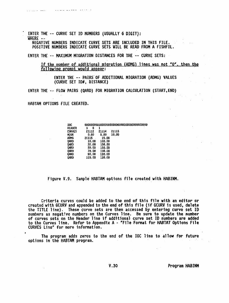
ENTER THE -- CURVE SET 10 NUMBERS (USUALLY 6 DIGIT):WHERE --
NEGATIVE NUMBERS INDICATE CURVE SETS ARE INCLUDED IN THIS FILE.POSITIVE NUMBERS INDICATE CURVE SETS WILL BE READ FROM A FISHFIL.
ENTER THE -- MAXIMUM MIGRATION DISTANCES FOR THE -- CURVE SETS:
If the number of additional migration (AQMG) lines was not ·0·. then thefollowing prompt would appear:
ENTER THE -- PAIRS" OF ADDITIONAL MIGRATION (ADMG) VALUES(CURVE SET 10#, DISTANCE)
ENTER THE -- FLOW PAIRS (QARD) FOR MIGRATION CALCULATION (START,END)
HABTAM OPTIONS FILE CREATED.
ICC 0000000001000000000000000000000000000000HEAOER 3 6 1tURVES 21112 2111~ 21115MIGR 0.00 5.00 10.00ADMG 21115 15.00QAAO 10.00 130.00QARO 30.00 130.00QARO 50.00 130.00QARO 70.00 130.00QARO 90.00 130.00QARD 110.00 130.00
Figure v.g. Sample HABTAM options file created with HABINM.
Criteria curves could be added to the end of this file with an editor orcreated with GCURV and appended to the end of this file (if GCURV is used, deletethe TITLE line). These ~urve sets are then accessed by entering curve set 10numbers as negative numbers on the Curves line. Be sure to update the numberof curves sets on the Header line If additional curve set 10 numbers are addedto the Curves line. Refer to Appendix A- ·Flle Format for HABTAT Options FileCURVES Line" for more information.
The program adds zeros to the end of the IOC 1ine to allow for futureoptions in the HABTAH program.
V.30 Program HABINH
WINS Prograll
1. INTRODUCTION
The HABINS program builds a HABTAT options file. This is the recommendedprogram, (vs. HABIN) for creating a HABTAT options file. The following filesare used along with this version of the HABTAT options file as input to HABTAT:(1) a FISHFIl containing criteria curves of aquatic species or recreationalactivities created by the curve maintenance programs, (2)TAPE3 containing crosssection data which is output from IFG4 or WSP, and (3) TP4 containing hydraulicdata which is output from IFG4 or WSP.
Refer to Appendix A, HABTAT Options File Format, for file format for aHABINS file. Figure V.IO contains a sample HABTAT input file created by theHABINS program.
II. RUNNING HABINS
RHABINS,ZHABIN
ZHABIN=HABTAT options file (output)
The options are displayed and the user is asked to enter the IOC values.Typical settings for IOC values are O=OFF and I=ON. HABTAT options are describedin Table V.3 in the HABTAT program documentation.
The following prompts will appear in the followjng circumstances:
If IOC(14)=1
ENTER NOSE DEPTH:ENTER AAND B IN VNOSE = A*VMEAN**B:
If IOC(14)=2
ENTER NOSE DEPTH:
If IOC(14)=3
ENTER NOSE DEPTH:ENTER 065 OF BED MATERIAL: ,
If IOC(14)=4
ENTER MANNINGS ROUGHNESS:
If IOC(14)=5
ENTER 065, MANNINGS N, AND SPECIFIC GRAVITY:
V.31 Program HABlNS
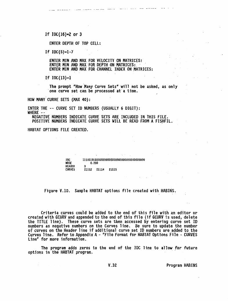
..,--..._.--_. - --- -- ..-. - ~.
If IOC(I6}-Z or 3
ENTER DEPTH OF TOP CELL:
If IOC(5)-1-7
ENTER MIN AND MAX FOR VELOCITY ON MATRICES:ENTER MIN AND MAX FOR DEPTH ON MATRICES: .ENTER MIN AND MAX FOR CHANNEL INDEX ON nATRICES:
If IOC(l3}=1
The prompt NHow Many Curve SetsNwill not be asked, as onlyone curve set can be processed at a time.
HOW MANY CURVE SETS (MAX 40):
ENTER THE -- CURVE SET ID NUMBERS (USUALLY 6 DIGIT):WHERE --
NEGATIVE NUMBERS INDICATE CURVE SETS ARE INCLUDED IN THIS FILE.POSITIVE NUMBERS INDICATE CURVE SETS WILL BE READ FROM A FISHFIL.
HABTAT OPTIONS FILE CREATED.
10C 1110010101000200000000000000000000000000NOSE 0.200HEAOER 3CURVES 21112 21114 21115
Figure V.IO. Sample HABTAT options file created with HABINS.
Criteria curves could be added to the end of this file with an editor orcreated with GCURV and appended to the end of thi s fi 1e (1 f GCURV 1s used, deletethe TITLE line). These curve sets are then accessed by entering curve set IDnumbers as negative numbers on the Curves line. Be sure to update the numberof curves on the Header line if additional curve set ID numbers are added to theCurves line. Refer to AppendiX A- NFile Format for HABTAT Options File - CURVESLineN for more information.
The program adds zeros to the end of the IOC line to allow for futureoptions in the HABTAT program.
V.32 Program MABINS

IIABINV PrograM
I. INTRODUCTION
The HABINV program builds a MBTAV options file. The following files areused along with the HABINV options file as input to HABTAV: (l) a FISHFIlcontaining criteria curves of aquatic species or recreational activities createdby the curve maintenance programs, (Z) TAPE3 containing cross sect ion data whichis output from IFG4, and (3) TP4A containing hydraulic data which is output fromIFG4. TP4A is a TP4 created·with IOC(17)*1 in the IFG4 program and then renamedTP4A by the user. This version of TP4 is in HABTAM and HABTAV readable formatrather than HABTAT readable format.
Refer to Appendix A, HABTAV Options File Format, for file format forcreating a HABINV file. Figure V.II contains a sample HABTAV input file createdby the HABINV program.
II. RUNN[NG HABINV
RHABINV,ZHABIN
ZHABIN=HABTAV options file (output)
The options are displayed and the user is asked to enter the IOC values.Typical settings for IOC values are O-OFF and I-ON. HABTAV options are describedin Table V.4 in the HABTAV program documentation.
The following prompts will appear jn the following cjrcumstances:
If [OC(6)-I or IOC(I4)-I
ENTER NOSE DEPTH:ENTER CALIBRATION PARAMETER WA":ENTER CALIBRATION PARAMETER "Bw:
If IOC(6)-Z or IOC(I4)=Z
ENTER NOSE DEPTH:
If IOC(6)=3 or IOC(14)=3
ENTER NOSE DEPTH:ENTER D65 OF BED MATERIAL:
If IOC(13)-1
The prompt "How Many Curve Sets" will not be asked as onlyone curve set can be processsed at a time.
V.33 Program MBINV

HOW MANY CURVE SETS (MAX 40):
ENTER THE -- CURVE SET 10 NUMBERS (USUALLY 6 DIGIT):WHERE --
NEGATIVE NUMBERS INDICATE CURVE SETS ARE INCLUDED IN THIS FILE.POSITIVE NUMBERS INDICATE CURVE SETS WILL BE READ FROM A FISHFIl.
If IOC{I)xl or 2
ENTER THE -- MIGRATION DISTANCES (OIST) FOR THE -- CURVESETS.
ENTER THE -- MIGRATION VELOCITIES (VLIM) TO BE SEARCHED FOR,FOR THE -- CURVE SETS.
If IOC(5H
ENTER THE .- VELOCITIES (VO) WHERE FISH HABITAT BECOMESWORTHLESS {OJ, FOR THE _. CURVE SETS.
IOC 100000000lOOOOOoooooooaoooooooooooooaoooHEADER 3ClJRYES 2l1l~ 21114 ~ll1S
DIST 20.00 10.00 15.00YLIH 1.00 2.00 3.00
Figure V.IO. Sample HABTAV options file created with HABINV.
Criteria curves could be added to the end of this file with an editor orcreated with GCURV and appended to the end of this file (If GCURV Is used, deletethe TITLE line). These curve sets are then accessed by entering curve set 10numbers as negative numbers on the Curves line. Be sure to update the numberof curves on the Header line If additional curve set 10 numbers are added to theCurves line. Refer to Appendix A- "File Format for HABTAT Options File - CURVESLine" for more information.
The program adds zeros to the end of the roc line to allow for futureoptions in the HABTAV program.
V.34 Program HABINV

HABTAE Program
I. INTRODUCTION
The HABTAE program 'calculates weighted usable area (surface or bed) orweighted usable volume (WUV) for each cross section. Weighted usable area maybe calculated one of two ways depending on the options selected; (I) weightedusable surface area (WUA) (same as HABTAT. HABTAV and HABTAM) and (2) weightedusable bed area (WUBA) which can be thought of as the weighted wetted perimetertimes a length to calculate an area. The program writes a file containing thecross section weighted usable area (surface or bed) or weighted usable volume(dependent sections), QB the weighted usable area (surface or bed) or weightedusable volume for a reach (independent cross sections) depending on the optionselected. When using the HABTAE program, WUA will refer to the weighted usablesurface area; WUBA - weighted usable bed area; and WUV ~ weighted usable volume.
For surface area and dependent cross sections. the HABTAE program willgive the same results as the HABTAT program proVided the same simulation optionsare selected.' .
Input to the HABTAE program is the options file created by the HABINEprogram and these previously created files: (I) a FISHFIl containing criteriacurves of aquatic species and/or recreational activities created by the curvemaintenance programs, (2) TAPE3 containing cross section data which is outputfrom IFG4 orWSP. and (3)TAPE4 containing hydraulic data which is output fromIFG4 or WSP. ~ that HABTAE uses a TAPE4 as input versus a TP4 as the otherhabitat simulation programs use. Also, the TAPE4 may have the cell velocitiescalculated (as per HABTAT) or have velocities calculated at the coordinate points(as per HABTAV and HABrAM).
Table V.I describes the options available in the HABTAE program. Theseoptions are selected in the HABTAE options file created. by HABINE.
V.35 Program HABTAE

Table V.I. Options In the HABTAE Program.OPTION ACTION
Oetermine. jf the weIghted u.abl. er.a {WA/. weighted usable volume {WUVl. or welghted u.able bed er..(WUBA/, is to b. calculated. and If the WA, WV. or WBA I. to be calculat.d for en Independent cro.s3ection or for a reach. If tha option to calculate WUV for an Independent cross section It selected,then the floW9 for that cross section do not have to be the same a'S for·the other eross sect tons. Ifthe WA. WUi. or WlI8A for a roech I. being oeloulated, then the flow. mu.t be the ..me from ••ctlonto $ection.
O. Calculate WUA for a teach.1 • Calculate WUA for independent GroSI sections.2 ~ Calculate WUV for ~ teach.3 '" Calculate WUV for Independent cross sect tOM.4 ~ Calculate YUBA for a teach.5 lI"Calculate VUBA for Independent croSs seeUons.
Z Print. out cro•• sect Ion deta (fr"" TAl'(3). RocOnrnend .ettlng to on. (I).
o =00 not print cross section ~ta.1 ~ Print crOS$ section data.
S Pr'lnhout the flow rel~ted data (from TAPE4) for eachcro$$ section evaluated at flach discharge. Italso lists the velocity fot each cell that has watet in it. The data ate a rehash of the WSPorIFG4output. Recommend setting to one (1).
o c Do not print flow related data.1 = Print flow related dat~.
4 Prints out all the computational details u.ed In det.rminlng the Weighted U.able Ar•• , w.lghted UsableBed Ar••• or Weighted Usable Volume. R.c.....nd settlng to zero (0) except when detail••r. needed toevaluate 'the simulation. Strongly recommend usIng only a few life stages ~nd discharges when ustngthis option, Ori the micro, the size of the output file may be a constraint.
o=Do not print computational dat~il$.1 ~ Pr1ntcomputational details.
5 Prints VUA. wtJBA, or \JOV da.ta for Individual cross: sections. Values bre autOO\atically printed tfrOe(I/-I.a, or 5; but will not be printed If IOC(I)-O.Z. or e. un1e•• IOC(5)-I.
o l:I: Do not print WUA/WUBAlWUV for e«chcross section.1 = Print WUA/WU8A1WV for each cross section.
6 Prints out the coordinates defining the critetl~ curves .. Recommend setttng to one (I}.
o ~ Do not print criteria CUtv. ooordfnates.1 ~ Pr'nt criteria curve coord1nbtes.
1 Prints out a table of the dIstribution of compo.lt••ultability feotors (C~).
If IOC(7)-I. then IOC'I} should not be .et to 1,3, or 5. lOC{n i••ut....tio.lly ••t to zero regardl•••of whet i••nt.red her. if IOC(I)-1,3, or S.
0- Do not print oompo.lte suitability factor. tabl•.t ~ Print comp~site suitability factors table.
S Defines where velocities were ~alculated on the lAPE4.
o • TAPE4 contains cell velocltle. (a. per HABrAT).1 - TAPE4 contains v.locltie••t the coordinate points
(a. per HABTAV and HA6TAH).
V.36 Program HABTAE
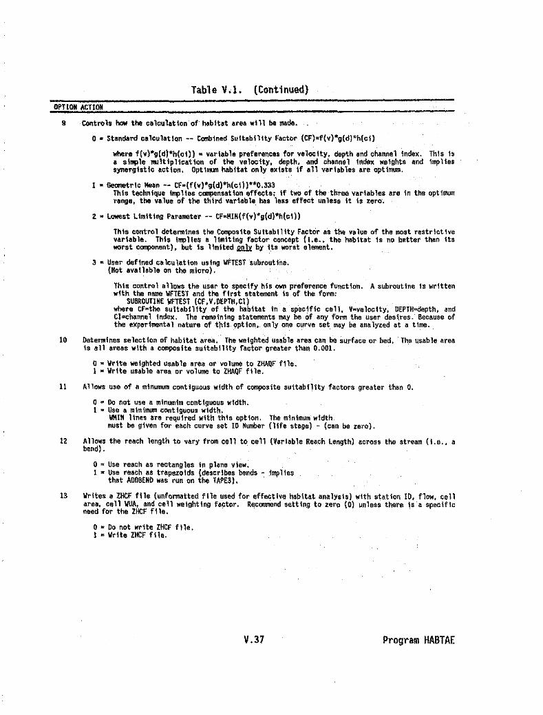
Table V.l. (Continued)OfTlOfl ACTlOfl
9 CO<Itr<>l. '- the ••l.ul.tlon of hobltat area will be made.
o - Standard calculation -- Combined Suitability Fa.tor (CF).f(v)"g(d)'h(.I)
where f(v)"g(d)'h(ol» • variable preferen.e. for v.loolty, depth and channel index. This i.a .I""le ... ltlpll.atlon of the velocity, depth. and .hannol Index weights and 1",,1I0••ynerglstlc action. Optl.... hobltat only exists if all varloble, are optimum.
1 - Geometric Kean -. CF-(f(v)'g(d)"h(cl»"O.333This technique 1..,1Ie. ccmpensatlon effects; if two of the three variables ore In the optimumrongs, the n.lue- of t~ third variable. has lest effect unless- it is zero',
Z - lowest limiting Parameter -- CF-HIH(f(v)'g(d)"h(ci)1
Thia control detenn1nes the Composite SuttabtHty Factor a's the Ybilue of the-oo,t nstrictivevariable. This Implies 0 limiting factor concept (I ••.• the habitat is no bett.r than Itsworst cOlllpOnent). but Is limited ll.Ill:t by Its wor.t element.
3 - User defined calculation using wrTEsT subroutine.(Hot ovall.ble on the micro).
This control allows the usar to specify his O\rt'rl preference function. A subroutine 1s writtenwith the nome WFTEST and the first .tatement Is of the form:
SUBROUTINE \/FTEST (CF,V.DEPTH,tllwhere cF-the suitability of the habitat In a spaciflc .call. V-velocity. DEPTfl.depth, andCf:::eMnnel index. The remaining shtetnents may be of any fom the user d&s~res. Because ofthe experimenta 1 nature Qfthi$, option•. on ly onlJ r::l,Irve set, ~y be ana lYle<! ot a time.
10 Determines selection of habitat area. The weighted usable iltea Can be surface- or bed. The usable areaia all areas with a ccmposlta .uitabllity factor greater then 0.001.
o • Write weighted Usable area or volume to ZHAQF file.1 • Vrtte usable ~rea Of volume to ZHAQF ftle.
11 Allows use of 8 minumum conttguous width of compo~ite sUitabflity faGtors greater than O.
o a Do not use a mtnum1m contiguous width.1 g Use a minimum conttguouswtdth.
WHIH line. are requlr.d With thl. option. Tho minimum widthmust be given for ea.h curva set 10 Humber (life stag.) - (cen be zero).
IZ Allows the reach length tc vary frem cell to cell (Variable Reach length) across the stream (I.e .• abend).
o = Use reach 8S rectangles tn pl~ne vtew.1 • Use reoch os trapezoids (describes bends - implies
that AlJOBEHD was run on the TAPE3). .
13 Writes a ZHCF file (unformatted file used for affective bobltat ana1ysl,) with .taticn 10, flew, cellareo, cell WUA, and cell weighting factor. RocQmmOnd setting to zero (0) un1e•• there I. a .peclflcneed for the ZHCF f l1e.
o- Do not write ZHCF file.1 • Writ. ZHCF fi1 •.
V.37 Program HABTAE

Table V.I. (Continued)OPTIOH ACTIOH
14 Control. how the velocity for the cell Is calculated. !QIl;: IOC(l4) in IWlTAE i. different thanIOC(14) in ~TAT. .
If IOC(16) Is not set to 0, then IOC114} should not be set to O.
o ct Mean column velocity.
1 - Nose velocity - Empirical ""uatlon bosed on the 1/7power law and user deftned coefftc1ents. Uter suppliesths nose depth for which a velocity Is to be calculated.and the calibration parameters Aand B. These values areentered on the HOSE line.
where: H - nos. velocity of the cellA and B ~ user defined calibration parametersV =me~n velocity of the cellON ~ noS~ depth for sPecies in qU8stiQno • total dapth of the cell
2 • Hose v.loolty - 1/7th power la. equation.User .upplie. no.e depth on HOSE line.
3 • Ho.e velocity - logarithmic velocity di.trlbutlon equation.Ths no.e depth and the 065 of the bed material are ,upplledby the u.er on the HOSE line. .
4 - Ho•• velocity - I/mth p"""r law equation.The nose veloc'ty equation used 1s
~ - (1 + ml wntmand m 1s calculated using the equation
m_!!. 0°·1667n
where VIs the mean column velocity, Vn the nos. velocity,On the no.e depth, 0 the toto I depth, n the Hanning.roughne,. coefflci.nt. and c I. 0.105 for traditions1units and 0.128 for metrio units. The value of m Isdetermln.d for .ach cell. ·The value of • and the .... depthar. given on the HOSE lIne.
5 - Ho.e velocity· l/mth power law .quatlon.S... a. IOCI14}-4 except m I, oalculated u.ln9 the equation
TIl. aDb
Values for a and bare .upplled on the HOSE line.The nose depth Is also entered on the HOSE line.
6. Hose velocity' l/mth p"""r law.quatlon.Same a. IOC(14)'4 .xcept the no.e depth (On) Is measured from the .urface.The values for nose depth and n are entered on the NOSE line.
V.38 Program HABTAE

where::
Table V.I. (Continued)OPTIOll ACTION
7 ~ Nose velocity - Shear velocity,In order to cAlculate the shear stress (,..), theMlInntng'~roughnass mu$t be known. thts value is entered on the HOSEline,
Uk ~ she~r velocityr • shear stress on the bedp • dens'ty of tke water
1S limits the velocities dl10wed tn the habitat simulation c41cul~tions. Strongly recommend setting to"0" or "I", If "Z" is selec~ed. there probably .., on orr.r in the hydroulic olmul.tlon process.
o III Abort tf velocities are __ l~ss than 0 or greater than IS.! • Convert negative veloc~tfes to positive velocities;
aborts if velocities are greater than 15.2 = No restriction on velocities.
16 Determines if given velOcities (frQlft TAP(4) Qr nose veloctth\'$ arE! usttd in habtht simlilation anddetenMtnes how those nose velocities are calculated.
If IOC(16) Is not .et to O. then IOC{14} should not be .et to 0,
If IOe(16} Is I, Z. or 3. set lOC(I7) to O.
O· Given velociti~s. or nose veloeities, (depending on whatIOC(I4) was set to} are used for nabtt~t simulation.
1 • Optimum velocities Ar~ used forhabtt~t simulationwith equal depth from top as from bottom.
A~top and bottom cellN are removed from the watercolumn. Within the remaining water column, thevelocities In the habitat simulation calculations areoptimized, t.e., it is ~ssumed that the fish can movevertically to find tho "best velocity" in tho remoinlngwater column. This Hbest velO¢lty~ 1s used with thenose velocity calculated by tho .electlon of IOC(14).If !OC(14)-O. and IOC(16)=1 .r 2. the program willcalculate noSe velocities .s if IOC(14)=2.
The "optimum (best) velocity" Is defined as thevelocity that i' found within the r.ngo .f nose "depth down from tho .urfoce (top) .nd no.e depthup from tho bottom.
Hose depth 1$ $$.t by one of two methods.a) if a NOSE line is present, nose depth
• the data supplied on the HOSE lineb) If a NOSE line is not present. n.se
depth -.1.
V.39 Program HABTAE

OPTION ACTION
Table V.1. (Continued)
Z • Optimum velocltl.s are used for habltot .Imulatlonwith unequol depth from top a. from botlom.
A"top and boltom of a ce11" or. removed from the wotercoh..... Within tha r.... lnlng .ater column. thevelocltle. In the habltot simulation ooloulatlon. areoptimized, 1.ear it is assumed that the fish oa1'! movevertioally to find the "be.t velocity' In the remainingwater coh...... Thl. 'best velocity" I. u.ed with theno.e velocity calculated by the .electlon ofIOC(14).If IOC(14)'O. and IOC(16)'1 or Z. the program willcoloulat. nos. velocltie. a. if IOC(14J'Z.
The 'bottom of the cell" Is deftned a. the nose depth. from the bottom of tho .ater column. The no.e depthIs sot on the HOSE line. If. HOSE line Is not present.nose depth •.1.
The "top of the cell" Is defined a. the distancefrom the surface of the wbter column to the depthspecified on the CELL line.
bottom' •• defined by the CELL Hne
3 • Heon velocity in a top cell is used In habitat .Imuletion.
The velocities used ate the mean velocity found in acell defined es eXisting bet..en tho surfoco of thowater column ond the dopth .peclfled on a CELL line.
17 Defines what to u&e ~$ velocity as a repleceroent far velocity. These replacements should be treated~s veloctties and be entered on the ~V~ I1neswhen entering the Curve Set Data.
If IOC(!7) I. not O. thon IOC(16) must be O.If IOC(17) 10 I or Z. then IOC(14) must be O.If IOC(!7) I. 3. then IOC(14) must be sot to 7
and Honnlng's N. 065 of bod motort.l, ond the specific grevltymust be entered on the NOSE line. If specific grevlty Is notspecified. 2.65 Is u.ed.
o w Use given velocity.! • Use velocity' depth as velocity..2 • Use (v.loclty·'Z) • depth os v.loclty3 • Use Shield's Por...ter e. velocity.
where: • Shield's psremeter- shear stress On I beda size of bed surface material at which 65% are
smaller '• specific gr.vltyof the bod material• unit weight of water
4 • Use froude NUMber as velootty.
FH • ..LJiid
whe.., V· Velocity9 *' Accelerat10n of gravityd • Depth
V.40 Program HABTAE

Table V.I. (Concluded)OPTION ACTION
18 Defines how chaonel i~dex values of zero (0) are used.
o ~ Do not use a channel index value of le~o in thecalculation of WUA for that cell.
1 =Use a channel index value of zero in the oalculationof WUA for that cell.
19 Allows the user to specify a minimum value for the composite ,suttabl1ityfactor (CF). These minimumvalues are entered on the CFMIN line.
o =No minimum comppttte suitability factor specified.1 ~ Same minimum composite suitability factor specified for all life stages.2 ~ Different minimum composite suitability factor specified fo~ each life stage.
20 Oetennines what units (traditional or metric) to w~ite the output.
o =Write output in traditional (English) units.1 = Write output In metric units.
21 Allows different loclltion of veloc1tiesor veloc1ty replacements to be IJsed for each life stage. Thisoption is basically the same dsallQwing IOC(14}. IOC(16). and IOC(l?} to be selected for each lifestage. MOTEt In this section IOC14, IOC16. and IOC17 (without parenthesis) refer to the values seton the INOSE and ONOSE .lin"". ver.us lOC(l4). IOC(l6). and IOC(l7) which refer. to the actual optionnumber.
If IOC(21) 10 not equal to zero. then IOC(l4), JOCeI6) and IOC(17) should be set to zero. If they arenot set to O. the: values entered on the nOSE and DHOS[ lines will override: the values set by IOC(l4) ,(IS). and (l1) and on the NOSE and CELL lines.
o • Use velocities that were selected by lOC(14). IOCels). and IOC(17).Same velooity for all life $tages.
I • Allow. u.lng combinations of lOC16 and IOCl7 for each life stageandspectfication as to whether mean or nose velocities (IOC14)are to be used. When using this option. lOC16 and IOC1? aremutually exclusive and are represented by the let parameteron the ONOSE line. The IOCl4 value is .et on the lNOSE line.
.ICf JOCIS IOCI7 PermissiblePARAHET£R VALUE VAlUE lOCH Values Mll2!l
0 • 0 0 O.1,2,3.4~5.6,7 Use mean or nose velocityI = I 0 1.2,3,4 Optimize velocity2 = 2 0 ),2.3.4 Optimize velocity3 = 3 0 0 Velocity· Mean velocity in top cell4 = 0 I 0 Vel. Replacement = velocity * depth5 • 0 2 0 Vel. Replacement = (velocity**2) * depthS = 0 3 7 Vel. Replacement ~ Shield's Parameter7 • 0 4 0 Vel. Replacement· Froude Number
The ONOSE 11ne contains the ICF parameter and the same infonmation as on the NOSE and CELLlines.
One INOSE line is required ,and a DNOSE ltne is required fo~ each life stage where the IOC14value on the IHOSE line is not zero.
See discussion of INOSE and DNOSE line in AppendiX A M HABTAE fonmat for more infonm4tion.
2 c Allows selecting between a nose velocity and mean columnvelocity. OneONOS£ line and one INOSE line are required.
V.41 Program HABTAE

II. RUNNING HABTAE
RHABTAE,ZHABIN,ZOUT,FISHFIL,TAPE3,TAPE4,ZHAQF,ZHCF
ZHABIN=HABINE file (input)ZOUT=HABTAE results (output)FISHFIL=unformatted curves file (input)TAPE3=unformatted cross section and reach data (input)TAPE4=unformatted flow data (input)ZHAQF=habitat vs. flow file (output)ZHCF=unformatted cell areas and cell weighted usable areasCreated if IOe(l3)=l. (output)
Figure V.12 contains sample output from the ZOUT file created by.HABTAE.Review the output file for error messages and inconsistancies in data. Errormessages in the form of notes or other statements may be written that did notappear on the screen or cause the program to abort.
Figure V.13 contains a sample ZHAQF file. The ZHCF file created whenIOC(13)=1 in HABTAE, HABTAT, or HABTAV is an unformatted file.
Ill. HABTAE ERROR MESSAGES
Refer to error messages section in HABTAT program documentation sectionas most of the error messages are the same. Most of the errors specific toHABTAE are due to illogical combinations of IOC options. When using the HABINEprogram to create the HABTAE options file, users are prompted when illogicalcombinations are entered and are instructed-to enter different option values.
V.42 Program HABTAE
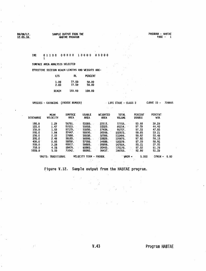
00/00/11.It.Os.58.
SAMPLE OUTPUT FROM THEHABTAE PROGllAM
loe 0 I I 0 0 0 0 0 0 0 1 0 0 0 0 0 a 0 0 01
SURFACE AREA AHALYSIS SELECTED
EFFECTIVE SECTIOH REACH LEHGTHS AHO ~EIGHTS ARE-
PROGllAM - HA6TAEPAGE - I
CIS
1.002.00
REACH
RL
77.5077 .50
155.00
PERCEHT
50.0050.00
100.00
SPECIES - KAYAKIHG (FROUDE HUMGER) LIFE STAGE - CLASS 2 CURVE 10 - 720905
MEAN SURFACE USABLE ~E1GHTEo TOTAL PERCENT PERCENTDISCHARGE VELOCITY AREA AREA AREA VOLUME USA6LE ~UA
100.0 1.29 56791. 53200. 22312. 77755. 93.66 39.29125.0 1.47 57023. 55650. 25320. 85214. 97.59 44.40150.0 1.63 57179. 55650. 2740B. 91157. 97.33 47.93200.0 1.94 57447. 56900. 30568. 102973. 99.05 53.21250.0 2.22 57698. 56900. 32566. 112494. 96.62 56.46300.0 2.48 58165. 56900. 33628. 120615. 97.82 58.15400.0 2.95 69209. 57550. 348B8. 135379. 97.20 68.92500.0 3.36 60917 . 58000. .' 35056. 147924. 95.21 57.55750.0 4.28 68478. 60000. 35443. 175170. 87.62 sL76
1000.0 5.03 71042. 66000. 36437. 196793. 92.90 51.29
UNITS: TRADITIONAL VELOCITY TERM • FROUOE WIIIH • 5.000 CFMIH • 0.00
Figure V.12. Sample output from the HABTAE program.
V.43 Program HABTAE
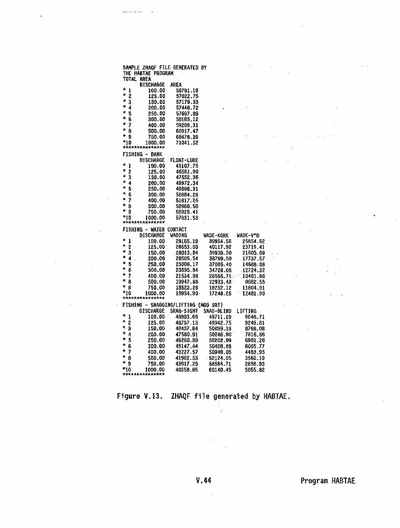
AREA56791.1957022.7557179.335744B.7257697.8958165.1259209.3160917.4766478.3971041.52
SAMPLE lHAQF FILE GENERATED BYTHE HABTAE PROGRAMTOTAL AREA
DISCHARGE, 1 100.00, 2 125.00, 3 150.00, 4 200.00, 5 250.00, 6 300.00, 7 400.00, B 500.00, 9 750.00'10 1000.00*****1l'ltlt*lIrii****FISHING - BANK
DISCHARGE, I 100.00, 2 125.00, 3 150.00, 4 200.00, 5 250.aD, 6 300.00, 7 400.00, B 500.00, 9 750.00'10 lOaD. 00***'lI*****"'*****
FLOAT-lURE45107.7546561.9047552.3648972.3449896.3150684.2651817.2552860.5055925.4157631.53
FISHING - WATER CONTACTDISCHARGE WADING
, 1 100.00 29165.19, 2 125.00 28653.00, 3 150.00 28013.04, 4 200.00 26505.54'5 250.00 25006.17, 6 300.00 23695.84, 7 400.00 21534.98, 8 500.00 19947.66, 9 750.00 18523.26'10 1000.00 15954.90**************'"
IIAIl£-KGRK39954.5640117.9239938.503B799.5037005.4034728.0628565.7122933.4319252.1217248.26
IIADE-V*O25854.6223719.4121605.8917737.5714688.0612724.3210461.869862.55
11804.9112481.90
FISHING - SNAGGING/liFTING (HOD SRT)DISCHARGE SNAG-SIGHT SNAG-BLIND
, 1 100.00 4B9B3.66 49711.19, 2 125.00 48757.13 49942.75, 3 150.00 48437.84 50099.33, 4 200.00 47580.91 50246.90, 5 250.00 46280.89 50202.99, 8 300.00 45147.44 5040B.88, 7 400.00 43227.57 50948.05, 8 500.00 41982.53 ,52124.05, 9 750.00 43017.25 58564.71'10 1000.00 40358.05 80140.45***************'
LIFTING9848.719249.818766,087816.868901.288005.774483.953560.192856.935055.82
Figure V.13. ZHAQF file generated by HABTAE.
V.44 Program HABTAE

FISHING - DRIFT BOAT (SRT)DISCHARGE PASSAGE OPERATION FlDT-PLG
, 1 100.00 44579.45 17198.51 0.00, 2 125.00 49369.38 21225.37 0.00, 3 150.00 5101l.25 24148.67 0.00, 4 200.00 54218.50 28748.37 0.00, 5 250.00 55254.78 32586.65 0.00, 6 300.00 5569a.93 35413.55 0.00, 7 400.00 5&236.12 39423.41 31.58, 8 SOO.DO 56112.09 41007.40 343.30.. 9- . 750.00 58163.49 40875.64 4620.30'10 1000.00 60932.57 38224.34 14946.34***"'*'llr~*It*.***~
WATER CONTACTOISCHARGE WADING
, 1 100,00 54370.47, 2 125.00 53265.14, 3 150.00 51951.37, 4 200.00 46992.76, 5 250.00 45856.93, 6 300.00 43158.59, 7 400.00 36627.79• 6 500.00 35642.95, 9 750.00 32934.14'10 1000.00 27577.09**Ilo***."'*****frfrRAFTING
DISCHARGE NOVICE MID-LEVEL, 1 100.00 29165.29 512.02, 2 125.00 31533.78 1298.87, 3 150.00 33277.30 1969.69, 4 200.00 40380.U 3964.57, 5 250.00 43055.14 5963.26, 6 300.00 44977.50 8469.64• 7 400.00 47640.47 12587.70• 6 500.00 47976.02 16356.92, 9 750.00 43793.64 23949.95
"10 1000.00 32306.55 26602.77.*****.***.~.**
CANOEINGDISCHARGE GENERAL NOVICE-DR MID-LEVEL
• 1 100.00 33504.90 32060.22 8398.75, 2 125.00 37215;69 34432.16 11114.16, 3 150.00 40066.06 35586.72 13766.19, 4 200.DO 44422.55 37136.16 17231.81* 5 250.00 47339.04 36401.65 19881.89* 8 300.00 49420.43 38603.48 25215.83, 7 400.00 52533.12 38119.27 29113.19* 6 500.00 54391.30 37537.97 31173.48, 9 750. DO 57174.91 34838.66 34494.l9''10 1000.00 59426.93 33303; 10 36997.50***,,"****.11;"''''***KAYM1NG (FROlOE NUMBER)
DISCHARGE CLASS 1 CLASS 2'" 1 100.00 21342.01 22312.16* 2 125.00 22022.76 25319.59* 3 150.00 22551.81 27406.12, 4 2DO.00 23447.79 30566.13'" 5- 250.00 23636.40 32586.50* 6 300.00 23909.39 33025.55* 7 400.00 23604.55 34869.26• 6 SOD. DO 23630.30 35056.50, 9 750.00 23263.56 35442.69*10 1000.00 24166.75 36436.7111<*****.**• .,•• 1\'''-
Figure V.13. (Concluded)
V.45 Program HIIBTAE

.. _ _.--.. _.. -. --_._._--- -- _._- _._-_.'
HABTAN Program
I. INTRODUCTION
The HABTAM program simulates situations in which fish can migrate 1aterallywithin a cross section in order to make use of the available weighted usable area(WUA) when there is a change in velocity.
The logic of HABTAM is similar to that of HABTAT with two major exceptions,cell definition and migration calculation. See Figure V.I for a diagram of howthe HABTAM and HABTAV programs view a cell location in contrast to how the HABTATprogram views the cell location relative to verticals. In HABTAM, cell s aredefined by one measured vertical located at the center of the cell. The valuesof stream characteristics (depth, velocity, and channel index) for each cell arethe values of the velocity, depth, and channel index at the measured vertical.
The second major difference between HABTATand HABTAM is the migrationcalculation performed by HABTAM between the user-designated starting flow anduser-designated ending flow. As in HABTAT, HABTAM calculates WUA at eachdesignated flow using functions of velocity, depth, and channel index. HABTAMassumes that the available WUA at the user-designated starting flow is fullyutilized. Considering the user-designated maximum allowable migration distancefor each life stage of each species, the progra~ ca,lcu1ates how much of theavailable WUA at the user-designated ending flow can be utilized. Fish arepermitted to migrate only laterally from cell to cell within a cross section.
The user designates a starting flow, ending flow, and a maximum allowablemigration distance for each life stage of each species. The program looks onlyat the user-designated starting and ending flows for the migration calculations,and it processes each cross section as a separate entity, that is, fish cannotmigrate from one cross section to another. Assuming that the stream is saturatedwith fish at the starting flow (all WUA, is occupied) and that the flow is thenchanged to the ending flow, the program permits the fish to migrate in eitherdirection within the cross section up to the m~ximum allowable migration distancefor the particular life stage. The program then calculates how much (the maximumamount) of the WUA available at the ending flow can be utilized by the fishpresently existing in the stream. The results will show that either all theavailable WUA at the ending flow Can be utilized, or there is an excess of WUAavailable at the ending flow which cannot be used because there are no fish touse it.
The following assumptions are made in doing the migration calculations:
1. Fish migration is assumed to begin at the cell boundaries. Thus, when afish is given a maximum allowable migration distance greater than zero,it is automatically permitted to migrate to adjacent cells. Any distanceit might have to travel within its cell of origin is negated.
2. In situations where the maximum allowab'le migration distance places a fishon the border of two cells the fish is NOT permitted access to the furthercell.
V.46 Program HABTAM

3. Since HABTAM calculates a cell width for each new flow it processes, thewidth calculated at the flow designated as the ending flow is used as thecell width for the migration calculation.
4. When a portion of a cell becomes dry at the user-designated ending flow,the fish are not permitted to migrate beyond that dry boundary point.
5. When a given life stage does not migrate at all, a value of 0.0 should beentered as the maximum allowable migration distance for that life stage.When this occurs, the program will select for the WUA with migration, theminimum of the WUA at the starting flow, and WUA at the ending flow.
Input to the HABTAM program is the options file. created by the HABINMprogram and the previously created files: (1) a FISHrIl containing criteriacurves of aquatic species or recreational activities created by the curvemaintenance programs, (2) TAPE3 containing cross section data which is outputfrom IFG4, and (3) TP4A containing hydraulic data which is output from IFG4.TP4A is a TP4 created ~ith IOC(17l"'l in the IFG.4program and then renamed TP4Aby the user. This verSlon of TP4 is in HABTAM and HABTAV readable format ratherthan HABTAT readable format.
Table V.2 describes the options available in the.HABTAM program. Theseoptions are selected in the HABTAM options file created by HABINM.
V.47 Program HABTAM

Table V.2. Options in the HABTAM.Program.OPTlOIl ACTIOIl
I Prints out details of migration caloulations. Recommend .ettlng to lero(O).
o • 00 not print migration oalculatlon details.1 • Print migration calculation detail••
2 Prints out oros. section dota (from TAPE3). Recommend setting to one (1).
D• 00 not print cross $e~tton data.1 • Print cross section dat•.
3 Prints out the flow related dota (from TP4A) for eaoh Dross section evaluated at ..chdl.cherge. Italso lists tha velocity for ..oh cell that has.ater in It. The data are a rehash of the IFG4 output.Recommend .ettlng to one (1).
o • 00 not print flow r.lated data.I • PrJnt flow related data.
4 Prints out all the computational details used In determining tha Weighted Uuble Mea. Recommendsetting to 2ero to) except when details arQ needed to evaluate the simulation. Strongly reccqne!1d USingonly a fe. life stages and discharges when using this option. On the micro. the size. of the outputfile may be a constraint.
O. 00 not print computational details.I • Print computational detail•.
5 Hot u.ed - set to '0'.
6 Scans adj.!lcent cells for:
If neither IOC(S) nor IOC(l4) equ.l. G. than they mu.t be .et to the same number.
G• Mean col"", velocity.1 • No.e velocity - Use EmpIrical equation based on
the 117th power law and user defined o..fflolenh.2 • Nose velocity - USe 1/1th pawer law equation.3 = Hose velocity - use logartthmtc velocity distribution
equation.
7 Defines how channel index values of zero (0) are used.
o ~ 00 not use a channel Index value of zero in theoalculatlon of VUA for that Dell.
I • Use a channel index value of lerO In the oalculatlonof VUA for that cell.
8 Prints out the ooordlnat•• defining the criterIa curves. Reo_d sett Ing to one (1).
o • Do not print criteria curve coordinates.1 ~ Print criteria curve coord1nates.
9 Controls how the caloulatlon of habitat area will be made.
o • Standard calculation -- combined SUitability Factor (CF).f(v)*g(d)*h(cl)
Where f(v)*g(d)*h(cI)) • variable preferences for velocity. depth and channel Index. This Isa simple ""ltlpllcatlon of the .eloclty. depth. and channel Index weights and Implle.synergistic action. Opti.... habitat only exists If all variable. are optimum.
1 • Geometric Mean -- CF.(f(v)*g(d)*h(ci))·*O.333
This technique Implies compensation effect.; if two of the three variable. are In the optimumrange. the .alue of the third variable hes less effect unless It Is lero.
V.48 Program HABTAM

Table Y.2 (Concluded)Ol'liON ACTION
2 - Lowest Limiting Parameter .- CF-HIH(f(v)'g(d)'h(oll)
This control determine. the C""""slte Sult.blllty Foetor as the .alue of the mo.t re.trioti.evariable. This Implies. limiting faotor ooncept (i.e., the habitat I. no better than It.worst c"",","ent),. but Is limited 2nll by its worst element.
a - User defined calculation using wrTEST subroutine.(Not ••ail.ble on the micro).
This control allows the user to spec1fy his own preferencefunct1Qn. A subroutine is writtenwith the nllmll wrTEST and tha first statement Is of the form:
SUBROUTINE WFTESt (CF,V.DEPTH.CI) .where CF-the suitabl11ty of the habitat In 0 specific cell. V-.eloclty. DEPTHadepth, .ndCiaohannel Index. The r....inlng stotomento may be of .ny form the user desires. Because ofthe e><perimental nature of this option, only on. curv. s.t may be .nalyzed at • time.
10 Print. the habitat .... a' a percent of totol .r... Recommend setting to on. (1).
a ~ Do not print habitat «rea ~$ a percent of total area.1 =Print habitat area es a.percent of total «rea.
11 Hot U$ed - SlJt to ....0.....
12 Allows the reach length to .ory from c.ll to cell (Variable Reech Length) acroSS the .tream (I .•.••bend).
o • Use reach as rectangles in plane view.1 - Use r.ach a' trapezoids (describes bends· impllea
that AODBEHO wa. run on the TAPE3).
13 Hot used • s.t to·O·.
14 Controls how the vsloolty for the cell Is calculated. If neither IOC(6) nor IOC(14) .quOls O. thenthey milst be set to the same numb.r.
o - Hean column •• loclty.
I - Hose v.loolty - Empiricol .quatlon based on the 1/7power law and User defined coefficients. Us.r suppliesthe nose depth for whioh ••eloclty Is to be calcul.t.d,and the calibration paramet.rs Aand B. Thes. valuas ar.entered on the HOSE lin•.
~'A [~twh.re: H - no.e velocity of the cell
Aand B • user defined calibration parameter.V - mean veloCity of the cellDN p nose depth for tpectet in questiono - tctal depth of the cell
2 .• Hese velocity· 1/7th power iaw equation.User supplle. nO.e depth on HOSE line.
a • Hose velocity - logarIthmIc velocity distribution equation.The nose depth and the 065 of the bed mat.rlal are suppll.dby the user on the HOSE line.
V.49 Program HABTAM

II. RUNNING HABTAMRHABTAM,lHABIN,ZOUT,FISHFIL,TAPE3.TP4A,lHAQF
ZHABIN-HABINM file (input)lOUT-HABTAM results (output)FISHFIL-unformatted curves file (input)TAPE3-unformatted cross section and reach data (input)TP4A=rearranged TAPE4A file (TP4 was created in HABTAM/HABTAV format
by setting IOC(17}=1 in IFG4 and was renamed TP4A by the user) (input)ZHAQF-habitat vs. flow file (output)
Figure V.14 contains sample output from the lOUT file created by HABTAM.Review the output file for error messages and inconsistancies in data. Errormessages In the form of notes or other statements maY be written that did notappear on the screen or cause the program to abort. Figure V.15 contains theZHAQF file create~ by HABTAM.
IIi. HABTAM ERROR MESSAGES
Refer to error messages section in HABTAT program documentation sectionas several of the error messages are the same. Error messages sped fi c to HABTAM.are described below.
1. INPUT LINE OF THE FORM --- WAS EXPECTED BUT --- WAS READ•.Check data set. Refer to Appendix A for "HABTAM Options File Format".
2. OPTION 6 VALUE --- AND OPTION 14 VALUE --- TO CALCULATE NOSE VELOCITY ARENOT THE SAME.If neither· IOC(6} nor IOC(I4)=0, then they must be set to the same number.
3. THE VALUE OF OPTION 14 IS .._, SINCE IT SHOULD NOT BE >3, IT HAS BEENCHANGED TO AVALUE OF 2.Values 4, 5, and 6 for iOC(14} are only available in HABTAT, not HABTAMor HABTAV.
4. ON SECTION ,-, DID NOT FIND ENOUGH VELOCITIES. DID YOU USE CORRECT OPTION(IOC(17}-I) IN IFG4?IOC(17}=1 in IFG4 writes velocities to TP4 in HABTAM and HABTAV format.TP4 must be renamed to TP4A by the user before being used as input toHABTAM or HABTAV.
5. THE STARTING FLOW -" IS NOT AVALID FLOW. THE ENDING FLOW --' IS NOT AVALID FLOW. MIGRATION CALCULATIONS FOR THE FLOW PAIR --- ARE NOT BEINGDONE.The starting and ending flows entered on the QARD lines must have beenincluded in the IFG4 data set that was used to create the TAPE3 and TP4being used as input to HABTAM.
6. CROSS SEC~ION DATA ,,- IS OUT OF SYNCH WITH Q RELATED DATA '-'.Used TAPE4 or TP4 instead of TAPE4A or TP4A; or TAPE3 or TP4A are bad: orthe TAPE3 and TP4A were not created using the same data set.
V.50 Program HABTAM

88/04/26. UPPER SALMOlI RIVER, HEAR STAMLEr, IDAHOH.05.51. IF64 DATA SET WITH IISL LINES ADDED FOIl 80TH CROSS SECTIONS FROM MANSQ
IOC 0 0 0 0 0 0 0 0 0 1 0 0 0 0 0 0 0 0 0 0
HEADER . 3 6
PRllGRAlHWlTAlIPAGE 1
CURVE 10 NUM8£RS
MAX MIGRATION OIST
21112 21114 21115
0.80 5.00 10.00
AOolTIONAL MAX MIGRATION DIST
MIGRATION FLOW PAIRS
MIGRATION FLOW PAIRS
MIGRATION FLOII PAIRS
MIGRATION FLOW PAIRS
MIGRATION FLOW PAIRS
MIGRATION FLOW PAIRS
10.00
30.00
50.00
70.00
90.00
HO.Oo
ZIl15
130.80
130.00
130.80
130.00
130.00
130.00
15.00
CURVE SET DEFINITloH DATA WAS DaTAl NED FROM THE FISHFIL FILE VHOSE TITLE LINE IS
SAMPLE flSHeRV FILE tREATED VITH THE GCURV PROGRAM
LAST UPDATED ON 88/04/25. 15.03.07.
Figure V.14. Sample output from the HABTAM program.
V.51 Program HABTAM

tlB/04/20. UPPEIl SAlHON RIYER. NEAR STANLEY, lOAHO11.05.51. IFG4 DATA SET \11TH IISl liNES AOOEO FOIl BOTH CROSS SECTIONS FRON HANSQ
Q •YS. AVAILABlE II1JA PEA 1000 FEET OF STREAIl FOR RAINBQ\I TROUT
PR06!WHfABTAMPAGE 3
Q8.00
10.0020.0030.0040.0050.0080.0070.0080.0090.00
100.00110.00 .120.00130.00
FRY1040.43893.72558.54181.5901.33
189.38263.99367.0233.6860.9895.78
259.47566.17B7B.16
JUVENILE0.000.00
81.64139.76168.90342.71426.30435.08340.37492.12587.23551.62580.97527.63
AOULT93.65
117.08193.24259.32318.73398.32504.76611.91675.69746.31613.00647.07910.33955.64
Q .YS. AYAllABlE WUA AS A PERCENTAGE OF THE GROSS AREA FOR RAIN80\1 TRour
Q8.00
10.0020.0030.0040.0050.0080.0070.0080.0090.00
100.00110.00120.00130.00
GROSS22789.24395.29444.31748.33860.39436.42618.4451Z.45820.47181.48495.49535.50843.51683.
FRY4.573.661.690.570.180.430.620.820.070.130.200.521.111.69
JUVENILE0.000.000.260.440.500.611.000.980.141.041.211.111.101.02
AOULT0.410.460.650.82Q.$41.011.161.371.471.59LBO1.711.191.64
Figure V.14. (Conti nued)
V.52 Program HABTAM

8B/04/26. UPPER SALHON RIVER. NEAR STANLEY. IOAHO11.05.51. IFG4 OATA SET WITH WSL LINES AODEO FOR BOTH CROSS SECTIONS FROM MANSQ
PROGRAM-HABTAMPA6E 4
PERMITTING FISH MIGRATION USING A BEGINNING FLOW OF 10.00UTILIZED HABITAT AREA FOR RAINBOW TROUTAT AN ENDING FLOW OF 130.00 BECOMES:
L1FESTAGE MAX ALLOIIABLE UTILIZED HABITAT AREA GROSS AREA PERCENT OF GROSS AREA PERCENT OF LIMITMIGRATION PER 1000 FEET OF STREAM USEO PER 1000 FT USED
FRY 0.00 0.00 2322. 0.00 0.00
JUVENILE 5.00 0.00 6565. 0.00 0.00
ADULT 10.00 ll6A9 165B7. 0.22 99.51
ADULT 15.00 ll6.49 16587. 0.22 99.51
PERMITTING FISH MIGRATION USING ABEGINNING fLOW Of 30.00UTILIZED HABITAT AREA fOR RAINBOW TROUTAT AN ENDING FLOW OF 130.00 BECOMES:
LIFESTAGE MAX ALLOWABLE UTILIZED HABITAT AREA GROSS AREA PERCENT OF GROSS AREA PERCENT OF LIMITMIGRATION PER 1000 FEET OF STREAM USEO PER 1000 FT USED
FRY
JUVENILE
AOULT
ADULT
0.00
5.00
10.00
15.00
0.00
138.95
260.35
260.35
2322.
6565.
16587.
16587.
0.00
0.27
0.50
0.50
0.00
99.42
100040
100.40
PERMITTING FISH MI6RATION USING A BEGINNING FLOW OF 50.00UTILIZED HABITAT AREA FOR RAINBOW TROUTAT AN ENOING FLOW OF 130.00 BECOMES:
LlFESTAGE MAX ALLOWABLE UTILIZED HABITAT AREA GROSS AREA PERCENT OF GROSS AREA PERCENT OF LIMITMIGRATION PER 1000 FEET OF STREAM USED PER 1000 fT USEO
FRY 0.00 0.00 2322. 0.00 0.00
JUVENILE 5.00 341.75 6565. 0.66 99.72
AOULT 10.00 397.69 16587. 0.77 99.89
ADULT 15.00 397.89 16587. 0.77 99.89
SECTIONS OF SAMPLE OUTPUT DELETED HERE FOR BREVITY.
Figure V.14. (Concluded)
V.53 Program HABTAM

UPPER SALMON RIVER. NEAR STANLEY. IDAHOZHAQF FILE GENERATED 8Y HARTAHTOTAL AREA
DISCHARGE AREA• 8.00 22788.89• 10.00 24395.06• 20.00 29444.04• 30.00 31741.52• 40.00 33659.Sfi• 50.00 39436.34• 60.00 42818.31• 70.00 44512.37• 80.00 45820.20• 90.00 47187.19• 100.00 48494.82• 110.00 49535.04• 120.00 50842.66* 130.00 51882.87"'''-'kjlflt••••*'''****RAINBO\I TROUT
DISCHARGE FRY JUVENILE ADULT• 8.00 1040.43 0.00 93.85• 10.00 893.72 0.00 117.06• 20.00 558.54 81.64 193.24• 30.00 181.59 139.76 259.32• 40.00 61.33 188.90 316.73* 50.00 169.38 342.71 398.32• 60.00 263.99 428.30 504.76• 70.00 367.02 435.08 611.91• 80.00 33.88 340.37 675.89• 90.00 80.98 492.12 748.31• 100.00 95.78 587.23 813.00• 110.00 259.47 551.62 847.07• 120.00 566.17 560.97 910.33• 130.00 878.16 527.63 955.84***************
Figure V.IS. ZHAQf file generated by the HABTAM program.
V.S4 Program HABTAM

HABTAT Progro
I. INTRODUCTION
The theory of the habitat simulation utilized by the HABTATprogram Isbased on the assumption that aquatic species will react to changes in thehydraulic environment. These changes are simulated for each cell ina definedstream reach. The stream reach simulation takes the form of a multi-dimensionalmatrix of the calculated surface areas of a stream having different combinationsof hydraulic parameters (i.e., depth, velocity, and channel index). Velocityand depth vary with changes in discharge causing changes in the amount ofavailable habitat. The end product of the habitat simulation is a descriptionof habitat area asa function of discharge.
There are four methods available to run the HABTAT program.
1. The recommended method is using the short form of the HABTAToptions filecreated by the HABINS program and then utilizing these previously createdfiles: (1) a FISHFll containing criteria curves of aquatic species orrecreational activities created by the curve maintenance programs, (2)TAPE3 containing cross section data resulting from an .IFG4 or WSP run, and(3) TP4 containing hydraulic data resulting from an IFG4 or WSP run.
The fo]Jowing three methods reqyire thattbe HABIN orogram be ysed to createthe long farm of the HABTAT options file with the foflowing alternatives: .
2. Utilizing a preViously created FISHF1l and entering the cross section andhydraulic data into tile options file (no TAPE3 or TP4 used as input).
3. Entering the criteria curves data into the options file and utiliZing theTAPE3 and TP4 files resulting from an IFG4 or WSP run.
4. Entering tile criteria curves data, cross section data, and hydraulic datainto the options file. No previously created files are utilized:
Table V.3 describes the options available in the HABTAT program. Theseoptions are selected in the HABTAT options file created by HABINS or HABIN.
V.55 Program HABTAT
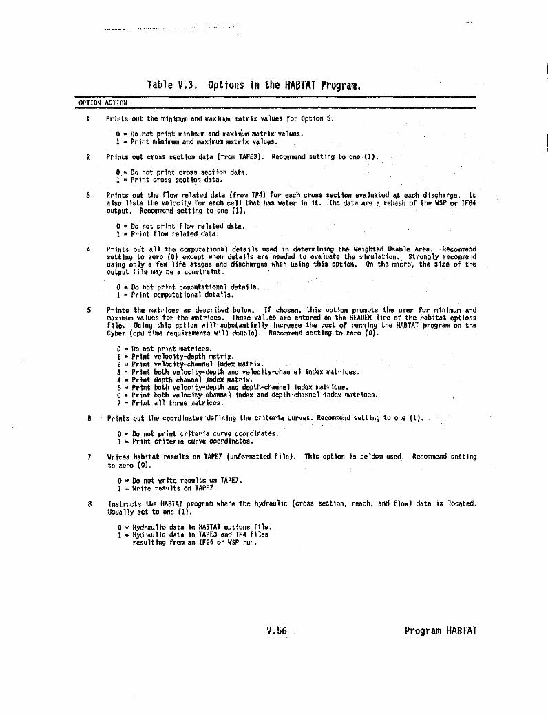
Table V.J. Options in the HABTAT Program.OPTION ACTION
I PrinU out the min\_ .nd moxlmum motr1x v.l.... for Option 5.
O. Donat prtnt minimum and maxtmummatrlx·values.1 • Print minimum and maximum matrix values.
Z prints out oro.s seotlon data (from TAPE3). Reoommend setting to on. (I).
o_~ Do not print eros, seotion data.1 = Print oross sect'on data.
3 Prints out the flow related data (from TP4) for eaoh oro.s s.otion evaluated at each disoharge. Ital.o li.ts the velooity for eaoh cell th.t ho. water in It. The data are • rehash of the WSP or IFG4output. Reoommend setting to one (I).
am Do not print flow related data.I • Print flow rel.ted data.
4 Prints out all the computational details used 1n determining: the Weighted USlible Area. RecOtTt1l8ndaettlng to zero CO) except when dBta'l1s are neede;d to eva.luate the simulation. Strongly reeomnendusing only a f~w life stages and discharges when using this option. On the micro. the size of theoutput file may be ~ Gonstra1nt.
o • Do not print computational details.I ~ Print oomputatlonal details.
5 Prints the matrices as described below. If chosen. this optlon prQrJlpts the user for minimum andrn$x1mum values for the matrices. These,v~lue$ are entered on the HEADER 11ne of the habit4t optionsfile, Using this option will substantially lnorease the oost of running the HABTAT program on theCyber (opu time requirements Will double). Recommend .ettlng to zero (0).
o =00 not _print matrices.1 • Print veloolty-depth matrix.2 ~ Print velocity-channel index matrix.3 = Print both velQClty~depth ~nd velocity-channel index matrices.4 • Print depth-channel index matrix.5. Print both veloo1ty-depth and depth-ohannel 10dsx matrloe••6 = Print both valocity-c~nn&l index and depth-channel1ndex matrices.7 = Print all three ~trices.
6 Prints out th& coordinates defining the criteri~ curves. Reoommend setting to one (1).
o ~ Do not pt1nt criteria curve ooordinates.1 = Print criteria curve coordinates.
B
Writes habitat re.ults on TAPE7 (unformotted file). Thl. option I••eldom used. Recommend settingto zero (0).
O. Do not writa tGsults on TAPEl.l' Write r••ults on TAPE].
Instructs the HABTAT rrogram where the hydraulic (cross section. reach. and flow) data is located.Usually set to one (I .
o • ~draull0 data 1n HABTAT options file.I • Hydraulio data 1n TAPE3 and TP4 fll••
resulting from an IFG4 ot WSP run.
V.56 Program HABTAT
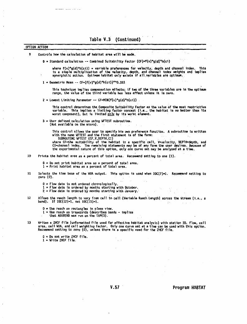
Table V.3 (Continued)OPTION ACTION
9 Controls how the ""lculatlon of habitat are. will be Ndo.
o - Standard calculation -- Combined Suitability Factor (CF)-f(v)*g(d)*h(cl)
where f(v)*g(d)*h(cl)) - vari.ble preferenc... for velnclty; depth and channa1 Index. ThisIs a sh,pl. ""ltlpllcatlon of the velocity. depth. and channel Indo. weights .nd l""lIessynergistic action. Optl.... habitat only exlsU if .11 ,variables .... optl.....
I - Geometric Hean -- CF-(f(v)*g(d)'h(cl})**0.333
This technique 1""lIe, componsatlon effectsf If two of the three variable, are In the optlo...range. the value of the third va~fable ho~ lest effeet unlet! ~t 1$ Z&to~
2 - Lowest LImIting P.rameter -- Cf-MIN(f(v)*g(d)*h(cl}}
This control dot.rmlnes the ~slt. Suitability F.ctor as the value of the """t r.strlctlvev.rlable. This Impll.' a limitIng fectorconcapt (I ••.• the habitat Is no better than Itsworst component). but Is limited 2!l1x by Its worst .l....nt.
a = U$er defined calculation using WftEST subroutine.(Not available on the micro).
This control allows the user to~pecifyhisown preferencafunctton. Asubroutfne is writtenwith the name \/FTEST and the f Ir,t .tat.....t I. of the form:
SUBROUTINE VFTEST (CF.V.DEPTH.CIIwhera Cr-the SUitability of the habitat In ••peclflc cell. V-veloolty. l!EPTH-dopth. andCIa.channel index. The rematning ,tatement$ may be of any fof'll!l the I.l$er de,1re-s. Because ofthe experimental nature of this opt ton. on.ly onec:urve set trl4y be ane.lyzed at ~ ti.lIl8.
10 Prints the habitat area as a percent of total ar". Recommend setting to on. (II.
o • Do not print habitat are~ as a pe?cent of totol !re4.1 ~ Ptint habitat are« 4' a PGrcent of total area.
II Selects the time base of the VUA output. ThIs option Is used when IOC(llal. R.c~d setting tozero (0). "
o - Flow data 1. not ordered chronologically.1 a Flow data Is ordered by months starting with October.2: '" Flow data Is ordered by lOOnths surtin; with January.
12 Allows the reach length to vary from cell to cell (Variable R.ach length) across the str""'" (1. ••••bend). If IOC(12)-I. set IOC(15}-I.
o • Use reach as rectangles in plane vtew.1 • U$8 r8AGh as t~apezo1ds (describes bends - 'mp11e~
that AOoBENO was run on the TAPE3).
13 Vrites a ZKCF file (unformatted file used for effective habItat analysis) wIth statIon 10. flow. c.llaNta. cell WUA, and cell weighting facto,.. Only one Curve sst at II time Clin be used with this option.Recommend .etting to zero (Ol. unless there I. a .peclflc need for the ZHCF file.
o - 00 not write ZKCF fIle.I a Vrlte ZHCF file.
V.57 Program HABTAT

Table V.3 (ContInued)OPTION ACTION
14 Control. how tho v.loclty for tho 0.11 i. calculat.d. If IOC(14)·4, 5. or 6, s.t IOC(16).O.
o • Mean column velocity.
1 : Hose y~locitt - Empirical equation based on the 1/7power law and user def1nedcoaff'ctent$. User suppliesthe nose depth for which aveloctty is to be calculated.and the calibration par&m&ters A &nd 6. These values areentered on the NOSE line.
where: N * nose voloc1ty of the cellA and B-user defined calibration parametersV • mean v.loclty of tho c.llOK • nose depth for s~cles 1n questiQno • total d.pth of tho c.ll
2 • No•• velocIty ~ 1/7th po.er la. equation. US'r supplle. nose depth on NOSE lin•.
3 ~ Hose velocity - logarithmic velocity distributiDn equatton.,The n08e depth ~nd the 065 of the bed material are suppliedby the user on the HOSE l\~~.
4 • Nose velooity - Shear velocity.In order to calculate the sheaf stress (~). the Manning'sroughness must be known. This value is entered on the NOSE line.
u•• .ff/p
where: U* .. shear v&locityT • shear stress on the bedp ~ density of the water
5 a Hose velocity - Shield's parameter.When using this opt1on~ Manning's roughnes~~065 9f the bed material. and the specifIc gravitymust be .ntered In the NOSE 11ne.lf specificgravity is not specified, 2.65 \s used.
r
where: .. Shield"s parameter.. shear stress on a bed~ size of bed· surface material atwhi~h 65% are
.... ll.r• specific gravity of the bed materiall<: unit weight of water
6 = No•• velocity ~ Froude number. U.ed In recreationalanalysis to gtve an \ndex to turbul~nce.
FN .. ..:LJ9d
where: Y=Velocity9 • Acceleration of gravityd =llepth
V.S8 Program HABTAT

Table V.3 (Continued)OPTIOH ACTIOH
15 Increases the calculations by abo~t 40% by not combining the total teach length assigned to a'sectione.rly in the o.laulatlon. When !OC(12).I••et IOC(IS)-I.
o ~ Combine reach lengths prior to calculations.1 ~ Do not combine reach lengths prior to calculations.
16 Oetermlnes if given velocities (from TP4 or direct entry) or nose' velQCities are used in habitatsimulation and detenmtnes how those nOS9 velocities are calculat~d. Set lOC(16).O. if lOC{14)~4. 5.or 6.
o • Given velocities, or nose veloctt1es, (depending onwhat IOC(14) waS set to) are used for habitat simulation.
1 = Optimum velocities are used for habitat simulationwith equal depth f1'OO1l top as f1'OO1l bottom.
A Wtop and bottom cell~ are removed from the watercolumn. Within the rematning water oolumn, theveloc\ties in the habitat simulation calculatiDns areoptimized. i.e .• it is assumed that the fish oan movevertically to find the Kbest velocit~ in the remainingwater column. This Nbest velocity~ is used with thenose velocity calculated by the selection of tOC(14).If 10C(14)-0. and 10C(16)-1 or 2. the program willcalculate nose velocities as if IOC(14)=2.
The "optlmUlll (bs.t) velQClty' h defined as thevelocity that is found within the r~nge of nosedepth down from the surface (top) and nose depthup from the bottQffi.
No.e depth Is set by one of two method. (a) If aNOSE line is present. nose depth = the data suppliedon the HOSE line, (bl If a HOSE line I. not pre.ent.no.e depth •. 1.
2 ~ Optimum velocities are used for habitat simulationwith unequal depth from top as from bottom.
A "top and bottom of a cell" are removed from the watercolumn. Within the remaining water cDlumn. thevelocities in the habitat $imulatiQn calculations ateoptimlled. i.e., It is a.sumed that the fish can movevertically to find the ~be$t velocity~ in the remainingwater column. This Nbest velocityN is used with thenos. v.loolty oalculated by the seleotlon of IOC(14).If IOC(14).0. and lOC(161-1 or 2. the program will~aloulate nose velocities as if IOC(14):~.
The 'bottom of the cell" 1. defined •• the nO'e depthfrom the bottom Df the water column. The nose depthi$ ~et on the HOSE line. If a NOSE line is not present.no.e depth •. 1.
The "top of the cell' 1. defined a. the distanaefrom the sutface of the water col_ to the depth.peclfled on the CEll lIne.
bottom - a. defined by the CEll line
3 ~ Mean velocity in a top cell used for habitat simulation.
The velocities used are the mean velocity found in acell defined as existing between the surface of thewatet oolumn and the depth .peclfied on a CEll line.
V.59 Program HABTAT

Table V.3 (Concluded)OPTION ACTION
17 Defines what to use as velocity. IOC(11)-t or 2 I' for use with ,orne recreaticm erttetla $lHih aswading.
o• Use gl.en velocity.1 III Usa veloolty * depth as: veloctty.2' Use (vollOClty"2) • depth .s velocity
16 Defines how .hannel Inde. values of lero (0) ore used.
o• Do not use e. cNnne1 index value of zero In thecal~u14tlon of WUA for that cell.
1 ~ Us~ a channel index value of !ero in the calculationof IIIJA for that ••n.
19 Defines how cross section weighh of zero (0) are u~.
o • Change weights of zero (0) to 0.5.1 • 00 not change zero (0) weights.
V.GO Program HABTAT

II. RUNNING HABTAT
RHA8TAT,ZHA8IN,ZOUT.fISHFIl.TAPE3,TP4.ZHAQF,ZHCF
ZHA81N-HABINS or HABIN file (input)zour-HABTAT results (output)flSIlFlL-unformatted curves fi.le (input)TAPE3=unformatted cross section and reach data (input)TP4=rearranged TAPE4file (input)ZHAQF=habitat vs. flow file (output)ZHCf=unformatted cell areas and cell weighted usable areasCreated if IOC(13)=l. (output)
Figure V.16 contains sample output from the ZOUT file created by HABTAT.Review the output file for error messages and inconsistancies in data. Errormessages·in the form of notes or other statements may be written that did notappear on the screen or cause the program to abort.
Figure V.17 contains a sample ZHAQF File. The ZHCF file created whenIOC(13)"1 in HABTAT. HABTAV. or HABTAE is an unformatted file.
III. HABTAT ERROR MESSAGES
1. LINES OUT OF ORDER, FORMAT .•. liAS EXPECTEO BUT -_. liAS OBTAINED PROCESSINGCROSS SECTION .-••Check options file. Improper sequence of format or lines, or lines calledfor by a particular option were not supplied. Refer to AppendiX A for*HABTAT Options File Format*.
2. THE NUMBER OF VELOCITIES SUPPLIED ••- FOR CROSS SECTION _•• IIHILE WORKINGON Q...-. WAS NOT ADEQUATE TO SATISFY NEEDS. TEN MORE ITEMS WILL BE ADDED,MERELY DUPUCAING ITEM GIVEN. .The velocity cells probably do not match between the TAPE3 and TP4.Reproduce TAPE3 and TP4 and re-run HABTAT.
3. IOC(I3) CAN BE ONE ONLY WHEN NUMBER OF LIFE STAGES IS ONE.IIhen generating a ZHCF file (IOC{13)=I), only one curve set may be usedat a time.
4. CROSS SEtTION DATA --- IS OUT OF SYNCH WITH QRELATED DATA _.-.Used TAPE4 instead of TP4; or TAPE3 or TP4 are bad; or the TAPE3 and TP4were not created using the same data set.
5. THE WATER SURFACE ELEVATION _.- IS _.- FEET ABOVE THE LEFT (RIGHT) .ENDPOINTOFXSEC -_.•Q..-.-. HOWEVER, SINCE THERE IS LESS THAN 10.0 FEET INVOLVEDTHE RUN IS ALLOIlEO TO CONTINUE.Message is in ZOUT file. The discharge simulated is above the lastcoordinate defining the channel. The program will continue to processQ's unless the difference is over 10 feet.
V.51 Program HABTAT

_.--,_" -- ..-..._._. - .....
6. "IfABTAT aborts and the DAYfILE on the Cyber contains an arithmaticindefinite."All curves must start with an Xvalue. 0 and end with an Xvalue· 100.
7. "IfABTAT aborts and ZOUT file contains the message "LIST EXCEEDS DATA Filename TAPE3"IOC(12)-1, therefore program expects that AODBEND has been run to addinformation to the TAPE3. Set IOC(12)-0 or run ADOBENO. '
8. CURVE SET 10 NO. INDICATED TO BE ON THE FILE .-. WAS NOT FOUND IN THEDIRECTORY FOR THE FILE.Check CURVES line in the options file to see if the correct curve set IDnumber was entered; remember curve set 10 numbers are entered as positivenumbers when they are to be read from a FISHFIl and as negative numberswhen they are to be read from the options fl1e; or one curve set 10 numberis entered on the CURVES line, but a number other than one is entered onthe HEADER line; or the FISHfIl may be bad •.
9. CURVE SPECIFIED --- WAS NOT OBTAINED FROM THE FILE ---.See #8 above.
10. THE ID NO. FOR ACURVE SET FURNISHED AS INPUT --- WAS NOT ON THE LIST OFCURVES TO BE USED.See #8 above.
11. TOO MANY CURVE SETS SPECIFIED TO BE PROCESSED ---. ONLY 40 SETS MAY BEPROCESSED IN ONE RUN.Program aborts.
12. LINES APPEAR TO BE OUT OF ORDER WHILE READING THE CURVE SET LINES FOR --,10 NUMBER -- WAS OBTAINED.When using curve sets contained in the options file, the curve setinformation must be entered in the same order as the 10 numb~rs enteredon the CURVES line(s).
13. MORE THAN 100 POINTS SPECIFIED FOR THE GROUND PROFILE --- AT SECTION ---.Program is dimensioned for 100 coordinate pairs to define a cross section.
14. MORE THAN 99 VELOCITIES HAVE BEEN SPECIFIED FOR SECTION ---.The maXimum number of coordinate points in HABIAT is 100. This means thatthe maximum number of cells is 99. Therefore, the maximum number ofvelocities per cross section is 99.
15. THE VELOCITY (DEPTH, CHANNEL INDEX) --- COULDN'T BE LOCATED IN THE LISTOF BRACKETS FOR THE MATRIX.IOC(5)"1-7 and the minimum and maximum values specified on the HEADER linein the options file could not be found.
V.62 Program HABIAI

16. INTERPOLATION NOT POSSIBLE BECAUSE THE INDEP. VARIABLE ( ---) EXCEEDS (ISLESS· THAN) THE LARGEST (SlfALLEST) VAWE IN THE TABLE (_••).A value calculated is outside the range defined by the curves in theFISHFIl. This usually Indicates that the minimum and maximum X valuesdefining a curve were not 0.0 and 100.0.
17. WEIQIfT ON SECTION -- IS GREATER THAN 1.0.Weights cannot be greater than one on a TAPE3.
18. VELOCITY EXCEEDS MAX. VEL. IN SPECIES CRITERIA TABLE 9.t VELOCITY LESS llIANMIN. VEL. IN SPECIES CRITERIA TABLE.The program only interpolates between given points. This error occurswhen all possible values are not bounded by the criteria.
19. DEPTH LESS THAN ZERO.Depths below ground (less than zero) are not permitted.
20. CROSS SECTION IDS DON'T MATCH WITHIN DATA FOR THE SECTION EXPECTED --,OBTAINED --.Check TAPE3 and TP4 to make sure theY both have the same cross section 10numbers. If hydraulic data was entered into the HABTAT options file.check to make sure consistant cross section 10 numbering was used.
V.63 Program HABTAT

88/04/26. UPPER SALMON RIVER, NEAR STAHlEr, IDAHO12.54.32. IF64 DATA SET WITH IISlllH~ ADDED FOIlIlOTH CROSS SECTIONS FROH HAN SO
******~***W~*.********.*.**.*.**.***************
• PHYSICAL HA8ITAT SIMUlATION SYSTEM •• INSTREAM .LOII GROUP, USFI/S •• . VERSIOH OF APRIL, 1988 •• RUN DATE 88/04/26. TIME 12.54.32. •**********.**.*****••••*****~****.****...***.~*
H H AAAM 888666 TTTTTTT AAAM TTTTTTTH H A A 8 8 T A A TH H A A 6 6 T A A THHHHHHH AAAAMA 888866 T AAAAAAA TH H A A 8 6 T A A TH H A A 6 6 T A A TH H A A 668868 T A A T
HADTAT PROOAAH YERSION NUNBER 4.2LAST MoDIFIED ON 26 APRIL 1988.
IDC 11100 10101 00020 00000
IOC{l)-l
PROGRAf'i-HABTATPAGE I
NUMBER OF CURYES 3
YELOCITY BRACKETS SUPPLIED 0.00 0.00SIJllDIVIOED INTO RAMGES 0.00 0.00 0.00 0.00 0.00 0.00 0.00 0.00 0.00 0.00
0.00
DEPTH BRACKETS SUPPLIED 0.00 0.00SUBDIVIDED INTO RAN6ES 0.00 0.00 0.00 0.00 0.00 0.00 0.00 0.00 0.00 0.00
0.00
CHANNEL INDEX BRACKETS SUPPLIED 0.00 0.00SUBDIVIDED INTO RANGES 0.00 0.00 0.00 0.00 0.00 0.00 0.00 0.00 0.00 0.00
0.00
CURVE ID NUMBERS 21112 21114 21115
VELOCITIES IIOV£D TO NOSE DEPTH OF 0.20 USING THE PARAMETERS0.200
(065,AN,BN.OTOP)
STATO REACH LENGTH \/EIGHT PERCENT0.0 14.25 0.30 30.00
14.3 9.97 0.50 70.00
0.000 0.000 0.000
Figure V.16. Sample output from the HABTAT program.
V.64 Program HABTAT

88/04/26. UPPER SAlMON RIVER, NEAR STANLEY, IDAHO PROGRAM-HA8TAT12.54.32. IFG4 DATA SET WITH WSL LINES ADDEO FOR 80TH CROSS SECTIONS FROM MANSQ PAGE 2
IOC(2)-1
CROSS SECTION COORD. FOR 0.00 Np. 30 NL- 14 NL- 14.25 w- 0.30
0.00 101.30 3.00 2.50 100.70 3.00 4.00 99.80 3.00 4.30 98.60 3.005.50 97.70 9.25 7.60 97.30 8.00 11.90 97.50 6.00 14.20 97.90 8.25
15.20 97.60 8.25 16.50 97.70 8.25 18.20 97.50 8.25 20.20 97.40 9.0022.20 97.30 9.00 24.20 97.20 9.00 26.20 97.30 9.00 28.20 97.50 9.0030.20 97.40 9.00 32.20 97.70 9.00 33.00 97.60 9.00 34.20 97.80 9.2535.20 97.70 9.25 36.20 97.70 9.25 37.40 97.70 9.25 39.10 97.90 10.0043.80 98.10 10.00 53.00 98.80 10.00 82.40 99.00 10.00 69.90 98.50 8.2578.10 99.00 3.00 87.10 99.50 3.00
CROSS SECTION COORD. FOR 14.30 NP, 32 NL- 20 RL. 9.97 W. 0.50
0.00 101.90 3.00 3.00 101.30 3.00 4.70 101.00 3.00 5.30 100.00 3.0015.00 100.00 3·00 19.10 99.60 3.00 29.30 99.20 3.00 33.10 98.40 3.0041.00 98.50 7.50 46.10 98.20 8.25 48.10 96.00 8.S0 48.50 97.90 8.5049.30 97.80 8.50 50.30 97.80 9.25 52.30 97.70 9.00 54.30 97.80 9.0058.30 97.80 9.00 58.30 97.60 9.00 80.30 97.60 10.00 62.30 97.60 10.0064.30 97.70 9.00 65.00 97.80 9.00 86.30 97.70 10.00 88.30 97.90 10.0070.30 98.20 10.00 73.80 98.20 10.00 77.70 98.80 10.00 86.80 99.00 10.2594.30 98.50 9.50 99.10 98.90 7.75 103.60 100.30 3.00 108.40 101.30. 3.00
88/04/26. UPPER SALMON RIVER, NEAR STANLEV, IDAHO PROGRAM-HABTAT12.54.32. IFG4 OATA SET WITH WSL LINES ADDEO FOR 80TH CROSS SECTIONS FROM HANSQ PAGE 3
Q RELATED OATA FOR THE CROSS SECTION 0.00 IDISCHARGE· 8.00 IVS • 16 \/SEL • 97.6B
VELOClTlES 0.45 0.62 0.15 0.16 0.16 0.62 1.51 1.59 1.78 2.221.90 1.40 0.63 0.42 0.54 0.12
Q RELATEO DATA FOR THE CROSS SECTION 14.30DISCHARGE • 8.00 IVS • 15 WSEL • 98.04
VELOCITIES 0.08 0.33 0.73 1.02 1.07 1.18 1.25 1.28 1.38 1.501.47 1.25 0.71 0.33 0.20
Q RELATED DATA FOR THE CROSS SECTION 0.00DISCHARGE· 10.00 IVS • 20 WSEL • 97.72
VELOCITIES 0.03 0.52 0.89 0.21 0.21 0.27 0.76 1.67 1.71 1.872.33 2.07 1.56 0.96 0.81 0.70 0.20 0.18 0.26 0.13
SECTIONS OF SAMPLE OUTPUT DELETED HERE FOR BREVITY.
Figure V.I6. (Continued)
V.65 Program HABTAT

88/04/26. ' UPPER SALMON RIVER, NEAR STANLEY, IDAHO,12.54.32. IF64 DATA SET WITH WSL LINES ADDED FOR BOTH CROSS SECTIOfIS FROII MANSO
CURVE SET DEFINITION DATA WAS 08TAINED FROII THE FISHFIL FILE WHOSE TITLE LINE IS SAIlPLE FlSHeRV FILE CREATED, WITH THE GCURV PROGRAM
LAST UPDATED ON 88/04/25. 15.03.01.
IOC(6)-1
VELOCITY WEIGHTING FOR RAINBOW TROUT
VELOCITY WEIGHTD.on 1.000.10 1.000.50 0.00
100.00 0.00
DEPTH WEIGHTING FOR RAINBOW TROUT
DEPTH WEIGHT0.00 0.000.10 0.100.20 1.000.60 1.001.00 0.601.25 0.303.on 0.00
100.00 0.00
CHANNEL INDEX WEIGHTING FOR RAINBOW TROUT
CHANNEL INDEX WEIGHT0.00 1.00
, 1.00 1.002.on 1.004.00 1.008.00 1.008.00 1.009.00 1.00
100.00 0.00
FRY
FRY
FRY
PROGRAM-HABTATPAGE 8
SECTlONS OF SAMPLE OUTPUT DELETED HERE FOR BREVlTY.
Figure V.16. (Continued)
V.66 Program HABTAT

, 88/04/26. UPPER SALMON RIVER. NEAR STAHlEY. IDAHO12.54.32. IfG4 DATA SET WITH 'OSL LINES ADDEO fOIl BOTH CROSS SECTIONS FROM NANSQ
Q VS. AVAILA8LE HABITAT AREA PER 1000 fEET Of STREAK FOR RAINBOII TROUT
Q FRY JUVENILE ADULT1 8.00 583.92 0.00 79.672 10.00 385.61 0.00 101.703 20.00 256.72 0.00 165.364 30.00 76.00 207.60 258.735 40.00 140.67 395.44 332,966 50.00 418.61 495.20 432.467 60.00 211.13 491.61 547.086 70.00 65.73 69l.28 660.669 60.00 66.67 669.96 749.36 .
10 90.00 36.96 675.61 630,3411 100.00 3.88 596.44 911.5912 110.00 0.00 512.90 970,4613 120.00 0.00 621.43 1054.9014 130.00 0.00 128.64 1113.66
66/04/26. UPPER SALMON RTVER. NEAR STANLEY. 10AHO12.54.32. IF64 DATA SET WITH WSLlINES ADOEO FOR BOTH CROSS SECTIONS FROM IlAHSQ
IOC(lO)-l
Q VS. AVAlLA6LE HABITAT AREA AS A PERCENTAGE OF THE GROSS AREA fOR RAIN60W TROUT
Q GROSS FRY JUVENILE ADUlT1 8. 22769. 2.61 0.00 0.352 10. 24395. 1.58 0.00 0.423 20. 29444. 0.67 0.00 0.634 30. 31746. 0.24 0.65 0.625 40. 33660. 0.42 1.17 0.996 50. 39436. 1.0. 1.26 1.107 60. 42616. 0.49 1.15 1.268 70. 44512. 0.15 1.55 1.469 60. 46620. 0.13 1.51 1.62
10 90. 47187. 0.08 1.43 1.7611 100. 48495. 0.01 1.23 1.6612 llO. 49535. 0.00 1.04 1.9613 120. 50843. 0.00 t.22 2.0714 130. 51883. 0.00 1.40 2.15
$$$ NORNA! COMPLETION OF JOB
Figure V.16. (Concluded)
PROGRAM-HA8TATPAGE 9
PROGRAM-HABTATPAGE 10
V.57 Program HABTAT
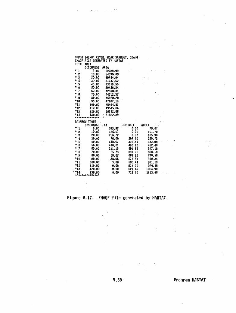
UPPER SALMON RIVER. NEAR STANLEY, IDAHOZHAQF FILE GENERATED 8Y NASTATTOTAL AREA
DISCHARGE AREA* 1 8.00 22788.9G* 2 In.08 24395.85* 3 20.80 29444.G4* 4 30.00 31747.52* 5 40.00 33659.56* 6 SO.08 39436,34* 7 60.00 42618.31* 8 70.00 44512.37* 9 80.00 45820.20*10 90.0G 47187.19*11 100.00 48494.81*12 110.00 49535.04*13 120.00 50842.68*14 130.00 51882.89'Ii'*.*:t***~.***l\"*
RAIN80W TROUTDISCHARGE
* 1 8.00* 2 10.00* 3 20.00* 4 30.00* 5 48.00* 6 50.80* 7 50.00* 8 70.00* 9 80.00*10 90.08*11 180.88*12 110.00*13 120.88
. *14 130.00*****4i*****l\f:**
FRY593.92385.51258.7276.00
140.67418.81211.1385.7358.6138.963.880.008.080.08
JUVENILE8.008.000.00
201.68395.44495.28491.81891.26889.98515.81596.44512.90621.43728.84
ADULT19.87
101.10185.98259.13332.98432.46547.08850.58740.38830.34911.59970.48
1054.901113.88
Figure V.I? ZHAQF file generated by HABTAT.
V.58 Program HABTAT

HABTAV Progrlllll
I. INTRODUCTION
The HABTAV program simulates situations where fish habitat is determinedby hydraulic parameters at the fish's location, as well as by velocities nearthe fish.
In HABTAV, cells are defined by one measured vertical located at the centerof the cell. See Figure V.I for diagram of how the HABTAY and HABTAH programsview a cell location in contrast to how the HABTAT program views the celllocation relative to verticals. The values of stream characteristics (depth,velocity, and channel index) for each cell are the values of the velocity, depth,and channel index at the measured vertical.
Option 1 in HABTAV scans the cross section a user-specified distance outfrom the cell for which the habitat is being simulated for a user-specifiedvelocity in adjacent cells. If the velocity is found Within the distance, theWUA calculated for the cell is multiplied by one. If the user-specified velocityis not found, HABTAV (With option 5 on) scans the cross section a second timefor an initial velocity. This initial velocity is the first velocity where fishhabitat is worth more than zero. HABTAV searches for a velocity between theinitial velocity and the user-specified velocity closest to the user-specifiedvelocity and then interpolates a worth for this velocity between zero and one.This worth is multiplied by WUA for a new value. If option 5 is off and theuser-specified velocity Is not found, WUA is multiplied by zero.
Input to the HABTAV program is the options file created by the HABINVprogram and these previously created files: (1) a FISHFIL containing criteriacurves of aquatic species or recreational activities created by the curvemaintenance programs, (2) TAPE3 containing cross section data which Is outputfrom IFG4, and (3) TP4A containing hydraUlic data which is output from IFG4.TP4A is a TP4 created with IOC(17)~1 in the IFG4 program and then renamed TP4Aby the user. This version of TP4 is in HABTAH and HABTAV readable format ratherthan HABTAT readable format.
Table V.4 describes the options available in the HABTAV program. Theseoptions are selected In the HABTAV options file created by HABINV.
V.69 Program HABTAV

Table V.4. Options in the HABTAV Program.
OPTIOH AmaH
1 Scan. for velocity In edjecent cell•.
a • Do not .can edjecent cell. for velocity.1 • SCans adjacent cells wtthin a user-def1ned distance
(OIST) for velocity greater then or equel to euser-defined velocity (VUH). Tf found. \I\IA forcurrent cen ... WUA * 1-
2 • Scan. adjacent cell. within a user-defined dIstance(OTST) for velocity les. than or equal to e userdefined velo<:lty (VUH). If found, \I\IA for ourrentcell - \I\IA • 1. .
Z Prints out the cross section data (from TAPEa). Recomnend setting to one (I).
o• Do not prlnt cro•• section dats.1 ~ Print cross section data.
a PrInts out the flow related deta (from TPsA) for eech eros. sectIon eveluated at each discharge.· Iteleo II,t. the velocity for each cell thet he, water In .It. The date ere a rehash of the IFG4 output.Re_d setting to one (I).
o • Do not print flow related data.I - Print flow related data.
4 Prints out ell tha computetlonal detol1. u.ed In determIning the Weighted Usable Area. Recoomendsetting to zero (0) except when details are needed to e.valuate the simulation. Strongly recomnend os'n9only a few lIfe .tages and discharge. when usIng thIs option. On the mIcro, the .Ize of the outputfll. may be a constraint.
0- Do not print computatlonsl details.I - Print computetlon,1 detell••
5 When scanning has been turned Dn byaett1ng IOC(l)-ta 1 or tt this option controls· how to calculate\I\IA In the current cell when VllH I. not found wIthin the DIST.
o- If VllM Is not found In adjacent cells, multiply WUA • O.1. if VlIM tsnot found in ~djbcent cells. scans a second
time for an Initial velocity, VO, which Is the flr.tvelocity where fl.h habitat I. greater than D. Theneearclies for, velocity between va and VlTH which I.clo..st to VlTH and Interpolata. a multIplIer for the\I\IA for the ourrent cell between 0 end 1 based on thefound velocity.
NOTES: Explanetion of the different combinations of IOC(I). lOC(5), end VD.
If IOC(lj-l, IOC(5}-I. and VO > YlIH, It i. Illogical to supply a VO. likewise.If IOC(l -Z. IOC(5}-l, and VD < VlIH, It Is illogloel to supply e VD.
~: In tho following ceses. although a va Is supplied. It is not used.
settIng IOC(I)-l. TOC(sl-l, and VD > VLIM defaults to the ssme results es .ettlng IOC(I)-lend lOC(5)-O (no Vol: end
settIng IOC(I)-2, IOC(5)-l, end VO < VllM defaults to the semu results as ••tting IOC(l)·Zand rOC(5)-D (no VD).
V.70 Program HABTAV
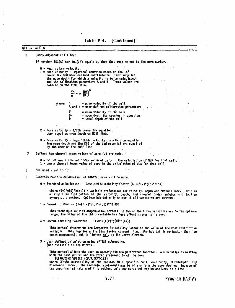
Table V.4. (Continued)OPTION ACTION
6 Scan. adjacent cells far:
If neither lOC(6) nor IOC(14) equal. 0, then they mu.t be .et to the .... number.
o• Mean column velocity.1 • No.e velocity - Emplrlcel equation ba.ed on the 1/7
pewer law and user defined coefficients. User .uppllesthe nose depth for which a velocity I. to be calculated.and the calibration parameters Aand B. These yalues areentered cn the NOSE 11 ne.
~ • A(SJI)B
where:" = nose velocity of to. cellA and B w user defined calibration parametersIi = mean veloc Ity of the cellON = nose depth for species In quest Iono = tota1 depth of the cell
2 • Nose velocity - l/lth power law equation.User supplies nOse depth on NOSE lin•.
3 ¥ HO$$ velocity - logarithmic velocity distr1button equation.The nose depth and the 065 of the bed material are suppliedby the user on the NOSE line.
7 Defines how channel index values of zero (0) ar~ used.
O· Do not use a channel Index v~lue ofzeto in the caicul$t1on of WUA for that cell.1 = U$e a channel index VAlue of zero 1n the calculation of WUA for that cell.
8 Not used - .et to "0".
9 Controls how the calculation of babltat area will be made.
o • Standard calculetlon -- Combined SUitability Faotor (CF)-f(v)*g(d)*h(ci)
where f(v)*g(d)*h(cll) • variable preferences for veloolty, depth and channel Index. This isa simple multiplication of tbe velocity, depth. and cbennel Index weights and Impll.,synergistic action. Optimum habitat only eXists If all variables are optimum.
1 - aeometrlc Mean -- CF=(f{v)*g(d)*h[cl)1**O.333
This technique implies compensation effeot,; if two Qf the three variables are in the optimumrange, the val.. of the third variable has less effect unless It Is zero.
Z = lowest limiting Parameter -- CF=HIH(f(vl*g(d)*h(cl)l
This control determInes the Composite Suitability Factor as the value of the most restrictivevariable. This lmplle. a limitIng factor concept (i.e., the habitat is no better than It.worst component). but Is limited U by Its worst element.
3 = User defined caloulatlon using WFTEST subroutine.(Hot available On the micro) •.
This control allows the user to specify his own preference function. A subroutine is writtenwith the name ~FTEST and the first statement Is of the form:
SUBROUTINE WFTEST (CF,Y,OEPTH.Cllwhere CF.the suitability of tbe bebltat In a specific cell. Y-veloclty. DEPTH-depth. andCI-channel index. The remaintng statements ~y be of any fo~ the user destres. Beoause ofthe axperiment~l nat~ra of this option, only ont eurve set may be analyzed ~t a time.
V.71 Program HABTAV
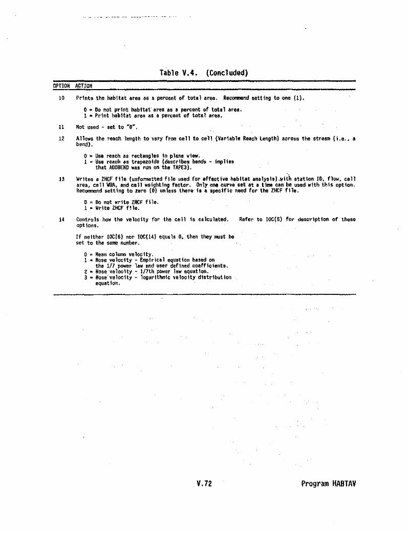
Table V.4. (Concluded)OPTION ACTION
10 Prlnto the h4bltat area a. a perc.nt of total area. Reconmend .ettlng to one (I).
a • Do not print h4bltat are. e. a perc.nt of total ar.e.1 • Print habitat area as a percent of total area.
11 Not used - set to ....0....
12 Allows the reech length to vary from cell to cell (Verlable Reach length) ecro•• the stream (I ••.• ebend) .
o u Use re~ch as rectangles in plane view.I • Us. r••ch es trepezolds (describes bends - Implle.
th4t ADDBEND wes run on the TAPE3).
13 Writes e ZHCF fil. (unformatted fil. used for .ffective habltet analy.I.).~lth station 10. flow, cellarea, cell WA. end c.ll weighting factor. Only one curve set at e time cen be used ..Ith this option.Reconmend .ettlng to zero (0) unIe•• there Is a .peclflc need for the ZHCF fll••
o • On not write ZHCF file.I • Write ZHCF file.
14 Controls how the velocity for the cell is calculated.options.
If neither IOC(6) nor IOC(14) equels O. then they must beset to the same number.
o ~ Mean column veloctty.1 a Nose velocity - Emptrical equ~tion based on
the 1/7 power 1... end u.er defined coefficients.2 • Nose velocity - 1/7th pow.r I... equatIon.S • Nos. velocity - logarIthmic velocIty distributIon
equation.
V.72
Refer to JOC(6) for description of these
Program HABTAV

II. RUNNING HABTAV
RHABTAY,ZHABIN,ZOUT,FISHFIL,TAPE3,TP4A,ZHAQF,ZHCF
ZHABIN-HABINV file (input)ZOUT..HABTAV results (output)FISHFIL-unformatted curves file (input)TAPE3-unformatted cross section and reach data (input)TP4A-rearranged TAPE4A file (TP4 was created in HABTAH/HABTAV format
by setting IOC(17)-1 in IFG4 and was renamed TP4A by the user) (input)ZHAQF~habitat vs. flow file (output)ZHCF..unformatted cell areas and cell weighted usable areaS.Created if IOC(13)-I. (output)
Figure V.18 contains sample output from the 10UTfile created byHABTAV.Review the output file for error messages and inconsistances in data. Errormessages in the form of notes or other statements may be written that did notappear on the screen or cause the program to abort.
The ZHAQF and ZHCF files are in the same format as when created by HABTAT.Figure V.19 contains the ZHAQF file created by HABTAV.
III. HABTAV ERROR MESSAGES
Refer to error messages section in HABTAT program documentation sectionas several of the error messages are the same. Error messages specific to HABTAVare described below.
1. INPUT LINE OF THE FORlt --- WAS EXPECTED BUT --- WAS READ.Check data set. Refer to Appendix A for "HABTAV Options File Format".
2. IOC(I) WAS SET TO --, JOC(l) MUST BE:o - DO NOTHING1 - SEARCH FOR VGREATER THAN OR EQUAL TO VLIM2 - SEARCH FOR V LESS THAN OR EQUAL TO VLIMValues 0, 1, and 2 are the only valid values for IOC(I} in HABTAV. Referto Table V.4 "Options in the HABTAV Program" for more information onavailable options.
3. lot(13) CAN BE ONE ONLY WHEN NUMBER OF LIFE STAGES IS ONE.When generating a ZHCF file (IOC(13}-I), only one curve set may be usedat a time.
4. CROSS SECTION DATA --- IS OUT OF SYNCH WITH QRELATED DATA _OM.Used TAPE4 or TP4 instead of TAPE4A or TP4A; or TAPE3 or TP4A is bad; orthe TAPE3 and TP4A were not created using the same data set.
V.73 Program HABTAV
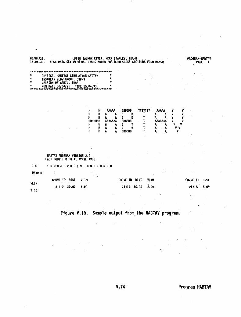
68/04/25. UPPER SAlMON RIVER. NEAR STANLEY. 10AHO15.04.33. IF64 OATA SET WITH WSL LINES AOOED FOR 60TH CROSS.SECTIOMS FROM MARSQ
*~***~***********************************~*******
• PHYSICAL HABITAT SIMULATION SYSTEM •• INSTllEAM FLOW GROUP. USfWS •• VERSION OF APRIL. 1988 •• RUN DATE 88/04/25. TINE 15.04.33. •**************.*.**~************.************.***
H H MAM 888888 TrTTrH MAM V VH H A· A 8 B T A A V VH H A A B B T A A V VHHHHHNH MMAM 88BBBB T MMAM V VH H A A B B T A A V VH H A A 8 B T A A VVH H A A 888BBB T A A V
PROGRAM-HABTAVPAGE 1
HABTAV PROGRAM VERSION 2.0LAST MODIFIED ON 11 APRIL 1968.
loe 1 0 0 0 0 0 0 0 0 1 0 0 0 0 0 0 0 0 0 0
HEADER 3
CURVE 10 OIST VUMVUN
3.0021112 20.00 1.00
CURVE 10 OIST VLIN
21114 10.00 2.00
CUllVE 10 OIST
21115 15.00
Figure V.IS. Sample output from the HABTAV program.
V.74 Program HABTAv

88/04/25. UPPER SAlHO~ RIVER. ~EAR STANlEY, IDAHO PROOllAlHIABTAV15.04.33. IFG4 DATA SET VITH VSL LI~ES ADDEO FOR BOTH ~OS5 SECTIOMS FROM MANSQ PAGE 2
CURVE SET DEFIHITIO~ DATA VAS OBTAIHEO FROM THE FISHFIL FILE WHOSE TITLE LIHE IS -
5AMPLE FlSHeRV FILE CREATED IIITH THE OCURV PROGRAM
LAST UPDATED OH 88/04/25. 15.03.07.
RA/HIlOV TROUT fRY 21112
VELOCITY DATA
VELOCIH 0.00 0.10 0.50 /00.00INDEX 1.00 LOD 0.00 0.00
DEPTH DATA
DEPTH 0.00 0.10 0.20 0.50 LOO 1.2S 3.00 100.00I~DEX 0.00 0.10 1.00 LOO 0.50 0.30 0.00 0.00
CHA~.I~OEX DATA
CHA~.INDEX 0.00 1.00 2.00 4.00 6.00 B.OO 9.00 100.00INDEX l.00 LOO 1.00 1.00 Loo l.00 1.00 0.00
88/04/Z5. UPPER SALHON RIVER. NEAR STANLEY, IDAHO PROGRAM-HABTAV15.04.33. IFG4 DATA SET IIITH IISL LINES ADDEO FOR 60TH CROSS SECTIO~S fROM NANSQ PAGE 3
RAINBOW TROUT JUVENILE 21114
VELOCITY DATA
VELOCITY 0.00 /.20 1.60 2.60 /00.00I~DEX l.00 l.00 0.25 0.00 0.00
DEPTH DATA
DEPTH 0.00 0.40 0.70 100.00INDEX 0.00 0.00 1.00 1.00
CHAN. INDEX DATA
CHAN.I~OEX 0.00 /.00 2.00 6.00 7.00 8.00 9.00 100.00I~DEX /.00 1.00 0.50 0.50 1.00 1.00 0.00 0.00
Figure V.IB. (Continued)
Y.75 Program HA6TAY

aB/04/25. UPPER SALMON RIVER, NEAR STAMLEY, IDAHO PROGRAM-HABTAY15.04.33. IFG4 DATA SET WITH WSL LINES ADDEO FOR BOTH CROSS SECTlONS FROM MANSQ PAGE 4
RAINBOW TROUT ADULT 21115
VELOCITY DATA
VELOCITY 0.00 1.50 3.00 100.00IHDEX 1.00 1.00 0.00 0.00
DEPTH DATA
DEPTH 0.00 1.00 1.60 100.00IHDEX 0.00 0.20 1.00 1.00
CHAN.IMDEX DATA
CHAN.INDE)( 0.00 1.00 2.00 6.00 7.00 8.00 9.00 100.00INDEX 0.00 1.00 0.70 0.70 1.00 1.00 0.00 0.00
Figure V.18. (Continued)
V.76 Program HABTAV

88/04/25. UPPER SALMON RIVER, NEAR STANLEY, IDAHO15.04.33. IF04 DATA SET IIITH IISL LINES AODED FOR IlDTH CROSS SECTIONS FROM MANSQ
Q .VS. AVAILA8LE HA81TAT AREA PER 1000 FEET OF STREAM FOR RAIN8011 TROUT
Q FRY JUVENILE AOULT8.00 1040.43 0.00 0.00
10.00 893.72 0.00 0.0020:00 556.54 2.03 134.6030.00 181.59 27.84 168.7240.00 61.33 80.79 316.7350.00 169.38 242.65 398.3260.00 263.99 345.68 460.1870.00 367.02 435.08 544.3780.00 33.68 340.37 588.9490.00 60.96 492.l2 041.61
100.00 95.76 587.23 685.60110.00 259.47 551.62 702.90120.00 566.17 560.97 744.92130.00 878.16 527.63 773.44
NOTE: AVAILABLE HABITAT AREA FOR FRY liAS CALCULATED BY SCANNING THEXSEC 20.00 FT. FOR VELOCITIES GREATER THAN 1.00
NOTE: AVAILA8LE HABITAT AREA FOR JUVENILE .IIAS CALCULATEO 8Y SCANNING THEX5EC 10.00 FT. FOR VELOCITIES GREATER THAN 2.00
NOTE: AVAILA8LE HA8ITAT AREA FOR ADULT liAS CALCULATES 8Y SCANNING THEXSEC 15.00 FT. FOR VELOCITIES GREATER THAN 3.00
PROGRAM-HA8TAVPA6E 5
Q .VS. AVAILABLE HA81TAT AREA AS A PERCENTAGE OF THE GROSS AREA FOR RAIN80II TROUT
Q6.00
10.0020.0030.0040.0050.0060.0070.0080.0090.00
100.00110.00120.00130.00
$$$ NORMAL COMPLETION OF HABTAV $$$
GROSS22769.24395.29444.31748.33660.39438.42818.44S12.45820.47187.48495.49535.50843.51883.
FRY4.573.661.890.570.180.430.620.820.070.130.200.521.111.69
JUVENILE0.000.000.010.090.240.620.810.980.741.041.211.111.101.02
AOULT0.000.000.460.530.941.011.071.221.291.361.411.421.47"1.49
Figure V.IS. (Concluded)
V.77 Program HABTAV

UPPER SAlHON RIVER, NEAR STAHLEY, IDAHOZHAQF FilE GENERATED BY HABTAVTOTAL AREA
DISCHARGE AREA• 8.00 2278B.89• 10.00 24395.05• 20.00 29444.04• 30.00 31747.52• 40.00 33659.56• 50.00 39436.34• 60.00 42818.31• 70.00 44512.37• 80.00 45820.20• 90.00 47187.19• 100.00 48494.82• 110.00 49535.04• 120.00 50842,66• 130.00 51892.87******t:********RAINOOll TROUT
DISCHARGE FRY JUVENilE 'ADULT• 8.00 1040.43 0.00 0.00• 10.00 893.72 0.00 0.00• 20.00 556.54 2.03 , 134.60• 30.00 181.59 27.84 158.12• 40.00 61.33 60.79 315.73 '• 50.00 169.38 242.85 398.32• 60.00 263.99 345.58 460.18• 10.00 361.02 435.08 544.31• 80.00 33.60 340.37 568.94• 90,,00 60.98 492.12 641.61• 100.00 95.78 581.23 585.60• 110.00 259.41 551.62 702.90• 120.00 565.17 560.97 144.92• 130.00 878.16 527.63 173.44..........***-***....
Figure V.19. ZHAQF file generated by the HABTAV program.
V.7a Program HABTAV

HABVD Progrllll
I. INTRODUCTION
The HABVD program is a Nshort cutNmethod of habitat simulation that usesdata readily available from the U.S. Geological Survey and the logic and conceptsof the HABTAT program. The resulting physical habitat versus streamflowrelationship is not as valuable as the standard HABTAT output, but the resultscost a lot less.
The logic of the program is basically the same as HABTAT except only onevelocity and one depth are used to represent the habitat in the stream.Specifically, the weighted usabl e area for a streamflow Q is:
WUA (Q) • A* f(v) * g(d) * h(s)
where Q. streamflowWUA • weighted usable area at the discharge Q
A· surface area per unit length (same as stream width) atstreamfl ow Q .. .
v • velocity at streamflow Qd = depth at streamflow Qs =channel index
f ( ), g ( ), h ( ) are functions dependent on the species andlife stage of interest (or recreational activity ifrecreation is of concern)
The summary of discharge measurements available for numerous gaugingstations can be used to determine the velocity, average depth, and surface width.Not a11 USGS data are useful for thi s purpose because some of the data iscollected at man-made control s such as weirs and bridges. Only data fromreasonable natural measurement points should be used with the HABVD program.
In some cases, stream morphology relationships have been developed for aspecific location - these can be used directly. Channel index information isnot available as part of the discharge measurement summaries and will have tobe obtained from some other source. One channel index value may be assignedfor the whole section of the stream being analyzed.
The stream morphology relationships are of the form:
v-kQ'"
d • c Qf
w. a Qb
V.79 Program HABVD
where v· velocity at streamflow Qd • depth at streamflow Qw- stream widthQ- streamflowk,m,c,f,a,b - coefficients (the sum of the coefficients
m,f,and b must equal wlw.)
If IOC(8)-O, the program calculates the coefficients from the datasupplied. If IOC(B)-l, the program is supplied the coefficients in the formatdescribed in Appendix A(HABVD Streamflow or Stream Morphology Parameters File).
The results from the HABVD program are different from the results fromtile HABTAT program. Examples of the different results from HABTAT and HABVDare shown in in Figure V.20. Our experience indicates the differences shownare typical.
The HABVD program was written to solve some missIng data problems and hasbeen used to determine if one set of HABTAT results could be transferreddownstream. Both cases were an appropriate use of the program. The HABVDprogram should be considered as a supplemental program to HABTAT, not as areplacement.
Table V.S describes the options available in the HABVD program. Theseoptions are selected in the HABVD options file created by HBVOIN.
v.ao Program HABVD

- Adult·
--- Juttenlfe
--- Fry
., Sl)awnlng-
as:::;0( 24Wa:I-
"' 20... II0 ~t: IS n.... E ~l- E ~... 12 f. ,0 f.til f. \\a: s Ii \\UJ Ii \I.. \I0( \\::l 4 \\3: \\
''''..00 2 4 S S 10 12 14
DISCHARGE x 1000 - of.
,/ .00 2 4 S S 10
DISCHARGE x 1000 - cl.
70 --.... _..--~ --UJ< 60 .......""\0: ........r' \~ // I ,(/)50 ,,/ I \... I f \O I I \
I I \I- 40 I f \~ I J \I;; I I \
$Of /o I I"' I Iffi ao I
.. I "0(
~
CHANNEL CATFISH· HABVD RESULTS STONECAT· HABVD RESULTS
5.
-.....--- ....:::; -- ""0( 4S / "W I "I "a: "t;; I
40 I... I
0 II
I- 32 Iu. J /1',....l- I I ......u. 24 I / ..Q I
"' I I ....Ia: 16 / ..w --.. I0( I ,....... ,....::> S ......... ,. .. "
;: ..... ' ..00 4 6 6 10 12 14
DISCHARGE x 1000 - cf. DISCHARGE x 1000 - ofs
CHANNEL CATFISH· HABTAT RESULTS STONECAT - HABTAT RESULTS
Figure V.20. HARTAT vs. HABVD program results.
V.Sl Program HABVD

Table V.5. Options in the HABVO Program.OPTION ACTION
1 Not used - set to '0'.
Z Print new velociti... depths, and discharges resulting frOM IOC(5)·0 or I.
o • Do not print new velocities, depths, and discharges.I • Print new velocities, depths, and dlscharg...
3 Print stream lI'Orpholngy relatlonshlps.
o • Do not print stream mbrphology relationships.1 • Print stream morphology relat ionships.
4 Prints out all the computational detailo 'used in determining the Weighted Usable Area. R_ndsetting ,to zero (0) except when details are needed to evaluate the o\mulat\on. Strongly rocOl1l1lOndusing only a few life steges and discharges ~hen using this option. On the micro, the size of theoutput file roay be a constraint.
o• 00 not print computational details.I =Print computational details.
5 Instructs the HABVD program where the discharge or streamflow data is located.
o • Read discharges from the Input file.1 • Detive streamflows from the ranges of discharges
on flow fl Ie.2 • Use streamflow from data puints.
6 Prints out the coordinates defining the criteria curves. Recommend setting to one (I).
o w Do not print criteria curve coordinates.1 • Print criter1~ curve coordinates.
7 Writes habitat results on TAPE7 (unfonmatted file). This option is seldom used. RecOl1l1lOnd settingto Zero (0).
o • 00 not write results on TAPE7.t • Write results on TAPE7 (.eldom used).
B Instructs the HABVO program what deta is contained In the Input file.
a = Read stream width. cross-sectional area, bod dischargefrom flow file.
t • Read stream morphology parameters from flow file.
V.82 Program HABVD

Table V.5. (Concluded)OPTION ACTInN
9 Controls how the calculation of habitat ar•• will be made.
D 0 Standard calculation -- Combined SUitability ractor (Cr)=flv)*gld)*h(cl)
where f(v)*g(d)*h(cl)l = variable preferences for velocity. depth end channel Inde~. Thl,Is a simple mUltiplication of tha velocity. depth. and channel index weights and Impliessynergistic action. Optimum habitat only e~ists If all varlabl.s are optimum.
I 0 ~tric Mean .- CFclf(v)*g(dJ*hlcl»**O.333
This technique Imp1le, compensation .ffect" If two of the three varl.bles are In the optimomr~ngBt the value of the third var1~ble has less effect unless it ts zero.
2 = low.,t limiting Paramet.r -- Cr-MIN(f(v)"g(dl*h(cil)
This control dote",,;nes the Composite Suitability Factor as the value of the most restrict Iv.varlabl.. This Implie. a limiting factor conc.pt (I .••• the h.bitat Is no better th.n itsworst componentl. but is limited 2DJx by Its WOrst element.
3 • User defined calculation using WFTEST ~ubrouttne~
(Not available On the micro).
This control allows the user tospecify.his own preference function. A subroutine is writtenwith the name WFTEST and the first statement i. of the form:
SUBROUTINE WFTEST ICr.V.DEPTH.CIIwhere Cr-the suitability of the habitat in a specific cell. V-velocity. DEPTH-depth. andCr-channel index. The remaining statements may be of any form the user desires. Because ofthe experimentol n~ture of thlsoptioo t only one curve set may be anolyzed at a time·
10· Print. the habitat are. as a percent of total area. Reconmend setting to one (I).
o B 00 not print h~b1tat-~rea aa a percent of total ~rea.
1 • Print habitat area as a Percent of total area.
V.83 Program HABVD

II. RUNNING HABVDRHABVD.lHABIN,ZIN,FISHFIL.ZOUT,ZHAQF
ZHABIN-HBVOIN file (input)liN-streamflow data or stream morphology parameters (input)FISHFIL-unformatted curves file (input)ZOUT-HABVO results (output)ZHAQF-habitat vs. flow file (output)
Refer to Appendix Afor the file format for the streamflow data or streammorphology parametersflle (lIN) which is used as input to MBVO. IfIOC(8)-O, USGS streamflow data is entered; if IOC(8)-I, stream morphologyparameters are entered.
Figure V.21 contains sample output from the ZOUT file created by MBVO.Review the output file for error messages and inconsistancies in data. Errormessages in the form of notes or other statements may be written that did notappear on the screen or cause the program to abort.
figure V.22 contains the ZHAQf file created by HABVD.
IV. HABVO ERROR MESSAGES
Most of the error messages are related to incorrect format of input files.Refer to AppendiX A (HABVD Options File Format and HABVO Streamflow and StreamMorphology Parameters File Format).
ERROR IN STREAM MORPHOLOGY SET UP OR WRONG OPTION SELECTED.If IOC(8)-O, USGS streamflow data should be contained in the ZIN input file; ifIOC(8)=I, stream morphology parameters should be contained in the ZIN inputfile.
TITLE or STREAM DATA SET IS -
SOLOMON RIVER NEAR GlEN ELDER. KANSASOATA FROM USGS OISCHARGE SUHHARY SH£ETS (\((79-81)
IOC • 0 DD0 0 0 0 0 0 I 0 0 0 0 0 0 0 0 0 000000 000 0 0 000 0 0 0 0 0 0 0
CURVES TO BE USEO ARE,
21112 21114 2111S
CURVE SET DEFINITION DATA WAS OBTAINED FROM THE FISHFIL FILE WHOSE TITLE lINE IS
SAMPLE n5HCRV FILE CllEATED WITH THE OCURV PROGRAM
LAST UPDATED DN 88/07/28. ID.47.04.
Figure V.2l. Sample output from the HABYO program.
V.B4 Program HABVO

88/08/09.08.45.58.
SOlOMOH RIVER NEAR GLEN ELDER. KANSASDATA FROIl USGS DISCHARGE SUHIIARY SHEETS (\lY79-811
DATA fOR STREAII MOIlPHOtOOY ANALYSIS
PROOllAII - ""OVOPAGE - 2
OISCHARGE31.00
122.00515.0017.4017.8013.70
VELOCITY0.901.592.001.091.280.59
DEPTlI0.782.293.950.580.381.05
WIDTH«.0033.5065.0027.51136.5022.00
RELATIONSHIP BETWEEN VELOCITY AND DISCHARGE
VELOCITY • 0.454 • DISCHARGE .. 0.245
RELATIONSHIP BETWEEN DEPTH AND DISCHARGE
DEPTH • 0.135 • DISCHARGE •• 0.548
RELATIONSHIP BETWEEN WIDTH AND DISCHARGE
WIDTH • 16.295 • DISCHARGE •• 0.207
RELATIONSHIP BETWEEN DISCHARGE AND DEPTH
DISCHARGE • 39.772 • DEPTH •• 1.4GB
Figure V.2l. (Continued)
V.85 Program HABVD
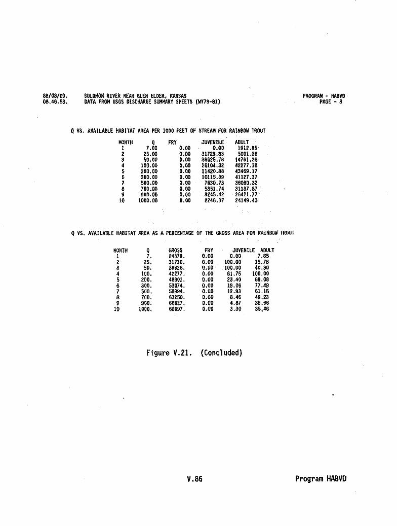
88/08/09.08.46.88.
SOLOMON RIVER NEAR 6LEN ELDER, KANSASOATA FROM USGS DISCHARGE SUMMARY SHEETS (WY79-81)
Q VS. AVAILA8LE HA8ITAT AREA PER 1000 FEET OF STREAM FOR RAIN8O\I TROUT
MONTH Q FRY JUVENILE ADULTI 7.00 0.00 0.00 1912.85'2 25.00 0.00 Sm9.83 5001.S63 50.00 0.00 36625.78 14761.264 100.00 0.00 26104.32 42277.185 200.00 0.00 11420.88 43469.176 300.00 0.00 10115.39 41127.377 500.00 0.00 7630.73 36080.328 700.00 0.00 SS51.74 31137.879 900.00 0.00 3245.42 26421.77
10 1000.00 0.00 2246.37 24149.43
Q VS. AVAILA8LE HA8ITAT AREA AS A PERCENTAGE OF THE GROSS AREA FOR RAINBDi/ TROUT
PROORAM - HA8VOPAGE - 3
HONTH Q1 7.2 25.3 50.4 100.5 200.6 300.7 SOD.a 700.9 900.
10 1000.
GROSS24379.31730.36626.42277 •48801.SS074.88994.63250.65627.68097.
FRY JUVENILE ADULTO.DD 0.00 7.85O.DD 100.00 15.76O.DD 100.00 40.30O.DD 61.75 100.000.00 23.40 89.060.00 19.06 77.490.00 12.93 61.160.00 8.46 49.230.00 4.87 S9.66O.DD 3.30 35.,46
Figure V.21. (Concluded)
V.86 Program HABVD

SOLOMOlt RIVER 8l;LOII Gt.EN ELOER DAMZHAQF FILE GENERATEO 8T THE HA8VO PROGRAMTOTAL AREA OF STREAM
OISCHARGE TOTAL AREA• 1 7.00 24318.15• 2 25.00 31128.83• 3 50.00 36625.18• 4 100.00 42271.18• 5 200.00 46600.61" 6 300.00 53013.12• 1 566.00 66993.84• 8 100.00 63248.64• 9 900.00 66521.44"10 1000.00 66096.66***.*****lIrll"••**RAINBDII TROUT
DISCHARGE FRY JUVENILE ADULT• I 7.00 0.00 0.00 1912.85" 2 25.00 0.00 31729.83 5001.38• 3 50.00 0.00 36525.18 14781.28• 4 100.00 0.00 28104.32 42271.18* 5 200.00 0.00 1I420.8l! 43489.11• 8 300.00 0.00 10115.39 41127.37• 7 566.00 0.00 7630.73 36080.32• 8 700.00 0.00 5351.74 31131.87• 9 900.00 0.00 3245.42 26421.11*10 1000.00 0.00 2248.31 24149.43....*••~ __****lIr***
Figure V.22. ZHAQF file generated by HABVD.
V.87 Program MBVO

HBWIN prograBl
I. INTRODUCTION
The HBVOIN program builds a HABVO options file. The following files areused along with the HBVOIN options file as input to HABVO: (1) a free-formattedfile containing streamflow data or stream morphology parameters and, (2) aFISHFIL containing criteria curves of aquatic species or recreational activitiescreated by the curve maintenance programs.
Refer to Appendix A (HABVO Options File Format) for file format for aHBVOIN file and for the format of the "Free-Formatted HABVO Streamflow or StreamMorphology Parameters File".
Figure V.23 contains a sample HABVO options file created by the HBVOINprogram.
II. RUNNING HBVOIN
RHBVDIN,ZHABIN
ZHABIN-HABVD options file (output)
ENTER TWO TITLE LINES (80 CHARS. MAX PER LINE):
ENTER CHANNEL INDEX (0 IF NOT USED):
One channel index value may be assigned for the whole stream.
THE FOLLOWING IOC OPTIONS ARE FOR A HABVD DATA SET
The options are displayed and the user is asked to enter the 10Cvalues.Typical settings for IOC values are O-OFF and I-ON. HABVD options aredescribed in Table V.S in the HABVD program documentation.
HOW MANY CURVE SETS (MAX 40):
ENTER THE -. CURVE SET 10 NUMBERS (USUALLY 6 DIGIT):WHERE --
NEGATIVE NUMBERS INDICATE CURVE SETS ARE INCLUDED IN THIS FILE.POSITIVE NUMBERS INDICATE CURVE SETS WILL BE READ FROM A FISHFIL.
HOW MANY FLOWS OF INTEREST?
ENTER THE -- STREAMFLOWS OF INTEREST:
HABVD OPTIONS FILE CREATED.
V.SS Program HBVOIN
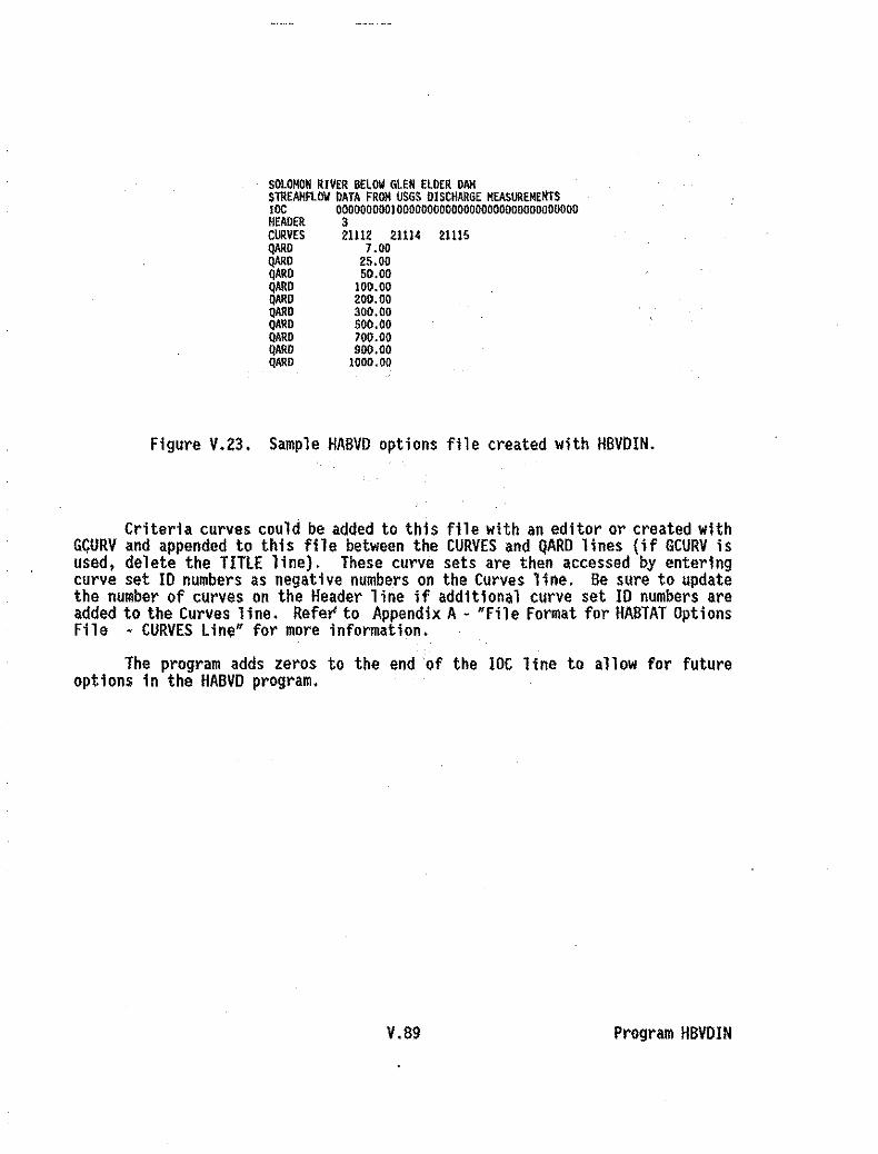
SOLOMON RIVER BELOW GLEN ElOER OAMSTREAMflOW DATA FROM USGS DISCHARGE MEASUREMENTSIDC 0000000001000000000000000000000000000000HEADER 3CURVES 21112 21114 2UI5QARO 7.00QARO 25.00QARO 50.00QARO 100.00QARO 200.00QARO 300.00QARO 500.00QARO 700.00QARO 900.00QARO 1000.00
Figure V.23. Sample HABVD options file created with HBVOIN.
Criteria curves could be added to this file with an editor or created withGCURV and appended to this file between the CURVES and QARD lines (if GCURV isused, delete the TITLE line). These curve sets are then accessed by enteringcurve set 10 numbers as negative numbers on the Curves line. Be sure to updatethe number of curves on the Header line if additional curve set 10 numbers areadded to the Curves line. Refer'to Appendix A- "File Format for HABTAT OptionsFile • CURVES line" for more information.
The program adds zeros to the end of the IOC line to allow for futureoptions in the HABVD program.
V.89 Program HBVDIN

HQF2LT Program
I. INTRODUCTION
The HQF2LT program converts a habitat versus streamflow file to a filethat is readable by LOTUS.
II. RUNNING HQF2LT
RHQF2LT,lHAQF,lOUT
lHAQF=habitat vs. flow file (input)lOUT-LOTUS readable ZHAQF file (output)
Figure V.24 contains sample output from the HQF2LT program.
'UPPER SALMON RIVER. NEAll STANLEY, IDAHO'ZHAQf FILE GENERATED BY HABTAT-TOTAL AllEA, I• 2, 3, 4, 5• 6, 1'8'9'10'Il'12'13'14
DISCHARGE8.00
10.0020.0030.0040.00SO.OO60.0070.0080.0090.00
100.00110.00120.00130.00
AllEA22188.9024395.0629444.0431147.5233659.5639436.3442818.3144512.3745620.2047181.1948494.8149535.0450842.6651882.89
Figure V.24. Sample output from the HQF2lT Program.
V.90 Program HQF2LT

LPTHqF PJ'ogl'811
I. INTRODUCTION
The lPTHQf program is a habitat simulation review program to plot thehabitat vs. flow functions - one species per page; 1-5 life stages.
The lPTHQFN program can be used to plot the habitat. vs. flow functions- one life stage per page (up to five ZHAQF files can be used as input to thelPTHQFN program). .
II. RUNNING lPTHQF
RLPTHQF.ZHAQF,ZOUT
ZHAQF*habitat vs. flow file (input)ZOUT=lPTHQF results (output)
MQ!E: On the microcomputer, graphs may be printed to the screen or to the outputfile using character graphics (132 characters per line format). In orderto use screen graphics, the computer must have a Color Graphics Adaptor(CGA) or compatible graphics card. When using screen graphics, notes arewritten to the output file in the positions where the graphs would havebeen placed had they been written using character graphics.
Figure V.25 contains sample output from the lPTHQF program.
DATE - 88/88/16. UPPER SALMON RIVER. NEAR STANLEY, IDAHOTlKE - 09.22.02. ZHAQF FILE GENERATED 8Y HABTAT
PLOTTIKG EACH LIFE STAGE OF -
RAIKBDIl TROUTA FRY8 JUVENILEC ADULT0E
Q A 8 C 0
• I 8.00 593.92 0.00 79.87• 2 10,00 385.81 0.00 101.70• 3 20.00 256,72 0.00 185.36• 4 30.00 76.00 207.60 259.73• 5 40.00 140.67 395.44 332.98* 6 50.00 418.61 495.20 432.46* 7 60.00 21L13 491.81 547.88te8 70.00 65.73 691.26 660.58" 9 80.00 58.67 689.96 740.38"10 90.00 38.96 675.61 830.34*11 100.00 3.88 596.44 91I.59*12 lID. 00 0.00 512.90 970.48"13 120.00 0.00 621.43 1054.90"14 130.00 0.00 728.64 1Il3.86
PROGRAM - LPTHQFPAGE - 3
Figure V.25. Sample output from the lPTHQF program.
V.9I Program lPTHQF
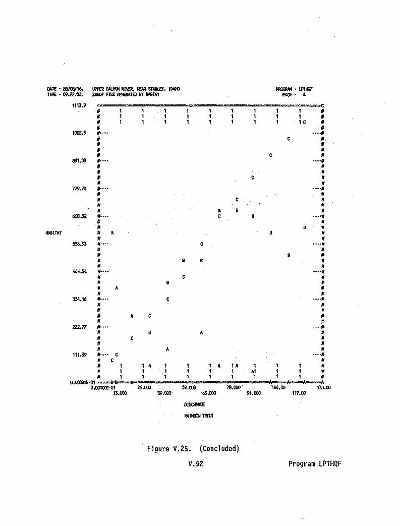
DAlE • lIlIIaV16. l.Rl£R WJOI Rl\ofR~ I£ba STANlEYk ltWI)_ .\PIIIQI'
TIlE • 09.2Z.OZ. _ FILE _TED BY III\llTAT PAG' • 4
1113.9 C/I 1 1 1 1 1 1 , II/I , 1 1 1 1 1 1 /I/I 1 1 1 , 1 1 , C /III II
'002.5 ito··· ••• 0/1/I c 1/./I II/I /I/I c II
891.09 t;. ••• ••••/1II /III II/I IIII II
m:1lJ Ifo··· ••••1/1/ 1/II C 81/ /III B B II
666.32 ito··· c B ·~~·tI
II 1/II B 1/
1II\ll1TAT II A B II1/ II
SSMJ 1/•••• c ••••1/1/ 1/II B 1/1/ B B II1/ II
445.54 /1- ••• ••• 0/1/I c /III B 1//I A /I1/ 1/
;34.16 /1-••• c ••••/11/ 1//I IIII A C IIII /I
222.77 1/•••• ••••/1/I B 1//I C 1/1/ II/I A 1/
111.39 1/•••• C ••••1/1/ C 1/1/ 1 1 A 1 1 A 1 A , , 1/1/ 1 1 1 1 , A1 1 1//I 1 1 1 1 1 1 1 1/
O.~·O1 Be 8 h , • •O.~·O1 26.00> 52.00> lll.oo> ·104.00 130.00
13.00> 39.00> 6S.1:OJ 91.00> 117.00
01_
RAll81llllWT
Figure V. 25. (Concluded)
V.92 Program lPTHQF

LPTHQFN Program
I. INTRODUCTION
The LPTHQfN program is a habitat simulation review program to plot thehabitat vs. flow functions . one life stage per page (up to five ZHAQF filescan be used as input). When more than one ZHAQF input file is specified, onecurve from each file will be plotted on the same page.
The LPTHQF program can be used to plot the habitat. vs. flow functions .one species 'per page; 1-5 life stages (only one ZHAQF file is used as input tothe lPTHQF program).
II. RUNNING lPTHQFN
RLPTHQN,ZOUT,ZHAQFl,ZHAQF2,ZHAQF3,ZHAQF4,ZHAQF5
ZOUT=lPTHQFN results (output)ZHAQF(1-5)=one to five habitat vs. flow files (input)
HQLE: On the microcomputer, graphs may be printed to the screen or to the outputfile using character graphics (132 characters per line format). In orderto use screen graphics, the computer must have a Color Graphics Adaptor(CGA) or compatible graphics card. When using screen graphics, notes arewritten to the output file in the positions where the graphs would havebeen placed had they been written using character graphics.
Figure V.26 contains sample output from the LPTHQFN program.
DATE· 88/08/16. GRAPH OF HA8ITAT VS. FLOW (ZHAQF) FILES GENERATEDTIME·09.30.32. BY HABTAT. HA8TAM, AND HABTAV
DATA SET A IS
UPPER SALMON RIVER. NEAR STANLEY. IDAHOlHAQF FILE GENERATED 8Y HA8TAT
DATA SET 8 IS
UPPER SALMON RIVER, NEAR STANLEY. IDAHOiHAQF FILE GENERATED 8Y HA8TAM
DATA SET C IS
UPPER SALMON RIVER, NEAR STANLEY, IDAHOlHAQF FIlE GENERATED 8Y HA8TAV
PROORAM . LPTHQFNPAGE -I
Figure V.26. Sample output from the lPTHQFN program.
V.93 Program lPTHQFN

IllTe' ~16. _ rA' IWlllAT '1$. FlAI C2IW'If) FII.ES tafAA1lIl_ • I.PTIIlFM
TIlE • 09.)).32. Itt IWlTAT. 1WlTIH, NO IWlTAV PAlE • 4
8Xl.00/I 1 1 1 1 1 1 /I/I 1 1 1 1 1 1 /I/I 1 1 1 1 1 1 /I/I A /I
7<0.00 /1-", ••••/1/I ,/I A A /I/I A /I/I /I
640.00 /1- ... ....,/I A /I./1 ,II C ,II II
560.00 ,I•••• C ..../1II C /III C IIII A IIII A A C /I
4/tl.lXl /1- ... •..·11II /I/I /I
IWlllAT /I B C /I/I II
400.00 /1-••• A ····11II /I/I /III C /I/I B C II
3<D.00 /1-••• ..../1II IIII /I/I II/I /I
~.OO . /1- ••• C ····11II II/I A IIII /I/I B /I
18I.lXl /1- ... ....IIII B IIII /I/I II/I II
tll.lDl /1- ... B C ..../1/I /I/I 1 1 1 1 1 1 1 1 1 /III 1 c 1 1 1 1 1 1 1 1 /I/I 1 1 1 1 1 1 1 1 1 ,
o.~·01 --.(X) CO.oo.nE·01 'G.lDl lll.lDl 120.00 160.00 200.00
;,n.lDl 60.000 100.00 1'0.00 l111.oo
PISDWllE
0JMi fal: M9lILE IlAIIIQ/ lIWT
Figure V.26. (Concluded)
V.94 Program lPTHQFN

MAKAVD Program
I. INTRODUCTION
The MAKAVD program creates an input file for the AVDEPTH program from aWSP or IFG4 data set; water surface elevations are read from a TAPE4 (generatedfrom the input data set) or entered interactively. When anIFG4 data set isconverted to an AVDEPTH data set, each cross section is divided into five'cellsof equalwfdt~.
An AVDEPTH data set is a WSP type data set with at least two additionallines added to the top. The first line contains controls for the calculationand output when the AVDEPTH program is run; the other additional lines containwater surface elevations for the cross sections. Refer to Appendix A for thefile format for an AVDEPTH data set and a sample AVDEPTH data set. This dataset was created using an IFG4 data set and the TAPE4 generated from it.
II. RUNNING MAKAVD
RHAKAVD,ZIN,ZAVIN,TAPE4
IIN~IFG4 or WSP data set (input)ZAVIN~AVDEPTH data set {output)TAPE4=unformatted flow data (optional input)
INPUT FILE FOR THE AVDEPTH PROGRAM BEING CREATEDWITH WITH THE TITLE OF-
The two title lines from the input data set will be displayed here.'
WATER SURFACE ELEVATIONS WILL BE OBTAINED FROM:(1) AJAPE4 FILE(2) DIRECT ENTRY
CHOICE:
If Option 1 is selected to read water surface elevations from a TAPE4 file:
The TAPE4 must have been generated by the data.setbeing used as input toMAKAVD.
ENTER PLOTTING CONTROL OPTION(O) NO PLOTTING(1) TO PLOT THE CROSS SECTIONS
CHOICE:
Entering #1" will generate a plot of the elevationvs. distance for eachcross section.
V.95 Program MAKAVD

ENTER NUMBER OF DEPTHS (5 MAX):
If deptlis are specified, tile AVDEPTH program will calculate the totalwidth of the stream tilat is as least as deep as tile deptll(s) specified.
ENTER THE --. DEPTHS:
Tile Velocity Calculation Control Option Is automatically set to #1# whentile water surface elevations are read from tile TAPE4 generated from tile inputdata set. Tlli s opt Ion generates data for tile #F1ow Factor" and "Vel oci ty"columns in tile AVDEPTH output for eacll cross section. Atable of tile "Summaryof Average Parameters for Whole Reach" is also generated by AVDEPTH when theVelocity Control Option is on.
If Option 2 is selected to directlY enter water surface elevations:
ENTER PLOTTING CONTROL OPTION(Ol NO PLOnING(1 TO PLOT THE CROSS SECTIONS
CHOICE:
Entering "I" will generate a plot of the elevation vs. distance for eachcross section.
ENTER VELOCITY CALCULATION CONTROL OPTION(0) DO NOT CALCULATE VELOCITIES(1) CALCULATE VELOCITIES (DISCHARGES ON THE QARD LINES MUST MATCH
WATER SURFACE ELEVATIONS ENTERED ON THE WSL LINES)CHOICE:
This option generates data for the' #Flow Factor" and "Velocity" columnsin tile AVDEPTH output for each cross section. A table of the "Summary ofAverage Parameters for Whole Reach" is also generated by AVOEPTH when theVelocity Control Option is on.
If "0" js selected:
ENTER NUMBER OF WATER SURFACE ELEVATIONS PER CROSS SECTION:
If "I" is selected:
The flows on the QARD lines are displayed and the following promptappears:
DO YOU WANT TO(1) ENTER NEW QARD LINES(2) USE EXISTING
CHOICE:
V.96 Program KAKAVO

If wlw is selected:
ENTER NUMBER OF QARD LINES:ENTER '.' FLOWS FOR THE QARD lINES:
ENTER NUMBER OF DEPTHS (S MAX):
If depths are specified. the AVDEPTH program will calculate the totalwidth of the stream that is as least as deep as the depth(s) specified.
ENTER THE _•. DEPTHS:
ENTER THE •.. ELEVATIONS FOR CROSS SECTION •.-:
V.97 Program MAKAVD

MDDIDe Program
I. INTRODUCTION
The MODIOC program changes the lOC options in the following data sets(IFG4,WSP,MANSQ) and options files (HABTAT,HABTAM,HABTAV,HABVD,HABTAE).
JUST the option numbers are modified with the MeDIOC program; not theassociated lines (i.e., NOSE Line, CELL line, etc.). For example, if MOOIoC isused to set IOC(14)=2 in HABTAT, the user will not be prompted to enter theassociated NOSE line. likewise, if IOC(14) is changed from H2" to "0", the NOSEline is not removed. Also, ALL options must be re-entered when changing optionsusing the NODIOC program. With the above considerations in mind, it may beeasier to use an editor to change the appropriate option(s) and lines.
II. RUNNING MeDIOC
RMODIOe,ZIN,ZOUT
ZIN-original data set (input)ZOUT-new data set with modified options (output)
ID DATA SET TYPE
1 HABTAT2 HABTAV3 HABTAM4 IFG45 WSP6 HABVD7 MANSQ8 HABTAE
ENTER DATA SET 10:
For example, if you wish to modify options in a WSP data set, enter "5"here. See note below for additional information on WSP options.
The options are displayed for the data set specified by the user. The user isasked to enter the IOC values.
NOTE: This is the only program where the user is prompted for the additionallines required when Options 1 or 7 are "on" in WSP (CTRI and CTRF lines).Options 2,3, and 4 also require additional lines, but the user is not promptedfor the reqUired information, as these options are not normally used in instreamflow studies. Refer to "Guide to the Application of the Water Surface ProfileComputer Program" (U.S. Bureau of Reclamation 1968) for more information on theoptions.
V.98 Program MODIOC
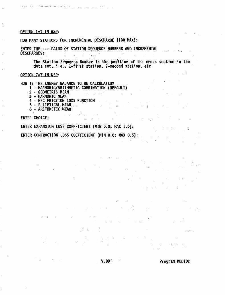
OPTION I-T IN WSP:
HOW MANY STATIONS FOR INCREMENTAL DISCHARGE (100 MAX):
ENTER THE "00 PAIRS OF STATION SEQUENCE NUMBERS AND INCREMENTALDI SCHARGES:
The Station Sequence Number is the position of the cross section in thedata set, i.e., I-first station, 2-second station, etc.
OPTION 7-T IN WSP:
HOW IS THE ENERGY BALANCE TO BE CALCULATED?I - HARMONIC/ARITHMETIC COMBINATION (DEFAULT)2 - GEOMETRIC MEAN3 0 HARMONIC HEAN·4 - HEC FRICTION lOSS FUNCTION5 0 EllIPTICAL MEAN .6 0 ARITHMETIC MEAN
ENTER CHOICE:
ENTER EXPANSION LOSS COEFFICIENT (MIN 0.0; MAX 1.0):
ENTER CONTRACTION LOSS COEFFICIENT (MIN 0.0; MAX 0.5):
V.99 Program HODIOC

SUMHQF Progru
I. INTRODUCTION
The SUMHQF program sums conditional cover columns in a ZHAQF file Into onehabitat vs. flow figure for each life stage. SUMHQF is run when conditionalcover curves were used as input to the habitat simulation programs. Up to fivelife stages can be grouped in each record (section).
II. RUNNING SUHHQF
RSUMHQF,ZHAQF,ZHAQAf
ZHAQF-habitat vs. flow file (input)ZHAQFN-modified habitat vs. flow file with columns summed (output)
Figure V.27 contains a habitat vs. flow (ZHAQF) file that was generatedby a habitat simulation program using conditional cover curves as input.
The results of running SUHHQF on this file and summing the life stages andgrouping the life stages together Is shown in Figure V.28.
The Species Line and Life stage Line for the first record in the ZHAQF fileis printed out. If the first record in the file contains UTotal Areau
information, that record is skipped as there is nothing to sum and no otherinformation should be grouped with It.
EXAMPLE:
SPECIES NAME IS: WINTER STEELHEAD - FRYLIFE STAGE NAME IS: NO COV OHC SM OBJ LG OBJ COMBO
DO YOU WANT TO SUM THESE LIFE STAGES?0) TO SUM LIFE STAGES1) TO LEAVE UNCHANGED
CHOICE:
If "0" is entered to "Sum Life Stages' -
ENTER NEW SPECIES NAME OR ,*, TO LEAVE UNCHANGED (MAX 40 CHAR):
In this case, you would probably want to change the species name to"Winter Steel head' versus "Winter Steel head - Fry".
ENTER NEW LIFE STAGE NAME OR ,*, TO USE ----- (MAX 10 CHAR):
The blank would contain the first life stage name from the record (NO COVin example above). In this example, you would probably want to change thelife stage name to "Fry".
V.IOO Program SUMHQF

The following prompt would appear !flit the first species record, BUT beforethe series of prompts for that record. Records are separated by a line of atleast 10 astericks (**********).
DO YOU WAHT THIS LIFE STAGE TO BE GROUPEDWITH THE PREVIOUS LIFE STAGE? (Y/H):
This allows grouping up to five life stages for one species into onerecord versus haVing separate records for each life stage of a species.
V.101 Program SUHHQF

ALTMAR REACH OF·SALMON RIVER. NEW YORKCOMPOSITE OF YELOCITIES AND SECTIONS AS ISLANDSTOTAL AREA
DISCMARGE AREA* 1 25.00 155830.02* 2 50.00 1774811. 70* 3 100.00 196136.69* 4 200.00 216444.92" 5 350.00 255153.21* 5 500.00 275933.49* 7 750.00 290595.31* 8 1000.00 299066.76* 9 1500.00 314227.33"10 2000.00 324867.37"II 3000.00 336215.01"12 4000.00 342061.39"13 6000.00 353205.871I***********rt"t'WINTER STEELHEAO - FRY
DISCMARGE NO COY OOC SM OBJ L60aJ CONGO" I 25.00 36804.74 15306.65 .00 21789.52 25244.11"2 50.00 42488.03 29452.52 77.77 27011.82 30049.88* 3 100.00 49470.16 52286.94 497.36 36938.97 38995.91" 4 200.00 57005.85 75435.19 1679.59 54869.38 55732.53" 5 350.00 53523.53 72839.97 11397.30 72371.30 73594.66" 6 500.00 57625.58 80575.66 13611.55 65036.53 85775.26" 7 750.00 42775.20 75005.57 17616.62 97044.67 88448.59" 8 1000.00 44224.03 56999.98 17214.27 99281.85 87951.39" 9 1500.00 33173.15 51386.56 11574.54 93601.19 84915.85"10 2000.00 30239.80 45081.72 9715.15 89553.80 78895.59"11 3000.00 41442.36 52683.58 8958.61 99457.46 85294.71"12 4000.00 40432.90 52567.05 9091.70 91380.50 74053.72"13 6000.00 38948.23 52687.85 9177.92 75138.07 53160.54*********4***'11*WINTER 5TEELHEAO • JUVENILE
D1SCHAR6E NO COV DOC 5N OBJ L6 08J" 1 25.00 8571.75 8400.63 8299.07 15146.13" 2 50.00 9510.26 9713.29 10403.51 15011.19* 3 100.00 10862.79 12095.84 12639.01 13434.02* 4 200.00 11115.55 17193.59 13461.92 9264.43* 5 350.00 8391.54 20679.94 13209.33 7143.46" 6 500.00 7582.15 22703.33 15003.20 5988.42" 7 750.00 10476.25 33439.54 17078.55 5783.53" 8 1000.00 16027.40 43305.33 18235.65 5270.12" 9 1500.00 19676.19 47712.90 16389.55 5490.25*10 2000.00 17830.52 47498.62 14551.03 4733.12"11 3000.00 367.54 27747.65 10016.22 1054.70"12 4000.00 314.97 23107.39 9085.60 481.35"13 5000.00 312.27 19565.01 7995.55 183.39***************WINTER 5TEELHEAO - ADULT
DISCHARGE NO COY OOC SN08J LG OaJ CONGO* 1 25.00 43608.82 6196.79 25572.92 68915.12 56589.43* 2 50.00 52224.68 10751.89 30262.63 73718.21 60120.13" 3 100.00 61181.60 16278.15 34279.03 72336.25 59780.00" 4 200.00 66605.23 20009.62 35725.55 64934.86 52616.65* 5 350.00 70469.46 18052.46 39403.82 64219.78 54584.10" 6 500.00 72489.76 17356.70 42968.28 64386.38 55091.62" 7 750.00 70850.33 18509.72 47208.83 60221. 78 45213.51" 8 1000.00 64313.80 15782.86 48012.24 39643.04 38723.45* 9 1500.00 56188.58 11580.82 48662.42 30564.08 34261.80"10 2000.00 53859.44 11422.69 47223.96 29356.40 33701.92"I! 3000.00 51531.37 9654.18 42808.11 34230.58 30885.99"12 4000.00 50553.69 9689.69 41964.97 33305.62 30155. I!"13 6000.00 49768.69 9994.45 43444.38 32462.49 29209.57****:t*********.
Figure V.27. ZHAQF file generated using Conditional Cover Curves.
V.I02 Program SUHliQF

AlIlWl REACH Of SALMON RIYER, NEV YORKCOMPOSITE OF VElOClTlES AND SECTIONS AS ISLANDSTOTAl AREA
DISCHARGE AREA* 1 25.00 155830.02* 2 SO.OO 1774&6.70* 3 100.00 196136.69* 4 200.00 216444.92• 5 350.00 255153.21" 6 500.00 275933.49" 7 750.00 290595.31" 8 1000.00 299066.76" 9 1500.00 314227.33
. *10 2000.00 324867.37*11 3000.00 336215.01*12 4000.00 342061.39"13 6000.00 353205.67u****__********WINTER 5TEELHEAD
DISCHARGE FRY" 1 25.00 100145.02* 2 50.00 129060.00* 3 100.00 178190.23* 4 200.00 244723.64• 5 350.00 233926.84" 6 500.00 323725.56, 7 750.00 321691.66• 8 1000.00 315571.50, 9 1500.00 274652.37'10 2000.00 253487.06"II 3000.00 287846.72*12 4000.00 267525.87*13 6000.00 229012.59"':iIt*"1I****lIt*****
JUYENIlE40417.5844836.2549032.6651035.5049424.2751277 .10
. 66777.8782338.4969269.8984723.2939196.2132990.3228057.22
AO\IlT200663.09227077.53243855.03240294.09246729.62252290.73232014.17206655.20181255.70175564.44169110.22165869.17164899.56
Figure V.28. ZHAQF file with life stages summed using SUMHQF.
V.I03 Program SUMHQF

VI. EFFECTIVE HABITAT ANALYSIS PROGRAMS
INTRODUCTION
The effective habitat analysis programs allow the user to compare theconditions in a specific cell a~ either alternative flows or for alternativespecies/life stages. The program to perform this analysis is HABEF which standsfor effective habitat given a range of streamflows.
The HABEF program has the following options:
perform an analysis combining the habitat for two life stages or species,determine the competition between two species or life stages,determine the minimum habitat available for a life stage subjectedto two flows,determine the maximum habitat available for a life stage subjected to twoflows,do an effective spawning analysis, anddo a stranding index analysis.
The HABEF program should be not confused with the effective habitatprograms that are part of the times series library of programs {TSLIB). Referto the HABEF program documentation for more information on this program.
PROGRAM BATCH/PROCEDURENAME FILENAME FUNCTION PROGRAM DESCRIPTION
HABEF RHABEF EffectiveHabitatAnalysis
VI.I
Compares two ZHCF files created whenIOC(13)=1 in HABTAT, HABTAV, orHABTAE. Comparisons available are:
1) Union of life stage2) Minimum \lUA3) Competition analysis4~ Maximum \lUA5 Minimum life stage6 Maximum life stage7) Effective spawning analysis8) Stranding index analysis
RHABEF,ZHCF1,ZHCF2,ZOUT,ZEFTBL
ZHCF1=unformatted cell areas and cellweighted usable areas (Input)
ZHCF2=unformatted cell areas and cellweighted usable areas (input)
ZOUT=HABEF results (output)ZEFTBL=file similar to a ZHAQF filewhen Options 1,3,5, or 6 areselected; two-flow habitat tablewhen Option 2,4,7, or 8 isselected. (output)

LISTINg INEQRMaTIQN ERDK AZHCF FILEPROGRAM BATCH/PROCEDURE
NAME FILENAME FUNCTJOH
LSTHCF RLSTHCF ZHCF Filelisting
PROGRAM DESCRIPTION
L1 sts the contents of a ZHCF fi1 e withvarious options. These optionsinclude: listing the title and speciesname, creating a fil e with the habitatvs. flow relationship (ZHAQF) , determining the accumulative distributionof the composite suitability of usefactors, and the listing of all cellfactors.
lSTCfl RlSTCEl ZHCF FileUsting
VI.2
RLSTHCF,lHCF,lOUT,lCEl,~QF
lHCF-unformatted cell areas and cellweighted usable areas (input)
lOUT-accumulative distribution ofcomposite suitability of use factors(outplJt) .
lefl-cell factors file (output)ZHAQF=habitat vs. flow file (output)
lists the SUitability of use factorsfor each cell in a pattern resemblinga map. Th is allows for the comparl sonof factors In adjacent cells and howthe factors for a cell vary withdischarge. A "map" for each crosssection is generated.
RlSTCEL,ZHCF,TAPE3,ZOUT
lHCF=unformatted cell areas and cellweighted usable areas (input)
TAPE3=unformatted cross section andreach data (input)
ZOUT-lSTCEl results (output)

MISCELLANEOUS lUCF FILE PROGRAMS
PROGRAM BATCH/PROCEDURENAME FILENAME FUNCTION
EXTCF
PLOTCF
TRNHCF
REXTCF
RPLOTCF
RTRHHCF
ZHCF File -Miscel1aneous
,ZHCF File -Miscellaneous
ZHCF File -Mi seellaneous
VI.3
PROGRAM DESCRIPTION
Creates an input file for the PlOTCFprogram Which plots composite suit·ability weighting factors.
REXTCF,TAPE3,TAPE4,ZHCF,ZCF
TAPE3-unformatted cross section andreach data {input}
TAPE4-unformatted flow data (input)ZHCF-unformatted fil e witll cell areas
and cell weighted usable areas(input)
ICF-composite suitability weightingfactors data (output)
Plots the composite SUitabilityweighting factors file {ZCF} createdby tile EXTCF program. This programis only available on the micro. Themi crocomputer must have the capabi1ityto display CGA {640 x 200} graphics.
RPLOTCF,ZCF
ZCF=composite SUitability weightingfactors data {input}
Converts an unformatted ZHCF file toa formatted ZHCF file; or converts aformatted ZHCF file to an unformattedZHCF file.
RTRHHCF,ZHCF,ZHCFN
ZHCF-unformatted or formatted fileof cell areas and cell weightedusable areas (input)
ZHCFN-new ZHCF file that is eitllerformatted or unformatted dependingon whether the input file wasformatted or unformatted (output)

lWUlULAIlHG Amni.Ill.EPROGRAM BATCH/PROCEDURE
NAME FILENAME FUNC]IQN
MKEHQF RMKEHQF ZEFTBL FileManipuation
MRGEFT RMRGEFT ZEFTBl FileManipUlation
PRQGBAM DESCRIPTIQN
Creates two habitat vs. flow (ZHAQF)files from the two-flow habitat table(ZEFTBl file) created by HABEFwhenOption 2,4,7, or 8 is selected.
RKKEHQF,ZEFTBl,ZHAQFl,ZHAQF2
ZEFTBl~two-flow habitat table (input)ZHAQFl~habitat vs. flow file with upto five columns per "speciesequivalent" section (output)
ZHAQF2=habitat vs. flow file with onecolumn per "species equlvalent"section (output)
Merges two two-flow habitat tables(ZEFTBl files), created by HABEF whenOption 2.4.7. or 8 Is selected.
RMRGEFT,ZEFTBLI,ZEFTBl2,ZEFTBLN,ZOUT
ZEFTBLl=two-flow habitat table(input)
ZEFTBL2=two-flow habitat table(Input)
ZEFTBlN=new ZEFTBl file (output)ZOUT=matrix table of the combined
ZEFTBl files (output)
VIA

EXTCF Program
I. INTRODUCTION
The EXTCF program creates an input file for the PLOTCF program which plotscomposite suitabil ity weighting factors. This allows one to examine thecomposite habitat suitability index for each cell of each cross section at eachsimulated flow for a single life stage.
The PlOTCF program. is only available on the microcomputer. In order to runPlOTCF, the microcomputer must have the capability to display CGA (640 x 200graphics).
Input to EXTCF is a TAPE3 containing cross section and reach data and aTAPE4 containing flow data; these two files are output from the hydraul icsimul ation process and were used as input to the habitat simul ation programsHABTAT, HABTAV, or HABTAE. The ZHCF file is created by setting IOC(13)=I inHABTAT, HABTAV, or HABTAL
II. RUNNING EXTCF
REXTCF,TAPE3,TAPE4,ZHCF,ICF
TAPE3=unformatted cross section and reach data (input)TAPE4=unformatted flow data (input)ZHCF=unformatted cell areas and cell weighted usable areas (input)ZCF=composite suitability weighting factors data (output)
VI.S Program EXTCF

HABEF Progrill1l
I. INTRODUCTION
The HABEF program calculates the physical habitat considering theconditions at two streamflows and/or for two life stages or species of fish.The program uses two ZHCF fil es created by the HABTAT, HABTAV, or HABTAEprograms, when IOC(13)-I, as input. In some cases, the second ZHCF file is acopy of the first. In other cases the files are for different life stages forthe same species or, they may be for different species.
The information in each ZHCF file consists of information for each cell.The basic equation used in HABTAT, HABtAV, and HABTAE is that the usability ofa cell, i, is given by the equation
WUA(i) - A(i) * CF(i)
where CF is some function of the velocity, depth, and the channel index for thecell. The information written to the ZHCF file> consists of A(i) and CF(i) foreach cell used in the physical habitat simulation.
The Weighted Usable Area (WUA) term as used in HABEF Is defined by theequation
ncellWUA " }; CF j Aj
i-I
where CF is the suitability factor based on velocity, depth, and a channel index,and A is the area of a wet cell. The usable area (UA) is
ncellUA " };
i-I
IF(CF ~ 0.001) UA j - Ai
IF(CF < 0.001) UA j " 0.0
Options in the HABEF program are:
1. UNION OF LIFE STAGE 1 WITH LIFE STAGE 22. STREAMFLOW VARIATION ANALYSIS (MINIMUM WUA)3. COMPETITION ANALYSIS4. STREAMFLOW VARIATION ANALYSIS (MAXIMUM WUA)5. MINIMUM OF LIFE STAGE 1 AND LIFE STAGE 26. MAXIMUM OF LIFE STAGE 2 AND LIFE STAGE 27. EFFECTIVE SPAWNING ANALYSIS8. STRANDING INDEX ANALYSIS
VI.6 Program HABEF

OPTION ANALYSIS
1 Union of two life stages or species--useful when one is interestedin the total habitat for a combination of species (i.e., brown andrainbow trout). In contrast, Option 3 (the competition analysis)would show where brown and rainbow trout "compete" for.space.
2 Streamflow variation analysis where the minimum weighted usable areafor each cell is a comparison of the cell WUA's In each ZHCF file.Every flow in the first ZHCF file Is matched with every flow in thesecond ZHCF file. Option 2 is useful when there are rapid changesin streamflow, i.e., hydropeaking. Option 5 is similar to Option2 except for the matching .of streamflows. .
3 Competition between species or life stages, i.e., would show wherebrown and rainbow trout. "compete" for space.
4 Streamflow variation analysis where the maximum weighted usable areafor each cell Is a comparison of the cell WUA's in each ZHCF file.Every flow in the first ZHCF file is compared to every flow in thesecond ZHCF file. Option 4 is useful when there are slow changesin streamflow, i.e., normal changes due to dry vs. rainy season suchas is typical for fall spawning in the northwestern U.S.
5 Minimum WUA analysis which is similar to Option 2 except that thefirst flow in the first ZHCF file is compared only to the first flowin the second ZHCF fil e, the second to the second, and so forththrough both files.
6 Maximum WUA analysis which is similar to Option 4 except that thefirst flow in the first ZHCF file is compared to the first flow inthe second ZHCF file, the second to the second, and so forth throughboth files.
7 Effective spawning analysis is functionally similar to Option 2except that if the cell WUA in the second file is greater then zero,then the WUA on the first is considered "effective"; but if the areain the second is zero, then the area on the fi rst is cons idered"ineffective" and made equal to zero.
8 Stranding index analysis is functionally similar to Option 7 exceptthe results on the second ZHCF file must indicate where strandingwould not occur. In other words, the species criteria used inHABTAT to generate the second ZHCF file should be for non-stranding.One possibility is that the suitability index for velocity andchannel index would be 1.0 for all velocities and channel indexes.For depth, the index might be 0.0 for depths less than some minimum,and 1.0 for depths greater than the minimum. The user may haveother approaches.
V1.7 Program HABEF

.. _-- _....- _ .._--- _ ... _... _-_ .. _--- .._._._.-_._.. -------,
II. RUNNING HABEFRHABEF,ZHCFl.ZHCF2.Z0UT.ZEFTBL
ZHCFl~unformatted cell areas and cell weighted usable areas (Input)ZHCF2~unformatted cell areas and cell weighted usable areas (input)ZOUTaHABEF results (output)ZEFTBL..file similar to a ZHAQF fih when Option 1.3.5. or 6is selected; two-flow habitat table when Option Z, 4, 7, or 8is selected (output)
The same TAPE3 (containing stream geoinetry data) must have been.used asinput to the HABTAT, HABTAV, or HABTAE programs when generating the ZHCF files.However, the TP4 (containing flow data) used as Input to HABTAT or HABTAV (TAPE4for HABTAE) does not have to be the same. This allows for the differentanalysis available in the HABEF program.
The title lines and the name of the species and life stages in the filesare displayed.
JOB TITLE WILL BE SAME AS FOR SET 1, ENTER 1 TO CHANGEENTER 0 FOR NO CHANGE IN TITLE:
If "1" is entered to change the title:
ENTER TWO LINE TITLE FOR JOB
The HABEF options will be displayed and the user is asked to enter thenumber for the option desired.
ENTER TOTAL REACH LENGTH (USE 1000 IF UNKNOWN)(MUST NOT BE ZERO):
Reach length information is not contained tn ZHCF files, as they containinformation on individual ·cells"; consequently, the total reach length must besupplied by the user.
VL6 Program HABEF

UNION ANALYSIS - Option I
The first option in HABEF is the union of two life stages or species. Theoption is illustrated in Figure VI.I. The union may be the union of two lifestages of the same species (i.e., fry and juveniles) or it may be the union oftwo species (i.e., rainbow and brown trout). .
An example of the results obtained for brown and rainbow trout is givenin Figure VI.2. A ZEFTBL file (Figure VI.3) which is similar to a ZHAQF fileis also produced.
A union analysis will result in a physical habitat value for a givenstreamflow greater than the highest of the two independent areas, but less thanthe sum of the two.
VI.9 Program HABEF
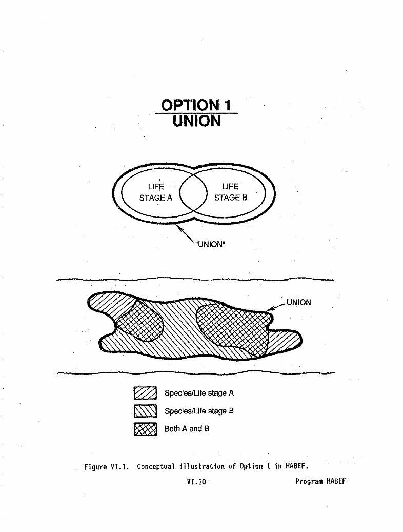
OPTION 1UNION
"UNION"
-------------------~ Species/life stage A
~ Species/life stage B
~ BothAandB
Figure VI.I. Conceptual illustration of Option 1 in HABEF.
VI.IO Program HABEF

DATE - 88/10/11. WILLIAMS FORK R[VER 8ELOW LEAH. COLORADO PROGRAM - HASEFTIME - 09.03.15. UNION ANALYSIS OF ADULT OROWN AND RAINOOW TROUT PAGE - 2
DATA SET 1 [5 DATA SET 2 [SCURVE HUMOER • 11102 CURVE NUMBER • 11302
SPECIES • RAINOOW TROUT SPECIES • aROWN TROUT
LIFE STAGE. ADULT L[FE STAGE' ADULT
RAIHOOWS SET ORDWNs SETTOTAL USAOLE AREA USABLE AREA UNION
DISCHARGE AREA USED WEIGHTED USED WEIGHTED wA
B.OO 7653.09 6849.35 606.95 2177 .00 912 .28 L246.55
15.00 8738.55 7937.63 960.76 2646.00 1336.09 1600.91
25.00 10142.23 9256.57 1375.67 3736.55 1620.19 2236.97
40.00 11578.09 10717 .16 1911.45 4826.55 1674.29 2616.40
GO.OO 13963.16 13036.93 2164.67 6536.35 1700.95 2164.60
60.00 15386.44 14486.54 2277.22 7474.05 1161.64 2919.50
100.00 16269.14 15338.07 2162.06 6016.60 1713.09 2662.27
125.00 17096.79 15368.41 1906.92 9394.60 1620.83 2645.85
150.00 10035.44 14273.86 1631. 74 10183.40 1606.24 2491.62
175.00 18837.04 13524.95 1499.27 10811.40 1633.98 2411.96
200.00 19036.68 12700.68 1381.59 11466.70 1601.41 2412.67
250.00 19334.14 10764.13 1103.26 13459.45 1559.76 2199.45
300.00 19376.56 8259.38 1050.24 14618.20 1562.36 2101.06
400.00 19450.99 5020.93 957.80 1136S.15 1530.64 1937.77
500.00 19512.23 4029.19 672.24 17953,70 1425.52 1768.46
750.00 19692.03 '2549.52 624.39 13767;52 1074.92 1329.74
1000.00 19808.23 1448.25 420.80 10061.05 842.60 IOU.55
END OF JOO
Figure VI.2. Sample output from HABEF when Option 1 is selected to obtain theunion of Brown and Rainbow Trout habitat space.
VI. 11 Program 11A6EF

WILLIAMS FORK RIVER BELOW LEAH, COLORAOOUNION ANALYSIS OF ADULT BROWN AND RAINBOW TROUTUNION OF AOUlT BROWN ANa RAINBOW TROUT
OISCHARGE RAINBOWS* 1 8.00* l 15.00* 3 25.00* 4 40.00*S 80.00, 6 60.00, 7 100.00* 6 125.00, 9 ·150.00*10 175.00*11 200.00*12 250.00*13 300.00'14 400.00*15 500.00*18 750.00*17 1000.00Ilt**_.,...*********
606.95960.76
1375.671911.452184.672277 .222182.081906.921651.741499.271587.591163.261050.24957.68872.24524.39420.80
BROWNS912.28
1338.091620.19.1674.291700.951751.841713.091620.631506.241633.961601.411559.761582.361530.641425.521074.92642;60
UNION1246.551600.912238.972616.402764.802919.502862.272645.652491.622477 .962412.672199.452101.061937.771768.461329.741023.65
Figure VI.3. The EHBl file written by HABEF when.Option 1 is selected.
VI.12 Program HABEF

COMPETITION ANALYSIS - Option 3
Of considerable interest Is the competition of two life stages or twospecies for the same space. An analysis of habitat competition can be doneusing Option 3 in HABEF.
The concept associated with competition analysis using Option 3 is shownin Figure VI.4. Most likely, two species will compete for some of the habitat,and in other places have the habitat all.to themselves (assuming two species arein the stream). In the competition habitat areas, there are places where onespecies/life stage is better sUited than the other; and other places where theconverse is true. Option 3 gives information on both of these possibilities asis illustrated in Figure VI.5.
Figure VI.6 contains the summary matrix table written to the HABEF outputfile when Option 3 is selected. The total Weighted Usable Area (WUA) is thesame as the WUA produced by HABTAT; the dominant WUA is ·the WUA which is usedby one species only, plUS the area subject to competition in which this speciesis dominant over the other. The summary results are also written to an EFTBLfile in a format similar to a ZHAQF file (Figure VI.7).
A comparison of the concepts of Option 1 and Option 3 is shown in FigureVI,8. These two options use the same information but do very differentanalyses. The two options compare the results from a HABTAT analysis for thesame streamflow. The file comparisons are shown in Figure VI.9.
VI.13 Program HABEF

OPTION 3COMPETITION ANALVSIS
Species 'compete" for this space
~ -~ Species/life stage A
~ Species/life stage B
m BolhAandB
Figure VI.4. Conceptual illustration of Option 3 in HABEF.
VI. 14 Program HABEF

DATE - 8B/l0/11.TI~ - OR.17.53.
WILLIAMS FORK RIVER BELOW tEAM. COLORADOCOMPETITION ANALYSIS OF BROWN TROUT WITH RAINBOW TROUT
PROGRAM • HABEFPAGE· 2
OATA SET 2 ISCURVE NUNBER' 11302
SPECIES • 8ROWN TROUT
liFE STAGE. AOULT
DATA SET I ISCURVE NUMBER = 11102
SPECIES • RAINBOW TROUT
LIFE STAGE' ADULT
OISCHARGE • 8.00 TOTAL AREA· 7G53.1SPECIES 1 ONLY- USABLE' 5267.4 WI. USABLE' 528.8SPECIES 2 ONLY- USABLE' 595.0 WI. USABLE. 284.1
BOTH SPEC1ES- USABLE. 1582.0WI. USABLE FOR 1 WITH 80TH- 278.3 WORTH FOR 1 GREATER THAN 2- 17.0WI. USABLE FOR 2 WITH BOTH- 828.2 WORTH FOR 2 GREATER THAN 1- 818.8SPECIES 1 OR 2 USABLE' 7444.4 EQUAL WORTH- 0.0
OISCHARGE • 15.00 TOTAL AREA = 8738.6SPECIES 1 ONLY- USABLE' 5747.6 WI. USA6LE' 442.5SPECIES 2 ONlY- USABLE' 858.0 WT.. USABLE. 331.1
BOTH SPECIES- USABLE' 2190.0WI. USABLE FOR 1 WITH BOTH- 51B.3 WORTH FOR 1 GREATER THAN 2- 47.9WI. USABLE FOR 2 WITH BOTH- 1007.0 WORTH FOR 2 GREATER THAN 1- 979.4SPECIES 1 OR 2 USABLE • 8595.6 EQUAL WORTH- 0.0
OISCHARGE • 25.00 TOTAL AREA· 10142.2SPECIES 1 ONLY- USABLE' 6243.0 WI. USABLE' 499.6SPECIES 2 ONLY' USA8LE • 721.0 WI. USABLE· 377.7
BOTH SPEC[ES- USABLE = 3015.BWI. USABLE FOR 1 WITH BOTH- 878.0 WORTH FOR I GREATER THAN 2- 430.3WI. USABLE FOR 2 WITH BOTN- 1242.5 WORTH fOR 2 GREATER THAN 1- 931.4SPECIES 1 OR 2 USA8LE • '9979.8 EQUAL WORTH- 0.0
OISCHARGE • 40.00 TOTAL AREA = 11578.1SPECIES 1 ONLY- USABLE. 6611.6 WI. USA8LE = 515.7SPECIES 2 ONLY- USABLE = 721.0 WT. USABLE. 430.7
80TH SPECIES- USABLE' 4105.5WI. USABLE FOR [ WITH BOTH- 1395.8 WORTH FOR 1 GREATER THAN 2- 882.7WI. USABLE FOR 2 WITH 80TH- 1243.5 WORTH FOR 2 GREATER THAN 1- 787.4SPECIES 1 OR 2 USABLE = 11438.2 EQUAL WORTH- 0.0
DISCHARGE. 60.00 TOTAL AREA· 13963.2SPECIES 1 ONLY- USABLE' 7282.4 WI. USABLE = 484.5SPECIES 2 ONlY- USABLE' 781.B WI. USA6LE = 444;8
BOTH SPECIES- USABLE· 5756.5WI. USABLE FOR I WITH BOTH- 1700.1 WORTH FOR 1 GREATER THAN 2- 1241.0Yr. USABLE FOR 2 WITH SOTH- 1258.2 WORTH FOR 2 GREATER THAN 1- 594.5SPEC [ES I OIl 2 USA6LE • 13820.7 EQUAL WORTH- 0.0
Figure VI.5. Sample output from HABEF when Option 3 is selected.
VI.15 Program HABEF

DATE - 88/10/11.TlHE - 09.17.53.
WILLIAM5 FORK RIVER 8ELOW LEAH, COLORAOOCOHPETlTIOJl AMALYSIS OF BROWN TROUT WITH RAINOOW TROUT
SUHNARY OF COHPETITION'ANALYSIS-
PROGRAH - HA8EFPAGE - 5
TOTAL WUA OOHINATE WUADISCHARGE RAIHBOWS BRowns RAINBOWS BRowNS
8.00 606.93 912.28 345.65 900.8715.00 960.76 1338.09 490.45 1310.4525.00 1375.63 1620.19 929.87 1309.0540.00 1911.45 1874.20 1398.87 1218.0360.00 2184.64 1700.95 1725.51 1039.2580.00 ZZ77.Z2 1761.84 1819.29 1100.21
100.00 2182.08 1713.09 1767.78 1094.49125.00 1905.92 1820'B2 1582.11 1083.74150.00 1531. 50 1505.24 1332·75 1158.84175.00 1499.22 1633.98 1149.22 1328.71200.00 1387.59 1601.41 ' 1061.31 1351.35250.00 1183.26 1559.76 889.54 1309.90300.00 1050.22 15B2.36 756.87 1344.19400.00 957.88 1530.50 675.05 12e2.67500.00 872.18 1425.52 B14.70 1153.76750.00 624.39 1074.86 441.77 B87.90
1000.00 420.80 842.73 299.26 724.32END OF JOB
Figure VI.S. Summary table written to output file by HABEF when Option 3 isselected.
VI.16 Program HABEF

BROWNS900.87
1310.451309.061216,031039.26
. 1100.211094.491083.74\156.84 .1328.711351.351309.901344.191262.871153,76687.90724,32
WILliAMS FORK RIVER BELOlI LEAH. COlORAOOCOMPETITION ANALYSIS OF BROWN TROUT WITH RAINBOlI TROUTCOMPETITION ANALYSIS - TOTAL THEN DOMINATE
OISC~R6E RAINBOWS BROWNS RAINBOlIS* I 8.00 606.93 912.28 345.65* 2 15.00 960.78 1338.09 490.45* 3 25.00 1375.63 1620.19 929.87* 4 40.00 1911.45 1874.20 1398.37* 5 60.00 2184.64 1700.95 1725.51* 6 80.00 2277,22 1781,84 1819.29* 7 100.00 2162.06 1713.09 1767.78* 8 125.00 1906,92 1620.82 15B2.11* 9 150.00 1631.60 1606.24 1332.75*10 175.00 1499.22 1633.98 1149.22*11 200.00 1387.59 1601.41 1061.31*12 250.00 1183.26 1559.76 689.54*13 300.00 1050,22 1582.36 756.87*14 400.00 957,88 1530.60 675.06*15 500.00 672.18 1425.52 614.70*18 750.00 624.39 1074.86 441.77*17 1000.00 420.80 842.73 299.26**,,"****_*****1"'"
Figure VI.7. The EFTBl file written by HABEF when Option 3 is selected.
\11.17 Program HABEF
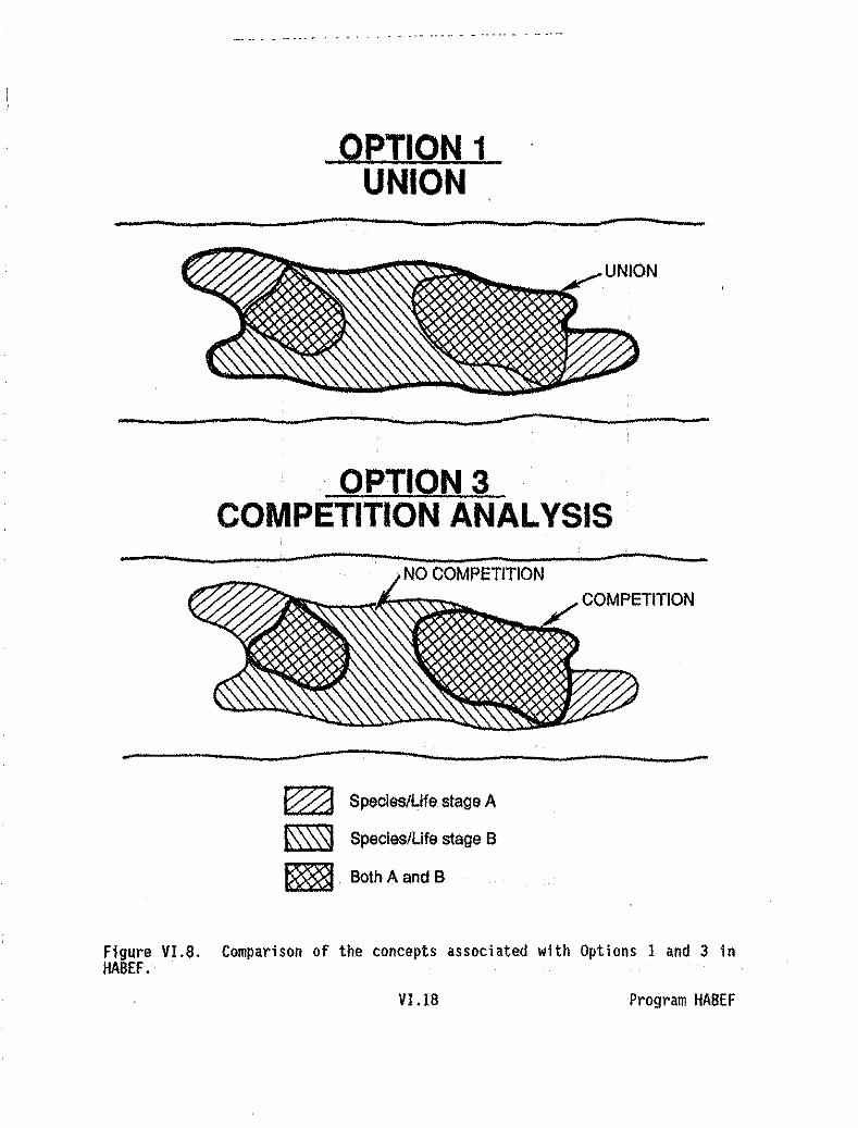
·_--_._-_.... -- -_.
OPTION 1UNION
----------------------OPTION 3
COMPETITION ANALYSIS
.NO COMPETITION
~ -~ SpecieS/Ufe stage A
~ Species/Life stage B
~ BothAandB
Figure VI.8. Comparison of the concepts associated with Options 1 and 3 1nHABEF.
VI.I8 Program HABEF

ZHCF(1) ZHCF(2)
Q 1,1 Q 2,1
.
Q 1,2 Q2,2
Q 1,3 Q 2,3
Q1,4 Q2,4..
Q 1.5 Q2,5
Q11=Q2i, t
OPTIONS 1, 3
OPTIONS 5, 6
Same number of flows on each file.
figure VI.9. file comparisons when Option I, 3, 5, or 6 is selected in HABEF.
VI. 19 Program HABEF

MAXIMUM/MINIMUM ANALysES - Options 5 and 6
The purpose of Options 5 and 6 is to compare the state under one condition(flow, species, etc.) for a specific cell to the state with a second conditionin the same cell. This file comparison process is illustrated in Figure VI.9.
There are two logics used in the comparison.
The logic for Option 5 is:
WUA = HIN(WUA(1),WUA(2»
where WUA(l) is the composite suitability factor from the first file, andWUA(2)is the composite suitability factor from the second file.
The logic for Option 6 is:
WUA·= HAX(WUA(ll,WUA(2l)
Figure VI.IO contains the results for Option 5. Figure VI.ll contains theresults for Option 6.
An EFTBl file which is similar to a ZHAQF file is also produced (FigureVI.I2l. The first column contains the WUA for the first file, the second columncontains the WUA for the second file, and the third column contains the minimumor maximum WUA depending on the option selected. The discharge written is fromthe first file; if the discharge on the second file is different from the first,it is written in the fifth column.
VI.20 Program HABEF

DATE· 88/10/11. WILLIAMS FORK RIVER BELOW LEAH. COLORADO PRDORAIl . HABEFTIME' OR.2B.55. MINIMUM HABITAT AHALYSISWITH BASE FLOW OF 8 CF5 PAGE - 2
DATA SET lIS DATA SET 2 ISCURVE NUMBER • lIl02 CURVE NUMBER • 11102
SPECIES = RAINBOW TROUT SPECIES =RAINBOW TROUT
LIFE STAGE = ADULT LIfE STAGE =ADULT
MINIMUM Q SET BASE Q SETTOTAL USABLE AREA TOTAL USABLE AREA
MINIMUMDISCHARGE AREA USED WEIGHTED DISCHARGE AREA USED II£IGHTED WUA
8.0 7653.1 6849.4 605.9 8.0 7553.1 6849.4 605.9 506.9
15.0 8138.5 7937.6 960.8 15.0 8738.6 7937.6 950.8 980.8
25.0 10142.2 92S8.6 1375.1 25.0 10142.2 9258.6 1375.7 1375.7
40.0 11518.1 10717.2 19I1.4 40.0 11578.1 10117.2 1911.4 1911.4
60.0 13983.2 13038.9 2184.7 60.0 13963.2 13038.9 2164.1 2184.1
80.0 15386.4 14466.5 2271.2 80.0 15385.4 14486.6 n71.2 2277.2
100.0 16289.1 15338.1 2182.1 100.0 16289.1 15338.1 2182.1 2182.1
125.0 17096.8 15388.5 1906.9 12~.0 17095.8 15388.5 1906.9 1906.9
150.0 18035.4 14273.9 1631.1 150.0 18035.4 14273.9 1631. 7 1631.7
175.0 16837.8 13525.0 1499.3 175.0 18837.8 13525.0 1499.3 1499.3
200.0 19036.7. 12700.7 1387.6 200.0 19036.7 12700.7 1387.5 1387.5
250.0 19334.1 10764.1 H83.3 250.0 19334.1 10764.1 1163.3 HB3.3
300.0 19376.6 6.259.4 1050.2 300.0 19376.6 8259:4 1050.2 1050.2
400.0 19451.0 5020.9 957.9 400.0 19451.0 . 5020.9 957.9 957.9
500.0 19512.2 4029.2 872.2 500.0 19512.2 4029.2 812.2 872.2
750.0 19692.0 2649.5 624.4 150.0 19692.0 2049.5 624.4 524.4
1000.0 19808.2 1448.2 420.8 1000.0 19B08.2 1448.2 420.8 420.8
END Of J08
Figure VI.IO Sample output from HABEF when Option 5 is selected.
VI.21 Program HABEF
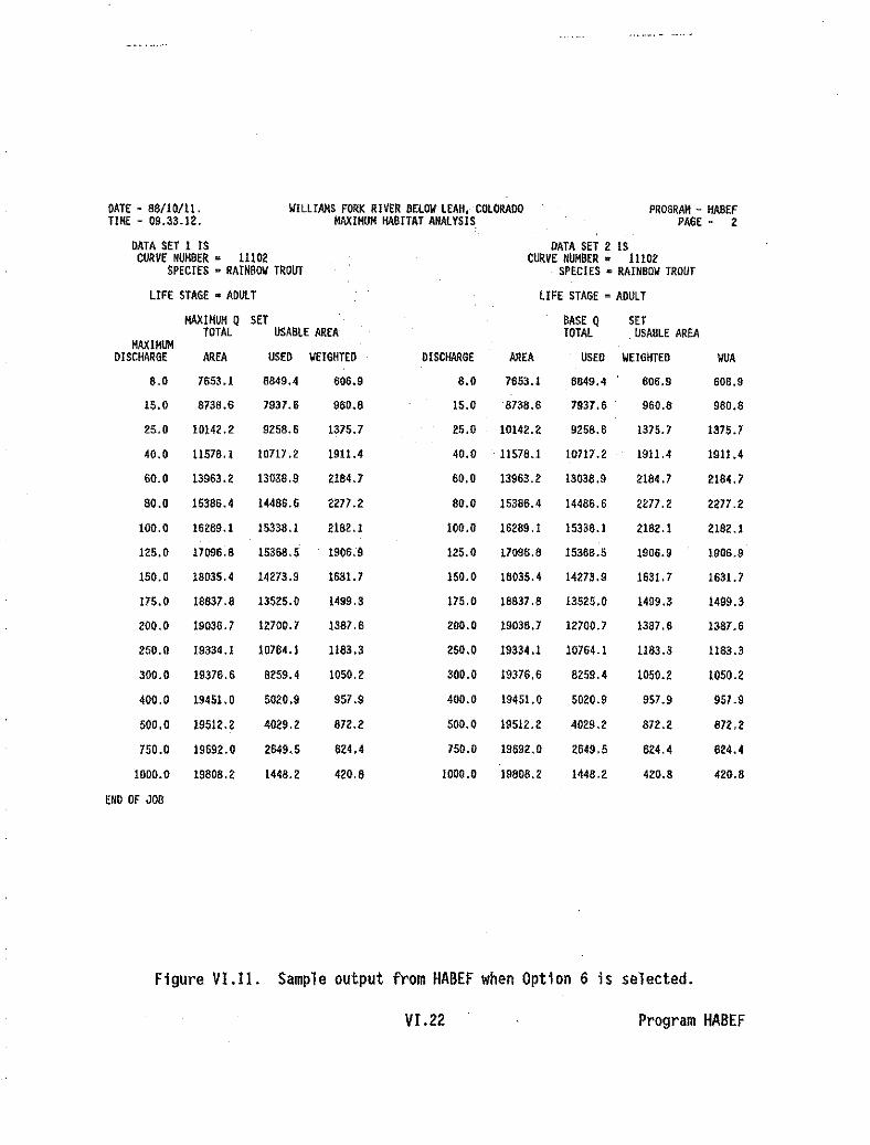
OATE - 88/10/11. WILllAllS FOilK RIVER SEl.O\I LEAH. COLORADO PROGRAM - HASEFWIl: - 09.33.12. MAXIMUM HABITAT ANALYSIS PAGE - 2
DATA SET 1 IS DATA SET 2 ISCURVE NUMBER • 11102 CURVE NUMBER • JIlD2
SPECIES • RAINBOW TROUT SPECIES • RAINBOW TROUT
LIFE STAGE. ADULT LIFE STAGE' ADULT
MAXIMUM Q SET BASE Q SETTOTAL USABLE AREA TOTAL USABLE AREA
MAXIMUMDISCHARGE AREA USED WEIGMTEO DISCHARGE AREA USED WEIGMTED WUA
8.0 7653.1 6849.4 606.9 8.0 7653.1 8849.4 606.9 606.9
IS.0 8736.6 7937.6 960.8 15.0 8738.6 7837.6 960.8 980.8
25.0 10142.2 9268.8 1375.7 25.0 10142.2 9258.6 1375.7 1375.7
40.0 11578.1 10717.2 1911.4 40.0 11578.1 10717.2 1911 .4 1911.4
60.0 13963.2 13038.9 2184.7 60.0 13963.2 13038.9 2184.7 2184.7
80.0 15386.4 14486.6 2277.2 80.0 15386.4 14486.6 2277.2 2277 .2
100.0 16289.1 15338.1 2182.1 100.0 16289.1 15338.1 2182.1 2182.1
125.0 17096.8 1536B.5 190B.9 125.0 1709B.8 153B8.5 1906.9 1906.9
150.0 18035.4 14273.9 1631. 7 150.0 18035.4 14273.9 1631.7 1631. 7
175.0 18837.8 13525.0 1499.3 175.0 18837.B 13525.0 1499.3 1499.3
200.0 19036.7 12700.7 1387.6 200.0 19036.7 12700.7 1387.6 1387.6
250.0 19334.1 10764.1 1183.3 250.0 19334.1 10764.1 1183.3 1183.3
300.0 19378.6 8259.4 1050.2 300.0 19376.6 8259.4 1050.2 1050.2
400.0 19451.0 5020.9 957.9 400.0 19451.0 5020.9 957.9 957.9
500.0 19512.2 4029.2 872.2 500.0 19512.2 4029.2 872.2 872.2
750.0 19692.0 2649.5 824.4 750.0 19692.0 2649.5 624.4 624.4
1000.0 19808.2 1448.2 420.8 1000.0 19808.2 1448.2 420.8 420.8
ENO OF J08
Figure VI.II. Sample output from HABEF when Option 6 is selected.
VI.22 Program HABEF

WILLIAMS fORK RIVER 8ELOW LE~H. COLORAooMAXIMUM HA81T~T ~H/ll.YSIS
ADULT RAINBOW TROUT WITH BASE Q Of 8 CfSDISCHARGE MAXIMUM Q BASE Q
• 1 8.00 606.95 606.95• 2 15.00 960.78 960.78• 3 25.00 1375.67 1375.67• 4 40.00 1911.45 1911.45• 5 60.00 2184.67 2184.67• 6 80.00 2277.22 2277.22• 7 100.00 2182.08 2182.08" 8 125.00 1906.92 1906.92* 9 150.00 1631.74 1631.74*10 175.00 1499.27 1499.27*11 200.00 1387.59 1387.59*12 250.00 1183.26 1183.26"13 300.00 1050.24 1050.24*14 400.00 957.88 957.88"IS 500.00 872.24 872.24*16 750.00 624.39 624.39*17 1000.00 420.80 420.80***************
MAXIMUM 2ND DISCH.606.95980.78
1375.671911.452184.672277 .222162.081908.921631.741499.271387.591183.261050.24957.88872.24624.39420.80
Figure VI.12. The EHBL file written by HABEF when Optipn 6 is selecteci.
VI.23 Prpgram HABEF

• _, • _e • ." ••
STREAMFLOW VABIATION ANAlYSIS - Option 2, 4, 7, or 8
The purpose of the streamflow variation analysis is to look at the habitatfrom two flows with both flows varying over a range. Tile analysis is similarto the maximum/minimum analysis with the difference being that all flow sets onone file are compared to all flow sets on another file. Effective spawninglogic can also be done. In effective spawning analysis, an area available forspawning habitat is available only if the incubation is satisfactory during thefollowing incubation period.
This type of comparison of flows is demonstrated in Figure VI.13.
Option 2 is where WUA a HIN(WUA{l,i),~UA(2,k»
Option 4 is where WUA • HAX(WUA(1,i),WUA(2,k»
Option 7 is 1F(WUA(2) > 0
IF(WUA(2) • 0
Option 8 is IF(WUA(2) > 0
IF(WUA(2) ~ 0
WUAE ~ WUA0)
WUAE • 0.0
WUA£ = WUA(1)
WUAE = 0.0
( XWUAE J *S1 ~ 1.0· ZWUA{l) 100.0
The output resulting from Option 2 is illustrated in Figure VI.I4. Theresults from Option 4 will look the same, except that the last column will bethe maximum value of the combined habitat instead of the minimum.
The last page of the output is a matrix table of the results of theanalysis as shown in Figure VI.IS. The summary output Is also written to theEFTBl file (two-flow habitat file when Option 2, 4, 7 or 8 Is selected) in aform that can be used In Time Series analysis. A portion of this file ispresented in Figure V1.I6.
Effective spawning analysis is done If Option 7 Is selected. The logicbehind effective spawning Is illustrated In Figure VI.17. The results obtainedwhen Option 7 Is used are shown in Figure VI.la.
Stranding index analysis is done if Option 8 is selected. The logicbehind stranding index analysis is illustrated in Figure VI.19. The resultsobtaining when Option 8 is used are shown in Figure VI.20.
VI.24 Program HABEF
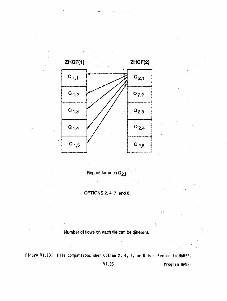
ZHCF(1) ZHCF(2)
o i,i 02,1
01,2 02,2
01,3 02.3
01,4 02,4
01,5 02,5
Repeat for each 02,i
OPTIONS 2, 4, 7, and 8
Number of flows on each file can be different.
Figure VI.13. File comparisons when Option Z, 4, 7, or 8 is selected in HABEF.
Vl.25 Program HABEF

DATE' 88/10/11. VILLlAMS rOflK RIVER BELOII LEAH. COLOflAOO PROGRAM • HABErTlHE· 11.53.12. MINIHUM VARIATION ANALYSIS PAGE· . 2
FIRST DATA SET IS SECOND DATA SET ISCURVE NUMBER • 11102 CURVE NUMBER • 11102
SPECIES • RAINBOW TROUT SPECIES =RAIHBO\I TROUT
LirE STAGE. ADULT LIFE STAGE. ADUlT
FIRST SET SECOND SETTOTAL USABLE AREA TOTAL USAllLE AREA
HINIHUHDISCHARGE AREA USED WEIGHTED DISCHARGE AREA USED WEIGHTED WUA
8,0 7653.1 6849.4 606.9 B.O 7653.1 6B49.4 606.9 606.915.0 6736.6 7937.6 960.B 8.0 7653.1 6849.4 606.9 605.625,0 10142.2 9256.6 1375.7 6.0 7653.1 6849.4 606.9 599.940.0 11578.1 10717.2 1911.4 8.0 7653.1 6849.4 606,9 584.560.0 13963.2 13038.9 2184.7 8.0 76S3.l 6849.4 606.9 554.080.0 15386.4 14486.6 2277 .2 8.0 7653. I 6849.4 608.9 530.6
100.0 16289.1 15338.1 2182.1 8.0 7653.1 6849.4 606.9 470.3125.0 11096.6 15388.5 1908.9 8.0 7653.1 6849.4 606.9 371.7150.0 18035.4 14213.9 1631.1. 8.0 1653.1 8649.4 608,9 251.5115.0 18831.8 13525.0 1499.3 6.0 1653.1 6849.4 '608.9 112.6200.0 19036.1 12700.1 1381.6 6.0 1653.1 6849.4 608.9 112.8250.0 19334.1 10764.1 1183.3 8.0 7653.1 6849.4 806.9 67.0300,0 19375.6 6259.4 1050.2 8.0 7653.1 6849.4 606.9 59.9 .400.0 19451.0 5020.9 957.9 8.0 1653.1 6849.4 608.9 52.3500.0 19512.2 4029.2 812.2 8.0 7653.1 6849.4 606.9 33.1150.0 19692.0 2649.5 824.4 8.0 1853.1 6849.4 806.9 .12.8
1000.0 19808.2 1448.2 420.8 8.0 7653.1 6849.4 606.9 06.2
8.0 1853.1 6849.4 608.9 15.0 8136.6 1931.8 960.8 605.615.0 8138.6 1931.6 960.8 15.0 8138.6 1937.6 980.8 960.825.0 10142.2 9258.8 1375.1 15.0 8138.6 7937.6 960.8 948.540.0 11578.1 10117.2 1911.4 15.0 8738.6 1931.6 960.8 924.060.0 13963.2 13038.9 2184.7 15.0 8738.6 7931.6 960.8 880.180.0 15386.4 14486.6 2277 .2 15.0 8138.6 7931.6 960.8 801.8
100.0 18289.1 15338.1 H82.l 15.0 8738.6 7931.6 980.8 899.8125.0 17096.8 15388.5 1908.9 15.0 6738.6 1931.6 980.8 538.8150.0 18035.4 14273.9 1631.1 15.0 8136.8 1931.6 980.6 369.2115.0 16837.8 13525.0 1499.3 15.0 8138.8 7931.6 960.8 253.0200.0 19038;7 12100.1 1387.6 15.0 8138.8 7931.6 980.6 169.2250.0 19334.1 10184.1 1183.3 15.0 8738.6 7937.8 960,8 113.4300.0 19316.6 8259.4 1050.2 15.0 6138.6 7937.6 960.8 94.0400.0 19451.0 5020.9 951.9 15.0 8738.6 1931.6 960.8 16.9500.0 19512.2 4029,2 672.2 15.0 8738.6 1937.6 960.8 48.6150,0 19692.0 2649.5 624.4 15.0 8138.6 1937.6 980.8 15.2
1000.0 19808.2 1448.2 420.8 15.0 8738.6 1937.6 980.8 08.6
Figure VI.14. Sample output from HABEF when Option 2 is selected.
VI.26 Program HABEF

DAT. - 88/10/11.TINE - 11.53.12.
WILL III"S FORK RIVER BELOII LEII", COLORADONININUlI VAlUATION II"ALYSIS
PRGGRII" - HAGEFPAGE· .11
NININUlI VARIATION ANALYSIS - ADULT RAINGOII TROUT
SECOND FLOWSFIRSTFLOIIS
8.0 15.0 25.0 40.0 60.0 80.0 100,0 125.0 150.0 175.0 200,0
!~~-------~------~~~---------._-----------------------------------------~----------------~---------I
8.0 I 606.9 605.6 599.9 584.5 554.0 530.6 470.3 371.7 251.5 172,8 112,8!
15,0! 605.6 960,8 946.5 924,0 880.1 807.8 699,8 536.6 369.2 253,0 169.2I
25.0 I 599.9 946.5 1375.7 1343,5 1260.0 1129.5 959.1 750.2 494.7 351.6 247.9I
40,0! 584,5 924.0 1343.5 1911.4 1750.0 1558.0 1326.2 991.5 669,0 472.0 354.6I
60.0 I 554,0 880.1 1260.0 1750.0 2184.7 1953,0 1695.2 1285.9 903,1 671.2 525.2I
80.0 I 530.8 807.8 1129.5 1558.0 1953.0 2277,2 1977,2 1517,0 1109,5 854,7 678,5I
100,0 I 470.3 699,8 959,1 1326.2 1695.2 1971.2 2182,1 1707.0 1282,3 1013.1· 824.3!
125.0 1 371.7 538.6 750,2 991,5 1285,9 1517.0 1707.0 1906.9 1463.9 1182.1 977.31
150.0 I 251.5 369.2 494,7 669,0 903.1 1109.5 1262.3 1463.9 1631.7 1341.7 1124.1I
175.0 ! 172.8 253.0 351.6 472.0 871.2 854.7 1013.1 1182.1 1341.7 1499.3 1278.3I
200.0 I 112.8 169.2 247,9 354,6 525.2 678.5 824.3 977.3 1124.1 1278.3 1387.6I
250.0! 67,0 113,4 176,0 267,9 388,9 499.7 606,1 728.2 841,8 968,7 1058.0!
300,0 I 59.9 94.0 143.2 209.3 304.1 390.8 471.2 561.6 652.1 744.2 808.3I
400.0 ! 52.3 76.9 113.7 155,1 214.4 274.8 323.7 380.2 436.4 483.9 536.2I
500.0 I 33.1 48.6 69;3 102,6 155.3 191.4 234.5 276,8 320.9 362.8 406.6I
750.0 I 12.6 15.2 23.4 47.4 92.9 126,9 148.8 115.7 202,4 221.9 255.4I
10oo.0! 6.2 6,6 15.1 33.9 66.0 81.3 90.1 100.7 113.2 125.6 137,8
Figure VI.IS. Summary table written to output file by HABEF when Option 2 isselected.
VI.27 Program HABEF

DATE - 88/10/11.TIME - 11.53.12.
WILLIAMS FORK RIVER BELOV LEAH. COLORADOMINIMUM VARIATION ANALYSIS
MINIMUM VARIATION ANALYSIS • ADULT RAINBDV TROUT
PROGRAM - HABEFPAGE - 12
FIRSTFLOWS
250.0 300.0
SECOND
400.0
nM
500.0 750.0 1000.0
1---------------------------------------------------------------,8.0 , 67.0 55.9 52.3 33.1 12.8 6.2
!15.0 I 113.4 94.0 76.9 48.6 IS.2 8.6
t25.0 I 176.0 143.2 113.7 69.3 23.4 15.7
I40.0 ! 257.9 209.3 155.1 102.6. 47.4 33.9
I60.0 , 388.9 304.1 214.4 155.3 52.9 68.0,80.0 , 499.7 390.8 274.B 197.4 126.9 81.3
I100.0 ! 606.1 471.2 323.7 234.5 148.8 90.7
I125.0 ! 728.2 561.6 380.2 276.8 175.7 100.7
1150.0 I 641.8 652.1 436.4 320.9 202.4 113.2
I175.0 I 568.7 744.2 463.5 362.8 227.9 125.8
I200.0 I 1056.0 B06.3 536.2 406.B 255.4 137.8
1250.0 1 1183.3 926.5 640.2 503.2 305.3 160.4
1300.0 I 926.5 1050.2 755.9 611.3 352.4 188.2
I400.0 I 640.2 755.5 957.9 777.2 442.6 252.7
I500.0 ! 503.2 611.3 777.2 872.2 495.5 293.1,750.0 I 305.3 352.4 442.6 495.5 524.4 382.1
11000.0 I 160.4 188.2 252.7 293.1 382.1 420.8
Figure VI.15. (Concluded)
VI.2S Program HABEF

VIlLlAMS FORK RIVER BRO\/ lEAH, COlORADOMINIMUM VARIATION AHAlVSISFIRST - SECONO TABlEMINIMUM VARIATION ANALYSIS - AOULT RAINBOW TROUT
17 17B.OO
15.0025.00~O.OO
60.00BO.OO
100.00125.00150.00175.00ZOO.OOZ50,OO300.00~OO.OO
500.00750.00
1000.008.00
15.0025,00~O.OO
60.00BO.OO
100.00125.00150.00175.00200.DO250.00300.00400.00500.00750.00
1000.00606.95605.56599,89584.51554.04530.56
SAMPLE OUTPUT TERMINATED FOR BREVITY.
Figure VI.16. The EFTBL file written by HABEF wben Option 2, 4, 7, or 8 isselected.
III. 29 Program HABEF
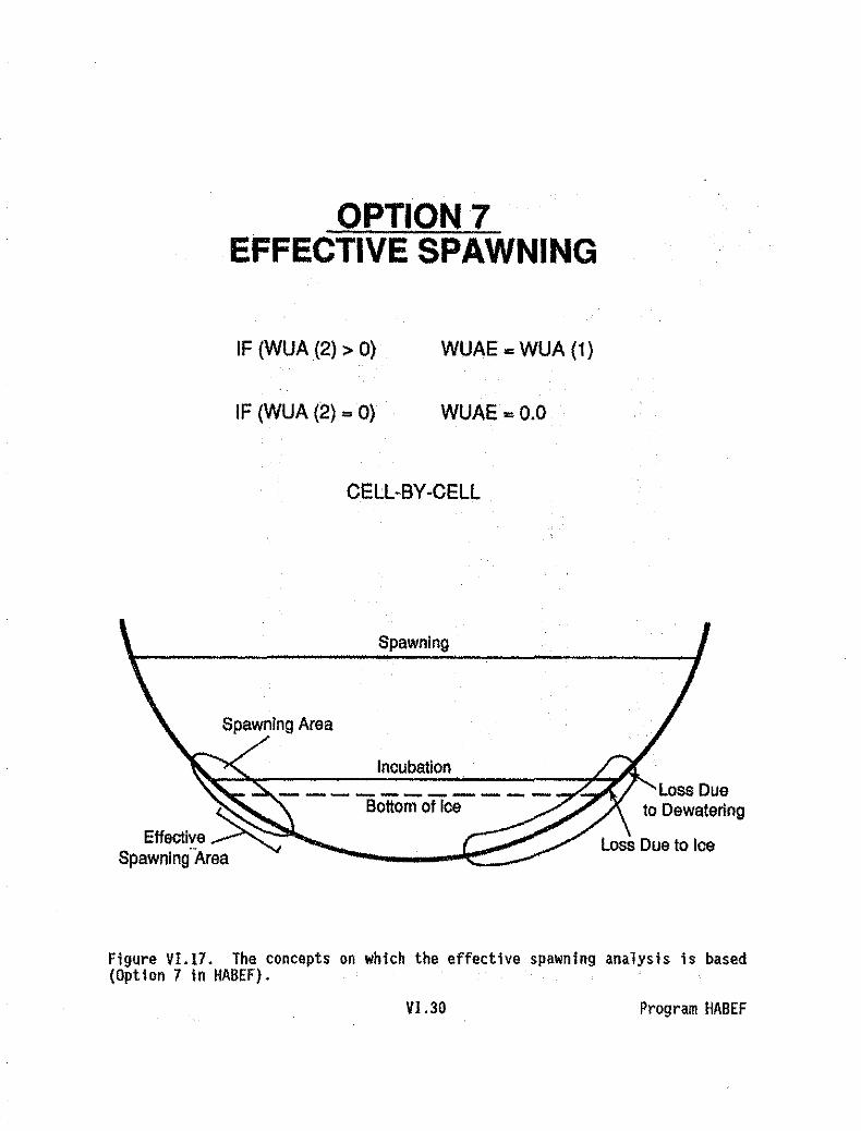
OPTION 7EFFECTIVE SPAWNING
IF (WUA (2) > 0)
IF (WUA (2) ... 0)
WUAE ... WUA (1)
WUAE=O.O
CELL-BY·CELL
Spawning
IncubationLoss Due
to Dewatering
Figure VI.I7. The concepts on which the effective spawning analysis is based(Option 7 in HABEF).
VI.30 Program HABEF

DATE - 88/10/11. WILLIAMS FORK RIVER BELOW. LEAH, COLORADO PROGRAM - HA8EFTIME - 10.01.35. EffECTIVE SPAWNING ANALYSIS PAGE - 2
SPAWNING DATA SET IS INCUBATION DATA SET ISCURVE NUMBER • 11110 CURVE NUM8ER • 30001
SPECIES • RAINBOW TROUT SPECIES • SALMDNIDAE (SALMON/TROUT)
LIfE STAGE = LIFE STAGE =
SPAWNING INCUBATION TOTAL ORIGINAL EFfECTIVEOISCHARGE DISCHARGE AREA SPAWNTNG AREA SPAWNING AREA
8.00 8.00 7663.09 98.53 0.0016.00 8.00 8738.66 321.85 6.4025.00 8.00 10142.23 817.26 23.9640.00 B.OO 11578.09 1442.16 29.5660.00 8.00 13963.16 1830.33 23.9880.00 8.00 15386.44 1912.02 15.81
100.00 8.00 18289.14 1887.84 8.68125.00 8.00 17096.79 1839.81 3.75150.00 ?OO 18035.44 1895.99 1.29175.00 8.00 18837.84 1892.33 0.11200.00 B.OO 19038.68 1B56.24 0.00250.00 8.00 19334.14 1880.04 0.00300.00 8.00 19378.58 . 1407.48 0.00400.00 8.00 19450.99 1040.64 0.00500.00 6.00 19512.23 935.29 0.00750.00 B.OO 19692.03 281.93 0.00
1000.00 B.OO 19808.23 49.81 0.00
8.00 15.00 7653.09 96.53 0.0015.00 15.00 8738.55 321.85 6.4025.00 15.00 10142.23 817.26 37.3540.00 15.00 1157B.09 1442.16 49.7660.00 15.00 13963.16 1830.33 48.6980.00 15.00 15386.44 1912.02 35.11
100.00 15.00 16289.14 18B7.84 23.71125.00 15.00 17096.79 1839.61 12.24150.00 15.00 lB035.44 1895.99 6.3B175.00 15.00 18637.84 1892.33 2.93200.00 15.00 19036.6B 1856.24 1.00260.00 15.00 19334.14 16BO.04 0.09300.00 15.00 19376.58 1407.4B 0.00400.00 15.00 19450.99 1040.64 0.00500.00 15.00 19512.23 935.29 0.00760.00 15.00 19892.03 281.93 0.00
1000.00 15.00 19808.23 49.B1 0.00
Figure VI.IB. Sample output from HABEF when Option 7 is selected.
VI.31 Program HABEF

QPTJQN8STRANDING INDEX
IF (WUA (2) > 0)
IF (WUA (2) "" 0)
WUAE .. WUA (1)
WUAE .. 0.0
CELL-BY-CELL
~WUAE ) * 100.0~WUA(1} .
Figure VI.19. The concepts on which the stranding index analysis Is based(Option 8 in HABEF).
VI.32 Program HABH
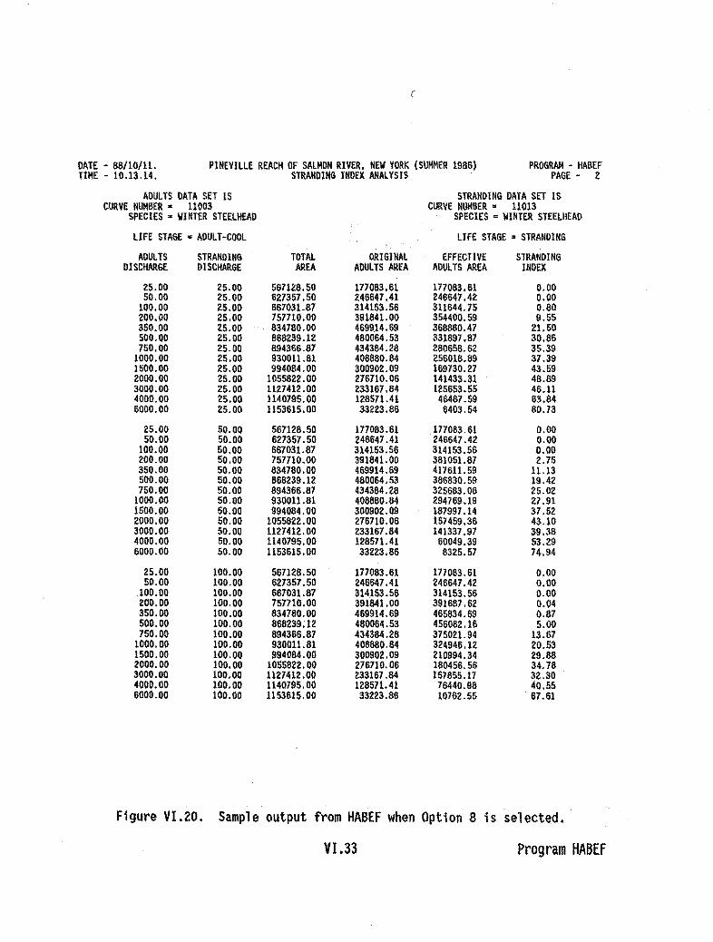
(
DATE - 88/10/11. PINEVILLE REACH OF SALHDN RIVER. NEW YORK (SUMMER 1986) PROGRAM • HA8EFTIME - 10.13.14. STRANDING INDEX ANALYSIS PAGE - 2
ADULTS DATA SET IS STRANDING DATA SET ISCURVE NlIMBER • 11003 CURVE NUM8ER • 11013
SPECIES • WINTER STEELHEAD SPECIES =WINTER STEELHEAD
liFE STAGE· ADULT-COOL LIFE STAGE • STRANDING
ADULTS STRANDING TOTAL ORIGINAL EFFECTIVE STRANDINGOISCHANGE DISCHANGE AREA ADULTS AREA AOULTS AREA INDEX
25.00 25.00 567128.50 177083.61 177083.61 0.0050.00 25.00 627357.50 246647.41 246647.42 0.00
100.00 25.00 667031.87 314163.56 311644.75 0.60200.00 25.00 757710.00 391641.00 354400.59 9.55350.00 25.00 634780.00 4699.14.69 368560.47 21.50500.00 25.00 868239.12 480064.53 331897.87 30.86750.00 25.00 894366.87 434364.26 280658.62 35.39
1000.00 25.00 930011.81 408e80.64 256018.89 37.391500.00 25.00 994084.00 300902.09 169730.27 43.592000.00 25.00 1055822.00 276710.06 141433.31 48.893000.00 25.00 1121412.00 233167.84 125653.55 46.114000.00 25.00 1140795.00 128571.41 46487.59 63.846000.00 25.00 1153615.00 33223.86 6403.54 80.73
25.00 50.00 567128.50 177083.61 177063.61 0.0050.00 50.00 627357.50 246647.41 246647.42 0.00
100.00 50.00 667031.87 314153.56 314153.56 0.00200.00 50.00 757710.00 391641.00 381051.87 2.75350.00 50.00 834780.00 468914.69 417611.59 11.13500.00 50.00 888239.12 480064.53 386830.59 19.42750.00 50.00 894366.87 434384.28 325683.06 25.02
1000.00 50.00 930011.81 408880.84 294769.19 27.911500.00 50.00 994084.00 300902.09 187997.14 37.522000.00 50.00 1055822.00 276710.08 157459.38 43.103000.00 50.00 1127412.00 233167.84 141337.97 39.384000.00 50.00 1140795.00 128571.41 60049.39 53.296000.00 50.00 1153615.00 33223.86 8325.57 74.94
25.00 100.00 567128.50 177083.61 177083.61 0.0050.00 100.00 627357.50 246647.41 246647.42 0.00
100.00 100.00 667031.67 314153.56 314153.56 0.00200.00 100.00 757710.00 391641.00 391667.62 0.04350.00 100.00 834760.00 469914.69 465834.69 0.87500.00 100.00 668239.12 480064.53 456082.16 5.00750.00 100.00 894366.87 43431lol.28 375021.94 13.67
1000.00 100.00 930011.81 408880.84 324946.12 20.531500.00 100.00 994084.00 300902.09 210994.34 29.682000.00 100.00 1055822.00 276710.06 160456.56 34.783000.00 100.00 1127412.00 233167.84 157655.17 32.304000.00 100.00 1140795.00 128571.41 76440.98 40.556000.00 100.00 1153615.00 33223.68 10762.55 87.61
Figure VIo20. Sample output from HABEF when Option 8 is selected..
VI.33 Program HABEF

lSTCEl Program
I. INTRODUCTION
The lSTCEl program lists the contents of a ZHCF file and uses a TAPE3 filecontaining unformatted cross section and reach data that was generated by thehydraulic simulation programs.
The output from lSTCEl is a listing of the composite sUitability of usefactors in a format that makes it easy to see how the composite suitability ofuse terms vary across the stream channel and as a function of discharge. Theoutput resembles a "map" if the cell widths are nearly the same across a crosssection. '
II. RUNNING lSTCEl
lSTCEL,ZHCF,TAPE3,ZOUT ,
ZHCF~unformatted cell areas and cell weighted usaple areas (input)TAPE3~unformatted cross section and reach data (input)ZOUT=LSTCEl results (output)
Figure VI.2l contains sample output from the LSTCEl program.
VI.34 Program lSTCEl

88/10/11. WILLIAMS FORK RIVER SECTIOM 1 •• COlORAOO/MEHRING •• PROGRAM - lSTCEl10.24.04. ONE MILE BELOW KIMNEY CREEK CONFLUENCE IFG4 DATA PAGE· 2
RAINBOW TROUT liFE STAGE - ADUlT HUMBER - 11102 STATION· 0.00
DISCHARGEX Y S 8.0 1,.0 25.0 40.0 60.0 80.0 100.0 125.0 150.0 175.0 200.0 2'0.0
1 1.0 98.60 4.00 0.00 0.00 0.00 0.00 0.00 0.00 0.00 0.00 0.00 0.00 0.00 0.002 2.0 98.50 4.00 0.00 0.00 0.00 0.00 0.00 0.00 0.00 0.00 0.00 0.00 0.00 0.003 4.0 96.30 4.00 0.00 0.00 0.01 0.02 0.04 0.05 0.06 0.07 0.07 0.08 0.09 0.114 6.0 96.20 ,.50 0.00 0.01 0.04 0.07 0.10 0.14 0.16 0.16 0.16 0.15 0.15 0.155 B.O 96.10 5.50 0.00 0.02 0.07 0.12 0.12 0.11 0.10 0.07 0.05 0.03 0.00 0.006 10.0 96.10 5.50 0.01 0.05 0.10 0.13 0.12 0.12 0.10 0.07 0.05 0.03 0.00 0.007 12.0 95.90 5.50 0.03 0.07 0.12 0.14 0.12 0.12 0.10 0.07 0.05 0.03 0.00 0.008 14.0 96.00 5.50 0.04 0.09 0.13 0.14 0.12 0.11 0.09 0.06 0.04 0.01 0.00 . 0.009 16.0 95.80 5.50 0.07 0.12 0.15 0.14 0.12 0.11 0.09 0.08 0.04 0.01 0.00 0.00
10 18.0 95,80 5.50 0.08 0.13 0.14 0.12 0.11 0,08 0.06 0.03 0.00 0.00 0.00 0.0011 20.0 95,80 5.50 0.08 0.13 0.13 0.12 0.10 0.06 0.04 0.01 0.00 0.00 0.00 0.0012 22.0 95.80 5.50 0.09 0.14 0.14 0.12 0.11 0.08 0.06 0.03 0.00 0.00 0.00 0.0013 24.0 95.70 5.50 0.12 0.14 0.13 0.12 0.09 0.06 0.04 0.00 0.00 0.00 0.00 0.0014 26.0 95.70 5.50 0.12 0.13 0.12 0.09 0.05 0.02 0.00 0.00 0.00 0.00 0.00 0.0015 28.0 95.70 5.50 0.11 0.13 0,12 0.11 0.07 0.04 0.01 0.00 0.00 0.00 0.00 0.0016 30.0 95.80 5.50 0,11 0.14 0.13 0,11 0.08 0.05 0.03 0.00 ·0.00 0.00 0.00 0.0017 32.0 95.70 5.50 0.14 0.1' 0,13 0.12 0.08 0.06 0;03 0.00 0.00 0.00 0.00 0.0018 34.0 95.50 5.50 0.10 0.14 0.15 0.13 0.13 0.10 0.08 0.05 0.02 0.00 0.00 0.0019 36.0 95.90 '.50 0,03 0.08 0,12 0.12 0.11 0.08 0.05 0.03 0.00 0.00 0,00 0.0020 38.0 98.00 5.50 0.01 0.04 0.11 0.11 0.09 0.06 0.04 0.01 0:00 0.00 0.00 0.0021 40.0 96,10 '.50 0.00 0.01 0.0, 0.11 0.10 0.10 0.07 0.04 0.02 0.00 0.00 0.0022 42.0 96.20 5.50 0.00 0.00 0.01 0.04 0.11 0.11 0.10 0.08 0.05 0.03 0.01 0.0023 44,0 96.40 5.50 0.00 0.00 0.00 0.00 0.04 0,09 0.10 0.09 0.07 0.04 0.02 0.0024 46,0 96.50 5.50 0.00 0.00 0.00 0.00 0.02 0.07 0.10 0.10 0.09 0.07 0.05 0.012, 48.0 96.50 5.,0 0.00 0.00 0.00 0.00 0.02 0,07 0.10 0.09 0.09 0.07 0.04 0.0026 '0.0 96.50 5.50 0.00 0.00 0.00 0.00 0.04 0.09 0.10 0,09 0.08 0.05 0.03 0.0027 52.0 96.40 5.'0 0.00 0.01 0.02 0.05 0.11 0.13 0.12 0.11 0.10 0.07 0.05 0.0128 54.0 96,10 5.50 0.00 0.01 0.03 0.08 0.12 0.12 0.11 0,10 0.07 0.05 0.03 0.0029 56.0 96.30 5.50 0.00 0.00 0.00 0.01 0.06 0.11 0.10 0.09 0.07 0.04 0.02 0.0030 58.0 96.50 5.50 0.00 0.00 0.00 0.00 0.01 0.04 0.09 0.09 0.09 0,07 0.04 0.0031 60.0 96.60 5.50 0.00 0.00 0.00 0.00 0.00 0.02 0.06 0.10 0,10 0.09 0.09 0.0432 62.0 96.60 5.50 0.00 0.00 0.00 0.00 0.00 0.02 0.05 0.10 0,11 0.10 0.09 0.0633 64.0 96.60 5.50 0.00 0.00 0.00 0.00 0.00 0.01 0.04 0.08 0.09 0.08 0.06 0,0234 66.0 96.70 5.50 0.00 0.00 0.00 0.00 0.01 0.02 0.07 0.09 0.08 0.08 0.04 0.0035 66.0 96.50 5.50 0.00 0,00 0.00 0.00 0.04 0.09 0.11 0.09 0.08 0.06 0.04 0.0038 70.0 96.40 5.50 0.00 0.01 0.02 0.05 0.10 0.13 US 0.12 0.11 0.10 0.06 0,0437 72.0 96.10 5.50 0.00 0.03 0.06 0.09 0.14 0.16 0.16 0.18 0.15 0.15 0.15 0.1336 74.0 96.00 5.50 0.00 0.03 0.06 0.09 0.13 0.16 0.17 0.17 0.17 0.16 0.17 0.1739 76.0 96.10 '.'0 0.00 0.01 0.02 0.03 0.04 0.06 0.08 0.09 0.11 0.13 0.15 0.1840 78.0 96.60 5.50 0.00 0.00 0.00 0.00 0.00 0.00 0.00 0.00 0.00 0.00 0.00 0.0041 80.0 97.50 4.00 0.00 0.00 0.00 0.00 0.00 0.00 0.00 0.00 0.00 0.00 0.00 0.0042 82.0 98.80 4.00
Figure VI.21. Sample output from the lSTCEl program.
V1.35 Program lSTCEl

•
LSTHCF Progl'aI
I. INTRODUCTION
The LSTHCF program lists the contents of a ZHCF file with various options.These options include: listing the title and species name, creating a file withthe habitat vs. flow relationship (ZHAQF), determining the accumulativedistribution of the composite suitability of use factors, and the listing of allcell factors.
II. RUNNING LSTHCF
RLSTHCF.lHCF,ZOUT,ZCEL.ZHAQF
ZHCF-unformatted cell areas and cell weighted usable areas (input)lOUT-accumulative distribution of composite sUitability of usefactors (output)
ZCEL-cell factors file (output)ZHAQF-habitat vs. flow file (output)
ENTER 0 FOR TITLE LINES AND SPECIES NAME ONLY,1 FOR FURTHER REPORTS:
If "0" is entered:
The two title lines and the curve set 10 number, species name, andlife stage contained in the ZHCF file will be displayed on thescreen. No output file is created.
If "1" is entered:
ENTER TOTAL REACH LENGTH (USE 1000 IF UNKNOWN)(ZERO REACH LENGTH MEANS A HAQF FILE WILL NOT BE WRITTEN)(ALSO DISTRIBUTION ANALYSIS WILL NOT BE DONE):
Reach length information is not contained in ZHCF files as they.contain information on individual "cells"; consequently, the totalreach length must be supplied by the user.
If ·0" is entered for the reach length:
ENTER 0 FOR COMPLETE LISTING OF CELL FACTORS1 FOR NO COMPLETE LIST:
Cell factors are the composite factors resulting from the useof velocity, depth, and channel index to develop a "worth" forthe cell.
VI.36 Program LSTHCF

If a reach length is entered:
ENTER 1 TO WRITE WUA VS. Q FILE (HAQF)o OTHERWISE:
ENTER 1 TO 00 ACCUMULATIVE DISTRIBUTION OF THE COMPOSITESUITABILITY OF USE FACTORS
. 0 OTHERWISE
Accumulative distribution is the percent greater thansome specific value of cell factors.
ENTER 0 FOR COMPLETE LISTING OF CELL FACTORSI FOR NO COMPLETE LIST:
Figure VI.ZZ is an example of the accumulative distribution of thecomposite suitability factors. Figure VI.23 isan example of a complete listingof cell factors that is written to the ZCEl file.
V1.37 Program lSTHCF

OATE - 96/10/16.TIME - 15.52.03.
WILLIAMS FORK RIVER SECTION I •• CntOllAOO/NEHRING ••HIGH SET OF VELOCITES USEO FOIl CALIBRATION
PROGRAM - LSTHeF. PAGE- 0
RAIN60W TROUT AOULTlU02
STAID DISCHARGE AREA TUA I/UA CF0.0 6.0 672.~ 672.9 46.3 0.069
40.0 9.0 1772.3 1771.3 ~5.1 0.054~I.O 6.0 2210.6 1638.6 246.2 0.150
192.0 6.0 146~.2 146~.2 142.6 0.096226.0 9.0 9~2.6 790.7 46.7 0.062255.0 6.0 515.5 514.6 27.6 0.054
DISCHARGE • 8.00 TOTAL AREA' 7653.1 USA8LE AREA' 606.9
ACCUH. WflGHTEO USA6LE AREA ACCUH. TOTAL AREA USEOWEIGHT AREA PERCENT AREA peRCENT
0.0001 606.~ 100.0 6877.4 8~.~
0.1000 352.5 sa.1 1831.0 23.~
0.2000 163.3 26.9 45$.0 6.00.3000 163.3 26.9 456.0 6.00.4000 0.0 0.0 0.0 0.00.5000 0.0 0.0 0.0 0.00.6000 0.0 0.0 0.0 0.00.7000 0.0 0.0 0.0 0.00.8000 0.0 0.0 0.0 0.00.9000 0.0 0.0 0.0 0.01.0000 0.0 0.0 0.0 0.0
figure VI.22. Example of the accumulative distribution of the compositeSUitability factors.
VI.3B Program LSTHCf

DATE - 88/10/11. WILLIAMS FORK RIVER SECTIOM 1 .- COLORADO/MEHRING .- PROGRAM - LSTHCFTIME - 10.39.25. MIGH SET OF VELOClTES USED FOR CALIBRATIOR PAGE - I
CURVE HUMBER- 11102 SPECIES- RAINBDl/ TROUTLIFE STAGE- ADULT
CllOSS SECTION IS 0.00 DISCHARGE IS 6.0 AREA. 612.9 TUA • 672.9 \lOll • 46.3
CELL 1 2 3 4 5 B 7 B 9 10AREA 0.0 0.0 0.0 0.0 0.0 39.0 40.0 40.0 40.0 40.0
URREA 0.0 0.0 0.0 0.0 0.0 0.5 1.1 1.6 2.9 3.2OM 0.00 0.00 0.00 0.00 0.00 0.01 0.03 0.04 0.07 0.08
CELL 11 12 13 14 15 16 17 16 19 20AREA 40.0 40.0 40.0 0.0 40.0 40.0 40.0 40.0 40.0 38.0
URREA 3.4 3.8 4.8 5.0 4.5 4.3 5.6 3.9 1.2 D.2OM 0.06 0.09 0.12 0.12 0.11 0.11 0.14 0.10 0.03 0.01
CELL Z1 22 23 24 25 26 27 28 29 30AREA 0.0 0.0 0.0 0.0 0.0 0.0 0.0 0.0 0.0 0.0
URREA 0.0 0.0 0.0 0.0 0.0 0.0 0.0 0.0 0.0 0.0OM 0.00 0.00 0.00 0.00 0.00 0.00 0.00 0.00 0.00 0.00
CELL 31 32 33 34 35 36 37 38 39 40AREA 0.0 0.0 0.0 0.0 0.0 0.0 38.0 38.0 0.0 0.0
UAREA 0.0 0.0 0.0 0.0 0.0 0.0 0.2 0.2 0.0 0.0OM 0.00 0.00 0.00 0.00 0.00 0.00 0.00 0.00 0.00 0.00
CELL 41AREA 0.0
UAREA 0.0OM 0.00
Figure VI.23. Example of a complete listing of cell factors that is written tothe ZCEl file.
VI.39 Program LSTHCF

MKEHQF Program
I. INTRODUCTION
The MKEHQF program creates two habitat vs. flow (ZHAQF) files from thetwo-flow habitat table (ZEFTBl file) created by HABEF when Option 2,4, 7, or 8is selected.
II. RUNNING MKEHQF
RMKEHQF,ZEFTBL,ZHAQFl,ZHAQF2
ZEFTBL~two-flow habitat table (input)ZHAQFl=habitat vs. flow file with up to five columns Per"species equivalent" section· (output)
ZHAQF2-habitat vs. flow file with one column per"species equivalent" section (output)
Figure VI.24 contains sample output from the MKEHQF program.
VI,40 Program MKEHQF
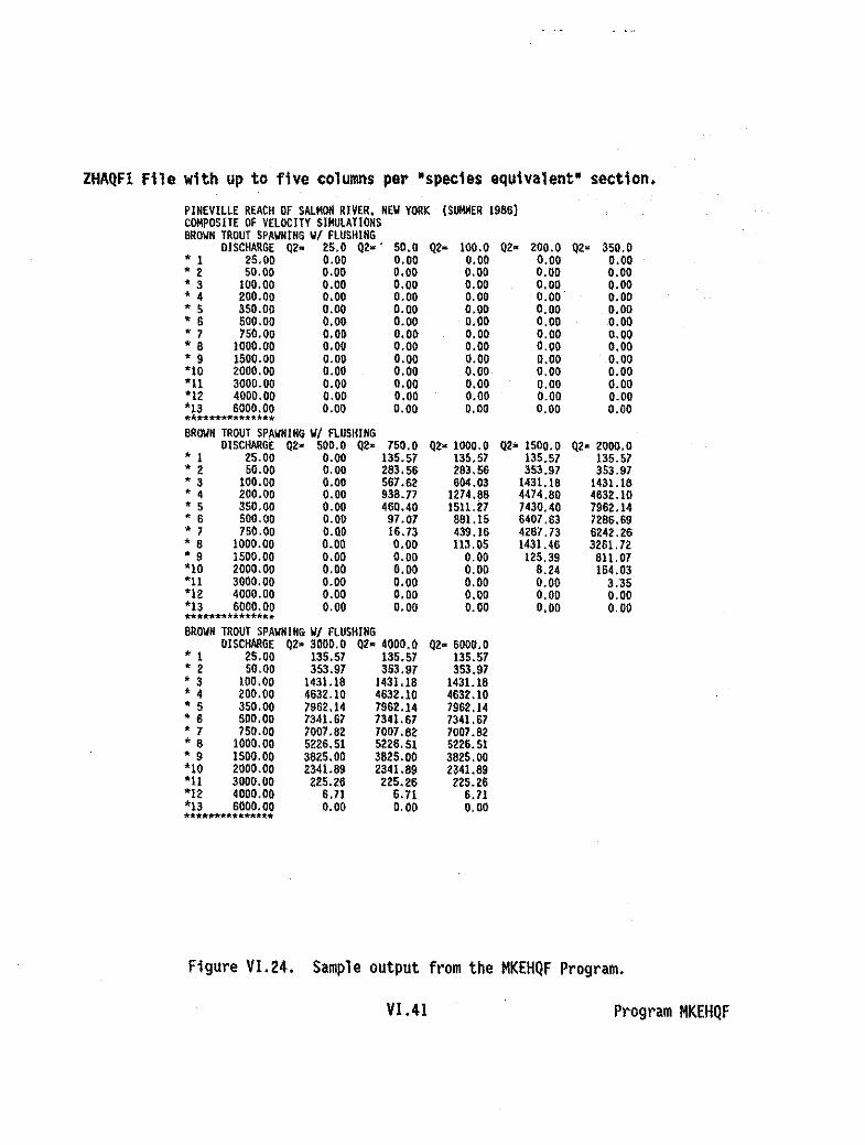
ZHAQFl File with up to five columns per ·species equivalent" section.
PINEVILLE REACH OF SALMON RIVER. NEW YORK (SUIIIIER 1986)COMPOSITE OF VELOCITY SIHULATIONSBROWN TROUT SPAWNING WI FLUSHING
DISCHARGE Q2- 25.0 Q2- 50.0 Q2- 100.0 Q2- 200.0 Q2' 350.0* 1 25,00 0,00 0,00 0,00 0.00 0.00* 2 50.00 0.00 0.00 0.00 0.00 0.00* 3 100,00 0.00 0.00 0.00 0.00 0.00* 4 200.00 0.00 0.00 0.00 0.00 0.00* 5 350.00 0,00 0.00 0.00 0.00 0.00* B 500.00 0.00 0.00 0.00 0.00 0.00* 7 750.00 0.00 0.00 0.00 0.00 0.00* 8 1000.00 0.00 0.00 0,00 0.00 0.00* 9 1500.00 0.00 0.00 0.00 0.00 0.00*10 2000.00 0.00 0.00 0.00 0.00 0.00*11 3000.00 0.00 0.00 0.00 0.00 0.00*12 4000.00 0.00 0.00 0,00 0.00 0.00*13 6000.00 0.00 0.00 0.00 0.00 0.00*,,"****"11*"'*"'.**BROWN TROUT SPAWNING WI Fl.USHING
DISCHARGE Q2- 500.0 Q2- 750.0* 1 25.00 0.00 135.57* 2 50.00 0.00 283,56* 3 100.00 0.00 567.62, 4 200.00 0.00 938.77* 5 350.00 0.00 460.40* 6 500.00 0.00 97.07* 7 750.00 0.00 16.73* 8 1000.00 0.00 0.00, 9 1500,00 0.00 0.00*10 2000.00 0.00 0.00"'11 3000.00 0.00 0.00'12 4000.00 0.00 0.00*13 6000.00 0.00 0.00*******:Il-******oItBROWN TROUT SPAWNING WI FLUSHING
DISCHARGE 02- 3000.0 Q2. 4000.0* 1 25.00 135.57 135.57, 2 50.00 353.97 353.97, 3 100.00 1431.18 1431.18, 4 200.00 4632.10 4632.10, 5 350.00 7962.14 1962.14* 6 500.00 7341.67 7341.67, 7 750.00 7007.82 1007.82* 8 1000.00 5226.51 5226.51* 9 1500.00 3825.00 3825.00*10 2000.00 2341.89 2341.89'II 3000.00 225.26 225.26*12 4000.00 6.71 6.71*13 6000,00 0.00 0.00**....n***Ir*****
Q2' 1000.0135.51283.56604.03
1274.881511. 27881.15439.16113.05
0.000.000.000.000.00
Q2- 6000.0135.57353.91
1431.184632.107962.147341.677007.B25226.513B25.002341.89225.28
6.710.00
02' 1500.0135.57353.97
1431.1B4474.807430.406407.634267.731431.46125.39
8.240.000.000.00
Q2- 2000.0135.57353.97
1431.184632.l07962.141286.696242.263261. 72811. 07164.03
3.350.000.00
Figure VI.24. Sample output from the MKEHQF Program.
VI.41 Program MKEHQF
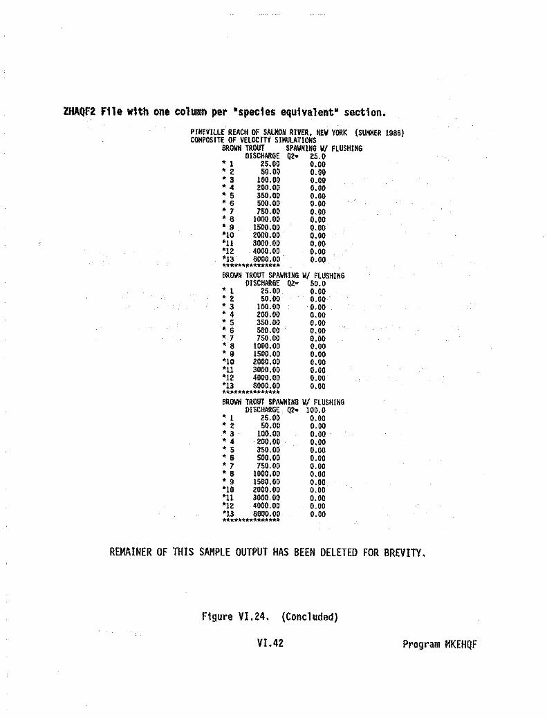
ZHAQF2 File with one column per 'species equivalent' section.
PINEVILLE' REACH OF SALMON RIVER, NE~ YORK (SUMMER 19SG)COHPOSITE OF VELOCITY SIMULATIONS
8R~ TROUT SPAWNING WI FLUSHINGDISCHARGE Q2- 25.0
* 1 25.00 0.00, 2 50.00 0.00• 3 100.00 0.00, 4 200.00 0.00, 5 350.00 0.00, 6 500.00 0.00, 7 750.00 0.00, 6 1000.00 0.00• 9 1500.00 0.00'10 2000.00 0.00'11 3000.00 0.00"12 4000.00 0.00"13 GOOO.OO ' 0.001\"****'lt.l1***'kfC'k**BROWN TROUT SPAWNING WI FLUSHING
OISCHARG£ Q2- 60.0* 1 25.00 0.00, 2 50.00 0.00, 3 100.00 0.00* 4 200.00 0.00* 5 350.00 0.00" G 500.00 0.00* 7 750.00 0.00"6 1000.00 0.00, 9 1500.00 0.00'10 2000.00 0.00"11 3000.00 0.00'12 4000.00 0.00'13 6000.00 0.00**-*'NW"''''***1i:ir**BROWN TROUT SPAWNING WI FLUSHING
OISCHARGE Q2- 100.0* 1 25.00 0.00, 2 50.00 0.00* 3 100.00 0.00, 4 200.00 0.00, 5 350.00 0.00, 6 500.00 0.00, 7 750.00 0.00" 8 1000.00 0.00" 9 1500.00 0.00"10 2000.00 0.00*11 3000.00 0.00"12 4000.00 0.00"13 6000.00 0.00**"'***'kl!:*******
REMAINER OF THIS SAMPLE OUTPUT HAS BEEN DELETED FOR BREVITY,
Figure VI.24. (Concluded)
VI.42 Program MKEHQF
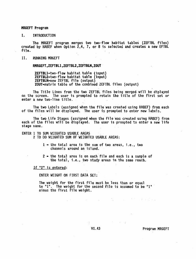
MRGEFT Program
I. INTRODUCTION
The MRGEFT program merges two two-flow habitat tables {ZEFTBL files}created by HABEF when Option 2,4, 7, or. B is selected and creates a new EFTBLfile.
II. RUNNING MRGEFT
RMRGEFT.ZEFT8Ll,ZEFTBL2,ZEFTBLN,ZOUT
ZEFTBll*two-flow habitat table {input}ZEFTBl2a two-flow habitat table (input)ZEFTBlH~new ZEFTBL file (output)ZOUTDmatrix table of the combined ZEFTBL files (output)
The Title Lines from the two ZEFTBL files being merged will be diplayedon the screen. The user is prompted to retain the title of the first set orenter a new two-line title.
The two Labels {assigned when the file was created using HABEF} from eachof the files will be displayed. The user is prompted to enter new labels.
The two Life Stages {assigned when the file was created using HABEF} fromeach of the files will be displayed. The user is'prompted to enter a new lifestage name.
ENTER 1 TO SUM WEIGHTED USABLE AREAS2 TO 00 WEIGHTED SUM OF WEIGHTED USABLE AREAS:
1 ~ the total area is the sum of two areas, i.e., twochannels around an island.
2 a the total area is on each file and each is a sample ofthe total, i.e .• two study ar~as in the same reach.
If "2" is entered:
ENTER WEIGHT ON FIRST DATA SET:
The weight for the first file must be less than or equalto "1". The weight for the second file is assumed to be "1 q .
minus the first file weight.
VI.43 Program MRGEFT
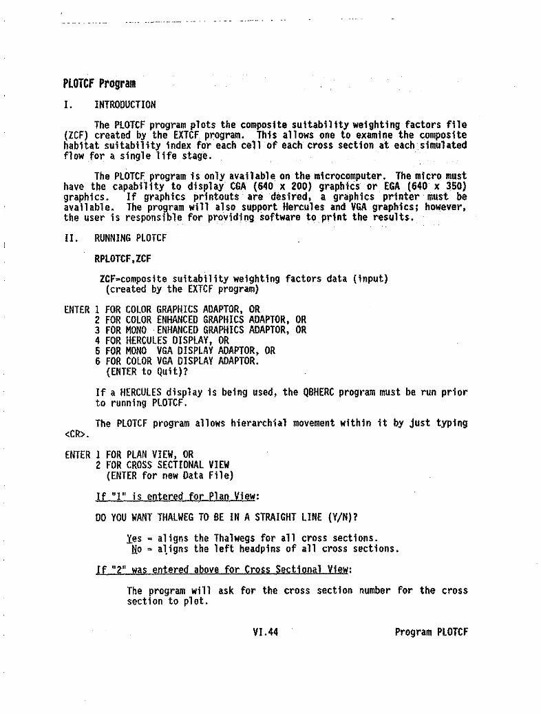
PlOTCF Progralll
I. INTRO~UCTION
The PLOTCF program plots the composite sUitability weighting factors file(ICF) created by the EXTCF program. This allows one to examine the compositehabitat sUitability index for each cell of each cross section at each simulatedflow for a single life stage.
The PLOTCF program is only available on the microcomputer. The micro llJusthave tile capability to display CGA (640 x 200) graphics or EGA (640 x 350)graphics. If graphics printouts are desired, a graphics printer must beavailable. The program will also support Hercules and VGA graphics; however,the user is responsible for providing software to print the results.
II. RUNNING PLOTCF
RPlOTCF,ICF
ZCFwcomposite suitability weighting factors data (input)(created by the EXTCF program)
ENTER 1 FOR COLOR GRAPHICS ADAPTOR, OR2 FOR COLOR ENHANCED GRAPHICS ADAPTOR, OR3 FOR MONO .ENHANCED GRAPHICS ADAPTOR, OR4 FOR HERCULES DISPLAY, OR5 FOR MONO VGA DISPLAY ADAPTOR, OR6 FOR COLOR VGA DISPLAY ADAPTOR.
(ENTER to Quit)?
If a HERCULES display is being used, the QBHERC program must be run priorto running PLOTCF.
The PLOTCF program allows hierarchial movement within it by just typing<CR>.
ENTER 1 FOR PLAN VIEW, OR2 FOR CROSS SECTIONAL VIEW
(ENTER for new Data File)
If "I" is entered for Plan View:
DO YOU WANT THALWEG TO BE IN A STRAIGHT LINE (YIN)?
yes. aligns the Thalwegs for all cross sections.No w a1igns the left headpins of all cross sections.
If "2" was entered above for Cross Sectional View:
The program will ask for the cross section number for tile crosssection to plot.
VI. 44 Program PlOTCF

In both cases, a list of flows will be displayed on the screen, and theuser will be asked to enter a flow number for the flow to plot.
NOTES:
1. The cross sectional view fails to shade cells that are not completelysubmerged at the chosen flow. These edge cells often are prime habitat.Comparing the cross sectional plot with the plan view will show omissions.
2. The plan view display fails to show the water's edge. Comparison of theplan view plot with the cross sectional plot will show the water's edge.
3. Distinction between shading types, and division boundaries between thecells themselves, is difficult if cells are quite narrow.
VI.45 Program PLOTCF

TRNHCF Program
I. INTRODUCTION
The TRNHCF program converts an unformatted ZHCF file to a formatted ZHCFfile, or it converts a formatted ZHCF file to an unformatted ZHCF file. A ZHCFfile is created by setting IOC(13)=1 in theHABTAT, HABTAV, orHABTAE programs.
Unformatted files are likely to be incompatible between a microcomputerand the CDC mainframe, and between different microcomputers. The formattedversion of the files should be used when transferring from computer to computer~
II. RUNNING TRNHCF
RTRHHCF,ZHCF,ZHCFN
ZHCF=unformatted or formatted file of cell areas and cell weightedusable areas (input) ... .
ZHCFN=new ZHCF file that is either formatted or unformatted.dependingon whether the input file was formatted or unformatted (output)
ENTER 1 FOR UNFORMATTED TO FORMATTED2 FOR FORMATTED TO UNFORMATTED
VI.46 Program TRNHCF

PROGRAM DESCRIPTION
Writes the data from a habitat versusstreamflow file into a format that maybe useful for report purposes.
VII. REPORT GENERATION PROGRAMS
INTRODUCTION
The standard output from the P~BSIH programs is not always in a formatmost useful for report purposes. The following programs have been developed toallow the user to format output to better meet his needs when writing reports.
PROGRAMS THAT REFORMAT AZHAQF FILE
PROGRAM BATCH/PROCEDURENAME fIL~NAHE FUNCTION
HABOUTA RHBOUTA ReportGeneration
HABOUTS
HABAE
RHBOUTS
RHABAE
ReportGeneration
ReportGeneration
VII.l
RHBOUTA,ZHAQF,ZOUT
ZHAQF~habitat vs. flow file (input)ZOUT-HABOUTA results (output)
Writes the data from a habitat versusstreamflow file into a format that may·be useful for report purposes, and sumsthe life stage values into one habitatversus streamflow figure for each lifestage for each flow. The ZHAQF filebeing used as input is assumed to havebeen generated using conditional covercurves as input to the habitatsimulation program.
RHBOUTS,ZHAQF,ZOUT
lHAQF=habitat vs. flow file (input)ZOUT-HABOUTS results (output)
Writes the data from a ZHAQF file intoa format that may be useful for reportpurposes, and calculates the minimumadult equivalent habitat area for eachlife stage for each flow.
RHABAE.ZHAQF •lOUT .ZHAQFN
ZHAQF-habitat vs. flow file (input)IOUT=HABAE results (output)ZHAQFN=new ZHAQF file with equivalenthabitat area (output)

PROGRAMS THAI REFORMAT A FISHCRY FILE
BATCH/PROCEDUREFILENAME FUNCTION
PROGRAMNAME
LSTCP RLSTCP ReportGeneration
PROGRAM DESCRIPTION
Reads a FISHCRV fil e and creates a fil e~ith one species set per page.
RLSTCP,FISHCRV,ZOUT
FlSHCRV-formalted curves file (input)ZOUT-lSTCP results (output)
PROGRAMS THAI REFORMAT AZEFTBL FILE
EFHTBL REFHTBL ReportGeneration
ZHCF FILE LISTING
Writes the data from a two-flow habitattable (ZEFTBl file), created byselecting Option 2, 4, 7, or 8 inHABEF, into a format that may be usefulfor report purposes.
REFHTBL,ZEFTBL,ZOUT
ZEFTBl-two-flow habitat table (input)ZOUT-EFHTBl results (output)
The following program lists information from the unformatted cell areasand cen weighted usable areas file (ZHCf) and may be useful for reportgeneration. Individual documentation for this program is located in ChapterVI.
lSTCEL RLSTCEL ZHCF Fileli sting
VII. 2
Lists the suitability of use factorsfor each cell in a pattern resemblinga map. This allows for the comparisonof factors in adjacent cells and howthe factors for a cell vary withdischarge. A"map· for each crosssection is generated.
RlSTCEL,ZHCF,TAPE3,ZOUT
ZHCF-unformatted cell areas and cellweighted usable areas (input)
TAPE3-unformatted cross section andreach data (input)
ZOUT-lSTCEl results (output)

PROGRAM DESCRIPTION
TAPES AND TAPE4 LISTING PROGRAMS
The following programs list information from the Cross Section andHydraul ic Properties files (TAPE3 and TAPE4) and may be useful for reportgeneration. Individual documentation for these programs is located in ChapterIll.
PROGRAM BATCH/PROCEDURENAME FILENAME FUNCTION
CHPWSL
LSTP34
lSTVD
RCMPWSL
RlSTP34
RLSTVD
TAPE4LIsting
TAPE3/4Listing
TAPE3/4Listing
VIL3
Compares the water surface elevationsin two TAPE4 files.
RCMPWSL,TAPE4A.TAPE4B,ZOUT,TAPE3
TAPE4A=TAPE4 file (input)TAPE4B=TAPE4 file (input)ZOUT=WSl comparison listing of thetwo TAPE4's (output)
TAPE3-title 1ines read from the TAPE3,if supplied. If not supplied, useris prompted to enter two title 1ines(input)
Li sts the contents of a TAPE3 and TAPE4file.
RLSTP34,ZOUT,TAPE3.TAPE4
ZOUT-LSTP34 results (output)TAPE3-unformatted cross section andreach data (input)
TAPE4=unformatted flow data (input)
Lists the velocities and depths of thecells, and cross section data that arefound on a TAPE3 ,and TAPE4.
RlSTVD.ZOUT,TAPE3.TAPE4
ZOUT-LSTVO results (output)TAPE3-unformatted cross section andreach data (input)
TAPE4-unformatted flow data (input)

TAm AND TAPE4 LISTING PROGRAMS (Continued!
PROGRAM BATCH/PROCEDURENAME fILENAME FUNCTION PROGRAM DESCRIPTION
LSTWLf RLSTWLF TAPE3/4 .•Hi sce11 aneous
VII.4
Lists water surface elevations on aTAPE4, and calculates and lists theFroude number and mean channelvelocities for each cross section andeach flow.
RLSTWLF,ZOUT,TAPE3,TAPE4
ZOUT~LSTWLF results (output)TAPE3~unformatted cross section and
reach data (input)TAPE4~unformatted flow data (input)

II. RUNNING EFHTBL
REFHTBL.ZEFTBl.ZOUT
ZEFTBL*two-flow habitat table (input)ZOUT=EFHTBL results (output)
Figure VII.l contains sample output from the EFHTBL program.
•
OATE - 8B/09/29.TIME - 08/38/51.
PROGRAM - EFHTBLPA8E - I
SPAWNINGFLOWS
PINEVILLE REACH OF SALHON RIVER. NEW YORK (SUMMER 1986)COMPOSITE OF VELOCITY SIHULATIONSBROWN TROUT SPAWNING W/ FLUSHING
INCUBATION FLOWS
25.0 50.0 100.0 200.0 350.0 SOO.O 750.0 1000.0 1500.0 2000.0 3000.0
1--------------------------------------------------------------------------------------------------1
25.0 I 0.0 0.0 0.0 0.0 0.0 0.0 135.6 135.6 135.6 135.6 135.6t
50.0 ! 0.0 0.0 0.0 0.0 0.0 0.0 263.6 283.6 354.0 354.0 354.01
100.0 I 0.0 0.0 0.0 0.0 0.0 0.0 567.6 604.0 1431.2 1431.2 1431.2I
200.0 I 0.0 0.0 0.0 0.0 0.0 0.0 938.8 1274.9 4474.8 4632.1 4632.1I
350.0 I 0.0 0.0 0.0 0.0 0.0 0.0 460.4 1511.3 7430.4 7962.1 7962.11
500.0 I 0.0 0.0 0.0 0.0 0.0 0.0 97.1 881.2 8407.8 7286.7 7341.7I
750.0 I 0.0 0.0 0.0 0.0 0.0 0.0 16.7 439.2 4287.7 6242.3 7007.8I
1000.0 I 0.0 0.0 0.0 0.0 0.0 0.0. 0.0 113.1 1431.5 3261.7 5226.5I
1500.0 ! 0.0 0.0 0.0 0.0 0.0 0.0 0.0 0.0 125.4 811.1 3825.01
2000.0 ! 0.0 0.0 0.0 0.0 0.0 0.0 0.0 0.0 8.2 184.0 2341.9I
3000.0 I 0.0 0.0 0.0 0.0 0.0 0.0 0.0 0.0 0.0 3.3 225.3
Figure VII.l Sample output from the EFHTBL program.
VII.5 Program EFHTBL

HABAE Program
I. INTRODUCTION
The HABAE program writes the data from a habitat versus streamflow (ZHAQF)file into a format that may be useful for report purposes, and .it calculates theminimum adult equivalent habitat area for each life stage for each flow.
II. RUNNING HABAE
RHABAE,ZHAQF,ZOUT,ZHAQFN
ZHAQF~habitat vs. flow file (input)ZOUT=HABAE results (output)ZHAQFN=new ZHAQF file with equivalent habitat area (output)
ENTER 1 TO CONVERT FROM ENGLISH TO METRIC, 2 FOR NO CONVERSION
Enter "In if you want the output printed in Metric units instead of English(meters versus feet).
ENTER 1 FOR WUA PRINTED XX.XX, 2 FOR WUA PRINTED XX
Weighted usable area (WUA) and flow (Q) can be printed in the output withor without a decimal point.
ENTER 1 FOR Q PRINTED XX.XX, 2 FOR QPRINTED XX
ENTER 1 FOR ABINDING EDGE, 2 FOR NO BINDING EDGE
The binding edge is on the top of the paper.
If "I" is entered for a Binding Edge:
. HOW MANY LINES FOR BINDING EDGE
At this point the user will be prompted to enter an Adult Equivalent Areafor each life stage for each species in the ZHAQF file.
If prompted to enter a weight for the Total Area, enter "I" as the TotalArea does not need a weight. Total Area is usually the first heading in a ZHAQFfile.
ENTER I TO PRINT UNITS BELOW TABLE, 2 FOR NO PRINT OF UNITS
If "I" is entered, the follOWing will be printed below each tabledepending on if the units are in English or Metric:
Q IN CUBIC FEET PER SECOND, WUA IN SQUARE FEET PER 1000 FEETQ IN CUBIC METERS PER SECOND, WUA IN SQUARE METERS PER 1000 METERS
Figure VII.2 contains sample output from the HABAE program.
VII.6 Program HABAE

Output contained in ZOUT file.
88/OS/27.07.50.57.
88/0B/Z7.07.50.57.
UPPER SALMON RIVER. MEAR STANLEY. IDAHOZHAQF FILE GENERATED BY HABTAT
Q VS. AVAILABLE HABITAT AREA PER 1000 FEET OF STREAM FOR TOTAL AREA
Q AREA EQUIVALENT
'B 227M 2278910 24395 2439520 29444 2944430 3174B 31HB40 33660 3366050 39436 3943560 42818 4281870 44512 4451Z80 458Z0 4582090 47187 47187
100 48495 48495UO 49535 49535IZO 50843 50B43130 51663 51883
WEIGHT ONLIFE STAGE 1.00
DISCHARGE 1M CU8lC FEET PER SECOND. WUA 1M SQUARE FEET PER 1000 FEET
UPPER SALMON RIVER. NEAR STANLEY. IDAHOZHAQF FILE GENERATED 8Y HABTAT
Q VS. AVAILABLE HABITAT AREA PER 1000 FEET OF STREAM FOR RAINBOW TROUT
Q FRY JUVENILE ADULT EQUIVALENT
8 594 0 80 010 3B6 0 10Z 020 257 0 IB5 030 75 208 260 28040 141 395 333 33350 419 495 432 432GO 211 492 547 54770 56 691 651 32980 59 690 740 29390 39 676 830 195
100 4 S96 912 19110 0 513 970 0120 0 621 1055 .0130 0 729 1114 0
WEIGHT ONLIFE STAGE 5.00 1.50 1.00
DISCHARGE IN CUBIC FEET PER SECOND. ··WUA IN SQUARE FEET PER 1000 FEET
Figure.VII.2 Sample output from the HABAE program.
VII.7
PROGRAM . HABAEPAGE I
PROGRAM • HADAEPAGE 2
Program HABAE

Output contained in ZHAQFH file.
UPPER SAU40N RIVER, HEAR STAHLEY. IDAHONEIl ZHAQF FILE GENERATED 5Y HA8AE
OiSCHARGE EQUIVAlENTI' s.OO ZZ788.90Z' 10.00 24395.063' ZO.OO 29444.044' 30.00 91747.525' 40.00 39659.656' 50.00 39436.347' 60.00 42818.31a' 70.00 44512.379' ao.Oo 458Z0.Z0
10' 90.00 47187.19II' 100.00 48494.81IZ' 110.00 49535.0419' IZO.OO 5084Z.6614' 130.00 51882.89*';*-*********'/11
DISCHARGE EQUIVALENT1* 8.002' 10.003' 20.004' 30.005* 40.00 '6' 50.007' 50.00S' 70.009' SO.OO
10' 90.00II' 100.0012' lIO.OO13' IZO.OO14' 130.00**********i;I;**1t
0.000.000.00
Z59.7333Z.98432.45547.08328.65Z93.35194.80
. 19.400.000.000.00
Figure VII.2 (Concluded)
VILa Program HABAE
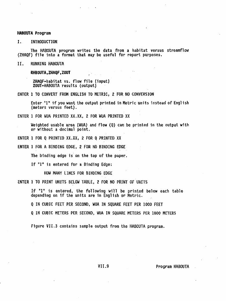
KARMA Program
I. INTRODUCTION
The HABOUTA program writes the data from a habitat versus streamflow(ZHAQF) file into a format that may be useful for report purposes.
II. RUNNING HABOUTA
RHBOUTA,ZHAQF,ZOUT
ZHAQF-habitat vs. flow file (input)ZOUT-HABOUTA results (output)
ENTER I TO CONVERT FROM ENGLISH TO METRIC, 2 FOR NO CONVERSION
Enter "I" if you want the output printed in Metric units instead of Engl ish(meters versus feet).
ENTER 1 FOR WUA PRINTED XX. XX, 2 FOR WUA PRINTED XX
Weighted usable area (WUA) and flow (Q) can be printed in the output withor without a decimal point.
ENTER 1 FOR Q PRINTED XX.XX, 2 FOR QPRINTED XX
ENTER 1 FOR A BINDING EDGE, 2 FOR NO BINDING EDGE
The binding edge is on the top of the paper.
If "1" is entered for a Binding Edge:
HOW MANY LINES FOR BINDING EDGE
ENTER 1 TO PRINT UNITS BELOW TABLE, 2 FOR NO PRINT OF UNITS
If "I" is entered, the following will be printed below each tabledepending on if the units are in English or Metric.
Q IN CUBIC FEET PER SECOND, WUA IN SQUARE FEET PER 1000 FEET
Q IN CUBIC METERS PER SECOND, WUA IN SQUARE METERS PER 1000 METERS
Figure VII.3 contains sample output from the HABOUTA program.
VII.9 Program HABOUTA

68/0a/Z7,07.41.ZZ.
UPPER SALMO!I RIVER. HEAR STAHLEY. IDAHOZHAQF FILE GENERATED BY HABTAT
Q VS. AVAILABLE HABITAT AREA PER 1000 FEET OF STREAM FOR TOtAL AREA
Q AREA
PROGRAlI • tlABOlITAPAGE 2
128456789
1011121314
B.OO10.0020.0080.0040.0050.0060.0070.00ao.oo90.00
100.00110.00120.00130.00
2278B.9024395.0629444.0481747.5233659.5639436.8442618.3144512.8745820.2047187.1948494.8149535.0450842.5851882.89
68/08/27.07.41.22.
Q IN CUBIC FEET PER SECOND. WUA IN SQUARE FEET PER 1000 FEET
UPPER SALMON RIVER. NEAR STANLEY, IDAHOZHAQF FILE GENERATED BY HABTAT
Q VS. AVAILABLE HABITAT AREA PER 1000 FEET OF StREAM FOIl RAINBOW TROUT
Q FRY JUVENILE ADULT
1 8.00 593.92 0.00 79.872 10.00 885.61 0.00 101.703 20.00 256.72 0.00 185.364 30.00 78.00 207.80 259.735 40.00 140.67 395.44 332.986 50.00 418.61 495.20 432.487 60.00 211.13 491.81 547.088' 70.00 85.73 891.28 860.56 .9 60.00 5B.87 869.96 740.38
10 90.00 38.95 575.61 630.3411 100.00 3.68 598.44 911.5912 110.00 0.00 512.90 970.4813 120.00 0.00 621.43 10$4.9014 130.00 0.00 726.64 1113.86
Q IN CUBIC FEET PER SECOND. WUA IN SQUARE FEET PER 1000 FEET
PRCGRAM - HAllOUTAPAGE 3
Figure VII.3 Sample output from the HABOUTA program.
VIr. 10 Program HABOUTA

MABOUTS Program
I. INTRODUCTION
The HABOUTS program writes the data from a habitat versus streamflow(ZHAQF) file into a format that may be useful for report purposes, .and it sumsthe life stage values into one habitat vs. flow figure for each life stage foreach flow. The ZHAQF file being used as input is assumed to have been generatedusing conditional cover curves as input to the habitat simulation program.
II. RUNNING HABOUTS
RHBOUTS.ZfV\QF.ZOUT
ZHAQF=habitat vs. flow file (input)ZOUT=HABOUTS results (output)
ENTER 1 TO CONVERT FROM ENGLISH TO METRIC, 2 FOR NO CONVERSION
Enter "I" if you want the output printed in Metric units instead of English(meters versus feet).
ENTER 1 FOR WUA PRINTED XX.XX, 2 FOR WUA PRINTED XX
Weighted usable area (WUA) and flow (Q) can be printed in the output withor without a decimal point.
ENTER·l FOR QPRINTED XX.XX, 2 FOR Q PRINTED XX·
ENTER I FOR A BINDING EDGE, 2 FOR NO BINDING EDGE
The binding edge is on the top of the paper.
If "I" is entered for a Binding Edge:
HOW MANY LINES FOR BINDING EDGE
ENTER I TO PRINT UNITS BELOW TABLE, 2 FOR NO PRINT OF UNITS
If "I" is entered, the following will .be printed below each tabledepending on if the units are in English or Metric:
Q IN CUBIC FEET PER SECOND, WUA IN SQUARE FEET PER 1000 FEET
Q IN CUBIC METERS PER SECOND, WUA IN SQUARE METERS PER 1000 METERS
Figure VII.4 contains sample output from the HABDUTS program. The ZHAQFfile used as input to the SUMHQF program (Figure V.27) was used as input to theHABOUTS program to generate these results.
VII.II Program HAROUTS

88/08/27.07.45.14.
88/0U27.07.45.14.
ALTMAR REACH OF SALMON RIVER. NEW yORKCOMPOSITE OF VELOCITIES AHO SECTIONS AS ISLANOS
Q VS. AVAILA8LE HA81TAT AREA PER 1000 FEET OF STREAM FOR TOTAL AREA
Q AREA SUM
1 25 155830 1558302 50 177487 1774873 100 196137 1961374 200 216445 216445S 350 255153 2551536 500 275933 2759337 750 290595 2905958 1000 299067 2990679 1500 314227 314227
10 2000 324867 32486711 3000 336215 33621512 4000 342061 34206113 6000 353206 353206
Q IN CU81C FEET PER SECOND. WUA IN SOUARE FEET PER 1000 fEET
ALTMAR REACH OF SALMON RIVER. NEW YORKCOMPOSITE OF VELOCITIES ANO SECTIONS AS ISLAN05
PROGRAM - HASOUTSPAGE I
PROGRAM - HA80UrSPAGE 2
QVS. AVAILA8LE HA81TAT AREA PER 1000 FEET OF STREAM FOR WINTER STEELHEAO . FRY
Q NO COV ONC SM 08J L6 08J COM80 SUM
1 25 36805 16307 0 21790 25244 1001452 50 42488 29453 78 27012 30050 1290803 100 49470 52287 497 36939 38997 1781904 200 57007 75435 1680 54869 55733 a447245 350 53624 72840 11397 72371 73695 2839276 500 57626 80677 13612 86037 85775 3237267 750 42776 76006 17617 97045 88449 3218928 1000 44224 66900 17214 99282 87951 3155719 1500 33173 51387 11575 93601 84917 274652
10 2000 30240 45082 9715 89564 78887 25348711 3000 41442 52684 8969 99457 85295 28784712 4000 40433 52567 9092 91380 74054 26752613 6000 38948 52588 9178 75138 53161 229013
Q IN CU81C FEET PER SECOND. WUA IN SQUARE FEET PER 1000 FEET
SAMPLE OUTPUT TERMINATED HERE FOR BREVITY.
Figure VII.4 Sample output from the HABOUTS program.
VII,12 Program HABOUTS

LSTCP Program
I. INTRODUCTION
The lSTCP program reads a FISHeRV file and writes a file with one speciesset per page. The species indicator is the first four numbers assigned as thecurve set ro number (family 'and species); the last two numbers, indicate lifestage. Therefore, all curve sets using the same first four numbers as a curveset 10 number will be listed on the same page.
II. RUNNING lSTCP
RlSTCP.FISHCRV.ZOUT
FISHCRV-formatted curves file (input)ZOUT-lSTCP results (output)
ENTER 1 FOR A BINDING EDGE, 2 FOR NO BINDING EDGE
The binding edge is on the top of the paper. '
If "I" is entered for a Binding Edge:
HOW MANY LINES FOR BINDING EDGE
DATE - 88/01fl8 T1KE - 22.31.4B. PAG£ - 1
RECREATION SUITABILITY 0' USE CRITERIA - SALKOR RIVER STunYH 720101 10 6 5 0 BOATING ' TU81N6V720101 0.00 0.52 1.00 1.00 2.00 1,00 4.00 1.00 5.00 1.00 6.00 0.80V720101 8.00 0.50 9.00 0.&0 10.00 0.00100.00 0.00o 710101 0.00 0.00 0,50 0.00 1.00 0.00 2.00 1.00 10.00 1.00100.00 1.00S 720101 0.00 1.00 5.00 1.00 10.00 1.00 15.00 1.00100.00 1.00H 720102 1011 5 0 BOATING CANOEINGV,720102 0.00 0.60 0.40 1.00 2.00 1.00 4.00 1,00 6.00 1.00 7.00 1.00V720102 8.00 0.80 9.00 0.52 10.00 0.00100.00 0.00o 720102 ~.50 1.00 3.00 1.00 4.00 1.00 10.00 1.00100.00 1.00'5720102 0.00 1.00 5.00 1.00 10,00 1.0015.00 1.00100.00 1.00
The following would appear on the second page.
DATE - 88/01/28 TIME - 22.31.48. PAGE· 2
RECREATION SUITABILITY OF USE CRITERIA' SALMON RIVER STUDYH 720201 9 9 5 0 WATER CONTACT SWIMMINGV720201 0.00 0.56 0.30 1.00 0.80 1.00 I.DO 0.94 2.00 0.50 3.00 0.00V720201 4.00 0.00 10.00 0.00100.00 0.000720201 0.00 0.00 1.00 0.00 2.00 0.00 2.50 0.00 3.00 0.50 3.50 0.800720201 4.00 1.00 10.00 1.00100.00 1.00S 720201 0.00 1.00 5.DO 1.00 10.00 1.00 15.00 1.00100.00 1.00
Figure VII.5. Sample output from the LSTCP program.
VII.l3 Program lSTCP

IFG incremental methodology20 minute slide-tape program
VIII. REFERENCES AND OTHER RELATED REPORTS
Anonymous. 1981. Instream flow field techniques manual. Cooperative InstreamFlow Group. Revised.
Bartholow, J.M. 1989. Stream temperature investigations: field and analyticmethods. Instream Flow Information Paper No. 13. U.S. Fish Wildl. ServoBiol. Rep. 89(17). 139 pp.
Bartholow, J.M., and T.J. Waddle. 1986. Introduction to stream network habitatanalysis. Instream Flow Information Paper No. 22. U.S. Fish Wildl. ServoBioI. Rep. 86(8). 242 pp.
Bovee, K.D. 1982. Aguide to stream habitat analysis using the Instream FlowIncremental Methodology. Instream Flow Information Paper No. 12. U.S. FishWildl. Servo FWS/OBS~82/26. 248 pp.
Bovee, K.D. 1986. Development and evaluation of habitat suitabil ity criteriafor use in the Instream Flow Incremental Methodology. Instream FlowInformation Paper No. 21. U.S. Fish Wild. Servo BioI. Rep. 86(7). 235 pp.
Control Data Corporation. NOS Reference Manual, Vol. 1. CDC Manual No. 60435400.
Control Data Corporation. NOS Reference Manual, Vol. 2. CDC Manual No. 60445300.
Control Data Corporation. NOS Time-sharing user's guide. CDC Manual No. 60436400.
Control Data Corporation. NOS Time-sharing user's reference. CDC ManualNo. 60435500.
Control Data Corporation. XEDIT Reference Manual. CDC Manual No. 60455730.
Cooperative Instream Flow Service Group. 1979.overview. U.S. Fish Wild. Servo WjIFG-80j31.on the incremental methodology.
Cooperative Instream Flow Service Group. 1980. IFG incremental methodology site selection. U.S. Fish Wildl. Servo W/IFG-83jW09. 1S minute slide-tapeprogram on the incremental methodology.
Crance, J.H., and J. Shoemaker. 1986. 18-minute slide-tape on development anduse of suitability index curves for Use in instream flow studies. U.S. FishWildl. Servo NEC-86/2I. 27 pp.
Milhous, R. T. 1978. A computer program for the determination of averagehydraulic and shape parameters of a stream cross section (IFGIA). U.S. FishWildl. Serv., National Ecology Research Center, Fort Collins, Colorado. 71pp.
VIlLI

Milhous, R.T. 1983. Instream flow values as a factor in water management.Pages 231-237 in R.J. Charbeneau and B.P. Popkin, eds. Regional and Statewater resources planning and management. American Water Resources Association,Bethesda, MO.
Milhous, R.T. 1986. Comparison of minimum instream flow needs. Pages 2089-2097in M. Karamouz, G.R. Baumli, and W.J. Brick, eds. Water from '86: worldwater issues in evolution. ASCE, New York.
Milhous, R.T. 1987. Discussion of hydraulics of high-gradient streams. Journalof Hydraulic Engineering, Vol. 113, No. 7,American Society of Civil Engineers,New York. pp. 921-923.
Milhous, R.T. [1989.] Hydraulics in the Physical Habitat Simulation System.Instream Flow Information Paper No. 19. In preparation.
Mi1hous, R.T., D.l. Wegner, and T. Waddle. 1981; User's guide to the PhysicalHabitat Simulation System (PHABSrM). Instream Flow Information Paper No. II.U.S. Fish Wild1. Servo FWS/GBS-Sl/43 (revised). 475.pp.
Nestler, J.M., J. Fritschen, R.T. MOhous, and J. Troxel. 1986. Effects (}fflow alterati(}ns on trout, angling, and recreation in the Chattahoochee Riverbetween Buford Dam and Peachtree Creek. Technical ReportE-86-IO, WaterExperiment Station, U.S. Army Corps of Engineers, Vicksburg, MS. 73 pp.
Nestler, J.M., R.T. Milhous, and J.B. Layzer. [1989.] Instream habitat modelingtechniques. In J. Gore, ed. Alternatives in regulated river management. CRCPublishing Co., Boca Raton, Florida. In preparation. .
Rantz, S.E., and others. 1982. Measurement and computation of streamflow. U.S.Geological Survey Water Supply Paper 2175. Washington, DC.
Stalnaker, C.B. 1980. The use of habitat structure proterenda for establishingflow regimes necessary for maintenance of fish habitat. Pages 321-337 in J.F.Ward and J.A. Stanford, eds. The ecology of regUlated streams. PlenumPublishing Corporation, New York, NY.
Theurer, F.T., K.A. Voos, and W.J. Miller. 1984. Instream water temperaturemodel. Instream Flow Information Paper No. 16. U.S. Fish Wildl. Serv.FWS/OBS-S4/15. 372 pp.
U.S. Armj Corps of Engineers. 1985. HEC-2 water surface profiles user's manual.Hydrologic Engineering Center, U.S. Army Corps of Engineers, 609 Second St.,Davis, California.
U.S. Bureau of Reclamation. 1968. Guide for application of the water surfaceprofile computer program. Hydrology Branch, Denver, CO~ 36 pp.
VIrI.2