physical review d 074016 (2005) pion-pion scattering amplitudejpac/scatteringref/2000s/pion-pion...
TRANSCRIPT

PHYSICAL REVIEW D 71, 074016 (2005)
Pion-pion scattering amplitude
J. R. PelaezDepartamento de Fısica Teorica, II (Metodos Matematicos), Facultad de Ciencias Fısicas, Universidad Complutense de Madrid,
E-28040, Madrid, Spain
F. J. YndurainDepartamento de Fısica Teorica, C-XI Universidad Autonoma de Madrid, Canto Blanco, E-28049, Madrid, Spain
(Received 3 December 2004; published 18 April 2005)
1550-7998=20
We obtain reliable �� scattering amplitudes consistent with experimental data, both at low and highenergies, and fulfilling appropriate analyticity properties. We do this by first fitting experimental lowenergy (s1=2 � 1:42 GeV) phase shifts and inelasticities with expressions that incorporate analyticity andunitarity. In particular, for the S wave with isospin 0, we discuss in detail several sets of experimental data.This provides low energy partial wave amplitudes that summarize the known experimental information.Then, we impose Regge behavior as follows from factorization and experimental data for the imaginaryparts of the scattering amplitudes at higher energy, and check fulfillment of dispersion relations up to0.925 GeV. This allows us to improve our fits. The ensuing �� scattering amplitudes are then shown toverify dispersion relations up to 1.42 GeV, as well as s� t� u crossing sum rules and other consistencyconditions. The improved parametrizations therefore provide a reliable representation of pion-pionamplitudes with which one can test chiral perturbation theory calculations, pionium decays, or use asinput for CP-violating K decays. In this respect, we find �a�0�0 � a�2�0 �2 � �0:077� 0:008�M�2
� and��0�0 �m2
K� � ��2�0 �m2K� � 52:9� 1:6o.
DOI: 10.1103/PhysRevD.71.074016 PACS numbers: 13.75.Lb, 11.55.Jy, 11.80.Et, 12.39.Fe
I. INTRODUCTION
A precise and unbiased knowledge of the �� scatteringamplitude has become increasingly important in recentyears. This is so, in particular, because �� scattering isone of the few places where one has more observables thanunknown constants in a chiral perturbation theory (ch.p.t.)analysis to one loop, so it provides a test of ch.p.t. in thisapproximation, as well as a window to higher order terms.Beside this, an accurate determination of the S wavescattering lengths, and of the phase shifts, providesessential information for three subjects under intensiveexperimental investigation at present, viz., light scalarspectroscopy, pionic atom decays, and CP violation inthe kaonic system.
In two recent papers, Ananthanarayan, Colangelo,Gasser, and Leutwyler [1] and Colangelo, Gasser, andLeutwyler [2] have used experimental information, analy-ticity and unitarity (in the form of the Roy equations [3])and, in the second paper, also chiral perturbation theory, toconstruct a precise �� scattering amplitude at low energy,s1=2 � 0:8 GeV. Unfortunately, however, the analysis ofRefs. [1,2] presents some weak points. First of all, the inputscattering amplitude at high energy (s1=2 * 1:5 GeV)which these authors use is incompatible with experimentaldata [4] on �� cross sections and also contradicts knownproperties of standard Regge theory; see a detailed analysisin Refs. [5–7] and Appendix B here. Moreover, the errorsthese authors take for some of their experimental input dataare optimistic, as shown in Ref. [7]. As a consequence ofall this the �� amplitudes of Ref. [2] do not satisfy well a
05=71(7)=074016(31)$23.00 074016
number of consistency tests, as we show in Sec. VII here(see also Refs. [6,7] for more details).
Some of the shortcomings of the articles in Refs. [1,2],notably incorrect Regge behavior, are also reproducedin the papers of Descotes et al., and Kaminski, Lesniak,and Loiseau [8], who also base their analysis in theRoy equations but, since the errors given by these authorsare substantially larger than those of Ref. [2], theireffects are now less pronounced. Therefore, we stillneed to find reliable pion-pion scattering amplitudes com-patible with physical data both at high and low energy, aswell as to verify to what extent such amplitudes agreewith ch.p.t.
In the present paper we address ourselves to the firstquestion; that is to say, we try to find what experimentimplies for the �� amplitudes. To avoid biases, we willstart by performing fits to experimental data on phase shiftsand inelasticities, incorporating only the highly safe re-quirements of analyticity and unitarity, in the low energyregion s1=2 � 1:42 GeV. In particular, for the S0 wavebelow 0.95 GeV, where the experimental situation is con-fused, we perform a global fit, as well as individual fits tovarious sets of data. These fits are described in Sec. II and,in the following sections, we investigate to which extentthe ensuing scattering amplitudes are consistent, in par-ticular, with high energy information. To do so, we assumeRegge behavior, as given in Ref. [5] (slightly improved; seeAppendix B), above 1.42 GeV: using this we check inSec. III fulfillment of forward dispersion relations, forthe three independent �� scattering amplitudes. This, inparticular, permits us to discriminate among the various
-1 2005 The American Physical Society
J. R. PELAEZ AND F. J. YNDURAIN PHYSICAL REVIEW D 71, 074016 (2005)
sets of phase shifts for the S0 wave, leaving only a fewsolutions which are consistent with dispersion relations(and, as it turns out, very similar one to the other, asdiscussed in Sec. IV).
When dealing with different data sets one has to weighnot only the data on a single experiment but one has to takeinto account the reliability of the experiments themselves.So we have done for many waves, where some clearlyfaulty experimental data have only been considered toconservatively enlarge the uncertainties. Concerning themost controversial S0 wave, we have used the very reliabledata coming from Kl4 and K ! �� decays; to this we addthe results from other experimental analyses of �� scat-tering available in the literature, either separately or com-bined in a global fit. We then use forward dispersionrelations to test consistency of the several sets of data.
The present study should therefore be considered, inparticular, as a guideline to the consistency (especiallywith forward dispersion relations) of the various data sets.
Next, we use these dispersion relations to improve thecentral values of the parameters of the fits given in Sec. II.The result of such analysis (Sec. IV) is that one can get aprecise description for all waves, consistent with forwarddispersion relations up to s1=2 0:95 GeV and a bit less so( & 1:5� level) in the whole energy range, 2M� � s1=2 �1:42 GeV, and even below threshold, down to s1=2 ����2
pM�. The greater uncertainties affect the S0 wave for
s1=2 > 0:95 GeV, a not unexpected feature, and, to a lesserextent, the P wave above 1:15 GeV.
In Sec. V we verify that the scattering amplitudes wehave obtained, which were shown to satisfy s� u crossing(by checking the dispersion relations), also verify s� tcrossing, in that they satisfy two typical crossing sum rules.In Sec. VI we use the scattering amplitudes we havedetermined and the method of the Froissart-Gribov repre-sentation to calculate a number of low energy parametersfor P, D and some higher waves which, in particular,provides further consistency tests. We also evaluate, inSec. VII, the important quantities �a�0�0 � a�2�0 �2 and��0�0 �m2
K� � ��2�0 �m2
K� for which we find
�a�0�0 � a�2�0 �2 � �0:077� 0:008�M�2� ;
��0�0 �m2
K� � ��2�0 �m2K� � 52:9� 1:6o:
Also in Sec. VII we compare our results with those ob-tained by other authors using Roy equations and ch.p.t.However, in the present paper we will not address our-selves to the question of the chiral perturbation theoryanalysis of our �� amplitudes.
Our paper is finished in Sec. VIII with a brief summary,as well as with a few appendixes. In Appendix A, wecollect the formulas obtained with our best fits. InAppendix B we give a brief discussion of the Regge for-mulas used; in particular, we present an improved evalu-ation of the parameters for rho exchange. Appendix C is
074016
devoted to a discussion of the shortcomings of experimen-tal phase shift analyses above 1:4 GeV, which justifiesour preference for using Regge formulas in this energyregion.
We end this introduction with a few words on notationand normalization conventions. We will here denote am-plitudes with a fixed value of isospin, say I, in channel s,simply byF�I�, f�I�l ; we will specify the channel, F�Is�, whenthere is danger of confusion. For amplitudes with fixedisospin in channel t, we write explicitly F�It�.
For scattering amplitudes with well-defined isospin inchannel s, Is, we write
F�Is��s; t� � 2�X
l�even
�2l 1�Pl�cos��f�Is�l �s�; Is � even;
F�Is��s; t� � 2�Xl�odd
�2l 1�Pl�cos��f�Is�l �s�; Is� odd;
f�I�l �s� �2s1=2
�kf�I�l ; f�I�l � sin��I�l �s�ei�
�I�l �s�: (1.1a)
The last formula is only valid when only the elastic channelis open. When inelastic channels open this equation is nomore valid, but one can still write
f l�s� ���le
2i�l � 1
2i
�: (1.1b)
The factor 2 in the first formulas in (1.1a) is due to Bosestatistics. Because of this, even waves only exist withisospin I � 0; 2 and odd waves must necessarily haveisospin I � 1. For this reason, we will often omit theisospin index for odd waves, writing e.g. f1, f3 insteadof f�1�1 , f�1�3 . Another convenient simplification that we usehere is to denote the�� partial waves by S0, S2, P, D0, D2,F, etc., in self-explanatory notation.
The quantity �l, called the inelasticity parameter forwave l, is positive and smaller than or equal to unity. Theelastic and inelastic cross sections, for a given wave, aregiven in terms of �l and �l by
�ell �
1
2
�1 �2
l
2� � cos2�l
�; �inel
l �1� �2
l
4;
(1.2)
�ell ; �
inell are defined so that, for collision of particles A, B
(assumed distinguishable),
�tot �4�2
�1=2�s;mA;mB�
2s1=2
�k
Xl
�2l 1���ell �inel
l �:
(1.3)
When neglecting isospin violations (which we dounless explicitly stated otherwise) we will take the con-vention of approximating the pion mass by M� � m�� ’
139:57 MeV. We also define scattering lengths, a�I�l , and
-2

sw
s00 0
FIG. 1. The mapping s! w.
PION-PION SCATTERING AMPLITUDE PHYSICAL REVIEW D 71, 074016 (2005)
effective range parameters, b�I�l , by
�
4M�k2l Refl�s� ’k!0
a�I�l b�I�l k2 � � � ;
k ����������������������s=4�M2
�
q:
(1.4)
II. THE �� SCATTERING AMPLITUDES AT LOWENERGY (s1=2� 1:42 GeV)
We present in this section parametrizations of the S, P,D, F, and G waves in �� scattering obtained fitting ex-perimental data at low energy, s1=2 � 1:42 GeV, whichwill provide a representation of the experimental �� scat-tering amplitudes in this energy range: this may be con-sidered as an energy-dependent phase shift analysis. Above1:42 GeV, we will use the Regge expressions obtained inRef. [5], which we reproduce and discuss in Appendix B inthe present paper. In following sections we will verify towhich extent the scattering amplitudes that one finds in thisway are consistent with dispersion relations or crossingsymmetry, within the errors given.
Before entering into the actual fits, a few words are dueon the choice of the energy 1:42 GeV as limit between theregions where we use phase shift analyses and Reggerepresentations. Experimental phase shift analyses existup to 2 GeV. However, as is known, phase shift analysesbecome ambiguous as soon as inelastic processes becomeimportant. As we will discuss in some detail inAppendix C, the existing experimental phase shift analysesbecome suspect for energies above 1:4 GeV: in particu-lar, they produce cross sections that deviate from experi-mentally measured total cross sections.
As for the higher energy range, we have shown inRef. [5] that a Regge description of the imaginary part ofthe �� scattering amplitudes agrees well with �� crosssection data (and, through factorization, also with �N andNN data) for kinetic energies above 1 GeV; for ��scattering, down to s1=2 ’ 1:4, or even to 1:3 GeV, depend-ing on the process. We have chosen the limiting energy tobe 1:42 GeV as a reasonable compromise; but one couldhave taken lower limits, or slightly higher ones, as well. Infact, it is not possible to go below 1:4 GeV with a Reggedescription for the It � 1 amplitude or for�0�0 scattering,since both contain the isospin zero amplitudes, which showtwo resonances just below that region [the f2�1270� and thef0�1370�]. But it is possible to choose a lower junctionpoint between the phase shift analyses and the Reggeformulas for �0� scattering. The influence of this isnegligible for �0� , as we will show in Sec. III A 2,provided one stays in the range 1:32 GeV � s1=2 �1:42 GeV, with the larger values favored.
We now turn to the parametrizations. In writing them wewill use the requirements of analyticity and elastic unitar-ity. Extra information has been added to help stabilize thefits in those channels where the low energy data are scarce;
074016
in particular, information on Adler zeros or scatteringlengths. For the latter we impose values obtained fromtheir Froissart-Gribov representation, but with enlargederror bars.
The method used to take into account unitarity andanalyticity will be the standard one of the effective rangeformalism, supplemented by a conformal expansion. To beprecise, for a given partial wave f�I�l �s� we write, for anyvalue (complex or real) of s,
f�I�l �s� �2s1=2
�k1
2s1=2k�2l�1��I�l �s� � i
�k2l
�1
��I�l �s� � ik2l 1=2s1=2
: (2.1)
The effective range function ��I�l �s� is real on the segment
0 � s � s0, but it will be complex above s0, and also fors � 0. Here s0 is the energy squared above which inelasticprocesses are nonnegligible. Using only the requirementsof causality and conservation of probability, it can beshown that ��I�
l �s� is analytic in the complex s plane, cutfrom �1 to 0 and from s0 to 1; see Fig. 1.
We can profit from these analytical properties as follows.We map the cut plane into the unit disk (as in Fig. 1) bymeans of the conformal transformation
w�s� �
���s
p�
�������������s0 � s
p
���s
p
�������������s0 � s
p :
The properties of analyticity and elastic unitarity of f�I�l �s�are then strictly equivalent to uniform convergence (in thevariable w) in the disk jwj< 1 of the series
��I�l �s� �
X1n�0
Bnw�s�n:
This series thus converges, in the variable s, uniformly inthe interior of the whole cut plane; in general very quickly.It will turn out that we will need only two or three terms inthe expansions for the partial wave amplitudes.
-3

0 002 004 006 008 0001 0021 0041s
2/1 )VeM(
0
05
001
051
002δ1 )s(
.tif oN .rotcaf mrof morF
.la te ucsepopotorP
nitraM & skoorbatsE
.la te smayH
)2 tes( ucsepopotorP
)tif ygrene hgih( YP
FIG. 2 (color online). The phase shifts of solution 1 fromProtopopescu et al. [10], Hyams et al. [11(a)], and Estabrooksand Martin [11(a)] compared with the prediction with theparameters (2.6) (solid line below 1 GeV). We emphasize thatthis is not a fit to these experimental data, but is obtained fromthe pion form factor [9]. The error here is like the thickness ofthe line. Above 1 GeV, the dotted line and error (PY) are asfollows from the fit (2.7).
J. R. PELAEZ AND F. J. YNDURAIN PHYSICAL REVIEW D 71, 074016 (2005)
Before starting with the actual fits, we here say a fewwords on the values of s0 (i.e., the energy at which weconsider inelasticity not negligible) that we will take forthe various waves. For the S0 wave, the �KK channel isstrongly coupled, so here s0 � 4m2
K. For other waves the�KK channel is weakly coupled. In the cases where we have
sufficiently precise data (that is, for the P wave and the lowenergy S2 wave), we will take s1=20 � 1:05 GeV which is,approximately, the 2�" threshold.
For the D0 wave, and for the S2 wave at intermediateenergy, 1:05 GeV & s1=2 & 1:4 GeV, inelasticity is de-tected. It is small (but not negligible) while, unfortunately,the data are not precise enough to perform a fully consis-tent analysis. We then follow a different strategy: we fit theexperimental phase shifts using formulas that neglect in-elasticity below 1:45 GeV (which is, approximately, the 2"threshold). The experimental inelasticity between 1 and1:42 GeV is then added by hand.
Finally, for the D2, F waves, for which experimentsdetect no inelasticity below 1:42 GeV, s0 is taken equalto 1:45 GeV.
A. The P wave
1. Parametrization of the P wave below 1 GeV
We will consider first the P wave for �� scatteringbelow 1 GeV, to exemplify the methods, because it is theone for which more precise results are obtained. We startthus considering the region of energies where the inelas-ticity is below the 2% level; say, s1=20 � 1:05 GeV2.
We then expand �1�s� in powers of w, and, reexpressingw in terms of s, the expansion will be convergent over allthe cut s plane. Actually, and because we know that the Pwave resonates at s � M2
", it is more convenient to expandnot �1�s� itself, but �s� given by
�1�s� � �s�M2"� �s�=4; (2.2a)
so we write
�s� � fB0 B1w � � �g: (2.2b)
In terms of �1�s� we thus find the expression for thecotangent of the phase shift, keeping two terms in theexpansion,
cot�1�s� �s1=2
2k3�M2
" � s��B0 B1
���s
p�
�������������s0 � s
p
���s
p
�������������s0 � s
p
�;
s1=20 � 1:05 GeV: (2.3)
M";B0; B1 are free parameters to be fitted to experiment. In
074016
terms of �1; we have, for the rho width, and the scatter-ing length, a1,
�" �2k3"
M2" �M
2"�; k" �
1
2
������������������������M2" � 4M2
�
q;
a1 ��1
4M��1�4M2��
�1
M��M2" � 4M2
�� �4M2��:
(2.4)
The values B0 � const, Bi�1 � 0 would correspond to aperfect Breit-Wigner. Actually, it is known that the "deviates from a pure Breit-Wigner and for a precisionparametrization two terms, B0 and B1, have to be kept in(2.3). Note that the parametrization holds not only on thephysical region 4M2
� � s � s0, but on the unphysical re-gion 0 � s � 4M2
� and also over the whole region of thecomplex s plane with s � 0. The parametrization givennow is the one that has less biases, in the sense that nomodel has been used: we have imposed only the highly saferequirements of analyticity and unitarity, which followfrom causality and conservation of probability.
The best values for our parameters are actually obtainednot from fits to �� scattering data, but from fits to the pionform factor [9]. This is obtained from e� scattering, frome e� ! � �� and from $! %�� decay, where we havea large number of precise data, and pions are on their massshells. Including systematic experimental errors in the fits,and including in the fit also the constraint a1 � �38� 3� �10�3M�3
� for the scattering length, we have
-4

PION-PION SCATTERING AMPLITUDE PHYSICAL REVIEW D 71, 074016 (2005)
from � ��: B0 � 1:074� 0:006; B1 � 0:13� 0:04; M" � 774:0� 0:4 MeV
from � �0: B0 � 1:064� 0:006; B1 � 0:13� 0:04; M" � 773:1� 0:6 MeV:(2.5a)
The fit is excellent; one has &2=d:o:f: � 245=�244� 13�, and the slight excess over unity is due to the well-knownincompatibility of OPAL and other data for $ decay at low invariant mass.
The corresponding values for the rho width, and P wave scattering length and effective range parameter, are
a1 � �37:8� 0:8� � 10�3M�3� ; b1 � �4:74� 0:09� � 10�3M�5
� ; �"0 � 146:0� 0:8; from � ��
a1 � �37:8� 0:8� � 10�3M�3� ; b1 � �4:78� 0:09� � 10�3M�5
� ; �" � 147:7� 0:7; from � �0:(2.5b)
400 600 800 1000 1200 1400s
1/2 (MeV)
-30
-25
-20
-15
-10
-5
0 δ0
(2)(s)
PY improved
PY from data
CGL
Cohen et al.
Losty et al.
Hoogland et al. A
Hoogland et al. B
Durusoy et al. (OPE)
Durusoy et al.(OPE+DP)
FIG. 3 (color online). Continuous line: The I � 2, S-wavephase shifts, and error bands, corresponding to (2.7), (2.8a),(2.8b), and (2.9), denoted by PY. Dotted line: the fit fromRef. [6]. The experimental points are from Losty et al. (blacksquares), Hoogland et al. [12] solution A (black dots), and Cohenet al. [4] (black triangles). We have also included data fromDurusoy et al. and from solution B of Hoogland et al., althoughthey were not used in the fits. The dashed line, which lies belowour fit, is the S2 phase of Colangelo, Gasser, and Leutwyler [2]with error band attached.
Although the values of the experimental �� phase shiftswere not included in the fit, the phase shifts that (2.5a)implies are in very good agreement with them, as shown inFig. 2.
If neglecting violations of isospin invariance, one wouldexpect numbers equal to the average of both sets of pa-rameters in (2.5a). If we also increase the error, so as totake into account that due to isospin breaking, by addinglinearly half the difference between both determinations(2.5a), we find
B0 � 1:069� 0:011; B1 � 0:13� 0:05;
M" � 773:6� 0:9; a1 � �37:6� 1:1� � 10�3M�3� ;
b1 � �4:73� 0:26� � 10�3M�5� ; (2.6)
the corresponding parametrization we take to be valid up tos1=2 � 1 GeV.
2. The P wave for 1 GeV� s1=2� 1:42 GeV
In the range 1 GeV � s1=2 � 1:42 GeV one is suffi-ciently far away from thresholds to neglect their influence(the coupling to �KK is negligible). A purely empiricalparametrization that agrees with the data in Protopopescuet al. [10] and Hyams et al. [11(a)] up to 1.42 GeV, withinerrors, is obtained with a linear fit to the phase and in-elasticity:
�1�s� � �0 �1��������s=s
p� 1�; �1�s� � 1� '�
�������s=s
p� 1�;
' � 0:30� 0:15; �0 � 2:69� 0:01; �1 � 1:1� 0:2:
(2.7)
Here s � 1 GeV2. The value of �0 ensures the agreementof the phase with the value given in the previous subsectionat s � s � 1 GeV2. This fit is good (Fig. 2).
It should be remarked, however, that there are othersolutions for the P wave above 1:15 GeV. In the firstanalysis of Hyams et al. [11(a)], that we have followedhere, a resonance occurs with a mass 1:6 GeV, and itseffect is only felt above 1:4 GeV; but in the secondanalysis by the same group, Hyams et al. [11(b)] a broad,highly inelastic resonance (actually, more a spike than aresonance) with a mass 1:35 GeV appears, or does not
074016
appear, depending on the solution chosen. Finally, theParticle Data Group (based mostly on evidence frome e� annihilation and $ decay) report a resonance at1:45 GeV: one has to admit that the situation for the Pwave above 1:15 GeV is not clear. We will return to thislater.
B. The S waves
1. Parametrization of the S wave for I� 2
We consider three sets of experimental data. The firstcorresponds to solution A in the paper by Hoogland et al.[12], who use the reaction � p! � � n. We will notconsider the so-called solution B in this paper; while itproduces results similar to the other, its errors are clearlyunderestimated. The second set corresponds to the work ofLosty et al., [12] who analyze instead ��p! �����.
-5
J. R. PELAEZ AND F. J. YNDURAIN PHYSICAL REVIEW D 71, 074016 (2005)
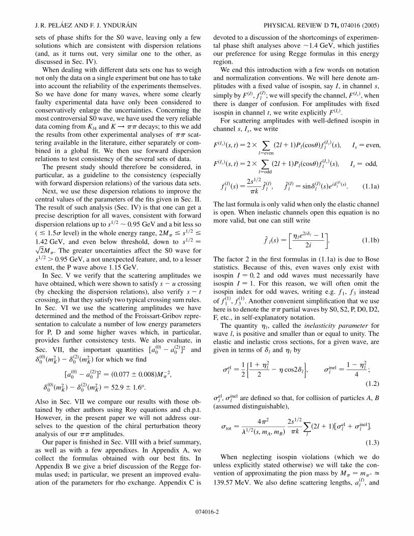
The third set are the data of Cohen et al. [4], who consider��n! ����p. These three sets represent a substantialimprovement over other determinations; since they pro-duce two like charge pions, only isospin 2 contributes, andone gets rid of the large S0 wave contamination. However,they still present the problem that one does not havescattering of real pions.
For isospin 2, there is no low energy resonance, butf�2�0 �s� presents the feature that a zero is expected (and,indeed, confirmed by the fits) in the region 0< s < 4M2
�.This zero of f�2�0 �s� is related to the so-called Adler zerosand, to lowest order in chiral perturbation theory, occurs ats � 2z22 with z2 � M�. We note that, unlike the corre-sponding zero for the S0 wave, 2z22 is inside the regionwhere the conformal expansion is expected to converge.
In Ref. [6], we neglected inelasticity below 1:45, andfitted all experimental data, for s1=2 � 1380 MeV. A moreprecise determination (and, above all, with more realisticerror estimates) is obtained if we realize that inelasticity isdetected experimentally above the 2�" threshold, s1=2 �1:05 GeV, so we should fit separately the low and highenergy regions (Fig. 3).
In the low energy region, we fix z2 � M� and fit only thelow energy data, s1=2 < 1:0 GeV; later, in Sec. IV, we willallow z2 to vary. We write
cot��2�0 �s� �s1=2
2kM2�
s� 2z22
�B0 B1
���s
p�
�����������s� s
p
���s
p
�����������s� s
p
�;
z2 � M�; s1=2 � 1:05 GeV: (2.8a)
074016
Then we get &2=d:o:f: � 13:0=�25� 2� and
B0 � �80:4� 2:8; B1 � �73:6� 12:6;
a�2�0 � ��0:052� 0:012�M�1� ;
b�2�0 � ��0:085� 0:011�M�3� :
(2.8b)
For the high energy region we neglect the inelasticitybelow 1:45 GeV , and then add inelasticity by hand. Weconsider two extreme possibilities: fitting the whole range,or fitting only high energy data (s1=2 � 0:91 GeV), requir-ing agreement of the central value with the low energydetermination at s1=2 � 1 GeV. We accept as the bestresult an average of the two, and thus have
cot��2�0 �s� �s1=2
2kM2�
s� 2M2�
�B0 B1
���s
p�
�������������s0 � s
p
���s
p
�������������s0 � s
p
�;
s1=20 � 1:45 GeV; B0 � �123� 6; B1 � �118� 14;
(2.9)
and we have enlarged the errors to cover both extremecases. We will not consider varying the position of theAdler zero for this high energy piece.
The inelasticity may be described by the empirical fit
��2�0 �s� �
�1� '�1� s=s�3=2; ' � 0:18� 0:12; s > s � �1:05 GeV�2;1; s < s � �1:05 GeV�2:
(2.10)
These formulas are expected to hold from s1=2 � 1:0 GeVup to 1:42 GeV. As shown in Fig. 3, both determinations,(2.8a), (2.8b), and (2.9) and that in Ref. [6] are almostoverlapping (their error bands actually overlap).
2. Parametrization of the S wave for I� 0 below0:95 GeV (global fit)
The S wave with isospin zero is difficult to deal with.Here we have a very broad enhancement, variously de-noted as '; �; f0, around s1=2 � +0 800 MeV. We willnot discuss here whether this enhancement is a bona fideresonance; we merely remark that in all experimentalphase shift analyses ��0�0 �s� crosses 90� somewhere be-tween 600 and 900 MeV; we define +0 as the energy atwhich the phase equals 90�. Moreover, we expect a zero off�0�0 �s� (Adler zero), hence a pole of the effective rangefunction ��0�
0 �s�, for s � 12 z
20 with 1
2 z20 in the region
0< s < 4M2�. Chiral perturbation theory suggests that
z0 ’ M�.
We can distinguish two energy regions: below s1=20 �
2mK we are under the �KK threshold. Between s1=20 ands1=2 1:2 there is a non-negligible coupling between the�KK and �� channels and the analysis becomes very
unstable, because there is little information on the process��! �KK and even less on �KK ! �KK. We will presentlater an empirical fit in the region of energies around andabove 1 GeV, and we will now concentrate in the lowenergy region.
For the theoretical formulas we impose the Adler zero ats � 1
2M2� (no attempt is made to vary this for the moment;
see Sec. IV), and a zero of cot��0�0 �s� at s � +20, +0 a free
parameter. Then we map the s plane, cut along the left handcut (s � 0) and the �KK cut, writing
cot��0�0 �s� �
s1=2
2kM2�
s� 12 z
20
+20 � s
+20
fB0 B1w�s� � � �g;
and
-6

FIG. 4 (color online). The I � 0, S-wave phase shifts and errorbands corresponding to Eq. (2.14a) and (2.14b) (PY, continuousline). Also shown (black dots) are the points from Kl4 and K2�decays, and only the high energy data included in the fits, asgiven in Eqs. (2.13a)–(2.13c). The dashed line is the solution ofColangelo et al. [2] .
PION-PION SCATTERING AMPLITUDE PHYSICAL REVIEW D 71, 074016 (2005)
w�s� �
���s
p�
�������������s0 � s
p
���s
p
�������������s0 � s
p ; s0 � 4m2K
(we have taken mK � 0:496 GeV).This parametrization does not represent fully the cou-
pling of the �KK channel and we will thus only take it to bevalid up to s1=2 � 0:95 GeV.
On the experimental side the situation is still a bitconfused, although it has cleared up substantially in recentyears thanks to the experimental information on Kl4 andK2� decays. The information we have on this S0 wave is ofthree kinds: from phase shift analysis in collisions[10,11(a)] �p! ��N;�; from the decay [13] Kl4; andfrom K2� decays. The last gives the value of the combina-tion ��0�
0 � ��2�0 at s1=2 � mK; the decay Kl4 gives ��0�0 � �1
at low energies, s1=2 & 380 MeV. If using recent K2�information [14] combined with older determinations,and with the I � 2 phase obtained in the previous subsec-tion, one finds the phase
��0�0 �m2K� � 43:3� 3�: (2.11)
We will here include in the fit the low energy data fromKl4 decay1 shown in Fig. 4, and we impose the value of��0�0 �m2
K� fromK2� given in (2.11). The main virtue of theseK decay data is that they refer to pions on their mass shell;but, unfortunately, this leaves too much room at the upperenergy range, s1=2 * 0:6 GeV. If we fit only K decay datawe can only use one-parameter B0 in the conformal ex-pansion: if including another parameter, spurious minimawould appear. We get a good fit, albeit with rather largeerrors:
cot��0�0 �s� �s1=2
2kM2�
s� 12 z
20
+20 � s
+20
B0; z0 � M�;
B0 � 18:5� 1:7; +0 � 766� 95 MeV;
&2
d:o:f:�
5:712� 2
: a�0�0 � �0:22� 0:02� �M�1� ;
��0�0 �mK� � 43� 5�:
(2.12)
To improve on this we have to add further data (and onemore parameter B1). To do so, we can follow two differentprocedures. We can add to the Ke4, K2� data various sets ofexperimental phase shifts, fitting each set individually; thiswe will do in Sec. III. Or we can follow what we considerto be the best procedure: we combine in the fit data from
1As a technical point, we mention that we have increased by50% the error in the point at highest energy, s1=2 � 381:4 MeV,from the Ke4 compilation of Pislak et al., because this experi-mental value represents an average over a long energy range thatextends to the edge of phase space.
074016
various experiments at energies above 0.8 GeV, which wewill call a global fit. The reason to choose only data above0.8 GeV is that, in the region between 0:81 GeV and0:97 GeV, the more relevant experimental results haveoverlapping error bars, something that does not happen atother energies (see Fig. 5). By combining several sets wemay expect to average out systematic errors, at least tosome extent.
At high energy we thus include the following sets ofdata: first of all, the values
��0�0 �0:8702 GeV2� � 91� 9�;
��0�0 �0:9102 GeV2� � 99� 6�;
��0�0 �0:9352 GeV2� � 109� 8�;
��0�0 �0:9652 GeV2� � 134� 14�:
(2.13a)
These points are taken from solution 1 of Protopopescu etal. [10] (both with and without modified moments), withthe error increased by the difference between this andsolution 3 data in the same reference. We will also includein the fit the data, at similar energies, of Grayer et al.[11(a)]
��0�0 �0:9122 GeV2� � 103� 8�;
��0�0 �0:9292 GeV�� � 112:5� 13�;
��0�0 �0:9522 GeV2� � 126� 16�;
��0�0 �0:9702 GeV2� � 141� 18�:
(2.13b)
The central values are obtained averaging the solutions
-7

FIG. 5 (color online). The I � 0, S-wave phase shifts and error band in the whole energy range as given by our fits (PY),Eqs. (2.14a), (2.14b), (2.15a), (2.15b), and (2.15b0). The experimental points from Kl4 and K2� decays are not shown.
J. R. PELAEZ AND F. J. YNDURAIN PHYSICAL REVIEW D 71, 074016 (2005)
given by Grayer et al., except2 solution E, and the error iscalculated adding quadratically the statistical error of thehighest point, the statistical error of the lowest point (foreach energy) and the difference between the central valueand the farthest point.
Finally, we add three points between 0.8 and 0.9 GeVobtained averaging the s-channel solution of Estabrooksand Martin and solution 1 of Protopopescu et al., whichrepresent two extremes. The error is obtained adding thedifference between these two in quadrature to the largeststatistical error. In this way we obtain the numbers,
��0�0 �0:8102 GeV2� � 88� 6�;
��0�0 �0:8302 GeV2� � 92� 7�;
��0�0 �0:8502 GeV2� � 94� 6�:
(2.13c)
In spite of the generous errors taken, it should be notedthat these data could still contain systematic errors, beyondthose taken into account in (2.13a)–(2.13c), which maycontaminate the results of the fit at the higher energies. InSec. IV we will use dispersion relations to improve theparametrization of this S0 wave.
2Solution E is incompatible with all other data sets in theregion above 0:8 GeV; we will discuss this in more detailbelow.
074016
We now have enough constraints to include two parame-ters Bi in the expansion of cot��0�
0 . We find
cot��0�0 �s� �
s1=2
2kM2�
s� 12 z
20
+20 � s
+20
�B0 B1
���s
p�
�������������s0 � s
p
���s
p
�������������s0 � s
p
�;
z0 �M�; B0 � 21:04; B1 � 6:62;
+0 � 782� 24 MeV; &2=d:o:f:� 15:7=�19� 3�:
a�0�0 � �0:230� 0:010�M�1� ;
b�0�0 � �0:268� 0:011�M�3� ;
��0�0 �mK� � 41:0� � 2:1�; (2.14a)
this fit (shown in Fig. 4) we take to be valid for s1=2 �0:95 GeV. The errors of the Bi are strongly correlated;uncorrelated errors are obtained if replacing the Bi by theparameters x; y with
B0 � y� x; B1 � 6:62� 2:59x;
y � 21:04� 0:70; x � 0� 2:6:(2.14b)
3. Parametrization of the S wave for I� 0 below0:95 GeV (individual fits)
In this subsection we summarize, in Table I, the resultsof fits to data from Kl4 and K2� decays including also,individually, data from various sets of phase shift analyses.
-8
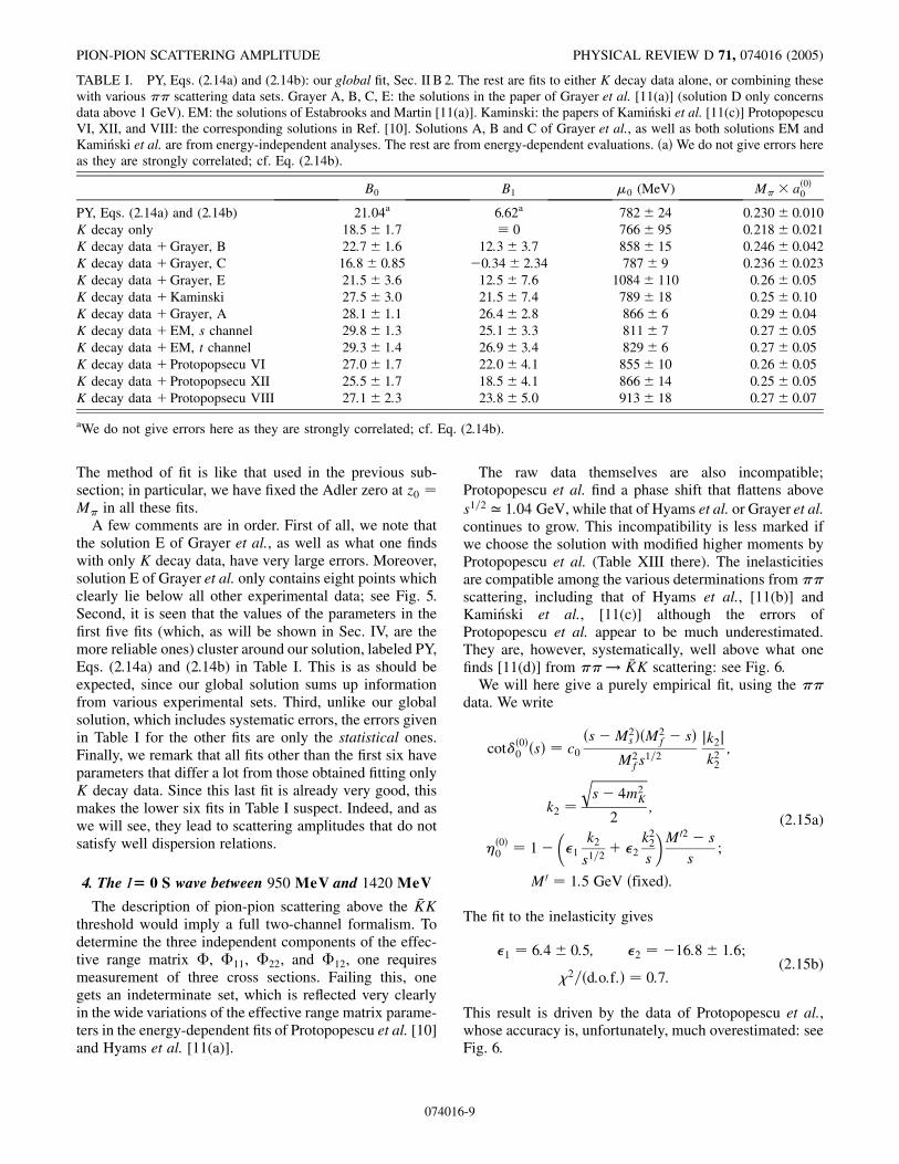
TABLE I. PY, Eqs. (2.14a) and (2.14b): our global fit, Sec. II B 2. The rest are fits to either K decay data alone, or combining thesewith various �� scattering data sets. Grayer A, B, C, E: the solutions in the paper of Grayer et al. [11(a)] (solution D only concernsdata above 1 GeV). EM: the solutions of Estabrooks and Martin [11(a)]. Kaminski: the papers of Kaminski et al. [11(c)] ProtopopescuVI, XII, and VIII: the corresponding solutions in Ref. [10]. Solutions A, B and C of Grayer et al., as well as both solutions EM andKaminski et al. are from energy-independent analyses. The rest are from energy-dependent evaluations. �a� We do not give errors hereas they are strongly correlated; cf. Eq. (2.14b).
B0 B1 +0 (MeV) M� � a�0�0
PY, Eqs. (2.14a) and (2.14b) 21:04a 6.62a 782� 24 0:230� 0:010K decay only 18:5� 1:7 � 0 766� 95 0:218� 0:021K decay data Grayer, B 22:7� 1:6 12:3� 3:7 858� 15 0:246� 0:042K decay data Grayer, C 16:8� 0:85 �0:34� 2:34 787� 9 0:236� 0:023K decay data Grayer, E 21:5� 3:6 12:5� 7:6 1084� 110 0:26� 0:05K decay data Kaminski 27:5� 3:0 21:5� 7:4 789� 18 0:25� 0:10K decay data Grayer, A 28:1� 1:1 26:4� 2:8 866� 6 0:29� 0:04K decay data EM, s channel 29:8� 1:3 25:1� 3:3 811� 7 0:27� 0:05K decay data EM, t channel 29:3� 1:4 26:9� 3:4 829� 6 0:27� 0:05K decay data Protopopsecu VI 27:0� 1:7 22:0� 4:1 855� 10 0:26� 0:05K decay data Protopopsecu XII 25:5� 1:7 18:5� 4:1 866� 14 0:25� 0:05K decay data Protopopsecu VIII 27:1� 2:3 23:8� 5:0 913� 18 0:27� 0:07
aWe do not give errors here as they are strongly correlated; cf. Eq. (2.14b).
PION-PION SCATTERING AMPLITUDE PHYSICAL REVIEW D 71, 074016 (2005)
The method of fit is like that used in the previous sub-section; in particular, we have fixed the Adler zero at z0 �M� in all these fits.
A few comments are in order. First of all, we note thatthe solution E of Grayer et al., as well as what one findswith only K decay data, have very large errors. Moreover,solution E of Grayer et al. only contains eight points whichclearly lie below all other experimental data; see Fig. 5.Second, it is seen that the values of the parameters in thefirst five fits (which, as will be shown in Sec. IV, are themore reliable ones) cluster around our solution, labeled PY,Eqs. (2.14a) and (2.14b) in Table I. This is as should beexpected, since our global solution sums up informationfrom various experimental sets. Third, unlike our globalsolution, which includes systematic errors, the errors givenin Table I for the other fits are only the statistical ones.Finally, we remark that all fits other than the first six haveparameters that differ a lot from those obtained fitting onlyK decay data. Since this last fit is already very good, thismakes the lower six fits in Table I suspect. Indeed, and aswe will see, they lead to scattering amplitudes that do notsatisfy well dispersion relations.
4. The I� 0 S wave between 950 MeV and 1420 MeV
The description of pion-pion scattering above the �KKthreshold would imply a full two-channel formalism. Todetermine the three independent components of the effec-tive range matrix �, �11, �22, and �12, one requiresmeasurement of three cross sections. Failing this, onegets an indeterminate set, which is reflected very clearlyin the wide variations of the effective range matrix parame-ters in the energy-dependent fits of Protopopescu et al. [10]and Hyams et al. [11(a)].
074016
The raw data themselves are also incompatible;Protopopescu et al. find a phase shift that flattens aboves1=2 ’ 1:04 GeV, while that of Hyams et al. or Grayer et al.continues to grow. This incompatibility is less marked ifwe choose the solution with modified higher moments byProtopopescu et al. (Table XIII there). The inelasticitiesare compatible among the various determinations from ��scattering, including that of Hyams et al., [11(b)] andKaminski et al., [11(c)] although the errors ofProtopopescu et al. appear to be much underestimated.They are, however, systematically, well above what onefinds [11(d)] from ��! �KK scattering: see Fig. 6.
We will here give a purely empirical fit, using the ��data. We write
cot��0�0 �s� � c0
�s�M2s ��M
2f � s�
M2fs
1=2
jk2j
k22;
k2 �
������������������s� 4m2
K
q2
;
��0�0 � 1�
'1
k2s1=2
'2k22s
M02 � s
s;
M0 � 1:5 GeV �fixed�:
(2.15a)
The fit to the inelasticity gives
'1 � 6:4� 0:5; '2 � �16:8� 1:6;
&2=�d:o:f:� � 0:7:(2.15b)
This result is driven by the data of Protopopescu et al.,whose accuracy is, unfortunately, much overestimated: seeFig. 6.
-9

FIG. 6 (color online). Fit to the I � 0, S-wave inelasticity andphase shift between 950 and 1400 MeV. Data from Refs. [10,11].The difference between the determinations of ��0�
0 from ��!
�� (PY from data) and from ��! �KK (PY alternative) isapparent here.
J. R. PELAEZ AND F. J. YNDURAIN PHYSICAL REVIEW D 71, 074016 (2005)
If, instead of fitting ��0�0 to the �� data of Protopopescu
et al. and Hyams et al. we had fitted the data [11(d)] from��! �KK scattering (shown in Fig. 6), we would havefound values for the 'i much smaller than what was givenin (2.15b):
'1 � 2:4� 0:2; '2 � �5:5� 0:8; &2=�d:o:f:� � 1:3:
(2.15b0)
We have checked that the influence of using (2.15b) or(2.15b0) on the dispersion relations and other evaluations ofintegrals, to be considered later, is minute, for energiesbelow 0:95 GeV. This is because the inelasticity affectslittle the imaginary part of the partial wave (on the aver-age). Above 1 GeV, if we took the 'i following from��! K �K, Eq. (2.15b0), the dispersion relations wouldbe slightly better fulfilled; see Sec. IVA, at the end. Inspite of this, we stick to (2.15b). Taking ��0�
0 from one set ofexperiments and ��0�0 from another (incompatible with thefirst) would be an inconsistent procedure.
To fit ��0�0 we also require it to agree with the low energydetermination we found in Sec. II B 2 at s1=2 � 0:95 GeV.If we include the data of Protopopescu et al. in the fit wefind a poor fit with &2=d:o:f: � 39=�14� 2� and the pa-rameters
c0 � 1:72� 0:08; Ms � 920 MeV;
Mf � 1340 MeV:
The error in c0, corresponding to 3�, is purely nominal. Ifwe keep Ms fixed and remove the data of Protopopescuet al., we get a good &2=d:o:f:, and now
074016
c0 � 0:79� 0:25; Mf � 1270 MeV:
If we want to be compatible with the data of Hyams et al.,we must increase the errors. We then take the numbers
c0 � 1:3� 0:5; Mf � 1320� 50 MeV;
Ms � 920 MeV �fixed�:(2.16)
The fit is shown in Fig. 6.We emphasize again that these are purely empirical fits
and, moreover, they are fits to data which certainly haveuncertainties well beyond their nominal errors, as given ingiven in (2.15b) and (2.16); something that is obvious for��0�
0 from Fig. 6. It follows that relations such as dispersionrelations in which the S0 wave plays an important role willbe unreliable for energies near and, especially, above �KKthreshold (below these energies, however, both (2.15b) and(2.15b0) give very similar results). In fact, we will checkthat mismatches occur when s1=2 > 0:95 GeV. A sounddescription of the S0 wave for s1=2 > 0:95 GeV in ��scattering would require more refined parametrizationsand, above all, use of more information than just ��experimental data, and lies beyond the scope of the presentpaper.
C. The D waves
The D waves cannot be described with the same accu-racy as the S, P waves. The data are scanty, and have hugeerrors. That one can get reasonable fits at all is due to thefact that one can use low energy information from sumrules; specifically, we will impose in the fits the values ofthe scattering lengths that follow from the Froissart-Gribovrepresentation. Note that this is not circular reasoning, andit only introduces a small correlation: the Froissart-Gribovrepresentation for the D0, D2, F waves depends mostly onthe S0, S2 and P waves, and very little on the D0, D2, Fwaves themselves.
1. Parametrization of the I� 2 D wave
For isospin equal 2 we would only expect importantinelasticity when the channel ��! "" opens up, so wewill take the value s0 � 1:452 GeV2 4M2
" for the energyat which elasticity is not negligible.
But life is complicated: a pole term is necessary to get anacceptable fit down to low energy since we expect ��2�
2 tochange sign near threshold. The experimental measure-ments (Losty et al.; Hoogland et al. [12]) give negativeand small values for the phase above some 500 MeV, whilechiral perturbation calculations and the Froissart-Gribovrepresentation indicate a positive scattering length [6]. Ifwe want a parametrization that applies down to threshold,we must incorporate this zero of the phase shift. What ismore, the clear inflection seen in data around 1 GeV im-plies that we will have to go to third order in the conformalexpansion. So we write
-10

004 006 008 0001 0021 0041s
2/1)VeM(
7-
6-
5-
4-
3-
2-
1-
0
δ2)2(
)s(
.la te ytsoL
.la te dnalgooH
.la te nehoC
atad morf YP
devorpmi YP
LGCA
)EPO( .la te yosuruD
)PD-EPO( la te yosuruD
FIG. 7 (color online). Fits to the I � 2, D-wave phase shift.Continuous line (PY) with Eq. (2.18). Dashed line: PY, afterimproving with dispersion relations (Sec. IV). Dotted line: the fitused in Refs. [1,2] (ACGL, CGL). Also shown are the data pointsof Losty et al., from solution A of Hoogland et al. [12], fromCohen et al. [4], and Durusoy et al. [12], the last not included inthe fit.
3For these data we arbitrarily take a common error of 10%.
PION-PION SCATTERING AMPLITUDE PHYSICAL REVIEW D 71, 074016 (2005)
cot��2�2 �s� �s1=2
2k5fB0 B1w�s� B2w�s�2g
�M�
4s
4�M�2 �2� � s
(2.17a)
with � a free parameter fixing the zero and
w�s� �
���s
p�
�������������s0 � s
p
���s
p
�������������s0 � s
p ; s1=20 � 1450 MeV:
Since the data we have on this wave are not accurate (cf.Fig. 7) we have to include extra information. To be precise,we include in the fit the value of the scattering length thatfollows from the Froissart-Gribov representation,
a�2�2 � �2:78� 0:37� � 10�4M�5� ;
but not that of the effective range parameter,
b�2�2 � ��3:89� 0:28� � 10�4M�7�
(see below, Sec. VI).We get a mediocre fit, &2=d:o:f: � 71=�25� 3�, and the
values of the parameters are
B0 � �2:4� 0:3� � 103; B1 � �7:8� 0:8� � 103;
B2 � �23:7� 3:8� � 103; � � 196� 20 MeV:
(2.17b)
We have rescaled the errors by the square root of the&2=d:o:f:
The fit, which may be found in Fig. 7, returns reasonablenumbers for the scattering length and for the effective
074016
range parameter, b�2�2 :
a�2�2 � �2:5� 0:9� � 10�4M�5� ;
b�2�2 � ��2:7� 0:8� � 10�4M�7� :
(2.18)
Although the twist of ��2�2 �s� at s1=2 1:05 GeV isprobably connected to the opening of the 2�" channel,we neglect the inelasticity of the D2 wave, since it is notdetected experimentally. This, together with the incompati-bility of the various sets of experimental data and the poorconvergence of the conformal series, indicates that thesolution given by (2.17a) and (2.17b) is, very likely, some-what displaced with respect to the ‘‘true’’ D2 wave at thehigher energy range (say for s1=2 * 0:7 GeV). In fact, thevalues of the parameters will be improved in Sec. IV withthe help of dispersion relations; the D2 phase shift onefinds by so doing is slightly displaced with respect to thatfollowing from (2.17a) and (2.17b), as shown in Fig. 7.
2. Parametrization of the I� 0 D wave
The D wave with isospin 0 in�� scattering presents tworesonances below 1:7 GeV: the f2�1270� and the f2�1525�,that we will denote, respectively, by f2, f02. Experi-mentally, �f2 � 185� 4 GeV and �f02 � 76� 10 GeV:The first, f2, couples mostly to ��, with small couplingsto �KK (4:6� 0:5%), 4� (10� 3%), and ��. The secondcouples mostly to �KK, with a small coupling to�� and 2�,respectively, 10� 3% and 0:8� 0:2%. This means that thechannels �� and �KK are essentially decoupled and, to a15% accuracy, we may neglect inelasticity up to s ’1:452 GeV2.
There are not many experimental data on the D wavewhich, at accessible energies, is small. So, the compilationof ��0�2 phase shifts of Protopopescu et al. [10] givessignificant numbers for ��0�
2 only in the range 810 MeV �
s1=2 � 1150 MeV. In view of this, it is impossible to getaccurately the D-wave scattering lengths, or indeed anyother low energy parameter, from this information: so, wewill include information on a�0�2 to help stabilize the fits.
We take the data of Protopopescu et al. [10] and considerthe so-called ‘‘solution 1,’’ with the two possibilities givenin their Tables VI and XIII (with modified higher mo-ments), in the range mentioned before, s1=2 � 0:810 GeVto 1:150 GeV. The problem with these data points is thatthey are certainly biased, as indeed they are quite incom-patible with those of other experiments. We can stabilizethe fits by fitting also the points3 of Estabrooks and Martin,[11(a)] and imposing the value of the width of the f2resonance, with the condition �f2 � 185� 10 MeV, aswell as the value of the scattering length. We write
-11
J. R. PELAEZ AND F. J. YNDURAIN PHYSICAL REVIEW D 71, 074016 (2005)
cot��0�2 �s� �s1=2
2k5�M2
f2� s�M2
�fB0 B1w�s�g (2.19a)
and
w�s� �
���s
p�
�������������s0 � s
p
���s
p
�������������s0 � s
p ; s1=20 � 1450 MeV;
Mf2 � 1275:4 MeV:
We find
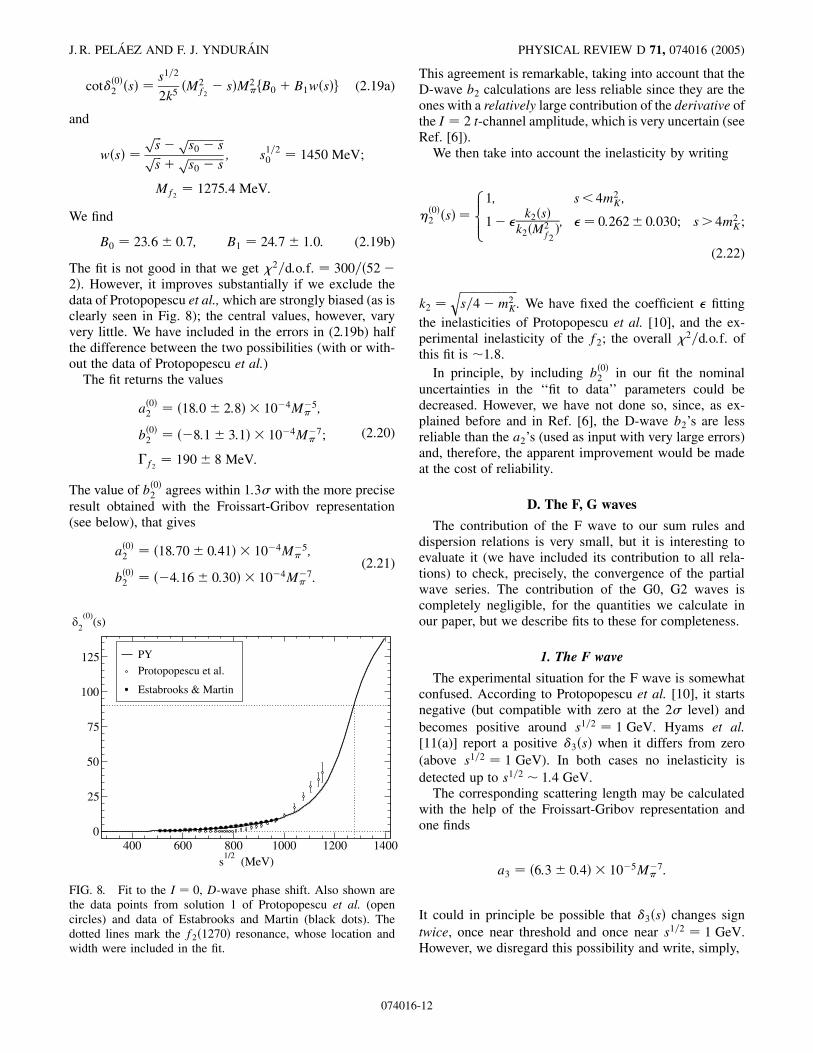
B0 � 23:6� 0:7; B1 � 24:7� 1:0: (2.19b)
The fit is not good in that we get &2=d:o:f: � 300=�52�2�. However, it improves substantially if we exclude thedata of Protopopescu et al., which are strongly biased (as isclearly seen in Fig. 8); the central values, however, varyvery little. We have included in the errors in (2.19b) halfthe difference between the two possibilities (with or with-out the data of Protopopescu et al.)
The fit returns the values
a�0�2 � �18:0� 2:8� � 10�4M�5� ;
b�0�2 � ��8:1� 3:1� � 10�4M�7� ;
�f2 � 190� 8 MeV:
(2.20)
The value of b�0�2 agrees within 1:3� with the more preciseresult obtained with the Froissart-Gribov representation(see below), that gives
a�0�2 � �18:70� 0:41� � 10�4M�5� ;
b�0�2 � ��4:16� 0:30� � 10�4M�7� :
(2.21)
400 600 800 1000 1200 1400s
1/2 (MeV)
0
25
50
75
100
125
δ2(0)
(s)
PY
Protopopescu et al.
Estabrooks & Martin
FIG. 8. Fit to the I � 0, D-wave phase shift. Also shown arethe data points from solution 1 of Protopopescu et al. (opencircles) and data of Estabrooks and Martin (black dots). Thedotted lines mark the f2�1270� resonance, whose location andwidth were included in the fit.
074016
This agreement is remarkable, taking into account that theD-wave b2 calculations are less reliable since they are theones with a relatively large contribution of the derivative ofthe I � 2 t-channel amplitude, which is very uncertain (seeRef. [6]).
We then take into account the inelasticity by writing
��0�2 �s� �
8><>:1; s< 4m2
K;
1� 'k2�s�k2�M
2f2�; '� 0:262� 0:030; s> 4m2
K;
(2.22)
k2 ����������������������s=4�m2
K
q: We have fixed the coefficient ' fitting
the inelasticities of Protopopescu et al. [10], and the ex-perimental inelasticity of the f2; the overall &2=d:o:f: ofthis fit is 1:8.
In principle, by including b�0�2 in our fit the nominaluncertainties in the ‘‘fit to data’’ parameters could bedecreased. However, we have not done so, since, as ex-plained before and in Ref. [6], the D-wave b2’s are lessreliable than the a2’s (used as input with very large errors)and, therefore, the apparent improvement would be madeat the cost of reliability.
D. The F, G waves
The contribution of the F wave to our sum rules anddispersion relations is very small, but it is interesting toevaluate it (we have included its contribution to all rela-tions) to check, precisely, the convergence of the partialwave series. The contribution of the G0, G2 waves iscompletely negligible, for the quantities we calculate inour paper, but we describe fits to these for completeness.
1. The F wave
The experimental situation for the F wave is somewhatconfused. According to Protopopescu et al. [10], it startsnegative (but compatible with zero at the 2� level) andbecomes positive around s1=2 � 1 GeV. Hyams et al.[11(a)] report a positive �3�s� when it differs from zero(above s1=2 � 1 GeV). In both cases no inelasticity isdetected up to s1=2 1:4 GeV.
The corresponding scattering length may be calculatedwith the help of the Froissart-Gribov representation andone finds
a3 � �6:3� 0:4� � 10�5M�7� :
It could in principle be possible that �3�s� changes signtwice, once near threshold and once near s1=2 � 1 GeV.However, we disregard this possibility and write, simply,
-12

PION-PION SCATTERING AMPLITUDE PHYSICAL REVIEW D 71, 074016 (2005)
cot�3�s� �s1=2M6
�
2k7fB0 B1w�s�g;
w�s� �
���s
p�
�������������s0 � s
p
���s
p
�������������s0 � s
p ;(2.23a)
with s1=20 � 1:45 GeV, and impose the value of a3.It is to be understood that this parametrization provides
only an empirical representation of the available data, andthat it may not be reliable except at very low energies,where it is dominated by the scattering length, and fors1=2 * 1 GeV. We fit data of Protopopescu et al. [10] forenergies above 1 GeV, and data of Hyams et al. [11(b)] Wehave estimated the errors of this last set (not given in thepaper) as the distance from the average value to the ex-treme values in the different solutions given. We find
&2
d:o:f:’
7:714� 2
; B0 � �1:09� 0:03� � 105;
B1 � �1:41� 0:04� � 105: (2.23b)
The errors have been increased by including as an error thevariation that affects the central values when using onlyone of the two sets of data. We do not include separatelythe effects of the "3�1690�, since its tail is incorporated inthe fitted data.
2. The G waves
The experimental information on the G waves is veryscarce. For the wave G2, we have two nonzero values for��2�4 from Cohen et al. [4] and four significant ones from
Losty et al. [12]; they are somewhat incompatible. We thenfit the data separately, with a one-parameter formula; wewrite
cot��2�4 �s� �
s1=2M8�
2k9B:
If we fit the data of Losty et al. we find B � ��0:56�0:09� � 106, while from Cohen et al. we get B ���10:2� 3:0� � 106. Fitting both sets together we findB � �9:1� 106, and a very poor &2=d:o:f: � 32=�6�1�. Enlarging the resulting error to cover 6�, we obtainour best result,
cot��2�4 �s� �s1=2M8
�
2k9B; B � ��9:1� 3:3� � 106:
(2.24)
This formula can only be considered as valid only for alimited range, 0:8 � s1=2 � 1:5 GeV. In fact, from theFroissart-Gribov representation it follows that the G2 scat-tering length is positive. One has a�2�4 � �4:5� 0:2� �10�6M�9
� ; while (2.24) would give a negative value.For the G0 wave, the situation is similar. However, we
know of the existence of a very inelastic resonance withmass around 2 GeV. An effective value for the imaginary
074016
part of the corresponding partial wave may be found inAppendix A.
III. FORWARD DISPERSION RELATIONS
We expect that the scattering amplitudes that followfrom the phase shifts (and inelasticities) at low energy(s1=2 � 1:42 GeV), and the Regge expressions at highenergy, will satisfy dispersion relations since they fit wellthe experimental data and are therefore good approxima-tions to the physical scattering amplitudes. In the presentsection we will check that this is the case, at low energies(s1=2 & 0:95 GeV), for three independent scattering ampli-tudes (that form a complete set), which we will conven-iently take the following t-symmetric or antisymmetriccombinations: �0�0 ! �0�0, �0� ! �0� , and theamplitude It � 1, corresponding to isospin unity in the tchannel. The reason for choosing these amplitudes is thatthe amplitudes for �0�0 and �0� depend only on twoisospin states, and have positivity properties: their imagi-nary parts are sums of positive terms. Because of this, theerrors are much reduced for them. This is easily verified ifwe compare the errors in the dispersion relations for �0�0
and �0� with those for the amplitude with It � 1, whichdepends on three isospin states and has no positivity prop-erties (see below, in Fig. 15).
Here we will not cover the full energy range or try toimprove the parameters by requiring fulfillment of thedispersion relations, something that we leave for Sec. IV.We will start discussing the global fit in Sec. II B 2; theresults using the individual fits for S0, as in Sec. II B 3, willbe discussed later, in Sec. III C.
In our analysis one should take into account that, for theamplitudes that contain the S0 wave, the uncertainties for itabove 0.95 GeV induce large errors in the dispersive in-tegrals, and the agreement between dispersive integrals andreal parts of the scattering amplitudes evaluated directlybecomes affected. This is particularly true for the �0�0
amplitude, dominated by the S0 contribution, where themismatch becomes important above 0:7 GeV. For the�0� amplitude, however, since it is not affected by the S0problem, the fulfillment of the dispersion relation is good,within reasonably small errors, up to the very region whereRegge behavior takes over, s1=2 ’ 1:42 GeV.
This is a good place to comment on the importance ofthe contribution of the Regge region (i.e., from energyabove 1.42 GeV) to the various dispersive integrals. Ofcourse, this depends on each dispersion relation. As anindication, we mention that for the unsubtracted dispersionrelation (3.7) at threshold, the contribution of the Reggeregion (s � 1:42 GeV) is 9%. This may go up to 23%around 800 MeV. For the subtracted dispersion relation(3.1a) the Regge contribution is of 10% at s1=2 � 0:5 GeVand 20% at s1=2 � 0:8 GeV. It should, however, be notedthat, since the estimated uncertainties in the Regge expres-
-13

J. R. PELAEZ AND F. J. YNDURAIN PHYSICAL REVIEW D 71, 074016 (2005)
sions [5] is & 15%, the influence of the uncertainties in ourRegge formulas is below the 4% level up to 0:8 GeV.
A final general comment is that here, as well as for thesum rules that we will discuss in Sec. V and the Froissart-Gribov calculations (Sec. VI), we only include the contri-butions of waves up to and including the F wave. We havechecked, in a few typical cases, that the contributions of theG0, G2 waves are completely negligible.
074016
A. Even amplitude dispersion relations (with theglobal fit)
1. �0�0 scattering
We consider here the forward dispersion relation for�0�0 scattering, subtracted at threshold, 4M2
�. We write,with F00�s� the forward �0�0 amplitude,
ReF00�s� � F00�4M2�� �
s�s� 4M2��
�P:P:
Z 1
4M2�
ds0�2s0 � 4M2
�� ImF00�s0�
s0�s0 � s��s0 � 4M2���s0 s� 4M2
��: (3.1a)
In particular, for s � 2M2�, which will be important when we later discuss the Adler zeros (Sec. IV), we have
F00�4M2�� � F00�2M
2�� D00; D00 �
8M4�
�
Z 1
4M2�
dsImF00�s�
s�s� 2M2���s� 4M2
��: (3.1b)
We first check the sum rule (3.1b). We take for F00�4M2��; F00�2M2
�� the values that follow from our fits to experimentaldata of Sec. II, which provide a representation of partial waves valid below threshold (provided s > 0), and evaluate thedispersive integral with the parametrizations we obtained also in Sec. II. We find fulfillment to less than 1�:
D00 � �43� 3� � 10�3 (3.2a)
and
F00�4M2�; 0� � F00�2M
2�; 0� � �33� 22� � 10�3: (3.2b)
For the difference (which should vanish if the dispersion relation was exactly fulfilled, and which takes into accountcorrelations) we get
F00�4M2�; 0� � F00�2M
2�; 0� �D00 � ��10� 23� � 10�3: (3.2c)
We can also verify the dispersion relation (3.1a). The result is shown in Fig. 9, where a certain mismatch is observed insome regions. As we will see below, the matching is better for the other dispersion relations because of the smaller weightof the S0 wave there.
2. �0�� scattering
We have, with F0 �s� the forward �0� amplitude,
ReF0 �s� � F0 �4M2�� �
s�s� 4M2��
�P:P:
Z 1
4M2�
ds0�2s0 � 4M2
�� ImF0 �s0�
s0�s0 � s��s0 � 4M2���s0 s� 4M2
��: (3.3a)
In particular, at the point s � 2M2�, this becomes
F0 �4M2�� � F0 �2M2
�� D0 ; D0 �8M4
�
�
Z 1
8M2�
dsImF0 �s�
s�s� 2M2���s� 4M2
��: (3.3b)
The calculation is now more precise because D0 isdominated by the P wave, very well known. We find, forthe dispersive evaluation,
D0 � �12� 1� � 10�3: (3.4a)
On the other hand, using directly the explicit parametriza-tions for the partial wave amplitudes we found in Sec. IIone has
F0 �4M2�; 0� � F0 �2M2
�; 0� � �6� 16� � 10�3: (3.4b)
-14

004 006 008 0001 0021 0041s
2/1)VeM(
3-
2-
1-
0
1
atad morf tcerid YPatad morf evisrepsid YP
F00
FIG. 9 (color online). The combination ReF00�s� � F00�4M2��
(continuous line) and the dispersive integral (broken line).
PION-PION SCATTERING AMPLITUDE PHYSICAL REVIEW D 71, 074016 (2005)
For the difference,
F0 �4M2�; 0� � F0 �2M
2�; 0� �D0 � ��6� 17� � 10�3
(3.4c)
i.e., perfect agreement.This is a good place to remark that the agreement of the
values of F0 �2M2�; 0� and F00�2M2
�; 0� obtained with ourparametrizations, and those found evaluating dispersionrelations [Eqs. (3.2c) and (3.4c)] provides a nontrivial testof the validity of our parametrizations even in regionsbelow threshold, well beyond the region were we fitteddata.
The fulfillment of the dispersion relation (3.3a) is shownin Fig. 10 for s1=2 below 1:4 GeV. The agreement is nowgood in the whole range; the average &2=d:o:f: for s1=2 &
004 006 008 0001 0021 0041s
2/1)VeM(
2-
1-
0
1atad morf tcerid YP
atad morf evisrepsid YPF
+0
FIG. 10 (color online). The combination ReF0 �s� �F0 �4M2
�� (continuous line) and the dispersive integral (brokenline).
074016
0:925 GeV is of 1.7. The fact that the fulfillment of thedispersion relation reaches the energy where the Reggeformulas start being valid, s1=2 1:4 GeV, is yet anothertest of the consistency of the Regge analysis with the lowenergy data.
To test the dependence of our results on the point atwhich we effect the junction between the phase shiftanalyses and the Regge formulation, we have repeatedthe calculation of the forward �0� dispersion relationperforming this junction at 1.32 GeV, instead of doing so at1.42 GeV. The fulfillment of the dispersion relation im-proves slightly (below the percent level) at low energy,s1=2 < 0:75 GeV; while it deteriorates a bit more for s1=2 �0:75 GeV. The net results are practically unchanged, withthe choice s1=2 � 1:42 GeV for the junction slightly fa-vored. We will use this number (1:42 GeV) henceforth.
B. The odd amplitude F�It�1�: dispersion relation andOlsson sum rule (global fit)
We consider first a forward dispersion relation for theamplitude F�It�1� with isospin 1 in the t channel, evaluatedat threshold. This is known at times as the (first) Olssonsum rule. Expressing F�It�1��4M2
�; 0� in terms of the scat-tering lengths, this reads
2a�0�0 � 5a�2�0 � DOl;
DOl � 3M�
Z 1
4M2�
dsImF�It�1��s; 0�
s�s� 4M2��
:
(3.5)
In terms of isospin in the s channel,
F�It�1��s; t� �1
3F�Is�0��s; t�
1
2F�Is�1��s; t�
�5
6F�Is�2��s; t�:
004 006 008 0001 0021 0041s
2/1 )VeM(
1-
0
1
2
3
atad morf tcerid YPatad morf evisrepsid YP
It
1=
FIG. 11 (color online). The amplitude ReFIt�1�s; 0� (continu-ous line) and the dispersive integral (broken line).
-15

TABLE II. PY, Eqs. (2.14a) and (2.14b): our global fit of Sec. II B 2. The next rows show the fits to K decay [13] alone or combinedwith �� scattering data. Grayer A, B, C, E: the solutions in the paper of Grayer et al. [11(a)] EM: the solutions of Estabrooks andMartin [11(a)]. Kaminski refers to the papers of Kaminski et al. [11(c)] Protopopescu VI, XII, and VIII: the corresponding solutions inRef. [10].
B0 B1 +0 (MeV) &2
d:o:f: �It � 1� &2
d:o:f: ��0�0�
PY, Eqs. (2.14a) and (2.14b) 21:04a 6.62a 782� 24 0.3 3.5K decay only 18:5� 1:7 � 0 766� 95 0.2 1.8K decay data Grayer, B 22:7� 1:6 12:3� 3:7 858� 15 1.0 2.7K decay data Grayer, C 16:8� 0:85 �0:34� 2:34 787� 9 0.4 1.0K decay data Grayer, E 21:5� 3:6 12:5� 7:6 1084� 110 2.1 0.5K decay data Kaminski 27:5� 3:0 21:5� 7:4 789� 18 0.3 5.0
K decay data Grayer, A 28:1� 1:1 26:4� 2:8 866� 6 2.0 7.9K decay data EM, s channel 29:8� 1:3 25:1� 3:3 811� 7 1.0 9.1K decay data EM, t channel 29:3� 1:4 26:9� 3:4 829� 6 1.2 10.1K decay data Protopopsecu, VI 27:0� 1:7 22:0� 4:1 855� 10 1.2 5.8K decay data Protopopsecu, XII 25:5� 1:7 18:5� 4:1 866� 14 1.2 6.3K decay data Protopopsecu, VIII 27:1� 2:3 23:8� 5:0 913� 18 1.8 4.2
aErrors as in Eq. (2.14b).
4That is to say, the sum of the &2 of each point, spaced atintervals of 25 MeV, divided by the number of points minus thenumber of free parameters.
J. R. PELAEZ AND F. J. YNDURAIN PHYSICAL REVIEW D 71, 074016 (2005)
Substituting in the right hand side above the scatteringamplitudes we have just determined up to 1:42 GeV, andthe Regge expression for rho exchange of Appendix B athigher energies, we find,
DOl � 0:647� 0:021: (3.6a)
(Here, and in all the numbers for scattering lengths andeffective ranges, we will take the pion mass M� as unity).This is to be compared with what we find from the valuesof the a�I�0 we found in the fits of Sec. II,
2a�0�0 � 5a�2�0 � 0:719� 0:072: (3.6b)
For the difference,
2a�0�0 � 5a�2�0 �DOl � 0:073� 0:077; (3.6c)
thus vanishing within errors.One can also evaluate the corresponding dispersion
relation,
ReF�It�1��s; 0� �2s� 4M2
�
�P:P:
�Z 1
4M2�
ds0ImF�It�1��s0; 0�
�s0 � s��s0 s� 4M2��;
(3.7)
calculating ReF�It�1��s; 0� at all values of s, either directlyusing the fits of Sec. II, or from the dispersive integral. Theagreement, as shown in Fig. 11, is very good below 1 GeVand reasonably good above this.
C. Dispersion relations using the individual fits to S0wave data
In this subsection we present the results of checking theforward dispersion relations using the individual fits for theS0 wave that we performed in Sec. II B 3. The methods are
074016
identical to those used for the solution with the global fitfor this wave in the previous subsections, so we will skipdetails and give only the results, summarized in Table II.Here we give the average4 &2=d:o:f: for the dispersionrelations for the amplitudes that contain the S0 wave: It �1 and �0�0. The values of the parameters Bi, +0 are, ofcourse, as in Table I, but we repeat them here for ease ofreference.
We have separated in Table II the fits which produce atotal &2=d:o:f: of less than 6, from those that give a numberlarger than or equal to 6 when running the correspondingamplitudes through dispersion relations. We may considerthat the second set is disfavored by this test. Also, we mayrepeat some of the comments made in Sec. II B 3 withregard to solution E of Grayer et al., and the evaluationusingK decay data alone: their errors are very large, due ofcourse to the small number of points they fit, so that theirfulfillment of dispersion relations is less meaningful thanwhat looks at first sight.
IV. IMPROVING THE PARAMETERS WITH THEHELP OF DISPERSION RELATIONS
In this section we will show how one can improve theresults for the fits to the individual waves that we found inSec. II: the fact that the dispersion relations are fulfilledwith reasonable accuracy at low energy, and that at the& 3� level they still hold to higher energies, suggests thatwe may improve the values of the parameters we havefound with our fits to data requiring also better fulfillmentof such dispersion relations. This will provide us with aparametrization of the various waves with central values
-16
PION-PION SCATTERING AMPLITUDE PHYSICAL REVIEW D 71, 074016 (2005)
more compatible with analyticity and s� u crossing. Thismethod is an alternative to that of the Roy equations towhich it is, in principle, inferior in that we do not includes� t crossing (although we check it a posteriori); but it isclearly superior in that we do not need as input the valuesof the scattering amplitude for jtj up to 30M2
�, where thevarious Regge fits existing in the literature disagreestrongly one with another (see Appendix B) and also inthat, with dispersion relations, we can test all energies,whereas the Roy equations are only valid for s1=2 <������60
pM� 1:1 GeV and, in practice, only applied up to
0:8 GeV.
A. Improved parameters for the global fit of Sec. II B 2
We will consider the displacement of the central valuesof the parameters, requiring fulfillment, within errors, of allthree dispersion relations for
���2
pM� � s1=2 � 0:925 GeV
(note that we even go below threshold), starting with theglobal solution in Eqs. (2.14a) and (2.14b). We do not fithigher energies because we feel that the errors in the inputfor some waves is too poorly known to give a reliable testthere. Specifically, the P wave in the region 1:15 GeV &
s1=2 & 1:5 GeV is not at all determined by experiment;depending on the fit, a resonance appears, or does notappear, in that region: its mass varies between 1:25 and1:6 GeV . Something similar occurs for the S0 wave above0.95 GeV. Thus, it may well be that the parametrizationswe use (which, for example, assume no P wave resonancebelow 1.5 GeV) are biased. Finally, our treatment of theinelasticity of the D0, D2 waves was, of necessity, incom-plete. This could likely be the explanation of the slightmismatch of dispersion relations above 1 GeV, when thecorresponding contributions begin to become important;especially for the real parts of the scattering amplitudes.
074016
Because of this uncertainty with the P wave above1.15 GeV, and the S0 wave above 0.95 GeV, which goesbeyond their nominal errors, and because they are of smallimportance at low energy, we have not varied the parame-ters that describe these waves here. We have then mini-mized the sum of &2’s obtained from the variation of theparameters of the waves, within their errors, as obtainedfrom data, plus the average &2 of the dispersion relations(that we call ‘‘&2=d:o:f:’’). This average is obtained eval-uating each dispersion relation at intervals of 25 MeV ins1=2, from threshold up to s1=2 � 0:925 MeV, dividing thisby the total number of points. For the dispersion relationsfor�0� and�0�0 scattering, we also include in the fit therelations (3.1b) and (3.3b), which are important in fixingthe location of the Adler zeros for the S0, S2 waves.
According to this, we allow variation of the parametersof the S0 wave up to �KK threshold (including the locationof the Adler zero, z0); the parameters of the P wave upto s1=2 � 1:0 GeV; and the parameters of S2, D0, D2,and F waves for all s1=2 � 1:42 GeV. For S2 we also leavefree z2. We find that the total variation of the parametershas an average &2 of 0:38, showing the remarkable stabilityof our fits. The only parameters that have varied by 1�or a bit more are some of the parameters for the S0 andD2 waves. For both, this hardly affects the low energyshape, but alters them a little at medium and higher ener-gies (for D2, see Fig. 7). Given the low quality of experi-mental data in the two cases, this feature should not besurprising.
As stated above, in the present subsection we take asstarting point the S0 wave we obtained with our global fit inSec. II B 2. The new central values of the parameters, andthe scattering length and effective range parameters (bothin units of M�) are listed below.
S0; s1=2 � 2mK: B0 � 17:4� 0:5; B1 � 4:3� 1:4; +0 � 790� 21 MeV; z0 � 195 MeV �fixed�;
a�0�0 � 0:230� 0:015; b�0�0 � 0:312� 0:014:
S2; s1=2 � 1:0: B0 � �80:8� 1:7; B1 � �77� 5; z2 � 147 MeV �fixed�;
a�2�0 � �0:0480� 0:0046; b�2�0 � �0:090� 0:006:
S2; 1:0 � s1=2 � 1:42: B0 � �125� 6; B1 � �119� 14; ' � 0:17� 0:12:
P; s1=2 � 1:05: B0 � 1:064� 0:11; B1 � 0:170� 0:040; M" � 773:6� 0:9 MeV;
a1 � �38:7� 1:0� � 10�3; b1 � �4:55� 0:21� � 10�3:
D0; s1=2 � 1:42: B0 � 23:5� 0:7; B1 � 24:8� 1:0; ' � 0:262� 0:030;
a�0�2 � �18:4� 3:0� � 10�4; b�0�2 � ��8:6� 3:4� � 10�4:
D2; s1=2 � 1:42: B0 � �2:9� 0:2� � 103; B1 � �7:3� 0:8� � 103; B2 � �25:4� 3:6� � 103;
� � 212� 19 MeV; a�2�2 � �2:4� 0:7� � 10�4; b�2�2 � ��2:5� 0:6� � 10�4:
F; s1=2 � 1:42: B0 � �1:09� 0:03� � 105; B1 � �1:41� 0:04� � 105; a3 � �7:0� 0:8� � 10�5:
�s1=2 � 0:925 GeV; total average &2=d:o:f: � 0:80�: (4.1a)
-17

004 006 008 0001 0021 0041s
2/1 )VeM(
1-
0
1
2
3
tceridevisrepsid
It
1=
004 006 008 0001 0021 0041s
2/1)VeM(
3-
2-
1-
0
1
tceridevisrepsid
F00
004 006 008 0001 0021 0041s
2/1)VeM(
2-
1-
0
1
evisrepsidtcerid
F+0
FIG. 12 (color online). Fulfillment of dispersion relations, withthe central parameters in (4.1a). The error bands are also shown.
J. R. PELAEZ AND F. J. YNDURAIN PHYSICAL REVIEW D 71, 074016 (2005)
We note that the central values and errors for all thewaves, with the exception of the S0 and D2 waves (and alittle the S2 wave), are almost unchanged (in some cases,they are unchanged within our precision). The results forthe S0, S2, and D2 waves are shown in Figs. 7, 13, and 14.
This brings us to the matter of the errors. In general, onecannot improve much the errors we found in Sec. II byimposing the dispersion relations since, to begin with, theyare reasonably well satisfied by our original parametriza-tions; and, indeed, the errors obtained fitting also thedispersion relations are almost identical to the ones wefound in Sec. II. Any improvement would thus be purelynominal and would be marred by the strong correlationsamong the parameters of the various waves that would beintroduced.
The exceptions are, as stated, the S0, S2, and D2 waves.For the first two when including the fulfillment of thedispersion relations in the fits, we have first left the Adlerzeros, located at 1
2 z20 and 2z22, free. We find
z0 � 195� 21 MeV; z2 � 147� 7 MeV: (4.1b)
Unfortunately, the parameters are now strongly correlatedso the small gain obtained would be offset by the compli-cations of dealing with many correlated errors.5 Because ofthis we have fixed the Adler zeros at their central values asgiven in (4.1b) when evaluating the errors for the otherparameters. Then the errors are almost uncorrelated.
For the D2 wave we accept the new errors because itsparameters vary by more than 1� from those of Sec. II.Given the poor quality of experimental data, obvious froma look at Fig. 7, we feel justified in trusting more the centralvalues and errors buttressed by fulfillment of dispersionrelations.
We consider (4.1a) and (4.1b) to provide the best centralvalues (and some improved errors) for the parametersshown there. The various dispersion relations are fulfilled,up to s1=2 � 0:925 GeV, with an average &2 of 0.66 (for�0�0), of 1.62 for the �0� dispersion relation, and of0.40 for the It � 1 case. The consistency of our �� scat-tering amplitudes that this shows is remarkable, and maybe seen depicted graphically for the dispersion relations inFig. 12, where we show the fulfillment of the dispersionrelation up to s1=2 � 1:42 GeV. Mismatch occurs to morethan one unity of &2=d:o:f: due to the artificial joining ofour low and high energy fits to data, to the incompletetreatment of the inelasticity of the D0, D2 waves and,above all, to the uncertainties of the P and, especially, theS0 wave between 1 and 1:42 GeV.
In fact, this mismatch is small; if we take the improvedvalues of the parameters as given in (4.1a), and recalculate
5There is another reason for not attaching errors to z0; theAdler zero is located at 1
2 z20 0:01 GeV2, so near the left hand
cut that our conformal expansion cannot be considered to beconvergent there.
074016
the various dispersion relations up to s1=2 � 1:42 GeV, wefind that for �0�0 scattering the dispersion relation isfulfilled with an average &2 of 1.85, while for �0�
scattering we find an average &2 of 1.57 and the It � 1dispersion relation is fulfilled to an average &2 of 1.16.However, the last two numbers become smaller than unityif only we increase the error of the slope of the P wavebetween 1 and 1.4 GeV by a factor of 2, i.e., if we take�1 � 1:1� 0:4 in Eq. (2.7).
-18

PION-PION SCATTERING AMPLITUDE PHYSICAL REVIEW D 71, 074016 (2005)
Likewise, if we replaced the S0 inelasticity in (2.15b) bythat in (2.15b0), the average &2 for �0�0 would improve to1.35, while the average &2 for the It � 1 amplitude wouldbecome slightly worse, 1.47. Doubtlessly, the incompati-bility of phase and inelasticity for the S0 wave above1 GeV precludes a perfect fit. We plan, in a coming paper,to use the results here to find consistent values for the phaseshift and inelasticity for the S0 and P waves between 1 and1.42 GeV, by requiring consistency below the 1� level ofthe dispersion relations in that energy range.
The agreement of dispersion relations up to 1.42 GeV isthe more remarkable in that the dispersion relations above0.925 GeV have not been used to improve any wave.
For the sum rules (3.2a)–(3.2c) and (3.4a)–(3.4c) wenow find
2a�0�0 � 5a�2�0 �DOl � �25� 32� � 10�3;
F00�4M2�; 0� � F00�2M
2�; 0� �D00 � ��15� 9� � 10�3;
F0 �4M2�; 0� � F0 �2M2
�; 0� �D0 � �3� 7� � 10�3:
(4.2)
B. Improved parameters for the individual fits ofSec. II B 3
We now refine the parameters of the fits to data, buttaking as starting point the numbers obtained from theindividual fits to the various data sets as described inSec. II B 3. Apart from this, the procedure is identical tothat used in Sec. IVA; in particular, we also fit the relations(3.1b) and (3.3b). The results of the evaluations are pre-sented in Table III, where we include the solution (4.1a)and (4.1b), and also what we find if requiring the fit to onlyK decay data for the S0, as given in Eq. (2.12).
The following comments are in order. First of all, wehave the remarkable convergence of the first three solutionsin Table III; and even the last three solutions approach ourevaluation, PY, Eqs. (4.1a) and (4.1b). This convergence isnot limited to the S0 wave: the parameters for all wavesother than the S0 agree, within & 1�, for all solutions
TABLE III. PY, Eqs. (4.1a) and (4.1b): our global fit, improved witA, B, C, E means that we take, as experimental low energy data for thTable I. Kaminski means we have used the data of Kaminski et al.fulfillment of dispersion relations. Although errors are given for theother errors. We have included the fulfillment of the sum rule (3.1bwithin 1 � by all solutions.
Improved fits: B0 B1 +0 (M
PY, Eqs. (4.1a) and (4.1b) 17:4� 0:5 4:3� 1:4 790�K decay only 16:4� 0:9 � 0 809�K decay data Grayer, C 16:2� 0:7 0:5� 1:8 788�
K decay data Grayer, B 20:7� 1:0 11:6� 2:6 861�K decay data Grayer, E 20:2� 2:2 8:4� 5:2 982�K decay data Kaminski 20:8� 1:4 13:6� 3:7 798�
074016
in Table III, with the numbers given for the PY solutionin Eqs. (4.1a) and (4.1b). For this reason we do not give indetail, for each individual fit, the improved solutions forwaves other than the S0 wave. Of course, the values of the&2’s given in Table III have been evaluated with thecorresponding improved solutions for all waves.
Second, the fulfillment of dispersion relations is similarfor all solutions in Table III. However, the solutions basedon Grayer B, Grayer E, and that based on the data ofKaminski et al., fail to satisfy the sum rule (3.1b) by alarge amount even though they have large errors; see thelast column in Table III. We should, therefore, consider thethree solutions PY, that based onK decay data only, and thesolution based on Grayer C, to be clearly favored by thisconsistency test. This is satisfactory in that the solution Cwas obtained by Grayer et al. [11] from solution B byincluding absorption corrections.
Third, we may consider the solution based on K decaydata only, and with a single parameter B0, to be in thenature of a first approximation, and the introduction of theparameter B1 as producing the more accurate solutionsdenoted by Grayer C and PY. In this respect, the coinci-dence of the common parameters of the first three solutionsin Table III within & 2� is satisfactory. And, indeed, thiscoincidence is even more pronounced. In Fig. 13 we showour starting, global fit from Eqs. (2.14a) and (2.14b) to-gether with the improved solution PY, Eqs. (4.1a) and(4.1b) and the improved solution corresponding to GrayerC: they are all three contained inside the error band of PY,Eqs. (4.1a) and (4.1b), with which the solution Grayer Cpractically overlaps. We also show, in Fig. 14, the S2 wave,before and after improvement.
Finally, and in spite of the virtual coincidence betweenthe two improved solutions Grayer C and PY, Eqs. (4.1a)and (4.1b), we consider the last to be preferred: it incorpo-rates data from various experiments and is thus less likelyto be biased by systematic errors. Because of all this, wefeel confident in considering our solution in Eqs. (4.1a) and(4.1b) to be fully validated, and the method we have used tobe well tested. We will then henceforth accept and work
h forward dispersion relations, as explained in Sec. IVA. Grayere S0 wave, the solutions in Grayer et al. [11(a)] fitted as shown in[11(c)] In these fits we have improved the parameters requiringAdler zero, we have fixed it at its central value when evaluating) in the last column, but not (3.3b) and (3.5), which are verified
eV) z0 (MeV) &2�It�1�d:o:f:
&2��0�0�d:o:f:
&2��0� �d:o:f: (3.1b)
21 198� 21 0.40 0.66 1.62 1:6 �53 182� 34 0.30 0.29 1.77 1:5 �9 184� 39 0.37 0.32 1.74 1:5 �
14 233� 30 0.37 0.83 1.6 4:0 �95 272� 50 0.60 0.09 1.4 6:0 �17 245� 39 0.43 1.08 1.36 4:5 �
-19

FIG. 13 (color online). The S0 phase shift corresponding toEqs. (4.1a) and (4.1b) (PY, thick continuous line and error band),the unimproved solution of Eqs. (2.14a) and (2.14b) (thin con-tinuous line), and the improved solutions ‘‘K decay only’’ and‘‘Grayer C’’ of Table III (difficult to see as they fall almost ontop of PY). The solution CGL [2] (lowest discontinuous line) isalso shown.
FIG. 14 (color online). Phase shift for the S2 wave, Eqs. (4.1a)and (4.1b) (PY, thick continuous line, and error band), ourunimproved fit, Eq. (2.8a) and (2.8b) (dotted line) and thesolution CGL, [2] and error band (dashed line). We also showthe data from Durusoy et al. [12] and solution B in Hooglandet al. [12], not included in the fit.
J. R. PELAEZ AND F. J. YNDURAIN PHYSICAL REVIEW D 71, 074016 (2005)
with the solution given in Eqs. (4.1a) and (4.1b) for theimproved S0 wave below 0.95 GeV.
V. CONSISTENCY TESTS OF s�t�u CROSSING:TWO SUM RULES
In this section we discuss two sum rules that follow fromcrossing symmetry; in the next section we will considerFroissart-Gribov sum rules, which can also be viewed as
074016
checks of s� t� u crossing. The sum rules we discussnow relate high (s1=2 � 1:42 GeV) and low energy, withthe low energy given by the P, D, F waves in the regions1=2 � 1:42 GeV and the high energy is dominated by,respectively, the rho and Pomeron Regge trajectories.The interest in checking them is that they were given bythe authors in Refs. [1,2] (following Pennington [15]) asthe reason for the incorrect Regge parameters they used.Contrarily to the assertions in these references, however,we will here check, once again, that there is perfect con-sistency provided one uses standard Regge behavior forenergies above 1.42 GeV, and accurate representations ofthe experimental partial waves below 1.42 GeV, such as theones found here in Secs. II and IV and collected inAppendix A. We should perhaps remark here that thecontributions of the S0, S2 waves cancel in both sum rules,hence we do not even need to worry about which solutionto use for the S0 wave.
The first sum rule is obtained by profiting from thethreshold behavior to write an unsubtracted forward dis-persion relation for the quantity F�Is�1��s; 0�=�s� 4M2
��.One gets
6M�
�a1 �
1
�
Z 1
M2�
dsImF�Is�1��s; 0�
�s� 4M2��
2
1
�
XI
C�su�1I
Z 1
M2�
dsImF�I��s; 0�
s2; (5.1)
which is known at times as the (second) Olsson sum rule;see e.g. the textbook of Martin et al. [16]. The index Irefers to isospin in the s channel and C�su�
1I are the s� ucrossing matrix elements. Canceling a1 with the Froissart-Gribov expression for this quantity (cf. Sec. VI), andsubstituting the C�su�
1I , we find the result
I �Z 1
M2�
dsImF�It�1��s; 4M2
�� � ImF�It�1��s; 0�
s2
�Z 1
M2�
ds8M2
��s� 2M2��
s2�s� 4M2��
2 ImF�Is�1��s; 0� � 0: (5.2)
The contributions of the S waves cancel in (5.2), so onlythe P, D, F, and G waves contribute. At high energy theintegrals are dominated by rho exchange. We take theimproved central values of the parameters for the differentwaves as given in Eqs. (4.1a) and (4.1b). In units of the pionmass we get
I � ��0:12� 1:27� � 10�5; (5.3)
that is to say, perfect consistency.The second sum rule we discuss is that given in
Eqs. (B.6), (B.7) of Ref. [1]. It reads,
-20

PION-PION SCATTERING AMPLITUDE PHYSICAL REVIEW D 71, 074016 (2005)
J �Z 1
4M2�
ds�4ImF0�0��s; 0� � 10ImF0�2��s; 0�
s2�s� 4M2��
2
� 6�3s� 4M2��
ImF0�1��s; 0� � ImF�1��s; 0�
s2�s� 4M2��
3
�� 0: (5.4)
Here F0�I��s; t� � @F�I��s; t�=@ cos�, and the upper indicesrefer to isospin in the s channel. We get, again with theimproved parameters and with M� � 1,
J � ��0:2� 4:2� � 10�3: (5.5)
These are not the only crossing sum rules that our ��amplitude verifies; the coincidence of the values for theparameters a1, b1, b�I�2 obtained from direct fits to data inSec. II with those from the Froissart-Gribov projection,that involves simultaneously s; u and t crossing, are highlynontrivial ones. We will see this in next section.
VI. LOW ENERGY PARAMETERS FOR WAVESWITH l� 1 FROM THE FROISSART-GRIBOV
PROJECTION, AND A NEW SUM RULE FOR b1
A. The Froissart-Gribov representation for a1;b1
The quantities a1, b1 may be evaluated in terms of theIt � 1 amplitude using the Froissart-Gribov representation(for more details on the Froissart-Gribov representation,see Refs. [6,17] and work quoted there). For, e.g. al withl � odd, we have
2a�I�1�l �
�����
p��l 1�
4M���l 3=2�
Z 1
4M2�
dsImF�It�1��s; 4M2
��
sl 1:
(6.1)
We will use the parametrizations in (4.1a) and (4.1b) for theimaginary parts of the scattering amplitudes in all theFroissart-Gribov integrals, and the Regge expressions inAppendix B here at high energy. We find the followingresults, in units of M�:
F:-G: Eqs: �4:1a; 4:1b�103 � a1: 37:7� 1:3 38:7� 1:0:
(6.2)
We here compare the result obtained with (6.1), denoted byF.-G., and the value for a1 which we found in our improvedfits, as given in Eq. (4.1a). Because the two determinationsare essentially independent, we can compose the errors toget a precise and reliable value for a1:
a1 � �38:4� 0:8� � 10�3M�3� : (6.3)
For the quantity b1 we have, with the same conventionsas before,
F:-G: Eqs: �4:1a; 4:1b�103 � b1: 4:69� 0:98 4:55� 0:21:
(6.4)
The Froissart-Gribov integral here is dominated by the rhoRegge pole, as the low energy contributions cancel almostcompletely. The agreement between these two determina-
074016
tions of b1 is, therefore, a highly nontrivial test of theconsistency of the high and low energy parts of our pion-pion scattering amplitude, unfortunately not very precisebecause of the large error in the Froissart-Gribov determi-nation. We will discuss this further at the end ofAppendix B.
The F wave scattering length may be similarly eval-uated; we find
a3 � �6:3� 0:4� � 10�5M�7� : (6.5)
B. The Froissart-Gribov projection for even
amplitudes: the a�I�2 ;b�I�2 parameters
We first calculate the two combinations of scatteringlengths a�0 � � 2
3 �a�0�2 � a�2�2 � and a�00� � 2
3 �
�a�0�2 2a�2�2 �. They correspond to the s-channel ampli-tudes
F�0� �1
2F�Is�1�
1
2F�Is�2�;
F�0�0 �1
3F�Is�0�
2
3F�Is�2�
for which (as mentioned before) errors are minimized.The dominant high energy part in the Froissart-Gribov
representation is given now by the Pomeranchuk trajectoryand its importance is smaller than previously because theintegrals converge faster. We find, in units of M�,
a�0 � � �10:61� 0:14� � 10�4M�5� ;
a�00� � �16:17� 0:75� � 10�4M�5� :
(6.6)
For the effective range parameters,
b�0 � � ��0:183� 0:061� � 10�4M�7� ;
b�00� � ��7:96� 0:57� � 10�4M�7� :
(6.7)
C. A new sum rule for b1
The Froissart-Gribov representation for the effectiverange b1 depends strongly on the Regge parameters forrho exchange, and is affected by large errors. Here we willpresent a sum rule that, contrarily, depends almost entirelyon the low energy scattering amplitudes and is much moreprecise. It is obtained in a way similar to that used for thefirst crossing sum rule in Sec. V. We now write a dispersionrelation for the quantity
@@s
F�Is�1��s; 0�
s� 4M2�
;
which we evaluate at threshold. Taking into account that
@@s
F�Is�1��s; 0�
s� 4M2�
s�4M2
�
�3M�
2�b1;
we obtain a fastly convergent relation for b1:
-21
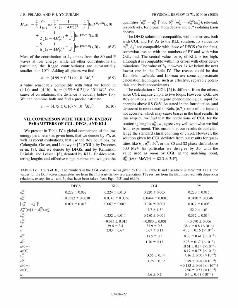
J. R. PELAEZ AND F. J. YNDURAIN PHYSICAL REVIEW D 71, 074016 (2005)
M�b1 �2
3
Z 1
4M2�
ds�1
3
�1
�s� 4M2��
3 �1
s3
�ImF�It�0��s; 0�
1
2
�1
�s� 4M2��
3 1
s3
�ImF�It�1��s; 0�
�5
6
�1
�s� 4M2��
3 �1
s3
�ImF�It�2��s; 0�
�: (6.8)
Most of the contribution to b1 comes from the S0 and Pwaves at low energy, while all other contributions (inparticular, the Regge contributions) are substantiallysmaller than 10�3. Adding all pieces we find
b1 � �4:99� 0:21� � 10�3M�5� ; (6.9)
a value reasonably compatible with what we found in(4.1a) and (4.1b), b1 � �4:55� 0:21� � 10�3M�5
� (be-cause of correlations, the distance is actually below 1�).We can combine both and find a precise estimate,
b1 � �4:75� 0:16� � 10�3M�5� : (6.10)
VII. COMPARISON WITH THE LOW ENERGYPARAMETERS OF CGL, DFGS, AND KLL
We present in Table IV a global comparison of the lowenergy parameters as given here, that we denote by PY, aswell as recent evaluations, that use the Roy equations, byColangelo, Gasser, and Leutwyler [2] (CGL), by Descoteset al. [8], that we denote by DFGS, and by Kaminski,Lesniak, and Loiseau [8], denoted by KLL. Besides scat-tering lengths and effective range parameters, we give the
TABLE IV. Units of M�. The numbers in the CGL column are asvalues for the D, F waves parameters are from the Froissart-Gribov rerelations, except for a1 and b1 that have been taken from Eqs. (6.3)
DFGS KLL
a�0�0 0:228� 0:032 0:224� 0:0
a�2�0 �0:0382� 0:0038 �0:0343� 0:
�a�0�0 � a�2�0 �2 0:071� 0:018 0:067� 0:0
��0�0 �m2
K� � ��2�0 �m2K�
b�0�0 0:252� 0:0
b�2�0 �0:075� 0:a1 39:6� 2:4b1 2:83� 0:6
a�0�2
a�2�2
a�0 �
a�00�b�0�2
b�2�2
b�0 �
b�00�a3
074016
quantities �a�0�0 � a�2�0 �2 and ��0�0 �m2
K� � ��2�0 �m2
K�, relevant,respectively, for pionic atom decays and CP violating kaondecays.
The DFGS solution is compatible, within its errors, bothwith CGL and PY. As to the KLL solution, its values fora�I�0 , b�I�0 are compatible with those of DFGS (for the first),somewhat less so with the numbers of PY and with whatCGL find. The central value for a1 of KLL is too high,although it is compatible within its errors with other deter-minations. The value of b1, however, is 3� below the nextlowest one in the Table IV. The reason could be thatKaminski, Lesniak, and Loiseau use some approximatecalculation techniques, such as effective, separable poten-tials and Pade approximants.
The calculation of CGL [2] is different from the others,since CGL impose ch.p.t. to two loops. However, CGL useRoy equations, which require phenomenological input forenergies above 0.8 GeV. As stated in the Introduction (anddiscussed in more detail in Refs. [6,7]) some of this input isnot accurate, which may cause biases in the final results. Inthis respect, we find that the predictions of CGL for thescattering lengths a�I�0 ; a1 agree very well with what we findfrom experiment. This means that our results do not chal-lenge the standard chiral counting of ch.p.t. However, thesolution given by CGL deviates from our results for quan-tities like b1, a�I�2 , b�I�2 , or the S0 and S2 phase shifts above500 MeV [in particular we disagree by 3� with thevalue used as input by CGL at the matching point,��0�0 ��800 MeV�2� � 82:3� 3:4o].
given by CGL in Table II and elsewhere in their text. In PY, thepresentation. The rest are from the fits, improved with dispersionand (6.10).
CGL PY
13 0:220� 0:005 0:230� 0:015
0036 �0:0444� 0:0010 �0:0480� 0:0046
07 0:070� 0:003 0:077� 0:008
47:7� 1:5� 52:9� 1:6�
11 0:280� 0:001 0:312� 0:014
015 �0:080� 0:001 �0:090� 0:00637:9� 0:5 38:4� 0:8 ��10�3�
7 5:67� 0:13 4:75� 0:16 ��10�3�
17:5� 0:3 18:70� 0:41 ��10�4�
1:70� 0:13 2:78� 0:37 ��10�4�
10:61� 0:14 ��10�4�
16:17� 0:75 ��10�4�
�3:55� 0:14 �4:16� 0:30 ��10�4�
�3:26� 0:12 �3:89� 0:28 ��10�4�
�0:183� 0:061 ��10�4�
�7:96� 0:57 ��10�4�
5:6� 0:2 6:3� 0:4 ��10�5�
-22
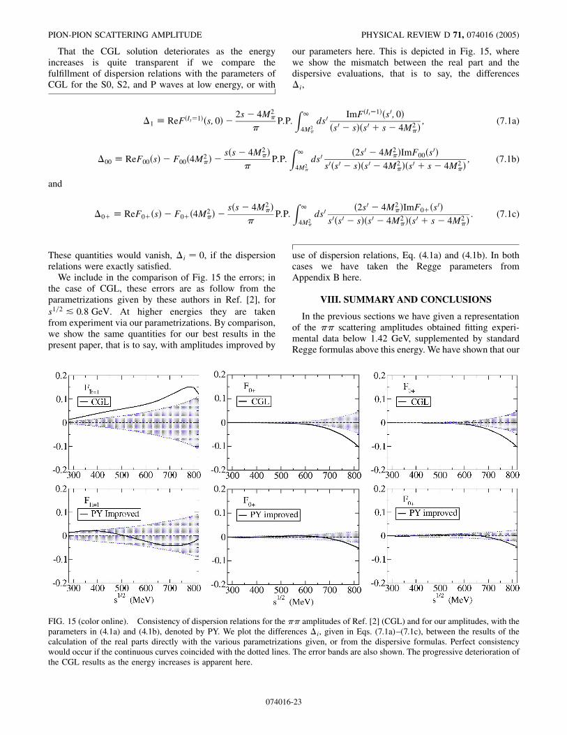
PION-PION SCATTERING AMPLITUDE PHYSICAL REVIEW D 71, 074016 (2005)
That the CGL solution deteriorates as the energyincreases is quite transparent if we compare thefulfillment of dispersion relations with the parameters ofCGL for the S0, S2, and P waves at low energy, or with
FIG. 15 (color online). Consistency of dispersion relations for the �parameters in (4.1a) and (4.1b), denoted by PY. We plot the differecalculation of the real parts directly with the various parametrizatiwould occur if the continuous curves coincided with the dotted lines.the CGL results as the energy increases is apparent here.
074016
our parameters here. This is depicted in Fig. 15, wherewe show the mismatch between the real part and thedispersive evaluations, that is to say, the differences�i,
�1 � ReF�It�1��s; 0� �2s� 4M2
�
�P:P:
Z 1
4M2�
ds0ImF�It�1��s0; 0�
�s0 � s��s0 s� 4M2��; (7.1a)
�00 � ReF00�s� � F00�4M2�� �
s�s� 4M2��
�P:P:
Z 1
4M2�
ds0�2s0 � 4M2
��ImF00�s0�
s0�s0 � s��s0 � 4M2���s0 s� 4M2
��; (7.1b)
and
�0 � ReF0 �s� � F0 �4M2�� �
s�s� 4M2��
�P:P:
Z 1
4M2�
ds0�2s0 � 4M2
��ImF0 �s0�
s0�s0 � s��s0 � 4M2���s0 s� 4M2
��: (7.1c)
These quantities would vanish, �i � 0, if the dispersionrelations were exactly satisfied.
We include in the comparison of Fig. 15 the errors; inthe case of CGL, these errors are as follow from theparametrizations given by these authors in Ref. [2], fors1=2 & 0:8 GeV. At higher energies they are takenfrom experiment via our parametrizations. By comparison,we show the same quantities for our best results in thepresent paper, that is to say, with amplitudes improved by
use of dispersion relations, Eq. (4.1a) and (4.1b). In bothcases we have taken the Regge parameters fromAppendix B here.
VIII. SUMMARY AND CONCLUSIONS
In the previous sections we have given a representationof the �� scattering amplitudes obtained fitting experi-mental data below 1.42 GeV, supplemented by standardRegge formulas above this energy. We have shown that our
� amplitudes of Ref. [2] (CGL) and for our amplitudes, with thences �i, given in Eqs. (7.1a)–(7.1c), between the results of theons given, or from the dispersive formulas. Perfect consistencyThe error bands are also shown. The progressive deterioration of
-23

J. R. PELAEZ AND F. J. YNDURAIN PHYSICAL REVIEW D 71, 074016 (2005)
representations satisfy reasonably well forward dispersionrelations at low energy, as well as crossing sum rules. Wehave shown that requiring fulfillment of the dispersionrelations up to s1=2 � 0:925 GeV leads to a refinement ofthe central values and errors for the parameters for thevarious waves, giving a set of these quantities such thatdispersion relations are now satisfied, within acceptableerrors, at all energies.
In particular, for the S0 wave, we have analyzed theresults found starting from different sets of data. If weeliminate from those sets the ones that are less consistentwith the dispersion relations, it is seen that the remainingdeterminations converge to a solution, essentially unique,when improved by requiring fulfillment of the dispersionrelations. We have, therefore, obtained a complete set of�� scattering amplitudes that are consistent, with theo-retical requirements as well as with experiment: they arecollected in Appendix A.
After this, we use these scattering amplitudes to evaluatelow energy parameters for P, D0, D2, and F waves in areliable manner, clearly improving on previous work.[1,2,8] These parameters may then be used to test chiralperturbation theory to one and two loops, or to find quan-tities relevant for pionium decays or CP violating kaondecays:
�a�0�0 � a�2�0 �2 � 0:077� 0:008M�2� ;
��0�0 �m2K� � ��2�
0 �m2K� � 52:9� 1:6o:
We may remark here that our errors are, typically, afactor 2 to 3 times larger than those in CGL, [2] at lowenergy. Given that the scattering amplitudes of this refer-ence show mismatches between high and low energy, formany observables by several standard deviations (cf., forexample, Fig. 15), and that our results are of higher preci-sion at intermediate energies for some quantities (compare,for example, the error bars in Figs. 15), we do not considerour results to be inferior. But one certainly can ask thequestion whether it would be possible to improve on ourprecision. The answer is no, in the sense that our ampli-tudes agree, within errors, with theoretical requirementsand with data. A sizable improvement would require sub-stantially improved experimental data, certainly for the S0,S2 waves at low energy, and for the S0 and P waves above1 GeV. One may think that imposing chiral perturbationtheory could lead to decreasing the errors of the ��scattering amplitudes. However, the matter is complicatedand will be left for a future publication.
ACKNOWLEDGMENTS
We are grateful to CICYT, Spain, and to INTAS,for partial financial support. We are also grateful toG. Colangelo and H. Leutwyler, whose questions aboutthe rho residue, 3"�t�, prompted us to give the alternatederivation and improvement of its values in Appendix B.
074016
APPENDIX A: SUMMARY OF LOW ENERGY(s1=2� 1:42 GeV) PARTIAL WAVES
In this appendix we collect the best values for theparametrizations of the various partial waves. We givethe values obtained after improving with the help of dis-persion relations, Eqs. (4.1a) and (4.1b). The values of theparameters and errors obtained from raw fits to data are asgiven in Sec. II.
1. The S wave with isospin zero below 950 MeV
We impose the Adler zero at s � 12 z
20, with z0 fixed, and
a ‘‘resonance’’ with mass +0, a free parameter. Afterimproving the global fit with dispersion relations we have
cot��0�0 �s� �s1=2
2kM2�
s� 12 z
20
+20 � s
+20
�B0 B1
���s
p�
�������������s0 � s
p
���s
p
�������������s0 � s
p
�;
B0 � 17:4� 0:5; B1 � 4:3� 1:4;
+0 � 790� 21 MeV; z0 � 195� 21 MeV �fixed�:
(A1)
This fit we take to be valid for s1=2 & 0:95 GeV. Note thatwe have fixed the value of z0 when evaluating the errors ofthe other parameters.
This gives
a�0�0 � �0:230� 0:015�M�1� ;
b�0�0 � �0:312� 0:014�M�3� ;
��0�0 �mK� � 44:4� � 1:5�:
(A2)
2. The I� 0 S wave between 950 MeV and 1420 MeV
We write
cot��0�0 �s� � c0�s�M2
s ��M2f � s�
M2fs
1=2
jk2j
k22;
k2 �
������������������s� 4m2
K
q2
; (A3)
��0�0 � 1�
'1
k2s1=2
'2k22s
M02 � s
s: (A4)
Then,
c0 � 1:3� 0:5; Mf � 1320� 50 MeV;
Ms � 920 MeV �fixed�; '1 � 6:4� 0:5;
'2 � �16:8� 1:6; M0 � 1500 MeV �fixed�:
(A5)
It should be clear that this fit is not very reliable since thereare several incompatible sets of experimental data. Thus,the errors are purely nominal. If using��! �KK data to fitthe inelasticity we would have obtained different values forthe 'i:
-24

PION-PION SCATTERING AMPLITUDE PHYSICAL REVIEW D 71, 074016 (2005)
'1 � 2:4� 0:2; '2 � �5:5� 0:8: (A50)
This fit has not been improved with dispersion relations.For dispersion relations below 0.925 GeV, it is irrelevantwhether we use (A5) or (A50).
3. Parametrization of the S wave for I� 2 below 1 GeV
We fit only the low energy data, s1=2 < 1:0 GeV, takingthe inelastic threshold at s0 � 1:052 GeV2,
cot��2�0 �s� �s1=2
2kM2�
s� 2z22
�B0 B1
���s
p�
�������������s0 � s
p
���s
p
�������������s0 � s
p
�;
s1=2 � 1:0 GeV: (A6)
The central values and errors are improved with dispersionrelations; we get
B0 � �80:8� 1:7; B1 � �77� 5;
z2 � 147� 7 MeV �fixed�;
a�2�0 � ��0:0480� 0:0046� �M�1� ;
b�2�0 � ��0:090� 0:006� �M�3� ;
��2�0 �m2
K� � �8:5� 0:3�:
(A7)
4. Parametrization of the S wave for I� 2 above 1 GeV
At high energy, we may fit data from s1=2 � 0:91 GeVup to s1=2 � 1:42 GeV. We require junction with the lowenergy fit at 1 GeV, neglect inelasticity below 1:45 GeV,and write
cot��2�0 �s� �s1=2
2kM2�
s� 2z22
�B0 B1
���s
p�
�������������s0 � s
p
���s
p
�������������s0 � s
p
�;
s1=20 � 1:45 GeV; z2 � 147 MeV �fixed�: (A8a)
After improving with dispersion relations we then find
B0 � �125� 6; B1 � �119� 14;
s > �1:0 GeV�2:(A8b)
The inelasticity may be described by the empirical fit
��2�0 �s� � 1� '�1� s=s�3=2; ' � 0:17� 0:12
�s1=2 � 1:05 GeV�:
These formulas are expected to hold from 1 GeV up to1:42 GeV.
5. The P wave below 1 GeV
We have
cot�1�s� �s1=2
2k3�M2
" � s��B0 B1
���s
p�
�������������s0 � s
p
���s
p
�������������s0 � s
p
�;
s1=20 � 1:05 GeV: (A9a)
074016
The best result, from (4.1a) and (4.1b), is
B0 � 1:064� 0:011; B1 � 0:170� 0:040;
M" � 773:6� 0:9; a1 � �38:7� 1:0� � 10�3M�3� ;
b1 � �4:55� 0:21� � 10�3M�5� : (A9b)
Slightly better values for a1, b1, improved with sum rules,may be found in Table IV.
6. The P wave for 1 GeV� s1=2� 1:42 GeV
For the P wave between 1 GeV and 1.4 GeV we use anempirical formula, obtained with a linear fit to the phaseand inelasticity of Protopopescu et al. [10] and Hyams etal. [11]
�1�s� � �0 �1��������s=s
p� 1�;
�1�s� � 1� '��������s=s
p� 1�; ' � �0:30� 0:15�;
�0 � 2:69� 0:01; �1 � 1:1� 0:2: (A10)
Here s � 1 GeV2. The value of �0 ensures the agree-ment of the phase with the value given by (A9a) and (A9b)at s � s � 1 GeV2. This fit is good; however, it should beremarked that there are other sets of experimental data forthis wave disagreeing with the one used here for s1=2 >1:15 GeV. Hence (A10) may be biased beyond its nominalerrors.
This fit has not been improved with dispersion relations.
7. Parametrization of the D wave for I� 0
We fit data on ��0�2 altogether neglecting inelasticity,which we will then add by hand. The data are scanty, andof poor quality. We impose in the fit the scattering length,as obtained from the Froissart-Gribov representation, andthe experimental width of the f2. Moreover, we improvethe central values with dispersion relations.
We write
cot��0�2 �s� �s1=2
2k5�M2
f2� s�M2
�fB0 B1w�s�g; (A11a)
and
w�s� �
���s
p�
�������������s0 � s
p
���s
p
�������������s0 � s
p ; s1=20 � 1450 MeV;
Mf2 � 1275:4 MeV �fixed�:
We find,
B0 � 23:5� 0:7; B1 � 24:8� 1:0: (A11b)
-25

J. R. PELAEZ AND F. J. YNDURAIN PHYSICAL REVIEW D 71, 074016 (2005)
We take into account the inelasticity by writing
��0�2 �s� �
� 1; s < 4m2K;
1� 'k2�s�k2�M
2f2�; ' � 0:262� 0:030; s > 4m2
K:
(A11c)
Here k2 ����������������������s=4�m2
K
q:
The fit returns the values
a�0�2 � �18:4� 3:0� � 10�4 �M�5� ;
b�0�2 � ��8:6� 3:4� � 10�4 �M�7� :
Better values for a�0�2 ; b�0�2 are given in Table IV.
8. Parametrization of the D wave for I� 2
For isospin equal 2, there are no resonances in the Dwave. If we want a parametrization that applies down tothreshold, we must incorporate the zero of the correspond-ing phase shift. So we write
cot��2�2 �s� �s1=2
2k5fB0 B1w�s� B2w�s�
2g
�M4�s
4�M2� �2� � s
;
s1=2 � 1:05 GeV:
(A12a)
with � a free parameter and
w�s� �
���s
p�
�������������s0 � s
p
���s
p
�������������s0 � s
p ; s1=20 � 1450 MeV:
Moreover, we impose the value for the scattering lengththat follows from the Froissart-Gribov representation. Weassume negligible inelasticity and find, after improvementwith dispersion relations,
B0 � �2:9� 0:2� � 103; B1 � �7:3� 0:8� � 103;
B2 � �25:4� 3:6� � 103; � � 212� 19 MeV:
074016
The fit returns reasonable values for the scattering lengthand effective range parameter, b�2�2 :
a�2�2 � �2:4� 0:7� � 10�4M��5;
b�2�2 � ��2:5� 0:6� � 10�4M��7:
(A13)
Better values for a�2�2 ; b�2�2 are given in Table IV.
9. The F wave
For the F wave below s1=2 � 1:42 GeV we fit the phaseshifts of Protopopescu et al. [10] and those of Hyams et al.[11(b)], plus the scattering length as given by the Froissart-Gribov representation. After honing the central values ofthe parameters with the help of dispersion relations we find
cot�3�s� �s1=2
2k7M6�
�B0 B1
���s
p�
�������������s0 � s
p
���s
p
�������������s0 � s
p
�;
B0 � �1:09� 0:03� � 105;
B1 � �1:41� 0:04� � 105:(A14)
This implies a3 � �7:0� 0:8� � 10�5M�7� , in agreement
(within errors) with the result of the Froissart-Gribov cal-culation (Table IV).
The contribution of the F wave to all our sum rules isvery small (but not always negligible); the interest ofcalculating it lies in that it provides a test (by its verysmallness) of the convergence of the partial waveexpansions.
10. The G waves
For the G0 wave, we take its imaginary part to be givenby the tail of the f4�2050� resonance, with its properties asgiven in the particle data tables:
Im f�0�4 �s� �k�s�
k�M2f4�
18BR
M2f4�2
�s�M2f4�2 M2
f4�2�k�s�=k�M2
f4��18
; s1=2 � 1 GeV; BR � 0:17� 0:02;
Mf4 � 2025� 8 MeV; � � 194� 13 MeV:
(A15)
For the wave G2, we can write, neglecting its eventualinelasticity,
cot��2�4 �s� �s1=2M8
�
2k9B; B � ��9:1� 3:3� � 106;
s1=2 � 1 GeV: (A16)
It should be noted that the expressions for the G0, G2waves, are little more than order of magnitude estimates.
Moreover, at low energies they certainly fail; below 1 GeV,expressions in terms of the scattering length approxima-tion, with
a�0�4 � �8:0� 0:4� � 10�6M�9� ;
a�2�4 � �4:5� 0:2� � 10�6M�9� ;
are more appropriate. If, in a given calculation, the con-tribution of either of the 2 G waves is important, it means
-26

PION-PION SCATTERING AMPLITUDE PHYSICAL REVIEW D 71, 074016 (2005)
that the calculation will have a large error. We havechecked in a representative number of our calculationsthat the contributions of the G0, G2 waves are totallynegligible.
APPENDIX B: THE REGGE AMPLITUDE(s1=2� 1:42 GeV)
In the calculations of the various sum rules and disper-sion relations we require the imaginary part of the scatter-ing amplitudes at high energy. For this we use Reggeformulas, applicable when s� .2, with . ’ 0:3 GeVthe QCD parameter, and s� jtj. Specifically, we usethem above s1=2 � 1:42 GeV and expect them to be validat least for jtj & 4M2
� ’ 0:08 GeV2. These formulas areobtained from NN, �N scattering, using factorization, andfrom direct fits to�� data. We will not include refinementsthat take into account the logarithmic increase of totalcross sections at ultrahigh energies (that may be found inRef. [5]), superfluous for applications to�� scattering. Wegive here the relevant formulas, for ease of reference, forPomeron and P0 Regge poles, and will only discuss in somedetail (and even improve slightly) the parameters of the rhoresidue.
We consider three Regge poles: Pomeron (P), the P0
[associated with the f2�1270� resonance] and the rho. Forthe first two,
ImF�It�0��� �s; t� ’
s!1t fixed
P�s; t� P0�s; t�;
P�s; t� � 3P4P�t�1 4P�t�
2ebt�s=s�4P�t�;
P0�s; t� � 3P0
4P0 �t��1 4P0 �t��4P0 �0��1 4P0 �0��
ebt�s=s�4P0 �t�;
4P0 �t� � 4"�t�: (B1)
For exchange of unit isospin, we write
ImF�It�1��� �s; t� ’
s!1t fixed
"�s; t�; "�s; t� � 3"�t��s=s�4"�t�:
(B2a)
In the present paper we have taken a formula slightlydifferent from that in Ref. [5], viz.,
3"�t� � 3"�0�1 4"�t�
1 4"�0��1 d"t�ebt ’
t!03"�0��1 c"t�;
c" � b d" 40"�0�
1 4"�0�: (B2b)
In Ref. [5], where we took an expression from Rarita et al.[18], solution 1a, assuming the t dependence to be equal for�� and �N scattering [see below, Eq. (B7)]. Our expres-sion now, (B2b), is simpler. As we will show below, we can
074016
fix its parameters (for small values of t) without assumingthe equality of �� and �N.
For exchange of isospin two,
ImF�It�2��� �s; t� ’
s!1t fixed
R2�s; t� � 32ebt�s=s�4"�t� 4"�0��1:
(B3)
This last amplitude corresponds to double rho exchange;the expression we use for it at t � 0 is rather arbitrary,since little is known about it. Fortunately, it has almost noinfluence in the calculations.
Following the analysis of Ref. [5], the trajectories aretaken as follows:
4P�t� ’t04P�0� 40
Pt; 4"�t� ’t04"�0� 40
"t 1
2400"t2;
(B4)
and one has
4"�0� � 0:52� 0:02; 40" � 0:90 GeV�2;
400" � �0:3 GeV�4; 4P�0� � 1;
40P � �0:20� 0:10� GeV�2:
(B5)
Moreover, in the present paper, we have taken the follow-ing values for the parameters of the residues:
3P � 2:54� 0:03; 3P0 � 1:05� 0:02;
32 � 0:2� 0:2; b � �2:4� 0:2� GeV�2;
3" � 3"�0� � 1:02� 0:11; d" � �2:4� 0:9� GeV�2:
(B6)
The parameters for P, P0 are like in Ref. [5]. Those for therho trajectory are as improved below.
The Pomeron and P0 parameters are well fixed fromfactorization and (besides �� cross sections) by �N, NNdata, down to kinetic energies ’ 1 GeV; but some extrawords will be added on the rho residue, 3"�t�. This quan-tity was obtained in Ref. [5] in a mixed manner: 3" �
3"�0� was found fitting high energy �� data, improvingthe error with the help of the sum rule (5.2). The t depen-dence of 3"�t� was taken as in solution 1a of Rarita et al.[18] assuming it to be identical for �� and �N scattering.Thus, we wrote
3"�t� � 3"�0���1:5 1�ebt � 1:5�
�1 4"�t�
1 4"�0�’t!03"�0��1 c"t�;
c" � 2:5b 40"�0�
1 4"�0�:
(B7)
This, in fact, is similar to (B2b) and (B6) for small valuesof jtj, as we will check below.
There are other possibilities for the t dependence of therho residue. We could have chosen solution 1 of Rarita et
-27

-0.2 -0.4 -0.6+0.2
-0.5
-1.0
-0.5
-0
4M2π
t (GeV)2
(Rarita et al., solution 1)
(Rarita et al., solution 1a)
(Froggatt & Petersen)
(Palou&Yndurain; diff. factor)
FIG. 16. The t dependence of the different Regge residues,3�t�=3�0� (Refs. [18,19]): Rarita et al., solution 1 and solution1a: the fits from Rarita et al. (assuming equal slope for �N and��). Froggatt and Petersen: from fits to �� dispersion relationsat fixed t. Palou and Yndurain; diffraction factor: actually, fromthe Veneziano model, including a diffraction factor ebt; b �2:4 GeV, as in Eq. (B7). The residue given in (B6) would liebetween ‘‘Palou and Yndurain diffraction factor’’ and ‘‘Rarita etal. solution 1a’’ (closer to the second).
J. R. PELAEZ AND F. J. YNDURAIN PHYSICAL REVIEW D 71, 074016 (2005)
al. [18] or we could have taken a Veneziano-type formulawith a diffractive factor included, writing
"�s; t� � 3"�t��s=s�4"�t�;
3"�t� � 3"�0���1� 4"�t�� sin�4"�t�
��1� 4"�0�� sin�4"�0�
� ebt ’t!03"�0��1 c"t�;
c" ’ b 6E40"�0�:
(B8)
Another possibility is afforded by the t dependence ob-tained by Froggatt and Petersen [19] from an analysis of� �� dispersion relations at fixed t. These authors take
3"�t� � 3"�0�sin�4"�t�
sin�4"�0��1� t=t"�e
bFPt; (B9)
with t�1" � �2:2 GeV�2, bFP � 0:8 GeV�2. This gives a
slope for the residue of about half the value of solution 1aof Rarita et al.
The values of 3"�t�, both 3"�0� and t dependence, aregiven by Regge fits with less precision than other quanti-ties; a few determinations (including the ones mentionedhere) are shown in Fig. 16. The variation from one estimateto another in the range necessary for Roy equations, �t ’0:6 GeV2, is very large, and even at jtj ’ 0:1 GeV2 thereare noticeable differences.
Fortunately, we can at least check the correctness(within errors) of the values of 3"�t� given in Ref. [5] att � 0 and t � 4M2
� ’ 0:08 GeV2, and even improvethem. In fact, apart from the sum rule (5.2), the fulfillmentof the dispersion relation (3.5) fixes with good accuracy3"�0�, and combinations of both values 3"�0� and3"�4M
2�� enter in the evaluations, using the Froissart-
Gribov representation, of two quantities, a1, b1, thatcan also be determined by other methods, independent ofthe Regge assumptions. The ensuing equality of the twoestimates each for a1, b1 given in Eqs. (6.2) and (6.4)fixes c", as we will see below. Thus, if, for example,we had taken the Veneziano-type t dependence of Palouand Yndurain [19] [i.e., as in (B8) without the exponentialfactor ebt) we would have obtained b1 3� 10�3M�5
� ,quite incompatible with determinations from the pionform factor or the sum rule (6.8). Even if we include adiffraction factor as in (B8), the values of a1, b1 followingfrom the Froissart-Gribov representation vary by morethan 1�.
074016
One can in principle fix the parameters for ��scattering from other processes profiting from factoriza-tion, which allows one to improve the poor precision of the�� data. This is all right for the P, P0 poles because herewe can use data from �N and �pp pp, scattering whichare very precise and to which only these two poles, plus therho pole for �N, contribute. The situation is different forthe coupling of the rho pole to ��. Direct fits to �� dataare not precise and, to use factorization, one has to incor-porate (besides �N) proton, antiproton and neutron scat-tering data. The last presents important systematic errorsbecause the data have to be extracted from scattering ondeuterons. The large number of trajectories that contributeto these processes also make the analysis unreliable; forexample, some existing fits have very likely their rhotrajectory contaminated by pion exchange, which is notnegligible at the lower energy range. Because of this, wewill now give a new determination of 3"�0� and d" inde-pendent of Regge fits.
To obtain 3"�0�, we rewrite the dispersion relation (3.7)as
ReF�It�1��s;0� �2s� 4M2
�
�P:P:
Z 1:422 GeV2
4M2�
ds0ImF�It�1��s0;0�
�s0 � s��s0 s� 4M2��
�2s� 4M2
�
�
Z 1
1:422 GeV2ds0
ImF�It�1��s0;0�
�s0 � s��s0 s� 4M2��:
(B10)
We evaluate the left hand side for values of s1=2 from threshold to 925 MeV, at intervals of 25 MeV, using low energy
-28

PION-PION SCATTERING AMPLITUDE PHYSICAL REVIEW D 71, 074016 (2005)
experimental data, via the parametrizations6 given in Sec. II. In this region, s1=2 � 0:925 GeV, the uncertainties due to themiddle energy S0 and P waves are not very important. If we write in the right hand side of (B10)
ImF�It�1��s0; 0� � 3"�0��s0=s�4"�0�; s � 1:422 GeV2;
and fix 4"�0� � 0:52 from factorization or deep inelastic scattering, we may fit 3"�0� and find a very precise number,
3"�0� � 1:06� 0:10: (B11)
This is quite compatible with the value 3"�0� � 0:94� 0:14 that we obtained from fits to �� cross sections in Ref. [5].The result (B11) is robust; if we double the errors of the parameters for the P and S0 waves between 1 and 1.42 GeV, where(as discussed in the main text) one has larger uncertainties, and repeat the fit, we get the same value.
As for c", we can use the values of a1, b1 obtained from the analysis of the pion form factor [9], together with theFroissart-Gribov representation of the same quantities. We rewrite Eq. (6.1) as
a1 �
�����
p��2�
4M���1 3=2�
Z 1:422 GeV2
4M2�
dsImF�It�1��s; 4M2
��
s3�
�����
p��2�
8M���1 3=2�
Z 1
1:422 GeV2ds
ImF�It�1��s; 4M2��
s3: (B12a)
For the bl, l � odd,
bl �
�����
p��l 1�
4M���l 3=2�
Z 1:422 GeV2
4M2�
ds�4ImF�It�1�0 �s; 4M2
��
�s� 4M2��s
l 1�
�l 1�ImF�s; 4M2��
sl 2
�
�
�����
p��l 1�
4M���l 3=2�
Z 1
1:422 GeV2ds�4ImF�It�1�0 �s; 4M2
��
�s� 4M2��sl 1
��l 1�ImF�s; 4M2
��
sl 2
�;
ImF�It�1�0 �s; t� � @ImF�It�1��s; t�=@ cos�:
(B12b)
The left hand sides in (B12a) and (B12b) are evaluatedusing also the experimental phase shifts and inelasticitiesas fitted in Sec. II of the present paper and we take, in theright hand side of (B12a),
ImF�It�1��s; 4M2�� � 3"�4M
2���s=s�
4"�4M2��;
s � 1:422 GeV2;
3"�t� ’ 3"�0��1 c"t�: An analogous formula may bewritten for the right hand side of (B12b). The sum rulefor b1 gives the more precise constraint for c" for tworeasons. First, it depends directly on the derivative ofImF�It�1��s; t� with respect to t ( cos�), hence c" appearsexplicitly; and, second, the low energy contributions to theleft hand side in (B12b) cancel to a large extent, so b1 isgiven almost exclusively by the high energy, Regge for-mulas; cf. Ref. [6].
6Of course, before improving with dispersion relations, or thereasoning would be somewhat circular. Alternatively, we couldfit simultaneously the parameters for phase shifts and inelastic-ities and the Regge parameters of the rho, using all threedispersion relations; the method, quite complicated, would notgive results substantially different from what we get makingindependent fits.
074016
We can fit, with these sum rules for a1, b1, plus thedispersion relation for It � 1, the parameters 3"�0�, c"simultaneously. As was to be expected, the value of 3"�0�is unchanged and, for c", we find the values
c" �
��6:0� 2:8� GeV�2 from a1;�4:7� 0:8� GeV�2 from b1:
(B13)
This is compatible with what one has from solution 1a ofRarita et al. [18], c" � �6:6� 0:5� GeV�2 in the sense thatthey produce similar values for 3"�4M2
��: the decrease inc" is compensated (within errors) by the increase in 3"�0�,Eq. (B1), compared with what we used in Ref. [5]. Ourresults for c" thus justify the use of the formulas of solution1a of Rarita et al. [18], for small values of jtj & 0:1 GeV,as was done in Ref. [6], and the assumption that (in thatrange) they are also valid for �� scattering, within errors.
We can also include in the fit the information from ��scattering data (as discussed in Ref. [5]), since it is com-patible with what we found now, and the sum rule (5.2),evaluated with the parameters found in Sec. II here for thelow energy piece. In this case we find what we consider thebest results,
-29
J. R. PELAEZ AND F. J. YNDURAIN PHYSICAL REVIEW D 71, 074016 (2005)
3"�0� � 1:02� 0:11; c" � �5:4� 0:9� GeV�2:
(B14a)
This implies
d" � �2:4� 0:9� GeV�2: (B14b)
Equations (B14a) and (B14b) provide us with the centralvalues given in (B6) for d", 3"�0�.
APPENDIX C: ON EXPERIMENTAL PHASESHIFTS IN THE RANGE 1:4 GeV’ s1=2’ 2 GeV
As is well known, as soon as the center of mass kineticenergy in a hadronic reaction, Ekin;c:m:, increases beyond1 GeV, inelastic processes become important and, forEkin;c:m: * 1:3 GeV, they dominate elastic ones. This iseasily understandable in the QCD, ladder version of theRegge picture, as discussed in Ref. [6]; and indeed, it isverified experimentally in the hadronic processes �N, KN,and NN where, for Ekin;c:m: > 1:3 GeV, the elastic crosssection is smaller than the inelastic one and, for Ekin;c:m: >1:5 GeV, the elastic cross section is less than or about onehalf of the inelastic one. There is no reason to imagine that�� scattering would follow a different pattern. In this case(large inelasticity), and again as mentioned in Refs. [6,7], itcan be proved theoretically [20] that there is not a uniquesolution to the phase shift analysis: some sets of �s and �smay fit the data; but so would others.
In spite of this, the Cern-Munich experiments7
have produced a set of phase shifts and inelasticities whichgo up to s1=2 ’ 2 GeV. These have been used as input incertain theoretical analyses, notably in those of Refs. [1,2].Unfortunately, such phase shifts and inelasticities are verylikely to diverge more and more from reality as s1=2
becomes larger and larger than 1:3 GeV ’ 2M� 1 GeV. This is suggested, besides the theoretical reasonsjust mentioned, by the fact that the Cern-Munich phaseshifts and inelasticities contradict a number of physicalproperties they should fulfill: we will here mention a few.
As we have remarked above, one would expect domi-nant inelastic cross sections above s1=2 1:5 GeV; but theCern-Munich elastic cross sections are larger or compa-rable to the inelastic ones up to s1=2 � 2 GeV. What isworse, the � �� inelastic cross section of Cern-Munich,alone of all hadronic cross sections, decreases as thekinetic energy increases between 1 and 1.7 GeV, as shown,for example, in Fig. 7 in the paper of Hyams et al. [11(a)].As happens for 6N,�N,KN, orNN scattering, and indeedas is also seen in other experimental analyses for ��scattering [4], we expect a leveling off of the total crosssection for Ekin;c:m: > 1:3 GeV: but the Cern-Munich totalcross section for � �� scattering decreases roughly like
7Hyams et al. and Grayer et al., Refs. [11(a),11(b)].
074016
1=s up to 2 GeV. In fact, the Cern-Munich elastic crosssection agrees well with that found in other experiments(such as those in Ref. [4]), but their total cross section issmaller by a factor 2 than those in Refs. [4], at the higherpart of the energy range: the Cern-Munich results certainlymisrepresent the total cross section. From all this it followsthat the Cern-Munich phases and inelasticities are notreliable in that energy region.
Second, the combination of � and � for both P and S0waves at energy * 1:8 GeV is incompatible with QCDresults for the electromagnetic form factor of the pion,and also with Regge behavior, which requires all phasesto go to a multiple of � at high energy, and the real part ofthe partial wave amplitudes for isospin 0, 1, to be positive.The phase �1 is also incompatible with QCD results for theelectromagnetic form factor of the pion. In fact, the phaseof this form factor behaves like
�form factor�s� ’ �1
1
logs=t
; s� .2; t.2;
. is the QCD parameter (see, e.g., Ref. [21]). One maytake this to hold for s * 3 GeV2 (s1=2 > 1:6 GeV). If onehad negligible inelasticity for the P wave somewhere in theregion 1:6 GeV & s1=2 & 2 GeV, as the Cern-Munich dataseem to imply, the form factor and partial wave would havethe same phase at such energies, and thus the same behav-ior should hold for �1�s�, �form factor�s�. But the phasewhich the Cern-Munich experiment gives clearly contra-dict this behavior around 1:8 GeV; there the Cern-Munichphase �1 stays consistently below �, while, as just shown,it should be above.
Third, for the process ���� ! ����, we would ex-pect large inelasticity as soon as the production ���� !"�"� is energetically possible, and therefore large inelas-ticity for the S2, D2 waves for s1=2 � 2M". This, inparticular, occurs in any theoretical model. It is thereforenot possible to extrapolate these phases above 1:45 GeVas being elastic. In fact, the extrapolation used inRefs. [1,2] for the D2 wave is clearly incorrect above1:4 GeV as the corresponding j��2�2 �s�j grows linearlywith swhile, from Regge theory (and also from low energyfits, see Fig. 7), one expects it to go to zero. Thus, besidesthe general problem for the cross sections we have indi-vidual problems for each of the S0, S2, P, and D2 phases.
Finally we would like to mention that both the Reggepicture and the values of the experimental cross sectionsfor all hadronic processes indicate that the number ofwaves that contribute effectively to the imaginary part(say) of the scattering amplitudes grows with the kineticenergy as Ekin=., for Ekin upwards of 1 GeV . We thusexpect 2 to 3 waves (for fixed isospin) at Ekin 1 GeV,and almost double this, 4 or 5 waves, at Ekin 1:7 GeV. Infact, for�� scattering at this energy, the contribution to thetotal cross section of the F wave is as large as that of the P
-30

8We would like to emphasize that what has been said shouldnot be taken as implying criticism of the Cern-Munich experi-ment which, for s1=2 & 1:4 GeV, produced what are probably thebest determinations of phase shifts and inelasticities. Above1:4 GeV, they did what they could: it is for theorists to realizethat this was not enough to produce acceptable phase shifts andinelasticities at these higher energies.
PION-PION SCATTERING AMPLITUDE PHYSICAL REVIEW D 71, 074016 (2005)
wave, the D0 wave is as large as the S0 wave and thecontribution of the D2 wave is actually larger than that ofthe S2 wave. The partial wave series with only two wavesper isospin channel is not convergent, and the approxima-tions, like those of Refs. [1,2,11], that neglect higher wavesat such energies have yet another reason for being unreal-istic [14].
Because of all this, it follows that use of the Cern-Munich phases and inelasticities must lead to a ratherdistorted imaginary part of the �� scattering amplitudeabove s1=2 1:4 GeV. It is thus not surprising that authorslike those in Refs. [1,2,15], who fix their Regge parameters
074016
by balancing them above 2 GeV with Cern-Munich phaseshift analyses below 2 GeV, get incorrect values for thefirst.8
[1] B. Ananthanarayan et al., Phys. Rep. 353, 207(2001).
[2] G. Colangelo, J. Gasser, and H. Leutwyler, Nucl. Phys.B603, 125 (2001).
[3] S. M. Roy, Phys. Lett.36B, 353 (1971).[4] N. N. Biswas et al., Phys. Rev. Lett. 18, 273 (1967)
[����, � ��, and �0��]; D. Cohen et al., Phys. Rev.D 7, 661 (1973) [����]; W. J. Robertson, W. D. Walker,and J. L. Davis, Phys. Rev. D 7, 2554 (1973) [� ��]; W.Hoogland et al., Nucl. Phys. B126, 109 (1977) [����]; J.Hanlon et al., Phys. Rev. Lett. 37, 967 (1976) [� ��]; H.Abramowicz et al., Nucl. Phys. B166, 62 (1980) [� ��].These references cover the region between 1.35 and16 GeV, and agree within errors in the regions wherethey overlap (with the exception of ���� below2.3 GeV, discussion in Ref. [5]).
[5] J. R. Pelaez and F. J. Yndurain, Phys. Rev. D 69, 114001(2004).
[6] J. R. Pelaez and F. J. Yndurain, Phys. Rev. D 68, 074005(2003).
[7] F. J. Yndurain, hep-ph/0310206.[8] S. Descotes, N. H. Fuchs, L. Girlanda, and J. Stern, Eur.
Phys. J. C, 24, 469 (2002); R. Kaminski, L. Lesniak, andB. Loiseau, Phys. Lett. B 551, 241 (2003).
[9] J. F. de Troconiz and F. J. Yndurain, Phys. Rev. D 65,093001 (2002); hep-ph/0402285 [Phys. Rev. D (to bepublished)]. When quoting numbers, we will quote fromthis last paper.
[10] S. D. Protopopescu et al., Phys. Rev. D 7, 1279 (1973).[11] The Cern-Munich experiments (�� scattering). (a) B.
Hyams, Nucl. Phys. B64, 134 (1973); G. Grayer et al.,Nucl. Phys. B75, 189 (1974); see also the analysis of the
same experimental data in P. Estabrooks and A. D. Martin,Nucl. Phys. B79, 301 (1974). (b) B. Hyams et al., Nucl.Phys. B100, 205 (1975). (c) R. Kaminski, L. Lesniak, andK. Rybicki, Z. Phys. C 74, 79 (1997); Eur. Phys. J. direct C4, 4 (2002). ��! KK scattering: (d) W. Wetzel et al.,Nucl. Phys. B115, 208 (1976); V. A. Polychromatos et al.,Phys. Rev. D 19, 1317 (1979); D. Cohen et al., Phys. Rev.D 22, 2595 (1980); E. Etkin et al., Phys. Rev. D 25, 1786(1982).
[12] M. J. Losty et al., Nucl. Phys. B69, 185 (1974); W.Hoogland et al., Nucl. Phys. B126, 109 (1977); N. B.Durusoy et al., Phys. Lett. B 45, 517 (1973).
[13] L. Rosselet et al., Phys. Rev. D 15, 574 (1977); S. Pislaket al., Phys. Rev. Lett. 87, 221801 (2001).
[14] For the more recent determination, see A. Aloisio et al.,Phys. Lett. B 538, 21 (2002); an older one is P. Pascual andF. J. Yndurain, Nucl. Phys. B83, 362, (1974).
[15] M. R. Pennington, Ann. Phys. (N.Y.) 92, 164 (1975).[16] B. R. Martin, D. Morgan, and G. Shaw, Pion-Pion
Interactions in Particle Physics (Academic Press, NewYork, 1976).
[17] F. P. Palou, J. L. Sanchez-Gomez, and F. J. Yndurain, Z.Phys. A 274, 161 (1975).
[18] W. Rarita et al., Phys. Rev. 165, 1615 (1968).[19] C. D. Froggatt and J. L. Petersen, Nucl. Phys. B129, 89
(1977); F. P. Palou and F. J. Yndurain, Nuovo Cimento19A, 245 (1974).
[20] D. Atkinson et al., Nucl. Phys. B7, 375 (1968); Nucl.Phys. B23, 397 ( 1970).
[21] F. J. Yndurain, Phys. Lett. B 578, 99 (2004); Phys. Lett. B586, 439(E) (2004); hep-ph/0501104 [Phys. Lett. B (to bepublished)].
-31