1

Physics 509: PropagatingSystematic Uncertainties

Scott OserLecture #12

Physics 509 2

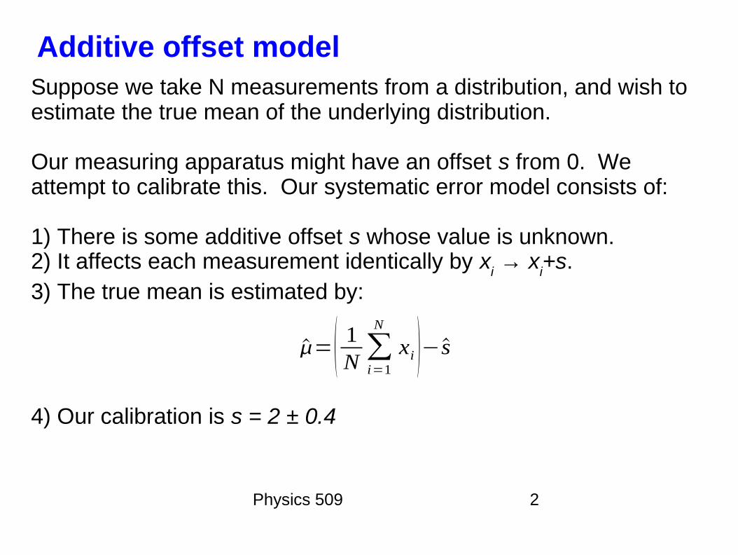
Additive offset modelSuppose we take N measurements from a distribution, and wish to estimate the true mean of the underlying distribution.

Our measuring apparatus might have an offset s from 0. We attempt to calibrate this. Our systematic error model consists of:

1) There is some additive offset s whose value is unknown.2) It affects each measurement identically by x

i → x

i+s.

3) The true mean is estimated by:

4) Our calibration is s = 2 ± 0.4

= 1N∑i=1

N

xi −s

Physics 509 3

Covariance solution to additive offset model 1We start by assembling the covariance matrix of the data:

cov(xi,x

j) =

ij

i2 +

s2

V ij= [1

2 s

2 s

2 s

2 s

2

s2

22 s

2 s

2 s

2

s2

s2

32 s

2 s

2

s2

s2

s2

42 s

2 ]Next we form the likelihood (or 2) using this covariance matrix:

2=∑

i∑j

xi−−sV ij−1x j−−s

The ML (LS) estimator is that which minimizes the 2.

Physics 509 4

Covariance solution to additive offset model 2

2=∑

i∑j

xi−−sV ij−1x j−−s

I calculated this for

xi = (10,12,10,11)

i = 1

s = 0.4

Result = 8.75 ± 0.64

s=2

Physics 509 5

You've got to be kidding me ...By now most of you must have realized that nobody calculates errors this way. The more usual approach is:

1) Calculate the central value and its statistical error:

2) Calculate the systematic error on the parameter due to the uncertainty in s. Since we said s=2.0±0.4, and we can think of and so apply error propagation to get the systematic.

= 1N∑i=1

N

xi −s=8.75±1.04

=8.75±0.5

= s∣xi

=8.75±0.5±0.4=8.75±0.520.42

=8.75±0.64

Systematic error propagation by the “” methodAll of these suggests a simple way to propagate uncertainties for a parameter estimator. Let ĝ=ĝ(x

i|s

1,s

2, ...) be a function of the

data x2 and a set of systematics parameters.

Calculate the parameter estimate and its statistical uncertainty, keeping all of the systematics fixed, by the usual methods. Vary each systematic (nuisance parameter) one by one by ±1, and note the change in ĝ. In other words, calculate ĝ

1=ĝ(x

i|s

1±

1,s

2, ...) - ĝ(x

i|s

1,s

2, ...)

Combine the various uncertainties using error propagation: g = ĝ + ĝ

stat + ĝ

1+ ĝ

2+ ...

Finally, add up systematics in quadrature to get

gsys= g12 g2

2...

(If any systematics are correlated, include correlation coefficients as well.)

gsys= g12 g2

2 g1 g2...

Physics 509 7

An example of the method: linear fit with distorting systematicsSuppose our model predicts y=mx+b, and we wish to estimate m and b. Each measurement has dy=1. For a particular set of data:

Best fit: m = 0.46±0.12, b = 4.60±0.93 (statistical errors only)

Now suppose there is a systematic bias in the measurement of y given by y=ax+cx2. We believe a=0.00±0.05, and c=0.00±0.01

We make a spreadsheet:a c m b

0 0 0.464 4.602 0.000 0.0000.05 0 0.414 4.602 -0.050 0.000

-0.05 0 0.514 4.602 0.050 0.0000 0.01 0.604 4.228 0.140 -0.3740 -0.01 0.324 4.975 -0.140 0.373

m b

Physics 509 8

An example of the method: linear fit with distorting systematics

Since our knowledge of the nuisance parameters a and c are independent, we treat the systematics as uncorrelated and add them in quadrature:

Best fit: m = 0.46 ± 0.12(stat) ± 0.15(sys) = 0.46 ± 0.19 b = 4.60 ± 0.93(stat) ± 0.37(sys) = 4.60 ± 1.00

a c m b0 0 0.464 4.602 0.000 0.000

0.05 0 0.414 4.602 -0.050 0.000-0.05 0 0.514 4.602 0.050 0.000

0 0.01 0.604 4.228 0.140 -0.3740 -0.01 0.324 4.975 -0.140 0.373

m b

Physics 509 9

Pull method: linear fit with distorting systematics

Both a and c fixed:m=0.46 ± 0.12b= 4.64 ± 0.93Minimizing over both a and c:m=0.45 ± 0.19b= 4.65 ± 0.99

2m,b ,a , c=∑

i y i−mx i−b−axi−cxi

2

1.0 2

a−00.05

2

c−00.01

2

Minimizing over a only (c fixed):m=0.45 ± 0.13b= 4.65 ± 0.93Minimizing over c only (a fixed):m=0.45 ± 0.18b= 4.65 ± 0.99

Find confidence intervals on m, b by marginalizing over all other parameters

To get “systematic error”, subtract statistical error from total error in quadrature:

m=0.45±0.12stat ±0.192−0.122sys=0.45±0.12±0.15

b=4.65±0.93stat ±0.992−0.932sys=0.45±0.93±0.34

Physics 509 10

Residuals of the nuisance parametersThe method gave the same result as the pull method in this example.

It's instructive to look at the values of the nuisance parameters at the best fit point (floating both a and c):

Best fit: a = 0, c=0.0009

Recall that our constraint term specified a=0±0.05 and c=0±0.01

The fact that the nuisance parameter values at the best fit are consistent with the prior constraints indicates that the constraints on the nuisance parameters imposed by the data itself are consistent with those from our prior calibration.

If they were inconsistent (eg. if the best fit were c=0.05), that would tell us either that the calibration of c was wrong, that there is a problem with the data, that the model itself is wrong, or that we were unlucky.

Note: we do not expect the best fit values of the nuisance parameters to show much scatter (i.e. if we did the experiment many times, we would not find that a was scattered with an RMS of 0.05, even though that's our uncertainty on a.

Physics 509 11

What if the systematic uncertainties are larger?

method:m = 0.46 ± 0.12(stat) ± 0.42(sys) = 0.46 ± 0.44b = 4.60 ± 0.93(stat) ± 1.12(sys) = 4.60 ± 1.46

Pull method:m = 0.39 ± 0.36b = 4.79 ± 1.29

How come the two methods gave identical results before, and now they don't?

a c m b0 0 0.464 4.602 0.000 0.000

0.05 0 0.414 4.602 -0.050 0.000-0.05 0 0.514 4.602 0.050 0.000

0 0.03 0.044 5.722 -0.420 1.1200 -0.03 0.884 3.482 0.420 -1.120

m b

Physics 509 12

A closer look at the pull methodPrior range on c was 0±0.03

However, the extreme ranges clearly don't fit the data (see red curves). We know c<0.03! method ignores this fact.

In the pull method, the penalty term keeps c from straying too far from its prior range, but also lets the data keep c reasonable. Values of c which are terrible fits to data give large 2.

Physics 509 13

Advantages/disadvantages of the pull methodThe pull method resulted in a reduced error, because it used the data itself as an additional calibration of the systematic.

Of course, this “calibration” is dependent on the correctness of the model you're fitting---fit the wrong model to the data, and you'll get spurious values for the nuisance parameters.

The pull method is easy to code up, but can be computationally intensive if you have many nuisance parameters---you have to minimize the likelihood over a multi-dim parameter space.

Also, if the fitted value of the nuisance parameter is very different from the prior value, stop and try to understand why---that's a clue that something is messed up in your analysis!

What if you don't care about using the data itself to improve your systematic uncertainty? Is it OK to just use the method?

Physics 509 14

A morality tale about systematicsSuppose there exist two classes of events A and B. For each event we measure some property E, which can have two values (if you like, imagine that we measure E and then bin it into two bins). The two kinds of events have different distributions in the variable E:

A events: P(E=1|A) = P(E=2|A) = 1-B events: P(E=1|B) = 0.5 P(E=2|B) = 0.5

We don't know perfectly, but estimate ±.

We observe 200 events in total in one hour, and measure E for each. We want to estimate the mean rates of A events and B events by fitting the E distribution.

Physics 509 15

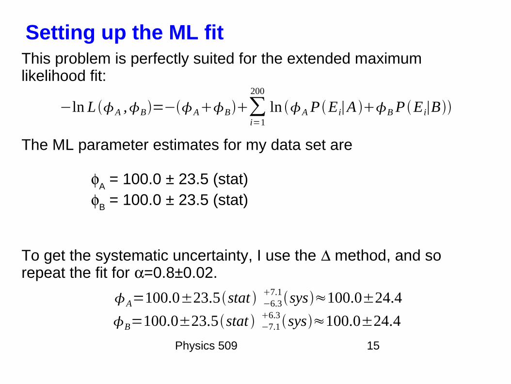
Setting up the ML fitThis problem is perfectly suited for the extended maximum likelihood fit:

The ML parameter estimates for my data set are

A = 100.0 ± 23.5 (stat)

B = 100.0 ± 23.5 (stat)

To get the systematic uncertainty, I use the method, and so repeat the fit for =0.8±0.02.

−ln L A ,B=−AB∑i=1

200

ln AP E i∣A BP E i∣B

A=100.0±23.5stat −6.37.1

sys≈100.0±24.4

B=100.0±23.5stat −7.16.3

sys≈100.0±24.4

Physics 509 16

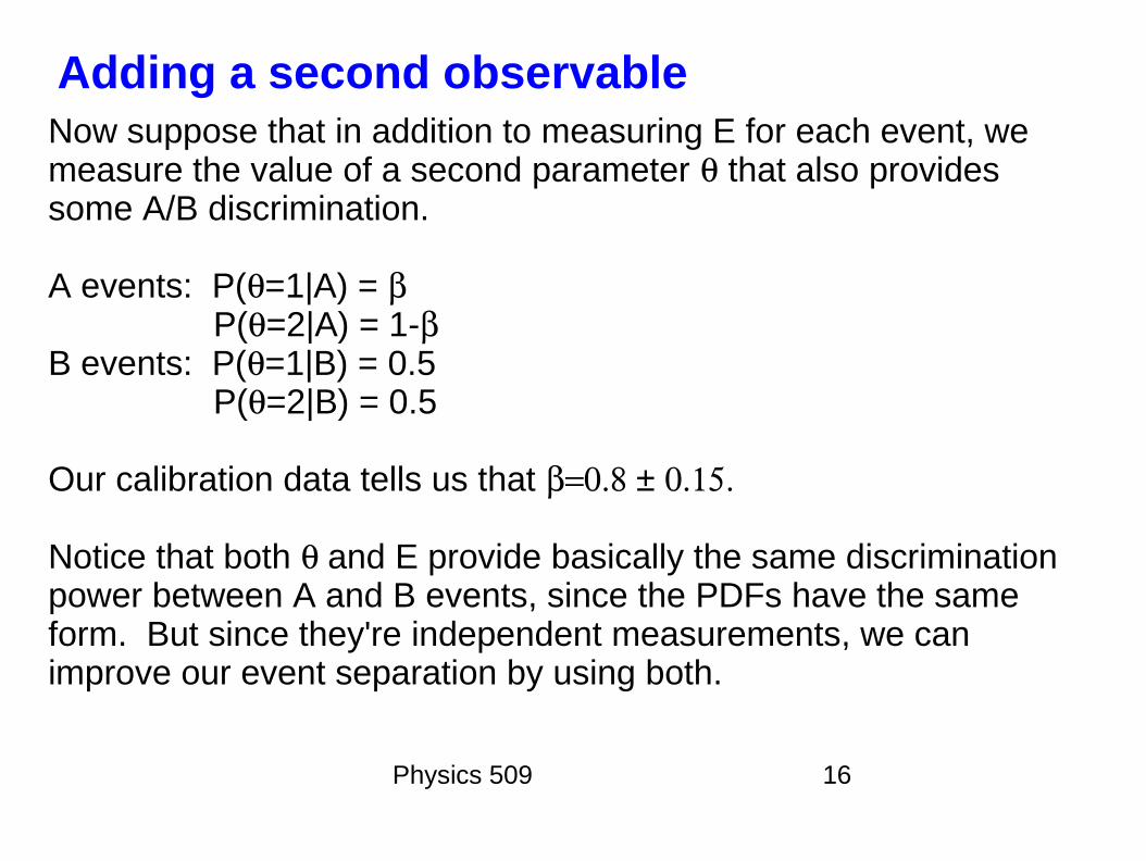
Adding a second observableNow suppose that in addition to measuring E for each event, we measure the value of a second parameter that also provides some A/B discrimination.

A events: P(=1|A) = P(=2|A) = 1-B events: P(=1|B) = 0.5 P(=2|B) = 0.5

Our calibration data tells us that ±

Notice that both and E provide basically the same discrimination power between A and B events, since the PDFs have the same form. But since they're independent measurements, we can improve our event separation by using both.

Physics 509 17

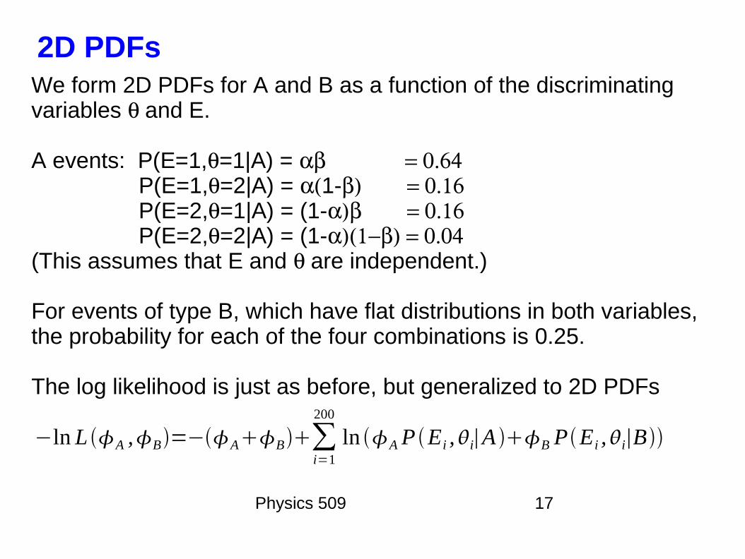
2D PDFsWe form 2D PDFs for A and B as a function of the discriminating variables and E.

A events: P(E=1,=1|A) = P(E=1,=2|A) = 1- P(E=2,=1|A) = (1- P(E=2,=2|A) = (1-(This assumes that E and are independent.)

For events of type B, which have flat distributions in both variables, the probability for each of the four combinations is 0.25.

The log likelihood is just as before, but generalized to 2D PDFs

−ln L A ,B=−AB∑i=1

200

ln AP Ei ,i∣A B PEi ,i∣B

Physics 509 18

Event rates using both E and When I fit the data set using both variables to improve the discrimination, I get:

A = 100.0 ± 18.0 (stat)

B = 100.0 ± 18.0 (stat)

Recall that the statistical error was 23.5 when using just E in the fit. Including the additional information provided further separation between the two classes of events.

(Side note: if I could somehow figure out how to perfectly separate the two kinds of events, the error bars would reduce to √N---this would just become a counting experiment! The fact that the errors are larger than √N reflects the fact that the separation between A and B is imperfect, and in fact the two rate estimates are negatively correlated.)

Physics 509 19

Systematics when using both E and Now I'll propagate the systematics. I have uncertainties on both and . My calibrations of these quantities are independent, so we can safely take them to be independent. Therefore I propagate the systematics using the method with error propagation:

In practice I just vary and separately by their ±1ranges, and add the results in quadrature. My final answer is:

dA2= ∂A

∂ 2

d2 ∂A

∂ 2

d 2

A=100.0±18.0stat −26.717.4

sys ≈100.0−32.225.0

B=100.0±18.0 stat −17.426.7

sys≈100.0−25.032.2

Physics 509 20

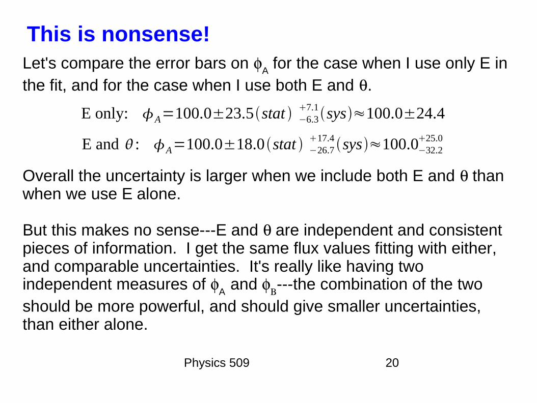
This is nonsense!Let's compare the error bars on

A for the case when I use only E in

the fit, and for the case when I use both E and .

Overall the uncertainty is larger when we include both E and than when we use Ealone.

But this makes no sense---E and are independent and consistent pieces of information. I get the same flux values fitting with either, and comparable uncertainties. It's really like having two independent measures of

A and ---the combination of the two

should be more powerful, and should give smaller uncertainties, than either alone.

E and : A=100.0±18.0 stat −26.717.4 sys≈100.0−32.2

25.0

E only: A=100.0±23.5stat −6.37.1

sys≈100.0±24.4

Physics 509 21

Nonsense revealedThe statistical errors did in fact get smaller when we use both E and . The problem is evidently in the systematic uncertainties.

Imagine that our uncertainty on were infinite---in that case we

have infinite uncertainty on the PDF, and gain no information

from including as a variable in the fit. (Adding infinitely uncertain

information is the same as adding no information at all---the error bar shouldn't increase, it just doesn't get any smaller.)

We have a logical paradox---as long as the uncertainty on is finite, then using as a as a variable in the ML fit should only improve the separation between events of type A and B, and the errors should get smaller.

E and : A=100.0±18.0 stat −26.717.4 sys≈100.0−32.2

25.0

E only: A=100.0±23.5stat −6.37.1

sys≈100.0±24.4

Physics 509 22

What does the “floating systematic” approach yield?The pull method is straightforward to implement:

The hardest part is simply setting up the minimization over 4D and getting it to converge on the minimum, but even that's straightforward.

The best fit result:

A = 100.0 ± 22.7

= 100.0 ± 22.7 = 0.800 ± 0.0197 = 0.800 ± 0.074

−ln LA ,B , , =AB−∑i=1

200

lnAP E i ,i , ,∣A BP E i ,i∣B12 −0.8

0.02 2

12 −0.8

0.15 2

Physics 509 23

Let us contemplate this upon the Tree of Woe ...

CONAN THE BARBARIAN

Physics 509 24

Contemplation of the pull result

The best fit result was:

A = 100.0 ± 22.7

= 100.0 ± 22.7 = 0.800 ± 0.0197 = 0.800 ± 0.074

Note that the overall uncertainty on the rates is smaller than that obtained when fitting only with E (±23.5).

Note as well that the uncertainties on andare smaller than our prior estimates ( = 0.80 ± 0.02 and = 0.80 ± 0.15), especially the estimate on .

The result from the floating systematics fit avoids the mathematical paradox we say in the method of propagating systematics!

Physics 509 25

Why does the pull method work?The pull method puts nuisance parameters on the same footing as other parameters---all are treated as unknowns. The penalty function (“constraint term”) is none other than a frequentist version of the Bayesian prior on the nuisance parameter.

In our example, we had a tight constraint on ±and a weaker constraint on ±. In principle both have equal discriminatory power between A and B events, except for the difference in systematics. Using E, which depends on , gives a good constraint on the rates and These in term can be turned back around to give a tighter constraint on than we had a priori.

In this particular example it was important that the rates depended on both and ---through their effects on the rates they constrain each other. If we had just one or the other, we wouldn't get any benefit from the pull method.

Physics 509 26

Effectively there's a correlation between the nuisance parameters

Even though our prior estimates of and were uncorrelated, the fit procedure itself introduces an effective correlation between the two.(From the fit, cov()=0.144).

The data itself is saying that certain combinations of the two parameters that a priori you would have accepted are not good fits to the data, and should be rejected. For example, if is on the large side, then cannot be too small while still fitting the data. The data effectively prunes the range of reasonable and .

In contrast, the method of propagating systematics gives an incorrect, paradoxical answer.

27

Conclusion: use the pull method!The pull method provides a self-consistent treatment of the data and uncertainties. Other methods do not, and will produce wrong results. You have two choices:

add constraint terms directly to the likelihood, or calculate the covariance matrix between all the data points given the systematic uncertainties, and include that covariance matrix in the likelihood or 2

Generally either approach will give the correct answer, although the first is usually easier, and more obviously yields constraints on the systematics themselves. I recommend that approach.

Do NOT use the method of just varying the systematics one at a time and adding up all of the resulting variations, in quadrature or otherwise. It might work in certain limited circumstances, but in others it is grossly incorrect.

Physics 509

A graphical interpretationConsider a fit for one parameter X with one systematic whose nuisance parameter we'll call c.

The red line represents the 2 for the best fit value of c (including its constraint term).

The blue and purple curves are the 2 vs X curves for two other values of c that don't fit as well. The curves are shifted both up and sideways.

The black curve is the envelope curve that touches the family of 2 curves for all different possible values of c. It is the global 2 curve after marginalizing over c, and its width gives the total uncertainty on X (stat+sys).

Physics 509 29

A simple recipe that usually will work1) Build a quantitative model of how your likelihood function depends on the nuisance parameters.

2) Form a joint negative log likelihood that includes both terms for the data vs. model and for the prior on the nuisance parameter.

3) Treat the joint likelihood as a multidimensional function of both physics parameters and nuisance parameters, treating these equally.

4) Minimize the likelihood with respect to all parameters to get the best-fit.

5) The error matrix for all parameters is given by inverting the matrix of partial derivatives with respect to all parameters:

V=−∂2 ln L∂i∂ j

−1