PH

YS

ICS

LA

B M

AN

UA

L E

NG

INE

ER

ING

SC

IEN

CE

& P

HY

SIC

S D

EP

AR

TM

EN

T

C O L L E G E O F S T A T E N I S L A N D

C I T Y U N I V E R S I T Y O F N E W Y O R K

INS 101 PHYSICS COUNTERPART

THIS MANUAL MUST BE USED ALONG

WITH A DESIGNATED INS LSW PACKET: ASTRONOMY THROUGH PRACTICAL

INVESTIGATIONS.

PACKET MUST INCLUDE: LSW#1 – Measurements & Metric System

LSW#9 – Phases of the Moon LSW#14 – Planetary Configurations

LSW#15 – Constellations LSW#16 – Planetary Properties

One STAR FINDER

INS

101

AST

RO

NO

MY

CO

UN

TE

RPA

RT

"Measure what is measurable, and make measurable what is not so." -- Galileo Galilei

ENGINEERING SCIENCE & PHYSICS DEPARTMENT PHYSICS LABORATORY EXT 2978, 4N-214/4N-215

LABORATORY RULES 1. No eating or drinking in the laboratory premises. 2. The use of cell phones is not permitted.

3. Computers are for experiment use only. No web surfing, reading e-mail, instant

messaging or computer games allowed. 4. When finished using a computer log-off and put your keyboard and mouse away.

5. Arrive on time otherwise equipment on your station will be removed.

6. Bring a scientific calculator for each laboratory session.

7. Have a hard copy of your laboratory report ready to submit before you enter the

laboratory. 8. Some equipment will be required to be signed out and checked back in. The rest

of the equipment should be returned as directed by the technician. Remember, you are responsible for the equipment you use during an experiment.

9. After completing the experiment and, if needed, putting away equipment, check that your station is clean and clutter free.

10. Push in your chair. 11. Before leaving the laboratory premises, make sure that you have all your

belongings with you. The lab is not responsible for any lost items.

Your cooperation in abiding by these rules will be highly appreciated.

Thank You. The Physics Laboratory Staff

INS 101 - Physics Counterpart(For Astronomy experiments refer to LSW packet)

TABLE OF CONTENTS

The laboratory instructor, in order to adjust to the lecture schedule or personal preference, maysubstitute any of the experiments below with supplementary experiments.

1. LABORATORY REPORTS.............................................................................................1

2. MASS AND DENSITY.....................................................................................................5

3. CONSTANT VELOCITY.................................................................................................9

4. MOTION OF A BODY IN FREE FALL.........................................................................12

5. SIMPLE PENDULUM.....................................................................................................16

6. CALORIMETRY.............................................................................................................18

7. OHM’S LAW AND RESISTANCE................................................................................20

8. SOUND WAVES..............................................................................................................22

9. REFLECTION AND REFRACTION...............................................................................25

10. FOCAL POINT AND FOCAL LENGTH OF MIRRORS AND LENSES.....................27

SUPPLEMENTARY EXPERIMENTS:

11. VERNIER CALIPER - MICROMETER CALIPER.........................................................30

12. CENTRIPETAL FORCE.................................................................................................35

13. EQUIPOTENTIALS AND ELECTRIC FIELDS.............................................................37

14. NUCLEAR DECAY........................................................................................................39

15. ATOMIC SPECTRA.......................................................................................................43

APPENDIX:

A1. TABLE OF DENSITIES OF COMMON SUBSTANCES.............................................47

A2. GRAPHICAL ANALYSIS 3.4 - FINDING THE BEST FIT..........................................48

A3. ANALYSIS OF DATA...................................................................................................52

This laboratory manual is the product of the collaboration of faculty members of theEngineering Science & Physics Department.

Diagrams, drawings and tables provided by Jackeline S. Figueroa, Senior CLT, except for:

Page 30: Fig 1, 2 and Page 32: Fig. 4.

LABORATORY REPORTS

The Laboratory Report should contain the following information:

1. Physical Principles: i.e., laws and definitions used.

2. Laboratory Data: arranged in tabular form with labeled rows and columns.

3. Computations and Graphs: See below.

4. Summary of Results: i.e., conclusions and discussion of them, also errors. See below

5. Answers to Questions

I. GRAPHICAL REPRESENTATION OF DATA: Some essentials in plotting a graph.

1. Arrange the numbers to be plotted in tabular form if they are not already so arranged.

2. Decide which of the two quantities is to be plotted along the X-axis and which along the Y-axis. It is customary to plot the independent variable along the X-axis and the dependentalong the Y.

3. Choose the scale of units for each axis of the graph. That is, decide how many squares of the cross-section plotted along a particular axis. In every case the scales of units for the axes must be so chosen that the completed curve will spread over at least one-half of the full-sized sheet of graph paper.

4. Attach a legend to each axis which will indicate what is plotted along that axis and, in

addition, mark the main divisions of each axis in units of the quantity being plotted.

5. Plot each point by indicating its position by a small pencil dot. Then draw a small circlearound the dot so that each plotted point will be clearly visible on the completed graph. Thiscircle is drawn with a radius equal to the estimated probable error of that particularmeasurement (you may use the percent difference when calculable). (See "errors" below).

6. Draw a smooth curve through the plotted points. This curve need not necessarily passthrough any of the points but should have, on the average, as many points on one side of itas it has on the other. The reason for drawing a smooth curve is that it is expected torepresent a mathematical relationship between the quantities plotted. Such a mathematicalrelationship ordinarily will not exhibit any abrupt changes in slope, merely indicates that themeasurement is subject to some error. A close fit of the experimental points to the smoothcurve shows that the measurement is one of small error.

1

7. Label the graph. That is, attach a legend which will indicate, at a glance, what the graph purports to show.

II. ERRORS OF OBSERVATION

1. Blunders: Every measurement is subject to error. Obviously, one should know how to reduceor minimize error as much as possible. The commonest and simplest type of error to removeis a blunder, due to carelessness, in making a measurement. Blunders are diminished byexperience and the repetition of observations.

2. Personal Errors: These are errors peculiar to a particular observer. For example beginnersvery often try to fit measurement to some preconceived notion. Also, the beginner is oftenprejudiced in favor of his first observation.

3. Systematic Errors: Are errors associated with the particular instruments or technique ofmeasurement being used. Suppose we have a book which is 9in. high. We measure itsheight by laying a ruler against it, with one end of the ruler at the top end of the book. If thefirst inch of the ruler has been previously cut off, then the ruler is like to tell us that the bookis 10in. long. This is a systematic error. If a thermometer immersed in boiling pure waterat normal pressure reads 215°F (should be 212°F) it is improperly calibrated; if readingsfrom this thermometer are incorporated into experimental results, a systematic error results.

4. Accidental (or Random) Errors: When measurements are reasonably free from the abovesources of error it is found that whenever an instrument is used to the limit its precision,errors occur which cannot be eliminated completely. Such errors are due to the fact thatconditions are continually varying imperceptibly. These errors are largely unpredictable andunknown. For example: A small error in judgment on the part of the observer, such as inestimating to tenths the smallest scale divisions. Other causes are unpredictable fluctuationsin conditions, such as temperature, illumination, socket voltage or any kind of mechanicalvibrations of the equipment being used. The effect of these errors may be mitigated byrepeating the measurement several times and taking the average of the readings. There are two ways of estimating the error due to random independent measurements. Oneway is to calculate the Mean Absolute Deviation and the other is to calculate the Standarddeviation. Both methods are discussed in the appendix.

5. Significant Figures: Every number expressing the result of a measurement or of computationsbased on measurements should be written with the proper number of "significant figures."The number of significant figures is independent of the position of the decimal point: i.e.8.448cm, 84.48mm, or 0.08448m has the same number of significant figures. A figure ceasedto be a significant when we have no reason to believe, on the basis of measurement made,that the correct result is probably closer to that figure when to the next (higher or lower)figure. In computations, since figures which are not significant in this sense have no placein the final result, they should be dropped to avoid useless labor. e.g. in the measurement ofthe diameter of a penny we read on the ruler 1.748. Here the last figure is a very roughguess; hence, for computations we use 1.75.

2

6. Reading error: Every instrument has a limitation in accuracy. The markings serve as a guideas to that accuracy. We read the instrument to a fraction of the smallest division. As in thediameter of a penny the 8 is an estimated number. We then have to estimate the error in thatnumber. For most applications the reading error can be taken as +/-2. Therefore theexperimental value for that measurement is 1.748 +/- 0.002 cm. The reading error may betaken as a constant error for that instrument. The smallest error associated with ameasurement is the reading error.

7. Percent Error: To present the error in a relative manner we calculate the percent error.

The Measurement error may be estimated from your measurements a variety of ways. Twosimple ways are the standard deviation or the mean absolute error. For most applications themean absolute error is a good estimate of the measurement error.

8. Percent Difference: In your laboratory work you will often find occasion to compare a valuewhich you have obtained as a result of measurement, with the standard, or generally acceptedvalue. The percent difference is computed as follows:

9. If Percent Difference (PD) is smaller than Percent Error (PE), you can conclude that theexperimental value is consistent with the standard (known) value within estimated errors. If,however, PD is larger than PE, the measured value is inconsistent with the standard (known)one. In other words, if PE is estimated correctly, the measured value can be claimed to be abetter estimate of the standard one.

III. The following additional instructions should be complied with.

1. The laboratory report should have a title page giving the name and number of the experiment,the student's name, the class, and the date of the experiment.

2. Each of the five major sections should begin on a new page.

3. Each section should be clearly labeled.

4. Paper should be 8-1/2 x 11 in. Write on one side only using a word processing software.

5. Ruler and compass should be used for diagrams.

6. Reports should be stapled together.

3

7. Please be as neat as possible in order to facilitate reading your report.

8. Reports are due one week following the experiment. No reports will be accepted after the"Due-date" without penalty as determined by the instructor.

9. No student can pass the course unless he or she has turned in a complete set of laboratoryreports.

10. The student is responsible for any further instruction given by his or her teacher.

4

MASS AND DENSITY

Apparatus:

- Electronic balance- Metric ruler- Assorted metallic cylinders- Aluminum bar- Wooden block- Irregular shaped object (mineral/rock sample)- 250ml graduated cylinder

Part I. Mass and Weight:

The mass of a body at rest is an invariable property of that body. It is a measure of the quantity ofmatter in a body. A body has the same mass at the equator as at the North Pole, -- the same masson the earth as on Jupiter or interstellar space.

The gravitational force between the earth (or other planet) and a body is called the weight of the bodywith respect to the earth (or other planet). The gravitational force on a body is a variable quantityeven on the surface of the earth, e.g., the weight of a body is larger at the North Pole than at theEquator. E.g., A book transported to the moon would have the same mass (quantity matter) on themoon as it had back on the earth, but the book weighs less on the moon than it did on the earthbecause the moon's gravitational pull is less than the earth's.

The weight of a body is proportional to its mass, the proportionality factor depending on the placeat which the weight is determined. If the weight of a body is compared with that of a standard body,at the same place on the earth the ratio of the two weights is equal to the ratio of the two masses. Consequently, if the weight of the body is found to be equal to the weight of a standard body at thesame place on earth, the two masses are equal. In order to measure the mass of a body, it isnecessary to find a standard mass or a combination of standard masses whose weight equals that ofa body at the same place on the earth. The device employed for this purpose is called a balance.

Procedure:

1.1. Determine the mass of each object using the balance. Record all data in tabular form.

5

Part II. Volume by measuring dimensions:

Procedure:

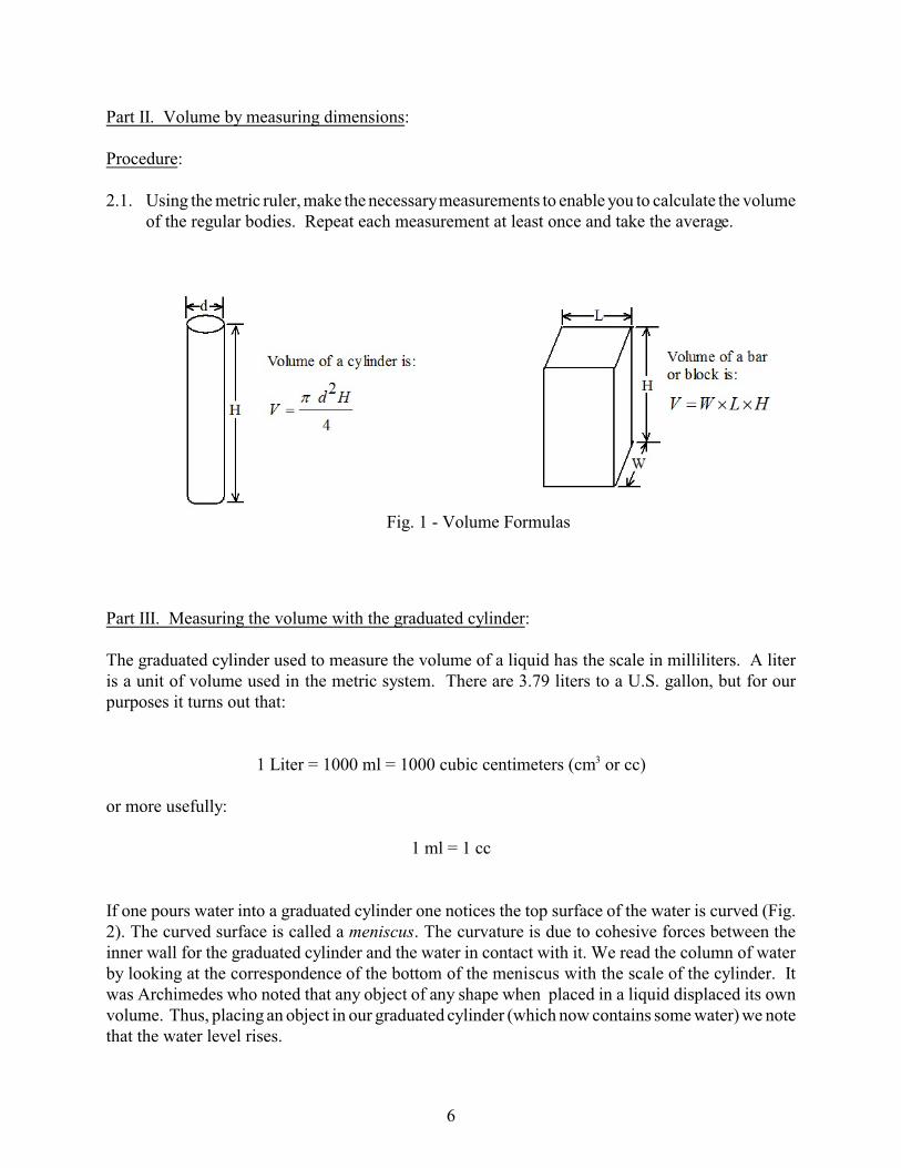
2.1. Using the metric ruler, make the necessary measurements to enable you to calculate the volumeof the regular bodies. Repeat each measurement at least once and take the average.

Part III. Measuring the volume with the graduated cylinder:

The graduated cylinder used to measure the volume of a liquid has the scale in milliliters. A literis a unit of volume used in the metric system. There are 3.79 liters to a U.S. gallon, but for ourpurposes it turns out that:

1 Liter = 1000 ml = 1000 cubic centimeters (cm3 or cc)

or more usefully:

1 ml = 1 cc

If one pours water into a graduated cylinder one notices the top surface of the water is curved (Fig.2). The curved surface is called a meniscus. The curvature is due to cohesive forces between theinner wall for the graduated cylinder and the water in contact with it. We read the column of waterby looking at the correspondence of the bottom of the meniscus with the scale of the cylinder. It was Archimedes who noted that any object of any shape when placed in a liquid displaced its ownvolume. Thus, placing an object in our graduated cylinder (which now contains some water) we notethat the water level rises.

Fig. 1 - Volume Formulas

6

Fig. 2 - Graduated Cylinder

Procedure:

3.1 Use the graduated cylinder to obtain the volume of the objects applicable to this method. Beingenious with the wooden block!

Part IV. Mass Density:

The “mass density” of a material is defined as the mass of any amount of that material divided bythe volume of that amount. The density of a substance is a fixed quantity for fixed externalconditions, and, thus, is a means of identifying a substance. E.g., All different shaped solids ofaluminum have the same density at room temperature. The units of mass density are g/cm3 or kg/m3

in the metric system.

When we use centimeter (cm), grams (g), and seconds (s) in measuring quantities we refer to the cgssystem. Likewise when we use meters (m), kilograms (kg), and seconds (s) we refer to the mkssystem.

Procedure:

4.1. Calculate the mass density of each object in the cgs system.

4.2. Identify the unknown object by using the density you calculated and finding a close match inthe Density Table shown in Appendix A3.

4.3 Calculate the % difference of your density measurements.

Questions:

1. By Archimedes' observation how would you obtain the volume of the object placed in thecylinder?

2. Which value of the volume is closer to the 'truth'? I.e., Part II or III. Explain your answer.

7

3. How do you account for the errors in your computed values of the density(ies)?

4. Which type of measurement done in parts I, II and III do you think you made with the leasterror? i.e., mass or length or volume. Explain.

5. Which of the densities you have just determined would you expect to be the least accurate?

6. What is the benefit, if any, in measuring volumes by using Archimedes’ observations?

8

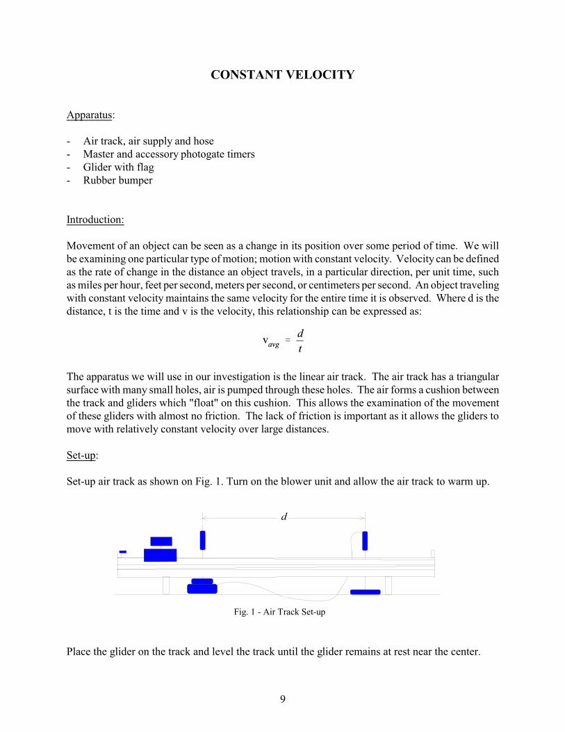
Fig. 1 - Air Track Set-up

CONSTANT VELOCITY

Apparatus:

- Air track, air supply and hose- Master and accessory photogate timers- Glider with flag- Rubber bumper

Introduction:

Movement of an object can be seen as a change in its position over some period of time. We willbe examining one particular type of motion; motion with constant velocity. Velocity can be definedas the rate of change in the distance an object travels, in a particular direction, per unit time, suchas miles per hour, feet per second, meters per second, or centimeters per second. An object travelingwith constant velocity maintains the same velocity for the entire time it is observed. Where d is thedistance, t is the time and v is the velocity, this relationship can be expressed as:

The apparatus we will use in our investigation is the linear air track. The air track has a triangularsurface with many small holes, air is pumped through these holes. The air forms a cushion betweenthe track and gliders which "float" on this cushion. This allows the examination of the movementof these gliders with almost no friction. The lack of friction is important as it allows the gliders tomove with relatively constant velocity over large distances.

Set-up:

Set-up air track as shown on Fig. 1. Turn on the blower unit and allow the air track to warm up.

Place the glider on the track and level the track until the glider remains at rest near the center.

9

Procedure:Set the start and stop gate to give a timing distance of 20cm. With the rubber band set for thesmallest separation, launch the glider and record the time. Be sure not to allow the glider to bounceback and trip the start gate before the time is recorded. Repeat the procedure after moving the stopphotogate to give timing distances of 40cm, 60cm, 80cm and 100cm. Reset the timer each timebefore releasing the glider.

Data Table

d[cm]

t[s]

tavg

[s]v=d/tavg

[cm/s]

20

t1=

t2=

t3=

40

t1=

t2=

t3=

60

t1=

t2=

t3=

80

t1=

t2=

t3=

100

t1=

t2=

t3=

Calculations and Graph:

1. Calculate the average time for each given distance.

2. Use the average time to calculate the average velocity for each position. Compare thesevelocities are they equal? How much do you trust your results?

10

3. Use all the velocities on the 4th column and find the mean.

4. Use the data from the table to plot a graph of d vs. tavg.

5. Determine the slope of the graph, how does it compare to the mean velocity you obtained onCalculation 3?

11

MOTION OF A BODY IN FREE FALL

Apparatus:

S Behr Free-Fall apparatusS Pre-made tape from the free fall apparatusS Meter stick or rulerS Graph paper

Discussion:

In the case of free falling objects the acceleration and the velocity are in the same direction so thatin this experiment we will be able to measure the acceleration by concerning ourselves only withchanges in the speed of the falling bodies. (We recall the definition of acceleration as a change inthe velocity per unit-time and the definition of velocity as the displacement in a specified directionper unit-time.)

A body is said to be in free fall when the only force that acts upon it is gravity. The condition of freefall is difficult to achieve in the laboratory because of the retarding frictional force produced by airresistance; to be more accurate we should perform the experiment in a vacuum. Since, however, theforce exerted by air resistance on a dense, compact object is small compared to the force of gravity,we will neglect it in this experiment.

The force exerted by gravity may be considered to be constant as long as we stay near the surfaceof the earth; i.e., the force acting on a body is independent of the position of the body. The force ofgravity (also known as the weight of the body) is given by the equation:

where m is the mass and g is the acceleration due to gravity

The direction of g is toward the center of the Earth. As shown by Galileo, the acceleration impartedto a body by gravity is independent of the mass of the body so that all bodies fall equally fast (in avacuum). The acceleration is also independent of the shape of the body (again neglecting airresistance).

Useful Information for Constant Acceleration:

12

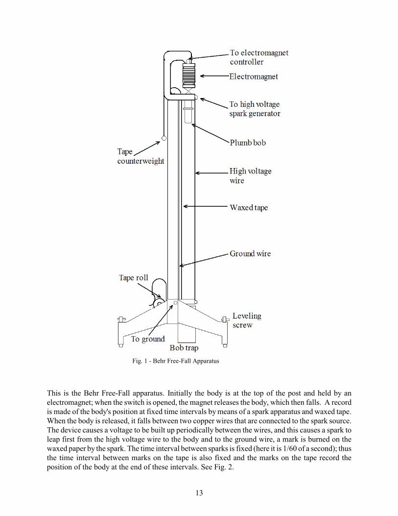
Fig. 1 - Behr Free-Fall Apparatus

This is the Behr Free-Fall apparatus. Initially the body is at the top of the post and held by anelectromagnet; when the switch is opened, the magnet releases the body, which then falls. A recordis made of the body's position at fixed time intervals by means of a spark apparatus and waxed tape. When the body is released, it falls between two copper wires that are connected to the spark source.The device causes a voltage to be built up periodically between the wires, and this causes a spark toleap first from the high voltage wire to the body and to the ground wire, a mark is burned on thewaxed paper by the spark. The time interval between sparks is fixed (here it is 1/60 of a second); thusthe time interval between marks on the tape is also fixed and the marks on the tape record theposition of the body at the end of these intervals. See Fig. 2.

13

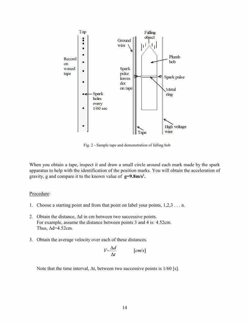
Fig. 2 - Sample tape and demonstration of falling bob

When you obtain a tape, inspect it and draw a small circle around each mark made by the sparkapparatus to help with the identification of the position marks. You will obtain the acceleration ofgravity, g and compare it to the known value of g=9.8m/s2.

Procedure:

1. Choose a starting point and from that point on label your points, 1,2,3 . . . n.

2. Obtain the distance, Äd in cm between two successive points. For example, assume the distance between points 3 and 4 is: 4.52cm. Thus, Äd=4.52cm.

3. Obtain the average velocity over each of these distances.

Note that the time interval, Ät, between two successive points is 1/60 [s].

14

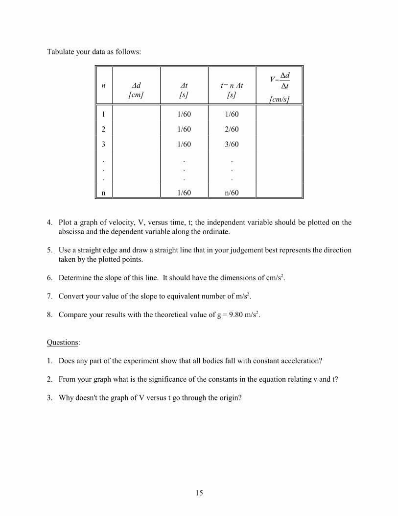
Tabulate your data as follows:

n Äd[cm]

Ät[s]

t= n Ät[s]

[cm/s]

1 1/60 1/60

2 1/60 2/60

3 1/60 3/60

.

.

.

.

.

.

.

.

.

n 1/60 n/60

4. Plot a graph of velocity, V, versus time, t; the independent variable should be plotted on theabscissa and the dependent variable along the ordinate.

5. Use a straight edge and draw a straight line that in your judgement best represents the directiontaken by the plotted points.

6. Determine the slope of this line. It should have the dimensions of cm/s2.

7. Convert your value of the slope to equivalent number of m/s2.

8. Compare your results with the theoretical value of g = 9.80 m/s2.

Questions:

1. Does any part of the experiment show that all bodies fall with constant acceleration?

2. From your graph what is the significance of the constants in the equation relating v and t?

3. Why doesn't the graph of V versus t go through the origin?

15

Fig. 1 - Set-up

Fig. 2 - Simple Pendulum

THE SIMPLE PENDULUM

Apparatus:

S Table clampS Steel rodS Pendulum clamp (silver)S Pendulum bob (various sizes)S StringS Electronic balanceS Master photogate timer (set to pendulum mode)S Meter stickS Pend. Protractor

Introduction:

A simple pendulum consists of a small mass (the pendulum bob) suspended by a non-stretching,

“massless” string of length L. The period T of oscillation is the time for the pendulum bob to gofrom one extreme position to the other and back again.

Consider the variables that determine theperiod of oscillation of a pendulum:

S The amplitude è of oscillation. Theamplitude of the pendulum’s swing is theangle between the pendulum in itsvertical position and either of theextremes of its swings.

S The length L of the pendulum. Thelength is the distance from the point ofthe suspension to the center (of mass) ofthe pendulum bob.

S The mass m of the bob.

S The acceleration due to gravity g.

From unit analysis we can show:

16

Where T = period of oscillation; m = mass of bob; L = length of string; g = acceleration due to gravity

Since an oscillation is described mathematically by cos ùt and knowing that ù=2ðf where

we then have:

Procedure:

Make the following measurements:

1. Set photogate to pendulum mode. Set-up the pendulum so that when it is in resting position itblocks the photogate as shown on Fig. 1.

2. Period as a function of amplitude (plot T vs. è). Use 5o to 60o angles. At a chosen angle allowthe pendulum to swing through the photogate, be careful not to strike the photogate with thependulum. Note: The pendulum only needs to swing 3 times through the photogate to give theperiod.

3. Period as a function of length (plot T 2 vs. L). Use a small amplitude and compare the slope to

4ð2/g

4. Period as a function of mass (plot T vs. m). Use small amplitude.

Questions:

1. For the simple pendulum where is the maximum for: displacement, velocity and acceleration?

2. Would the period increase or decrease if the experiment were held on : a) top of a high mountain?

b) the moon? c) Jupiter?

17

CALORIMETRY

Apparatus:

S CalorimeterS Metal samplesS Glass beaker (600mL)S Hot plateS TongsS Electronic balanceS Plastic beaker S StopwatchS Multimeter (Fluke)

Introduction:

Consider a calorimeter of mass mc and specific heat cc containing a mass of water mw. Suppose thecalorimeter and its contents are initially at some temperature ti. If a hot body of mass ms, specificheat cs, is placed in the calorimeter, then the final equilibrium temperature tf of the entire system canbe measured.

Eq. 1

Eq. 1 assumes no heat losses. From this equation it is possible to determine the temperature th themetal sample had before it was immersed in the calorimeter containing water at room temperature. Therefore,

Eq. 2

Procedure:

1. Fill a glass beaker with water to about 400ml and carefully place it on the hot plate. Turn on thehot plate and set the temperature to approximately 450EC. Let the water heat up while takingother measurements. Keep the calorimeter away from heat source.

2. Measure the mass of the empty inner cup of calorimeter with the stirrer included.

3. Fill the inner vessel with 150ml of cool water. Note that 150ml is equivalent to 150g which isthen represented as mw .

4. Measure the mass of your metal sample.

Fig. 1 - Initial set-up

18

5. Once the water starts to boil carefully place the metal sample in the beaker. Heat the samplefor10 minutes. While the sample is heating note the initial temperature of the calorimeter andits contents just prior to immersing the sample.

6. Immerse the hot sample in the calorimeter and note the final temperature of the system afterequilibrium has been reached.

7. Use Eq. 2 to determine the temperature of the hot metal.

Questions:

1. If the final temperature of the calorimeter and its contents was less than room temperature, wouldthe value of th computed from Eq. 1 be too high or too low? Justify your answer.

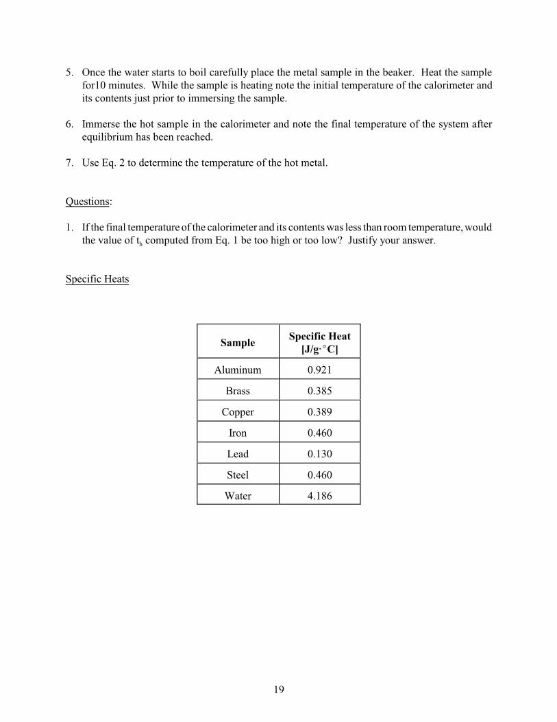
Specific Heats

SampleSpecific Heat

[J/g@EC]

Aluminum 0.921

Brass 0.385

Copper 0.389

Iron 0.460

Lead 0.130

Steel 0.460

Water 4.186

19

OHM’S LAW AND RESISTANCE

Apparatus:

S Variable DC power supplyS 100Ù tubular resistorS Multimeter (I)S 100 watt tungsten filament lampS Lamp socketS SPST switchS Connecting wires

Objective:

To illustrate the voltmeter-ammeter method of measuring resistance and to verify Ohm's Law.

Discussion:

Materials containing electric charges which can move freely are called conductors. Thus, applyingan electric field on such a material results in the mechanical motion of the charges in one particulardirection. This unidirectional motion of electric charges is called electric current.

The applied electric field is characterized by the difference of the electric potential V along theconductor. It is measured in Volts, V. The electric current, I is characterized by the amount ofcharge transferred through the conductor each second. It is measured in Amperes, A.

For most conductors, the relation between V and I follows Ohms’ Law:

Eq. 1

where R is the resistance of the conductor, which does not depend on either V or I. Resistancedepends on various factors -the material the wire is made of, the length of the wire, its cross sectionalarea. Resistance also depends on the temperature of the wire. The unit R is the Ohm, Ù. If graphedon axes V vs I, Eq. 1 yields a straight line whose slope is R.

However, not all conductors obey Ohm’s Law. This means that, if plotted, the data V vs I may befar from that of straight line for such conductors. Such conductors are called non-ohmic.

Procedure:

1. Set up the equipment as shown in Fig 1. Where R is the 100Ù tubular resistor. The flukemultimeter will be used to measure the current I in your circuit. Connect the multimeter in seriesto the resistor with the red connector into the 400mA input and the black connector to the COM input. Set the multimeter to mA and press the yellow key for DC Current. Have yourconnections checked by your instructor before closing the circuit and allowing current to flow.

Fig. 1 - Set-up

20

Vary V in 2V steps from 2V to 30V, recording I and V for each step.

2. Repeat procedure 1, this time using the 100 watt tungsten filament lamp for R. Have yourinstructor check your connections.

Calculations and Graphs:

1. From the data of Procedure 1 plot V as the y-axis and I as the x-axis. If you obtain a straight linethen Ohm’s Law has been verified. Find the slope of the line and compare it to the knownresistance.

2. From the data of Procedure 2 plot V as the y-axis and I as the x-axis. Do you obtain a straightline or a parabolic curve?

Questions:

1. What is the accuracy of your measurements of R in Procedure 1?

2. What is your explanation for the fact that light bulb does not follow Ohm’s Law?

3. From your lamp data and graph find the resistance at 10V.

21

Eq. 1

SOUND WAVES

Apparatus:

S 500ml graduated cylinderS Acrylic tubeS Tuning forks (various frequencies)S Rubber tuning fork activator

Objective:

To determine the wavelengths in air of sound waves of different frequencies by the method ofresonance in closed pipes and to calculate the speed of sound in air using these measurements.

Discussion:

The speed of sound can be measured directly by timing the passage of a sound over a long, knowndistance. To do this with an ordinary watch requires a much longer distance than is available in thelaboratory. It is convenient, therefore, to resort to an indirect way of measuring the speed of soundin air by making use of its wave properties. For all waves the following relationship holds:

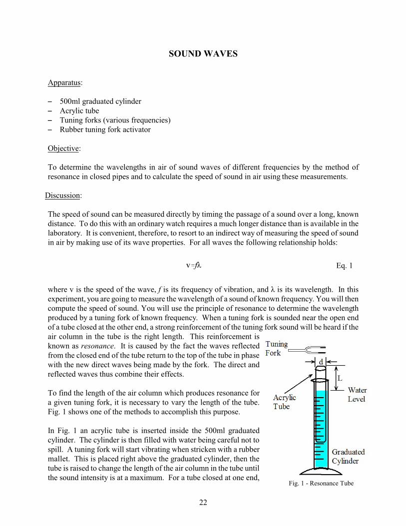
where v is the speed of the wave, f is its frequency of vibration, and ë is its wavelength. In thisexperiment, you are going to measure the wavelength of a sound of known frequency. You will thencompute the speed of sound. You will use the principle of resonance to determine the wavelengthproduced by a tuning fork of known frequency. When a tuning fork is sounded near the open end of a tube closed at the other end, a strong reinforcement of the tuning fork sound will be heard if theair column in the tube is the right length. This reinforcement isknown as resonance. It is caused by the fact the waves reflectedfrom the closed end of the tube return to the top of the tube in phasewith the new direct waves being made by the fork. The direct andreflected waves thus combine their effects.

To find the length of the air column which produces resonance fora given tuning fork, it is necessary to vary the length of the tube. Fig. 1 shows one of the methods to accomplish this purpose.

In Fig. 1 an acrylic tube is inserted inside the 500ml graduatedcylinder. The cylinder is then filled with water being careful not tospill. A tuning fork will start vibrating when stricken with a rubbermallet. This is placed right above the graduated cylinder, then thetube is raised to change the length of the air column in the tube untilthe sound intensity is at a maximum. For a tube closed at one end,

Fig. 1 - Resonance Tube

22

Eq. 2

whose diameter is small compared to its length, strong resonance will occur when the length of theair column is one-quarter of a wavelength, ë/4, of the sound waves made by the tuning fork. A lessintense resonance will also be heard when the tube length is 3/4ë, 5/4ë, and so on.

Since the shortest tube length for which resonance occurs is L=ë/4, it follows that ë. Practically, thisrelationship must be corrected for the diameter d of the tube. This gives:

In this experiment ë, L, and d will be measured in meters.

Procedure:

1. Choose a tuning fork of known frequency. Record the frequency.

2. Insert the resonance tube in the graduated cylinder and start filling it water. Be careful not to spillwater on the desk.

3. Strike the fork on the rubber activator and bring the tuning fork over the open end of thegraduated cylinder. Hold the tuning fork so that the tines vibrate toward and away from thesurface of the water in the cylinder which has the tube inside. Slowly raise the tube until youhear strong resonance. At this point measure the length of the air column in the tube L in metersand record it in your date table.

4. Measure the inner diameter of the hollow tube and record it.

5. Note the room temperature and record it on the table as well.

6. Using several other tuning forks with different frequencies, make the same measurements as inProcedures 1 through 5, except for number 4 which you only need to do once, unless you areusing tubes of different diameter. Record all your measurements on your data table.

Table 1

Frequencyf

[Hz]

Length of AirColumn

L[m]

Diameter ofTube

d[m]

Wavelengthë

[m]

RoomTemperature

T[EC]

Speedv

[m/s]

23

Eq. 3

Calculations:

1. Using the values of L and d in Table 1, calculate the value of the wavelength ë from Eq. 2. Enterthis value of wavelength in the table.

2. Using Eq. 1 calculate the value of the speed of sound in air and record this value in the table foreach of the tuning forks used.

3. Calculate the value of the speed of sound in air from the following relation:

where T is the temperature in degrees centigrade and 331m/s is the speed of sound in air at 0EC.

4. Compare the result obtained by resonance measurement with the calculated value obtained byusing Eq. 3.

Questions:

1. How could you use the method and the results of this experiment to determine whether the speedof sound in air depends upon its frequency? What do your results indicate about such arelationship?

2. If we assume that the speed of sound at any temperature is known from Eq. 3, how can thisexperiment be used to measure the frequency of an unmarked tuning fork?

24

Fig. 1 - Plane Mirror

Fig. 2 - Single ray through a trapezoidal prism

REFLECTION AND REFRACTION

Apparatus:

S Laser ray boxS Trapezoidal acrylic prismS 3-sided mirror (plane, concave and convex)S LED lampS Ruler, protractorS 11x17 paper, masking tape.

Objective:

To investigate Second Law of Reflection and Snell’s Law.

Discussion:

The Second Law of Reflection is basic to the operation of plane and curved mirrors. It will be verified experimentally that the angle of incidence èi is equal to the angle of reflection èr, where èi and èr aremeasured from the normal to the mirror at the point of reflection asin Fig. 1.

èi = èr (Eq. 1)

When dealing with refraction, if a light ray traveling in a medium 1 strikes the surface of a secondmedium 2, in addition to reflection aforementioned, the transmitted ray will be refracted (bent orbroken) changing the direction of its propagation. How much it changes its direction will dependon the optical properties of both mediums called their index of refraction, n. The relationship thatquantifies this dependence is Snell's Law: (Eq. 2)

where è1 is the angle of incidence in themedium n1 and è2 is the angle of refraction inmedium n2. Both angles are measured to thenormal of the surface separating the twomediums as shown in Fig. 2. In the diagrama light ray enters the left side of trapezoidalprism and exits the right parallel side, havingundergone two refractions. Only the firstrefraction has been labeled for è1, è2 and theirNormal NN'.

25

Procedure:

1. Set the plane mirror on a sheet of paper and trace its surface. Set the ray box to produce a singleray and aim the ray toward the center of the mirror so that the ray is reflected back upon itself. Mark the ray with two points spread far enough apart to insure accuracy. Remove the mirror andtrace this ray. This line represents the principal axis of the mirror.

2. Carefully replace the mirror and aim the ray again to strike the mirror at its vertex, but at someangle (say about 30o or so) with the principal axis. Mark both the incident and reflected rays. Theangle between the incident ray and the principal axis is the angle of incidence èi and the anglebetween the reflected ray and the principal axis is the angle of reflection èr . Measure and recordboth angles on your paper. Repeat this procedure for 3 different angles.

3. Draw a straight line and set the trapezoidal prism (frosted side down) vertically in such a way thatthe line goes through the center of the prism as on Fig. 2 line N-N’. Trace the outline of thetrapezoid. Set the ray box to produce a single ray, set it so that the ray passes through the twoparallel faces of the trapezoid. Note that the incident ray should enter the trapezoid at the samepoint where the Normal line, N, meets the first surface of the prism. Carefully mark the incidentand emergent rays. Remove the trapezoid and construct the incident and emergent rays, andconnect them with a straight line representing the internal ray as in Fig. 2. Measure and recordthe angles of incidence è1 and angle of refraction è2.

Calculations:

1. From the results of procedure 2, compare èi and èr for the plane mirror.

2. From the results of Procedure 3, calculate the index of refraction, n2, of the prism (secondmedium) and compare to the known index for acrylic (plexi-glass). Note that the index ofrefraction for the first medium, air, is n1 = 1.00.

CWC

26

Fig. 1 - Focal points for concave and convex mirrors

FOCAL POINT AND FOCAL LENGTH OF MIRRORS AND LENSES

Apparatus:

S Laser ray boxS 3-sided mirror (plane, concave and convex)S Diverging and converging lensesS LED lampS RulerS 11x17 paper, masking tape.

Objective:

To find the focal point and focal length of mirrors and lenses.

Discussion:

Based solely on their refracting properties and shapes, lenses are capable of forming images ofobjects placed in front of them. Mirrors based their capacity to achieve this on their reflectingproperties and shapes. Both lenses and mirrors focus light and have well defined focal points F andfocal lengths ƒ. This same, single property generates both of their abilities. We should not besurprised that our treatment, here for lenses, will be strongly similar.When parallel rays of light or light from infinitely distant objects fall on a mirror, the image point,real as in Fig. 1(a) or virtual as in Fig. 1(b), is called the focal point, F of the mirror. The focallength, ƒ is the distance between F and the mirror. These distances are always measured along theso called principal or optic axes of the mirrors, which is the perpendicular bisector of the mirror.Note that the focal points for the rays in Fig. 1(a) and (b) are on this principal axis. The point wherethe principal axis intersects the mirror is called the vertex of the mirror.

27

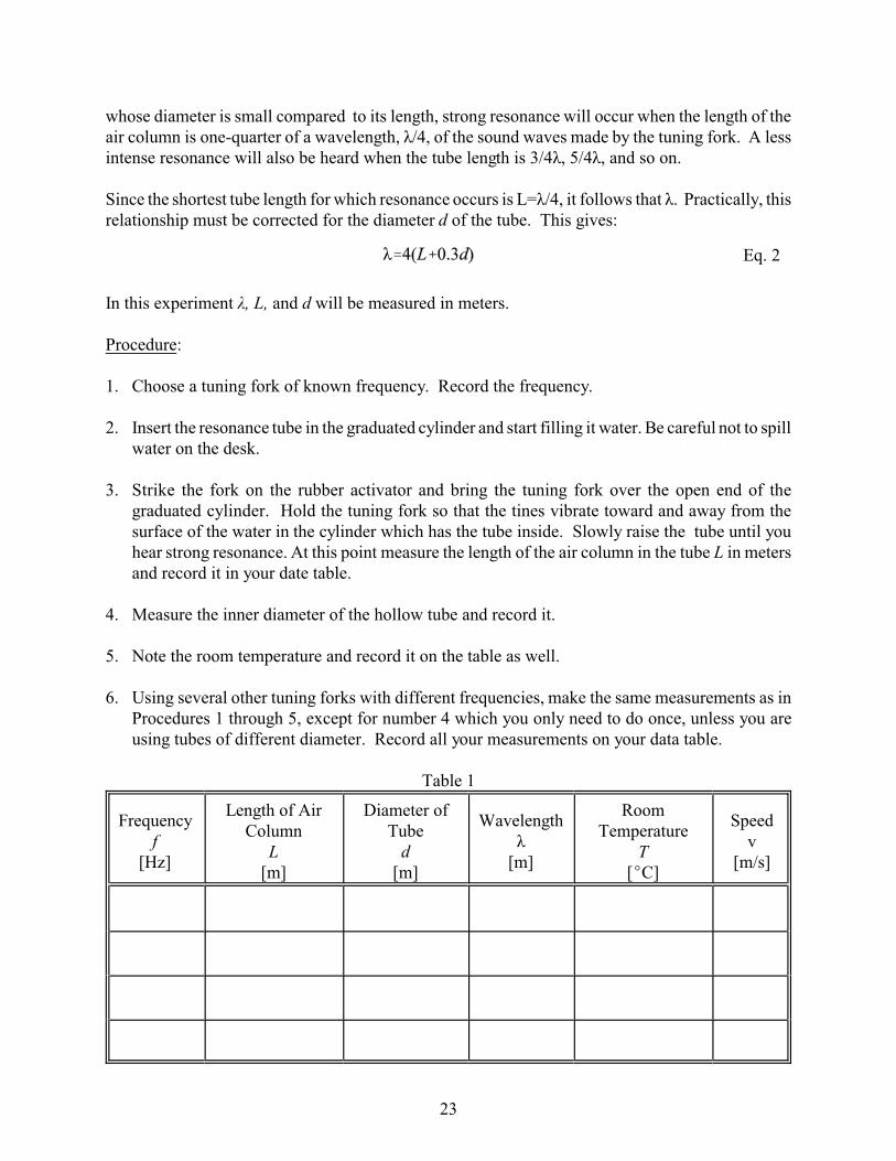
Fig. 2 - Converging and Diverging Lenses

As with mirrors, there are two distinctly different types of lenses that can be identified. They arecorrectly referred to as converging and diverging lenses, not convex and concave. Each lens has twofocal points, which are determined by passing a parallel beam of light through a lens, as shown onFig. 2.

Procedure:

1. Locate and draw the principal axis of your concave mirror. Trace the mirror. Set the ray box to produce a bundle of parallel rays. Aim the rays at the mirror, parallel to its optic axis, so that thereflected rays cross each other back on the axis. Label this point F.Measure the distance of F the mirror in centimeters. This distance is the focal length, ƒ.

2. Repeat this procedure using the convex mirror. Here the reflected ray will have to be extendedback behind the mirror to the principal axis. Since F is now behind the mirror, the focal lengthƒ is negative.

3. On a new page, draw a line along its length, near the middle of the page. This line will representthe principal axis for your lens. Place the center of the converging lens at the middle of the axisand perpendicular to it. Trace the lens on the paper. Be careful not to let the lens move off ofits trace, throughout the procedure.Set the ray box to produce a bundle of parallel rays. Locate and mark the first focal point F bydirecting these rays along the optic axis and marking their point of convergence. Measure andrecord the focal length ƒ.

4. Repeat Procedure 3, using the diverging lens. Note that this time the focal point will be behindthe lens. Refer to Fig. 2b.

CWC

28

SUPPLEMENTARYEXPERIMENTS

29

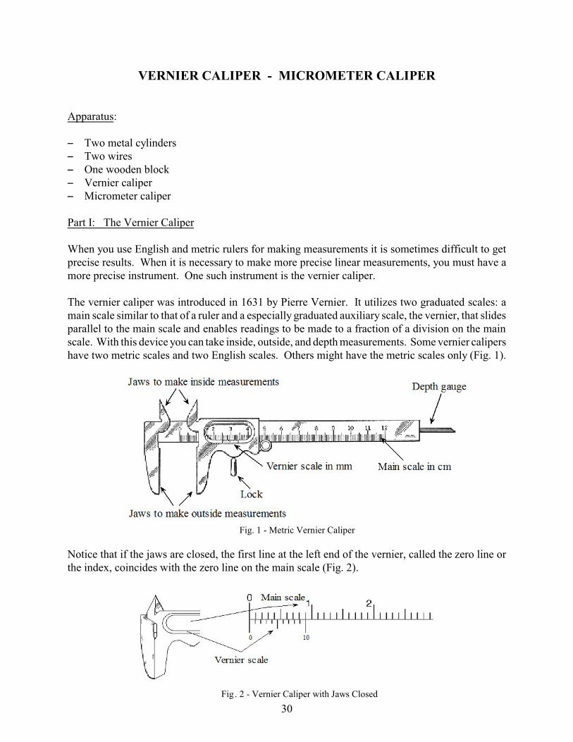
Fig . 2 - Vernier Caliper with Jaws Closed

Fig. 1 - Metric Vernier Caliper

VERNIER CALIPER - MICROMETER CALIPER

Apparatus:

S Two metal cylindersS Two wiresS One wooden blockS Vernier caliperS Micrometer caliper

Part I: The Vernier Caliper

When you use English and metric rulers for making measurements it is sometimes difficult to getprecise results. When it is necessary to make more precise linear measurements, you must have amore precise instrument. One such instrument is the vernier caliper.

The vernier caliper was introduced in 1631 by Pierre Vernier. It utilizes two graduated scales: amain scale similar to that of a ruler and a especially graduated auxiliary scale, the vernier, that slidesparallel to the main scale and enables readings to be made to a fraction of a division on the mainscale. With this device you can take inside, outside, and depth measurements. Some vernier calipershave two metric scales and two English scales. Others might have the metric scales only (Fig. 1).

Notice that if the jaws are closed, the first line at the left end of the vernier, called the zero line orthe index, coincides with the zero line on the main scale (Fig. 2).

30

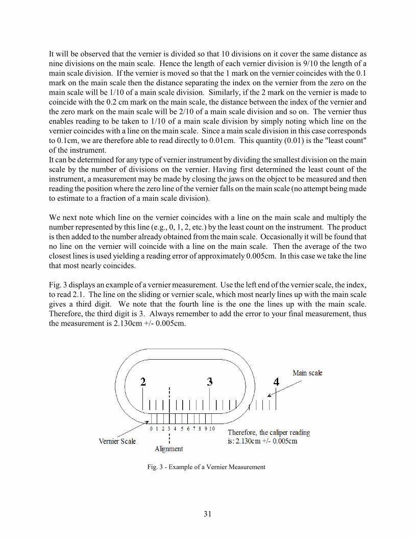
Fig. 3 - Example of a Vernier Measurement

It will be observed that the vernier is divided so that 10 divisions on it cover the same distance asnine divisions on the main scale. Hence the length of each vernier division is 9/10 the length of amain scale division. If the vernier is moved so that the 1 mark on the vernier coincides with the 0.1mark on the main scale then the distance separating the index on the vernier from the zero on themain scale will be 1/10 of a main scale division. Similarly, if the 2 mark on the vernier is made tocoincide with the 0.2 cm mark on the main scale, the distance between the index of the vernier andthe zero mark on the main scale will be 2/10 of a main scale division and so on. The vernier thusenables reading to be taken to 1/10 of a main scale division by simply noting which line on thevernier coincides with a line on the main scale. Since a main scale division in this case correspondsto 0.1cm, we are therefore able to read directly to 0.01cm. This quantity (0.01) is the "least count"of the instrument. It can be determined for any type of vernier instrument by dividing the smallest division on the mainscale by the number of divisions on the vernier. Having first determined the least count of theinstrument, a measurement may be made by closing the jaws on the object to be measured and thenreading the position where the zero line of the vernier falls on the main scale (no attempt being madeto estimate to a fraction of a main scale division).

We next note which line on the vernier coincides with a line on the main scale and multiply thenumber represented by this line (e.g., 0, 1, 2, etc.) by the least count on the instrument. The productis then added to the number already obtained from the main scale. Occasionally it will be found thatno line on the vernier will coincide with a line on the main scale. Then the average of the twoclosest lines is used yielding a reading error of approximately 0.005cm. In this case we take the linethat most nearly coincides.

Fig. 3 displays an example of a vernier measurement. Use the left end of the vernier scale, the index,to read 2.1. The line on the sliding or vernier scale, which most nearly lines up with the main scale gives a third digit. We note that the fourth line is the one the lines up with the main scale. Therefore, the third digit is 3. Always remember to add the error to your final measurement, thusthe measurement is 2.130cm +/- 0.005cm.

31

Fig. 4 - Micrometer Caliper

Procedure:

1. Make two independent measurements of each dimension of the wooden block.

2. Make two measurements of the length and of the diameter of each metal cylinder and each wire.

Questions:

1. Why did you take two independent measurements for each dimension above?

2. What does the smallest division on the main scale of the vernier caliper correspond to?

3. Inspect the vernier scale and note that 10 vernier divisions correspond to 9 main scale divisions. Prove that the vernier can be used to make readings to 1/10 of a main scale division.

Part II. The Micrometer Caliper:

The micrometer caliper, invented by William Gascoigne in the 17th century, is typically used tomeasure very small thicknesses and diameters of wires and spheres. It consists of a screw of pitch0.5mm, a main scale and another scale engraved around a thimble which rotates with the screw andmoves along the scale on the barrel. The barrel scale is divided into millimeters, on someinstruments, such as ours, a supplementary scale shows half millimeters.

32

Fig. 5 - Sample Reading on Micrometer

The thimble scale has 50 divisions. Since one complete turn of the thimble will produce an axialmovement of 0.5mm. One scale division movement of the thimble past the axial line of the scale onthe barrel is equivalent to 1/100 times 1.0 equals 0.01mm. Hence readings may be taken directly toone hundredth of a millimeter and by estimation (of tenths of a thimble scale division) to athousandth of a millimeter.

The object to be measured is inserted between the end of the screw (the spindle) and the anvil on theother leg of the frame. The thimble is then rotated until the object is gripped gently. A ratchet at theend of the thimble serves to close the screw on the object with a light and constant force. Thebeginner should always use the ratchet when making a measurement in order to avoid too great aforce and possible damage to the instrument.

The measurement is made by noting the position of the edge of the thimble on the barrel scale andthe position of the axial line of the barrel on the thimble scale and adding the two readings. Themicrometer should always be checked for a zero error. This is done by rotating the screw until itcomes in contact with the anvil (use the ratchet) and then noting whether the reading on the thimblescale is exactly zero. If it is not, then this "zero error" must be allowed for in all readings.

To read a measurement, simply add the number of half-millimeters to the number of hundredths ofmillimeters. In the example below, we have 2.620mm+/-0.005mm, that is 5 half millimeters and 12hundredths of a millimeter.

If two adjacent tick marks on the moving barrel look equally aligned with the reading line on thefixed barrel, then the reading is half way between the two marks. In the example above, if the 12th

and 13th tick marks on the moving barrel looked to be equally aligned, then the reading would be2.625mm+/-0.005mm.

Procedure:

1. Repeat all measurements that are possible of part I using the micrometer.

2 Measure the diameter of a human hair.

33

Questions:

1. Would you use the vernier to measure the diameter of a human hair? Why?

2. What does one division on the barrel of the caliper correspond to?

3. What does one division on the rotating thimble correspond to?

4. Define metric scale.

5. What does “pitch 0.5 mm” mean?

6. What type (name) of error is the "zero error" of the micrometer assuming it enters a calculation?

34

Fig. 1 - Centripetal Force Apparatus and Display of Static Test

Eq. 1

CENTRIPETAL FORCE Apparatus:

S Centripetal force apparatusS Set of slotted weightsS 50g hangerS StopwatchS Electronic balanceS Level S Ruler

Theory:

A mass m moving with constant speed v in a circular path of radius r must have acting on it acentripetal force F where n is the revolutions per sec.

Description:

As indicated in Fig. 1, the shaft, crossarm, counterweight, bob, and spring are rotated as a unit. Theshaft is rotated manually by twirling it repeatedly between your finger at its lower end, where it isknurled. With a little practice it is possible to maintain the distance r essentially constant, asevidenced for each revolution by the point of the bob passing directly over the indicator rod. Thecentripetal force is provided by the spring.

The indicator rod is positioned in the following manner: with the bob at rest with the springremoved, and with the crossarm in the appropriate direction, the indicator rod is positioned andclamped by means of thumbscrews such that the point of the bob is directly above it, leaving a gapof approximately 2 to 3mm.

The force exerted by the (stretched) spring on the bob when the bob is in its proper orbit isdetermined by a static test, as indicated in Fig. 1 (Static Test).The mass m in Eq. 1 is the mass of the bob. A 100gm slotted mass may be clamped atop the bobto increase its mass.The entire apparatus should be leveled so that the shaft is vertical.

35

Procedure:

Devise a method for determining whether the shaft is vertical, and make any necessary adjustmentsof the three leveling screws.

The detailed procedure for checking Eq. 1experimentally will be left to the student. Atleast three values of r should be used, withtwo values of m for each r. A method formeasuring r should be thought out, for whichpurpose the vernier caliper may be useful. The value of n should be determined bytiming 50 revolutions of the bob, and thenrepeating the timing for an additional 50revolutions. If the times for 50 revolutionsdisagree by more than one-half second,either a blunder in counting revolutions hasbeen made, or the point of the bob has notbeen maintained consistently in its propercircular path.

Results and Questions:

1. Exactly from where to where is r measured? Describe how you measured r.

2. Tabulate your experimental results. 3. Tabulate your calculated results for n, F from static tests, and F from Eq. 1, and the % difference

between the F's, using the static F as standard.

4. Describe how to test whether the shaft is vertical without the use of a level. Why should it beexactly vertical?

5. Why is the mass of the spring not included in m?

6. Discuss your results, and point out sources of error.

36

Eq. 1

EQUIPOTENTIAL LINES AND ELECTRIC FIELDS

Apparatus:

S Conductive PaperS Adhesive copper dots and stripsS Cork boardS Metal push pinsS White paper (8½"x14")S Carbon paperS Digital multimeter with probesS Connecting wires with alligator clipsS 4 x D-size battery holder

Objective:

To measure and plot the equipotentials of various charge configurations and use them to determineand study the Electric Fields that these charge distributions produce.

Discussion:

If a charged particle is placed at a certain point in space and experiences a force, then an electric fieldis said to exist at that point. The strength of the field is given by the electric intensity, a vectorquantity whose magnitude is the force per unit charge and whose direction is the direction of theforce on a small positive test charge qo. That is:

where is the electric intensity. The family of curves, whose tangents point in the direction of the

electric intensity, are known as lines of electric force.

The difference of potential, Vab between two points a and b in an electric field is defined as the workper unit charge required to move a positive test charge from point a to point b. The absolutepotential Va at a point a is usually defined as the work per unit charge required to move a positivetest charge from infinity to the point a. The locus of all points at the same potential is known as theequipotential surface.

Procedure:

1. Set up the experiment for Two Point Charge configuration, as in Fig. 2a.

Fig. 1 - Experiment Set-Up

37

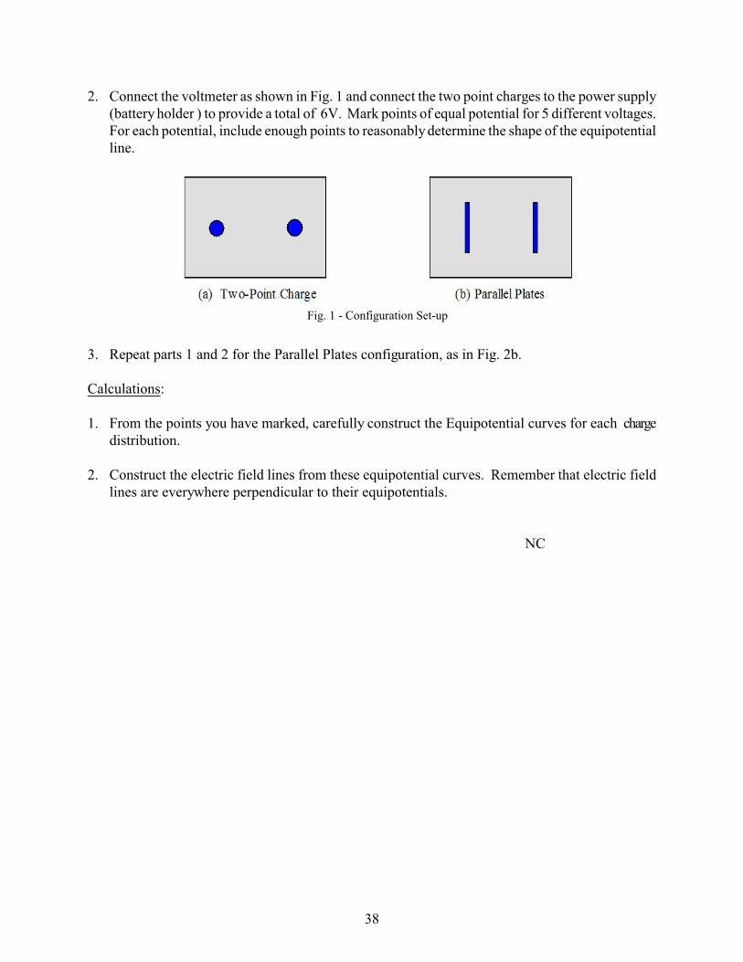
Fig. 1 - Configuration Set-up

2. Connect the voltmeter as shown in Fig. 1 and connect the two point charges to the power supply(battery holder ) to provide a total of 6V. Mark points of equal potential for 5 different voltages.For each potential, include enough points to reasonably determine the shape of the equipotentialline.

3. Repeat parts 1 and 2 for the Parallel Plates configuration, as in Fig. 2b.

Calculations:

1. From the points you have marked, carefully construct the Equipotential curves for each chargedistribution.

2. Construct the electric field lines from these equipotential curves. Remember that electric fieldlines are everywhere perpendicular to their equipotentials.

NC

38

NUCLEAR DECAY SIMULATION

Apparatus:

S 60 diceS Large plastic basin (to hold and toss them)S 2000ml plastic beaker Objective:To explore the radioactive decay behavior and make predictions to its outcome for a group of atoms.

Introduction:You will be given 60 dice representing 60 radioactive parent nuclei. When a parentdecays(transforms into another nucleus) we say the resulting atom is the daughter nuclei. Each throwof the dice represents for our simulation one cycle of time (a millionth of a second, a year, a thousandyears or million or billion). We will assume that any of the dice that show a "6" is one that hasdecayed. We remove all "sixes" and count the remaining atoms whose number we will put in thedata table below. We throw the remaining atoms and remove the next set of sixes. We tabulate aftereach throw the number remaining. Can we predict this number?

This process sets up a simulation of our atoms changing into another. Since real atoms each have achance or probability of decaying (rather than being predictable) our simulation tries to mimic thereal world, in this case, by being a statistical or probabilistic prediction.

In this simulation we assume if a die has a "6" up it indicates that it has decayed. The probability ofdecay for each die is 1/6. i.e. one out of six sides of the die or if we had 6 dice after one throw wewould have one decay. If the probability for 1 die is 1/6 that it will decay then the probability it willnot decay is 5/6 for the first throw. The second throw (or time period) is independent of the first,therefore, by probability theory, the probability a die will not decay is (5/6)2 . For the third timeperiod we get (5/6)3 and so forth. Overall, for 60 dice the number that should survive is 60 times theprobability of survival of one. We can thus generate the formula for the number of radioactive nucleileft, N, is

N = 60 x(5/6)t Eq. 1for time period t. The resulting Probability Curve values are listed in the DATA TABLE BELOW. For example, afterthe fourth time interval we should have left 60 x(5/6)four =60 x .4823 = 28.94 which you see enteredin the data table in the 4th throw number(time period) and Probability law column.

The DECAY CURVE used in your text is called an exponential curve and is theoretically shown toresult from eEq. 1 as the number of time intervals approach infinity. The resulting exponential decaycurve law (the curve is shown in your textbook) gives rise in this case for the number of radioactivenuclei left, N, is

N = 60 e-t/6 Eq. 2 for time period t.

39

You can find the exponential function "e" on a scientific calculator and, for example, after the forthtime interval we should have left by this exponential law 60 x e-4/6 = 60 x .5134 = 30.80 which yousee entered in the data table in the 4th. throw number (time period) and Exponential Law column.In the two examples presented we see that the numbers 28.94 and 30.80 are close for the predictionof how many atoms are left. In fact, figure 1 shows a plot of each law for 12 time periods (12 throwof the dice). It is not difficult to see that both laws match each other closely. In fact, as the numberof time intervals increases the probabilistic curve (plotted square points) approaches the exponentialone (the plotted plus points).

Fig. 1 demonstrates how the exponential equation (Eq. 2) results from the probabilistic equation(Eq.1) as the number of time intervals increases. This is actually how the original exponential curveof decay was derived in 1905.

Procedure:

1. Throw the 60 dice for the first cycle of trial I and remove all the decayed atoms(the "6" 's) andenter the number left for the first time interval (throw number 1) in the data table below.

Fig. 1- Exponential and Probability Curves

40

NUCLEAR SIMULATION DATA TABLE

ThrowNo.

Undecayed Atoms (Dice) - 3Different Trials Avg.

I6 III Prob.Law

Exp.Law

I II III

0 60 60 60 60 60.00 60.00

1 50.00 50.79

2 41.67 42.99

3 34.72 36.39

4 28.94 30.80

5 24.11 26.08

6 20.09 22.08

7 16.74 18.69

8 13.95 15.82

9 11.63 13.39

10 9.69 11.33

11 8.08 19.59

12 6.73 8.12

13 5.61 6.88

14 4.67 5.82

15 3.89 4.93

Half life time for 30 left 3.82 4.17

Half life time for 15 left 3.81 4.17

Half life time for 7.5 left 3.81 4.17

Average of the three half-life times 3.81 4.17

% Diff. of avg. half life from exponential (4.17)

% Diff. of avg. half life from probability (3.81)

Continue for the rest of the fifteen throws for trial number I each time taking out the "6" 's and recording how many are left. Use the Nuclear Simulation Data Table to record your data.

41

2. Repeat procedure 1 for trials II and III and fill in the table for all fifteen time intervals and III trials.

3. Compute the average of each row and enter into the average column. Plot on graph paper allaverage values for throw 0 to 15. as well as the probability law values and Exponential lawvalues.

4. Which of the theoretical curves does your data match? Why?

5. Estimate the half-life times from your graph by figuring out how much time must pass to go from60 to 30, 30 to 15 and 15 to 7.5 and enter these values in the data table.(If you can interpolatethen do so!)

6. Average the three half-lives and enter into the table.

7. Compute the % diff from the exponential result shown in the table and enter it into the table usingthe formula

% diff from Exp.

8. Compute the % diff from the probabilistic result shown in the table and enter it into the tableusing the formula

% diff from Prob.

9. Which %diff result is less? Why?

42

Eq. 1

ATOMIC SPECTRA

Apparatus:

- Meter stick- Diffraction grating (600 lines/mm)- Grating holder- Scale with a slit- Meter stick supports- Spectrum tube power supply- Spectrum tube (He, H2)

Objective:

To use the effect of light interference to measure the wavelengths of light emitted by various atoms.

Theory:

Every chemical element or compound, upon being (by delivering energy to it), emits a unique pattern of wavelengths of light (or colors, each color corresponds to a particular wavelength of the lightwave). In fact, such a pattern makes it possible to recognize unambiguously the element presenceeven in a very tiny amount. Therefore, to analyze the pattern precisely, the wavelengths of lightshould be measured. This direct measurement would be difficult to perform because of very smallvalues of visible light (400-700nm). However, the exploitation of the wave properties— interference and diffraction— turns out to be very helpful.

The interference effect has already been used to measure the wavelength of a sound wave (see theexperiment on Sound Waves). In fact, standing waves can also be formed by light similarly to whathappened with sound in the resonating pipe. In this experiment, another device— the diffractiongrating— will be used to explore the interference of light. A key element of the grating are the verytiny parallel lines set on the transparent slide. The distance d between these lines is a very importantparameter. Normally, each grating is labeled as to how many line per mm it has, from which thedistance d can be determined.

Light striking the grating splits into many rays which, then interfere with each other. As a result, theinterference antinodes (bright lines) are formed on the screen. The position of each antinodedepends on the wavelength ë and the parameter d. This dependence is given by the followingequation:

Where a is the angle of diffraction (Fig. 2) and n=0,1,2,3 stands for the order of the antinode.

43

Eq. 2

Fig. 2 - Diffraction and interference of light due to the diffraction grating

Eq. 3

Eq. 4

Measuring S, the distance from the grating to the screen, and x, the distance from the zero orderantinode to the n-th order antinode, the angle a can be found as:

From Eq. 1 the wavelength can then be determined as

Substituting the sin(a) from Eq. 2, we arrive at:

You will use Eq. 4 to determine the wavelengths corresponding to the colored lines you will observein the spectrum of each tube under study.

Procedure:

Note: Each chemical element is excited by a HIGH VOLTAGE ELECTRIC DISCHARGEwhich is dangerous if handled improperly. Never touch the spectrum tube or its holders.(SHOCK HAZARD!)

1. Set up the equipment as shown in Fig. 1.

2. The human eye will play the role of the screen in this experiment. The scale with the slit is to beaimed at the spectrum tube containing the glowing element.

44

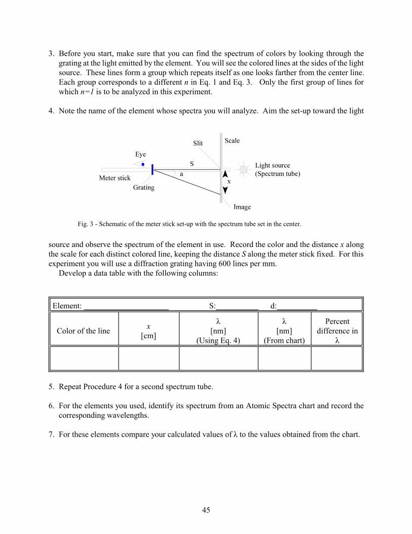
Fig. 3 - Schematic of the meter stick set-up with the spectrum tube set in the center.

3. Before you start, make sure that you can find the spectrum of colors by looking through the grating at the light emitted by the element. You will see the colored lines at the sides of the lightsource. These lines form a group which repeats itself as one looks farther from the center line. Each group corresponds to a different n in Eq. 1 and Eq. 3. Only the first group of lines forwhich n=1 is to be analyzed in this experiment.

4. Note the name of the element whose spectra you will analyze. Aim the set-up toward the light

source and observe the spectrum of the element in use. Record the color and the distance x alongthe scale for each distinct colored line, keeping the distance S along the meter stick fixed. For thisexperiment you will use a diffraction grating having 600 lines per mm.

Develop a data table with the following columns:

Element: S: d:

Color of the linex

[cm]

ë[nm]

(Using Eq. 4)

ë[nm]

(From chart)

Percentdifference in

ë

5. Repeat Procedure 4 for a second spectrum tube.

6. For the elements you used, identify its spectrum from an Atomic Spectra chart and record the corresponding wavelengths.

7. For these elements compare your calculated values of ë to the values obtained from the chart.

45

APPENDIX

46

A1. TABLE OF DENSITIES OF COMMON SUBSTANCES*

Name Density[g/cm3]

NameDensity[g/cm3]

NameDensity[g/cm3]

NameDensity[g/cm3]

Aluminum 2.70 Calcite 2.72 Ash 0.56 Cement 1.85

Brass 8.44 Diamond 3.52 Balsa 0.17 Chalk 1.90

Copper 8.95 Feldspar 2.57 Cedar, red 0.34 Clay 1.80

Iron 7.86 Halite 2.12 Corkwood 0.21 Cork 0.24

Lead 11.48 Magnetite 5.18 Douglas Fir 0.45 Glass 2.60

Nickel 8.80 Olivine 3.32 Ebony 0.98 Ice 0.92

Silver 10.49 Mahogany 0.54 Sugar 1.59

Tin 7.10 Oak, red 0.66 Talc 2.75

Zinc 6.92 Pine, white 0.38

*See the “American Institute of Physics Handbook” for a more extensive list. All values in cgs(g/cc) and at 20E C.

47

A2. GRAPHICAL ANALYSIS 3.4*(Adapted from Venier GA Help Menu)

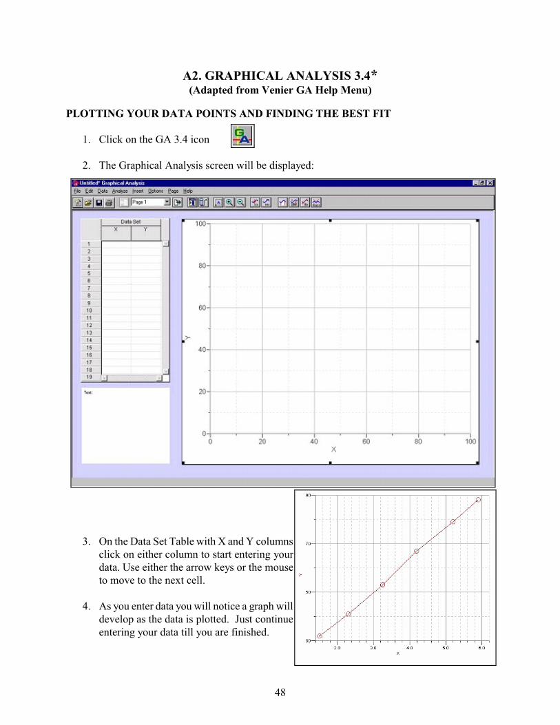
PLOTTING YOUR DATA POINTS AND FINDING THE BEST FIT

1. Click on the GA 3.4 icon

2. The Graphical Analysis screen will be displayed:

3. On the Data Set Table with X and Y columnsclick on either column to start entering yourdata. Use either the arrow keys or the mouseto move to the next cell.

4. As you enter data you will notice a graph willdevelop as the data is plotted. Just continueentering your data till you are finished.

48

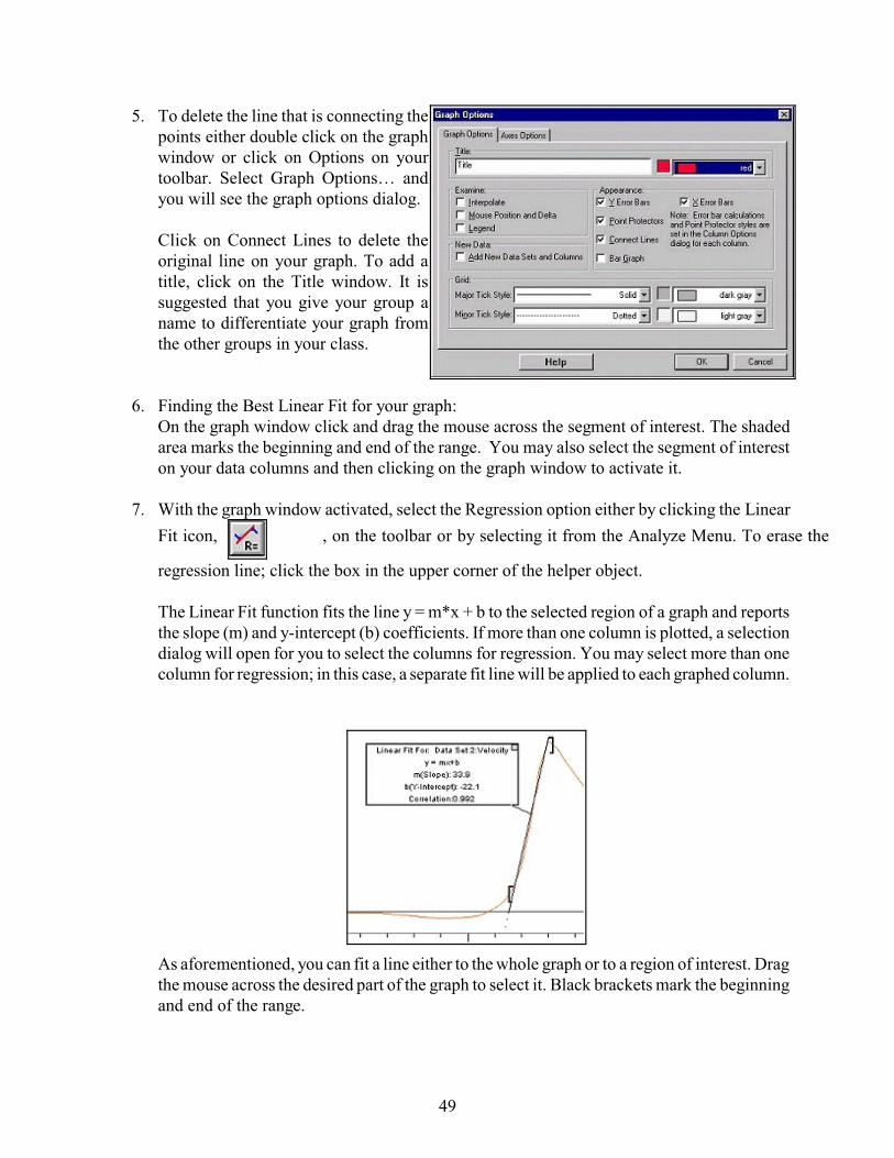
5. To delete the line that is connecting thepoints either double click on the graphwindow or click on Options on yourtoolbar. Select Graph Options… andyou will see the graph options dialog.

Click on Connect Lines to delete theoriginal line on your graph. To add atitle, click on the Title window. It issuggested that you give your group aname to differentiate your graph fromthe other groups in your class.

6. Finding the Best Linear Fit for your graph:On the graph window click and drag the mouse across the segment of interest. The shadedarea marks the beginning and end of the range. You may also select the segment of intereston your data columns and then clicking on the graph window to activate it.

7. With the graph window activated, select the Regression option either by clicking the Linear

Fit icon, , on the toolbar or by selecting it from the Analyze Menu. To erase the

regression line; click the box in the upper corner of the helper object.

The Linear Fit function fits the line y = m*x + b to the selected region of a graph and reportsthe slope (m) and y-intercept (b) coefficients. If more than one column is plotted, a selectiondialog will open for you to select the columns for regression. You may select more than onecolumn for regression; in this case, a separate fit line will be applied to each graphed column.

As aforementioned, you can fit a line either to the whole graph or to a region of interest. Dragthe mouse across the desired part of the graph to select it. Black brackets mark the beginningand end of the range.

49

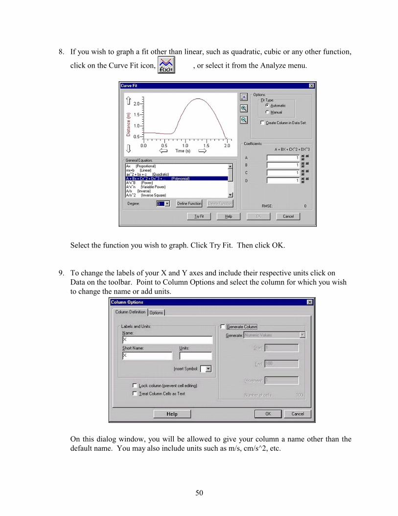
8. If you wish to graph a fit other than linear, such as quadratic, cubic or any other function,

click on the Curve Fit icon, , or select it from the Analyze menu.

Select the function you wish to graph. Click Try Fit. Then click OK.

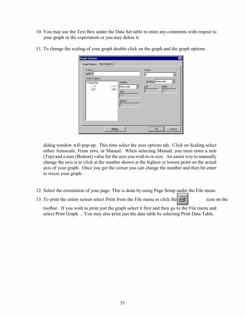
9. To change the labels of your X and Y axes and include their respective units click onData on the toolbar. Point to Column Options and select the column for which you wishto change the name or add units.

On this dialog window, you will be allowed to give your column a name other than thedefault name. You may also include units such as m/s, cm/s^2, etc.

50

10. You may use the Text Box under the Data Set table to enter any comments with respect toyour graph or the experiment or you may delete it.

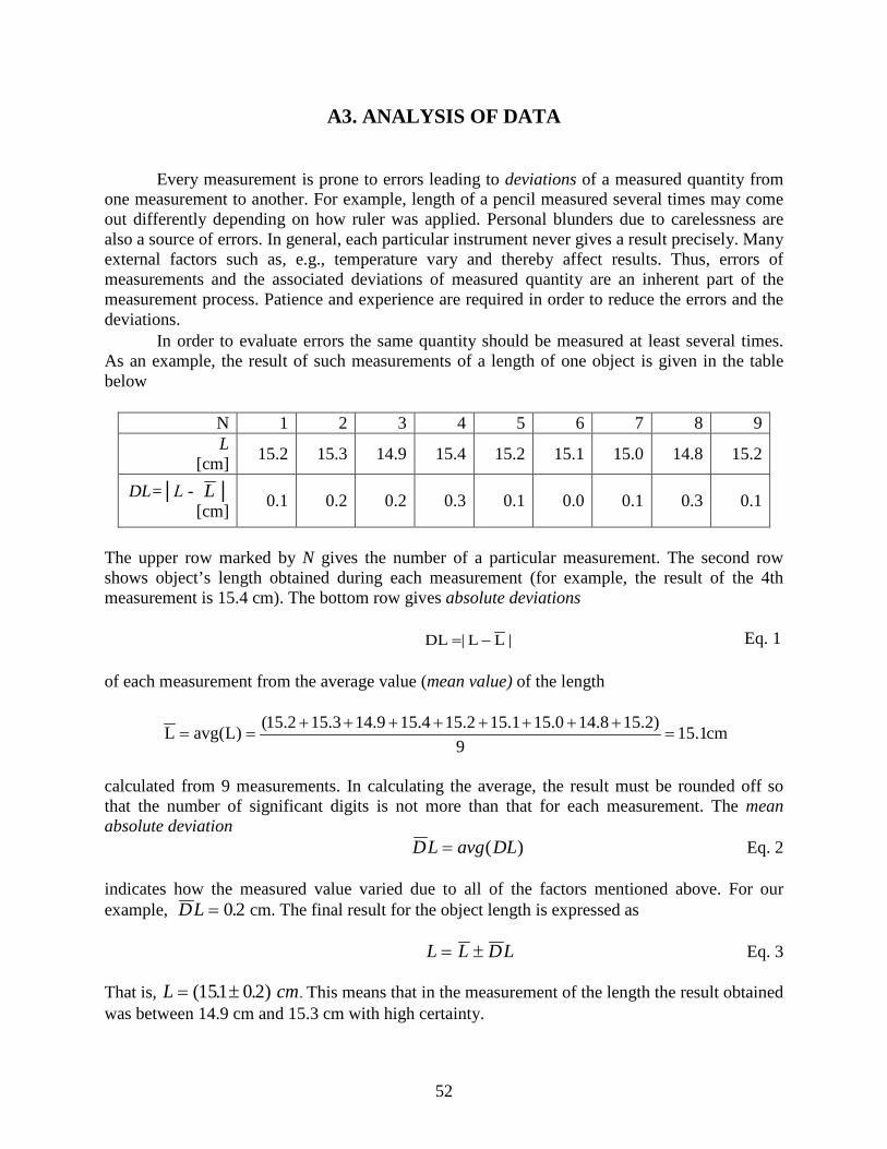
11. To change the scaling of your graph double click on the graph and the graph options

dialog window will pop-up. This time select the axes options tab. Click on Scaling selecteither Autoscale, From zero, or Manual. When selecting Manual, you must enter a min(Top) and a max (Bottom) value for the axis you wish to re-size. An easier way to manuallychange the axis is to click at the number shown at the highest or lowest point on the actualaxis of your graph. Once you get the cursor you can change the number and then hit enterto resize your graph.

12. Select the orientation of your page. This is done by using Page Setup under the File menu.

13. To print the entire screen select Print from the File menu or click the icon on the

toolbar. If you wish to print just the graph select it first and then go to the File menu andselect Print Graph… You may also print just the data table by selecting Print Data Table.

51

52

A3. ANALYSIS OF DATA Every measurement is prone to errors leading to deviations of a measured quantity from one measurement to another. For example, length of a pencil measured several times may come out differently depending on how ruler was applied. Personal blunders due to carelessness are also a source of errors. In general, each particular instrument never gives a result precisely. Many external factors such as, e.g., temperature vary and thereby affect results. Thus, errors of measurements and the associated deviations of measured quantity are an inherent part of the measurement process. Patience and experience are required in order to reduce the errors and the deviations.

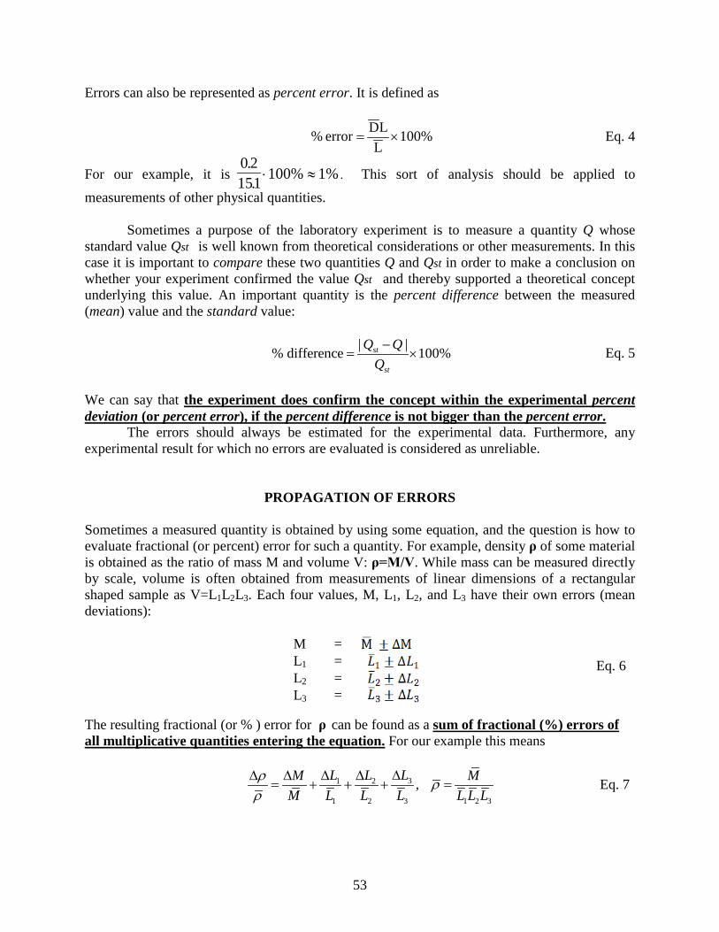
In order to evaluate errors the same quantity should be measured at least several times. As an example, the result of such measurements of a length of one object is given in the table below

N 1 2 3 4 5 6 7 8 9 L

[cm] 15.2 15.3 14.9 15.4 15.2 15.1 15.0 14.8 15.2

DL=│L - L │ [cm] 0.1 0.2 0.2 0.3 0.1 0.0 0.1 0.3 0.1

The upper row marked by N gives the number of a particular measurement. The second row shows object’s length obtained during each measurement (for example, the result of the 4th measurement is 15.4 cm). The bottom row gives absolute deviations

|LL|DL −= Eq. 1 of each measurement from the average value (mean value) of the length

cm1.159

)2.158.140.151.152.154.159.143.152.15()L(avgL =++++++++

==

calculated from 9 measurements. In calculating the average, the result must be rounded off so that the number of significant digits is not more than that for each measurement. The mean absolute deviation

DL avg DL= ( ) Eq. 2 indicates how the measured value varied due to all of the factors mentioned above. For our example, DL = 0 2. cm. The final result for the object length is expressed as

L L DL= ± Eq. 3

That is, L cm= ±( . . )151 0 2 . This means that in the measurement of the length the result obtained was between 14.9 cm and 15.3 cm with high certainty.

53

Errors can also be represented as percent error. It is defined as

%100LLD error % ×= Eq. 4

For our example, it is 0 2151 100% 1%

.. ⋅ ≈ . This sort of analysis should be applied to

measurements of other physical quantities.

Sometimes a purpose of the laboratory experiment is to measure a quantity Q whose standard value Qst is well known from theoretical considerations or other measurements. In this case it is important to compare these two quantities Q and Qst in order to make a conclusion on whether your experiment confirmed the value Qst and thereby supported a theoretical concept underlying this value. An important quantity is the percent difference between the measured (mean) value and the standard value:

| | % difference 100%st

st

Q QQ−

= × Eq. 5

We can say that

The errors should always be estimated for the experimental data. Furthermore, any experimental result for which no errors are evaluated is considered as unreliable.

the experiment does confirm the concept within the experimental percent deviation (or percent error), if the percent difference is not bigger than the percent error.

PROPAGATION OF ERRORS

Sometimes a measured quantity is obtained by using some equation, and the question is how to evaluate fractional (or percent) error for such a quantity. For example, density ρ of some material is obtained as the ratio of mass M and volume V: ρ=M/V. While mass can be measured directly by scale, volume is often obtained from measurements of linear dimensions of a rectangular shaped sample as V=L1L2L3. Each four values, M, L1, L2, and L3 have their own errors (mean deviations): The resulting fractional (or % ) error for ρ can be found as a sum of fractional (%) errors of all multiplicative quantities entering the equation.

For our example this means

31 2

1 2 3 1 2 3

, LL LM MM L L L L L L

ρ ρρ

∆∆ ∆∆ ∆= + + + = Eq. 7

M = L1 = L2 = L3 =

Eq. 6

54

Let us use particular measurements performed on a piece of wood of mass M with rectangular shape given by dimensions L1, L2 and L3 :

Then, the mean volume is 2.4.2.0.3.4=16 cm3 and the mean density becomes:

3 7.5 /16 0.47 cmgρ = =

The fractional error follows from Eq. 7 as

0.2 0.1 0.1 0.1 0.157.5 2.4 2.0 3.4

ρρ∆

= + + + =

That is, % error is 0.15.100%=15%, and the absolute error is 0.47.0.15 g/cm3 =0.07 g/cm3. The final answer for the density is

3 (0.47 0.07) cmgρ = ±

Similar procedure should be followed for other composite quantities.

STANDARD DEVIATION The method of estimating errors as the mean of the deviations shown in Eq. 2 to Eq. 4 can be improved by considering these deviations as some random variable. Then, the standard deviation of such variable from its mean is taken as the error. In general, the procedure becomes as follows:

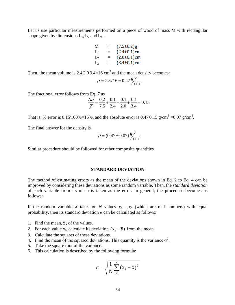
If the random variable X takes on N values x1,…,xN (which are real numbers) with equal probability, then its standard deviation σ can be calculated as follows:

1. Find the mean, x , of the values. 2. For each value xi, calculate its deviation )xx( i − from the mean. 3. Calculate the squares of these deviations. 4. Find the mean of the squared deviations. This quantity is the variance σ2. 5. Take the square root of the variance. 6. This calculation is described by the following formula:

M = L1 = L2 = L3 =

∑=

−=σN

1i

2i )xx(

N1

55

where x is the arithmetic mean of the values xi, defined as:

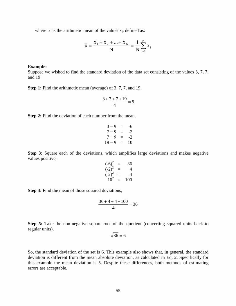
Example: Suppose we wished to find the standard deviation of the data set consisting of the values 3, 7, 7, and 19 Step 1: Find the arithmetic mean (average) of 3, 7, 7, and 19,

94

19773=

+++

Step 2: Find the deviation of each number from the mean,

3 − 9 = -6 7 − 9 = -2 7 − 9 = -2

19 − 9 = 10 Step 3: Square each of the deviations, which amplifies large deviations and makes negative values positive,

(-6)2 = 36 (-2)2 = 4 (-2)2 = 4 102 = 100

Step 4: Find the mean of those squared deviations,

Step 5: Take the non-negative square root of the quotient (converting squared units back to regular units),

So, the standard deviation of the set is 6. This example also shows that, in general, the standard deviation is different from the mean absolute deviation, as calculated in Eq. 2. Specifically for this example the mean deviation is 5. Despite these differences, both methods of estimating errors are acceptable.

∑=

=+++

=N

1ii

N21 xN1

Nx...xx

x

364

1004436=

+++

636 =