physik-department · physik-department the kondo exciton: non-equilibrium dynamics after a quantum...

PHYSIK-DEPARTMENT

The Kondo exciton: non-equilibrium dynamics after a quantum quench in the Anderson impurity model

Diplomarbeit

von

Markus Johannes Hanl

TECHNISCHE UNIVERSITÄT

MÜNCHEN

Contents

Abstract 3

1 Introduction 5

2 Model 7

2.1 Anderson Model . . . . . . . . . . . . . . . . . . . . . . . . . . . . . . 7

2.2 The Kondo Effect . . . . . . . . . . . . . . . . . . . . . . . . . . . . . 8

2.3 Excitonic Anderson Model . . . . . . . . . . . . . . . . . . . . . . . . 10

2.4 Kondo Model . . . . . . . . . . . . . . . . . . . . . . . . . . . . . . . 12

3 Experimental background 15

3.1 Experimental setup . . . . . . . . . . . . . . . . . . . . . . . . . . . . 15

3.2 Recent experimental work . . . . . . . . . . . . . . . . . . . . . . . . 17

4 Numerical calculations 19

4.1 NRG-method . . . . . . . . . . . . . . . . . . . . . . . . . . . . . . . 19

4.2 Energy flow diagram . . . . . . . . . . . . . . . . . . . . . . . . . . . 25

4.3 Calculations using NRG-results . . . . . . . . . . . . . . . . . . . . . 25

4.3.1 Absorption spectrum . . . . . . . . . . . . . . . . . . . . . . . 26

4.3.2 Occupations . . . . . . . . . . . . . . . . . . . . . . . . . . . . 27

4.3.3 Time-dependent NRG . . . . . . . . . . . . . . . . . . . . . . 28

4.3.4 Bulk magnetic field . . . . . . . . . . . . . . . . . . . . . . . . 29

5 Results 31

5.1 Occupation of Quantum Dot . . . . . . . . . . . . . . . . . . . . . . . 31

5.2 Time evolution of charge and spin after absorption . . . . . . . . . . 32

5.3 Absorption lineshape . . . . . . . . . . . . . . . . . . . . . . . . . . . 33

5.3.1 Large Detuning . . . . . . . . . . . . . . . . . . . . . . . . . . 37

5.3.2 Intermediate Detuning . . . . . . . . . . . . . . . . . . . . . . 40

5.3.3 Small Detuning . . . . . . . . . . . . . . . . . . . . . . . . . . 40

5.3.4 Temperature dependence . . . . . . . . . . . . . . . . . . . . . 44

5.3.5 Threshold frequency . . . . . . . . . . . . . . . . . . . . . . . 46

6 Conclusions 49

2 Contents

A Appendix 51A.1 Evaluation of the absorption lineshape in the strong-coupling-regime . 51A.2 Bulk magnetic field . . . . . . . . . . . . . . . . . . . . . . . . . . . . 53A.3 NRG parameters . . . . . . . . . . . . . . . . . . . . . . . . . . . . . 53

List of Figures 57

List of Tables 63

Bibliography 65

Acknowledgement 68

Abstract

The absorption of a photon by a semiconductor quantum dot (QD) can be con-sidered as a quantum quench, where a previously empty energy level in the QDgets suddenly occupied. In this thesis the non-equilibrium dynamics are examinedthat follow such a quantum quench. The studies consider mainly the absorptionlineshape and the time-evolution of spin and charge. Various quantities influencingthe lineshape are shortly discussed, too. The absorption spectrum can be dividedin three frequency regimes, corresponding to the three fixed points of the single-impurity Anderson Hamiltonian. The three frequency regimes of the absorptionlineshape are described both numerically and analytically, where special emphasisis put on the small detuning regime of the lineshape, which corresponds to an ex-citonic Kondo state in the dot. For such small frequencies, the lineshape behavesaccording to a power-law and diverges for very small detuning close to the thresholdfrequency, below which absorption abruptly ceases, resulting in a highly asymmet-ric lineshape. It is shown that the exponent of the power law divergence can betuned by magnetic field and can even take on opposite signs for different polariza-tion of the incident photon, which changes the shape of the absorption lineshapecompletely. The temperature-dependence of the lineshape is also studied. At tem-peratures smaller than the Kondo temperature TK , the lineshape is smeared out forfrequencies with energy lower than kBT . If temperature lies above TK , the peak-width of the absorption spectrum is given by the Korringa relaxation rate which issignificantly smaller than the frequency corresponding to kBT .

4 Abstract

Chapter 1

Introduction

Quantum dots (QD) are artificial objects with an extent somewhere between thenano- or the lower micrometer-scale, which can contain one up to several thousandelectrons. They are often referred to as artificial atoms, since they possess a system ofdiscrete energy levels, like atoms, and their size and shape can be defined artificiallywith means of nanofabrication technology. The interaction between the quantum dotand its environment can be described as a system of discrete energy levels coupledto a reservoir of electrons via tunneling-processes [1].

Due to the coupling between dot and reservoir, and the presence of interactionson the dot, electron correlations can arise. In dots that contain only a few electronsand at which the topmost discrete energy level below the Fermi-level of the reservoircontains only a single electron, below a characteristic crossover temperature TK

(the Kondo Temperature) the Kondo Effect can occur [2], a many-body effect thatscreens the local magnetic moment of the QD into a spin singlet by building up strongspin correlations between the dot spin and the spins of the reservoir electrons. TheKondo effect per se was discovered in the 1930’s as resistivity measurements of dilutemagnetic alloys showed unexpected results: as the metal is cooled down, resistivityincreases again below a certain temperature [3]. 30 years later J. Kondo explainedthis increase of resistivity with the existence of magnetic impurities in the metal thatenable scattering of the electrons at their magnetic moments [2]. His calculation,which was perturbative in the spin exchange coupling, yielded a diverging resistivityfor very low temperatures and could not be applied to the latter temperature regime.This was done by K. G. Wilson [4] who developed a non-perturbative method in1974 and 1975, the numerical renormalization group (NRG), and finally presenteda solution to this long-standing problem.

During the decades over which the theory of the Kondo effect was developed,experimentalists turned their interest to other physical problems. Due to the rapiddevelopment of nanofabrication technology over the last years, however, the Kondoeffect again has enjoyed much attention from the experimental side. With quantumdots it became possible to examine the Kondo effect in an artificial environment [5],[6], [7], to confirm theoretical predictions [8] and even to tune the parameters ofthe Kondo effect [9] as desired. So far, most experiments studying the Kondo effectwere transport measurements. With optical methods the Kondo effect has not beendetected yet, though experiments pointing in this direction have been performed

6 1. Introduction

[10], [11]. Theoretical work [12], [13] concerned with optics and the Kondo effect,mostly involved analytical methods.

Tying in with this work, the main goal of this thesis is to examine the opticalproperties of a QD, which is coupled to a fermionic reservoir and exhibits Kondophysics, by studying its absorption spectrum. Since the absorption of a photonby a QD can be considered as a quantum quench, this study is complemented bythe examination of the non-equilibrium dynamics following such a quantum quench;thereby giving insight into arguably the most extensively studied many-body prob-lem, a quantum impurity described by the Anderson model, and, closely related toit, the Kondo effect. We calculate these quantities using a method that had enoughpower to give a consistent explanation of the Kondo effect for the first time: theNRG-method.

In chapter 2 (model) several different models that are relevant for this thesis arediscussed. Apart from the Excitonic Anderson model on which the calculations ofthis thesis are based, and the Anderson model which is the underlying basis model,the Kondo model is also briefly introduced. Further, the Anderson model is used toillustrate the Kondo effect.

Chapter 3 (experimental background) summarizes the experimental work fore-going this thesis. The ultimative aim is to observe the Kondo effect with opticalmethods. Although this has not been achieved so far, there have been experimentsthat give hints that this aim is not far away and how it could be accomplished.

Chapter 4 (calculations) gives a detailed description of how the calculations forthis thesis were done. First, the NRG-method is introduced, in the improved formin which it is used today, where complete basis sets can be obtained. Moreover, thenumerical calculations of the most interesting quantities will be explained.

The results of the calculations are presented in Chapter 5 (results). The mostimportant part is the discussion of the absorption spectrum. It is shown how thetime evolution of charge and spin after photon-absorption is related to the spectrum.Furthermore, the dependence of the absorption lineshape on B-field and tempera-ture is examined and it is pointed out how information about physical quantitiesdescribing the system can be obtained from the lineshape.

In Chapter 6 the conclusions are presented and some special details concerningthe main part of the thesis are added as appendix.

Chapter 2

Model

2.1 Anderson Model

The Single Impurity Anderson Model (SIAM) describes an impurity in a metalor a single QD by modelling it as an energy level with a local interaction and ahybridization term that enables tunneling to a surrounding Fermi Reservoir (FR).

The Hamiltonian can be divided into three parts

H = HQD +Hc +Ht (2.1)

where the Hamiltonians on the r. h. s. consist of the following terms:

HQD =∑σ=↑,↓

εeσneσ + Une↑ne↓ (2.2)

Hc =∑~kσ

ε~kσc†~kσc~kσ (2.3)

Ht =√

Γ/πρ∑~kσ

(e†σc~kσ + h.c.) =√

Γ/πρ∑

σ

(e†σcσ + h.c.) (2.4)

with neσ = e†σeσ, cσ =∑

k ckσ

HQD is the Hamiltonian describing the QD. The first term describes the energyof the electrons on the e-level εeσ with respect to the Fermi Energy, where σ denotesthe spin of the electron. The second term accounts for the local Coulomb repulsionon the dot and is only non-zero if the dot is occupied by both electrons, which isprobed by the number-operators neσ

Hc describes the environment as a reservoir of many non-interacting electrons.Their energies εkσ are assumed to depend only on the absolute value of k with−D < εkσ < +D, where 2D is the bandwidth of the reservoir.

Ht connects the dot and the reservoir by allowing tunneling between e-level andFR. Tunneling processes are determined by the density of states ρ and Γ, of whichthe latter can be seen as a measure for the coupling strength between dot and

8 2. Model

εeσ + U

εeσ

εF

2e−

V

Figure 2.1: Single Impurity Anderson Model. The dot is coupled to a Fermionicreservoir (indicated blue). The local level εeσ is separated from the reservoir byCoulomb barriers (indicated by thick black lines) through which electrons can tunnel.Tunneling strength is determined by the transition matrix element V . If the locallevel is occupied by two electrons their energy is increased by U due to Coulombrepulsion

reservoir. The prefactor of the Hamiltonian√

Γ/πρ is determined by the hybridiza-

tion matrix element between dot and reservoir√

Γ/πρ = 〈ψQD|H|ψc〉 where 〈ψQD|and |ψc〉 are electron wavefunctions on the dot and in the reservoir, respectively.Coupling does not depend on k, i. e. it is assumed that all states of the reservoirare coupled to the dot with equal strength. For this reason the tunneling Hamil-tonian Ht depends only on the combination of operators cσ =

∑k ckσ (see Eq. (2.4)).

The above model was proposed by P. W. Anderson [14] in the 1960s and is widelyused to model impurities in metals or Quantum Dots. It can easily be generalized toseveral local levels and reservoirs, however the problems arising from these modelscan be very difficult to solve. These general Anderson models are subject of currentresearch, but are not considered in this thesis.

2.2 The Kondo Effect

The Kondo Effect emerges when a localized spin degree of freedom, provided e.g.by a single molecule, a magnetic impurity or an unpaired electron in a quantumdot, is coupled to a continuous reservoir of electrons. The Kondo Effect is a many-body effect where the spin of the localized single electron is totally screened to aneffective spin singlet by electrons from the surrounding reservoir. This screening setsin once the temperature T crosses below a characteristic temperature, the Kondotemperature TK . There are several ways to determine TK . In this thesis, it wasdetermined according to χ0 = 1/4TK [15], where χ0 is the magnetic susceptibility

2.2 The Kondo Effect 9

V V

V V

(a)

(b)

Figure 2.2: Virtual processes that result in a spin-flipped state. (a) An electrontunnels from the reservoir onto the dot into a virtual excited state. The electronthat had previously occupied the dot tunnels back and the dot-electron is flipped.(b) An electron from the dot tunnels into the reservoir and an electron with oppositespin tunnels back.

at T = 0, which was calculated with NRG. This definition is very convenient foraccurate numerical evaluation. In situations in which its use was very unpractical,the formula [16] (see also (2.4))

TK =√

ΓU/2e−π|εe(εe+U)|/(2UΓ), (2.5)

was used instead, which gives essentially equivalent results.The electron on the e-level couples to the FR via tunneling. Through tunneling

processes it is possible that a spin flip occurs on the dot; the two lowest-order virtualprocesses at which the spin is flipped are shown in Fig. 2.2. In Fig. 2.2a an electrontunnels from the reservoir to the dot and an electron from the dot tunnels back. Thisprocess requires the energy (εeσ) + U . Since this energy is not freely available, theprocess must occur at a time scale of ∆t ≈ ~(εeσ +U) at which energy conservationcan be violated. If the electron tunneling back to the e-level has different spin thanthe one tunneling out, the spin of the QD-electron is flipped. In Fig. 2.2b the electrontunnels from the e-level into the FR and one electron from the FR tunnels back, therelevant time scale is given by ∆t ≈ ~|εeσ|.

At energies below TK (kB = ~ = µB = 1 throughout the thesis) the systemis in a state where electrons from the reservoir continuously tunnel from the FRonto the local level and back. At these low energy states the spin-flips induced byvirtual processes happen so often, that the spin of the local electron gets screenedand forms a spin singlet. However this spin-screening is mainly caused by higherorder processes, like the one shown in Fig. 2.3 at which the spin-flipped state is an

10 2. Model

ε‚

spin-flippedvirtual state

1 2 3 4 5

Figure 2.3: Example of a fourth order virtual process that contributes to the spin-screening at a Kondo state. Higher order virtual processes with a virtual spin-flippedintermediate state produce the spin-screening that is typical for the Kondo-regime.

intermediate state of the virtual processes.

Because of this frequent tunneling, which involves a variety of virtual states, thedensity of states drastically increases around the ground state energy, resulting inthe so called Kondo-peak in the local density of states (LDOS). This can be seen inFig. 2.4 where the local density of states A(ω) is shown within a schematic figureof the Anderson model. The smaller peaks of the LDOS at the local levels aredetermined by the hybridization between local level and reservoir and have width Γ.

2.3 Excitonic Anderson Model

To calculate the absorption spectrum, the Excitonic Anderson Model is used, anextension of the Anderson Model (2.1). At an absorption process, an incident photonis absorbed by a semiconductor quantum dot and creates a particle-hole pair. Thehole is thereby created in the valence level, which is far below the local level and notconnected to the reservoir. Whereas a static quantum dot with a single local levelcan usually be described by the Anderson Model, this model must now be extendedfor a proper description of the absorption process, where the extension must containthe energy of the hole, the excitonic Coulomb attraction and the interaction betweenphoton and dot. The new Hamiltonian for the Excitonic Anderson Model (EAM) isthen given by:

HEAM = HQD +Hc +Ht +Hh +Heh +HL (2.6)

Hh =∑

σ

εhσ + Uhnh↑nh↓ (2.7)

Heh = −∑σ,σ′

Uehneσ(1− nhσ′) (2.8)

HL =∑

k

(γkake†σh

†σe−iωkt + h.c.). (2.9)

2.3 Excitonic Anderson Model 11

εeσ + U

εeσ

εF

A(ω)

Figure 2.4: Kondo-peak in the local density of states. For T < TK the variety ofpossible tunneling processes drastically increases the local density of states A(ω)(red line) around the Fermi energy. This becomes visible as a sharp resonance inthe local density of states. The LDOS also has smaller peaks at the local levels(Hubbard-side-peaks) which have width Γ.

Hh is thereby the Hamiltonian for the valence level where the first term describesthe energy of the holes and the second term the Coulomb repulsion of two holesin the valence level. Heh accounts for the Coulomb attraction between electrons inthe local level and holes in the valence level. HL describes the interaction betweenphoton and dot, it creates an electron at the local level and a hole at the valencelevel, by e†σ and h†σ, respectively. ak annihilates a photon with wave vector k andγk = γ is the coupling strength of the photon to the two-level system which will beassumed to be independent of k. Since the quantization of the photon field will notbe relevant for the discussions below, HL can be written as:

HL = γ(e†σh†σ + h.c.). (2.10)

In this thesis, only processes are examined where one hole is created in a previouslyfully occupied valence level. For this special problem, it is simpler to think in termsof two different Hamiltonians, H i and Hf , one for the initial state before absorptionand one for the final state with Coulomb attraction. Therefore all further discussionswill be presented in terms of H i and Hf .

The initial and the final Hamiltonian consist of three parts:

H i/f = Hi/fQD +Hc +Ht (2.11)

12 2. Model

⇓

σ+

(a) (b)

εieσ

εfeσ

εhσεhσ

UehεF

Figure 2.5: Schematic figure the excitonic Anderson model and the correspondingabsorption process. Due to photon absorption a hole is created in the valence levelwhich pulls the e-level down by the electron-hole attraction Ueh. After absorptionthe position of the e-level is below the Fermi-level so that the electron is stabilizedagainst flowing away into the FR, but can build out hybridization states.

HaQD =

∑σ

εaeσneσ + Une↑ne↓ + δafεhσ (a = i, f) (2.12)

Hc =∑kσ

εkσc†kσckσ (2.13)

Ht =√

Γ/πρ∑

σ

(e†σcσ + h.c.). (2.14)

These Hamiltonians are equal to the SIAM-Hamiltonian, however, they differ in(i) the position of their e-levels (εi

eσ and εfeσ = εi

eσ − Ueh), where the e-level of thefinal Hamiltonian is pulled down by the excitonic Coulomb attraction and (ii) inan additional term of δafεhσ that accounts for the energy of the hole. Due to theKronecker-delta, δaf , this term is only “activated” if the system is in its final state(see Fig. 2.5).

If a magnetic field is applied parallel to the growth-direction of the QD, whichwill be the case at some of the calculations presented later, the local level splits intwo separate levels, εeσ = εe + 1

2σgeB, and the energy of the electrons in the FR

changes according to εkσ = εk + 12σgcB where ge and gc are the g-factors of the

electrons on the dot or in the FR, respectively.

2.4 Kondo Model

Although the Kondo model is not used for the examinations described in this the-sis, it will briefly be mentioned here. This is justified because as the AndersonModel, this model is widely used to describe impurity problems and is related to

2.4 Kondo Model 13

the Anderson Model in many ways. The idea behind the Kondo model is that asingle magnetic moment ~S interacts with the accumulated spin of the FR electrons~s = 1

2

∑kk′σσ′ c

†kσ~τσσ

′ckσ′ . This causes an effective spin-spin-coupling ~S · ~s and leadsto the following Hamiltonian:

HK = 2J ~S · ~s+∑kσ

εkc†kσckσ, (2.15)

where the coupling constant J determines the coupling strength. Since the local levelinteracts with the Fermi-sea only via spin-spin-coupling, this model can describe onlyspin-, but no charge-fluctuations.

Note that the Kondo model is more “elementary” than the Anderson model. TheKondo effect can be explained in the same way as in (2.2): virtual spin-flipped statesscreen the local moment. Here however, spin-flips are only possible without chargefluctuations. The Kondo temperature can be determined by the so called poorman’s scaling method [17]. Calculations to third order in J yield for the Kondotemperature

TK ∼ DKM |2Jρ|2e−1/2Jρ, (2.16)

where DKM is the effective bandwidth of the Kondo model which is proportional tothe Coulomb energy of the Anderson model U .

The Schrieffer-Wolff transformation [18], maps the Single Impurity Andersonmodel on the Kondo model and yields a relation between J and Γ:

J(Γ) = − Γ

πρ

U

(U + εeσ)εeσ

. (2.17)

The Kondo temperature for the Anderson model (Eq. (2.5)) can then be obtainedfrom Eq. (2.16) and Eq. (2.17).

14 2. Model

Chapter 3

Experimental background

3.1 Experimental setup

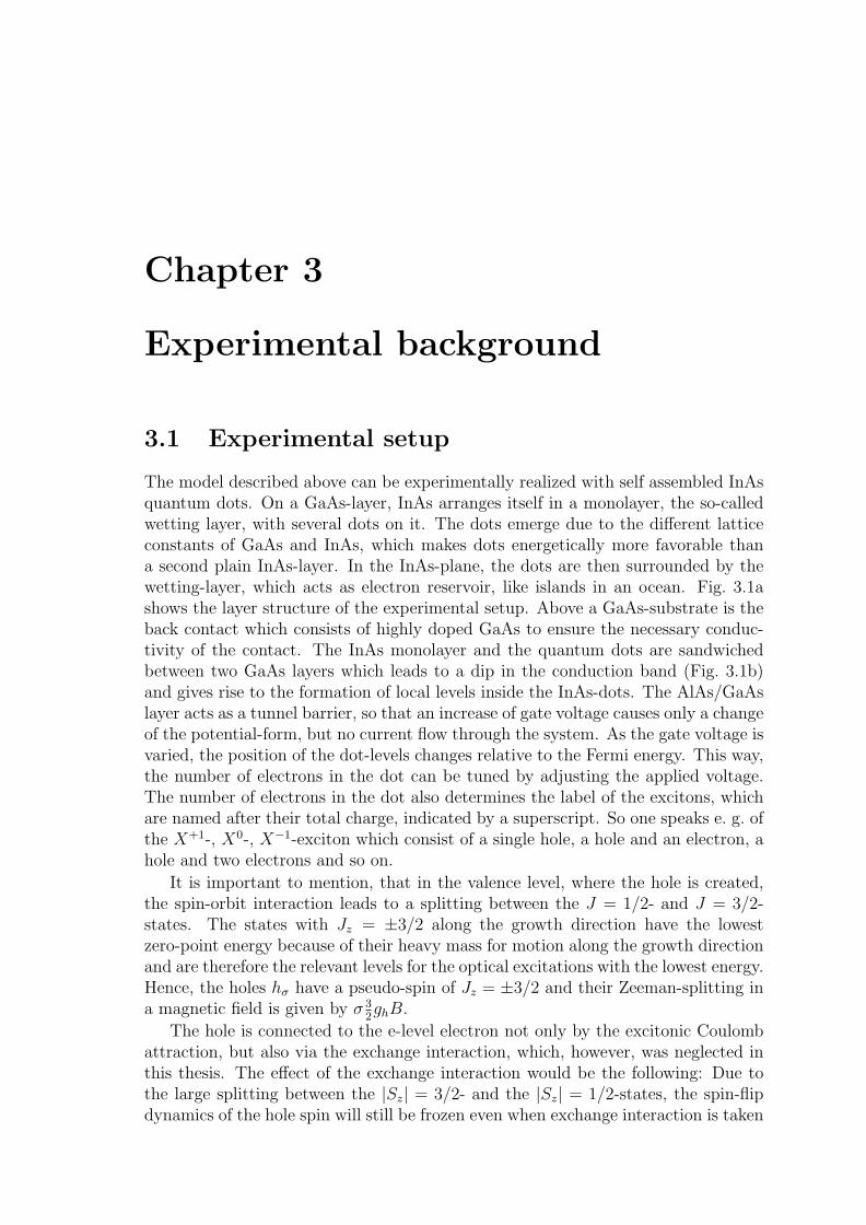
The model described above can be experimentally realized with self assembled InAsquantum dots. On a GaAs-layer, InAs arranges itself in a monolayer, the so-calledwetting layer, with several dots on it. The dots emerge due to the different latticeconstants of GaAs and InAs, which makes dots energetically more favorable thana second plain InAs-layer. In the InAs-plane, the dots are then surrounded by thewetting-layer, which acts as electron reservoir, like islands in an ocean. Fig. 3.1ashows the layer structure of the experimental setup. Above a GaAs-substrate is theback contact which consists of highly doped GaAs to ensure the necessary conduc-tivity of the contact. The InAs monolayer and the quantum dots are sandwichedbetween two GaAs layers which leads to a dip in the conduction band (Fig. 3.1b)and gives rise to the formation of local levels inside the InAs-dots. The AlAs/GaAslayer acts as a tunnel barrier, so that an increase of gate voltage causes only a changeof the potential-form, but no current flow through the system. As the gate voltage isvaried, the position of the dot-levels changes relative to the Fermi energy. This way,the number of electrons in the dot can be tuned by adjusting the applied voltage.The number of electrons in the dot also determines the label of the excitons, whichare named after their total charge, indicated by a superscript. So one speaks e. g. ofthe X+1-, X0-, X−1-exciton which consist of a single hole, a hole and an electron, ahole and two electrons and so on.

It is important to mention, that in the valence level, where the hole is created,the spin-orbit interaction leads to a splitting between the J = 1/2- and J = 3/2-states. The states with Jz = ±3/2 along the growth direction have the lowestzero-point energy because of their heavy mass for motion along the growth directionand are therefore the relevant levels for the optical excitations with the lowest energy.Hence, the holes hσ have a pseudo-spin of Jz = ±3/2 and their Zeeman-splitting ina magnetic field is given by σ 3

2ghB.

The hole is connected to the e-level electron not only by the excitonic Coulombattraction, but also via the exchange interaction, which, however, was neglected inthis thesis. The effect of the exchange interaction would be the following: Due tothe large splitting between the |Sz| = 3/2- and the |Sz| = 1/2-states, the spin-flipdynamics of the hole spin will still be frozen even when exchange interaction is taken

16 3. Experimental background

subs

trat

eG

aAs

back

con

tact

n-do

ped

GaA

stu

nnel

Bar

rier

GaA

s

GaA

s-la

yer

tunn

el b

arrie

rA

lAs/

GaA

s

InAs quantum dots

GaA

s-la

yer

gate

(a)

(b)

V 1g

V 2g

Figure 3.1: Layer structure and its band diagram. Picture from [19]. (a) Layerstructure of the experimental setup. (b) The band diagram of the layer structure isshown for two different gate voltages V 1

g and V 2g . Increasing the gate voltage changes

the number of electrons in the dot.

into account, so that the exchange interaction reduces to JehSzeS

zh. This acts on the

e-level like a magnetic field of strength 32σJeh. By applying a small magnetic field

in the opposite direction, the “static exchange field” can be fully compensated, sothat the predictions of this thesis remain unchanged when a constant term is addedto the magnetic field: B → B − 3

2σJeh.

In case it is nevertheless necessary to experimentally avoid the exchange inter-action for some reasons, it can be eliminated in two ways. One possibility is to usethe single-hole charged QD as the initial state; experiments on single QDs whichare embedded in n-type Schottky structures have already shown that such a chargedstate can have lifetimes well above 100 µsec. An additional photon-absorption cre-ates the X+1 trion, which consists of two holes and an electron in a local level. Theholes form a singlet and due to their spins cancelling each other, their exchangeinteraction with the local electron vanishes. The other way to avoid the exchangeinteraction, is to use coupled quantum dots with indirect excitons where electronand hole have wave-functions with vanishing spatial overlap.

3.2 Recent experimental work 17

3.2 Recent experimental work

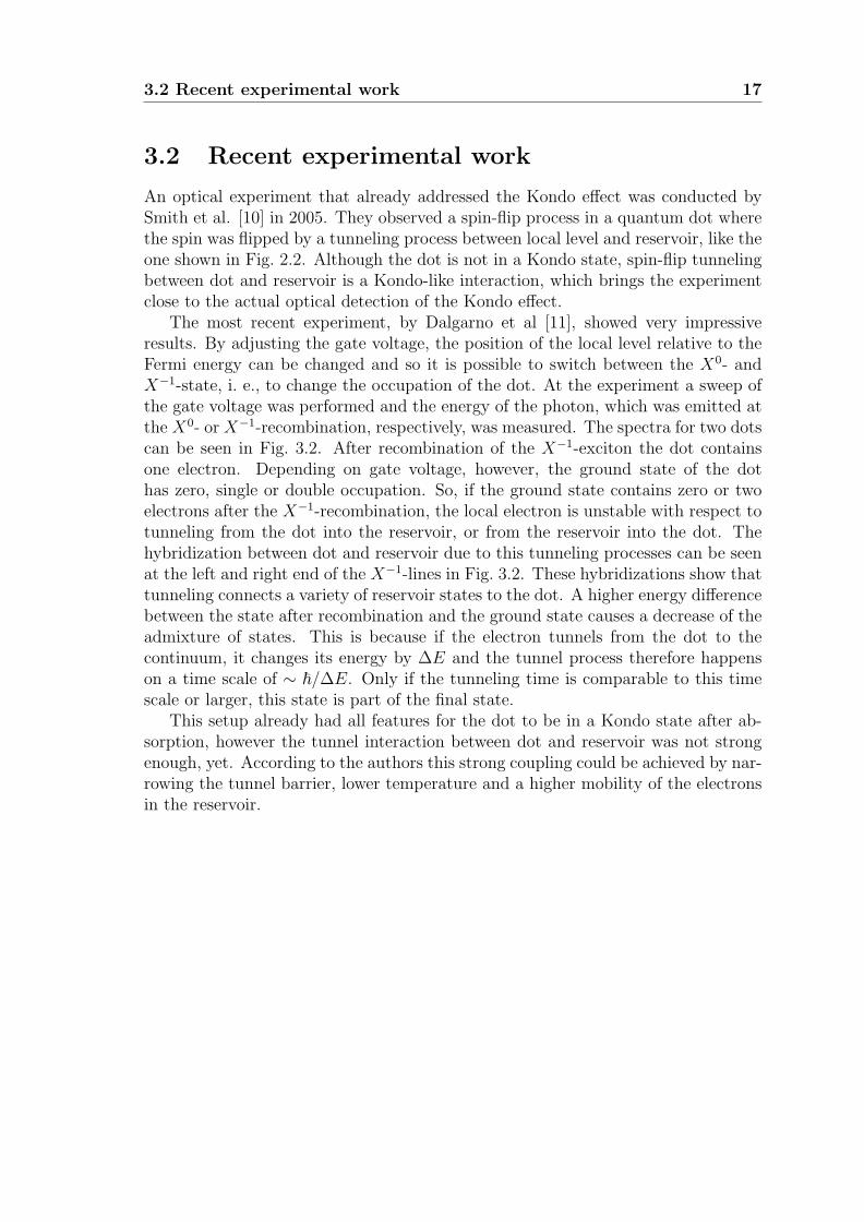
An optical experiment that already addressed the Kondo effect was conducted bySmith et al. [10] in 2005. They observed a spin-flip process in a quantum dot wherethe spin was flipped by a tunneling process between local level and reservoir, like theone shown in Fig. 2.2. Although the dot is not in a Kondo state, spin-flip tunnelingbetween dot and reservoir is a Kondo-like interaction, which brings the experimentclose to the actual optical detection of the Kondo effect.

The most recent experiment, by Dalgarno et al [11], showed very impressiveresults. By adjusting the gate voltage, the position of the local level relative to theFermi energy can be changed and so it is possible to switch between the X0- andX−1-state, i. e., to change the occupation of the dot. At the experiment a sweep ofthe gate voltage was performed and the energy of the photon, which was emitted atthe X0- or X−1-recombination, respectively, was measured. The spectra for two dotscan be seen in Fig. 3.2. After recombination of the X−1-exciton the dot containsone electron. Depending on gate voltage, however, the ground state of the dothas zero, single or double occupation. So, if the ground state contains zero or twoelectrons after the X−1-recombination, the local electron is unstable with respect totunneling from the dot into the reservoir, or from the reservoir into the dot. Thehybridization between dot and reservoir due to this tunneling processes can be seenat the left and right end of the X−1-lines in Fig. 3.2. These hybridizations show thattunneling connects a variety of reservoir states to the dot. A higher energy differencebetween the state after recombination and the ground state causes a decrease of theadmixture of states. This is because if the electron tunnels from the dot to thecontinuum, it changes its energy by ∆E and the tunnel process therefore happenson a time scale of ∼ ~/∆E. Only if the tunneling time is comparable to this timescale or larger, this state is part of the final state.

This setup already had all features for the dot to be in a Kondo state after ab-sorption, however the tunnel interaction between dot and reservoir was not strongenough, yet. According to the authors this strong coupling could be achieved by nar-rowing the tunnel barrier, lower temperature and a higher mobility of the electronsin the reservoir.

18 3. Experimental background

- 2 . 1 - 2 . 0 - 1 . 9 - 1 . 8 - 1 . 7

1 . 3 6 0

1 . 3 6 5 ( a )

X 0

Energ

y (eV

)

X 1 -

- 0 . 2 - 0 . 1 0 . 0 0 . 1

1 . 3 6 8

1 . 3 7 1

1 . 3 7 4 ( b )

Energ

y (eV

)

G a t e V o l t a g e ( V )

X 1 -

X 0

Figure 3.2: Measured photoluminescence intensity vs. gate voltage Vg from twoInAs/GaAs quantum dots at nominally 4 K. The colors indicate the detector counts,the white solid lines mark the X0 to X−1-transition. Picture: courtesy of P. Dal-garno.

Chapter 4

Numerical calculations

In the 1970’s K. G. Wilson developed the NRG method to solve the Kondo Hamil-tonian and explain the Kondo Problem [4]. Developing an alternative method toperturbation theory was necessary to make energy scales below TK accessible. Inthe following years, the NRG was adapted to several other impurity models. Oneof these models is the widely used Anderson model as described in [14]. This modelhas been solved with the NRG-method by Krishna-Murthy et al. in 1980 [20].

4.1 NRG-method

The NRG method is an iterative procedure, that numerically diagonalizes the Hamil-tonians of quantum impurity models like the Anderson- or the Kondo-Hamiltonian.

For calculations concerning the excitonic Anderson model that include both theinitial and final Hamiltonian, the NRG-method is applied twice, once with the e-levelat position εi

eσ and once at εfeσ = εi

eσ − Ueh.

Thus, for our purposes it is sufficient to take the Single Impurity Anderson Modelto describe the NRG method.

The SIAM-Hamiltonian is given by the following expression:

H = HQD +Hc +Ht (4.1)

HQD =∑

σ

εeσneσ + Une↑ne↓ (4.2)

Hc =∑~kσ

ε~kσc†~kσc~kσ (4.3)

Ht =√

Γ/πρ∑

σ

(e†σcσ + h.c.). (4.4)

20 4. Numerical calculations

It can be written in a form with dimensionless parameters:

H = D

(∫ 1

−1

k∑

σ

a†kσakσdk

+1

D

(εeσ +

1

2U

)∑σ

e†σeσ +1

2

U

D

(∑σ

e†σeσ − 1

)2

+

(Γ

πD

)1/2 ∫ 1

−1

dk∑

σ

(a†kσeσ + e†σakσ

)),

(4.5)

where k ≡ ε/D is a dimensionless parameter (not the wave-vector ~k), which describesthe energy normalized by bandwidth and akσ ≡

√Daεσ. akσ (a†kσ) and aεσ (a†εσ) are

annihilation (creation) operators that annihilate (create) an electron in the FR whichhas energy k (or ε, respectively) and spin σ.

To calculate properties of the combined system QD-reservoir it is necessary todiscretize the energy spectrum in an efficient way to reduce computation costs.Therefore, one uses a logarithmic discretization scheme. This is due to the factsthat: (i) all energy scales have to be taken into account for the calculation of physicalproperties and (ii) low energies play a major role in impurity systems and logarithmicdiscretization has a finer resolution for low energies.

To discretize the energy spectrum as described above, a parameter Λ > 1 isintroduced and the energy spectrum is divided into intervals determined by Λ, asshown in Fig. 4.1, where the nth interval extends from Λ−(n+1) to Λ−n. Withinthese intervals one can set up a Fourier series which constitutes a complete set oforthonormal functions and which therefore spans the whole k space:

ψ±np(k) ≡

{Λn/2

(1−Λ−1)1/2 e±iωnpk if Λ−(n+1) < ±k < Λ−n

0 if ±k is outside the above interval(4.6)

n = 0, 1, 2, ... is the interval index, p is the Fourier harmonic index and takes integervalues from −∞ to +∞. Each interval occurs twice, once for positive and once fornegative k-values. The superscript ± indicates whether one refers to the intervalin the positive or in the negative k-part. ωn is the Fourier frequency for the nthinterval and is given by:

ωn ≡2π

Λ−n − Λ−(n+1)=

2πΛn

1− Λ−1. (4.7)

The operators akσ can now be expressed in this basis.

akσ =∑np

[anpσψ+np(k) + bnpσψ

−np(k)], (4.8)

anpσ =

∫ +1

−1

dk[ψ+np(k)]

∗akσ, bnpσ =

∫ +1

−1

dk[ψ−np(k)]∗akσ. (4.9)

The anpσ- and bnpσ-operators constitute a complete set of independent and discrete

electron operators which fulfill standard anti-commutation rules: [anpσ, a†n′p′σ′ ]+ =

δn,n′δp,p′δσ,σ′ .

4.1 NRG-method 21

/

1

-1

(a)

...

/

1

-1

(b)

...

Figure 4.1: Logarithmic discretization of the energy spectrum of the reservoir. Pic-ture from [21]. (a) The impurity (red dot) couples to the whole reservoir wherecoupling strength does not depend on energy. The reservoir is logarithmically di-vided into ever smaller intervals indicated by dashed lines. (b) Each energy intervalis represented by a single energy value which is taken to be the mean value of theinterval. The coupling strength to a discrete energy value is then proportional tothe interval size and therefore decreases for smaller energy values.

With these operators, the Hamiltonian (4.5) can be expressed as a discrete sum.To do this, one uses the following relations, which can easily be verified:

∫ +1

−1

k∑

σ

a†kσakσdk =1

2

(1 + Λ−1

)∑n,p,σ

Λ−n(a†npσanpσ − b†npσbnpσ

)+

1− Λ−1

2πi

∑n,p6=p′,σ

(a†npσanp′σ − b†npσbnp′σexp

(2πi(p′ − p)

1− Λ−1

)),

∫ +1

−1

∑σ

akσdk = (1− Λ)1/2∑n,σ

Λ−n/2(an0σ + bn0σ).

(4.10)

Inserting Eq. (4.10) in Eq. (4.5) reveals that the impurity couples only to the op-erators an0σ and bn0σ directly. The operators anpσ and bnpσ with p 6= 0 are onlyconnected indirectly to the impurity by the second term in Eq. (4.10) which cou-ples them to an0σ and bn0σ. Since this term has a prefactor of (1− Λ−1) /2π, thisindirect coupling will be very small if Λ is close to 1. Because of that the terms inEq. (4.10) with anpσ and bnpσ can be dropped for p 6= 0. This turns out to be a goodapproximation for sufficiently small Λ, e. g. Λ ≤ 3.

By using this approximation, dropping the subscript “0” of the operators an0σ


and bn0σ and introducing the operators

f0σ =

[1

2

(1− Λ−1

)]1/2 ∞∑n=0

Λ−n/2∑

σ

(anσ + bnσ) ≡ 1√2

∫ +1

−1

dkakσ, (4.11)

with [f0σ, f†0σ′ ] = δσ,σ′ the Hamiltonian can be now written as:

H

D=

1

2

(1 + Λ−1

) ∞∑n=0

Λ−n(a†nσanσ − b†nσbnσ

)+

1

D

(εeσ +

1

2U

)e†σeσ +

1

2

U

D

(e†σeσ − 1

)2+

(2Γ

πD

)1/2 (f †0σeσ + e†σf0σ

).

(4.12)

Now one performs a unitary transformation from the operators (anσ, bnσ) to anew orthonormal set of operators fnσ at which f0σ remain unchanged. Because theterm in Eq. (4.12) that describes the kinetic energy of the electrons is diagonal in(anσ, bnσ), a transformation will create non-diagonal matrix elements, i. e. a trans-formation will couple the operators (fnσ) to one another. The trick is to choose atransformation which couples fnσ only to its nearest neighbors f(n±1)σ. After thistransformation [20] one gets the following expression, the so-called Hopping Hamil-tonian:

H

D=

1

2

(1 + Λ−1

) ∞∑n=0

Λ−n/2ξn∑

σ

[f †nσf(n+1)σ + f †(n+1)σfnσ

]+

1

D

(εeσ +

1

2U

)∑σ

e†σeσ +1

2

U

D

(∑σ

e†σeσ − 1

)2

+

(2Γ

πD

)1/2∑σ

(f †0σeσ + e†σf0σ

),

(4.13)

with

ξn = (1− Λ−n−1)(1− Λ−2n−1)−1/2(1− Λ−2n−3)−1/2, (4.14)

which converge to one in the limit of large n.

This Hamiltonian can be represented by a semi-infinite chain, the so-called Wil-son chain (Fig. 4.1). The chain starts with the impurity which is then coupled to thesite that corresponds to the eigenstate of the operators f †0σ and f0σ. This site is thencoupled to the site that corresponds to the eigenstate of f1σ, this one is coupled tothe f2-site and so on. As n increases, the coupling becomes proportional to Λ−n/2,it decays exponentially.

4.1 NRG-method 23

......

site

V ∝ Λ−1 2 ∝ Λ−1 ∝ Λ−(n+1) 2/ /

0 1 2 n n+1im-

purity

Figure 4.2: Wilson chain. The original Hamiltonian can be mapped on a semi-infinitechain Hamiltonian that starts with the impurity and where each site is connectedonly to its nearest neighbors by exponentially decreasing coupling strength. Due tothe decreasing coupling strength, the contribution of new sites goes to zero for largen.

With help of the Hamiltonians HN ,

HN ≡ Λ(N−1)/2

[N−1∑n=0

Λ−n/2ξn∑

σ

(f †nσf(n+1)σ + f †(n+1)σfnσ

)+ Γ1/2

∑σ

(f †0σeσ + e†σf0σ

)

+δe∑

σ

e†σeσ + U

(∑σ

e†σeσ − 1

)2 ,

(4.15)

that have a finite number of elements determined by N , the Hopping Hamiltoniancan be expressed as:

H = limN→∞

1

2

(1 + Λ−1

)DΛ−(N−1)/2HN , (4.16)

where the following constants were defined for simplification of Eq. (4.15):

δe ≡(

2

1 + Λ−1

)1

D

(εeσ +

1

2U

)≡ εe + U (4.17)

U ≡(

2

1 + Λ−1

)U

2D(4.18)

Γ ≡(

2

1 + Λ−1

)22Γ

πD. (4.19)

From Eq. (4.15) it follows that the Hamiltonians HN fulfill the recursion relation:

HN+1 = Λ1/2HN + ξN(f †NσfN+1σ + f †N+1σfNσ). (4.20)

Due to this recursion relation it is possible to create a recursive procedure fromwhich one can calculate the Eigenstates and the corresponding energies of HN+1, ifthe ones from HN are known.


To apply this procedure on the Hamiltonian one needs a set of eigenstates andenergy levels as a starting point. These can be obtained from

H0 = Λ−1/2[δee

†σeσ + Γ1/2(f †0σeσ + e†σf0σ) + U(e†σeσ − 1)2

]. (4.21)

At the recursive procedure |l, N〉 is the eigenstate of HN with energy-index l. If thestates |l, N〉 are known, one also knows the matrix elements 〈l, N |f †nσ|l′, N〉

With the states |l, N〉 it is possible to create the following new states:

|1, l, N〉 ≡ |l, N〉|2, l, N〉 ≡ f †N+1↑|l, N〉|3, l, N〉 ≡ f †N+1↓|l, N〉|4, l, N〉 ≡ f †N+1↑f

†N+1↓|l, N〉.

(4.22)

|i, l, N〉 (i = 1, 2, 3, 4) are an orthonormal basis for HN+1 and thus it is possible tocalculate its matrix elements 〈i′, l′, N |HN+1|i, l, N〉.

At each Hamiltonian HN+1 the term ξN∑

σ(f †NσfN+1σ + f †N+1σfNσ) adds a newsite to the Wilson chain that corresponds to an energy scale of Λ−N/2. Once theenergy scale of interest is reached, one stops applying the recursion relation and theobtained eigenstates and -energies can be used for further calculations.

As can be seen from Eq. (4.22) every time a new site is added to the Wilsonchain, the Hilbert space of the system is multiplied by 4, the dimension of the statespace of a site. To prevent the Hilbert space from growing exponentially with thenumber of sites, only the MK states that are lowest in energy are kept at each it-eration, where MK is typically chosen between 256 and 1024. Calculation time isfurther reduced by using some symmetries of the system, namely the fact, that thez-component of the total spin and the particle number are conserved, so that thestate space can be divided into subspaces that correspond to the quantum numbersof the problem.

There have been developments in the past years how the NRG-determined eigen-states are used best to calculate physical quantities. The first approach by Wilsonwas to use only the states of iteration n which corresponds to the energy scale Λ−n/2

to describe the physics at that scale. This step involves several approximations whichare necessary to handle the problem that the states obtained at one NRG-iterationdo not constitute a complete basis.

A newer concept, which was developed by [22], [23] and [24] was used in thisthesis. There, the idea is not only to make use of the states at a certain NRG-iteration, but to use an approximate but complete basis set of states. The trickto obtain such a basis, is to keep the states that are discarded after each iteration(see Fig. 4.1ab). When the iterations are completed, there are only discarded statesleft, which form a complete set of basis states (Fig. 4.1b, right part). Eigenstatesat iteration n < N are then considered as dN−n-fold degenerate eigenstates of thefull chain. The first clean application of the complete state space to the calculationof spectral correlation functions was given in [24]. Specifically, it includes an ex-pansion of the density matrix in the complete state space, which is crucial for finitetemperature calculations.

4.2 Energy flow diagram 25

(a) (b)

10 2 3 N

...

4 N-1

discarded

kept

n

En

10 2 3 N

...

4 N-1 n

En

⊗|σ⊗|σ

⊗|σ ...

... ⊗|σ

⊗|σ

⊗|σ

...

Figure 4.3: Obtaining a complete basis set of states. Picture from [25]. The figuresshow the energy spectra for each iteration. (a) As soon as the dimension of theHilbert Space exceeds a certain number MK , only the lowest MK states are kept atan iteration, the rest of the states is discarded. (b) The discarded states at iterationn are taken to be (N-n)-fold degenerate, indicated by |σ〉 that represents the Hilbertspace of one site. After the total number of iterations N a set of complete basisstates remains (shown after the last iteration).

4.2 Energy flow diagram

To get insight which energy scales determine the physics of the system, it is in-structive to examine how the energy spectrum of the kept-states, which are usedfor the iterative diagonalization, varies with increasing iteration. Since the Wilsonchain has exponentially decaying coupling strength, the level spacing between thelowest-energy states also becomes exponentially smaller for each new site that isadded to the chain (see Fig. 4.2a). If these energies are rescaled by multiplicationwith Λ−(n−1)/2 (Fig. 4.2b), one obtains a so-called energy flow diagram 4.2b. Thesediagrams illustrate, that the rescaled energy spectrum has certain fixed points, i. e.,regimes where the rescaled energies do not change any more at successive iterations.These fixed points are separated by crossovers of several iterations which happen atcharacteristic energy scales (indicated by thick yellow lines in Fig. 4.2b). A changeof the rescaled energy spectrum corresponds to a change in the physical processesthat are relevant at that energy scale. In [20] it is shown that the Anderson modelexhibits three different fixed points, the Free Orbital- (FO), the Local Moment-(LM) and the Strong Coupling fixed point (SC), see Fig. 4.2b. In 5.3 it is shownthat these fixed points govern the details of the absorption lineshape.

4.3 Calculations using NRG-results

The complete set of approximate many-body eigenstates of the full Hamiltonian canbe used to evaluate spectral functions given in Lehmann representation which areperfectly suited for numerical calculations involving eigenengergies and -states from


0 20 40 60 80 1000

0.5

1

1.5

2

2.5

3

3.5

4nT

K

LMFO SC

iteration nE n

Λ(n

−1)/2

U = 0.1 D; εeσ = −0.5 U; Γ = 0.03 U; TK = 5.9⋅10−6Γ

nεeσ

0 20 40 60 80 1000

0.005

0.01

0.015

0.02

iteration n

E n

nTK

(a) (b)

Figure 4.4: Spectrum of 100 lowest eigenenergies at each iteration. (a) Energies arenot rescaled. Adding a site with exponentially decaying coupling strength to theWilson chain causes the exponential descent of the lowest eigenenergies. (b) If theenergies are rescaled one obtains an energy flow diagram that shows the fixed pointsof the system (labelled with FO, LM, SC and separated by yellow lines). Differentfixed points correspond to different physical properties of the system.

an iterative NRG-calculation (= NRG-run).General spectral functions written in Lehmann representation have the following

form:

ABC(ω) =∑mn

e−βEm

Z〈m|B|n〉〈n|C|m〉δ(ω − (En − Em)), (4.23)

where B and C are local operators acting on the dot. Eq. (4.23) can be directlyevaluated in the complete many body basis. This approach which makes use of thefull density matrix (FDM) instead of the density matrix of a single shell, is knownas FDM-NRG [24].

4.3.1 Absorption spectrum

The absorption spectrum is calculated making use of Fermi’s Golden Rule (FGR).This well-known formula can be obtained by perturbation theory and yields thetransition probability per unit time to make a transition from initial state |m〉 intoone of the possible final states |n〉:

pmn =2π

~∑

n

|〈n|Hpert|m〉|2, (4.24)

where Hpert is the perturbation Hamiltonian. In the case of photon absorption at a

two-level system, it is given by HL = γ(e†σh†σ + h.c.) (see Eq. (2.10)).

4.3 Calculations using NRG-results 27

The absorption lineshape is therefore proportional to

A(ωL) =2π

|γ|2∑

n

|f〈n|Hpert|G〉i|2δ(ωL − Efn + Ei

G)

= 2π∑

n

|f〈n|e†σ|G〉i|2δ(ωL − Efn + Ei

G),(4.25)

where |G〉i is the ground state of the initial Hamiltonian, |n〉f are the eigenstatesof the final Hamiltonian, Ei

G and Efn are the corresponding energies, and ωL is the

laser frequency (~ is set to 1).To obtain the absorption for T 6= 0, the transition probabilities according to

Fermi’s Golden Rule have to be summed up for different initial states, which areweighted with their Boltzmann factors ρi

m = e−βEim/Zi

:

Aσ(ν) = 2π∑mn

ρim|f〈n|e†σ|m〉i|2δ(ωL − Ef

n + Eim), (4.26)

with detuning ν = ωL − ωth, where ωth is the threshold frequency below which atT = 0 no photons can be absorbed, as is shown in 5.3.

Since Eq. (4.26) expresses the absorption rate in Lehmann representation, NRGcan be used to evaluate it [24]. Because of the two different HamiltoniansH i andHf ,two NRG runs are needed to determine all energy values and eigenstates necessaryto calculate the absorption spectrum, one run for each Hamiltonian. The thresholdfrequency ωth, above which absorption starts is given by the difference of the groundstate energies of the initial and final Hamiltonian: ωth ≡ Ef

G − EiG.

To reduce computing time, the discrete data of A(ν) (which is a sum of δ-functions) is binned to reduce the number of data points without relevant loss ofaccuracy. To accommodate the logarithmic discretization, the binning is chosen tobe logarithmic also, with typically 256 bins per decade. After that, the discrete datais smoothed with a log-Gaussian broadening function [24]. Its width is determinedby a broadening parameter α whose value is usually between α = 0.4 − 0.6. Toconnect positive and negative frequencies, a regular Gaussian with width ω0 is usedfor broadening for frequencies ν < ω0, where ω0 is roughly a factor 2 smaller than thesmallest energy scale in the problem. At ω0 the broadening function does not changefrom log-Gaussian to Gaussian abruptly, but it is smoothly interpolated between thetwo broadening functions.

4.3.2 Occupations

The mean occupations with spin σ of the local level neσ can be calculated with NRG,

naeσ =

∑m

ρam a〈m|e†σeσ|m〉a, (4.27)

where a = i, f ; depending on whether the mean occupation is calculated for theinitial or the final state. This term of the form of Eq. (4.23) and can be easilyevaluated with NRG.


The probability for the local level to be occupied only with a σ-electron, butwith no σ-electron, ne,σ0, can be obtained by first calculating the probability thatthe local level is doubly occupied:

ne,σσ =∑m

ρam a〈m|e†σeσe

†σeσ|m〉a

=∑mn

ρam a〈m|e†σe†σ|n〉a a〈n|eσeσ|m〉a

=∑mn

ρam|a〈n|eσeσ|m〉a|2.

(4.28)

It is then possible to calculate ne,σ0 from existing quantities by constructing thedifference between neσ and ne,σσ:

ne,σ0 = neσ − ne,σσ (4.29)

4.3.3 Time-dependent NRG

At an absorption process, an exciton is created at t = 0. This is modelled bychanging the position of the local level from εi

eσ to εfeσ and by the sudden creation

of a σ-electron at the e-level. Therefore, absorption can only take place if there isno σ-electron in the initial state.

The fact that absorption can take place only for some initial states, can be seenat the transformation of the density matrix to the projected density matrix ρP .

ρi ≡∑m

|m〉i(ρim) i〈m| → ρp ≡

∑m

(e†σ|m〉i)(ρim) (i〈m|eσ) = e†σρ

ieσ . (4.30)

whose norm is no longer 1, but is reduced by the initial occupation of the σ-electron

Trρp = Tr(ρieσe

†σ

)= 1− ni

eσ . (4.31)

Immediately after the absorption process, the e-level occupations for spin σ′ are:

Tr(ρpneσ′) =

{ni

e,00 + nie,0σ = 1− ni

eσ for σ′ = σ ,ni

e,0σ for σ′ = σ ,(4.32)

where nie,00 and ni

e,0σ are the initial probabilities for the e-level to have been com-pletely empty (00), or to have been occupied with no σ-electron but only with aσ-electron (0σ).

When examining the time evolution, it is assumed that an absorption process hasjust taken place at t = 0. Therefore the starting density matrix is the normalizedprojected density matrix ρf

p = ρp/[1− nieσ].

After an absorption process the system is described by the final Hamiltonian Hf :ρf

p(t) ≡ e−iHf tρfpe

iHf t and the expectation value of an observable B at time t is given

by B(t) = Tr(ρf

p(t)B).

4.3 Calculations using NRG-results 29

To calculate B(t), the Fourier-transformed B(ω) =∫dt eiωtB(t) is calculated,

since it can be written in Lehmann representation and can therefore be easily cal-culated with NRG (see Eq. (4.23)).

B(ω) =∑m,n

f〈m|ρfp|n〉f f〈n|B|m〉f · 2πδ

(ω − Ef

m + Efn

). (4.33)

The final B(ω)-function is obtained by binning and smoothing the discrete B(ω)-data

as described in 4.3.1. B(t) is then calculated by Fourier-transforming the smooth

B(ω)-function to the time domain.

4.3.4 Bulk magnetic field

The effect of a magnetic field on the dot is simple: it splits the e-level accordingto εeσ = εe + 1

2σgeB. For the electrons in the reservoir (= the bulk), the case is

a little more complicated. This is because the energy spectrum of the reservoir iscontinuous and the discrete energy levels needed for an NRG-run cannot be justshifted (as for the e-level), since NRG requires high resolution close to zero energy.

So to take a magnetic field at the reservoir into account, the DOS is first shiftedwith respect to the Fermi-level and discretized afterwards (see Fig. 4.5). The DOS isshifted by +1/2geB for spin up and by −1/2geB for spin down. Then the followingenergy intervals are logarithmically discretized: [0;D + 1/2geB], [−D + 1/2geB; 0]for spin up and [0;D− 1/2geB], [−D− 1/2geB; 0] for spin down respectively, wherethe resolution now again is highest for values close to zero (see Fig. 4.5). This wayone can maintain a logarithmic discretization scheme at which the Wilson chain hasstill exponentially decaying coupling strength, which is essential for the applicationof the NRG-method, while taking into account the fact that the spin-up and -downbands have been shifted relative to each other.


/

1

-1

...

-1

1

...

(a)

/

1

1

1

1

......

(b)B > 0

Figure 4.5: NRG-discretization for bulk magnetic field. (a) Logarithmic discretiza-tion when no magnetic field is applied. (b) To account for a magnetic field in thereservoir, the DOS is shifted with respect to the Fermi-Level and afterwards theintervals indicated by curly brackets are logarithmically discretized. The result-ing Wilson chain has exponentially decaying coupling strength which makes NRGapplicable.

Chapter 5

Results

5.1 Occupation of Quantum Dot

To get a basic understanding of the physics at an absorption process, it is instructiveto look at the occupation of the quantum dot. The occupation of the e-level isdetermined by the parameters εa

eσ, Γ and U , where the position of the e-level εaeσ

depends on further parameters like excitonic Coulomb attraction Ueh and magneticfield B. Fig. 5.1 shows how the initial and final occupation of the dot changes whileperforming a sweep of the e-level (since Ueh is kept constant, this means sweepingboth εi

eσ and εfeσ simultaneously).

As εfeσ is increased, the occupation changes from 2 (for εf

eσ . −U) to 1 for(for −U . εf

eσ . 0) and finally goes to zero (for εfeσ & 0). The regime where the

occupation changes between two integer values, the so-called “mixed valence regime”has a width of several Γ. The smaller the mixed valence regime the more concise arethe plateaus of ni

e and nfe . The change of occupation ∆ne = nf

e −nie is the difference

between nfe and ni

e. By looking at nfe and ni

e at Fig. 5.1, it becomes clear, that thereare always two regions where the value of ∆ne increases above zero (and approaches1 in the limit of small Γ). Between these two regions ∆ne can either increase ordecrease, depending on whether Ueh < U (Fig. 5.1a) or Ueh > U (Fig. 5.1b).

For most of the following calculations, the Coulomb attraction is chosen to beUeh = 5/4U as in Fig. 5.1b, since first, for most experimental realizations, Ueh isslightly larger than U , and second, it shows that the results are valid not only forUeh = U , but for more general parameter values, too. Further, for εf

eσ a value ischosen where the curve of ∆ne has its right plateau at ∆ne ≈ 1. This regime isexamined for two reasons: (i) the dot is nearly unoccupied in the initial state, sothat photon absorption can take place and (ii) it is singly occupied after absorptionwhich is necessary for the dot to be in a Kondo state.

For zero magnetic field, the σ =↑- and σ =↓ -occupations are equal. Althoughfor B 6= 0 they differ as can be seen in Fig. 5.2a, the total occupations ni

e = nie↑+n

ie↓

and nfe = nf

e↑+nfe↓ stay the same. This changes when B exceeds Γ; then the splitting

between the two e-levels becomes too large and tunneling is suppressed. Thereforespin-fluctuations of the dot are no longer possible and the electron occupying thee-level has a well-defined spin (Fig. 5.2b). The spin-asymmetry in occupation fornonzero B-field has dramatic consequences on the absorption spectrum, as shown

32 5. Results

−2 −1.5 −1 −0.5 0 0.50

0.5

1

1.5

2

εeσf / U

occu

patio

n

Δne

nei ne

f

U= 0.1 D; Γ = 0.1 U; T = 0; B = 0

Ueh = U/2

−2.5 −2 −1.5 −1 −0.5 00

0.5

1

1.5

2

εeσf / U

nei

nef

Δne

Ueh = 5/4 U(a) (b)

Figure 5.1: Initial and final occupations of the QD, nie and nf

e , and their difference∆ne = nf

e − nie as function of εf

eσ, for (a) Ueh < U and (b) Ueh > U . As the positionof the e-level εf

eσ is increased, the initial and final occupations decrease from 2 to 1and then to zero.

in 5.3.3.

5.2 Time evolution of charge and spin after ab-

sorption

As shown in section 4.3.1, the absorption spectrum can be calculated according toFermi’s Golden Rule: Aσ(ν) = 2π

∑mn ρ

im|f〈n|e†σ|m〉i|2δ(ωL − Ef

n + Eim). Since ab-

sorption involves the creation operator e†σ acting on the initial state, all contributionsof the initial state where the local level is occupied are annihilated by the e†σ-operator,and the initial density matrix ρi is projected onto a new one ρf

p = e†σρieσ(1 − ni

eσ).The factor (1− ni

eσ) is chosen to normalize the occupation at t = 0 to neσ(0) = 1 sothat the initial σ-occupation is 1, which is the case after an absorption process hastaken place.

Charge ne(t) = (ne+ + ne−) and magnetization me(t) = 12(ne+ − ne−) are the

two most important quantities characterizing the state of the quantum dot. Fig. 5.3shows the non-equilibrium time evolution of these quantities, calculated with time-dependent NRG for T = 0. One can make out two distinct time scales. First,fluctuations of charge start at approximately t ' 1/|εf

eσ|. Second, the graph showsthat charge fluctuations die out rather soon, but spin needs much longer to equi-librate, namely t ' 1/TK . After this time, the so called Kondo cloud has builtup, which screens the local spin into a singlet by electrons hopping to and awayfrom the dot. The spin-equilibration is mediated by electrons tunneling between thelocal level and the FR. Thereby spin-flips are possible, as described in section 2.2.Since information between two e-level spin-flips is maintained, the dynamics of the

5.3 Absorption lineshape 33

−2.5 −2 −1.5 −1 −0.5 00

0.5

1

1.5

2U= 0.1 D; Ueh = 5/4 U; Γ = 0.1 U; T = 0

εeσf / U

occu

patio

n

ne↓i ne↓

f

ne↑i +ne↓

i

ne↑f +ne↓

f

Δne

ne↑i ne↑

f

B = 10−1 ΓB = 10−2 ΓB = 10−3 Γ

−2.5 −2 −1.5 −1 −0.5 00

0.5

1

1.5

2

εeσf / U

ne↑i +ne↓

i ne↑f +ne↓

f

ne↓i ne↓

f

ne↑i ne↑

f

Δne

B = 10 Γ(a) (b)

Figure 5.2: Occupation of the QD in the presence of an applied magnetic field.(a)The σ =↑- and σ =↓-population is shown by the blue and purple lines for threedifferent magnetic fields (see figure legend). In the regions where the QD is in theLM-regime (initial or final state), the occupations of the spin-up and down-electronsbecome unequal as the B-field increases. However, the total occupation stays thesame. (b) When B becomes & Γ the Zeeman-splitting of the two levels becomeslarger than Γ and tunneling between the upper of the split levels and the FR issuppressed. Thus, the local moment regime, characterized by equal occupations of1/2 for both spin directions of the local level, ceases to exist.

quantum dot are non-Markovian.The values of neσ(t) and me(t) in the long time limit deviate from their known

values by around 3%. This is an artifact of time-dependent NRG, which presumablyoccurs due to the fact that the resolution of the NRG-discretization scheme hasrather coarse resolution at higher energies [22].

For larger temperatures, T > TK , spin decays faster. For T 6= 0, me(t) equili-brates at min{τKor, 1/TK}, with the Korringa relaxation time τKor = ln2(T/TK)/T[7] (see Fig. 5.4).

5.3 Absorption lineshape

The analysis of the absorption lineshape is the central goal of this thesis. Absorptionsets in as soon as a threshold frequency ωth = Ef

G−EiG is exceeded, which is on the

order of εfeσ + εhσ (minus corrections from tunneling and correlations).

The absorption is calculated numerically according to Fermi’s Golden Rule (see4.26). For analytical purposes, Eq. (4.26) can be written as Aσ(ν) = −2ImGσ

ee(ν).For T = 0, Gσ

ee is then given by

Gσee(ν) = i〈G|eσ

1

ν+ − Hfe†σ|G〉i, (5.1)

34 5. Results

100

105

1010

0

0.2

0.4

0.6

0.8

1

U = 0.1 D

εieσ = 0.75 U

εfeσ = − 0.5 U

Γ = 0.03 UT

K = 5.9⋅10−6 Γ

T = 0B = 0

1/|εeσf |

1/TK

�

��

��

�

t

Figure 5.3: Non-equilibrium time evolution of charge and spin of the photo-excitedelectron for T = 0. The curves show the non-equilibrium time-evolution of spin andcharge of the photo-excited electron after the creation of an e†+h

†− exciton at t = 0.

After the e-level’s total charge ne has equilibrated rather fast on a time scale of1/|εf

σ|, the equilibration of the spin-σ populations neσ(t) and magnetic moment ofthe local electron me(t) needs more time and happens on the time scale of 1/TK . Thelong-time limits neσ(∞), neσ(∞) and me(∞) deviate from their expected equilibriumvalues of 1, 1/2 and 0, respectively, by about 3 %. These artifacts emerge probablydue to the discretization procedure needed for NRG, which is rather coarse for highenergies.


100 105 10100

0.2

0.4

0.6

0.8

1

1.2

U = 0.1 Dεi

eσ = 0.75 U

εfeσ

= − 0.5 UΓ = 0.03 UTK = 5.9⋅10−6 Γ

B = 0

1/|εeσf |

1/TK

T = 10−12 D = 4.0 ⋅ 10−5 TKT = 1.8 ⋅ 10−8 D = TKT =7.6⋅10−6 D = 430 TK

1/(430*TK)

τ at T=430*TK

t

Figure 5.4: Non-equilibrium time evolution of spin and charge of the photo-excitedelectron for three different temperatures. Plotted is the time-evolution of spin andcharge for the same parameters as in Fig. 5.3, but for three different temperaturesT � TK , T = TK and T � TK , indicated by solid, dashed and dash-dotted lines,respectively. Charge-equilibration is independent of temperature and happens on ascale of 1/|εf

eσ|. Equilibration of me depends on temperature only for T > TK . Inthis case the spin gets already screened at the Korringa relaxation time τKor.

36 5. Results

10−12

10−8

10−4

100

100

104

108

1012 SC LM FO

3π/4

ν ln2(ν/TK)

ν−ησ

4Γν2

|εfeσ|

T

TK

U = 0.1 D

εieσ = 0.75 U

εfeσ = − 0.5 U

Γ = 0.03 UT

K = 5.9⋅10−6 Γ

T = 3.3⋅10−10 ΓB = 0

ν / D

Aσ(ν

)

0 1 2 3

x 10−9

0

5

10x 10

9

ν / D

Aσ(ν

)

Figure 5.5: NRG vs. analytic results for the B = 0 absorption lineshape. The blueline shows the absorption spectrum calculated by NRG on a log-log plot, the inset ona linear plot. On a double-logarithmic scale, three distinct functional forms becomevisible, which can be described by analytic expressions (red dashed lines) for large,intermediate and small detuning. According to the fixed point perturbation theorythese regions are identified and labelled with the common abbreviations, FO, LM,SC. Arrows and light yellow lines indicate the crossover scales T , TK and |εf

eσ|.

where ν+ = ν + i0 and Hf = Hf − EiG − ωth. Its Fourier representation Gσ

ee(ν) =∫dteit(ν++ωth)Gσ

ee(t) with Gσee(t) = −iθ(t)i〈G|eiHiteσe

−iHf te†σ|G〉i shows that this cor-relator probes the dynamics of an electron coupled to a FR after photon-absorption.

Eq. (4.26) can be evaluated with NRG. Fig. 5.5 shows an absorption spectrumfor T < TK that exhibits all relevant features.

The inset shows the absorption spectrum on a linear scale. It reveals the thresh-old behavior of the absorption and and gives indication to a divergence near thisthreshold, which can be clearly seen on the main plot. The main panel shows theabsorption lineshape on a log-log plot, where it is clearly visible that the spectrumcan be divided in three different regimes that correspond to the fixed points of theSingle Impurity Anderson Model (see 4.2): the Free Orbital regime (FO), the Lo-cal Moment regime (LM) and the Strong Coupling regime (SC). At the FO-regime,i. e. at high excitation energies, the electron has enough energy to give rise to tunnel


processes between the local level and the FR, so in this regime charge fluctuationscan occur. In the LM-regime the electron does not have enough energy to makea real transition out of the dot, but virtual transitions into the reservoir and backare still possible. Thus, the quantum dot has a local moment and spin fluctuationscan take place, a set-up which has the potential to show Kondo-physics. In theSC-regime the spin of the electron is totally screened and the combined system ofelectron and FR is in a Kondo-state.

These regimes can be approximated by the following analytical expressions whichare derived in sections 5.3.1 to 5.3.3:

(FO) |εfeσ| . ν . D : A ∝ ν−2θ(ν − |εf

eσ|) ; (5.2a)

(LM) TK . ν . |εfeσ| : A ∝ ν−1 ln−2(ν/TK); (5.2b)

(SC) T . ν . TK : A ∝ ν−ησ . (5.2c)

5.3.1 Large Detuning

For large detuning, i. e., probing times t . 1/|εfeσ|, the incident photon has enough

energy for an electron to leave the e-level into the Fermi Sea or for an additionalelectron to occupy the e-level, coming from the FR. So for large detuning, the e-levelappears as a free orbital, perturbed by charge fluctuations, which is a characteristicfeature of the Free-Orbital regime.

The free orbital fixed point Hamiltonian H∗FO = Hc + Hf

QD can be used todescribe this regime analytically. It consists of the Hamiltonian of the FR, Hc, andthe Hamiltonian of the QD in the final state Hf

QD. The perturbation caused bycharge fluctuations is given by the tunneling Hamiltonian Ht.

Fixed point perturbation theory for large detuning yields the following analyticalexpression for the absorption lineshape:

AFOσ (ν) =

4Γ

ν2θ(ν − |εf

eσ|), (5.3)

The factor 4Γν2 has its origin in the charge fluctuations between e-level and FR. Both

transitions from the valence-level into unfilled states of the FR and from the valence-level to a double occupied e-level contribute a factor of 2Γ. For such transitions thee-level is occupied in an intermediate state and the Lorentzian-broadening of thee-level due to charge fluctuations yields the functional dependence of ν−2. Thecalculations that determine 4Γ as prefactor in Eq. (5.3) assume that the e-level isempty in the initial state. This assumption involves a certain approximation, sincethe initial occupation is in fact not zero but finite, due to finite tunneling. Thiscauses the numerically calculated Aσ(ν) to be slightly lower than the analyticallyexpected 4Γ. This can be seen in Fig. 5.5 where the lineshape in the FO-regime isslightly below the analytical expression. If absorption is calculated with Γi = 0 (seeFig. 5.6), Eq. (5.3) agrees with the numerical result completely.

The crossover to the LM-regime yields a small side peak in the absorption spec-trum (see Fig. 5.7). (This is not surprising, since ALM

σ (|εfeσ|) 6= AFO

σ (|εfeσ|) (see

Eqs. (5.3), (5.4)). It is more pronounced for small Γ and smears out as hybridiza-tion increases.

38 5. Results

10−12

10−8

10−4

100

100

104

108

1012 SC LM FO

4Γν2

|εfeσ|

T

TK

U = 0.1 D

εieσ = 0.75 U

εfeσ = − 0.5 U

Γ = 0.03 UT

K = 5.9⋅10−6 Γ

T = 3.3⋅10−10 ΓB = 0

Γi = ΓΓi = 0

ν / D

Aσ(ν

)

Figure 5.6: Absorption curves for vanishing and non-vanishing tunnel coupling ofthe initial Hamiltonian. The thick and thin lines show the absorption spectrumfrom Fig. 5.5, calculated for finite and zero Γi, respectively. The thick and thin linesmostly coincide, showing a small difference only in the FO-regime. Γi = 0 resultsin a totally unoccupied dot in the beginning, which makes both tunneling processesof the FO-regime (tunneling out of the local electron or tunneling onto the dot ofan additional electron) equally possible and results in the analytical prefactor of2 · 2Γ = 4Γ. Apart from the different prefactor in the FO-regime, the lineshapes forΓi = Γ and Γi = 0 show no difference.


10−10 10−5 100 105

100

105

1010

ν /

Ueh = U; εeσf = -U/2; T

K = 3.0⋅10−11 D; T = 10−14 D

U=10−10; Γ=0.62*UU=10−9; Γ=0.17*UU=10−8; Γ=0.092*UU=10−7; Γ=0.062*UU=10−6; Γ=0.046*UU=10−5; Γ=0.037*UU=10−4; Γ=0.030*UU=10−3; Γ=0.026*UU=10−2; Γ=0.023*UU=10−1; Γ=0.02*U

|εeσf |

|εeσf |

A σ(ν

)

Figure 5.7: Emergence of the side peak at the LM-FO crossover as Γ is graduallyreduced. We chose to decrease Γ and U in a way that keeps the absolute value of TK

constant, which makes the lineshapes easy to compare. The side peak that marksthe crossover between large and intermediate detuning becomes more pronounced asΓ is decreased with respect to U . For frequencies above |εf

eσ| the photon has enoughenergy for an electron to tunnel out or onto the dot. At this crossover suddenly newabsorption processes become possible, which result in different Aσ(ν) and give riseto a small peak.

40 5. Results

5.3.2 Intermediate Detuning

For intermediate detuning, TK < ν < 1/|εfeσ|, that probes times 1/|εf

eσ| . t . 1/TK ,the photon does not have enough energy to cause real charge fluctuations. However,virtual charge fluctuations are still possible, which give rise to spin fluctuations ofthe local moment (see 2.2) [20],[18]. This regime can be described analytically byperturbation theory using the fixed point Hamiltonian of the Local Moment regimeH∗

LM = Hc + const.. The perturbation is given by a Kondo term, that causes spinfluctuations: H

′LM = J

ρ~se · ~sc, where ~sj = 1

2

∑σσ

′ j†σ~τσσ′ jσ′ (j = e, c) are the spin-operators for the local level and the Fermi Reservoir, ~τ are the Pauli matrices andJ = 2UΓ/|πεf

e (εfe + U)| is an effective coupling constant [16].

Carrying out fixed point perturbation theory yields the following analytical ex-pression for Aσ(ν) in the LM-regime:

ALMσ (ν) =

3π

4

J2(ν)

ν, (5.4)

where J(ν) = ln−1(ν/TK) is the renormalized, scale-dependent exchange constant,that arises from scaling arguments [16]. The agreement between analytical andnumerical results can be seen in Fig. 5.5.

For intermediate detuning, the absorption lineshape depends on εfeσ and U only

indirectly via TK , which makes it a universal function of ν and TK , as can be seen inFig. 5.8. The lower left inset shows the lineshapes for five different values of εf

eσ whichlie symmetrically around −U/2, and accordingly for three different values of TK (seeupper inset). Plotting the rescaled lineshapes Aσ(ν)/Aσ(TK) vs. ν/TK shows thatthey collapse onto a universal scaling curve within the LM regime TK . ν . |εf

eσ|(main plot).

5.3.3 Small Detuning

For low frequencies, which are below TK , the frequency dependent coupling constantJ(ν) exceeds 1 and leads to the strong coupling regime. Here, the system can nolonger be regarded as a Fermi-sea with a small perturbation, but one has to lookat the system as a whole due to the strong interactions between dot-electron andreservoir. In this regime, which corresponds to long times t > 1/TK , a screeningcloud of electrons builds up, that screens the local moment, so that the dot exhibitsa spin singlet.

The other electrons of the FR can now scatter off this singlet, which acts as astrong, static scattering site and which shifts the phase of an incident mode kσ byδσ(εkσ) with regard to its initial value. According to Nozieres, the physics in thisregime can be described by the strong coupling fixed-point Hamiltonian H∗

SC +H′SC

(given explicitly in Appendix A.1). However, this Hamiltonian is defined solely bythe phase-shifted electrons of the conduction band; the operators of the e-level, eand e†, do not show up in this Hamiltonian, since the c-electrons screen the localmoment completely.

The fact that the Hamiltonian does not explicitly depend on the electrons ofthe e-level presents us with a problem: how is absorption to be described, whichrequires, a priori, reference to the operators e and e†? This problem can be solved


10−4 10−2 100 102 104

10−4

10−2

100

102

U = 0.1 D; Ueh = 5/4 U; Γ = 0.062 U; T = 1.6⋅10−5 Γ; B = 0

ν/TK

A(ν)

/A(T

K)

10−6 10−3 100

100

103

106

ν/U

A σ(ν

)

−2 −1 00

1

2

εeσf /U

occu

patio

n

ne

f

Δne

nei

− 0.1 − 0.3 − 0.5 − 0.7 − 0.9

10−3

100

T K/Γ

εeσf /U

Figure 5.8: Universality in the LM-regime. The lower left inset shows the lineshapesfor five different values of εf

eσ, indicated by colored arrows (main figure) or dashedlines (upper right inset). The main figure shows that the lineshapes collapse ontoa universal curve in the LM-regime TK . ν . |εf

eσ| when they are appropriatelyrescaled as indicated at the axis labels of the main figure. In the SC-regime, T .ν . TK , the exponent ησ depends on εf

eσ via ∆ne and thus the curves do not collapsehere. The upper inset shows the occupations and Kondo temperatures dependingon the position of the local level.

42 5. Results

by using two tricks (described in detail in Appendix A.1): First, one works in thetime-domain and performs a Fourier-Transformation at the end, and second, oneuses equations of motion to relate the correlator for the local level, Gσ

ee(t) to thecorrelator Gσ

cc(t) (see A.1), which depends on FR electrons and is known from theX-ray edge problem. For the latter, an X-ray photon transfers an electron from anatomic core level to the conduction band instantaneously and creates a core hole,which acts as a local scattering potential, similar to the spin-singlet at a Kondo-state[26], [27], [28].

With the relation between Gσee(t) and Gσ

cc(t), analytical calculations yield apower-law behavior for this regime:

ASCσ (ν) ∝ T−1

K (ν/TK)−ησ . (5.5)

The exponent ησ depends on the change in average occupation of the e-level ∆neσ =nf

eσ − nieσ and can be expressed in three different ways, which will now be discussed:

ησ = 2∆neσ −∑σ′

(∆neσ′ )2, (5.6)

ησ = 1−∑σ′

(∆n′

eσ′)2, (5.7)

ησ =1

2+ 2mf

eσ − 2(mfe )

2, for nie = 0, nf

e = 1. (5.8)

Eq. (5.6) is a generalization of “Hopfield’s rule of thumb” (η = ∆n − (∆n)2

2) [27],

[29], [30] which is valid for vanishing magnetic field, where occupations are not spindependent, i. e., ∆neσ = ∆ne/2, so that the exponent is not spin dependent either.

In Eq. (5.7) ∆n′

eσ′= ∆neσ−δσσ

′ is the charge difference of the local level betweenthe ground state of the final Hamiltonian |∞〉 (for t→∞) and the state which thesystem has right after absorption |0+〉. In this form the second term of Eq. 5.7 can beidentified with the contribution coming from Anderson orthogonality [31] between|∞〉 and |0+〉, which is part of the physics at this absorption process.

In Eq. (5.8) mfe = 1

2(nf

e+ − nfe−) is the final magnetization, which is a universal

function of geB/TK . For nie = 0 and nf

e = 1, the exponents ησ(B) are thereforeuniversal functions of geB/TK , too (see Fig. 5.9b).

With finite magnetic field, absorption becomes spin-dependent. This can beeasily seen for high magnetic fields, |B| � TK , where ∆ne,lower → 1 and ∆ne,upper →0, so that the exponents ησ reach the following limits (Fig. 5.9a):

ηlower/upper →

{12

(|B| � TK) ,

±1 (|B| � TK) .(5.9)

In Eq. (5.9) the subscript “lower” or “upper” indicates whether the electron is excitedto the lower or upper Zeeman-split e-level, which is determined by polarization ofthe incident photon. For |B| � TK , ηlower and ηupper show different signs because thechange in local charge becomes asymmetric (∆ne,lower → 1 whereas ∆ne,upper → 0(see Fig. 5.2)). As a consequence for σ = lower, there is no Anderson orthogonality


10−3 10−2 10−1 100 101 10210−3

100

103U = 0.1 D; εeσ

i = 0.75 U; εeσf = − 0.5 U; Γ = 0.062 U; TK = 3.7⋅10−3 Γ; T = 0

ν / TK

A σ(ν

) / [A

σ(T

K)] B=0 Alower

Aupper

geB / TK(a)00.51.02.010

10−2 100 102−1

0

1

geB / TK

Γ / U

mef

ηlower

ηupper

(b)0.150.10.07

Figure 5.9: Magnetic-field dependence of lineshape. (a) The magnetic field causesa split of the local level. Depending on whether the electron is excited to thelower or upper of these levels (indicated by solid or dashed lines, respectively) thedivergence at the threshold-frequency is either amplified or suppressed. (b) Universaldependence of the magnetization mf

e and the infrared exponents ηlower (solid line)and ηupper (dashed line) on geB/TK . ησ is extracted from the absorption lineshapeAσ(ν) for several different magnetic fields and three values of Γ

(∆n′eσ′ = 0) while for σ = upper it becomes maximal (∆n′eσ′ = 1). The conclusionis that a magnetic field can tune the strength of the Anderson orthogonality, thuscausing a spin-dependence of the lineshape A(ν) ∝ ν−ησ , which becomes more pro-nounced with increasing |B|, finally leading to the limits of Eq. (5.9). This meansthat while for Alower(ν) the near-threshold singularity is strengthened towards ν−1,for Aupper(ν) it changes towards ν+1. The latter is a power-law decay with decreas-ing ν (instead of a singularity) and has its absorption maximum near ν = |geB| (seeFig. 5.9) which can be associated with the transition into the upper Zeeman-splite-level.

Hopfield’s rule of thumb is valid for a wide range of |εfe | and B. How well

Hopfield’s rule agrees with the absorption spectrum can be seen in Fig. 5.10. Thesolid lines were calculated with Eq. (5.6), where ∆neσ was calculated with NRG.The triangles show exponents ησ that were directly extracted from power-law fits tothe low-frequency regime of the absorption spectrum.

44 5. Results

−1 −0.5 0 0.5 1 1.5−1

−0.5

0

0.5

1

εef / U

geB / Γ

U = 0.1 DΓ = 0.1 UT = 0

ηlowerηupper 10

10.10.010

Figure 5.10: Checking Eq. (5.6) Hopfield’s rule of thumb for the singularity exponentησ for various combinations of |εf

e | and B. The values forming the solid and dashedlines were calculated with the r. h. s. of Eq. (5.6) where ∆neσ was calculated withNRG. The triangular symbols show the values of ησ extracted from power-law fitsto the low-frequency regime of Aσ(ν). The two calculation methods yield the samevalues for ησ within 1%

5.3.4 Temperature dependence

The NRG results presented in the previous sections were all calculated for a finite,albeit very small, temperature T . This is a generalization to [32] where T = 0 wasassumed. The behavior of the absorption spectrum as temperature is increased isshown in Fig. 5.11.

There, temperature is successively reduced, which leads to a strong asymmetryof the lineshape and to an extreme increase in peak height. This behavior of thelineshape can be understood by looking at the loglog-plot. One has to distinguishwhether temperature is above or below TK .

T < TK : Fig. 5.5 shows a loglog-plot of the absorption spectrum for T < TK .Here, temperature simply cuts off the divergence for ν < T , leading to very highabsorption near the threshold for T → 0. For ν > T the absorption spectrum doesnot depend on temperature and can be divided into the three regimes discussedabove.

T > TK : For the calculation of Aσ(ν) one has to set Hf → H∗r +H ′

r in Eq. (5.1)and expand in powers of H ′

r for r = FO or LM. The generalization of Eq. (5.1)for finite T is Gσ

ee(ν) = Fν{−iθ(t)〈eσ(t)e†σ〉i}. Here, we give only the lineshape for


−20 0 20 40 60 80 10010−3

10−2

10−1

100

101

102

T T

ν / TK

A σ(ν

) / [A

σ(T

K)] T=0

U = 0.1 D; εeσi = 0.75 U; εeσ

f = − 0.5 U; Γ = 0.03 U; TK = 5.9⋅10−6 Γ; B = 0

T / TK

2⋅γKor 2⋅γKor

−0.5 0 0.5 1100

101

ν / TK

A σ(ν

) / [A

σ(T

K)] T=0

0.010.1110100

Figure 5.11: Absorption lineshape calculated for several different temperaturesshown on a semi-log plot. For T < TK the near-threshold divergence is cut offat ν = T and the lineshape changes only slightly. For T > TK there is still a pro-nounced peak in the absorption line for small detuning, whose width is on the scaleof the Korringa relaxation rate γKor, which is significantly lower than temperature.The inset shows a blow-up of the absorption peaks and shows how the lineshapesdiffer for T . TK .

46 5. Results

100 102 104 106 108

10−8

10−6

10−4

10−2

100

|ν−νmax| / TK

A σ(ν

) / [A

σ(T

K)] T=0

γKor/(ν−νmax)2

3π/4ν ln2(ν/TK)

NRGν > νmaxν < νmax

TγKor

4⋅104⋅e−ν/T

U = 0.1 Dεieσ = 0.75 U

εfeσ = − 0.5 UΓ = 0.03 UTK = 5.9⋅10−6 Γ

γKorr = 0.15 T

T = 100 TK

Figure 5.12: Absorption lineshape at large temperature T � TK . The plot showsthe red-detuned (ν < νmax) and the blue-detuned (ν > νmax) part of the absorptionlineshape. νmax is the frequency where Aσ(ν) has its maximal value. For ν−νmax > Tthe lineshape does not depend on temperature. For ν − νmax < T absorption stillincreases for frequencies below T , as long as (ν − νmax) . γKor. For red-detuning(ν < νmax), absorption is possible from thermally excited initial states which resultsin an exponential behavior of the lineshape.

|ν| < |εfeσ|:

Aσ(ν) =3π/4

1− e−ν/T

γKor(ν, T )/π

ν2 + γ2Kor(ν, T )

, (5.10)

where γKor(ν, T ) is the scale-dependent Korringa relaxation rate:

γKor(ν, T ) =

{πT/ln2|T/TK | for |ν| < T,πν/ln2|ν/TK | for |ν| > T.

(5.11)

For ν � T , Aσ(ν) becomes equal to the expression for T = 0, given in Eq. (5.4).

5.3.5 Threshold frequency

The threshold behavior of the absorption spectrum can be clearly seen on a linearscale, as shown in the inset of Fig. 5.5. The threshold frequency is given by the


difference of the ground state energies of the final and initial Hamiltonian: ωth =Ef

G−EiG. Magnetic field influences the dot both via the energy level of the hole and

via the ground-state energy of the system consisting of e-level and Fermi Reservoir.The change of threshold frequency with magnetic field is therefore given by ωth(B)−ωth(0) = 3

2σghB + δωe

th(B), where the first term describes the Zeeman energy of thephoto-excited hole with a pseudo-spin 3/2 (see 3 for further information) and thesecond term the B-dependence of the ground-state energy of the electron system.Due to the thermodynamic relation gem

ae = ∂Ea

G/∂B one can measure the differencebetween the initial and final local moment in the ground states by combining all threeequations to:

∂(δωeth)/∂B = ge[m

fe (B)−mi

e(B)]. (5.12)

For nie ' 0 and nf

e ' 1, Eq. (5.8) is valid and one gets a direct relation between theshift of threshold frequency and infrared singularity exponent.

From the asymptotic behavior of mfe for small and large fields, mf

e = −geBχ0 =−geB/4TK and |mf

e | = 12, respectively, one obtains the asymptotic behavior for the

change of threshold frequency:

δωeth =

{−(geB)2/8TK (|B| � TK) ,−geB/2 (TK � B � |εf

e|) .(5.13)

The formula δωeth = TK − 1

2

√(geB)2 + (2T 2

K) gives an interpolation between thesetwo asymptotical expressions, and, up to numerical prefactors, has the same formas the formula derived for the ground state energy of the s-d model in [33].

For small fields, one can use the fact that δωeth depends on the Kondo temperature

quadratically to determine it in the experiment. This is especially useful since groundstate energy and magnetization of the local level are quantities that can only bedetermined with optical measurements, not with transport experiments.

48 5. Results

0 2000 4000 6000 8000 10000−20

−15

−10

−5

0

B / TK

E Gf / Γ

0 1 2 3−1

−0.5

0

B / TK

E Gf /

T K

−1/(8TK)⋅(geB)2

NRG−1/2⋅((geB)2 + (2⋅T K)2)1/2+TK

−1/2⋅geB

U = 0.1 Dεieσ = 0.75 U

εfeσ = − 0.5 UΓ = 0.062 UTK = 3.7⋅10−3

T = 0Γ

Figure 5.13: Dependence of the ground state energy on magnetic field. The blue lineshows the ground state energy of the final Hamiltonian, Ef

G, plotted vs. B/TK . Thered line shows the analytic expression for Ef

G which is given by Eq. (5.13). Becauseof the hybridization of the e-level with the FR, the behavior of the ground stateenergy for high fields differs from −1

2geB. The inset shows that the behavior of the

ground state energy is quadratic for small magnetic fields below TK .

Chapter 6

Conclusions

The main aim of this thesis was to calculate the absorption spectrum of a quantumdot. This was done using an extension of the Anderson Model with two differentHamiltonians describing the dot before and after absorption, where the final Hamil-tonian has a lower e-level due to the excitonic Coulomb attraction. This model wasthen used to calculate the absorption spectrum with the NRG-method, yielding themain result that the absorption lineshape can be divided in three different frequencyregimes that correspond to the fixed points of the Single Impurity Anderson Model.Further, the influence of magnetic field on the spectrum was examined and it wasshown that the exponent describing the power-law behavior of the lineshape at smalldetuning is related to the change of occupation at an absorption process and canbe calculated by a generalization of Hopfield’s rule. It turned out that the shape ofthe absorption line depends strongly on polarization for high magnetic fields. Theabsorption spectrum with its different frequency regimes was related to the timeevolution of charge and spin where the time scales of equilibration correspond to theinverse frequency of the different frequency regimes.

For future work, it would be interesting to include further effects in the cal-culations that brings the theoretical work even closer to the experiment. This isespecially interesting since optical signatures of Kondo Excitons are object of cur-rent research and more detailed calculations would make it easier to compare theorywith experiment. Such additional effects could be for example Fano-effects, wherethe electron can directly reach the reservoir at absorption without occupying thelocal level in an intermediate state. Another aspect that would be interesting, is tofurther examine the time evolution of charge and spin and e. g. to determine not onlytime scales of equilibration but also the functional behavior. Although time-resolvedmeasurements of how the Kondo-cloud builds up are not possible with current tech-nology, they might be in the future, and apart from that, such calculations wouldgive deeper understanding of the Kondo effect, from a point of view that was nottaken before.

50 6. Conclusions

Appendix A

Appendix

A.1 Evaluation of the absorption lineshape in the

strong-coupling-regime

For detunings far below the Kondo scale, ν � TK , the physics is governed by thestrong coupling fixed point. It describes a fully screened singlet which is source ofstrong potential scattering for other FR electrons and causes the phase of each modekσ to shift by δσ(εkσ) relative to its value for H i. According to Nozieres [34] (see also[7]), the fixed point Hamiltonian at B = 0 is H∗

SC =∑

kσ εkc†kσ ckσ, where tildes mark

operators representing phase-shifted modes. The leading relevant perturbation for0 < B . TK has the form [34], [7] H ′

SC =∑

σ σgeB [∑

k12c†kσ ckσ + ρσ/(πρTK) ].

This fixed point Hamiltonian cannot be directly used since the method of per-turbing around the fixed point does not work for calculating Gσ

ee(ν) of Eq. (5.1). Thereason is that Gσ

ee(ν) is formulated in terms of eeσ and e†eσ operators, whose dynam-ics is determined by higher-energy excitations of the FR which are not describedby H∗

SC +H ′SC. This problem can be avoided by an equation of motion approach to

first derive an asymptotic relation between the impurity Green’s function and theGreen’s function of the reservoir-electrons.

First, it is important to note that the correlator occurring in Eq. (5.1) can beexpressed as the Fourier transform, Gσ

ee(ν) = Fν {Gσee(t)}, of the correlator

Gσee(t) = −iθ(t) 〈eσ(t)e†σ〉i , (A.1)

which involves operators defined to have an anomalous time dependence with bothH i and H f : O(t) = eiHitOe−iHf t. This dependence arises from suddenly lowering thee-level.

To relate Gσee(ν) to a similarly-defined correlator Gσ

cc(ν), it is important to notethat the anomalous time-dependence of ckσ(t) leads to the equation of motion

i∂tckσ(t) = [ckσ(t), H i] + ckσ(t)(εhσ − Uehne) , (A.2)

= ckσ(t)[εkσ + εhσ − Uehne] + veσ(t) , (A.3)

where v =√

Γ/πρ. Inserting this into the definition of Gσkk′(t) one finds

i∂tGσkk′(t) ∼ [εkσ + εhσ]Gσ

kk′(t) + vGσek′(t) , (A.4)

52 A. Appendix

where terms that become subleading for t→∞ have been dropped (a term contain-ing δ(t); and one containing 〈ckσ(t)nec

†k′σ〉i which contains more operators and hence

decays more quickly with time than the correlators that were retained). Similarlyone finds

i∂tGσek′(t) ∼ [εk′σ + εhσ]Gσ

ek′(t) + vGσee(t) , (A.5)

where the cyclic property of the trace was used to write

〈[ceσ(t), H i]c†k′σ〉i = 〈ceσ(t)[H i, c†k′σ]〉i . (A.6)

Fourier-transforming Eqs.( A.5) and (A.4) using the convention stated just beforeEq. (A.1) and eliminating Gσ

ek′(ν), one finds the asymptotic relation:

Gσkk′(ν) ∼

v2Gσee(ν)

(ν+ + ∆− εkσ)(ν+ + ∆− εk′σ), (A.7)

with ∆ = ωth − εhσ. This leads to

Gσcc(ν) =

∑kk′

Gσkk′(ν) ∼ −πρΓGσ

ee(ν) , (A.8)

where the double sum∑

kk′ = ρ2∫

dεkdεk′ is exhausted by two δ-functions, since |∆|is of order |εf

eσ|, which is assumed to be smaller than the bandwidth D. Eq. (A.8)implies

ASCσ (ν) ∼ 2

πρΓImGσ

cc(ν) . (A.9)

To calculate Gσcc(t) for t� 1/TK, the replacements H i → Hc and H f → H∗

SC +H ′SC

can be made in Eq. (A.9):

Gσcc(t) ∼ i〈G|eiHctcσe−iH∗

SCtc†σ|G〉i . (A.10)

This response function is similar to the one at the X-ray edge problem [26],[27],[28]:there absorption of an X-ray photon excites an atomic core electron into the con-duction band (described by c†σ), leaving behind a core hole that acts as a scatteringpotential with respect to Hc (described by H∗

SC). The calculation of Eq. (A.10) (e.g.[28]) yields in leading power law

Gσcc(t) ∼ t−[(δσ−π)2+δ2

σ ]/π2

. (A.11)

where δσ = δσ(0) denotes the phase shifts at the Fermi energy. There is an instruc-tive interpretation for this power-law due to Hopfield [29]: according to Anderson’sorthogonality catastrophe [31], two Fermi seas with different local scattering poten-tials that cause their modes to differ in phase by δσ(εkσ), have a ground state overlap

f〈G|G〉i ∼ L−P

σ δ2σ(0)/π2

which vanishes in the limit of large system size L→∞. Inanalogy, Eq. (A.11) can be seen as the overlap f〈G|c†σ|G〉i for systems of size L ∝ t:the effect of c†σ, which puts an extra spin-σ electron at the scattering site at t = 0, issimilar to having an additional infinitely strong scatterer of σ-electrons in the initial,

A.2 Bulk magnetic field 53

but not in the final state, implying an extra shift −π for the phase difference of theδσ modes.

The phase shifts at the Fermi energy, needed in Eq. (A.11), are given by δσ =π∆neσ, according to the Friedel sum rule [35], [36], valid for T = 0 and for arbitraryvalues of B, nf

e and nie. Collecting results, one finds from Eqs. (A.9) and (A.11) that

ASCσ (ν) ∼ TK

−1(ν/TK)−ησ , (A.12)

where the infrared singularity exponent ησ is given by Eq. (5.6),

ησ = 2∆neσ −∑σ′

(∆neσ′)2 . (A.13)

The dimensionful prefactor in Eq. (A.12) was adjusted to make sure that Eqs. (A.12)and (5.2b) match, up to numerical prefactors, at the crossover scale ν = TK, implyinga prefactor (ρΓ)T ησ−1

K in Eq. (A.11).

A.2 Bulk magnetic field

If a magnetic field is applied to the QD-setup, the electrons in the FR are affected byan energy shift of 1

2gcB

∑kσ c

†kσckσ. However, this influence was neglected through-

out the calculations presented in the main text. The reason for this will be explainedbriefly. First, a bulk magnetic field polarizes the FR so that it exhibits a nonzerospin 〈sz

c〉 ≈ −ρgcB/2. Thus the spin of the polarized FR can interact with the spin ofthe local level via the coupling term J

ρ~sc~se. This adds a contribution of −(Jgc/2)Bsz

e

to the spin Hamiltonian of the local level and together with ge it can be expressedas an effective local g-factor:

geffe = ge − gcJ/2 (A.14)

Because J is the bare, not the renormalized exchange constant, its effect is rathersmall. This was checked with NRG as can be seen in Fig. A.2. There the dependenceof the magnetization mf

e on magnetic field is shown for several values for gc and twodifferent values for ge. Although gc has an effect on mf

e for vanishing ge, it isclearly visibly that this effect is negligible for non-vanishing ge which was assumedthroughout the thesis.

A.3 NRG parameters

Table A.1 lists the parameters that were used for the calculations of the figures in thisthesis. For the calculation of the absorption spectra of Fig. 5.9 and Fig. 5.10, MK

was increased to avoid numerical artifacts. For the calculation of the QD-occupationand related quantities, the discrete data is summed up and no broadening is needed.

54 A. Appendix

0 200 400 600−0.5

−0.4

−0.3

−0.2

−0.1

0

B / TK

mef

U = 0.1 D; εeσi = 0.75 U; εeσ

f = − 0.5 U; Γ = 0.1 U; TK = 3.9⋅10−2 Γ; T = 0

gc

ge02

600 650 700

−0.492

−0.49

B / TK

mef

00.5122.5

Figure A.1: Dependence of the magnetization on the g-factor of the leads gc. Thefinal magnetization mf

e is plotted vs. B/TK , for five different values of gc, both withzero and nonzero ge. If ge = 0 (dashed lines), the magnetization depends on thevalue of gc. Saturation ofmf

e occurs for B-fields much larger than TK . If ge = 2 (solidlines) the magnetization saturates at field-strengths around TK , its dependence ongc can be neglected and becomes visible only at high magnification (see inset).

A.3 NRG parameters 55

Fig. Λ MK α

5.1 2.0 512 -

5.2 2.0 512 -

5.3 1.8 1024 0.4

5.4 1.8 1024 0.4

5.5 1.8 1024 0.5

5.6 1.8 1024 0.5

5.7 1.8 1024 0.4

5.8 1.8 1024 0.5

5.9 2.3 1200 0.6

5.10 2.3 1700 0.6

5.11 1.8 1024 0.4

5.12 1.8 1024 0.5

5.13 2.3 1024 -

A.1 2.3 1024 -

Table A.1: NRG-parameters for figures in the main part and the appendix. α is notrequired for the calculation of the QD-occupation and related quantities.

56 A. Appendix

List of Figures

2.1 Single Impurity Anderson Model. The dot is coupled to a Fermionicreservoir (indicated blue). The local level εeσ is separated from thereservoir by Coulomb barriers (indicated by thick black lines) throughwhich electrons can tunnel. Tunneling strength is determined by thetransition matrix element V . If the local level is occupied by twoelectrons their energy is increased by U due to Coulomb repulsion . . 8

2.2 Virtual processes that result in a spin-flipped state. (a) An electrontunnels from the reservoir onto the dot into a virtual excited state.The electron that had previously occupied the dot tunnels back andthe dot-electron is flipped. (b) An electron from the dot tunnels intothe reservoir and an electron with opposite spin tunnels back. . . . . 9

2.3 Example of a fourth order virtual process that contributes to thespin-screening at a Kondo state. Higher order virtual processes witha virtual spin-flipped intermediate state produce the spin-screeningthat is typical for the Kondo-regime. . . . . . . . . . . . . . . . . . . 10

2.4 Kondo-peak in the local density of states. For T < TK the variety ofpossible tunneling processes drastically increases the local density ofstates A(ω) (red line) around the Fermi energy. This becomes visibleas a sharp resonance in the local density of states. The LDOS alsohas smaller peaks at the local levels (Hubbard-side-peaks) which havewidth Γ. . . . . . . . . . . . . . . . . . . . . . . . . . . . . . . . . . . 11

2.5 Schematic figure the excitonic Anderson model and the correspondingabsorption process. Due to photon absorption a hole is created inthe valence level which pulls the e-level down by the electron-holeattraction Ueh. After absorption the position of the e-level is belowthe Fermi-level so that the electron is stabilized against flowing awayinto the FR, but can build out hybridization states. . . . . . . . . . . 12

3.1 Layer structure and its band diagram. Picture from [19]. (a) Layerstructure of the experimental setup. (b) The band diagram of thelayer structure is shown for two different gate voltages V 1

g and V 2g .

Increasing the gate voltage changes the number of electrons in the dot. 16

3.2 Measured photoluminescence intensity vs. gate voltage Vg from twoInAs/GaAs quantum dots at nominally 4 K. The colors indicate thedetector counts, the white solid lines mark the X0 to X−1-transition.Picture: courtesy of P. Dalgarno. . . . . . . . . . . . . . . . . . . . . 18

58 LIST OF FIGURES

4.1 Logarithmic discretization of the energy spectrum of the reservoir.Picture from [21]. (a) The impurity (red dot) couples to the wholereservoir where coupling strength does not depend on energy. Thereservoir is logarithmically divided into ever smaller intervals indi-cated by dashed lines. (b) Each energy interval is represented by asingle energy value which is taken to be the mean value of the interval.The coupling strength to a discrete energy value is then proportionalto the interval size and therefore decreases for smaller energy values. . 21

4.2 Wilson chain. The original Hamiltonian can be mapped on a semi-infinite chain Hamiltonian that starts with the impurity and whereeach site is connected only to its nearest neighbors by exponentiallydecreasing coupling strength. Due to the decreasing coupling strength,the contribution of new sites goes to zero for large n. . . . . . . . . . 23

4.3 Obtaining a complete basis set of states. Picture from [25]. Thefigures show the energy spectra for each iteration. (a) As soon as thedimension of the Hilbert Space exceeds a certain number MK , onlythe lowest MK states are kept at an iteration, the rest of the states isdiscarded. (b) The discarded states at iteration n are taken to be (N-n)-fold degenerate, indicated by |σ〉 that represents the Hilbert spaceof one site. After the total number of iterations N a set of completebasis states remains (shown after the last iteration). . . . . . . . . . . 25

4.4 Spectrum of 100 lowest eigenenergies at each iteration. (a) Energiesare not rescaled. Adding a site with exponentially decaying couplingstrength to the Wilson chain causes the exponential descent of thelowest eigenenergies. (b) If the energies are rescaled one obtains anenergy flow diagram that shows the fixed points of the system (la-belled with FO, LM, SC and separated by yellow lines). Differentfixed points correspond to different physical properties of the system. 26

4.5 NRG-discretization for bulk magnetic field. (a) Logarithmic dis-cretization when no magnetic field is applied. (b) To account for amagnetic field in the reservoir, the DOS is shifted with respect to theFermi-Level and afterwards the intervals indicated by curly brack-ets are logarithmically discretized. The resulting Wilson chain hasexponentially decaying coupling strength which makes NRG applicable. 30

5.1 Initial and final occupations of the QD, nie and nf

e , and their difference∆ne = nf

e − nie as function of εf

eσ, for (a) Ueh < U and (b) Ueh > U .As the position of the e-level εf

eσ is increased, the initial and finaloccupations decrease from 2 to 1 and then to zero. . . . . . . . . . . . 32

LIST OF FIGURES 59

5.2 Occupation of the QD in the presence of an applied magnetic field.(a)The σ =↑- and σ =↓-population is shown by the blue and purplelines for three different magnetic fields (see figure legend). In theregions where the QD is in the LM-regime (initial or final state), theoccupations of the spin-up and down-electrons become unequal as theB-field increases. However, the total occupation stays the same. (b)When B becomes & Γ the Zeeman-splitting of the two levels becomeslarger than Γ and tunneling between the upper of the split levels andthe FR is suppressed. Thus, the local moment regime, characterizedby equal occupations of 1/2 for both spin directions of the local level,ceases to exist. . . . . . . . . . . . . . . . . . . . . . . . . . . . . . . 33

5.3 Non-equilibrium time evolution of charge and spin of the photo-excitedelectron for T = 0. The curves show the non-equilibrium time-evolution of spin and charge of the photo-excited electron after thecreation of an e†+h

†− exciton at t = 0. After the e-level’s total charge

ne has equilibrated rather fast on a time scale of 1/|εfσ|, the equili-

bration of the spin-σ populations neσ(t) and magnetic moment of thelocal electron me(t) needs more time and happens on the time scaleof 1/TK . The long-time limits neσ(∞), neσ(∞) and me(∞) deviatefrom their expected equilibrium values of 1, 1/2 and 0, respectively, byabout 3 %. These artifacts emerge probably due to the discretizationprocedure needed for NRG, which is rather coarse for high energies. . 34

5.4 Non-equilibrium time evolution of spin and charge of the photo-excitedelectron for three different temperatures. Plotted is the time-evolutionof spin and charge for the same parameters as in Fig. 5.3, but forthree different temperatures T � TK , T = TK and T � TK , indi-cated by solid, dashed and dash-dotted lines, respectively. Charge-equilibration is independent of temperature and happens on a scale of1/|εf

eσ|. Equilibration of me depends on temperature only for T > TK .In this case the spin gets already screened at the Korringa relaxationtime τKor. . . . . . . . . . . . . . . . . . . . . . . . . . . . . . . . . . 35

5.5 NRG vs. analytic results for the B = 0 absorption lineshape. Theblue line shows the absorption spectrum calculated by NRG on alog-log plot, the inset on a linear plot. On a double-logarithmic scale,three distinct functional forms become visible, which can be describedby analytic expressions (red dashed lines) for large, intermediate andsmall detuning. According to the fixed point perturbation theorythese regions are identified and labelled with the common abbrevia-tions, FO, LM, SC. Arrows and light yellow lines indicate the crossoverscales T , TK and |εf

eσ|. . . . . . . . . . . . . . . . . . . . . . . . . . . 36

60 LIST OF FIGURES

5.6 Absorption curves for vanishing and non-vanishing tunnel coupling ofthe initial Hamiltonian. The thick and thin lines show the absorptionspectrum from Fig. 5.5, calculated for finite and zero Γi, respectively.The thick and thin lines mostly coincide, showing a small differenceonly in the FO-regime. Γi = 0 results in a totally unoccupied dotin the beginning, which makes both tunneling processes of the FO-regime (tunneling out of the local electron or tunneling onto the dot ofan additional electron) equally possible and results in the analyticalprefactor of 2 · 2Γ = 4Γ. Apart from the different prefactor in theFO-regime, the lineshapes for Γi = Γ and Γi = 0 show no difference. . 38

5.7 Emergence of the side peak at the LM-FO crossover as Γ is graduallyreduced. We chose to decrease Γ and U in a way that keeps theabsolute value of TK constant, which makes the lineshapes easy tocompare. The side peak that marks the crossover between large andintermediate detuning becomes more pronounced as Γ is decreasedwith respect to U . For frequencies above |εf

eσ| the photon has enoughenergy for an electron to tunnel out or onto the dot. At this crossoversuddenly new absorption processes become possible, which result indifferent Aσ(ν) and give rise to a small peak. . . . . . . . . . . . . . . 39

5.8 Universality in the LM-regime. The lower left inset shows the line-shapes for five different values of εf

eσ, indicated by colored arrows(main figure) or dashed lines (upper right inset). The main figureshows that the lineshapes collapse onto a universal curve in the LM-regime TK . ν . |εf

eσ| when they are appropriately rescaled asindicated at the axis labels of the main figure. In the SC-regime,T . ν . TK , the exponent ησ depends on εf

eσ via ∆ne and thus thecurves do not collapse here. The upper inset shows the occupationsand Kondo temperatures depending on the position of the local level. 41

5.9 Magnetic-field dependence of lineshape. (a) The magnetic field causesa split of the local level. Depending on whether the electron is excitedto the lower or upper of these levels (indicated by solid or dashed lines,respectively) the divergence at the threshold-frequency is either am-plified or suppressed. (b) Universal dependence of the magnetizationmf

e and the infrared exponents ηlower (solid line) and ηupper (dashedline) on geB/TK . ησ is extracted from the absorption lineshape Aσ(ν)for several different magnetic fields and three values of Γ . . . . . . . 43

5.10 Checking Eq. (5.6) Hopfield’s rule of thumb for the singularity expo-nent ησ for various combinations of |εf

e | and B. The values formingthe solid and dashed lines were calculated with the r. h. s. of Eq. (5.6)where ∆neσ was calculated with NRG. The triangular symbols showthe values of ησ extracted from power-law fits to the low-frequencyregime of Aσ(ν). The two calculation methods yield the same valuesfor ησ within 1% . . . . . . . . . . . . . . . . . . . . . . . . . . . . . 44

List of Figures 61

5.11 Absorption lineshape calculated for several different temperaturesshown on a semi-log plot. For T < TK the near-threshold diver-gence is cut off at ν = T and the lineshape changes only slightly. ForT > TK there is still a pronounced peak in the absorption line forsmall detuning, whose width is on the scale of the Korringa relax-ation rate γKor, which is significantly lower than temperature. Theinset shows a blow-up of the absorption peaks and shows how thelineshapes differ for T . TK . . . . . . . . . . . . . . . . . . . . . . . . 45

5.12 Absorption lineshape at large temperature T � TK . The plot showsthe red-detuned (ν < νmax) and the blue-detuned (ν > νmax) partof the absorption lineshape. νmax is the frequency where Aσ(ν) hasits maximal value. For ν − νmax > T the lineshape does not de-pend on temperature. For ν − νmax < T absorption still increases forfrequencies below T , as long as (ν − νmax) . γKor. For red-detuning(ν < νmax), absorption is possible from thermally excited initial stateswhich results in an exponential behavior of the lineshape. . . . . . . . 46

5.13 Dependence of the ground state energy on magnetic field. The blueline shows the ground state energy of the final Hamiltonian, Ef

G, plot-ted vs. B/TK . The red line shows the analytic expression for Ef

G

which is given by Eq. (5.13). Because of the hybridization of the e-level with the FR, the behavior of the ground state energy for highfields differs from −1

2geB. The inset shows that the behavior of the

ground state energy is quadratic for small magnetic fields below TK . . 48

A.1 Dependence of the magnetization on the g-factor of the leads gc. Thefinal magnetization mf

e is plotted vs. B/TK , for five different valuesof gc, both with zero and nonzero ge. If ge = 0 (dashed lines), themagnetization depends on the value of gc. Saturation of mf

e occurs forB-fields much larger than TK . If ge = 2 (solid lines) the magnetizationsaturates at field-strengths around TK , its dependence on gc can beneglected and becomes visible only at high magnification (see inset). . 54

62 List of Figures

List of Tables

A.1 NRG-parameters for figures in the main part and the appendix. αis not required for the calculation of the QD-occupation and relatedquantities. . . . . . . . . . . . . . . . . . . . . . . . . . . . . . . . . . 55

64 List of Tables

Bibliography

[1] L. Kouwenhoven and C. Marcus. Quantum Dots. Physics World 11, 35-39 (1998)

[2] J. Kondo. Resistance minimum in dilute magnetic alloys. Progress of TheoreticalPhysics 32, 37-49 (1964).

[3] W. J. de Haas, J. H. de Boer and G. J. van den Berg. The electrical resistanceof gold, copper and lead at low temperatures. Physica (Utrecht) 1, 1115 (1934).

[4] K. G. Wilson. The renormalization group: Critical phenomena and the Kondoproblem. Rev. Mod. Phys. 47 773-840 (1975).

[5] D. Goldhaber-Gordon, H. Shtrikman, D. Mahalu, D. Abusch-Magder, U. Meiravand M. A. Kastner. Kondo effect in a single-electron transistor. Nature 391,156-159 (1998).

[6] L. Kouwenhoven, L. Glazman. Revival of the Kondo effect. Physics World 14,33-38 (2001).

[7] L. Glazman and M. Pustilnik. Nanophysics: Coherence and Transport, edited byH. Bouchiat and et al. (Elsevier, Amsterdam, 2005), p. 427.

[8] W. G. van der Wiel, S. De Franceschi. The Kondo Effect in the Unitary Limit.Science 289, 2105-2108 (2000)

[9] S. M. Cronenwett, T. H. Oosterkamp, L. P. Kouwenhoven. A tunable Kondoeffect in quantum dots. Science 281, 540-544 (1998).

[10] J. M. Smith, P. A. Dalgarno, R. J. Warburton, A. O. Govorov, K. Karrai, B. D.Gerardot and P. M. Petroff. Voltage control of the spin dynamics of an excitonin a semiconductor quantum dot. Phys. Rev. Lett. 94, 197402 (2005).

[11] P. A. Dalgarno, M. Ediger, B. D. Gerardot, J. M. Smith, S. Seidl, M. Kroner,K. Karrai, P. M. Petroff, A. O. Govorov and R. J. Warburton. Optically InducedHybridization of a Quantum Dot State with a Filled Continuum. Phys. Rev. Lett.100, 176801 (2008).

[12] A. O. Govorov, K. Karrai, and R. J. Warburton. Kondo excitons in self-assembled quantum dots. Phys. Rev. B 67, 241307 (2003).

[13] O. Gunnarsson and K. Schonhammer. Electron spectroscopies for Ce compoundsin the impurity model. Phys. Rev. B, 28, 4315 (1983).

66 BIBLIOGRAPHY

[14] P. W. Anderson. Localized Magnetic States in Metals. Phys. Rev. 124, 41-53(1961)

[15] T. A. Costi, A. C. Hewson and V. Zlatic. Transport coefficients of the Andersonmodel via the numerical renormalization group. J. Phys. C 6, 2519-2558 (1994)

[16] F. D. M. Haldane. Scaling theory of the asymmetric Anderson model. Phys.Rev. Lett. 40, 416-419 (1978).

[17] A poor man’s derivation of scaling laws for the Kondo problem. J. Phys. C:Solid State Phys. 3, 2436-2441 (1970)

[18] J. R. Schrieffer and P. A. Wolff. Relation between the Anderson and KondoHamiltonians. Phys. Rev. 149, 491-492 (1966).

[19] R. Helmes Diploma thesis, The effect of Kondo correlations on the absorp-tion spectrum of semiconductor quantum dots. Fakultat fur Physik der Ludwig-Maximilians-Universitat Munchen (2004)

[20] H. R. Krishna-murthy, J. W. Wilkins, and K. G. Wilson. Renormalization-groupapproach to the Anderson model of dilute magnetic alloys. I. Static properties forthe symmetric case. Phys. Rev. B 21, 1003-1043 (1980).

[21] R. Bulla, T. A. Costi and T. Pruschke. Numerical renormalization group methodfor quantum impurity systems. Rev. Mod. Phys. 80, 395-450 (2008).

[22] F. B. Anders and A. Schiller. Real-time dynamics in quantum-impurity systems:a time-dependent numerical renormalization group approach. Phys. Rev. Lett.95, 196801 (2005).

[23] R. Peters, T. Pruschke and Frithjof B. Anders. Numerical renormalization groupapproach to Green’s functions for quantum impurity models. Phys. Rev. B 74,245114 (2006)

[24] A. Weichselbaum and J. von Delft. Sum-rule Conserving Spectral Functionsfrom the Numerical Renormalization Group. Phys. Rev. Lett. 99, 076402 (2007).

[25] T. Hecht PhD thesis, Numerical Renormalization Group studies of Correlationeffects in Phase Coherent Transport through Quantum Dots. Fakultat fur Physikder Ludwig-Maximilians-Universitat Munchen (2008)

[26] G. D. Mahan. Excitons in metals: infinite hole mass. Phys. Rev., 163, 612-617(1967).

[27] P. Nozieres and C. T. De Dominicis. Singularities in the X-ray absorption andemission of metals. III. one-body theory exact solution. Phys. Rev., 178, 1097-1107 (1969).

[28] N. d’Ambrumenil, B. Muzykantskii. Fermi gas response to time-dependent per-turbations. Phys. Rev. B 71, 045326 (2005).

BIBLIOGRAPHY 67

[29] J. J. Hopfield, Comments on Sol. St. Phys. II, 2 (1969).

[30] I. Affleck and A. Ludwig. The Fermi-edge singularity and boundary conditionchanging operators. J. Phys. A: Math. Gen. 27, 5375-5392 (1994).

[31] P. W. Anderson. Infrared catastrophe in fermi gases with local scattering poten-tials. Phys. Rev. Lett. 18, 1049-1051 (1967).

[32] R. W. Helmes, M. Sindel, L. Borda, and J. von Delft. Absorption and emissionin quantum dots: Fermi surface effects of Anderson excitons. Phys. Rev. B 72,125301 (2005).

[33] H. Ishii. Magnetic-field dependence of the bound state due to the s-d exchangeinteraction. Progress of Theoretical Physics 40, 201-109 (1968).

[34] P. Nozieres. ”Fermi-liquid” description of the Kondo problem at low tempera-tures. J. Low Temp. Phys. 17, 31-42 (1974).

[35] J. Friedel. On some electrical and magnetic properties of metallic solid solutions.Can. J. Phys. 34, 1190 (1956).

[36] D. C. Langreth. Friedel sum rule for Anderson’s model of localized impuritystates. Phys. Rev. 150, 516 (1966).

Acknowledgement

I want to thank all people who were in some way involved in this thesis.

Prof. Dr. Jan von Delft for his advice and encouragement and showing me howto make a good presentation, scientific article, poster and meaningful figures.

Prof. Dr. Hakan Tureci for the exciting collaboration which turned out to be veryfruitful.

Prof. Dr. Jonathan Finley for being the supervisor of this thesis and taking careit went to the right direction.

Dr. Theresa Hecht for introducing me into the NRG method and making the startof the Diploma thesis a lot easier.

Dr. Andreas Weichselbaum for making his highly efficient NRG code available tome and for his very competent advice with his vast knowledge about computer pro-gramming.

My roommates Wolfgang Munder, Arne Alex and Dr. Ireneusz Weymann for dis-cussions about physics, life and everything and for a lot of “Berliners” for free.

All other people from the chair for the friendly working climate and the physi-cal discussions.

The team of the Rbg with Ralph Simmler for keeping the fast and silent computersrunning.

My family for their support during the last year.

My friends for always rising my motivation.

physik-department · physik-department the kondo exciton: non-equilibrium dynamics after a quantum...

Documents