picoplankton and marine food chain dynamics in a variable mixed-layer

Ecological Modelling, 57 (1991) 193-219 Elsevier Science Publishers B.V., Amsterdam

193

Picoplankton and marine food chain dynamics in a variable mixed-layer: a reaction-diffusion model

S. Kishore Kumar a,1, Warwick F. Vincent b,2 Paul C. Austin c and Graeme C. Wake a,3

"Department of Mathematics, Massey University, Palmerston North, New Zealand b Taupo Research Laboratory, DSIR Marine and Freshwater, P.O. Box 415,

Taupo, New Zealand c Department of Production Technology, Massey University, Palmerston North, New Zealand

(Accepted 30 January 1991)

ABSTRACT

Kumar, S.K., Vincent, W.F., Austin, P.C. and Wake, G.C., 1991. Picoplankton and marine food chain dynamics in a variable mixed-layer: a reaction-diffusion model. Ecol. Mod- elling, 57: 193-219.

A seven-component plankton-nutrient model in one spatial dimension was developed for a coastal upwelling system in which the water column is subject to large changes in mixed layer depth. The model was formulated in terms of nitrogen, and where possible the coefficients were set to measured values from the West Coast, South Island, New Zealand. These coefficients were set for midwinter, the time of year when commercially important fish species migrate into the region to breed. The simulations demonstrated large changes in the population size and structure of the plankton over the weeks following an upwelling episode. Picoplankton achieved maximum concentrations within a few days of upwelling. They were rapidly cropped by rising microzooplankton populations, and the community shifted towards dominance by nanoplankton which were less subject to grazing. The time and depth dependence of each component differed substantially between simulations for different turbulence (eddy diffusion) regimes. The model was relatively insensitive to many of the other input parameters, but variations in the grazing coefficients and in the light limitation parameter (a ) for phytoplankton growth caused large changes in the simulated biomass curves. At time intervals up to 20 days, the standing stocks of all biological nitrogen components, but especially nanoplankton, increased with decreasing mixed layer depth (Ze). This relationship was strongly non-linear, with increasingly large effects as z L was decreased to depths less than 100 m. These simulations imply that a shallowing of the mixed layer, for example through freshwater inflows, will have a major impact on the plankton dynamics of this coastal shelf environment.

a Permanent address: C F D / R T M , GTRE, c.v. Raman Nagar, Bangalore 5600-93, India. 2 D6partement de Biologie, Universit~ Laval, Qu6bec G1K 7P4, Canada. 3 Address for correspondence.

0304-3800/91/$03.50 © 1991 - Elsevier Science Publishers B.V. All rights reserved

1 9 4 S.K. KUMAR ET AL.

INTRODUCTION

The last decade of oceanographic research has seen a major revision of understanding about the structure and dynamics of marine food chains (e.g. Fenchel, 1988). Early investigators had envisaged a short food chain whereby photosynthetic production by large algal cells passed directly to crustacean and other macrozooplankton. These in turn were eaten by organisms at higher trophic levels such as fish and other marine verte- brates. It is now realised that much of the primary production in the sea is mediated by extremely minute phytoplankton (picoplankton) many of which are cyanobacteria that have length dimensions as small as the wavelengths of light that they capture (400-700 nm) (e.g. Iturriaga and Mitchell, 1986). The cells are consumed by flagellates a n d / o r ciliates (microozooplankton), and these larger 'packages' of biomass are grazed by the crustacean zooplankton. At each of these steps in the food chain, nutrients such as NH~- are released by the zooplankton through excretion, egestion, and mechanical damage of the prey items during feeding. This regenerative pathway of nutrient transfer contrasts with the incorporation of 'new' (cf. ' regenerated') nutrients such as NO 3 made available by upwelling or horizontal advection (Dugdale and Goering, 1967).

These food chain concepts have been the subject of an ongoing research investigation off the West Coast of the South Island, New Zealand. This oceanographic programme (MINTREX, Microbial Nitrogen TRansfer EXperiments) is focussed upon nitrogen cycling processes during the midwinter period when a commercially important fish species (Macruronus novaezelandiae) migrates into the region. The findings to date have con- firmed that small-celled phytoplankton and their associated grazers domi- nate the biological transfer of mass and energy in the system at this time of year (see Vincent et al., 1989a).

The West Coast region is physically characterised by two important features. Strong winds often blow along the coast from the southwest and induce episodic upwelling of nitrate-rich water into the near-surface zone. Secondly, large quantities of freshwater are discharged into the shelf environment from the western slope of the Southern Alps, South Island. This mixes incompletely over the shelf and causes a shallowing of the mixed layer, from c. 200 m in the open waters of the Tasman Sea to less than 25 m within a few nautical miles of shore. The present study aimed to investigate the influence of this variable mixed layer on microbial food chain dynamics by way of a reaction-diffusion, water column model in one spatial dimension.

A wide range of models have been developed to describe the growth and distribution of marine plankton. The pioneering work in this area was by

PICOPLANKTON AND MARINE FOOD CHAIN DYNAMICS 195

Riley et al. (1959) who used a relatively simple model to represent the variation of phytoplankton with depth and time. More recent developments can be classified into two groups: models without and with diffusion.

Marine food chain models have been more commonly formulated as non-linear ordinary differential equations without diffusion. For example, Moloney et al. (1980) developed a model of this type to examine the nitrogen fluxes between six marine components: phytoplankton, bacteria, zooflagellates, large colourless protozoa, micro- and meso-zooplankton and inorganic nitrogen. Microbial regeneration of nitrogen was found to be important in sustaining the middle stages of a phytoplankton bloom. Evans and Parslow (1985) simulated the changes in phytoplankton herbivores and nutrients in a mixed layer of varying depth. This model exhibited a spring phytoplankton bloom as a steadily repeating annual cycle. To examine the grazing hypothesis as an explanation of annual cycle of standing stock of phytoplankton, Frost (1987) developed two difference equations for phytoplankton and nutrients with grazing represented by a simple fractional loss in phytoplankton equation. The numerical simulations were found to be consistent with the limited available data. Andersen et al. (1987) developed two models to understand the complex trophic relations. They found that a simple model with phytoplankton and herbivores considered as simple compartments did not adequately describe the development of plankton population in comparison with the experiments in an enclosed water column. Their second model with inclusion of diatom and flagellate compartments, dissolved inorganic nitrogen and silicate, copepods and appen- dicularia reproduced the general evolution of the variables in the enclosure but also implied that a further subdivision of the system was warranted. Taylor (1988) developed a variety of two-layer models of the vertical distributions of phytoplankton and a nutrient under stratification and constant grazing and analysed their steady state solutions. To describe the dynamics of phytoplankton, zooplankton and nutrients in the mixed layer Wroblewski et al. (1988) developed a three-component model which reproduced certain phytoplankton patterns seen in the North Atlantic.

Of the fewer models which have incorporated diffusion little attention has been placed on the role of specific size classes of phytoplankton in the marine food chain. For example, Wroblewski's (1977) model simulated phytoplankton, zooplankton, nitrate, ammonium and detrital nitrogen in the presence of upwelling and diffusion, but in the absence of picoplankton-microzooplankton interactions. Tett (1981) developed a t ime-depen-

* (International) nautical mile = 1.852 km (def).

196 S.K. K U M A R E T AL.

dent diffusion model with phytoplankton biomass and nutrients as the state variables, and simulated the large standing crops of phytoplankton which occur at tidal fronts. Parker (1986) formulated a six-component model including picoplankton (but not microzooplankton) to simulate the development of deep chlorophyll maxima in the Celtic Sea. Andersen and Nival (1988) developed an ecosystem model simulating production and sedimentation of biogenic particles that emphasised the importance of salps and copepods.

In the model described here for the West Cost upwelling region we have incorporated both diffusion and important components of the microbial food web. Specifically, the phytoplankton have been separated into three components based on size, and the zooplankton into two components based on their size and feeding preferences. These categories have been selected on the basis of size separations of biomass and process measurements conducted during the oceanographic sampling phase of MINTREX (see Vincent et al., 1989a). The model has been defined as a system that is one-dimensional in space (depth), with vertical diffusion but without advection. (We do however allow the diffusivities to take larger values: some authors consider this to represent advection). Specifically it has been formulated to analyse the effect of variable mixed layer depth on the major steps of nitrogen transfer in this upwelling system, with special reference to the role of photosynthetic picoplankton.

MODEL FORMULATION

The present seven-component model has three categories of phytoplankton, two categories of zooplankton and two categories of nutrients (see Fig. 1). Based on their size these categories for phytoplankton are: - picoplankton, with cell diameters less than 2 ~m - nanoplankton, with cell diameters between 2 and 20 ~m - netplankton (microplankton), whose cell diameter is greater than 20 ~xm. These categories are referred to as NP 1, NP 2 and NP 3, respectively.

Similarly the categories of zooplankton present are defined to be: - microzooplankton, grazers which pass through a 200-p~m net - macrozooplankton, retained by a 200-~m net. These are referred to as NQ~ and NQ2, respectively.

The bulk of the nutrient is presumed to be available in two major forms: - ammonia (NH 4) - n i t r a t e (NOB).


L:J: NO 3

2

NH 4 ~

Fig. 1. Conceptual diagram of the model.

For the purposes of this study the interaction the plankton species and the nutrients are specified as follows. Phytoplankton (NP 1, NP 2 and NP 3) utilise NO 3 and NH 4 for growth. NQ 1 grazes NP 1 and releases a fraction of what it grazes to NH 4. NQ 2 grazes NP 2, NP 3 and NQ 1 and releases a fraction of what it grazes to NH 4 by egestion, excretion and other processes. This formulation therefore assumes that any faecal material is completely mineralized in the mixed layer. NH 4 is converted into NO 3 by bacterial oxidation.

THE MODEL

Consider a water column in the ocean with the z-axis pointed vertically downwards. Due to turbulent mixing by winds and waves, a mixed layer is formed from the ocean surface to depth z L.

From the simple mass balance consideration the seven-component model can be described in vector notation as:

3C ~2C --0t =D--az2 +f(C, t, z) (1)

where

C = [NP 1, NP 2, NP3, NQ1, NQ2, NQ4, NO3] w

1 9 8 S.K. KUMAR ET AL,

C representing the concentrations of the individual nitrogen components, t is time, and D is the pseudo-eddy diffusivity, set constant for all components; T represents transpose of the vector, and f describes the source and sink terms which are the biological and chemical interactions that deter- mine the rate of change of each component:

f = [ f l , f2, f3, f4, fs, f6, fTlT

The vector f is determined from empirical and analytical understanding of the physiological processes operating in the West Coast system.

(1) The uptake rates (V N) of NH 4 and NO 3 by each component of phytoplankton concentration are described by the Michael is-Menten kinet- ics:

N V u = / X - - (2)

K s + N

where N is the nutrient concentration,/x is the maximum uptake rate, and K s is the half-saturation constant.

(2) To simulate the effect of ammonia in inhibiting the uptake of nitrate by phytoplankton, (V N) is multiplied by e x p ( - ~ NH4), where iq is the nitrate uptake inhibition parameter (Wroblewski, 1977).

(3) The growth rate of phytoplankton is taken to be dependent on the product of light intensity and nutrient concentration (Wroblewski, 1977).

(4) The grazing of NP a by NQ 1, and of NP2, N P 3 and N Q 1 by NQ 2 is described by the Ivlev equation (Ivlev, 1945):

G = / [ 1 - e x p ( - A P ) ] (3)

where G is the grazing rate per unit zooplankton N, l is the maximum ingestion rate, A is the Ivlev constant which modifies the rate of change of ingestion with P, and P stands for the prey NP1, NP2, NP 3 or NQ 1.

(5) The light intensity I is primarily determined by latitude, season and depth (Wroblewski, 1977). In order to minimise the number of parameters in the system, we write for I:

I = I o e x p ( - k z )

• [ ( t - 7 ) ]

(4)

(5) 7 < t < 1 7

and to account for dark hours:

I 0 = 0 for t < 7 and t > 17 (6)

where k is the diffuse attenuation coefficient for light in the photosynthetic


waveband in the sea, and Ima x is the light intensity immediately below the sea surface at noon at the latitude of the West Coast region in winter.

(6) To simulate the effect of uptake of NH 4 and N O 3 by phytoplankton in the dark hours, we have multiplied the uptake rates (V s) of NH 4 and NO 3 with (1 + YNH,) and (1 + YNO3), respectively; YNO3 and "YNH 4 a r e the specific dark uptake rates.

Under these assumptions about the interactions in the system, the governing equations for the state variables can be written as:

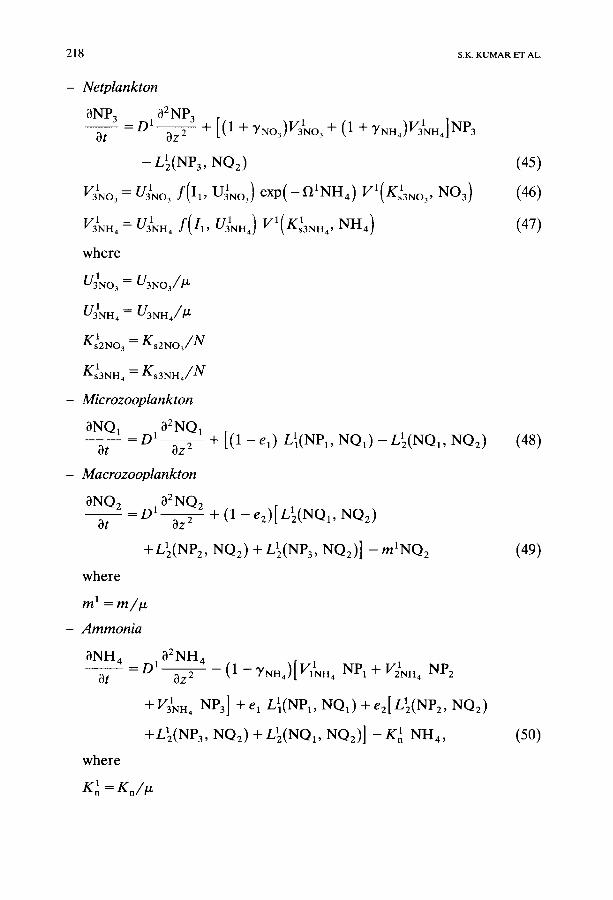
- Picoplankton

ONP 1 32NP1 - O q- [(1-1-]/No3)V1No3"q- (1-q-'YNH4)VINH4]NP1 Ot aZ 2

- LI(NP1, NQ,) (7)

where

VaNO~ = UINO3 V(KslN03, NO3) g( I , UIN03 ) exp(--fl k NH4) (8)

VINH4 = GNH4 V(KslNH4, NH4) g ( I , GNH4 ) (9)

g(I, U ) = [1 - e x p ( - a I / U ) ] e x p ( - I / 5 0 0 ) (10)

N V(Ks, N ) - Ks + N (11)

LI(P, Q ) = / 1 1 1 - exp(-A1P)] Q (12)

I is given by equation (4), a is the slope of the initial linear portion of the g versus I curve (e.g. Platt et al., 1980; Vincent et al., 1989b), and l 1 and A 1 are as explained in equation (3).

- Nanoplankton

ONP 2 O 2 NP 2 0t - - D ~ + [ ( 1 "q-YNO3 ) V2NO3+(1 q"TNH,) V2NH,)]NP2

- L2(NP 2, NQ2) (13)

where

V2NO3 = U:NO3 V(Ks2NO 3, NO3) exp ( - 12 NH4) g ( I , U2NO3) (14)

V2NH4 = U2NH4 V(Ks2NH4, NH4) g(I, U2NrL ) (15)

L2(P, Q)=12[1-exp(-AP)]Q (16)

and l 2 and /~2 a r e as explained in equation (3);

200

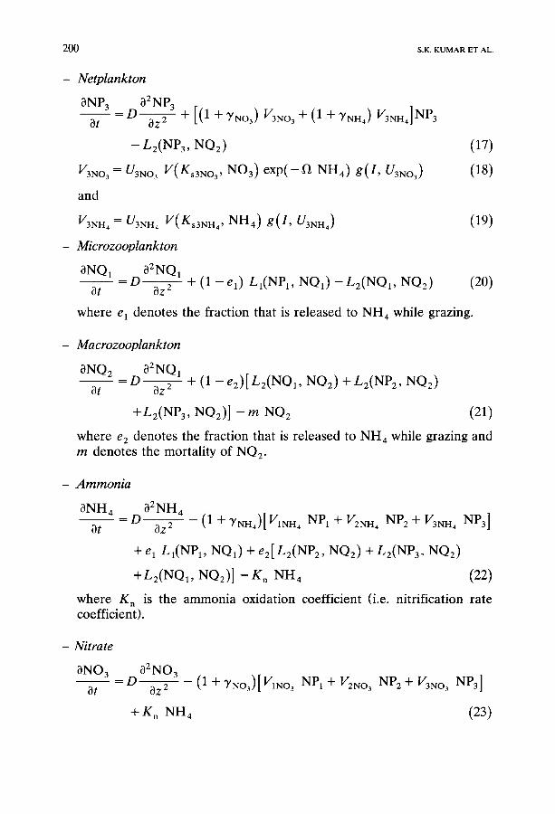
- Netplank ton

S.K. KUMAR ET AL.

3NO

and

V3NH

ONP 3 a2NP3 a~- - D ~--~ 5 - + [(1 +YN%) VaNO~ + (1 + YNH.) VaNH4]NP3

-- L2(NP3, NQ2)

= U3NO3 V(Ks3NO,, N O 3 ) e x p ( - a N H 4 ) g ( I , U3NO3 )

= U3NH4 V(Ks3NH4, N H 4 ) g(I, U3NH4 )

Microzooplankton

0NQ 1 02NQ1 D -

Ot OZ 2

(17)

(18)

(19)

+ (1--el) LI(NP1, NO,) - L2(NQ1, NQ2) (20)

where e 1 denotes the fraction that is released to NH 4 while grazing.

Macrozooplank ton

aNQ 2 a2NQ1 - - - D - - + (1 -eE)[L2(NQ1, NQ2) +L2(NP2, NQ2) at OZ 2

+Lz(NP3, NQ2)] - m NQ2 (21)

where e 2 denotes the fraction that is released to NH 4 while grazing and m denotes the mortality of NQ 2.

- A m m o n i a

0NH 4

0t

a2NH4 - - = D - - (1-4-'YNH4)[V1NH, NPI-t-V2NH4 NP2-t-V3NH, NP3] ~z 2

+ e 1 LI(NP1, NQ1) + e2[L2(NP 2, NQ2) + L2(NP 3, NQ2)

+Lz(NQ 1, NQ2) ] - K n NH 4 (22)

where K n is the ammonia oxidation coefficient (i.e. nitrification rate coefficient).

- Nitrate

~NO 3 02N03 Ot Oz 2

+ K n NH 4

(1 + YNO3)[VaNo~ NP 1 + V2No3 NP 2 + V3NO3 NP3]

(23)

P I C O P L A N K T O N A N D M A R I N E F O O D C H A I N D Y N A M I C S 201

Initial conditions. Since we are dealing with a well-mixed layer all the concentrat ions have uniform concentrat ions initially, i.e.

C ( z , O ) = C o (24)

where C o is a vector independent of z. The values for C o were taken from the field data obtained from the West Coast of the South Island, and were set as concentrations that were recorded immediately after an upwelling event (see Table 2).

Boundary conditions. We assume zero-flux conditions for all the variables at z = 0, the surface of the ocean. At the bot tom of the mixed layer, z = ZL, we assume zero-flux condition for all variables except NO 3. For NO 3 we assume that there is an upward diffusion from beneath the mixed layer. These conditions are mathematically expressed as:

OC - 0 at z = 0

Oz

and

D - - + H ( C - C 1 ) = O at z = z L Oz

where H is a 7 × 7 matrix with elements aii given by:

aij = O for i ~ j ~ < 7

a77 = H 1 (a constant)

and the components of C1 are given by:

C i=O for i = 1 , 2 , . . . , 6

and

C7 = NO~ (a constant)

(25)

(26)

(27)

(28)

(29)

(30)

Non-dimensionalisation. All the state variables are non-dimensionalised by N, the total of concentrat ion of nitrogen in all the components at t -- 0, t ime t by tz, the maximum uptake rate of nutrients, and depth z by z L, the depth of the mixed layer. Details are given in the Appendix.

Computational methodology. Equations (32)-(51) (in the Appendix) were solved by the method of lines using conditions (52)-(54). The method of lines can be described briefly as follows. Equations (32)-(51) are written in the finite difference form in the z-direction. Boundary conditions (53) and (54) are substituted in the finite-difference equations. The resulting equa-

202 S.K. KUMAR ET AL.

tions are solved in time direction as initial value problems with the condition (52). The software for this method is given in NAG (Numerical Analysis Group) Library's section on partial differential equations D03. Numerical experiments showed that to obtain a three-significant-digit accu- racy it was sufficient to discretise in the z-direction with 81 points and with a step size of 0.08 in the time direction.

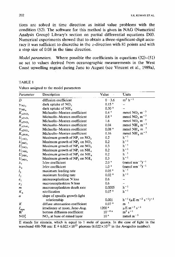
Model parameters. Where possible the coefficients in equations (32)-(51) ae set to values derived from oceanographic measurements in the West Coast upwelling region during June to August (see Vincent et al., 1989a),

T A B L E 1

Values assigned to the model parameters

Parameter Descript ion Value Units

D m 2 h -1

Y NO 3

"~ NH4 KslNO 3 mmol NO 3 m -3 Ks2NO 3 mmol NO 3 m -3 K~3NO 3 mmol NO 3 m -3 K~lNH 4 mmol NH 4 m -3

Ks2NH 4 mmol NH 4 m -3 Ks3NH 4 mmol NH 4 m -3

U1NO3 h - 1

U2N03 h - 1

U3N03 h - 1

U1NH4 h - 1

U2NH4 h -- 1

U3NH4 h - 1 1 (mmo1 n m - 3)- 1

/~ 2 (mmol n m - 3)- 1

l 1 h -1 12 h -1

e 1

e 2 m h -1

Kn h -1

o~

diffusion coefficient 0 - 3.6 dark uptake of NO 3 0.15 a

dark uptake of NH 4 0.30 a

Michae l i s -Men ten coefficient 0.4 a

Michae l i s -Men ten coefficient 0.8 a

Michae l i s -Men ten coefficient 1.6 Michae l i s -Men ten coefficient 0.04 Michae l i s -Men ten coefficient 0.08 a Michae l i s -Men ten coefficient 0.16

Maximum growth of NP 1 on NO 3 0.2 Maximum growth of NP 2 on NO 3 0.2 Maximum growth of NP 3 on NO 3 0.3 Maximum growth of NP 1 on NH 4 0.2 Maximum growth of NP 2 on NH 4 0.2 Maximum growth of NP 3 on NH 4 0.3 Ivlev coefficient 2.0 a

Ivlev coefficient 1.0 a maximum feeding rate 0.05 a maximum feeding rate 0.02 a

microzooplankton N loss 0.6 macrozooplankton N loss 0.6 macrozooplankton death rate 0.0005 nitrification 0.07 a slope of specific growth-light

relat ionship 0.001 h -1 (lxE m -2 s - l ) -1

K diffuse at tenuat ion coefficient 0.07 a m - 1 /max irradiance at noon, June-Aug. 1200 a I~E m -2 s -~ H 1 bot tom diffusion coefficient 10-8 a m 2 s - 1 NO31 NO 3 at base of mixed layer 10 a mmol m -3

E stands for einstein, which is equal to 1 mole of quanta. In the case of light in the waveband 400-700 nm: E ~ 6.022 × 1023 photons (6.022 × 1023 in the Avogadro number) .


the time when the commercially important fish species migrate in to breed. Additional values are derived from Wroblewski (1988) and Moloney et al (1986). the coefficients and their values are listed in Table 1.

R E S U L T S

The model described above was run to simulate the response to an upwelling event which has uniformly diluted the five categories of plankton throughout the water column and has increased the nitrate concentrations to 10 mmol m -3 (Table 2). Concentrations vary with time and depth as determined by the equations of the reaction-diffusion system, in which the diffusion coefficient (D) is set to a range of values over several powers of ten. In the West Coast system there are large variations in the physical environment at timescales of 1 to 4 weeks (Heath, 1986); consequently our simulations extend to 30 days.

Solutions in time. The temporal dynamics at the surface of the water column (z = 0) of each of the nitrogen species is shown in Fig. 2, for a mixed layer depth of 100 m and for D = 3.6 m 2 h -1 (moderate mixing). This figure shows the variation of all the components over 30 days. It can be seen that all the plankton species rise to a peak and then fall: NQ 2 peaks sometime after 30 days. These peaks occur at different times: NP 1 at 5, NP 2 at 25, NP 3 at 20, and NQ 1 at 15 days. One of the consequences of these population offsets is that there is a shift from a picoplankton- dominated community to a nanoplankton-dominated community at

T A B L E 2

Init ial condi t ions for the model led s tate variables

Var iab le Concen t r a t i on (mmol N m -3)

Phy top lank ton NP 1 0.15 NP 2 0.10 NP 3 0.05

Z o o p l a n k t o n N Q a 0.05 N Q 2 0.025

Nut r i en t s N H 4 0.05 N O 3 10.0

Total 10.425

204 S.K. K U M A R ET AL.

t (non-dimensional)

0.00 I 0.00 20.00 30.00 40.00 50.00 0.25 t~,,,,,,r ......... i,,,~l,,, ...... i,,,~JrBl,,,,,,, 1.00

o o i ::: 0.15

N0 3

1 / 0.10 ^

0.00 10.00 20.00 50.00

t ( d a y s )

Fig. 2. Variation of NP 1 (0), NP 2 ( [ ] ) , NP 3 (A) , NQ I (+ ) , NO2 ( * ) , NH4 ( # ) and NO 3 ( e ) with time at the surface of the mixed layer (z = 0) for the diffusion coefficient D = 3.6 m 2 h - 1 and mixed layer depth z e = 100 m. All the ni trogen coefficients are in non-dimensional

form.

timescales of less than 10 days. The net plankton becomes increasingly important with time, but even at its peak is less than 25% of NP 2 concentrations. Both nutrients are consumed by three phytoplankton species that are grazed by the zooplankton which release nutrients. Hence the nutrient trajectories will not settle to steady values until NQ 1 and NQ 2 have settled. These results demonstrate that large transient changes in the distribution of nitrogen between plankton components follow an upwelling event. Steady state is reached in time scales much greater than 30 days.

Changing the diffusion coefficient D results in large variations in the time and depth dependence of all nitrogen constituents. These effects are illustrated in Fig. 3 for NPI, NQa and NO 3 varying with time at z = 0 for three values of D ranging from no mixing (D = 0) to vigorous mixing (D = 360 m 2 h - l ) . Figure 4 shows for the same values of D, the way the concentrations of the same three species, NP1, NQ 1 and NO3, vary with depth, 20 days after an upwelling event. In all these figures, the mixed layer depth has been taken to be 100 meters.


NP 1

0.00 10.00 0 .025 . . . . . . . . . t . . . . ,~, , , , . . . . . . . . .

0

0.020

0 .015

0 .010

0 .005

t (non-dimensional)

20.00 50.00 40.00 50 .00 I I I , I t l l l l J l l t l l , l l l l l l l l l 0.025

0.020

0 . 0 1 5

.0 .010

.0 .005

0 .000 ~ - 0 .000 0 .00 10.00 20 .00 30.00

t (days

t (non dimensional)

0.00 I0.00 20.00 50.00 40.00 50.00 0.025 - ~ - 0 .025

0 .020 -~ / \ ~-- 0 .020

NQ t

0.015 -0 .015

0 .010 q / / ~ - - -"-------~_\ ~ ~--0.010

0 .005 ~ \ } -0 .005

o . o o o ~ o . o o o 0 .00 10.00 20 .00 50.00

t (days)

Fig. 3. Variation of some of the components with time and various diffusion coefficients D = 0 (©), D = 3.6 ( [3) and D = 360 m 2 h -1 (zx) at z = 0 and ZL = 100m. (a) Variations in picoplankton NP 1. (b) Variations in microzooplankton N Q 1. (c) Variation in nitrate N O 3.

2 0 6 S.K. KUMAR ET AL.

NO 3

t (non-dimensional)

0.00 10.00 20.00 50.00 40.00 50.00 1.00 ~: ........ I ......... I ......... I ......... ' ......... I ....... 1.00

0.90 ~ - ~ 0 . 9 0

0.80 - ~ . . 0.80

0.70 ~ - 0.70

060 / 060

O " 5 O ~ . 0.50

0.40 .0.40

0.30 ~ . . . . . . . . . I . . . . . . . . . [ . . . . . . . . . 0*30 0.00 10.00 20.00 50.00

t (days)

Fig. 3 (continued).

In studying Figs. 3 and 4, it is important to recall that the irradiance function determines that the maximum rate of growth of the plankton species occurs a small distance below the surface, at a depth of about 15 m. Consequently after 20 days with D = 0 (no mixing), Fig. 4 shows a maximum in NP 1 and NQ 1 and a minimum in the nutrient NO 3 at z -- 15 m. As D rises to 3.6 m 2 h-1 the diffusive mobility of all these species is sufficient to remove the maximum and the minimum from the trajectories. Unde r conditions of high turbulent diffusion, represent by D = 360 m 2 h -1, the diffusive mobility of each species is sufficient for the water column to be completely mixed in the sense that no concentrat ion profiles exist. Such profiles approximate those measured in the West Coast region (Vincent et al., 1989a).

Figure 4a shows that at 20 days, the NP 1 trajectory for D = 3.6 m 2 h-1, lies above that for D = 0. This results from the different rates of production of NP 1 and its predator up to that time. When snapshots of the NP 1 concentrat ions over depth are taken at different times, the relative posi- tions of the D = 0 and D -- 3.6 m 2 h-1 curves are reversed or, as in Fig. 4b for NQ1, the curves may cross each other. Similar effects characterise the influence of D on the t ime-dependent changes in the nitrogen compo-

P1COPLANKTON A N D M A R I N E F O O D C H A I N D Y N A M I C S

0.0014 q O

2 0 7

0 . 0 0 1 2

0 . 0 0 1 0

NP 1

0 . 0 0 0 8

0 . 0 0 0 5

0 . 0 0 0 4

o

0 . 0 0 0 2

0 . 0 0 0 0 I . . . . . . . . . , . . . . . . . . . , . . . . . . . . . , . . . . . . . . . , . . . . . . . . . ,

0 . 0 0 0 . 2 0 0 . 4 0 0 . 6 0 0 . 8 0 1 .00

NQ 1

0 . 0 1 4

0 . 0 1 3

0 . 0 1 2

0 .011

0 . 0 1 0

0 . 0 0 9

0 . 0 0 8

0 . 0 0 7 , , , , ' ' ' ' , i , . . . . , , , , i , , , , , , , , , i , , , . . . . , , i , , , . . . . , , i 0 . 0 0 0 . 2 0 0 . 4 0 0 . 6 0 0 . 8 0 1 .00

z

Fig . 4. V a r i a t i o n o f s o m e o f t h e c o m p o n e n t s w i t h d e p t h f o r v a r i o u s d i f f u s i o n c o e f f i c i e n t s

D = 0 ( o ) , D = 3 . 6 ( r q ) , a n d D = 3 6 0 m 2 h - 1 ( z x ) a t t h e e n d o f 20 d a y s f o r Z L = 1 0 0 m

( = 1.0 o n t h e n o n - d i m e n s i o n a l d e p t h s c a l e s h o w n ) . ( a ) V a r i a t i o n s in p i c o p l a n k t o n N P 1. ( b )

V a r i a t i o n s in m i c r o z o o p l a n k t o n N Q I. (c ) V a r i a t i o n s in n i t r a t e N O 3.


1 . 0 0 0 0

0 . 9 5 0 0 f

0 . 9 0 0 0

0 . 8 5 0 0

0 . 8 0 0 0

0 . 7 5 0 0

0 . 7 0 0 0

0 . 6 5 0 0

NO 3

o

0 . 6 0 0 0 . . . . . . . . . , . . . . . . . . . , . . . . . . . . . j . . . . . . . . . , . . . . . . . . . 0 . 0 0 0 . 2 0 0 . 4 0 0 . 6 0 0 . 8 0 1 .00

z

Fig. 4 (continued).

nents. At D = 0 there is a recovery in the NP 1 population at t > 25 days resulting from the consumption of NQ1 by NQ 2. This alternation of predator and prey populations is dampened and extended to longer timescales at higher rates of mixing.

Parameter sensitivity. To identify those parameter which the current model is most sensitive to, each of the parameters listed in Table 1 was systemati- cally increased in turn by a factor of ten, while the other parameters were held constant, and the system's behaviour simulated over 30 days. This relatively large incremental factor was chosen after our initial simulations indicated that the incorporation of diffusion substantially lessened the parameter sensitivity of the model. The concentrations of all species at the surface after 5, 10, 20 and 30 days were obtained for each ten-fold parameter increase and the ratio was found of these concentrations to the surface concentrations obtained with initial parameter values.

The results for the most sensitive parameters are shown in Table 3. The ten-fold increase in maximum growth rates (U/No3 and Ulm t , I = 1, 2, 3) and half-saturation constants (Ks/NO 3 and (KstNn,, I = 1, 2, 33 caused less than a ten percent change in the concentrations for any of the nitrogen species. This response to Umo 3 and UINrt 4 is a direct consequence of the


0.00 0 .040

0

0 .035

0.030

0.025

0 .020

0 .015

0 .010

0 .005

50 .00 100.00 150.00 200.00 250.00 300 .00 350 .00 I I I I I I I I I I I I I I I I I I I I I I I t 1 1 1 1 1 1 1 1 1 1 1 1 1 1 1 1 1 1 1 1 1 1 1 1 1 ~ 1 1 1 1 [ 1 1 1 1 [ 1 1 1 1 1 1 1 1 1 1 0.96

/

o ill

0 .96

-0.96

-0.95

-0.95

-0.95

-0.95

-0.95

-0.94

N0 3

0 . 0 0 0 ~ " I . . . . . . . . . . . . . . . . . . . T . . . . . . . . . . . . . . . . . . . 0 . 9 4 0.0~ . . . . . ~'~.~6 . . . . 1%.00 150.00 200.00 250 .6~ ' "%0 .00 350.00

z L 0.00 50.00 100.00 150.00 200 .00 250.00 300 .00 350.00

0.14 t ~3' ' ' ' . . . . ' . . . . . . . . . I . . . . . . . . . ~ . . . . . . . . . ~ . . . . . . . . . I . . . . . . . . . , . . . . . . . . . 0 .96

1 0 . 9 6

0.12 I '0 .95

0 .10 I '0 .95

0.08 I '0.94

0.06 -0.94 NO 3

-0.95

0.04 I -0.93

0.02 I -0.92

0 .00 | . . . . . . . . . ~ . . . . . . . . . ~ . . . . . . . . . ~ . . . . . . . . . ~ . . . . . . . . . ~ . . . . . . . . . ~ . . . . . . . . . 0.92 0 .00 50 .00 100.00 150.00 200.00 250 .00 300 .00 350 .00

z L

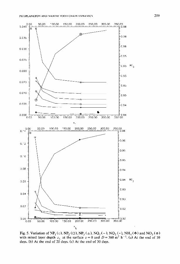
Fig. 5. Variat ion o f N P 1 (©), NP 2 (D), NP 3 (zx), NO1 (+), NO2 (*), NH4 ( O ) and NO 3 ( ~ ) with mixed layer depth z L at the surface z = 0 and D = 360 m 2 h -1. (a) At the end of 10 days. (b) A t the end of 20 days. (c) At the end of 30 days.

210

0.00 0.20 ~ C

0.16

50.00 1.00.00 150.00 200.00 250.00 300.00 350.00 ,-u-q.-- 0.97

0.96

0.96

S.K. KUMAR ET AL.

0.12

0.08

0.95

0.95 NO 3

0.94

0.04

0.94

0.93

0.00 ~ t 0.93 0.00 50.00 100.00 150.00 200.00 250.00 300.00 350.00

z L

Fig. 5 (continued).

form of the terms involving these parameters in equations (32)-(51). We can see this clearly from equation (33), for example. Consider the ratio of VIN03 (with a tenfold increase in U/NO) using initial parameter values. Let us call this ratio f . By expanding f in a Taylor series we find that a tenfold increase in UzNo~ leads only to a small change in f . That is, f ' (0 ) is small, [ f ' (0 ) l << 0.1. In a similar way we can find that it is the same for all other terms involving UINO~ and U/NIJ 4. The model was, however, highly sensitive to changes in the light limitation parameter a and herbivore parameters I i and Ai (i = 1, 2). To a lesser extent the model was sensitive to zooplankton mortality rate m, ammonia oxidation coefficient K n and the light extinction coefficient K (Table 3).

Influence of mixed layer depth. Figure 5 shows how the depth of the mixed layer affects the concentrations of the species present at the surface at 10, 20 and 30 days after an upwelling event. The effect of mixed layer depth on concentrations o f the species present is most marked for mixed layer depths up to 100 m. It is interesting to note that mixed layer depths greater than 100 m have rather little effect at any time on concentrations of the


plankton species or on NH 4 levels, but NO 3 levels rise as the mixed layer is deepened. Such increases in NO 3 levels result from the entrainment of deepwater nutrients and clearly follow from the boundary condition given in equation (54).

DISCUSSION

The simulations described here indicate that large changes can take place in the relative abundance of planktonic nitrogen components within several days of an upwelling event. Our model begins with half of the phytoplankton nitrogen in the picoplankton fraction (NP1). This is in keeping with observations from the West Coast system during high NO3, upwelling conditions (Vincent et al., 1989a). However, a timescales less than ten days, the community shifts towards increasing dominance by the nanoplankton. This is consistent only in part with Cushing's (1989) hypothesis predicting increased proportions of larger-celled plankton under well- mixed, nutrient-rich conditions. In the West Coast ocean the fraction less than 2 p.m rarely drops below 20% of the total winter planktonic biomass (Chang et al., 1989), implying that the patterns simulated here may be continuously disrupted by other processes (e.g. advection) at timescales less than 2 weeks.

The present model is limited by its one-dimensional depiction of the water column. In oceanic systems upwelling is associated with transport across and along the continental shelf, not addressed here. However the model has provided insights into the dynamics of planktonic production and loss subsequent to an episodic nutrient upwelling.

One loss term not incorporated is the sedimentation of NP i and detrital material derived from zooplankton grazing. Sedimentation is likely to have a negligible influence on concentrations of Npl and NP 2 in the mixed layer. For example, Parker (1986) estimates sinking velocities of 0.01 and 0.04 m d-1 for 1 and 2-~m particles, respectively. For a 100-m column this gives sinking time scales greater than 100 days, outside our limits of interest. The absence of a sinking term may however, have resulted in an overestimate of the large-celled NP 3 fraction of the community, and an overestimate of nitrogen recycling from zooplankton grazer (NQ i) activity.

The simulations show a strong effect of macro- and micro-zooplankton grazing on the population size of NP~. This grazing impact restricts the phytoplankton to concentrations less than 0.5 mmol N m-3 over periods of 10 days despite nutrient concentrations that are an order of magnitude higher, and is in keeping with the consistently low winter biomass concentrations observed in the West Coast system (Bradford, 1983).

m.a

TA

BL

E 3

Res

ults

of

the

sens

itiv

ity

anal

ysis

of

mo

st s

igni

fica

nt p

aram

eter

s of

th

e m

od

el a

t th

e su

rfac

e of

th

e m

ixed

lay

er z

= 0

and

Z

L =

100

m

forD

=3

.6m

e

h-1

Inp

ut

Init

ial

valu

e N

P 1

N

P 2

NP

3 N

Q 1

N

Q 2

N

H 4

N

O 3

D

ays

par

amet

er

(dim

ensi

onal

) el

apse

d

m

0.00

05 h

- 1

1.0

1.0

1.0

1.0

0.58

0.

95

1.0

5 0.

95

1.05

1.

06

1.05

0.

34

0.84

1.

0 10

0.

57

1.2

1.3

1.25

0.

13

0.2

0.98

20

0.

13

1.8

2.3

2.43

0.

077

0.1

0.90

30

K n

0.

07 h

- 1

0.9

0.94

0.

97

0.97

1.

0 0.

14

1.0

5 0.

87

0.91

0.

96

0.93

0.

98

0.13

1.

0 10

0.

92

0.86

0.

95

0.94

0.

91

0.14

1.

01

20

0.76

0.

8 0.

98

1.05

0.

81

0.14

1.

03

30

a 0.

001

h-

1 25

.3

16.3

22

.6

28.9

1.

9 6.

1 0.

07

5 (i

tEm

-2

s-l)

-I

K

0.07

m

1

16.3

13

.6

14.5

14

.2

10.5

41

.8

0.01

10

0.

05

2.12

0.

0001

0.

0000

2 77

.6

50.4

0.

04

20

278.

5 0.

0 0.

0 0.

0 19

.7

0.0

0.2

30

0.53

0.

57

0.59

0.

86

0.95

0.

74

1.0

5 0.

38

0.35

0.

39

0.7

0.82

0.

46

1.0

10

0.33

0.

16

0.19

0.

71

0.45

0.

21

1.1

20

0.14

0.

089

0.14

1.

24

0.18

0.

07

1.2

30

12

0.02

h

1 1.

44

0.26

0.

25

0.26

3.

6 2.

02

1.01

5

4.12

0.

013

0.01

27

0.02

3 3.

3 0.

22

1.01

10

68

.1

0.4)

<10

-4

0.4

XlO

4

0.00

12

1.14

0.

005

1.0

20

404.

9 0

.4X

lO

6 0

.5X

10

-6

0

.8x

lO

3 0.

31

0.00

04

0.91

30

I a

0.05

h -

1 0

.6x

10

-5

1.00

1.

0 1.

2 1.

03

0.18

1.

01

5 0.

2 x

10

- lo

0.

964

0.98

0.

75

1.02

0.

27

1.01

10

0

0.94

4 0.

98

0.62

0.

94

0.81

1.

01

20

0 0.

981

1.05

0.

67

0.88

0.

82

1.00

6 30

h~

2.0

(mm

ol

0.1

× 10

3

1.04

1.

03

1.3

1.04

0.

22

1.01

5

nm

-3)

1 0

.3X

lO

9 1.

0 1.

0 0.

8 1.

04

0.3

1.01

10

0.0

0.97

1.

0 0.

65

0.97

0.

82

1.0

20

0.0

0.99

1.

04

0.7

0.92

0.

86

1.0

30

h 2

1.0

(mm

ol

1.32

0.

51

0.40

0.

42

2.97

2.

1 1.

0 5

nm

-3)

-1

3.7

0.05

0.

027

0.04

5 3.

7 0.

63

1.01

10

60

.8

0.7

6x

10

-4

0.4

7x

10

-4

0.1

1×

10

2

1.3

0.5

2×

10

2

1.01

20

36

0.6

0.4

5x

10

-6

0.3

6x

10

-6

0.4

×1

0 -

3 0.

35

0.2

3×

10

3

0.94

30

f~

1.46

2 (m

mo

l 0.

92

0.92

0.

93

0.97

0.

99

0.93

1.

0 5

nm

3

)- 1

0.

91

0.88

0.

89

0.95

0.

97

0.9

1.0

10

0.96

0.

83

0.85

0.

96

0.88

0.

82

1.02

20

0.

8 0.

77

0.85

1.

1 0.

75

0.68

1.

04

30

Th

e en

trie

s in

the

co

lum

ns

un

der

NP1

, N

P2

,...

, N

O 3

are

the

rat

ios

of N

Pj,

NP

2 ..

...

NO

3 w

ith

a te

nfo

ld i

ncre

ase

in a

par

amet

er (

sho

wn

in

colu

mn

2)

to N

P 1,

NP

2,.

..,

NO

3 w

ith

the

no

min

al v

alue

s sh

own

in T

able

1.

214 S.K. K U M A R ET AL.

The strong influence of NQi on NPi biomass is also implied by the sensitivity of the model to the grazing parameters A i and I i (Table 3). This sensitivity analysis also highlights the responsiveness of the system to changes in energy capture by the plankton via the light limitation parameter, a. A similarly high level of sensitivity to changes in a was observed in a more general production model (Vincent et al., 1989b). These results imply that the field programme of oceanographic measurements should pay special attention to accurately quantifying the grazing and light limitation characteristics of the plankton.

The present model has allowed us to gain further insights into the non-linear interactions between light, nutrients and plankton growth under different mixed layer conditions. These results are of special relevance to the West Coast system where large and variable freshwater inflows cause a substantial shallowing of the mixed layer up to 50 nautical miles offshore. This type of model may also be of more general application to oceanographic questions, such as the biological implications of global climate change on the depth of the mixed layer and the influence of inreasing ultraviolet radiation on planktonic food web processes.

Variations in the intensity of mixing, parameterised here in terms of the pseudo-eddy diffusivity value D has major implications for the distribution of organisms down the water column and their temporal dynamics. High D values not only resulted in a homogeneous distribution of nitrogen components through the mixed layer, but also substantially lessened the sensitivity of the model to many parameters (Table 3). At the lowest D values pronounced variations in NP 1 and NQ 1 can developed over relatively short time intervals (e.g. Fig. 4). This level of biological structure is rarely observed in the West Coast system during winter, implying vigorous and frequent mixing of the surface layer.

Mixed layer depth also has a marked effect on the size and Structure of the 5-component plankton community described here. Up to simulation times to 20 days the shallower mixed layers have higher standing stocks of all the plankton components, with greatest effects on the nanoplankton, the nitrogen species showing the fastest net growth. The relationship is non-linear with increasingly large effects at z < 100 m. These results imply an over-riding light limitation on the West Coast phytoplankton population that can be partially relieved by a shallowing of the mixed layer. The effects are likely to be maximal for the time of year simulated: midwinter when surface irradiance is at the annual minimum, and nutrients persist at high concentrations. The simulations, however, clearly establish that the large freshwater inflow to this coastal shelf system can have a major impact on the planktonic biomass and dynamics through its influence on the depth of the surface mixed layer.

P I C O P L A N K T O N A N D M A R I N E F O O D CHAIN D Y N A M I C S 215

ACKNOWLEDGEMENTS

W e t h a n k J. Bradford , R. H e a t h and S. R a h m s t o r f for helpful discus- sions t h r ough the course of this work.

REFERENCES

Andersen, V. and Nival, P., 1988. A pelagic ecosystem model simulating production and sedimentation of biogenic particles: role of salps and copepods, Mar. Ecol. Progr. Set., 44: 37-50.

Andersen, V., Nival, P. and Harris, R.P., 1987. Modelling of a planktonic ecosystem in an enclosed water column. J. Mar. Biol., 67: 407-430.

Bradford, J.M., 1983. Physical and chemical oceanographic observations off Westland, New Zealand. N.Z.J. Mar. Freshwater Res., 17: 71-81.

Chang, F.H., Vincent, W.F. and Woods, P.H., 1989. Nitrogen assimilation by three size fractions of the winter phytoplankton of Westland, New Zealand. N.Z.J. Mar. Freshwa- ter Res., 23: 491-505.

Cushing, D.H., 1989. A difference in structure between ecosystems in strongly stratifierd waters and in those that are only weakly stratified. J. Plankton Res., 11: 1-15.

Dugdale, R.C. and Goering, J.J., 1967. Uptake of new and regenerated forms of nitrogen in primary productivity. Limnol. Oceanogr., 12: 196-206.

Evans, G.T. and Parslow, J.S., 1985. A model of annual plankton cycles. Biol. Oceanogr., 3: 327-347.

Fenchel, T., 1988. Marine plankton food chains. Annu. Rev. Ecol. Syst., 19: 19-38. Frost, B.W., 1987. Grazing control of phytoplankton stock in the open subarctic Pacific

Ocean: a model assessing the role of mesozooplankton, particularly the large calanoid copepods Neocalanus spp. Mar. Ecol. Progr. Ser., 39: 49-68.

Heath, R.A., 1986. One to four weekly currents on the West Coast South Island New Zealand continental slope. Cont. Shelf Res., 5: 645-664.

Iturriaga, R.and Mitchell, B.G., 1986. Chroococoid cyanobacteria: a significant component in the food web dynamics of the open ocean. Mar. Ecol. Progr. Ser., 28: 291-297.

Ivlev, V.S., 1945. The biological productivity of waters. Usp. Sovrem. Biol., 19: 98-120. Moloney, C.L., Bergh, M.O., Field, J.C. and Nevell, R.C., 1980. The effect of sedimentation

and microbial nitrogen regeneration in a plankton community: a simulation investigation. J. Plankton Res., 8: 427-445.

Parker, R.A., 1986. Simulating the development of chlorophyll maxima in the Celtic Sea. Ecol. Modelling, 33: 1-11.

Platt, T., Gallegos, C.L. and Harrison, W.G., 1980. Photoinhibition of photosynthesis in natural assemblages of phytoplankton. J. Mar. Res., 38: 687-701.

Riley, G.A., Stommel, H. and Bumpus, D.F., 1949. Qualitative ecology of the plankton of the Western North Atlantic. Bull. Bingh. Ocean. Collect., 12: 1-169.

Taylor, A.H., 1988. Characteristic properties of models for the vertical distribution of phytoplankton under stratification. Ecol. Modelling, 40: 175-199.

Tett, P., 1981. Modelling phytoplankton production at shelf sea fronts. Phil. Trans. R. Soc. London A, 302: 605-616.

Vincent, W.F., Chang, F.H., Cole, A., James, M.J., Downes, M.T., Moore, M. and Woods, P.H., 1989a. Short term changes in planktonic community structure and nitrogen trans- fers in a coastal upwelling system. Estuarine Coastal Shelf Sci., 29: 131-150.

216 S.K. KUMAR ETAL.

Vincent, W.F., Wake, G.C., Austin, P.C. and Bradford, J.M., 1989b. Modelling the upper limit in oceanic phytoplankton production in the New Zealand exclusive economic zone. N.Z.J. Mar. Freshwater Res., 23: 401-410.

Wroblewski, J.S., 1977. A model of phytoplankton plume formation during variable oregon upwelling. J. Mar. Res., 35: 357-394.

Wroblewski, J.S., Sariments, J.L. and Flierl, G.L., 1988. An ocean basin scale model of plankton dynamics in the North Atlantic: Solutions for the climatogical oceanographic conditions in May. Global Biogeochem. Cycles, 2: 199-218.

APPENDIX

T h e

NP11 = N P I / N

NP~ = N P 2 / N

NP~ = N P 3 / N

N Q ] = N Q I / N

NQ~ = N Q 2 / N

N H ] = N H 4 /N

NO~ = N O 3 / N

t ~ = t/z

non-d imens iona l i s ed s ta te var iables are ca lcu la ted as follows:

(31)

we have:

- Picoplankton

ONP 1 O2Np1 - - _ m _ O 1 - -

at aZ 2 a (1 At- ' ~ N H 4 ) V 1 N H 4 ] N P 1 + [ ( 1 "~-~No3)V1No3"JI - 1

- LI(NPi, NQ,) (32)

V?NO~ = V11~O~ f(I, , VlNO~)exp(-a I NH4) V~(K11NO~, NO~) (33)

V 1 = U 1 V ' ( K 1 N H 4 ) (34) 1N" 4 1N" 4 f ( I 1 , U1NO3) ( slN"4'

f(11, V)= [1 - exp(-alI1)] exp(--lmaxV1/500) a I =alma,,/V (35) N

V l ( K s , N ) - - - (36) K S + N

Z 1 ~--- Z / Z L

w h e r e the superscr ip t '1' indica tes the non-d imens iona l fo rm of the variable. Subst i tu t ing (31) in equa t ions (7) - (23) and d ropp ing the superscr ip ts

PICOPLANKTON AND MARINE FOOD CHAIN DYNAMICS

L (P, Q)=l [1-exp(-al e)]Q 11 = I 1 e x p ( - k l z )

11 = sin[rr(t - 7/x)/(10t,)] for

Io ~ = 0 for

where

D ' = D / ( t x z 2)

UINO = U NO,/ U?NH4 = UINH4/ / .L

K 1 = KsaNo3/N s lNO 3

K 1 = KslNHa//N s lNH 4

l~ = l l / t Z

All = A1N

D, 1 = D . N

- Nanoplankton

ONP 2

0t

V 1 2NO 3

V, 1 2NO 4

L I ( p , Q ) = 1 1 [ 1 - e x p ( - y l p ) ] e

where

7/. < t < 17t,

t<7 /x and t > 1 7 / ,

a2NP2 _ _ 1 (1 + ~NH4)VINH4]NP2 - - 0 1 - + [(1 + ~/No3)V2No3 Jl - OZ 2

- L~z(NP 2, NQ: )

__-- U 1 U 1 N H 4 ) V I [ K 1 N O 3 ) 2NO3 f ( I x ' 2NO3)exp( -~'~1 ~ sNO3,

~-. U 1 U 1 ~ s2NH4, 2NO4 f ( I i , 2NO3 ) V 1[ K' N H 4)

U21NO = UZNO3//z

U I N H 4 = U 2 N H 4 / / £

K 1 = K~2NoJN s2NO 3

K 1 = Ks2NH4/N s2NH 4

l 1 = 12/t,

h I = A 2 N

217

(37)

(38)

(39)

(40)

(41)

(42)

(43)

(44)


N e t p l a n k t o n

0NP 3 02NP3 - - - D ' - - + [(1 + TNo~)V31NO, + (1 + TNH4)V31NHn]NP3 at aZ 2 -

- L~(NP3, NQ2)

K 1 V'13NO3 = U13N03 f(I1, U~N03) e x p ( - f ~ ' N n 4 ) VI( s3NO3, NO3)

V 1 U 1 U 1 K 1

where

U31NO = U3NO/

U I N H 4 = U3NH4/~ ,L

K 1 = Ks2NOj m s2NO 3

K 1 = K s 3 N H a / N s3NH 4

M i c r o z o o p l a n k t o n

aNQ 1 a2NQ1 - - ~ D 1 - -

0t aZ 2

M a c r o z o o p l a n k t o n

aNQ 2 a2NQ2 - - ~ _ _ . O l - -

at az 2

where

+ [(1 - e l ) L](NP1, N Q 1 ) - L~(NQ,, NQ2)

+ (1 - e2) [ L~(NQa, NQ2)

+ L~(NP 2, NQ2) + L~(NP 3, NQ2)] - maNO2

a2NH4 _ _ 1 V) NP 2 - - - - 0 1 ( 1 - ~NH4)[V1NH4 N P 1 + 2NHa 0z 2

+ V31NH, NP3] + e I La(NP1, NO1) + e2[ L~(NP2, NQ2)

+L~(NP 3, NQ2) + L~(NQ1, NQ2) ] - K~ NH4,

m 1 = m / ~

- A m m o n i a

aNH 4 at

where

K 1 = K n / t Z

(45)

(46)

(47)

(48)

(49)

(5o)


- Nitrate

0NO 3 D 1 02NO3 (1 'YNO3)[Vllo3 NP 1 + VINo3 NP2

0t 0z 2

"t- V31NO3 N P 3 ] + g n 1 N H 4

The initial and boundary conditions become:

C( z , O) = C o / N

OC - - = 0 at z = O Oz (Cl) m m zL ~ + ~ c -# o at z = 1

(51)

(52)

(53)

(54)

picoplankton and marine food chain dynamics in a variable mixed-layer

Documents