Ecological Modelling, 51 (1990) 233-250 233 Elsevier Science Publishers B.V., Amsterdam - Printed in The Netherlands

MODELLING THE ENERGY EXCHANGE P R O C E S S E S BETWEEN PLANT COMMUNITIES AND ENVIRONMENT

J IANGUO WU

Botany Department, Miami University, Oxford, OH 45056 (U.S.A.)

(Accepted 17 September 1989)

ABSTRACT

Wu, J., 1990. Modelling the energy exchange processes between plant communities and environment. Ecol. Modelling, 51: 233-250.

A steady-state, one dimensional simulation model based on the gradient diffusion ap- proach is designed to predict the microclimate and properties of energy exchange processes between plant communities and their ambient environment. The architecture of the model is comprised of formulations of turbulent transfer, radiation distribution, and plant community energy balance. The driving forces are meteorological observations above the canopy and the necessary inputs are several geometrical, optical and ecophysiological properties of the community. The model output includes the vertical profiles of radiation, wind velocity, air and leaf temperature, humidity, source strength of heat and water vapor, and total sensible and latent heat fluxes, throughout the community. The results of simulation agree reasonably well with two sets of field measurements reported by other researchers.

INTRODUCTION

Models of energy exchange of plant communities with their environment can help plant ecologists learn more about important interactions among the plant communities, climatic conditions, soils, diseases, and insects (e.g., Waggoner, 1975; Toole et al., 1984). In addition, such models play an important role in modeling the primary production of plant communities. Such models have been developed and applied for different vegetation types (e.g., Waggoner and Reifsnyder, 1968; Stewart and Lemon, 1969; Goudriaan, 1977; Halldin and Lindroth, 1986; Wu, 1987; Wu et al., 1987).

The gradient-diffusion models use flux-gradient profile relationships, adopting a 'first-order' closure approach. Although the gradient-diffusion theory has been well established for the boundary layer above vegetation (Halldin and Lindroth, 1986), the validity of its application within plant communities has been questioned on several grounds (e.g., Legg and

0304-3800/90/$03.50 © 1990 - Elsevier Science Publishers B.V.

234 J. wu

Monteith, 1975; Raupach and Thom, 1981; Meyers, 1985). Nevertheless, the gradient-diffusion approach remains the principal foundation of modeling turbulent transfer processes above and within plant canopies (Halldin and Lindroth, 1986). Models of this sort have provided for "approximate but useful insights into the way in which physical and biological factors combine to govern the transpiration and photosynthesis rates of a plant canopy" (Raupach and Thom, 1981).

The purpose of this study is to develop and test a physically-based, mathematical simulation model of energy exchange processes and microen- vironment of a herb-dominant plant community. Recent improvements in modelling of turbulent transfer processes within canopies have been incor- porated. The model consists mainly of three major components: (a) radia- tion distribution, (b) momentum, heat, and water exchange processes, and (c) energy balance in plant communities.

DESCRIPTION OF THE MODEL *

Radiation distribution in plant communities

Solar radiation transfer. The total shortwave radiation flux density at height z in a plant community is modeled by a simple exponential formula:

ST(Z ) = STC H e x p [ - - a L CLAI(Z)] (1)

where STC H is the solar radiation flux density (W m -E) above the canopy, ot L an empirical extinction constant ranging from 0.3 to 1.5 (Ross, 1975), and CLAI(Z) the downward cumulative leaf area index above height z. CLAI(z) can be related to LAD(Z), leaf area density, by:

CLAI( Z ) = ~ZCHLAD( Z ) d z (2)

where the upper limit of integration ZCH is the average community height.

Longwave radiation transfer. The transfer of longwave radiation in plant communities is modeled through an iterative scheme as Murphy and Knoerr (1972). The total net longwave radiation exchange of a leaf layer at height z with its surroundings are expressed as:

V(z,

+ V(z, GRD) O(TG 4 - TL(Z) 4) + ~-'.V(z, X) O(TL(X) 4 - TL(Z) 4) (3)

* See Appendix.

ENERGY E X C H A N G E PROCESSES BETWEEN PLANT COMMUNITIES A N D ENVIRONMENT 235

where o is the Stefan-Boltzmann constant, TsK the apparent sky tempera- ture, T o the ground surface temperature, and TL(Z ) the mean temperature of leaves in the layer at height z; all temperatures are expressed in kelvin.

Total net radiation. The total absorbed radiation Rr~ is simply the alge- braic sum of absorbed solar radiation Sr~ and absorbed longwave radiation L N within plant communities:

R N ( z ) = S N ( z ) + L N ( z ) (4)

in which absorbed shortwave radiation can be evaluated from:

S N ( z ) = aL S.r(Z ) (5)

where a L is the leaf absorptivity for solar radiation.

Momentum, heat and water vapor exchange processes

Wind profile and momentum transfer. In neutrally stratified atmosphere (i.e., where potential temperature is constant with height and vertical heat flux is zero), the vertical mean wind velocity gradient is:

dU U* d--i - k ( z - d ) for z >_ Zc. (6)

Integrating equation (6) yields:

U* U ( z ) = - - ~ - l n z - d for z > (7) Z--0 - - Z C H

where U(z) is the wind speed (ms -a) at height z above the canopy, k is Von Karman's constant, d is the zero plane displacement height (m), z 0 is the surface roughness length (m), and U* is the friction velocity or eddy velocity with the unit ( m s - l ) .

In unstable conditions (i.e., where temperature decreases with height and there exists an upward heat flux), the vertical transfer processes can be enhanced by buoyancy effect which is inversely dependent on the existing wind shear. In stable conditions (i.e., where temperature increases with height and there exists a downward heat flux), the vertical motions may be retarded somewhat. Apparently the stability of the atmosphere affects the velocity gradients, the entire wind profile, and the vertical transport processes of heat and mass.

With consideration of the buoyant effects, the wind speed gradient above a plant community can be described as:

dU U* d z - k ( z - d ) ~brn(/-') for Z ~___ Z C H (8)

236 J. wt;

and the wind profile can be obtained by integrating (8):

U* [In z2 - d ~m2(F) ..~ ~ml(F )] V(zz ) - V(zm)=--k-[ ~ -d (9)

in which Cm(#) is the stability function for momentum and ~m(F) is the integrated momentum stability parameter. To solve the above equations, specifications of several parameters are required.

d and z 0 are estimated from the equations recommended by Monteith (1975) and Goudriaan (1977):

log d = 0.9793 log ZcI_ I - 0.1536 (10)

and

log z 0 = 0.9970 log Zci_ I - 0.8830 (11)

The friction velocity, U*, is estimated from:

kV(z ) U * = ln[(ZRH--e)/zo]- ~m(FRH) (12)

where subscript (rot) stands for the reference height. The stability functions era(F) for momentum, Ca(F) for heat, and ~w(F)

for water vapor may be expressed as (sensu Dyer, 1974; Brutsaert, 1982):

, , ( r ) -- , w ( r ) = * m ( F ) = 1.0 (neutral) (13)

q,h(e) = q,w(F) = q , L ( F ) = (1 - 16F) -a/2 (unstable) (14)

¢h(F) = q~w(F)= q~m(F)= 1 + 5F (stable) (15)

where F is defined by

z - d F--~- Zm----- ~ (16)

in which Lmo is called Monin-Obukhov length (m), defined as:

Lmo(Z) = _ pCpTA(z) U* kgSH (17)

where 0 is the air density, g is the acceleration of gravity (ms-2) , Cp the specific heat of air (Jkg -1 o C-1), TA(Z ) the air temperature at height z, and sI-I the sensible heat flux density (W m-2).

The wind profile within plant communities is obtained from:

U(z)=U(zcn)exp[aw(Z/Zcrt-1)] for Z<Zcu (18)

where a w is the extinction coefficient.

E N E R G Y E X C H A N G E PROCESSES BETWEEN PLANT C O M M U N I T I E S A N D E N V I R O N M E N T 237

Heat and water vapor transfer. Because of the rather small heat capacity of the air, the transfer process can be treated as a steady state case (i.e., dTg/d t = d Q k / d t = 0). The profiles of air temperature and specific humid- ity between two arbitrary levels z a and z 2 above plant communities can be computed from:

SH [ln z2--d o.(r2)+oh(rl)] TA, = rA2 + p C p k U * / z, - d

and

(19)

K h ( z ) =

and

The eddy diffusivities K h and K w are modeled as (Dyer, 1974; Mehlen- bacher and Whitfield, 1977):

k U * ( z - d ) for Z>zcH (21) Ch

k U * ( z - d ) for Z>ZcH (22) r w ( Z ) = ew

The steady-state vertical fluxes of sensible and latent heat within plant communities may be described by the following differential equations:

dSH pCp ( TL ( Z ) - TA ( Z ) ) LAD( z ) d--T = Rh(z ) (23)

and

dEE PLt(QL(z) - -QA(Z))LAD(z) dz R w ( z ) + R s ( z )

The mean temperature and specific humidity profiles of air and leaves within a plant community can be predicted by solving the two second-order differential equations with specifications of the structural characteristics of the community and the turbulent diffusive properties of its ambient atmo- sphere.

The eddy diffusivity within canopies is modeled after Mehlenbacher and Whitfield (1977)"

Kh(Z ) = Khc H exp(aK(Z/Zcn -- 1) for z < Zc. (25)

where Khc n is the thermal eddy diffusivity at the canopy height, and a K is the extinction coefficient.

(24)

LE [ lnZ2- d Ow(F2) + Ow(F1)] (20) QAa=QA2 + p L t k U * [ z 1 - d

238 s. wu

The leaf boundary resistance is calculated from (Gates, 1980; Paw U and Gueye, 1983):

R h ( z ) = C [ DL 11/2 (26) U(z) l

where D L is the average leaf dimension (m) and C 1 is a constant. Following Mehlenbacher and Whitfield (1977), stomatal resistance profile

is obtained from: /

Rs(z ) = DRy(z ) /146.0

in which

DRy(Z) = Q L ( z ) - Q A ( Z ) Qcrit

D R y ( Z ) = 1

3.6 ) (27) + 4.59 × 1 0 - 4 S T ( Z ) -1- 0.0015

for QL(z) - QA(Z) > Qcnt

for QL(z) - QA(z) < Qcrit

(28)

(29)

where acrit is the lowest value of leaf-air specific humidity gradient affecting stomatal resistance (0.004 and 0.006 kg/kg for two different corn crops in Mehlenbacher and Whitfield's study).

Energy balance in plant communities

Assumed as a one-dimensional, steady-state process, the energy balance within a plant community can be described as

R N = SH + LE + G (30)

The vertical divergence equation of the energy balance can be expressed as :

dR N 2pCp LAD(g) -- (TL(Z) -- TA(Z)) dz Rh(Z )

2pL t LAD(Z ) + R w ( z ) + R s ( z ) (QL(z ) - -QA(z ) ) (31)

The profile of leaf temperature is then obtained by solving the equation:

Rh(z) Lt Rh(z) (QL(Z) -- QA(z)) (32) TL(Z)=TA(Z)+ 2O------~-p R s ( z ) - - Cp(Rw(z )+Rs(z ) )

S I M U L A T I N G S C H E M E OF THE M O D E L

The basic inputs for the simulation are: (a) upper boundary conditions: the radiation, air temperature, specific humidity, and wind speed at the

ENERGY EXCHANGE PROCESSES BETWEEN PLANT COMMUNITIES AND ENVIRONMENT 239

reference height; (b) lower boundary conditions: the temperature and specific humidity at the soil surface; and (c) stand information: the downward cumulative leaf area index or the vertical distribution of leaf area density, the average dimension of leaves, and the average height of the plant community.

The energy balance and microenvironment within a plant community is simulated by finding a unique convergent solution for the system of equa- tions described in the foregoing sections. Certain auxiliary formulations are needed for closing the system. Because the solutions to each of the three subsystems depends on those to the other two, the system of equations has to be solved simultaneously through successive approximations.

BEGIN

II Boundary Conditions II I

I Initialize Leaf Temperature and Humidity Profiles I

[ Calculate Absorbed Solar Radiation and Visible Beam l

I Initialize Stability Parameters for Neutral Conditions l

- - Diabatic Loop >I w

I Find Stability Correction Parameters I I

Calculate Friction Velocity and Wind Speed Profile l l

Calculate Leaf Boundary Layer Resistances I l

Compute Heat Turbulent Diffusivit7 Profile I

I~ - - Adiabatic Loop - -

I Compute Air Temperature and Humidity Profile above Stands l

I Calculate stomatal Resistance of Leaves I l

1 Compute Air Temperature and Humidity Profile in Stands I

I Recompute Leaf Temperature and Specific Humidity Profiles I

I Recompute Lonqwave and Total Radiation Absorbed by Stands I

Calculate Heat and Water Vapor Source Strengths and I Total Sensible and Latent Heat Fluxes form Stands l

--Diabatic~ Check for Convergence of Iteration ~Adiabatic-- Loop -- ~ Loop

Final Output I

Fig. 1 A flow chart of the simulation model (PASSM).

240 J. wv

The simulation model is constructed with two main loops. The loop for neutral conditions (adiabatic loop) is first iterated to convergence. The loop for stable or unstable conditions (diabatic loop) then begins iterating until the unique solution of the system of equations is found (Fig. 1). The convergence test is based upon air temperature. In most cases, only five to

2 1.9 1.8 1.7 1.6 1.5 1.4 1.3 1.2

3:1.1

" ~ 0 . 9

0.8

0.7 0 .6 0 .5 0.4 0.3 0 .2

0.1 0

19

2 m

1.9 1.8 1.7 1.6 1.5 1.4 1.3 1.2

=1.1

~ 0 . 9 •

0 . 8 . 0 . 7 0 .6 0 .5 0 . 4 0.3 0 . 2 0.1

0 0 . 0 0 5

Air temperature profile S-L Corn (12:00 EST, Aug.15,1968)

~ i J i i i i J i

21 23 25 27 29

TA ( C e l s i u s )

Air humidity profile S-L Com 12:00 EST, Aug.15, 1968)

'I 1 . 9

1.8 1.7 1.6 1.5 1.4 1.3 1.2

Z1.1

~ 0 . 9 o-ii 0.7 0 .6 0 .5 0.4 0.3 0 .2 0.

l

18

2 1 . 9

1.8 1.7 1.6 1.5 1.4 1.3 1.2

.1-1.1

0.9

Air temperature profile S-L Corn (12:00 EST, Aug.18,1968)

A 9 - ~ 2 4 2 6 28

TA (Celsius)

Air humidity profile S-L Corn 12:00 EST, Aug.18,1968)

I

o . 0.7 0.6 0.5 0.4 0.3 0.2 0.1

i i i r i i ] i i 0 r J i i i , J i r

0.007 0.009 0.011 0.013 0.015 0.005 0.007 0.009 0.011 0.013 0.015

QA (kg/kg) QA (kg/kg)

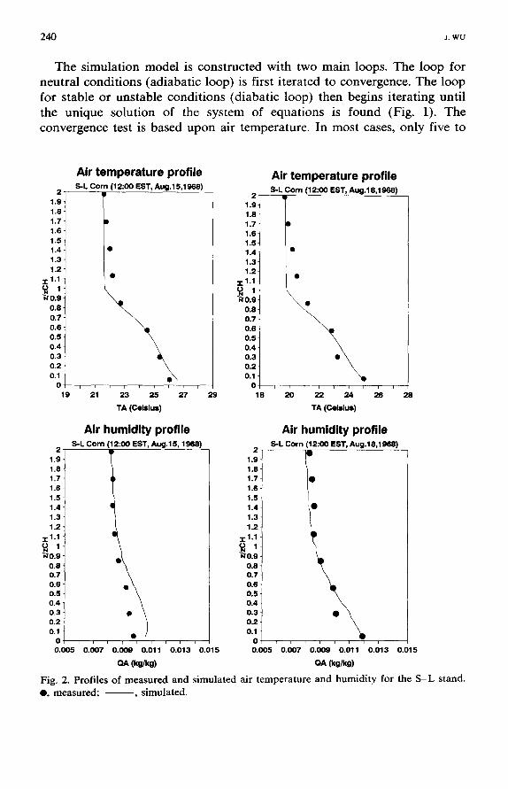
Fig. 2. Profiles of measured and simulated air temperature and humidity for the S-L stand. e, measured; , simulated.

E N E R G Y E X C H A N G E P R O C E S S E S B E T W E E N P L A N T C O M M U N I T I E S A N D E N V I R O N M E N T 241

ten i te ra t ions are needed for e i ther the first or the second convergence to be r eached if the a l lowable d i f fe rence in air t e m p e r a t u r e prof i le be tween two

successive c o m p u t a t i o n s is 0.05 or 0.01 ° C. The c o m p u t e r s imula t ion mode l (PASSM) has been deve loped in F o r t r a n language.

Air tem ;)erature profile Air temperature profile B-C Corn, 09:35 EST, Sept.12, 1962) B-C Corn (12:00 EST, SepL12, 1962) 2 7 _

1.9 1 .g 1.8 1.1t 1.7 1.7 1.6 1.6 1.5 1.5 1.4 1.4 1.3 1.3 1.2 1.2

-1-1.1 1.1

~ 0 . 9 0.9 0 . 8 0.8 0 . 7 ~ 0.7 0.6 0.6 0 . 5 0.5 0 . 4 0.4 0 3 o 3 / . 0 . 2 0 . 2 0.1 0.1

0 ~ 0 , , , , , 14 16 18 20 22 14 16 18 2() 22

TA (Celsius) TA (Celsius)

Air temperature profile Air temperature profile B-C Corn (15:03 EST, Sept.12, 1962) B-C Corn (16:02 EST, Sept.12, 1962)

2 2 - - 1.9 ~ 1 .9 1.8- 1 . 8 1.7- 1 . 7 1.6- 1 . 6 1.5- 1.5 1.4- 1.4- 1.3- 1.3- 1.2- 1.2-

:c 1.1 1.1

~0 .9 0.9 o o I / 0.7 0.7 0.6 0.6 0.5 0.5 0.4 / • 0.4 0.3 0.3 0.2 0.2 0.1 0.1

0 - - , 0 I I I T l I I F i I T

14 16 18 20 22 14 16 18 20 22

TA (Celsius) TA (Celsius)

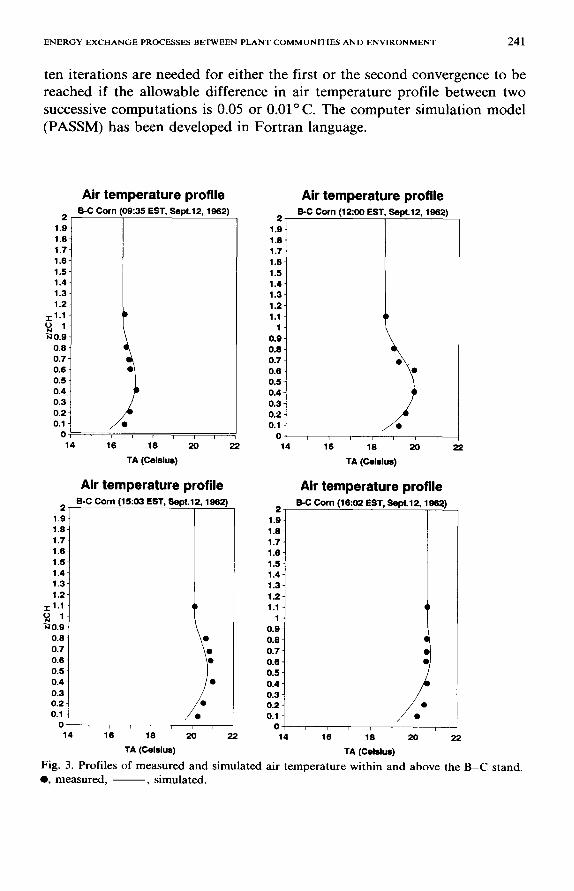
Fig. 3. Profiles of measured and simulated air temperature within and above the B-C stand. e, measured, - - , simulated.

242

S I M U L A T I O N R E S U L T S A N D D I S C U S S I O N

J. W U

The simulation model has been tested with two published sets of field data for corn crops. The first data set contains the measurements by D.W. Stewart and E.R. Lemon and August 15 and 18, 1968 (abbreviated as S-L corn), published by Stewart and Lemon (1969) and Shawcroft et al. (1974). The measurements by K.W. Brown and W. Covey on September 12, 1962 (abbreviated as B-C corn), published by Brown and Covey (1966) and Wright and Brown (1967).

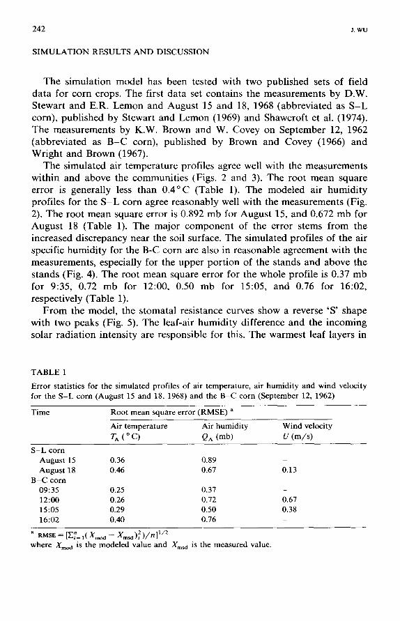
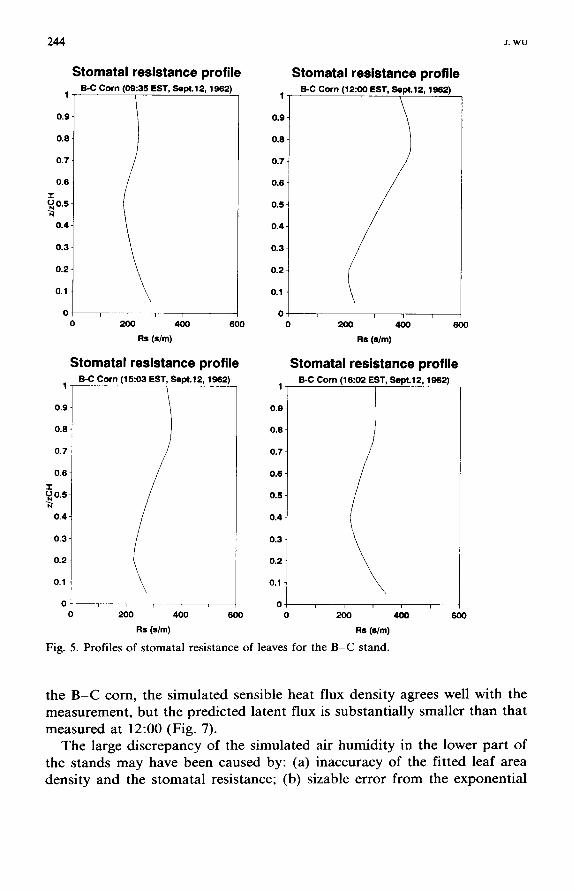
The simulated air temperature profiles agree well with the measurements within and above the communities (Figs. 2 and 3). The root mean square error is generally less than 0.4°C (Table 1). The modeled air humidity profiles for the S-L corn agree reasonably well with the measurements (Fig. 2). The root mean square error is 0.892 mb for August 15, and 0.672 mb for August 18 (Table 1). The major component of the error stems from the increased discrepancy near the soil surface. The simulated profiles of the air specific humidity for the B-C corn are also in reasonable agreement with the measurements, especially for the upper portion of the stands and above the stands (Fig. 4). The root mean square error for the whole profile is 0.37 mb for 9:35, 0.72 mb for 12:00, 0.50 mb for 15:05, and 0.76 for 16:02, respectively (Table 1).

From the model, the stomatal resistance curves show a reverse 'S' shape with two peaks (Fig. 5). The leaf-air humidity difference and the incoming solar radiation intensity are responsible for this. The warmest leaf layers in

T A B L E 1

Error statistics for the s imulated profiles of air temperature , air humidi ty and wind velocity for the S - L corn (August 15 and 18, 1968) and the B - C corn (September 12, 1962)

Time Root mean square error (RMSE) a

Air t empera ture Air humidi ty Wind velocity TA (o C) QA (rob) U ( m / s )

S - L corn Augus t 15 0.36 0.89 - Augus t 18 0.46 0.67 0.13

B - C corn 09:35 0.25 0.37 - 12:00 0.26 0.72 0.67 15:05 0.29 0.50 0.38 16:02 0.40 0.76 -

a valse = [E;'=l(Xmo~ - XmsJ,) / '] 1/2 where Xmo a is the modeled value and Xms d is the measured value.

E N E R G Y E X C H A N G E P R O C E S S E S B E T W E E N P L A N T C O M M U N I T I E S A N D E N V I R O N M E N T 243

Air humidity profile Air humidity profile B-C Corn (09:35 EST, Sept.12, 1962) B-C Corn (12:00 EST, Sept.12, 1962)

21 - ' / 1 . 9 ~ 1.94 1.8 ~ 1.8 4 1.7 i 1.74 1 . 6 ~ 1.64 1.5- 1.54 1.4 - 1.4 1.3 - 1.3 q 1.2 - 1.2

"1" 1.1 1_1 -I

"~ 0.9 0.9 q 0.8 - i l ~ 0.8 -I 0.7 - ~ 0.7 q

0.6 - 0.6 4 0 . 5 - 0 . 5 4

0,4 - e e ~ e 0.44 0.3- 0.34 0.2- 0.24 • 0.1 - 0.1 q •

0 I I I I I [ I 1 | I ~ I I I [ r

10 12 14 18 18 10 12 14 16 18

QA (rob) QA (mb)

Air humidity profile Air humidity profile B-C Corn 15:03 EST, Sept.12, 1962) B-C Corn (16:02 EST, Sept.12, 1962)

2- 1 . 9 - 1 . 8 - 1 . 7 - 1.8 1.5- 1 . 4 - 1.3- 1.2-

~ 0 , 9 0.8- • • 0.7 o.s ! 0.5- 0 . 4 ~ • 0.3 0.2 0.1

0 ~ , , r , , 10 12 14 16 18 10 12 14 16 18

OA (mb) OA (mb) Fig. 4. Profiles of measured and simulated air humidity within and above the B-C stand, e, measured, - - , simulated.

both of the stands appear in the upper part of the communit ies (Fig. 6). The largest leaf-air temperature difference occurs near the canopy top, which is consistent with the observat ion of Brown and Covey (1966).

The measured and simulated sensible and latent heat flux densities for the S - L corn on two different days agree well with the field data (Table 2). For

2 4 4 J. w o

0.9

0.8

0.7

0.6

ON0.5

0.4.

0 . 3

0 . 2

0.1

0 - -

1

0.9-

0 . 8 -

0.7

0 . 6 -

T ~0 .5

0.4

0.3

0.2

0.1

0 0

Stomatal resistance profile B-C Corn (09:35 EST, Sept.12, 1962)

i i i 0 200 400 600

Rs (s/m)

Stomatal resistance profile B-C Corn (15:03 EST, Sept.12, 1962)

i T I 200 400 600

Rs (s/m)

Stomatal resistance profile 1 B-C Corn (12:00 EST, Sept.12, 1962)

0 i 0 6 O O

0 600

0.9

O.fl

0.7

0.6

0.5

0.4

0.3

0.2

0.1

0 .9

0 .8

0.7-

0.6-

0.5-

0.44

o3 t 0.2

0.1 -; I

o l

200 400

Rs (s/m)

Stomatal resistance profile B-C Corn (16:02 EST, Sept.12, 1962)

400 2OO

Rs (s/m)

F i g . 5. P r o f i l e s o f s t o m a t a l r e s i s t a n c e o f l e a v e s f o r t h e B - C s t a n d .

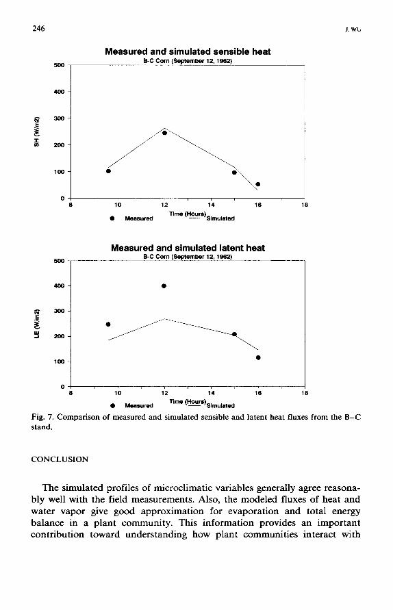
the B-C corn, the simulated sensible heat flux density agrees well with the measurement, but the predicted latent flux is substantially smaller than that measured at 12:00 (Fig. 7).

The large discrepancy of the simulated air humidity in the lower part of the stands may have been caused by: (a) inaccuracy of the fitted leaf area density and the stomatal resistance; (b) sizable error from the exponential

ENERGY EXCHANGE PROCESSES BETWEEN PLANT COMMUNITIES AND ENVIRONMENT 245

Leaf temperature profile B-C Corn (09:35 EST, Sept.12, 1962) 1

1

0.9 / 0.9

0.8- 0 .8

0.7- 0 .7

0.6- 0 .6 1"

0.5- 0 .5

0.4 - O.4"

0.3 0.3-

0.2 B.2-

0.1 3.1 -

0 , 0 l ~ i i i l i l

14 16 18 20 22 24 18

TL (Cslslus)

Leaf temperature profile 1 B-C Corn (15:03 EST, Sept.12, 1962) 1

0 .9 / 0.9-~

0.8- 0 .8

0.7- 0.7'

0.6- 0 .6 1"

0.5- 0 . 5

0.4 - 0.4 -~

0.2 0.2

0.1 O.

0 E i i r ) i i i i - -

18 20 22 24 26 28 16

TL (Celsius)

F i g . 6 . Profiles of leaf temperature for the B-C stand.

Leaf temperature profile B-C Corn (12:00 EST, Sept.12, 1962)

2O 26

TL (Celsius)

Leaf temperature profile B-C Corn (16:02 EST, Sept.12, 1962)

i i i J i i i i i

18 20 22 24

TL (Celsius)

28

26

models for wind, turbulent diffusivity, and solar radiation; and (c) error in the estimated values of the lower boundary layer. The underestimate for the total latent heat flux is possibly related to the magnitude of the turbulent diffusivity, the stomatal resistance, and the aerodynamic resistance of the leaf boundary layer.

246 J. w u

5OO

Measured and simulated sensible heat B-C Corn (September 12, 1962)

E

"r U)

400

300

200

100

0 8 1'0 1~2 1'4 1'6

• Measured Time (HourS)simulated

18

5O0

Measured and simulated latent heat B-C Corn (September 12, 1962)

400

~- 3oo

l U

100

0 i i

8 1'0 1'2 1'4 1'6 18

• Measured Time (HourS)simulated

Fig. 7. Compar ison of measured and simulated sensible and latent heat fluxes from the B - C stand.

C O N C L U S I O N

The simulated profiles of microclimatic variables generally agree reasona- bly well with the field measurements. Also, the modeled fluxes of heat and water vapor give good approximation for evaporation and total energy balance in a plant community. This information provides an important contribution toward understanding how plant communities interact with

ENERGY EXCHANGE PROCESSES BETWEEN PLANT COMMUNITIES AND ENVIRONMENT 2 4 7

TABLE 2

Comparison of measured and simulated sensible and latent beat fluxes from the S -L corn stand (W m - 2)

August15,1968 August18,1968

Measured a SH 369.9 376.5 LE 258.2 279.0 Simulated SH 330.45 342.01 LE 240.18 275.60

a From Stewart and Lemon (1969).

their environment and may be used toward study of the growth, survival, and reproduction of plants.

The impact of differences in turbulent diffusivity on the prediction of microclimatic profiles and total fluxes has been controversial (cf. Mehlen- bacher and Whitfield, 1977; Halldin and Lindroth, 1986). In this study, it seems that the differences in the values of eddy diffusivity may affect the total fluxes of sensible and latent heat fluxes, but it tends to have much smaller impact on the profiles of air temperature and humidity.

Some aspects of the model need further improvement. First, greater accuracy of prediction of total heat and water fluxes from plant communi- ties is needed. This may require a more comprehensive solar radiation model. Second, the discrepancy of prediction of some variables (e.g., air specific humidity) near the soil surface also requires further refinement of the model.

ACKNOWLEDGEMENTS

I am grateful to Dr. K.T. Paw U (University of California, Davis) and Dr. J.L. Vankat (Miami University, Oxford) for their guidance throughout the study. I also wish to express my appreciation for the use of computer facilities at the Department of Land, Air and Water Resources of UC-Davis and the Department of Botany of MU-Oxford.

REFERENCES

Brown, K.W. and Covey, W., 1966. The energy-budget evaluation of the micrometeorological transfer processes within a cornfield. Agric. Meteorol., 3: 73-96.

Brutsaert, W., 1982. Evaporation into the Atmosphere: Theory, History, and Applications. Reidel, Dordrecht, The Netherlands, 299 pp.

2 4 8 J. w u

Dyer, A.J., 1974. A review of flux-profile relationships. Boundary-Layer Meteorol., 7: 363-372.

Gates, D.M., 1980. Biophysical Ecology. Springer, New York, 611 pp. Goudriaan, J., 1977. Crop Micrometeorology: A Simulation Study. Pudoc, Wageningen, The

Netherlands, 249 pp. Halldin, S. and Lindroth, A., 1986. Pine forest microclimate simulation using different

diffusivities. Boundary-Layer Meteorol., 35: 103-123. Legg, B.J. and Monteith, J.L. 1975. Heat and mass transfer in plant canopies. In: D.A. de

Vries and N.H. Afgan (Editors), Heat and Mass Transfer in the Biosphere. Scripta, Washington, DC, pp. 167-186.

Mehlenbacher, L.A. and Whitfield, D.W.A., 1977. Modeling thermal eddy diffusivity at canopy height. Boundary-Layer Meteorol., 12: 153-170.

Meyers, T.P., 1985. A simulation of the canopy microenvironment using higher order closure principles. Ph.D. dissertation, Purdue University, West Lafayette, IN, 153 pp.

Monteith, J.L., 1975. Principles of Environmental Physics. American Elsevier, New York, 241

PP. Murphy, C.E. and Knoerr, K.R., 1972. Modeling the energy balance processes of natural

ecosystems. Eastern Deciduous Forest Biome-IBP Res. Rep. 72-10, Oak Ridge Natioinal Laboratory, Oak Ridge, T N / D u k e University, Durham, NC, 135 pp.

Paw U, K.T. and Gueye, M., 1983. Theoretical and measured evaporation rates from an exposed piche atmograph. Agric. Meteorol., 30" 1-11.

Raupach, M.R. and Thom, A.S., 1981. Turbulence in and above plant canopies. Annu. Rev. Fluid Mech., 13: 97-129.

Ross, J., 1975. Radiative transfer in plant communities. In: J.L. Monteith (Editor), Vegeta- tion and the Atmosphere, I. Academic Press, New York, pp. 13-55.

Shawcroft, R.W., Lemon, E.R., Allen, L.H., Stewart, D.W. and Jensen, S.E., 1974. The soi l -plant-atmosphere model and some of its predictions. Agric. Meteorol., 14: 287-307.

Stewart, D.W. and Lemon, E.R., 1969. The energy budget at the earth's surface: a simulation of net photosynthesis of field corn. Microclim. Invest. Interim Rep. 69-3, USDA, Cornell University, Ithaca, NY, 132 pp..

Toole, J.L., Norman, J.M., Holtzer, T.O. and Perring, T.M., 1984. Simulating Banks Grass mite (Acari: Tetranychidae) population dynamics as a subsystem of a crop canopy-micro- environment model. Environ. Entomol., 13: 329-337.

Waggoner, P.E., 1975. Micrometeorological models. In: J.L. Monteith (Editor), Vegetation and the Atmosphere, I. Academic Press, New York, pp. 205-228.

Waggoner, P.E. and Reifsnyder, W.E., 1968. Simulation of the temperature, humidity and evaporation profiles in a leaf canopy. J. Appl. Meteorol., 7: 400-409.

Wright, J.L. and Brown, K.W., 1967. Comparison of momentum and energy balance methods of computing vertical transfer within a crop. Agron. J., 59: 427-432.

Wu, J., 1987. A simulation model of energy exchange processes and microenvironment of plant communities. M.S. thesis. Miami University, Oxford, OH, 120 pp.

Wu, J., Paw U, K.T. and Vankat, J.L., 1987. A simulation model of energy exchange processes between plant communities and environment. Bull. Ecol. Soc. Am., 68: 453.

ENERGY EXCHANGE PROCESSES BETWEEN PLANT COMMUNITIES AND ENVIRONMENT

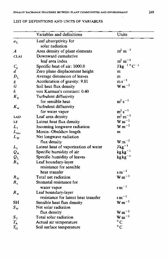
LIST O F D E F I N I T I O N S A N D U N I T S O F V A R I A B L E S

249

Variables and definitions Units

a L Leaf absorptivity for solar radiation

A Area density of plant dements m 2 m-3 C L A I Downward cumulative

leaf area index m 2 m-2 Specific heat of air: 1000.0 Jkg -1 ° C -1 Zero plane displacement height m Average dimension of leaves m Acceleration of gravity: 9.81 m s-1 Soil heat flux density W m-2 yon Karman's constant: 0.40 Turbulent diffusivity

for sensible heat m 2 s-1 Turbulent diffusivity

for water vapor m 2 s-1 Leaf area density m 2 m-3 Latent heat flux density W m-2 Incoming longwave radiation W m - 2 Monin-Obukhov length m Net longwave radiation

flux density W m - 2 Latent heat of vaporization of water J kg-1 Specific humidity of air kg kg- 1 Specific humidity of leaves kg kg-1 Leaf boundary-layer

resistance for sensible heat transfer s m - 1

Total net radiation W m - 2 Stomatal resistance for

water vapor s m - 1 Leaf boundary=layer

resistance for latent heat transfer s m-1 Sensible heat flux density W m-2 Net solar radiation

flux density W m - 2 Total solar radiation W m - 2 Actual air temperature °C Soil surface temperature °C

d D L

g G k Kh

Kw

LAD

LE

L I

Lmo

LN

L t

QA QL Rh

R N

R s

Rw

SH SN

ST

250 J. wv

U U* V

Z 0

ZCH

O~ K

~L

~ W

F

P o

¢ .

Cm Cw #h

Subscripts A CH h L m N RH w

Leaf temperature Apparent sky temperature Wind velocity Friction velocity View factor Vertical distance from

the soil surface Roughness length Average height of a plant community Extinction coefficient for

eddy diffusivity Radiation extinction

coefficient by leaves Extinction coefficient

for wind velocity Stability parameter, defined

by (z - d ) /Lmo Air density Stefan-Boltzmann constant: 5.57 × 10- 8 Stability function for heat Stability function for momentum Stability function for water vapor Integrated stability

parameter for heat Integrated stability

parameter for momentum Integrated stability

parameter for water vapor

A i r

Plant community height Sensible heat Leaf Momentum Net Reference height Water vapor

o C

° C

m s -1 m s -1

m

m

m

k g m -3 W m - 2 K-4