pipelining - upbcsit-sun.pub.ro/resources/cn/comp_arch/chap03.pdf · pipelining is an...
TRANSCRIPT

3
Pipelining 3
It is quite a three-pipe problem.
Sir Arthur Conan DoyleThe Adventures of Sherlock Holmes

3.1 What Is Pipelining? 125
3.2 The Basic Pipeline for DLX 132
3.3 The Major Hurdle of Pipelining—Pipeline Hazards 139
3.4 Data Hazards 146
3.5 Control Hazards 161
3.6 What Makes Pipelining Hard to Implement? 178
3.7 Extending the DLX Pipeline to Handle Multicycle Operations 187
3.8 Crosscutting Issues: Instruction Set Design and Pipelining 199
3.9 Putting It All Together: The MIPS R4000 Pipeline 201
3.10 Fallacies and Pitfalls 209
3.11 Concluding Remarks 211
3.12 Historical Perspective and References 212
Exercises 214
areique
areh stepputer theruc-
t oneould in
s line.
n anall the
Pipelining is an implementation technique whereby multiple instructions overlapped in execution. Today, pipelining is the key implementation technused to make fast CPUs.
A pipeline is like an assembly line. In an automobile assembly line, theremany steps, each contributing something to the construction of the car. Eacoperates in parallel with the other steps, though on a different car. In a compipeline, each step in the pipeline completes a part of an instruction. Likeassembly line, different steps are completing different parts of different insttions in parallel. Each of these steps is called a pipe stage or a pipe segment. Thestages are connected one to the next to form a pipe—instructions enter aend, progress through the stages, and exit at the other end, just as cars wan assembly line.
In an automobile assembly line, throughput is defined as the number of carper hour and is determined by how often a completed car exits the assemblyLikewise, the throughput of an instruction pipeline is determined by how ofteinstruction exits the pipeline. Because the pipe stages are hooked together,
3.1 What Is Pipelining?

126
Chapter 3 Pipelining
e in anown
the pipee time oneave
tage,tep in
ion on
pipe
ore, the.ion.ed as
g theakesuc-a-
ases
thentageis notipe- itsion,ings ofr its thefor-4000ing. the
stages must be ready to proceed at the same time, just as we would requirassembly line. The time required between moving an instruction one step dthe pipeline is a machine cycle. Because all stages proceed at the same time,length of a machine cycle is determined by the time required for the sloweststage, just as in an auto assembly line, the longest step would determine thbetween advancing the line. In a computer, this machine cycle is usuallyclock cycle (sometimes it is two, rarely more), although the clock may hmultiple phases.
The pipeline designer’s goal is to balance the length of each pipeline sjust as the designer of the assembly line tries to balance the time for each sthe process. If the stages are perfectly balanced, then the time per instructthe pipelined machine—assuming ideal conditions—is equal to
Under these conditions, the speedup from pipelining equals the number ofstages, just as an assembly line with n stages can ideally produce cars n times asfast. Usually, however, the stages will not be perfectly balanced; furthermpipelining does involve some overhead. Thus, the time per instruction onpipelined machine will not have its minimum possible value, yet it can be close
Pipelining yields a reduction in the average execution time per instructDepending on what you consider as the base line, the reduction can be viewdecreasing the number of clock cycles per instruction (CPI), as decreasinclock cycle time, or as a combination. If the starting point is a machine that tmultiple clock cycles per instruction, then pipelining is usually viewed as reding the CPI. This is the primary view we will take. If the starting point is a mchine that takes one (long) clock cycle per instruction, then pipelining decrethe clock cycle time.
Pipelining is an implementation technique that exploits parallelism amonginstructions in a sequential instruction stream. It has the substantial advathat, unlike some speedup techniques (see Chapter 8 and Appendix B), it visible to the programmer. In this chapter we will first cover the concept of plining using DLX and a simple version of its pipeline. We use DLX becausesimplicity makes it easy to demonstrate the principles of pipelining. In additto simplify the diagrams we do not include the jump instructions of DLX; addthem does not involve new concepts—only bigger diagrams. The principlepipelining in this chapter apply to more complex instruction sets than DLX oRISC relatives, although the resulting pipelines are more complex. UsingDLX example, we will look at the problems pipelining introduces and the permance attainable under typical situations. Section 3.9 examines the MIPS Rpipeline, which is similar to other recent machines with extensive pipelinChapter 4 looks at more advanced pipelining techniques being used inhighest-performance processors.
Time per instruction on unpipelined machineNumber of pipe stages
------------------------------------------------------------------------------------------------------------
3.1 What Is Pipelining?
127
en-
ple-
reple-inedple-ipe-betro-
these
that thedis-ll the
he
thential
sub-t se-
egis-orary aren the
Before we proceed to basic pipelining, we need to review a simple implemtation of an unpipelined version of DLX.
A Simple Implementation of DLX
To understand how DLX can be pipelined, we need to understand how it is immented without pipelining. This section shows a simple implementation wheevery instruction takes at most five clock cycles. We will extend this basic immentation to a pipelined version, resulting in a much lower CPI. Our unpipelimplementation is not the most economical or the highest-performance immentation without pipelining. Instead, it is designed to lead naturally to a plined implementation. We will indicate where the implementation could improved later in this section. Implementing the instruction set requires the induction of several temporary registers that are not part of the architecture; are introduced in this section to simplify pipelining.
In sections 3.1–3.5 we focus on a pipeline for an integer subset of DLXconsists of load-store word, branch, and integer ALU operations. Later inchapter, we will incorporate the basic floating-point operations. Although we cuss only a subset of DLX, the basic principles can be extended to handle ainstructions.
Every DLX instruction can be implemented in at most five clock cycles. Tfive clock cycles are as follows.
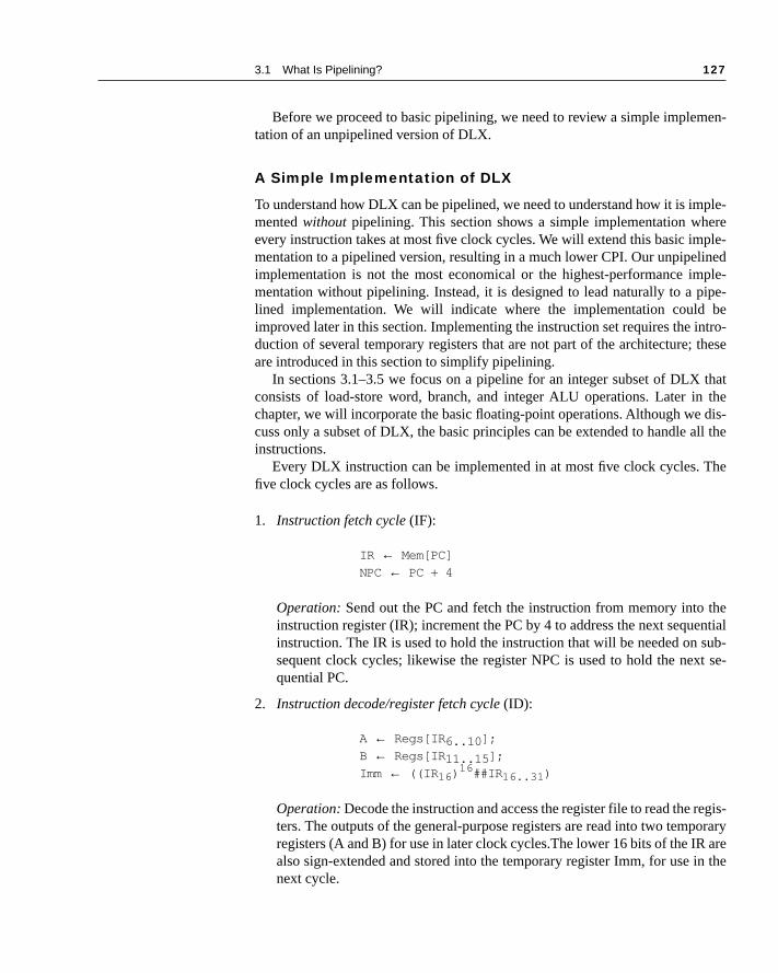
1. Instruction fetch cycle (IF):
IR ← Mem[PC]
NPC ← PC + 4
Operation: Send out the PC and fetch the instruction from memory into instruction register (IR); increment the PC by 4 to address the next sequeinstruction. The IR is used to hold the instruction that will be needed on sequent clock cycles; likewise the register NPC is used to hold the nexquential PC.
2. Instruction decode/register fetch cycle (ID):
A ← Regs[IR 6..10 ];
B ← Regs[IR 11..15 ];
Imm ← ((IR 16) 16##IR 16..31 )
Operation: Decode the instruction and access the register file to read the rters. The outputs of the general-purpose registers are read into two tempregisters (A and B) for use in later clock cycles.The lower 16 bits of the IRalso sign-extended and stored into the temporary register Imm, for use inext cycle.

128
Chapter 3 Pipelining
be-(see
alson ancal-
one
and
ond in
the the
e in beenken.
e
ecu–eeds
Decoding is done in parallel with reading registers, which is possiblecause these fields are at a fixed location in the DLX instruction format Figure 2.21 on page 99). This technique is known as fixed-field decoding.Note that we may read a register we don’t use, which doesn’t help butdoesn’t hurt. Because the immediate portion of an instruction is located iidentical place in every DLX format, the sign-extended immediate is also culated during this cycle in case it is needed in the next cycle.
3. Execution/effective address cycle (EX):
The ALU operates on the operands prepared in the prior cycle, performingof four functions depending on the DLX instruction type.
■ Memory reference:
ALUOutput ← A + Imm;
Operation: The ALU adds the operands to form the effective address places the result into the register ALUOutput.
■ Register-Register ALU instruction:
ALUOutput ← A func B;
Operation: The ALU performs the operation specified by the function codethe value in register A and on the value in register B. The result is placethe temporary register ALUOutput.
■ Register-Immediate ALU instruction:
ALUOutput ← A op Imm;
Operation: The ALU performs the operation specified by the opcode on value in register A and on the value in register Imm. The result is placed intemporary register ALUOutput.
■ Branch:
ALUOutput ← NPC + Imm;
Cond ←(A op 0)
Operation: The ALU adds the NPC to the sign-extended immediate valuImm to compute the address of the branch target. Register A, which hasread in the prior cycle, is checked to determine whether the branch is taThe comparison operation op is the relational operator determined by thbranch opcode; for example, op is “==” for the instruction BEQZ.
The load-store architecture of DLX means that effective address and extion cycles can be combined into a single clock cycle, since no instruction n

3.1 What Is Pipelining?
129
dress,luded
rnsis acasein the
des-
he-g on
d of on aage
to simultaneously calculate a data address, calculate an instruction target adand perform an operation on the data. The other integer instructions not incabove are jumps of various forms, which are similar to branches.
4. Memory access/branch completion cycle (MEM):
The PC is updated for all instructions: PC ← NPC;
■ Memory reference:
LMD ← Mem[ALUOutput] or
Mem[ALUOutput] ← B;
Operation: Access memory if needed. If instruction is a load, data retufrom memory and is placed in the LMD (load memory data) register; if it store, then the data from the B register is written into memory. In either the address used is the one computed during the prior cycle and stored register ALUOutput.
■ Branch:
if (cond) PC ← ALUOutput
Operation: If the instruction branches, the PC is replaced with the branch tination address in the register ALUOutput.
5. Write-back cycle (WB):
■ Register-Register ALU instruction:
Regs[IR 16..20 ] ← ALUOutput;
■ Register-Immediate ALU instruction:
Regs[IR 11..15 ] ← ALUOutput;
■ Load instruction:
Regs[IR 11..15 ] ← LMD;
Operation: Write the result into the register file, whether it comes from tmemory system (which is in LMD) or from the ALU (which is in ALUOutput); the register destination field is also in one of two positions dependinthe function code.
Figure 3.1 shows how an instruction flows through the datapath. At the eneach clock cycle, every value computed during that clock cycle and requiredlater clock cycle (whether for this instruction or the next) is written into a stor

130
Chapter 3 Pipelining
oraryryther
cessive
and12%PI ofbestance
device, which may be memory, a general-purpose register, the PC, or a tempregister (i.e., LMD, Imm, A, B, IR, NPC, ALUOutput, or Cond). The temporaregisters hold values between clock cycles for one instruction, while the ostorage elements are visible parts of the state and hold values between sucinstructions.
In this implementation, branch and store instructions require four cyclesall other instructions require five cycles. Assuming the branch frequency of and a store frequency of 5% from the last chapter, this leads to an overall C4.83. This implementation, however, is not optimal either in achieving the performance or in using the minimal amount of hardware given the perform
FIGURE 3.1 The implementation of the DLX datapath allows every instruction to be executed in four or five clockcycles. Although the PC is shown in the portion of the datapath that is used in instruction fetch and the registers are shownin the portion of the datapath that is used in instruction decode/register fetch, both of these functional units are read as wellas written by an instruction. Although we show these functional units in the cycle corresponding to where they are read, thePC is written during the memory access clock cycle and the registers are written during the write back clock cycle. In bothcases, the writes in later pipe stages are indicated by the multiplexer output (in memory access or write back) that carries avalue back to the PC or registers. These backward-flowing signals introduce much of the complexity of pipelining, and wewill look at them more carefully in the next few sections.
Instruction fetchInstruction decode/
register fetch
Execute/address
calculation
Memoryaccess
Writeback
B
PC
4
ALU
16 32
Add
Datamemory
Registers
Signextend
Instructionmemory
Mux
Mux
Mux
Mux
Zero?Branch
takenCond
NPC
lmm
ALUoutput
IRA
LMD

3.1 What Is Pipelining?
131
tinging we im-ts towouldl to
is re-espe-ly
n isple-
mentoretruc-
nciesere
s andouldike- data
n as im-
ould clockwould in-atae formesd to im-veryount
Sec-nitsgle-
ycle
level. The CPI could be improved without affecting the clock rate by compleALU instructions during the MEM cycle, since those instructions are idle durthat cycle. Assuming ALU instructions occupy 47% of the instruction mix, asmeasured in Chapter 2, this improvement would lead to a CPI of 4.35, or anprovement of 4.82/4.35 = 1.1. Beyond this simple change, any other attempdecrease the CPI may increase the clock cycle time, since such changes need to put more activity into a clock cycle. Of course, it may still be beneficiatrade an increase in the clock cycle time for a decrease in the CPI, but thquires a detailed analysis and is unlikely to produce large improvements, cially if the initial distribution of work among the clock cycles is reasonabbalanced.
Although all machines today are pipelined, this multicycle implementatioa reasonable approximation of how most machines would have been immented in earlier times. A simple finite-state machine could be used to implethe control following the five-cycle structure shown above. For a much mcomplex machine, microcode control could be used. In either event, an instion sequence like that above would determine the structure of the control.
In addition to these CPI improvements, there are some hardware redundathat could be eliminated in this multicycle implementation. For example, thare two ALUs: one to increment the PC and one used for effective addresALU computation. Since they are not needed on the same clock cycle, we cmerge them by adding additional multiplexers and sharing the same ALU. Lwise, instructions and data could be stored in the same memory, since theand instruction accesses happen on different clock cycles.
Rather than optimize this simple implementation, we will leave the desigit is in Figure 3.1, since this provides us with a better base for the pipelinedplementation.
As an alternative to the multicycle design discussed in this section, we calso have implemented the machine so that every instruction takes one longcycle. In such cases, the temporary registers would be deleted, since there not be any communication across clock cycles within an instruction. Everystruction would execute in one long clock cycle, writing the result into the dmemory, registers, or PC at the end of the clock cycle. The CPI would be onsuch a machine. However, the clock cycle would be roughly equal to five tithe clock cycle of the multicycle machine, since every instruction would neetraverse all the functional units. Designers would never use this single-cycleplementation for two reasons. First, a single-cycle implementation would be inefficient for most machines that have a reasonable variation among the amof work, and hence in the clock cycle time, needed for different instructions. ond, a single-cycle implementation requires the duplication of functional uthat could be shared in a multicycle implementation. Nonetheless, this sincycle datapath allows us to illustrate how pipelining can improve the clock ctime, as opposed to the CPI, of a machine.

132
Chapter 3 Pipelining
ting aof the
typi-lock in-
leLX
f the the can-
tion at pipe-ruc-lifiedajor
utionser-
uctionruc- elimi-etch
We can pipeline the datapath of Figure 3.1 with almost no changes by starnew instruction on each clock cycle. (See why we chose that design!) Each clock cycles from the previous section becomes a pipe stage: a cycle in the pipe-line. This results in the execution pattern shown in Figure 3.2, which is the cal way a pipeline structure is drawn. While each instruction takes five ccycles to complete, during each clock cycle the hardware will initiate a newstruction and will be executing some part of the five different instructions.
Your instinct is right if you find it hard to believe that pipelining is as simpas this, because it’s not. In this and the following sections, we will make our Dpipeline “real” by dealing with problems that pipelining introduces.
To begin with, we have to determine what happens on every clock cycle omachine and make sure we don’t try to perform two different operations withsame datapath resource on the same clock cycle. For example, a single ALUnot be asked to compute an effective address and perform a subtract operathe same time. Thus, we must ensure that the overlap of instructions in theline cannot cause such a conflict. Fortunately, the simplicity of the DLX insttion set makes resource evaluation relatively easy. Figure 3.3 shows a simpversion of the DLX datapath drawn in pipeline fashion. As you can see, the mfunctional units are used in different cycles and hence overlapping the execof multiple instructions introduces relatively few conflicts. There are three obvations on which this fact rests.
First, the basic datapath of the last section already used separate instrand data memories, which we would typically implement with separate insttion and data caches (discussed in Chapter 5). The use of separate cachesnates a conflict for a single memory that would arise between instruction f
3.2 The Basic Pipeline for DLX
Clock number
Instruction number 1 2 3 4 5 6 7 8 9
Instruction i IF ID EX MEM WB
Instruction i + 1 IF ID EX MEM WB
Instruction i + 2 IF ID EX MEM WB
Instruction i + 3 IF ID EX MEM WB
Instruction i + 4 IF ID EX MEM WB
FIGURE 3.2 Simple DLX pipeline. On each clock cycle, another instruction is fetched and begins its five-cycle execution.If an instruction is started every clock cycle, the performance will be up to five times that of a machine that is not pipelined.The names for the stages in the pipeline are the same as those used for the cycles in the implementation on pages 127–129: IF = instruction fetch, ID = instruction decode, EX = execution, MEM = memory access, and WB = write back.
3.2 The Basic Pipeline for DLX
133
cycleliver
d for two everynore
verydone
rises
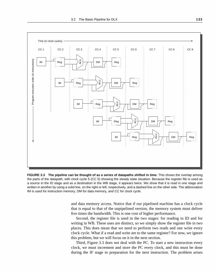
and data memory access. Notice that if our pipelined machine has a clock that is equal to that of the unpipelined version, the memory system must defive times the bandwidth. This is one cost of higher performance.
Second, the register file is used in the two stages: for reading in ID anwriting in WB. These uses are distinct, so we simply show the register file inplaces. This does mean that we need to perform two reads and one writeclock cycle. What if a read and write are to the same register? For now, we igthis problem, but we will focus on it in the next section.
Third, Figure 3.3 does not deal with the PC. To start a new instruction eclock, we must increment and store the PC every clock, and this must be during the IF stage in preparation for the next instruction. The problem a
FIGURE 3.3 The pipeline can be thought of as a series of datapaths shifted in time. This shows the overlap amongthe parts of the datapath, with clock cycle 5 (CC 5) showing the steady state situation. Because the register file is used asa source in the ID stage and as a destination in the WB stage, it appears twice. We show that it is read in one stage andwritten in another by using a solid line, on the right or left, respectively, and a dashed line on the other side. The abbreviationIM is used for instruction memory, DM for data memory, and CC for clock cycle.
ALU
ALU
RegRegIM DM
RegIM DM
Time (in clock cycles)
CC 1 CC 2 CC 3 CC 4 CC 5 CC 6 CC 7
Pro
gram
exe
cutio
n or
der
(in in
stru
ctio
ns)
Reg
CC 8 CC 9
RegIM DM RegALU
RegIM DM RegALU
RegIM DM RegALU

134
Chapter 3 Pipelining
t untilath, ourC orm inre in
in ationss thatisters.
areo thatar.
when we consider the effect of branches, which changes the PC also, but nothe MEM stage. This is not a problem in our multicycle, unpipelined datapsince the PC is written once in the MEM stage. For now, we will organizepipelined datapath to write the PC in IF and write either the incremented Pthe value of the branch target of an earlier branch. This introduces a problehow branches are handled that we will explain in the next section and explodetail in section 3.5.
Because every pipe stage is active on every clock cycle, all operationspipe stage must complete in one clock cycle and any combination of operamust be able to occur at once. Furthermore, pipelining the datapath requirevalues passed from one pipe stage to the next must be placed in regFigure 3.4 shows the DLX pipeline with the appropriate registers, called pipelineregisters or pipeline latches, between each pipeline stage. The registers labeled with the names of the stages they connect. Figure 3.4 is drawn sconnections through the pipeline registers from one stage to another are cle
FIGURE 3.4 The datapath is pipelined by adding a set of registers, one between each pair of pipe stages. The reg-isters serve to convey values and control information from one stage to the next. We can also think of the PC as a pipelineregister, which sits before the IF stage of the pipeline, leading to one pipeline register for each pipe stage. Recall that thePC is an edge-triggered register written at the end of the clock cycle; hence there is no race condition in writing the PC. Theselection multiplexer for the PC has been moved so that the PC is written in exactly one stage (IF). If we didn’t move it, therewould be a conflict when a branch occurred, since two instructions would try to write different values into the PC. Most ofthe datapaths flow from left to right, which is from earlier in time to later. The paths flowing from right to left (which carry theregister write-back information and PC information on a branch) introduce complications into our pipeline, which we willspend much of this chapter overcoming.
Datamemory
ALU
Signextend
PC
Instructionmemory
ADD
IF/ID
4
ID/EX EX/MEM MEM/WB
IR6..10
MEM/WB.IR
Mux
Mux
Mux
IR11..15
Registers
Branchtaken
IR
16 32
Mux
Zero?

3.2 The Basic Pipeline for DLX 135
clesf the
theycontrol mustntil it
n our com-ad orom therrent-m
ere-elineining. Fig- showt twondenttivity the PCsaid dealurce
trols iny theerr theion.ncre-riteheis addi-ce isisterster-lti-cify
All of the registers needed to hold values temporarily between clock cywithin one instruction are subsumed into these pipeline registers. The fields oinstruction register (IR), which is part of the IF/ID register, are labeled when are used to supply register names. The pipeline registers carry both data and from one pipeline stage to the next. Any value needed on a later pipeline stagebe placed in such a register and copied from one pipeline register to the next, uis no longer needed. If we tried to just use the temporary registers we had iearlier unpipelined datapath, values could be overwritten before all uses werepleted. For example, the field of a register operand used for a write on a loALU operation is supplied from the MEM/WB pipeline register rather than frthe IF/ID register. This is because we want a load or ALU operation to writeregister designated by that operation, not the register field of the instruction culy transitioning from IF to ID! This destination register field is simply copied froone pipeline register to the next, until it is needed during the WB stage.
Any instruction is active in exactly one stage of the pipeline at a time; thfore, any actions taken on behalf of an instruction occur between a pair of pipregisters. Thus, we can also look at the activities of the pipeline by examwhat has to happen on any pipeline stage depending on the instruction typeure 3.5 shows this view. Fields of the pipeline registers are named so as tothe flow of data from one stage to the next. Notice that the actions in the firsstages are independent of the current instruction type; they must be indepebecause the instruction is not decoded until the end of the ID stage. The IF acdepends on whether the instruction in EX/MEM is a taken branch. If so, thenbranch target address of the branch instruction in EX/MEM is written into theat the end of IF; otherwise the incremented PC will be written back. (As we earlier, this effect of branches leads to complications in the pipeline that wewith in the next few sections.) The fixed-position encoding of the register sooperands is critical to allowing the registers to be fetched during ID.
To control this simple pipeline we need only determine how to set the confor the four multiplexers in the datapath of Figure 3.4. The two multiplexerthe ALU stage are set depending on the instruction type, which is dictated bIR field of the ID/EX register. The top ALU input multiplexer is set by wheththe instruction is a branch or not, and the bottom multiplexer is set by whetheinstruction is a register-register ALU operation or any other type of operatThe multiplexer in the IF stage chooses whether to use the value of the imented PC or the value of the EX/MEM.ALUOutput (the branch target) to winto the PC. This multiplexer is controlled by the field EX/MEM.cond. Tfourth multiplexer is controlled by whether the instruction in the WB stage load or a ALU operation. In addition to these four multiplexers, there is one ational multiplexer needed that is not drawn in Figure 3.4, but whose existenclear from looking at the WB stage of an ALU operation. The destination regfield is in one of two different places depending on the instruction type (regiregister ALU versus either ALU immediate or load). Thus, we will need a muplexer to choose the correct portion of the IR in the MEM/WB register to spethe register destination field, assuming the instruction writes a register.

136 Chapter 3 Pipelining
ionsindi-achtruc-ution
Basic Performance Issues in Pipelining
Pipelining increases the CPU instruction throughput—the number of instructcompleted per unit of time—but it does not reduce the execution time of an vidual instruction. In fact, it usually slightly increases the execution time of einstruction due to overhead in the control of the pipeline. The increase in instion throughput means that a program runs faster and has lower total exectime, even though no single instruction runs faster!
Stage Any instruction
IF IF/ID.IR ← Mem[PC]; IF/ID.NPC,PC ← (if ((EX/MEM.opcode == branch) & EX/MEM.cond){EX/MEM.ALUOutput} else {PC+4});
ID ID/EX.A ← Regs[IF/ID.IR 6..10 ]; ID/EX.B ← Regs[IF/ID.IR 11..15 ];
ID/EX.NPC ← IF/ID.NPC; ID/EX.IR ← IF/ID.IR;
ID/EX.Imm ← (IF/ID.IR 16) 16##IF/ID.IR 16..31 ;
ALU instruction Load or store instruction Branch instruction
EX EX/MEM.IR ← ID/EX.IR;EX/MEM.ALUOutput ←ID/EX.A func ID/EX.B;orEX/MEM.ALUOutput ← ID/EX.A op ID/EX.Imm;EX/MEM.cond ← 0;
EX/MEM.IR← ID/EX.IREX/MEM.ALUOutput ← ID/EX.A + ID/EX.Imm;
EX/MEM.cond ← 0; EX/MEM.B← ID/EX.B;
EX/MEM.ALUOutput ← ID/EX.NPC+ID/EX.Imm;
EX/MEM.cond ← (ID/EX.A op 0);
MEM MEM/WB.IR ← EX/MEM.IR;MEM/WB.ALUOutput ← EX/MEM.ALUOutput;
MEM/WB.IR ← EX/MEM.IR;MEM/WB.LMD ← Mem[EX/MEM.ALUOutput]; or Mem[EX/MEM.ALUOutput] ← EX/MEM.B;
WB Regs[MEM/WB.IR 16..20 ] ← MEM/WB.ALUOutput;or Regs[MEM/WB.IR 11..15 ] ← MEM/WB.ALUOutput;
For load only:Regs[MEM/WB.IR 11..15 ] ← MEM/WB.LMD;
FIGURE 3.5 Events on every pipe stage of the DLX pipeline. Let’s review the actions in the stages that are specific tothe pipeline organization. In IF, in addition to fetching the instruction and computing the new PC, we store the incrementedPC both into the PC and into a pipeline register (NPC) for later use in computing the branch target address. This structureis the same as the organization in Figure 3.4, where the PC is updated in IF from one or two sources. In ID, we fetch theregisters, extend the sign of the lower 16 bits of the IR, and pass along the IR and NPC. During EX, we perform an ALUoperation or an address calculation; we pass along the IR and the B register (if the instruction is a store). We also set thevalue of cond to 1 if the instruction is a taken branch. During the MEM phase, we cycle the memory, write the PC if needed,and pass along values needed in the final pipe stage. Finally, during WB, we update the register field from either the ALUoutput or the loaded value. For simplicity we always pass the entire IR from one stage to the next, though as an instructionproceeds down the pipeline, less and less of the IR is needed.
3.2 The Basic Pipeline for DLX 137
s lim-ddi-
ce pipeeeded
on oftime,l thatkew,ters,s asng is
lockpathly re- thegle-
The fact that the execution time of each instruction does not decrease putits on the practical depth of a pipeline, as we will see in the next section. In ation to limitations arising from pipeline latency, limits arise from imbalanamong the pipe stages and from pipelining overhead. Imbalance among thestages reduces performance since the clock can run no faster than the time nfor the slowest pipeline stage. Pipeline overhead arises from the combinatipipeline register delay and clock skew. The pipeline registers add setup which is the time that a register input must be stable before the clock signatriggers a write occurs, plus propagation delay to the clock cycle. Clock swhich is maximum delay between when the clock arrives at any two regisalso contributes to the lower limit on the clock cycle. Once the clock cycle ismall as the sum of the clock skew and latch overhead, no further pipeliniuseful, since there is no time left in the cycle for useful work.
E X A M P L E Consider the unpipelined machine in the previous section. Assume that it has 10-ns clock cycles and that it uses four cycles for ALU operations and branches and five cycles for memory operations. Assume that the relative frequencies of these operations are 40%, 20%, and 40%, respectively. Suppose that due to clock skew and setup, pipelining the machine adds 1 ns of overhead to the clock. Ignoring any latency impact, how much speedup in the instruction execution rate will we gain from a pipeline?
A N S W E R The average instruction execution time on the unpipelined machine is
In the pipelined implementation, the clock must run at the speed of the slowest stage plus overhead, which will be 10 + 1 or 11 ns; this is the av-erage instruction execution time. Thus, the speedup from pipelining is
The 1-ns overhead essentially establishes a limit on the effectiveness of pipelining. If the overhead is not affected by changes in the clock cycle, Amdahl's Law tells us that the overhead limits the speedup. ■
Alternatively, if our base machine already has a CPI of 1 (with a longer ccycle), then pipelining will enable us to have a shorter clock cycle. The dataof the previous section can be made into a single-cycle datapath by simpmoving the latches and letting the data flow from one cycle of execution tonext. How would the speedup of the pipelined version compare to the sincycle machine?
Average instruction execution time Clock cycle Average CPI×=
10 ns 40% 20%+( ) 4 40% 5×+×( )×=
10 ns 4.4×=
44 ns=
Speedup from pipeliningAverage instruction time unpipelinedAverage instruction time pipelined
-----------------------------------------------------------------------------------------=
44 ns11 ns------------- 4 times==
138 Chapter 3 Pipelining
n thessiblertiesen-
t two- theing
n bee wille in-
er theis isoint real
E X A M P L E Assume that the times required for the five functional units, which operate in each of the five cycles, are as follows: 10 ns, 8 ns, 10 ns, 10 ns, and 7 ns. Assume that pipelining adds 1 ns of overhead. Find the speedup ver-sus the single-cycle datapath.
A N S W E R Since the unpipelined machine executes all instructions in a single clock cycle, its average time per instruction is simply the clock cycle time. The clock cycle time is equal to the sum of the times for each step in the exe-cution:
The clock cycle time on the pipelined machine must be the largest time for any stage in the pipeline (10 ns) plus the overhead of 1 ns, for a total of 11 ns. Since the CPI is 1, this yields an average instruction execution time of 11 ns. Thus,
Pipelining can be thought of as improving the CPI, which is what we typi-cally do, as increasing the clock rate—especially compared to another pipelined machine, or sometimes as doing both. ■
Because the latches in a pipelined design can have a significant impact oclock speed, designers have looked for latches that permit the highest poclock rate. The Earle latch (invented by J. G. Earle [1965]) has three propethat make it especially useful in pipelined machines. First, it is relatively inssitive to clock skew. Second, the delay through the latch is always a constangate delay, avoiding the introduction of skew in the data passing throughlatch. Finally, two levels of logic can be performed in the latch without increasthe latch delay time. This means that two levels of logic in the pipeline caoverlapped with the latch, so the overhead from the latch can be hidden. Wnot be analyzing the pipeline designs in this chapter at this level of detail. Thterested reader should see Kunkel and Smith [1986].
The pipeline we now have for DLX would function just fine for integinstructions if every instruction were independent of every other instruction inpipeline. In reality, instructions in the pipeline can depend on one another; ththe topic of the next section. The complications that arise in the floating-ppipeline will be treated in section 3.7, and section 3.9 will look at a completepipeline.
Average instruction execution time 10 8 10 10 7+ + + +=
45 ns=
Speedup from pipeliningAverage instruction time unpipelinedAverage instruction time pipelined
-----------------------------------------------------------------------------------------=
45 ns11 ns------------- 4.1 times==

3.3 The Major Hurdle of Pipelining—Pipeline Hazards 139
-s re-e are
notped
ious the
ns
miss. sim-truc-
r thetionsthe
wiseg theche
tionntage willtallingate in
ance.ing,
There are situations, called hazards, that prevent the next instruction in the instruction stream from executing during its designated clock cycle. Hazardduce the performance from the ideal speedup gained by pipelining. Therthree classes of hazards:
1. Structural hazards arise from resource conflicts when the hardware cansupport all possible combinations of instructions in simultaneous overlapexecution.
2. Data hazards arise when an instruction depends on the results of a previnstruction in a way that is exposed by the overlapping of instructions inpipeline.
3. Control hazards arise from the pipelining of branches and other instructiothat change the PC.
Hazards in pipelines can make it necessary to stall the pipeline. In Chapter 1,we mentioned that the processor could stall on an event such as a cacheStalls arising from hazards in pipelined machines are more complex than theple stall for a cache miss. Eliminating a hazard often requires that some instions in the pipeline be allowed to proceed while others are delayed. Fopipelines we discuss in this chapter, when an instruction is stalled, all instrucissued later than the stalled instruction—and hence not as far along in pipeline—are also stalled. Instructions issued earlier than the stalled instruc-tion—and hence farther along in the pipeline—must continue, since otherthe hazard will never clear. As a result, no new instructions are fetched durinstall. In contrast to this process of stalling only a portion of the pipeline, a camiss stalls all the instructions in the pipeline both before and after the instruccausing the miss. (For the simple pipelines of this chapter there is no advain selecting stalling instructions on a cache miss, but in future chapters weexamine pipelines and caches that reduce cache miss costs by selectively son a cache miss.) We will see several examples of how pipeline stalls operthis section—don’t worry, they aren’t as complex as they might sound!
Performance of Pipelines with Stalls
A stall causes the pipeline performance to degrade from the ideal performLet’s look at a simple equation for finding the actual speedup from pipelinstarting with the formula from the previous section.
3.3 The Major Hurdle of Pipelining—Pipeline Hazards

140 Chapter 3 Pipelining
clockstartys 1.
e per-g to
of cy-
ipe-
can
nof the
rhead, un-
Remember that pipelining can be thought of as decreasing the CPI or the cycle time. Since it is traditional to use the CPI to compare pipelines, let’s with that assumption. The ideal CPI on a pipelined machine is almost alwaHence, we can compute the pipelined CPI:
If we ignore the cycle time overhead of pipelining and assume the stages arfectly balanced, then the cycle time of the two machines can be equal, leadin
One important simple case is where all instructions take the same number cles, which must also equal the number of pipeline stages (also called the depthof the pipeline). In this case, the unpipelined CPI is equal to the depth of the pline, leading to
If there are no pipeline stalls, this leads to the intuitive result that pipeliningimprove performance by the depth of the pipeline.
Alternatively, if we think of pipelining as improving the clock cycle time, thewe can assume that the CPI of the unpipelined machine, as well as that pipelined machine, is 1. This leads to
In cases where the pipe stages are perfectly balanced and there is no ovethe clock cycle on the pipelined machine is smaller than the clock cycle of thepipelined machine by a factor equal to the pipelined depth:
Speedup from pipeliningAverage instruction time unpipelinedAverage instruction time pipelined
-----------------------------------------------------------------------------------------=
CPI unpipelined Clock cycle unpipelined×CPI pipelined Clock cycle pipelined×
-------------------------------------------------------------------------------------------------------=
CPI unpipelinedCPI pipelined
--------------------------------------- Clock cycle unpipelinedClock cycle pipelined
----------------------------------------------------------×=
CPI pipelined Ideal CPI Pipeline stall clock cycles per instruction+=
1 Pipeline stall clock cycles per instruction+=
SpeedupCPI unpipelined
1 Pipeline stall cycles per instruction+---------------------------------------------------------------------------------------------=
SpeedupPipeline depth
1 Pipeline stall cycles per instruction+---------------------------------------------------------------------------------------------=
Speedup from pipeliningCPI unpipelinedCPI pipelined
--------------------------------------- Clock cycle unpipelinedClock cycle pipelined
----------------------------------------------------------×=
11 Pipeline stall cycles per instruction+--------------------------------------------------------------------------------------------- Clock cycle unpipelined
Clock cycle pipelined----------------------------------------------------------×=

3.3 The Major Hurdle of Pipelining—Pipeline Hazards 141
tages,
uiresibleonsaid toriseions. An-as notlinet, but in atruc-
untilideal
a andce, it in datah the
. We
indi- as inhen its
This leads to the following:
Thus, if there are no stalls, the speedup is equal to the number of pipeline smatching our intuition for the ideal case.
Structural Hazards
When a machine is pipelined, the overlapped execution of instructions reqpipelining of functional units and duplication of resources to allow all posscombinations of instructions in the pipeline. If some combination of instructicannot be accommodated because of resource conflicts, the machine is shave a structural hazard. The most common instances of structural hazards awhen some functional unit is not fully pipelined. Then a sequence of instructusing that unpipelined unit cannot proceed at the rate of one per clock cycleother common way that structural hazards appear is when some resource hbeen duplicated enough to allow all combinations of instructions in the pipeto execute. For example, a machine may have only one register-file write porunder certain circumstances, the pipeline might want to perform two writesclock cycle. This will generate a structural hazard. When a sequence of instions encounters this hazard, the pipeline will stall one of the instructions the required unit is available. Such stalls will increase the CPI from its usual value of 1.
Some pipelined machines have shared a single-memory pipeline for datinstructions. As a result, when an instruction contains a data-memory referenwill conflict with the instruction reference for a later instruction, as shownFigure 3.6. To resolve this, we stall the pipeline for one clock cycle when thememory access occurs. Figure 3.7 shows our pipeline datapath figure witstall cycle added. A stall is commonly called a pipeline bubble or just bubble,since it floats through the pipeline taking space but carrying no useful workwill see another type of stall when we talk about data hazards.
Rather than draw the pipeline datapath every time, designers often just cate stall behavior using a simpler diagram with only the pipe stage names,Figure 3.8. The form of Figure 3.8 shows the stall by indicating the cycle wno action occurs and simply shifting instruction 3 to the right (which delays
Clock cycle pipelinedClock cycle unpipelined
Pipeline depth----------------------------------------------------------=
Pipeline depthClock cycle unpipelinedClock cycle pipelined
----------------------------------------------------------=
Speedup from pipelining1
1 Pipeline stall cycles per instruction+--------------------------------------------------------------------------------------------- Clock cycle unpipelined
Clock cycle pipelined----------------------------------------------------------×=
11 Pipeline stall cycles per instruction+--------------------------------------------------------------------------------------------- Pipeline depth×=

142 Chapter 3 Pipelining
actu-pipe-uallyame:etes
execution start and finish by one cycle). The effect of the pipeline bubble is ally to occupy the resources for that instruction slot as it travels through the line, just as Figure 3.7 shows. Although Figure 3.7 shows how the stall is actimplemented, the performance impact indicated by the two figures is the sInstruction 3 does not complete until clock cycle 9, and no instruction complduring clock cycle 8.
FIGURE 3.6 A machine with only one memory port will generate a conflict whenever a memory reference occurs.In this example the load instruction uses the memory for a data access at the same time instruction 3 wants to fetch an in-struction from memory.
ALU
ALU
RegRegMem Mem
RegMem Mem
Time (in clock cycles)
CC 1 CC 2 CC 3 CC 4 CC 5 CC 6 CC 7
Reg
CC 8
RegMem Mem RegALU
RegMem Mem RegALU
RegMem MemALU
Load
Instruction 1
Instruction 2
Instruction 3
Instruction 4

3.3 The Major Hurdle of Pipelining—Pipeline Hazards 143
FIGURE 3.7 The structural hazard causes pipeline bubbles to be inserted. The effect is that no instruction will finishduring clock cycle 8, when instruction 3 would normally have finished. Instruction 1 is assumed to not be a load or store;otherwise, instruction 3 cannot start execution.
ALU
ALU
RegRegMem Mem
RegMem Mem
Time (in clock cycles)
CC 1 CC 2 CC 3 CC 4 CC 5 CC 6 CC 7
Reg
CC 8
RegMem Mem RegALU
RegMem MemALU
Load
Instruction 1
Instruction 2
Stall
Instruction 3
Bubble Bubble Bubble Bubble Bubble
144 Chapter 3 Pipelining
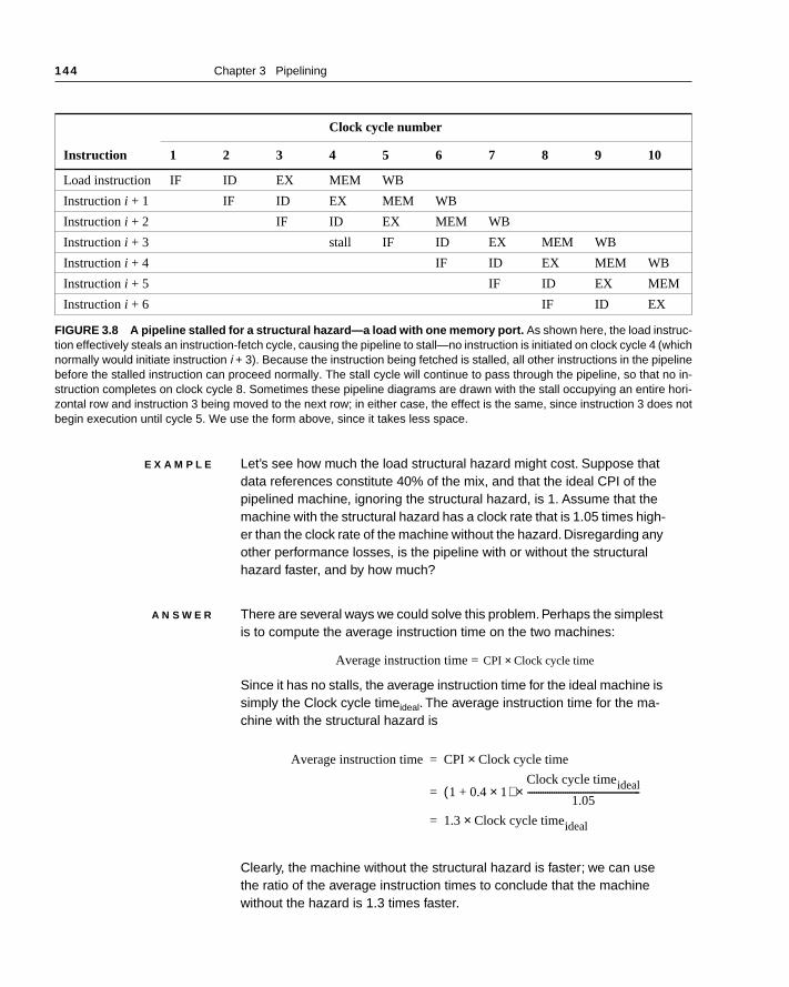
E X A M P L E Let’s see how much the load structural hazard might cost. Suppose that data references constitute 40% of the mix, and that the ideal CPI of the pipelined machine, ignoring the structural hazard, is 1. Assume that the machine with the structural hazard has a clock rate that is 1.05 times high-er than the clock rate of the machine without the hazard. Disregarding any other performance losses, is the pipeline with or without the structural hazard faster, and by how much?
A N S W E R There are several ways we could solve this problem. Perhaps the simplest is to compute the average instruction time on the two machines:
Average instruction time =
Since it has no stalls, the average instruction time for the ideal machine is simply the Clock cycle timeideal. The average instruction time for the ma-chine with the structural hazard is
Clearly, the machine without the structural hazard is faster; we can use the ratio of the average instruction times to conclude that the machine without the hazard is 1.3 times faster.
Clock cycle number
Instruction 1 2 3 4 5 6 7 8 9 10
Load instruction IF ID EX MEM WB
Instruction i + 1 IF ID EX MEM WB
Instruction i + 2 IF ID EX MEM WB
Instruction i + 3 stall IF ID EX MEM WB
Instruction i + 4 IF ID EX MEM WB
Instruction i + 5 IF ID EX MEM
Instruction i + 6 IF ID EX
FIGURE 3.8 A pipeline stalled for a structural hazard—a load with one memory port. As shown here, the load instruc-tion effectively steals an instruction-fetch cycle, causing the pipeline to stall—no instruction is initiated on clock cycle 4 (whichnormally would initiate instruction i + 3). Because the instruction being fetched is stalled, all other instructions in the pipelinebefore the stalled instruction can proceed normally. The stall cycle will continue to pass through the pipeline, so that no in-struction completes on clock cycle 8. Sometimes these pipeline diagrams are drawn with the stall occupying an entire hori-zontal row and instruction 3 being moved to the next row; in either case, the effect is the same, since instruction 3 does notbegin execution until cycle 5. We use the form above, since it takes less space.
CPI Clock cycle time×
Average instruction time CPI Clock cycle time×=
1 0.4 1×+( )Clock cycle timeideal
1.05---------------------------------------------------×=
1.3 Clock cycle timeideal×=

3.3 The Major Hurdle of Pipelining—Pipeline Hazards 145
ayshere
ing allma-cle (to totalfullyaz-ual-h ancyple,ten-
re-antage
As an alternative to this structural hazard, the designer could provide a separate memory access for instructions, either by splitting the cache into separate instruction and data caches, or by using a set of buffers, usually called instruction buffers, to hold instructions. Both the split cache and instruction buffer ideas are discussed in Chapter 5. ■
If all other factors are equal, a machine without structural hazards will alwhave a lower CPI. Why, then, would a designer allow structural hazards? Tare two reasons: to reduce cost and to reduce the latency of the unit. Pipelinthe functional units, or duplicating them, may be too costly. For example, chines that support both an instruction and a data cache access every cyprevent the structural hazard of the above example) require twice as muchmemory bandwidth and often have higher bandwidth at the pins. Likewise, pipelining a floating-point multiplier consumes lots of gates. If the structural hard would not occur often, it may not be worth the cost to avoid it. It is also usly possible to design an unpipelined unit, or one that isn’t fully pipelined, witsomewhat shorter total delay than a fully pipelined unit. The shorter latecomes from the lack of pipeline registers that introduce overhead. For examboth the CDC 7600 and the MIPS R2010 floating-point unit choose shorter lacy (fewer clocks per operation) versus full pipelining. As we will see shortly,ducing latency has other performance benefits and may overcome the disadvof the structural hazard.
E X A M P L E Many recent machines do not have fully pipelined floating-point units. For example, suppose we had an implementation of DLX with a floating-point multiply unit but no pipelining. Assume the multiplier could accept a new multiply operation every five clock cycles. (This rate is called the repeat or initiation interval.) Will this structural hazard have a large or small perfor-mance impact on mdljdp2 running on DLX? For simplicity, assume that the floating-point multiplies are uniformly distributed.
A N S W E R From Chapter 2 we find that floating-point multiply has a frequency of 14% in mdljdp2. Our proposed pipeline can handle up to a 20% frequency of floating-point multiplies—one every five clock cycles. This means that the performance benefit of fully pipelining the floating-point multiply on mdljdp2 is likely to be limited, as long as the floating-point multiplies are not clustered but are distributed uniformly. In the best case, multiplies are overlapped with other operations, and there is no performance penalty at all. In the worst case, the multiplies are all clustered with no intervening instructions, and 14% of the instructions take 5 cycles each. Assuming a base CPI of 1, this amounts to an increase of 0.7 in the CPI.

146 Chapter 3 Pipelining
by haz- oper-utingn of
utd a
thatior to
ty
omhus,the
s in
im-eadsque,
In practice, examining the performance of mdljdp2 on a machine with a five-cycle-deep FP multiply pipeline shows that this structural hazard increases execution time by less than 3%. One reason this loss is so low is that data hazards (the topic of the next section) cause the pipeline to stall, preventing multiply instructions that might cause structural hazards from being initiated. Of course, other benchmarks make heavier use of floating-point multiply or have fewer data hazards, and thus would show a larger impact. In the rest of this chapter we will examine the contributions of these different types of stalls in the DLX pipeline. ■
A major effect of pipelining is to change the relative timing of instructions overlapping their execution. This introduces data and control hazards. Dataards occur when the pipeline changes the order of read/write accesses toands so that the order differs from the order seen by sequentially execinstructions on an unpipelined machine. Consider the pipelined executiothese instructions:
ADD R1,R2,R3
SUB R4,R1,R5
AND R6,R1,R7
OR R8,R1,R9
XOR R10,R1,R11
All the instructions after the ADD use the result of the ADD instruction. As shown inFigure 3.9, the ADD instruction writes the value of R1 in the WB pipe stage, bthe SUB instruction reads the value during its ID stage. This problem is calledata hazard. Unless precautions are taken to prevent it, the SUB instruction willread the wrong value and try to use it. In fact, the value used by the SUB instruc-tion is not even deterministic: Though we might think it logical to assume SUB would always use the value of R1 that was assigned by an instruction prADD, this is not always the case. If an interrupt should occur between the ADD andSUB instructions, the WB stage of the ADD will complete, and the value of R1 athat point will be the result of the ADD. This unpredictable behavior is obviouslunacceptable.
The AND instruction is also affected by this hazard. As we can see frFigure 3.9, the write of R1 does not complete until the end of clock cycle 5. Tthe AND instruction that reads the registers during clock cycle 4 will receive wrong results.
The XOR instruction operates properly, because its register read occurclock cycle 6, after the register write. The OR instruction can also be made tooperate without incurring a hazard by a simple implementation technique,plied in our pipeline diagrams. The technique is to perform the register file rin the second half of the cycle and the writes in the first half. This techni
3.4 Data Hazards

3.4 Data Hazards 147
ister
azard
nique
which is hinted at in earlier figures by placing the dashed box around the regfile, allows the OR instruction in the example in Figure 3.9 to execute correctly.
The next subsection discusses a technique to eliminate the stalls for the hinvolving the SUB and AND instructions.
Minimizing Data Hazard Stalls By Forwarding
The problem posed in Figure 3.9 can be solved with a simple hardware techcalled forwarding (also called bypassing and sometimes short-circuiting). Thekey insight in forwarding is that the result is not really needed by the SUB until af-ter the ADD actually produces it. If the result can be moved from where the ADD
FIGURE 3.9 The use of the result of the ADD instruction in the next three instructions causes a hazard, since theregister is not written until after those instructions read it.
CC 1 CC 2 CC 3 CC 4 CC 5 CC 6
Time (in clock cycles)
R1, R2, R3
Reg
DM
DM
DM
ADD
SUB R4, R1, R5
AND R6, R1, R7
OR R8, R1, R9
XOR R10, R1, R11
Reg
Reg Reg
RegIM
IM
IM
IM
IM
Reg ALU
ALU
ALU
ALU
Reg
Pro
gra
m e
xecu
tio
n o
rde
r (i
n i
nst
ruct
ion
s)

148 Chapter 3 Pipelining
ward-
U
rit- con-alue
t be-
fromrtedplaceence
func- theame
f R1uts. re-nalpaths In andex-
produces it, the EX/MEM register, to where the SUB needs it, the ALU inputlatches, then the need for a stall can be avoided. Using this observation, foring works as follows:
1. The ALU result from the EX/MEM register is always fed back to the ALinput latches.
2. If the forwarding hardware detects that the previous ALU operation has wten the register corresponding to a source for the current ALU operation,trol logic selects the forwarded result as the ALU input rather than the vread from the register file.
Notice that with forwarding, if the SUB is stalled, the ADD will be completed andthe bypass will not be activated. This is also true for the case of an interruptween the two instructions.
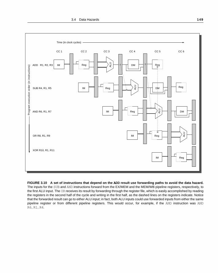
As the example in Figure 3.9 shows, we need to forward results not only the immediately previous instruction, but possibly from an instruction that statwo cycles earlier. Figure 3.10 shows our example with the bypass paths in and highlighting the timing of the register read and writes. This code sequcan be executed without stalls.
Forwarding can be generalized to include passing a result directly to the tional unit that requires it: A result is forwarded from the output of one unit toinput of another, rather than just from the result of a unit to the input of the sunit. Take, for example, the following sequence:
ADD R1,R2,R3
LW R4,0(R1)
SW 12(R1),R4
To prevent a stall in this sequence, we would need to forward the values oand R4 from the pipeline registers to the ALU and data memory inpFigure 3.11 shows all the forwarding paths for this example. In DLX, we mayquire a forwarding path from any pipeline register to the input of any functiounit. Because the ALU and data memory both accept operands, forwarding are needed to their inputs from both the ALU/MEM and MEM/WB registers.addition, DLX uses a zero detection unit that operates during the EX cycle,forwarding to that unit will be needed as well. Later in this section we will plore all the necessary forwarding paths and the control of those paths.
3.4 Data Hazards 149
FIGURE 3.10 A set of instructions that depend on the ADD result use forwarding paths to avoid the data hazard.The inputs for the SUB and AND instructions forward from the EX/MEM and the MEM/WB pipeline registers, respectively, tothe first ALU input. The OR receives its result by forwarding through the register file, which is easily accomplished by readingthe registers in the second half of the cycle and writing in the first half, as the dashed lines on the registers indicate. Noticethat the forwarded result can go to either ALU input; in fact, both ALU inputs could use forwarded inputs from either the samepipeline register or from different pipeline registers. This would occur, for example, if the AND instruction was ANDR6, R1, R4.
DM
DM
DM
CC 1 CC 2 CC 3 CC 4 CC 5 CC 6
Time (in clock cycles)
ADD R1, R2, R3
SUB R4, R1, R5
AND R6, R1, R7
OR R8, R1, R9
XOR R10, R1, R11
Reg
Reg
ALU
ALU
ALU
ALU
Reg
Reg
RegIM
IM
IM
IM
IM
Reg
Reg
Pro
gra
m e
xecu
tio
n o
rde
r (i
n i
nst
ruct
ion
s)

150 Chapter 3 Pipelining
s, andhe or-ter op-ce byver, fromr if werlierelinetion
Data Hazard Classification
A hazard is created whenever there is a dependence between instructionthey are close enough that the overlap caused by pipelining would change tder of access to an operand. Our example hazards have all been with regiserands, but it is also possible for a pair of instructions to create a dependenwriting and reading the same memory location. In our DLX pipeline, howememory references are always kept in order, preventing this type of hazardarising. Cache misses could cause the memory references to get out of ordeallowed the processor to continue working on later instructions, while an eainstruction that missed the cache was accessing memory. For the DLX pipwe stall the entire pipeline on a cache miss, effectively making the instruc
FIGURE 3.11 Stores require an operand during MEM, and forwarding of that operand is shownhere. The result of the load is forwarded from the memory output in MEM/WB to the memory input to bestored. In addition, the ALU output is forwarded to the ALU input for the address calculation of both the loadand the store (this is no different than forwarding to another ALU operation). If the store depended on animmediately preceding ALU operation (not shown above), the result would need to be forwarded to preventa stall.
CC 1 CC 2 CC 3 CC 4 CC 5 CC 6
Time (in clock cycles)
R1, R2, R3 DM
DM
DM
ADD
LW R4, 0(R1)
SW 12(R1), R4
Reg
Reg Reg
RegIM
IM
IM ALU
ALU
ALU
Reg
Pro
gra
m e
xecu
tio
n o
rde
r (i
n i
nst
ruct
ion
s)

3.4 Data Hazards 151
willfferentaz-
orders areeline.
kind
writ-
n in- in-s. Ifible.ge,emoryng thee re-
pipe-
twos theand
elinezardtruc-line.
that contained the miss run for multiple clock cycles. In the next chapter, wediscuss machines that allow loads and stores to be executed in an order difrom that in the program, which will introduce new problems. All the data hards discussed in this chapter involve registers within the CPU.
Data hazards may be classified as one of three types, depending on theof read and write accesses in the instructions. By convention, the hazardnamed by the ordering in the program that must be preserved by the pipConsider two instructions i and j, with i occurring before j. The possible data haz-ards are
■ RAW (read after write) — j tries to read a source before i writes it, so j incor-rectly gets the old value. This is the most common type of hazard and thethat we used forwarding to overcome in Figures 3.10 and 3.11.
■ WAW (write after write) — j tries to write an operand before it is written by i.The writes end up being performed in the wrong order, leaving the value ten by i rather than the value written by j in the destination. This hazard ispresent only in pipelines that write in more than one pipe stage (or allow astruction to proceed even when a previous instruction is stalled). The DLXteger pipeline writes a register only in WB and avoids this class of hazardwe made two changes to the DLX pipeline, WAW hazards would be possFirst, we could move write back for an ALU operation into the MEM stasince the data value is available by then. Second, suppose that the data maccess took two pipe stages. Here is a sequence of two instructions showiexecution in this revised pipeline, highlighting the pipe stage that writes thsult:
Unless this hazard is avoided, execution of this sequence on this revisedline will leave the result of the first write (the LW) in R1, rather than the resultof the ADD!
Allowing writes in different pipe stages introduces other problems, since instructions can try to write during the same clock cycle. When we discusDLX FP pipeline (section 3.7), which has both writes in different stages different pipeline lengths, we will deal with both write conflicts and WAWhazards in detail.
■ WAR (write after read) — j tries to write a destination before it is read by i,so i incorrectly gets the new value. This cannot happen in our example pipbecause all reads are early (in ID) and all writes are late (in WB). This haoccurs when there are some instructions that write results early in the instion pipeline, and other instructions that read a source late in the pipe
LW R1,0(R2) IF ID EX MEM1 MEM2 WB
ADD R1,R2,R3 IF ID EX WB

152 Chapter 3 Pipelining
s be-ctionad late ase valueing
rs:
, wecuted
sing.
n inop-le 4in-d in-3.12apa-
eed-
Because of the natural structure of a pipeline, which typically reads valuefore it writes results, such hazards are rare. Pipelines for complex instrusets that support autoincrement addressing and require operands to be rein the pipeline could create a WAR hazard. If we modified the DLX pipelinein the above example and also read some operands late, such as the sourcfor a store instruction, a WAR hazard could occur. Here is the pipeline timfor such a potential hazard, highlighting the stage where the conflict occu
If the SW reads R2 during the second half of its MEM2 stage and the ADD writesR2 during the first half of its WB stage, the SW will incorrectly read and storethe value produced by the ADD. In the DLX pipeline, reading all operands fromthe register file during ID avoids this hazard; however, in the next chapterwill see how these hazards occur more easily when instructions are exeout of order.
Note that the RAR (read after read) case is not a hazard.
Data Hazards Requiring Stalls
Unfortunately, not all potential data hazards can be handled by bypasConsider the following sequence of instructions:
LW R1,0(R2)
SUB R4,R1,R5
AND R6,R1,R7
OR R8,R1,R9
The pipelined datapath with the bypass paths for this example is showFigure 3.12. This case is different from the situation with back-to-back ALU erations. The LW instruction does not have the data until the end of clock cyc(its MEM cycle), while the SUB instruction needs to have the data by the begning of that clock cycle. Thus, the data hazard from using the result of a loastruction cannot be completely eliminated with simple hardware. As Figure shows, such a forwarding path would have to operate backward in time—a cbility not yet available to computer designers! We can forward the result immedi-ately to the ALU from the MEM/WB registers for use in the AND operation, whichbegins two clock cycles after the load. Likewise, the OR instruction has no prob-lem, since it receives the value through the register file. For the SUB instruction,the forwarded result arrives too late—at the end of a clock cycle, when it is ned at the beginning.
SW 0(R1),R2 IF ID EX MEM1 MEM2 WB
ADD R2,R3,R4 IF ID EX WB

3.4 Data Hazards 153
for-
rlockuntilll or the this in
s se-one
The load instruction has a delay or latency that cannot be eliminated bywarding alone. Instead, we need to add hardware, called a pipeline interlock, topreserve the correct execution pattern. In general, a pipeline interlock detects ahazard and stalls the pipeline until the hazard is cleared. In this case, the intestalls the pipeline, beginning with the instruction that wants to use the data the source instruction produces it. This pipeline interlock introduces a stabubble, just as it did for the structural hazard in section 3.3. The CPI forstalled instruction increases by the length of the stall (one clock cycle incase). The pipeline with the stall and the legal forwarding is shownFigure 3.13. Because the stall causes the instructions starting with the SUB tomove one cycle later in time, the forwarding to the AND instruction now goesthrough the register file, and no forwarding at all is needed for the OR instruction.The insertion of the bubble causes the number of cycles to complete thiquence to grow by one. No instruction is started during clock cycle 4 (and n
FIGURE 3.12 The load instruction can bypass its results to the AND and OR instructions, but not to the SUB, sincethat would mean forwarding the result in “negative time.”
DMALU
ALU
ALU
DM
CC 1 CC 2 CC 3 CC 4 CC 5
Time (in clock cycles)
LW R1, 0(R2)
SUB R4, R1, R5
AND R6, R1, R7
OR R8, R1, R9
Reg
Reg
RegIM
IM
IM
IM Reg
Reg
Pro
gra
m e
xecu
tio
n o
rde
r (i
n i
nst
ruct
ion
s)
154 Chapter 3 Pipelining
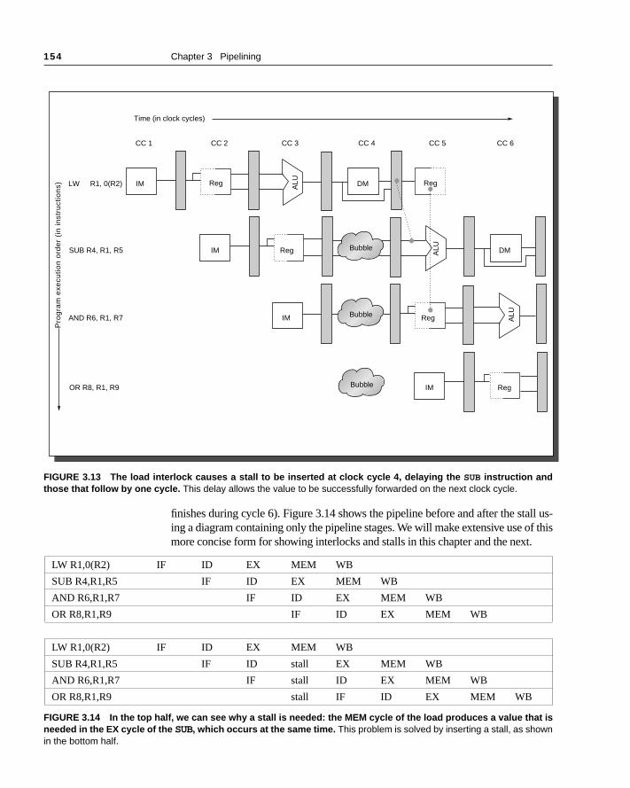
ll us-f this.
finishes during cycle 6). Figure 3.14 shows the pipeline before and after the staing a diagram containing only the pipeline stages. We will make extensive use omore concise form for showing interlocks and stalls in this chapter and the next
FIGURE 3.13 The load interlock causes a stall to be inserted at clock cycle 4, delaying the SUB instruction andthose that follow by one cycle. This delay allows the value to be successfully forwarded on the next clock cycle.
LW R1,0(R2) IF ID EX MEM WB
SUB R4,R1,R5 IF ID EX MEM WB
AND R6,R1,R7 IF ID EX MEM WB
OR R8,R1,R9 IF ID EX MEM WB
LW R1,0(R2) IF ID EX MEM WB
SUB R4,R1,R5 IF ID stall EX MEM WB
AND R6,R1,R7 IF stall ID EX MEM WB
OR R8,R1,R9 stall IF ID EX MEM WB
FIGURE 3.14 In the top half, we can see why a stall is needed: the MEM cycle of the load produces a value that isneeded in the EX cycle of the SUB, which occurs at the same time. This problem is solved by inserting a stall, as shownin the bottom half.
DM
DM
CC 1 CC 2 CC 3 CC 4 CC 5 CC 6
Time (in clock cycles)
LW R1, 0(R2)
SUB R4, R1, R5
AND R6, R1, R7
OR R8, R1, R9
Reg ALU
ALU
ALU
Reg
Reg
RegIM
IM
IM
IM Reg
Pro
gra
m e
xecu
tio
n o
rde
r (i
n i
nst
ruct
ion
s)
Bubble
Bubble
Bubble

3.4 Data Hazards 155
enal-and
for a valuece there.
duleinateith aech-
chines
E X A M P L E Suppose that 30% of the instructions are loads, and half the time the in-struction following a load instruction depends on the result of the load. If this hazard creates a single-cycle delay, how much faster is the ideal pipe-lined machine (with a CPI of 1) that does not delay the pipeline than the real pipeline? Ignore any stalls other than pipeline stalls.
A N S W E R The ideal machine will be faster by the ratio of the CPIs. The CPI for an instruction following a load is 1.5, since it stalls half the time. Because loads are 30% of the mix, the effective CPI is (0.7 × 1 + 0.3 × 1.5) = 1.15. This means that the ideal machine is 1.15 times faster. ■
In the next subsection we consider compiler techniques to reduce these pties. After that, we look at how to implement hazard detection, forwarding, interlocks.
Compiler Scheduling for Data Hazards
Many types of stalls are quite frequent. The typical code-generation patternstatement such as A = B + C produces a stall for a load of the second data(C). Figure 3.15 shows that the store of A need not cause another stall, sinresult of the addition can be forwarded to the data memory for use by the sto
Rather than just allow the pipeline to stall, the compiler could try to schethe pipeline to avoid these stalls by rearranging the code sequence to elimthe hazard. For example, the compiler could try to avoid generating code wload followed by the immediate use of the load destination register. This tnique, called pipeline scheduling or instruction scheduling, was first used in the1960s and became an area of major interest in the 1980s, as pipelined mabecame more widespread.
E X A M P L E Generate DLX code that avoids pipeline stalls for the following sequence:
a = b + c;
d = e – f;
Assume loads have a latency of one clock cycle.
LW R1,B IF ID EX MEM WB
LW R2,C IF ID EX MEM WB
ADD R3,R1,R2 IF ID stall EX MEM WB
SW A,R3 IF stall ID EX MEM WB
FIGURE 3.15 The DLX code sequence for A = B + C. The ADD instruction must be stalled to allow the load of C to com-plete. The SW need not be delayed further because the forwarding hardware passes the result from the MEM/WB directly tothe data memory input for storing.

156 Chapter 3 Pipelining
linesing
ulingock isnces. Fornlyis ad-sults,re ef-ismctive these
(ID)
eline.
A N S W E R Here is the scheduled code:
LW Rb,b
LW Rc,c
LW Re,e ; swap instructions to avoid stall
ADD Ra,Rb,Rc
LW Rf,f
SW a,Ra ; store/load exchanged to avoid stall
SUB Rd,Re,Rf
SW d,Rd
Both load interlocks (LW Rc, c to ADD Ra, Rb, Rc and LW Rf , f to SUB Rd, Re, Rf ) have been eliminated. There is a dependence between the ALU instruction and the store, but the pipeline structure allows the re-sult to be forwarded. Notice that the use of different registers for the first and second statements was critical for this schedule to be legal. In partic-ular, if the variable e was loaded into the same register as b or c, this schedule would be illegal. In general, pipeline scheduling can increase the register count required. In the next chapter, we will see that this in-crease can be substantial for machines that can issue multiple instruc-tions in one clock. ■
Many modern compilers try to use instruction scheduling to improve pipeperformance. In the simplest algorithms, the compiler simply schedules uother instructions in the same basic block. A basic block is a straight-line code se-quence with no transfers in or out, except at the beginning or end. Schedsuch code sequences is easy, since we know that every instruction in the blexecuted if the first one is. We can simply make a graph of the dependeamong the instructions and order the instructions so as to minimize the stallsa simple pipeline like the DLX integer pipeline with only short latencies (the odelay is one cycle on loads), a scheduling strategy focusing on basic blocks equate. Figure 3.16 shows the frequency that stalls are required for load reassuming a single-cycle delay for loads. As you can see, this process is mofective for floating-point programs that have significant amounts of parallelamong instructions. As pipelining becomes more extensive and the effepipeline latencies grow, more ambitious scheduling schemes are needed;are discussed in detail in the next chapter.
Implementing the Control for the DLX Pipeline
The process of letting an instruction move from the instruction decode stageinto the execution stage (EX) of this pipeline is usually called instruction issue;an instruction that has made this step is said to have issued. For the DLX integerpipeline, all the data hazards can be checked during the ID phase of the pip

3.4 Data Hazards 157
, weriatewareas up-tively, uses tworce
anmust
If a data hazard exists, the instruction is stalled before it is issued. Likewisecan determine what forwarding will be needed during ID and set the appropcontrols then. Detecting interlocks early in the pipeline reduces the hardcomplexity because the hardware never has to suspend an instruction that hdated the state of the machine, unless the entire machine is stalled. Alternawe can detect the hazard or forwarding at the beginning of a clock cycle thatan operand (EX and MEM for this pipeline). To show the differences in theseapproaches, we will show how the interlock for a RAW hazard with the soucoming from a load instruction (called a load interlock) can be implemented by acheck in ID, while the implementation of forwarding paths to the ALU inputs cbe done during EX. Figure 3.17 lists the variety of circumstances that we handle.
FIGURE 3.16 Percentage of the loads that result in a stall with the DLX pipeline. Thischart shows the frequency of stalls remaining in scheduled code that was globally optimizedbefore scheduling. Global optimization actually makes scheduling relatively harder becausethere are fewer candidates for scheduling into delay slots, as we discuss in Fallacies and Pit-falls. The pipeline slot after a load is often called the load delay or delay slot. In general, it iseasier to schedule the delay slots in FP programs, since they are more regular and the anal-ysis is easier. Hence fewer loads stall in the FP programs: an average of 13% of the loadsversus 25% on the integer programs. The actual performance impact depends on the loadfrequency, which varies from 19% to 34% with an average of 24%.The contribution to CPIruns from 0.01 cycles per instruction to 0.15 cycles per instruction.
Benchmark
com
pres
s
eqnt
ott
espr
esso gc
c li
dodu
cea
r
hydr
o2d
mdlj
dp
su2c
or
24%
41%
12%
23%24%
20% 20%
10% 10%
4%
0%
5%
10%
15%
20%
25%
30%
35%
40%
45%
Fraction of loads that cause a stall

158 Chapter 3 Pipelining
ithtagee canirect-l load
Let’s start with implementing the load interlock. If there is a RAW hazard wthe source instruction being a load, the load instruction will be in the EX swhen an instruction that needs the load data will be in the ID stage. Thus, wdescribe all the possible hazard situations with a small table, which can be dly translated to an implementation. Figure 3.18 shows a table that detects alinterlocks when the instruction using the load result is in the ID stage.
Situation Example code sequence Action
No dependence LW R1,45(R2)ADD R5,R6,R7SUB R8,R6,R7OR R9,R6,R7
No hazard possible because no dependence exists on R1 in the immediately following three instructions.
Dependencerequiring stall
LW R1,45(R2)ADD R5, R1,R7SUB R8,R6,R7OR R9,R6,R7
Comparators detect the use of R1 in the ADD and stall the ADD (and SUB and OR) before the ADD begins EX.
Dependence overcome by forwarding
LW R1,45(R2)ADD R5,R6,R7SUB R8, R1,R7OR R9,R6,R7
Comparators detect use of R1 in SUB and for-ward result of load to ALU in time for SUB to begin EX.
Dependence with accesses in order
LW R1,45(R2)ADD R5,R6,R7SUB R8,R6,R7OR R9, R1,R7
No action required because the read of R1 byOR occurs in the second half of the ID phase, while the write of the loaded data occurred in the first half.
FIGURE 3.17 Situations that the pipeline hazard detection hardware can see by com-paring the destination and sources of adjacent instructions. This table indicates that theonly comparison needed is between the destination and the sources on the two instructionsfollowing the instruction that wrote the destination. In the case of a stall, the pipeline depen-dences will look like the third case once execution continues. Of course hazards that involveR0 can be ignored since the register always contains 0, and the test above could be extendedto do this.
Opcode field of ID/EX (ID/EX.IR 0..5) Opcode field of IF/ID (IF/ID.IR 0..5) Matching operand fields
Load Register-register ALU ID/EX.IR11..15 == IF/ID.IR6..10
Load Register-register ALU ID/EX.IR11..15 == IF/ID.IR11..15
Load Load, store, ALU immediate, or branch ID/EX.IR11..15 == IF/ID.IR6..10
FIGURE 3.18 The logic to detect the need for load interlocks during the ID stage of an instruction requires threecomparisons. Lines 1 and 2 of the table test whether the load destination register is one of the source registers for aregister-register operation in ID. Line 3 of the table determines if the load destination register is a source for a load or storeeffective address, an ALU immediate, or a branch test. Remember that the IF/ID register holds the state of the instruction inID, which potentially uses the load result, while ID/EX holds the state of the instruction in EX, which is the potential loadinstruction.

3.4 Data Hazards 159
e stallaid inrry-us,/EX
doestsm-mpar-eous
s to thatource ortec-
tina-insters.re thetly
ed tot unit,estina-
eter-ge thegis-mentss in
sim- ex- to
Once a hazard has been detected, the control unit must insert the pipelinand prevent the instructions in the IF and ID stages from advancing. As we ssection 3.2, all the control information is carried in the pipeline registers. (Caing the instruction along is enough, since all control is derived from it.) Thwhen we detect a hazard we need only change the control portion of the IDpipeline register to all 0s, which happens to be a no-op (an instruction that nothing, such as ADD R0,R0,R0 ). In addition, we simply recirculate the contenof the IF/ID registers to hold the stalled instruction. In a pipeline with more coplex hazards, the same ideas would apply: We can detect the hazard by coing some set of pipeline registers and shift in no-ops to prevent erronexecution.
Implementing the forwarding logic is similar, though there are more caseconsider. The key observation needed to implement the forwarding logic isthe pipeline registers contain both the data to be forwarded as well as the sand destination register fields. All forwarding logically happens from the ALUdata memory output to the ALU input, the data memory input, or the zero detion unit. Thus, we can implement the forwarding by a comparison of the destion registers of the IR contained in the EX/MEM and MEM/WB stages agathe source registers of the IR contained in the ID/EX and EX/MEM registFigure 3.19 shows the comparisons and possible forwarding operations whedestination of the forwarded result is an ALU input for the instruction currenin EX. The Exercises ask you to add the entries when the result is forwardthe data memory. The last possible forwarding destination is the zero detecwhose forwarding paths look the same as those that are needed when the dtion instruction is an ALU immediate.
In addition to the comparators and combinational logic that we need to dmine when a forwarding path needs to be enabled, we also need to enlarmultiplexers at the ALU inputs and add the connections from the pipeline reters that are used to forward the results. Figure 3.20 shows the relevant segof the pipelined datapath with the additional multiplexers and connectionplace.
For DLX, the hazard detection and forwarding hardware is reasonably ple; we will see that things become somewhat more complicated when wetend this pipeline to deal with floating point. Before we do that, we needhandle branches.

160 Chapter 3 Pipelining
Pipeline register containing source instruction
Opcodeof sourceinstruction
Pipeline register containing destination instruction
Opcode of destination instruction
Destination of the forwarded result
Comparison(if equal then forward)
EX/MEM Register-register ALU
ID/EX Register-register ALU, ALU immediate, load, store, branch
Top ALU input
EX/MEM.IR16..20 == ID/EX.IR6..10
EX/MEM Register-register ALU
ID/EX Register-register ALU Bottom ALU input
EX/MEM.IR16..20 == ID/EX.IR11..15
MEM/WB Register-register ALU
ID/EX Register-register ALU, ALU immediate, load, store, branch
Top ALU input
MEM/WB.IR16..20 == ID/EX.IR6..10
MEM/WB Register-register ALU
ID/EX Register-register ALU Bottom ALU input
MEM/WB.IR16..20 == ID/EX.IR11..15
EX/MEM ALU immediate
ID/EX Register-register ALU, ALU immediate, load, store, branch
Top ALU input
EX/MEM.IR11..15 == ID/EX.IR6..10
EX/MEM ALU immediate
ID/EX Register-register ALU Bottom ALU input
EX/MEM.IR11..15 == ID/EX.IR11..15
MEM/WB ALU immediate
ID/EX Register-register ALU, ALU immediate, load, store, branch
Top ALU input
MEM/WB.IR11..15 == ID/EX.IR6..10
MEM/WB ALU immediate
ID/EX Register-register ALU Bottom ALU input
MEM/WB.IR11..15 == ID/EX.IR11..15
MEM/WB Load ID/EX Register-register ALU, ALU immediate, load, store, branch
Top ALU input
MEM/WB.IR11..15 == ID/EX.IR6..10
MEM/WB Load ID/EX Register-register ALU Bottom ALU input
MEM/WB.IR11..15 == ID/EX.IR11..15
FIGURE 3.19 Forwarding of data to the two ALU inputs (for the instruction in EX) can occur from the ALU result(in EX/MEM or in MEM/WB) or from the load result in MEM/WB. There are 10 separate comparisons needed to tell wheth-er a forwarding operation should occur. The top and bottom ALU inputs refer to the inputs corresponding to the first andsecond ALU source operands, respectively, and are shown explicitly in Figure 3.1 on page 130 and in Figure 3.20 onpage 161. Remember that the pipeline latch for destination instruction in EX is ID/EX, while the source values come fromthe ALUOutput portion of EX/MEM or MEM/WB or the LMD portion of MEM/WB. There is one complication not addressedby this logic: dealing with multiple instructions that write the same register. For example, during the code sequence ADD R1,R2, R3; ADDI R1, R1, #2; SUB R4, R3, R1, the logic must ensure that the SUB instruction uses the result of the ADDIinstruction rather than the result of the ADD instruction. The logic shown above can be extended to handle this case by simplytesting that forwarding from MEM/WB is enabled only when forwarding from EX/MEM is not enabled for the same input. Be-cause the ADDI result will be in EX/MEM, it will be forwarded, rather than the ADD result in MEM/WB.

3.5 Control Hazards 161
han PC tos the
edom-
soone newtruc- pipe-ust
Control hazards can cause a greater performance loss for our DLX pipeline tdo data hazards. When a branch is executed, it may or may not change thesomething other than its current value plus 4. Recall that if a branch changePC to its target address, it is a taken branch; if it falls through, it is not taken, oruntaken. If instruction i is a taken branch, then the PC is normally not changuntil the end of MEM, after the completion of the address calculation and cparison, as shown in Figure 3.4 (page 134) and Figure 3.5 (page 136).
The simplest method of dealing with branches is to stall the pipeline as as we detect the branch until we reach the MEM stage, which determines thPC. Of course, we do not want to stall the pipeline until we know that the instion is a branch; thus, the stall does not occur until after the ID stage, and theline behavior looks like that shown in Figure 3.21. This control hazard stall m
FIGURE 3.20 Forwarding of results to the ALU requires the addition of three extra in-puts on each ALU multiplexer and the addition of three paths to the new inputs. Thepaths correspond to a bypass of (1) the ALU output at the end of the EX, (2) the ALU outputat the end of the MEM stage, and (3) the memory output at the end of the MEM stage.
3.5 Control Hazards
Datamemory
ALU
Zero?
ID/EX EX/MEM MEM/WB
Mux
Mux

162 Chapter 3 Pipelining
e in-ranchormso for repe-deedly, but
30%ievesche re-
to ex- early
yle byn ond ear-ddersablearate stalls thatin-
be implemented differently from a data hazard stall, since the IF cycle of thstruction following the branch must be repeated as soon as we know the boutcome. Thus, the first IF cycle is essentially a stall, because it never perfuseful work. This stall can be implemented by setting the IF/ID register to zerthe three cycles. You may have noticed that if the branch is untaken, then thetition of the IF stage is unnecessary since the correct instruction was infetched. We will develop several schemes to take advantage of this fact shortfirst, let’s examine how we could reduce the worst-case branch penalty.
Three clock cycles wasted for every branch is a significant loss. With a branch frequency and an ideal CPI of 1, the machine with branch stalls achonly about half the ideal speedup from pipelining! Thus, reducing the branpenalty becomes critical. The number of clock cycles in a branch stall can bduced by two steps:
1. Find out whether the branch is taken or not taken earlier in the pipeline.
2. Compute the taken PC (i.e., the address of the branch target) earlier.
To optimize the branch behavior, both of these must be done—it doesn’t help know the target of the branch without knowing whether the next instruction toecute is the target or the instruction at PC + 4. Both steps should be taken asin the pipeline as possible.
In DLX, the branches (BEQZ and BNEZ) require testing a register for equalitto zero. Thus, it is possible to complete this decision by the end of the ID cycmoving the zero test into that cycle. To take advantage of an early decisiowhether the branch is taken, both PCs (taken and untaken) must be computely. Computing the branch target address during ID requires an additional abecause the main ALU, which has been used for this function so far, is not uuntil EX. Figure 3.22 shows the revised pipelined datapath. With the sepadder and a branch decision made during ID, there is only a one-clock-cycleon branches. Although this reduces the branch delay to one cycle, it meanan ALU instruction followed by a branch on the result of the instruction will
Branch instruction IF ID EX MEM WB
Branch successor IF stall stall IF ID EX MEM WB
Branch successor + 1 IF ID EX MEM WB
Branch successor + 2 IF ID EX MEM
Branch successor + 3 IF ID EX
Branch successor + 4 IF ID
Branch successor + 5 IF
FIGURE 3.21 A branch causes a three-cycle stall in the DLX pipeline: One cycle is a repeated IF cycle and twocycles are idle. The instruction after the branch is fetched, but the instruction is ignored, and the fetch is restarted once thebranch target is known. It is probably obvious that if the branch is not taken, the second IF for branch successor is redundant.This will be addressed shortly.

3.5 Control Hazards 163
pipe-
yclespute
ecode
ess itentore,even.
ycles.ds on ex-at will
cur a data hazard stall. Figure 3.23 shows the branch portion of the revisedline table from Figure 3.5 (page 136).
In some machines, branch hazards are even more expensive in clock cthan in our example, since the time to evaluate the branch condition and comthe destination can be even longer. For example, a machine with separate dand register fetch stages will probably have a branch delay—the length of thecontrol hazard—that is at least one clock cycle longer. The branch delay, unlis dealt with, turns into a branch penalty. Many older machines that implemmore complex instruction sets have branch delays of four clock cycles or mand large, deeply pipelined machines often have branch penalties of six or sIn general, the deeper the pipeline, the worse the branch penalty in clock cOf course, the relative performance effect of a longer branch penalty depenthe overall CPI of the machine. A high CPI machine can afford to have morepensive branches because the percentage of the machine’s performance thbe lost from branches is less.
FIGURE 3.22 The stall from branch hazards can be reduced by moving the zero test and branch target calculationinto the ID phase of the pipeline. Notice that we have made two important changes, each of which removes one cycle fromthe three cycle stall for branches. The first change is to move both the branch address target calculation and the branchcondition decision to the ID cycle. The second change is to write the PC of the instruction in the IF phase, using either thebranch target address computed during ID or the incremented PC computed during IF. In comparison, Figure 3.4 obtainedthe branch target address from the EX/MEM register and wrote the result during the MEM clock cycle. As mentioned in Fig-ure 3.4, the PC can be thought of as a pipeline register (e.g., as part of ID/IF), which is written with the address of the nextinstruction at the end of each IF cycle.
Data
ALU
Signextend
16 32
memory
PC
Instructionmemory
ADD
ADD
IF/ID
4
EX/MEM MEM/WB
IR6..10
MEM/WB.IR
IR11..15
Registers
Zero?
Mux
Mux
Mux
IR
ID/EX
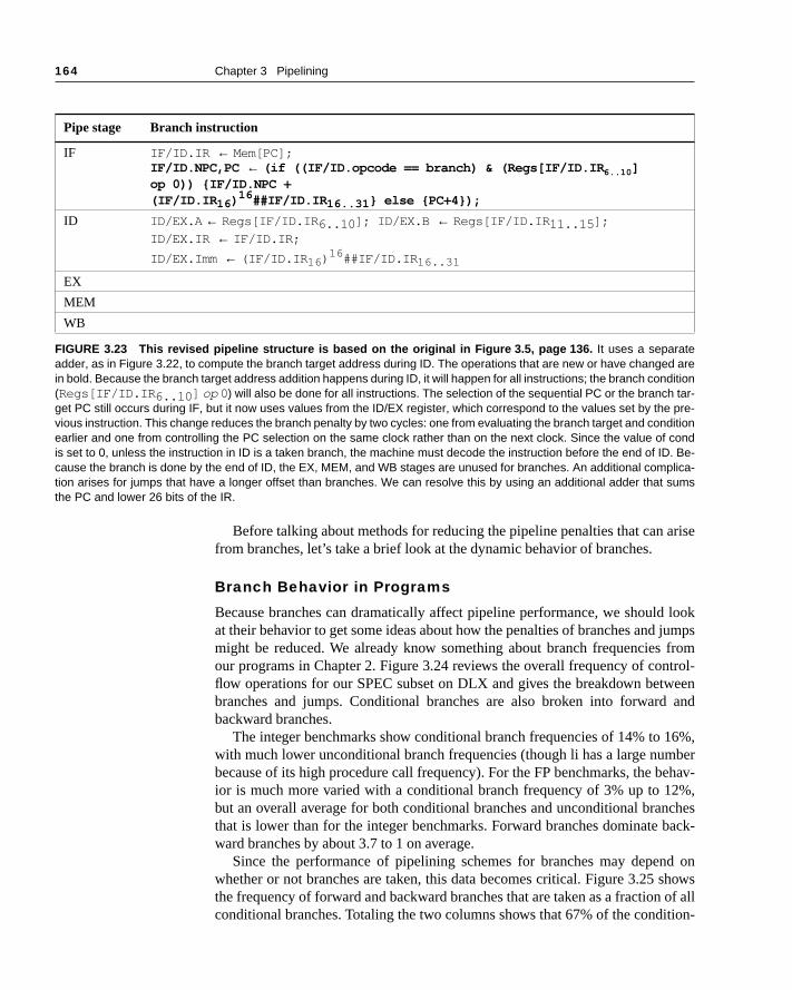
164 Chapter 3 Pipelining
arise
look jumpsfromtrol-een
and
6%,ber
ehav-2%,ches
back-
d onshows of alltion-
Before talking about methods for reducing the pipeline penalties that can from branches, let’s take a brief look at the dynamic behavior of branches.
Branch Behavior in Programs
Because branches can dramatically affect pipeline performance, we shouldat their behavior to get some ideas about how the penalties of branches andmight be reduced. We already know something about branch frequencies our programs in Chapter 2. Figure 3.24 reviews the overall frequency of conflow operations for our SPEC subset on DLX and gives the breakdown betwbranches and jumps. Conditional branches are also broken into forwardbackward branches.
The integer benchmarks show conditional branch frequencies of 14% to 1with much lower unconditional branch frequencies (though li has a large numbecause of its high procedure call frequency). For the FP benchmarks, the bior is much more varied with a conditional branch frequency of 3% up to 1but an overall average for both conditional branches and unconditional branthat is lower than for the integer benchmarks. Forward branches dominate ward branches by about 3.7 to 1 on average.
Since the performance of pipelining schemes for branches may depenwhether or not branches are taken, this data becomes critical. Figure 3.25 the frequency of forward and backward branches that are taken as a fractionconditional branches. Totaling the two columns shows that 67% of the condi
Pipe stage Branch instruction
IF IF/ID.IR ← Mem[PC]; IF/ID.NPC,PC ← (if ((IF/ID.opcode == branch) & (Regs[IF/ID.IR 6..10 ] op 0)) {IF/ID.NPC + (IF/ID.IR 16) 16##IF/ID.IR 16..31 } else {PC+4});
ID ID/EX.A ← Regs[IF/ID.IR 6..10 ]; ID/EX.B ← Regs[IF/ID.IR 11..15 ];
ID/EX.IR ← IF/ID.IR;
ID/EX.Imm ← (IF/ID.IR 16) 16##IF/ID.IR 16..31
EX
MEM
WB
FIGURE 3.23 This revised pipeline structure is based on the original in Figure 3.5, page 136. It uses a separateadder, as in Figure 3.22, to compute the branch target address during ID. The operations that are new or have changed arein bold. Because the branch target address addition happens during ID, it will happen for all instructions; the branch condition(Regs[IF/ID.IR 6..10 ] op 0) will also be done for all instructions. The selection of the sequential PC or the branch tar-get PC still occurs during IF, but it now uses values from the ID/EX register, which correspond to the values set by the pre-vious instruction. This change reduces the branch penalty by two cycles: one from evaluating the branch target and conditionearlier and one from controlling the PC selection on the same clock rather than on the next clock. Since the value of condis set to 0, unless the instruction in ID is a taken branch, the machine must decode the instruction before the end of ID. Be-cause the branch is done by the end of ID, the EX, MEM, and WB stages are unused for branches. An additional complica-tion arises for jumps that have a longer offset than branches. We can resolve this by using an additional adder that sumsthe PC and lower 26 bits of the IR.

3.5 Control Hazards 165
4 andich ishes
al branches are taken on average. By combining the data in Figures 3.23.25, we can compute the fraction of forward branches that are taken, whthe probability that a forward branch will be taken. Since backward branc
FIGURE 3.24 The frequency of instructions (branches, jumps, calls, and returns) thatmay change the PC. The unconditional column includes unconditional branches and jumps(these differ in how the target address is specified), procedure calls, and returns. In all thecases except li, the number of unconditional PC changes is roughly equally divided betweenthose that are for calls or returns and those that are unconditional jumps. In li, calls and re-turns outnumber jumps and unconditional branches by a factor of 3 (6% versus 2%). Sincethe compiler uses loop unrolling (described in detail in Chapter 4) as an optimization, thebackward conditional branch frequency will be lower, especially for the floating-point pro-grams. Overall, the integer programs average 13% forward conditional branches, 3% back-ward conditional branches, and 4% unconditional branches. The FP programs average 7%,2%, and 1%, respectively.
Percentage of instructions executed
0% 25%5% 10% 15% 20%
10%
0%
0%
2%
1%
2%
6%
4%4%
6%
2%2%
11%
8%4%
12%
4%3%
11%
1%4%
22%
2%2%
11%
3%3%
9%0%
1%
Forward conditionalbranches
Unconditional branchesBackward conditionalbranches
Benchmark
compress
eqntott
espresso
gcc
li
doduc
ear
hydro2d
mdljdp
su2cor

166 Chapter 3 Pipelining
be-eed,en on
h de-heseranchnalty
often form loops, we would expect that the probability of a backward branching taken is higher than the probability of a forward branch being taken. Indthe data, when combined, show that 60% of the forward branches are takaverage and 85% of the backward branches are taken.
Reducing Pipeline Branch Penalties
There are many methods for dealing with the pipeline stalls caused by branclay; we discuss four simple compile-time schemes in this subsection. In tfour schemes the actions for a branch are static—they are fixed for each bduring the entire execution. The software can try to minimize the branch pe
FIGURE 3.25 Together the forward and backward taken branches account for an average of 67% of all conditionalbranches. Although the backward branches are outnumbered, they are taken with a frequency that is almost 1.5 times high-er, contributing substantially to the taken branch frequency. On average, 62% of the branches are taken in the integer pro-grams and 70% in the FP programs. Note the wide disparity in behavior between a program like su2cor and mdljdp2; thesevariations make it challenging to predict the branch behavior very accurately. As in Figure 3.24, the use of loop unrollingaffects this data since it removes backward branches that had a high probability of being taken.
Fraction of allconditional branches
0%
80%
10%
20%
30%
40%
50%
70%
60%61%
21%
14%
53%
37%38%
26%
34%
13%
44%
16%
35%
25%
63%
8%
51%
22%
78%
3%
21%
Backward takenForward taken
Benchmarkco
mpr
ess
eqnt
ott
espr
esso gc
c li
dodu
cea
r
hydr
o2d
mdlj
dp2
su2c
or
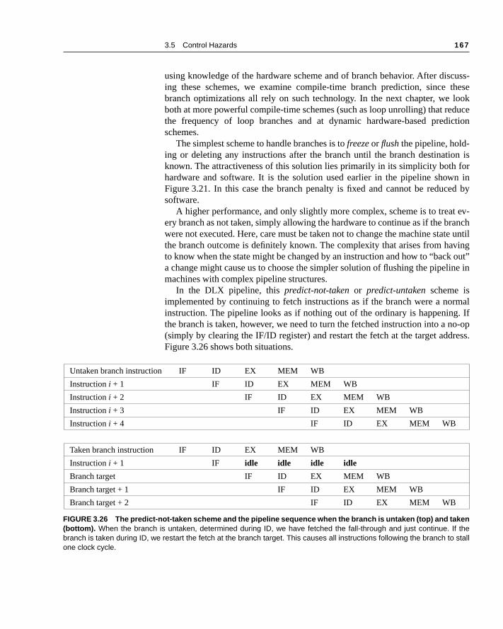
3.5 Control Hazards 167
cuss-theselookduceiction
n isforn in
ed by
t ev-anchte untilving out”ine in
rmal. Ifo-op
ress.
using knowledge of the hardware scheme and of branch behavior. After dising these schemes, we examine compile-time branch prediction, since branch optimizations all rely on such technology. In the next chapter, we both at more powerful compile-time schemes (such as loop unrolling) that rethe frequency of loop branches and at dynamic hardware-based predschemes.
The simplest scheme to handle branches is to freeze or flush the pipeline, hold-ing or deleting any instructions after the branch until the branch destinatioknown. The attractiveness of this solution lies primarily in its simplicity both hardware and software. It is the solution used earlier in the pipeline showFigure 3.21. In this case the branch penalty is fixed and cannot be reducsoftware.
A higher performance, and only slightly more complex, scheme is to treaery branch as not taken, simply allowing the hardware to continue as if the brwere not executed. Here, care must be taken not to change the machine stathe branch outcome is definitely known. The complexity that arises from hato know when the state might be changed by an instruction and how to “backa change might cause us to choose the simpler solution of flushing the pipelmachines with complex pipeline structures.
In the DLX pipeline, this predict-not-taken or predict-untaken scheme isimplemented by continuing to fetch instructions as if the branch were a noinstruction. The pipeline looks as if nothing out of the ordinary is happeningthe branch is taken, however, we need to turn the fetched instruction into a n(simply by clearing the IF/ID register) and restart the fetch at the target addFigure 3.26 shows both situations.
Untaken branch instruction IF ID EX MEM WB
Instruction i + 1 IF ID EX MEM WB
Instruction i + 2 IF ID EX MEM WB
Instruction i + 3 IF ID EX MEM WB
Instruction i + 4 IF ID EX MEM WB
Taken branch instruction IF ID EX MEM WB
Instruction i + 1 IF idle idle idle idle
Branch target IF ID EX MEM WB
Branch target + 1 IF ID EX MEM WB
Branch target + 2 IF ID EX MEM WB
FIGURE 3.26 The predict-not-taken scheme and the pipeline sequence when the branch is untaken (top) and taken(bottom). When the branch is untaken, determined during ID, we have fetched the fall-through and just continue. If thebranch is taken during ID, we restart the fetch at the branch target. This causes all instructions following the branch to stallone clock cycle.

168 Chapter 3 Pipelining
ranche takene we therehosenchedict-taken that pro-
nch,
DLX. In
An alternative scheme is to treat every branch as taken. As soon as the bis decoded and the target address is computed, we assume the branch to band begin fetching and executing at the target. Because in our DLX pipelindon’t know the target address any earlier than we know the branch outcome,is no advantage in this approach for DLX. In some machines—especially twith implicitly set condition codes or more powerful (and hence slower) braconditions—the branch target is known before the branch outcome, and a prtaken scheme might make sense. In either a predict-taken or predict-not-scheme, the compiler can improve performance by organizing the code sothe most frequent path matches the hardware’s choice. Our fourth schemevides more opportunities for the compiler to improve performance.
A fourth scheme in use in some machines is called delayed branch. This tech-nique is also used in many microprogrammed control units. In a delayed brathe execution cycle with a branch delay of length n is
branch instruction
sequential successor 1sequential successor 2
........sequential successor nbranch target if taken
The sequential successors are in the branch-delay slots. These instructions areexecuted whether or not the branch is taken. The pipeline behavior of the pipeline, which would have one branch-delay slot, is shown in Figure 3.27
Untaken branch instruction IF ID EX MEM WB
Branch-delay instruction (i + 1) IF ID EX MEM WB
Instruction i + 2 IF ID EX MEM WB
Instruction i + 3 IF ID EX MEM WB
Instruction i + 4 IF ID EX MEM WB
Taken branch instruction IF ID EX MEM WB
Branch-delay instruction (i + 1) IF ID EX MEM WB
Branch target IF ID EX MEM WB
Branch target + 1 IF ID EX MEM WB
Branch target + 2 IF ID EX MEM WB
FIGURE 3.27 The behavior of a delayed branch is the same whether or not the branch is taken. The instructions inthe delay slot (there is only one delay slot for DLX) are executed. If the branch is untaken, execution continues with the in-struction after the branch-delay instruction; if the branch is taken, execution continues at the branch target. When the in-struction in the branch-delay slot is also a branch, the meaning is unclear: if the branch is not taken, what should happen tothe branch in the branch-delay slot? Because of this confusion, architectures with delay branches often disallow putting abranch in the delay slot.

3.5 Control Hazards 169
, and
eful.hichts for
y win.
practice, all machines with delayed branch have a single instruction delaywe focus on that case.
The job of the compiler is to make the successor instructions valid and usA number of optimizations are used. Figure 3.28 shows the three ways in wthe branch delay can be scheduled. Figure 3.29 shows the different constraineach of these branch-scheduling schemes, as well as situations in which the
FIGURE 3.28 Scheduling the branch-delay slot. The top box in each pair shows thecode before scheduling; the bottom box shows the scheduled code. In (a) the delay slot isscheduled with an independent instruction from before the branch. This is the best choice.Strategies (b) and (c) are used when (a) is not possible. In the code sequences for (b) and(c), the use of R1 in the branch condition prevents the ADD instruction (whose destination isR1) from being moved after the branch. In (b) the branch-delay slot is scheduled from the tar-get of the branch; usually the target instruction will need to be copied because it can bereached by another path. Strategy (b) is preferred when the branch is taken with high proba-bility, such as a loop branch. Finally, the branch may be scheduled from the not-taken fallthrough as in (c). To make this optimization legal for (b) or (c), it must be OK to execute themoved instruction when the branch goes in the unexpected direction. By OK we mean thatthe work is wasted, but the program will still execute correctly. This is the case, for examplein case (b), if R4 were an unused temporary register when the branch goes in the unexpecteddirection.
(a) From before (b) From target (c) From fall through
SUB R4, R5, R6
ADD R1, R2, R3
if R1 = 0 then
ADD R1, R2, R3
if R1 = 0 then
SUB R4, R5, R6
SUB R4, R5, R6
ADD R1, R2, R3
if R1 = 0 then
OR R7, R8, R9ADD R1, R2, R3
if R1 = 0 then
SUB R4, R5, R6
ADD R1, R2, R3
if R2 = 0 then
if R2 = 0 then
ADD R1, R2, R3
BecomesBecomesBecomes
Delay slot
Delay slot
Delay slot
OR R7, R8, R9
SUB R4, R5, R6

170 Chapter 3 Pipelining
ionsity to, we im-ith
dict-y slot
theplyncel-
The limitations on delayed-branch scheduling arise from (1) the restricton the instructions that are scheduled into the delay slots and (2) our abilpredict at compile time whether a branch is likely to be taken or not. Shortlywill see how we can better predict branches statically at compile time. Toprove the ability of the compiler to fill branch delay slots, most machines wconditional branches have introduced a cancelling or nullifying branch. In a can-celling branch, the instruction includes the direction that the branch was preed. When the branch behaves as predicted, the instruction in the branch-delais simply executed as it would normally be with a delayed branch. Whenbranch is incorrectly predicted, the instruction in the branch-delay slot is simturned into a no-op. Figure 3.30 shows the behavior of a predicted-taken caling branch, both when the branch is taken and untaken.
Scheduling strategy Requirements Improves performance when?
(a) From before Branch must not depend on the rescheduled instruc-tions.
Always.
(b) From target Must be OK to execute rescheduled instructions if branch is not taken. May need to duplicate instruc-tions.
When branch is taken. May enlarge program if instructions are duplicated.
(c) From fall through Must be OK to execute instructions if branch is taken. When branch is not taken.
FIGURE 3.29 Delayed-branch scheduling schemes and their requirements. The origin of the instruction being sched-uled into the delay slot determines the scheduling strategy. The compiler must enforce the requirements when looking forinstructions to schedule the delay slot. When the slots cannot be scheduled, they are filled with no-op instructions. In strategy(b), if the branch target is also accessible from another point in the program—as it would be if it were the head of a loop—the target instructions must be copied and not just moved.
Untaken branch instruction IF ID EX MEM WB
Branch-delay instruction (i + 1) IF idle idle idle idle
Instruction i + 2 IF ID EX MEM WB
Instruction i + 3 IF ID EX MEM WB
Instruction i + 4 IF ID EX MEM WB
Taken branch instruction IF ID EX MEM WB
Branch-delay instruction (i + 1) IF ID EX MEM WB
Branch target IF ID EX MEM WB
Branch target + 1 IF ID EX MEM WB
Branch target + 2 IF ID EX MEM WB
FIGURE 3.30 The behavior of a predicted-taken cancelling branch depends on whether the branch is taken or not.The instruction in the delay slot is executed only if the branch is taken and is otherwise made into a no-op.

3.5 Control Hazards 171
entsedul-hown pro-llingges,nts of
th atakend then
hese can-ment)branch-t the
The advantage of cancelling branches is that they eliminate the requiremon the instruction placed in the delay slot, enabling the compiler to use sching schemes (b) and (c) of Figure 3.28 without meeting the requirements sfor these schemes in Figure 3.29. Most machines with cancelling branchesvide both a noncancelling form (i.e., a regular delayed branch) and a canceform, usually cancel if not taken. This combination gains most of the advantabut does not allow scheduling scheme (c) to be used unless the requiremeFigure 3.29 are met.
Figure 3.31 shows the effectiveness of the branch scheduling in DLX wisingle branch-delay slot and both a noncancelling branch and a cancel-if-unform. The compiler uses a standard delayed branch whenever possible anopts for a cancel-if-not-taken branch (also called branch likely). The second col-umn shows that almost 20% of the branch delay slots are filled with no-ops. Toccur when it is not possible to fill the delay slot, either because the potentialdidates are unknown (e.g., for a jump register that will be used in a case stateor because the successors are also branches. (Branches are not allowed in delay slots because of the confusion in semantics.) The table shows tha
Benchmark% conditional
branches
%conditional branches
with empty slots
%conditional branchesthat are
cancelling
%cancelling branchesthat are
cancelled
%branches
with cancelled delay slots
Total % branches with
empty or cancelleddelay slot
compress 14% 18% 31% 43% 13% 31%
eqntott 24% 24% 50% 24% 12% 36%
espresso 15% 29% 19% 21% 4% 33%
gcc 15% 16% 33% 34% 11% 27%
li 15% 20% 55% 48% 26% 46%
Integer average 17% 21% 38% 34% 13% 35%
doduc 8% 33% 12% 62% 7% 40%
ear 10% 37% 36% 14% 5% 42%
hydro2d 12% 0% 69% 24% 17% 17%
mdljdp2 9% 0% 86% 10% 9% 9%
su2cor 3% 7% 17% 57% 10% 17%
FP average 8% 16% 44% 33% 10% 25%
Overall average 12% 18% 41% 34% 12% 30%
FIGURE 3.31 Delayed and cancelling delay branches for DLX allow branch hazards to be hidden 70% of the timeon average for these 10 SPEC benchmarks. Empty delay slots cannot be filled at all (most often because the branch targetis another branch) in 18% of the branches. Just under half the conditional branches use a cancelling branch, and most ofthese are not cancelled (65%). The behavior varies widely across benchmarks. When the fraction of conditional branchesis added in, the contribution to CPI varies even more widely.

172 Chapter 3 Pipelining
d de-s aremar-llingstall
is ispilerxpos-ISCas at-oreh ap-thesemore the RISCclude
remaining 80% of the branch delay slots are filled nearly equally by standarlayed branches and by cancelling branches. Most of the cancelling branchenot cancelled and hence contribute to useful computation. Figure 3.32 sumizes the performance of the combination of delayed branch and cancebranch. Overall, 70% of the branch delays are usefully filled, reducing the penalty to 0.3 cycles per conditional branch.
Delayed branches are an architecturally visible feature of the pipeline. Ththe source both of their primary advantage—allowing the use of simple comscheduling to reduce branch penalties—and their primary disadvantage—eing an aspect of the implementation that is likely to change. In the early Rmachines with single-cycle branch delays, the delayed branch approach wtractive, since it yielded good performance with minimal hardware costs. Mrecently, with deeper pipelines and longer branch delays, a delayed brancproach is less useful since it cannot easily hide the longer delays. With longer branch delays, most architects have found it necessary to include powerful hardware schemes for branch prediction (which we will explore innext chapter), making the delayed branch superfluous.This has led to recentarchitectures that include both delayed and nondelayed branches or that inonly nondelayed branches, relying on hardware prediction.
FIGURE 3.32 The performance of delayed and cancelling branches is summarized byshowing the fraction of branches either with empty delay slots or with a cancelled de-lay slot. On average 30% of the branch delay slots are wasted. The integer programs are,on average, worse, wasting an average of 35% of the slots versus 25% for the FP programs.Notice, though, that two of the FP programs waste more branch delay slots than four of thefive integer programs.
Percentage ofconditional branches
0%
50%
5%
10%
15%
20%
25%
45%
30%
35%
40%
Canceled delay slotsEmpty slot
Benchmark
com
pres
s
eqnt
ott
espr
esso gc
c li
dodu
cea
r
hydr
o2d
mdlj
dp
su2c
or
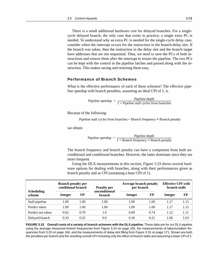
3.5 Control Hazards 173
ngle-PC is case,
ot. Iftargetoth in- PCse in-
pipe-
th un-y are
hard-n as
There is a small additional hardware cost for delayed branches. For a sicycle delayed branch, the only case that exists in practice, a single extra needed. To understand why an extra PC is needed for the single-cycle delayconsider when the interrupt occurs for the instruction in the branch-delay slthe branch was taken, then the instruction in the delay slot and the branch have addresses that are not sequential. Thus, we need to save the PCs of bstructions and restore them after the interrupt to restart the pipeline. The twocan be kept with the control in the pipeline latches and passed along with thstruction. This makes saving and restoring them easy.
Performance of Branch Schemes
What is the effective performance of each of these schemes? The effectiveline speedup with branch penalties, assuming an ideal CPI of 1, is
Because of the following:
Pipeline stall cycles from branches = Branch frequency × Branch penalty
we obtain
The branch frequency and branch penalty can have a component from boconditional and conditional branches. However, the latter dominate since themore frequent.
Using the DLX measurements in this section, Figure 3.33 shows several ware options for dealing with branches, along with their performances givebranch penalty and as CPI (assuming a base CPI of 1).
Schedulingscheme
Branch penalty perconditional branch Penalty per
unconditional branch
Average branch penaltyper branch
Effective CPI withbranch stalls
Integer FP Integer FP Integer FP
Stall pipeline 1.00 1.00 1.00 1.00 1.00 1.17 1.15
Predict taken 1.00 1.00 1.00 1.00 1.00 1.17 1.15
Predict not taken 0.62 0.70 1.0 0.69 0.74 1.12 1.11
Delayed branch 0.35 0.25 0.0 0.30 0.21 1.06 1.03
FIGURE 3.33 Overall costs of a variety of branch schemes with the DLX pipeline. These data are for our DLX pipelineusing the average measured branch frequencies from Figure 3.24 on page 165, the measurements of taken/untaken fre-quencies from 3.25 on page 166, and the measurements of delay-slot filling from Figure 3.31 on page 171. Shown are boththe penalties per branch and the resulting overall CPI including only the effect of branch stalls and assuming a base CPI of 1.
Pipeline speedupPipeline depth
1 Pipeline stall cycles from branches+---------------------------------------------------------------------------------------------=
Pipeline speedupPipeline depth
1 Branch frequency Branch penalty×+-----------------------------------------------------------------------------------------------=

174 Chapter 3 Pipelining
e anly oneas a.
Remember that the numbers in this section are dramatically affected by thelength of the pipeline delay and the base CPI. A longer pipeline delay will causincrease in the penalty and a larger percentage of wasted time. A delay of onclock cycle is small—the R4000 pipeline, which we examine in section 3.9, hconditional branch delay of three cycles. This results in a much higher penalty
E X A M P L E For an R4000-style pipeline, it takes three pipeline stages before the branch target address is known and an additional cycle before the branch condition is evaluated, assuming no stalls on the registers in the condi-tional comparison. This leads to the branch penalties for the three sim-plest prediction schemes listed in Figure 3.34.
Find the effective addition to the CPI arising from branches for this pipeline, using the data from the 10 SPEC benchmarks in Figures 3.24 and 3.25.
A N S W E R We find the CPIs by multiplying the relative frequency of unconditional, conditional untaken, and conditional taken branches by the respective penalties. These frequencies for the 10 SPEC programs are 4%, 6%, and 10%, respectively. The results are shown in Figure 3.35.
The differences among the schemes are substantially increased with this longer delay. If the base CPI was 1 and branches were the only source of stalls, the ideal pipeline would be 1.56 times faster than a
Branch scheme Penalty unconditional Penalty untaken Penalty taken
Flush pipeline 2 3 3
Predict taken 2 3 2
Predict untaken 2 0 3
FIGURE 3.34 Branch penalties for the three simplest prediction schemes for adeeper pipeline.
Addition to the CPI
Branch schemeUnconditional
branchesUntaken conditional
branchesTaken conditional
branches All branches
Frequency of event 4% 6% 10% 20%
Stall pipeline 0.08 0.18 0.30 0.56
Predict taken 0.08 0.18 0.20 0.46
Predict untaken 0.08 0.00 0.30 0.38
FIGURE 3.35 CPI penalties for three branch-prediction schemes and a deeper pipeline.

3.5 Control Hazards 175
e com-ctive-way aalso
ltak-n we
h, then
g how
henamicy oftatic
y ex-ctedmost
plestdiction
pipeline that used the stall-pipeline scheme. The predict-untaken scheme would be 1.13 times better than the stall-pipeline scheme under the same assumptions.
As we will see in section 3.9, the R4000 uses a mixed strategy with a one-cycle, cancelling delayed branch for the first cycle of the branch penalty. For an unconditional branch, a single-cycle stall is always added. For conditional branches, the remaining two cycles of the branch penalty use a predict-not-taken scheme. We will see measurements of the effec-tive branch penalties for this strategy later. ■
Static Branch Prediction: Using Compiler Technology
Delayed branches are a technique that exposes a pipeline hazard so that thpiler can reduce the penalty associated with the hazard. As we saw, the effeness of this technique partly depends on whether we correctly guess which branch will go. Being able to accurately predict a branch at compile time is helpful for scheduling data hazards. Consider the following code segment:
LW R1,0(R2)
SUB R1,R1,R3
BEQZ R1,L
OR R4,R5,R6
ADD R10,R4,R3
L: ADD R7,R8,R9
The dependence of the SUB and BEQZ on the LW instruction means that a stall wilbe needed after the LW. Suppose we knew that this branch was almost always en and that the value of R7 was not needed on the fall-through path. Thecould increase the speed of the program by moving the instruction ADD
R7,R8,R9 to the position after the LW. Correspondingly, if we knew the brancwas rarely taken and that the value of R4 was not needed on the taken pathwe could contemplate moving the OR instruction after the LW. In addition, we canalso use the information to better schedule any branch delay, since choosinto schedule the delay depends on knowing the branch behavior.
To perform these optimizations, we need to predict the branch statically wwe compile the program. In the next chapter, we will examine the use of dynprediction based on runtime program behavior. We will also look at a varietcompile-time methods for scheduling code; these techniques require sbranch prediction and thus the ideas in this section are critical.
There are two basic methods we can use to statically predict branches: bamination of the program behavior and by the use of profile information collefrom earlier runs of the program. We saw in Figure 3.25 (page 166) that branches were taken for both forward and backward branches. Thus, the simscheme is to predict a branch as taken. This scheme has an average mispre
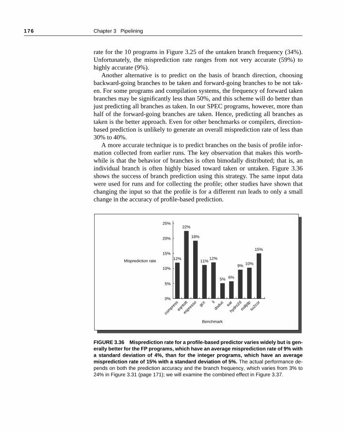
176 Chapter 3 Pipelining
4%).) to
singt tak-takenr than than
es astion-
than
nfor-orth-, an.36t data thatmall
rate for the 10 programs in Figure 3.25 of the untaken branch frequency (3Unfortunately, the misprediction rate ranges from not very accurate (59%highly accurate (9%).
Another alternative is to predict on the basis of branch direction, choobackward-going branches to be taken and forward-going branches to be noen. For some programs and compilation systems, the frequency of forward branches may be significantly less than 50%, and this scheme will do bettejust predicting all branches as taken. In our SPEC programs, however, morehalf of the forward-going branches are taken. Hence, predicting all branchtaken is the better approach. Even for other benchmarks or compilers, direcbased prediction is unlikely to generate an overall misprediction rate of less30% to 40%.
A more accurate technique is to predict branches on the basis of profile imation collected from earlier runs. The key observation that makes this wwhile is that the behavior of branches is often bimodally distributed; that isindividual branch is often highly biased toward taken or untaken. Figure 3shows the success of branch prediction using this strategy. The same inpuwere used for runs and for collecting the profile; other studies have shownchanging the input so that the profile is for a different run leads to only a schange in the accuracy of profile-based prediction.
FIGURE 3.36 Misprediction rate for a profile-based predictor varies widely but is gen-erally better for the FP programs, which have an average misprediction rate of 9% witha standard deviation of 4%, than for the integer programs, which have an averagemisprediction rate of 15% with a standard deviation of 5%. The actual performance de-pends on both the prediction accuracy and the branch frequency, which varies from 3% to24% in Figure 3.31 (page 171); we will examine the combined effect in Figure 3.37.
Misprediction rate
0%
25%
5%
10%
20%
15%
Benchmark
com
pres
s
eqnt
ott
espr
esso gc
c li
dodu
cea
r
hydr
o2d
mdlj
dp
su2c
or
12%
22%
18%
11%12%
5% 6%
9% 10%
15%
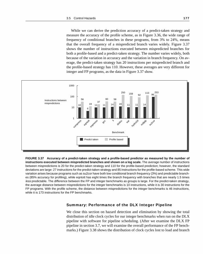
3.5 Control Hazards 177
andge of
eans3.37s for
, bothn av-h andnt for
totalLX
FPnch-anch
While we can derive the prediction accuracy of a predict-taken strategymeasure the accuracy of the profile scheme, as in Figure 3.36, the wide ranfrequency of conditional branches in these programs, from 3% to 24%, mthat the overall frequency of a mispredicted branch varies widely. Figure shows the number of instructions executed between mispredicted brancheboth a profile-based and a predict-taken strategy. The number varies widelybecause of the variation in accuracy and the variation in branch frequency. Oerage, the predict-taken strategy has 20 instructions per mispredicted brancthe profile-based strategy has 110. However, these averages are very differeinteger and FP programs, as the data in Figure 3.37 show.
Summary: Performance of the DLX Integer Pipeline
We close this section on hazard detection and elimination by showing the distribution of idle clock cycles for our integer benchmarks when run on the Dpipeline with software for pipeline scheduling. (After we examine the DLX pipeline in section 3.7, we will examine the overall performance of the FP bemarks.) Figure 3.38 shows the distribution of clock cycles lost to load and br
FIGURE 3.37 Accuracy of a predict-taken strategy and a profile-based predictor as measured by the number ofinstructions executed between mispredicted branches and shown on a log scale. The average number of instructionsbetween mispredictions is 20 for the predict-taken strategy and 110 for the profile-based prediction; however, the standarddeviations are large: 27 instructions for the predict-taken strategy and 85 instructions for the profile-based scheme. This widevariation arises because programs such as su2cor have both low conditional branch frequency (3%) and predictable branch-es (85% accuracy for profiling), while eqntott has eight times the branch frequency with branches that are nearly 1.5 timesless predictable. The difference between the FP and integer benchmarks as groups is large. For the predict-taken strategy,the average distance between mispredictions for the integer benchmarks is 10 instructions, while it is 30 instructions for theFP programs. With the profile scheme, the distance between mispredictions for the integer benchmarks is 46 instructions,while it is 173 instructions for the FP benchmarks.
Instructions betweenmispredictions
1
10
100
1000
11
9692
11
159
19
250
14
58
11
60
1137
6
1910
56
14
113 253
Profile basedPredict taken
Benchmark
com
pres
s
eqnt
ott
espr
esso gc
c li
dodu
cea
r
hydr
o2d
mdlj
dp
su2c
or

178 Chapter 3 Pipelining
n Fig-
r in-fromrfectrfor-
l with con-n or-
iscuss
delays, which is obtained by combining the separate measurements shown iures 3.16 (page 157) and 3.31 (page 171).
Overall the integer programs exhibit an average of 0.06 branch stalls pestruction and 0.05 load stalls per instruction, leading to an average CPI pipelining (i.e., assuming a perfect memory system) of 1.11. Thus, with a pememory system and no clock overhead, pipelining could improve the pemance of these five integer SPECint92 benchmarks by 5/1.11 or 4.5 times.
Now that we understand how to detect and resolve hazards, we can deasome complications that we have avoided so far. The first part of this sectionsiders the challenges of exceptional situations where the instruction executioder is changed in unexpected ways. In the second part of this section, we dsome of the challenges raised by different instruction sets.
FIGURE 3.38 Percentage of the instructions that cause a stall cycle. This assumes aperfect memory system; the clock-cycle count and instruction count would be identical if therewere no integer pipeline stalls. It also assumes the availability of both a basic delayed branchand a cancelling delayed branch, both with one cycle of delay. According to the graph, from8% to 23% of the instructions cause a stall (or a cancelled instruction), leading to CPIs frompipeline stalls that range from 1.09 to 1.23. The pipeline scheduler fills load delays beforebranch delays, and this affects the distribution of delay cycles.
3.6 What Makes Pipelining Hard to Implement?
Percentage of all instructions that stall
0%
2%
4%
6%
8%
10%
12%
14%
5%
7%
3%
9%
14%
4%5%
4%5%
7%
Load stallsBranch stalls
Benchmark
com
pres
s
eqnt
ott
espr
esso gc
c li

3.6 What Makes Pipelining Hard to Implement? 179
e theuc-n in-
ycles.maylete.nder- exist
xecu-
term
se agureents
lin thesemi-
Dealing with Exceptions
Exceptional situations are harder to handle in a pipelined machine becausoverlapping of instructions makes it more difficult to know whether an instrtion can safely change the state of the machine. In a pipelined machine, astruction is executed piece by piece and is not completed for several clock cUnfortunately, other instructions in the pipeline can raise exceptions that force the machine to abort the instructions in the pipeline before they compBefore we discuss these problems and their solutions in detail, we need to ustand what types of situations can arise and what architectural requirementsfor supporting them.
Types of Exceptions and RequirementsThe terminology used to describe exceptional situations where the normal etion order of instruction is changed varies among machines. The terms interrupt,fault, and exception are used, though not in a consistent fashion. We use the exception to cover all these mechanisms, including the following:
I/O device request
Invoking an operating system service from a user program
Tracing instruction execution
Breakpoint (programmer-requested interrupt)
Integer arithmetic overflow
FP arithmetic anomaly (see Appendix A)
Page fault (not in main memory)
Misaligned memory accesses (if alignment is required)
Memory-protection violation
Using an undefined or unimplemented instruction
Hardware malfunctions
Power failure
When we wish to refer to some particular class of such exceptions, we will ulonger name, such as I/O interrupt, floating-point exception, or page fault. Fi3.39 shows the variety of different names for the common exception evabove.
Although we use the name exception to cover all of these events, individuaevents have important characteristics that determine what action is needed hardware.The requirements on exceptions can be characterized on five independent axes:

180 Chapter 3 Pipelining
v-tion,
mory.f the
1. Synchronous versus asynchronous—If the event occurs at the same place eery time the program is executed with the same data and memory allocathe event is synchronous. With the exception of hardware malfunctions, asyn-chronous events are caused by devices external to the processor and meAsynchronous events usually can be handled after the completion ocurrent instruction, which makes them easier to handle.
Exception event IBM 360 VAX Motorola 680x0 Intel 80x86
I/O device request Input/output interruption
Device interrupt Exception (Level 0...7 autovector)
Vectored interrupt
Invoking the operat-ing system service from a user program
Supervisor call interruption
Exception (change mode supervisor trap)
Exception (unimplemented instruction)—on Macintosh
Interrupt (INT instruction)
Tracing instruction execution
Not applicable Exception (trace fault)
Exception (trace) Interrupt (single-step trap)
Breakpoint Not applicable Exception (break-point fault)
Exception (illegal instruction or break-point)
Interrupt (break-point trap)
Integer arithmetic overflow or under-flow; FP trap
Program interrup-tion (overflow or underflow exception)
Exception (integer overflow trap or floating underflow fault)
Exception (floating-point coprocessor errors)
Interrupt (overflow trap or math unit exception)
Page fault (not in main memory)
Not applicable (only in 370)
Exception (transla-tion not valid fault)
Exception (memory-management unit errors)
Interrupt (page fault)
Misaligned memory accesses
Program interrup-tion (specification exception)
Not applicable Exception (address error)
Not applicable
Memory protection violations
Program interrup-tion (protection exception)
Exception (access control violation fault)
Exception (bus error)
Interrupt (protection exception)
Using undefined instructions
Program interrup-tion (operation exception)
Exception (opcode privileged/reserved fault)
Exception (illegal instruction or break-point/unimplemented instruction)
Interrupt (invalid opcode)
Hardware malfunctions
Machine-check interruption
Exception (machine-check abort)
Exception (bus error)
Not applicable
Power failure Machine-check interruption
Urgent interrupt Not applicable Nonmaskable interrupt
FIGURE 3.39 The names of common exceptions vary across four different architectures. Every event on the IBM360 and 80x86 is called an interrupt, while every event on the 680x0 is called an exception. VAX divides events into inter-rupts or exceptions. Adjectives device, software, and urgent are used with VAX interrupts, while VAX exceptions are subdi-vided into faults, traps, and aborts.

3.6 What Makes Pipelining Hard to Implement? 181
xcep-r, be-
are usedctionptions
userre not
-r
rxe-
e thatctionin in- and
eerattion of
fiveuc-s re-
cutinge pro-s pro-idesestartid tokedipe-
2. User requested versus coerced—If the user task directly asks for it, it is a user-request event. In some sense, user-requested exceptions are not really etions, since they are predictable. They are treated as exceptions, howevecause the same mechanisms that are used to save and restore the state for these user-requested events. Because the only function of an instruthat triggers this exception is to cause the exception, user-requested excecan always be handled after the instruction has completed. Coerced exceptionsare caused by some hardware event that is not under the control of theprogram. Coerced exceptions are harder to implement because they apredictable.
3. User maskable versus user nonmaskable—If an event can be masked or disabled by a user task, it is user maskable. This mask simply controls whethethe hardware responds to the exception or not.
4. Within versus between instructions—This classification depends on whethethe event prevents instruction completion by occurring in the middle of ecution—no matter how short—or whether it is recognized between instruc-tions. Exceptions that occur within instructions are usually synchronous, sincthe instruction triggers the exception. It’s harder to implement exceptionsoccur within instructions than those between instructions, since the instrumust be stopped and restarted. Asynchronous exceptions that occur withstructions arise from catastrophic situations (e.g., hardware malfunction)always cause program termination.
5. Resume versus terminate—If the program’s execution always stops after thinterrupt, it is a terminating event. If the program’s execution continues aftthe interrupt, it is a resuming event. It is easier to implement exceptions thterminate execution, since the machine need not be able to restart executhe same program after handling the exception.
Figure 3.40 classifies the examples from Figure 3.39 according to thesecategories. The difficult task is implementing interrupts occurring within instrtions where the instruction must be resumed. Implementing such exceptionquires that another program must be invoked to save the state of the exeprogram, correct the cause of the exception, and then restore the state of thgram before the instruction that caused the exception can be tried again. Thicess must be effectively invisible to the executing program. If a pipeline provthe ability for the machine to handle the exception, save the state, and rwithout affecting the execution of the program, the pipeline or machine is sabe restartable. While early supercomputers and microprocessors often lacthis property, almost all machines today support it, at least for the integer pline, because it is needed to implement virtual memory (see Chapter 5).

182 Chapter 3 Pipelining
rop-tione re-ult- theexe-othery shutorrectn at
inueshion.ondi-cep-eline
e
te
e
Stopping and Restarting ExecutionAs in unpipelined implementations, the most difficult exceptions have two perties: (1) they occur within instructions (that is, in the middle of the instrucexecution corresponding to EX or MEM pipe stages), and (2) they must bstartable. In our DLX pipeline, for example, a virtual memory page fault resing from a data fetch cannot occur until sometime in the MEM stage ofinstruction. By the time that fault is seen, several other instructions will be in cution. A page fault must be restartable and requires the intervention of anprocess, such as the operating system. Thus, the pipeline must be safeldown and the state saved so that the instruction can be restarted in the cstate. Restarting is usually implemented by saving the PC of the instructiowhich to restart. If the restarted instruction is not a branch, then we will contto fetch the sequential successors and begin their execution in the normal faIf the restarted instruction is a branch, then we will reevaluate the branch ction and begin fetching from either the target or the fall through. When an extion occurs, the pipeline control can take the following steps to save the pipstate safely:
Exception typeSynchronous vs. asynchronous
User request vs. coerced
User maskable vs. nonmaskable
Within vs. betweeninstructions
Resume vs. terminate
I/O device request Asynchronous Coerced Nonmaskable Between Resume
Invoke operating system Synchronous User request
Nonmaskable Between Resume
Tracing instruction execution Synchronous User request
User maskable Between Resume
Breakpoint Synchronous User request
User maskable Between Resume
Integer arithmetic overflow Synchronous Coerced User maskable Within Resume
Floating-point arithmetic overflow or underflow
Synchronous Coerced User maskable Within Resume
Page fault Synchronous Coerced Nonmaskable Within Resume
Misaligned memory accesses Synchronous Coerced User maskable Within Resum
Memory-protection violations
Synchronous Coerced Nonmaskable Within Resume
Using undefined instructions Synchronous Coerced Nonmaskable Within Termina
Hardware malfunctions Asynchronous Coerced Nonmaskable Within Terminat
Power failure Asynchronous Coerced Nonmaskable Within Terminate
FIGURE 3.40 Five categories are used to define what actions are needed for the different exception types shownin Figure 3.39. Exceptions that must allow resumption are marked as resume, although the software may often choose toterminate the program. Synchronous, coerced exceptions occurring within instructions that can be resumed are the mostdifficult to implement. We might expect that memory protection access violations would always result in termination; how-ever, modern operating systems use memory protection to detect events such as the first attempt to use a page or the firstwrite to a page. Thus, processors should be able to resume after such exceptions.

3.6 What Makes Pipelining Hard to Implement? 183
allintouc-ction.d be-
trol,sed
long-the in-e andone in
chine (us-
in-t can
dlingotheromees, theination mayrit-pera-igh-e hasourse,ting-
064,mes)
oth-At alerstwareasier,cise
1. Force a trap instruction into the pipeline on the next IF.
2. Until the trap is taken, turn off all writes for the faulting instruction and forinstructions that follow in the pipeline; this can be done by placing zeros the pipeline latches of all instructions in the pipeline, starting with the instrtion that generates the exception, but not those that precede that instruThis prevents any state changes for instructions that will not be completefore the exception is handled.
3. After the exception-handling routine in the operating system receives conit immediately saves the PC of the faulting instruction. This value will be uto return from the exception later.
When we use delayed branches, as mentioned in the last section, it is noer possible to re-create the state of the machine with a single PC because structions in the pipeline may not be sequentially related. So we need to savrestore as many PCs as the length of the branch delay plus one. This is dthe third step above.
After the exception has been handled, special instructions return the mafrom the exception by reloading the PCs and restarting the instruction streaming the instruction RFE in DLX). If the pipeline can be stopped so that thestructions just before the faulting instruction are completed and those after ibe restarted from scratch, the pipeline is said to have precise exceptions. Ideally,the faulting instruction would not have changed the state, and correctly hansome exceptions requires that the faulting instruction have no effects. For exceptions, such as floating-point exceptions, the faulting instruction on smachines writes its result before the exception can be handled. In such cashardware must be prepared to retrieve the source operands, even if the destis identical to one of the source operands. Because floating-point operationsrun for many cycles, it is highly likely that some other instruction may have wten the source operands (as we will see in the next section, floating-point otions often complete out of order). To overcome this, many recent hperformance machines have introduced two modes of operation. One modprecise exceptions and the other (fast or performance mode) does not. Of cthe precise exception mode is slower, since it allows less overlap among floapoint instructions. In some high-performance machines, including Alpha 21Power-2, and MIPS R8000, the precise mode is often much slower (>10 tiand thus useful only for debugging of codes.
Supporting precise exceptions is a requirement in many systems, while iners it is “just” valuable because it simplifies the operating system interface. minimum, any machine with demand paging or IEEE arithmetic trap handmust make its exceptions precise, either in the hardware or with some sofsupport. For integer pipelines, the task of creating precise exceptions is eand accommodating virtual memory strongly motivates the support of pre

184 Chapter 3 Pipelining
ignerse. Ininte-hal-
ons thexam-
ption
d thenst, ifndled
Ex-ptione of in-heen
;
exceptions for memory references. In practice, these reasons have led desand architects to always provide precise exceptions for the integer pipelinthis section we describe how to implement precise exceptions for the DLX ger pipeline. We will describe techniques for handling the more complex clenges arising in the FP pipeline in section 3.7.
Exceptions in DLX
Figure 3.41 shows the DLX pipeline stages and which “problem” exceptimight occur in each stage. With pipelining, multiple exceptions may occur insame clock cycle because there are multiple instructions in execution. For eple, consider this instruction sequence:
This pair of instructions can cause a data page fault and an arithmetic exceat the same time, since the LW is in the MEM stage while the ADD is in the EXstage. This case can be handled by dealing with only the data page fault anrestarting the execution. The second exception will reoccur (but not the firthe software is correct), and when the second exception occurs, it can be haindependently.
In reality, the situation is not as straightforward as this simple example.ceptions may occur out of order; that is, an instruction may cause an excebefore an earlier instruction causes one. Consider again the above sequencstructions, LW followed by ADD. The LW can get a data page fault, seen when tinstruction is in MEM, and the ADD can get an instruction page fault, seen wh
LW IF ID EX MEM WB
ADD IF ID EX MEM WB
Pipeline stage Problem exceptions occurring
IF Page fault on instruction fetch; misaligned memory accessmemory-protection violation
ID Undefined or illegal opcode
EX Arithmetic exception
MEM Page fault on data fetch; misaligned memory access;memory-protection violation
WB None
FIGURE 3.41 Exceptions that may occur in the DLX pipeline. Exceptions raised from in-struction or data-memory access account for six out of eight cases.

3.6 What Makes Pipelining Hard to Implement? 185
t,
han-,
n out by a
ptionce anl thatister
MEM,es an
tatusder inrre-
at in-n onelesee in
xcep-ns.
thatuar-
ng ofxcep- stateces-modesecu-t willd thecise
af-at-
stly,
the ADD instruction is in IF. The instruction page fault will actually occur firseven though it is caused by a later instruction!
Since we are implementing precise exceptions, the pipeline is required todle the exception caused by the LW instruction first. To explain how this workslet’s call the instruction in the position of the LW instruction i, and the instructionin the position of the ADD instruction i + 1. The pipeline cannot simply handle aexception when it occurs in time, since that will lead to exceptions occurringof the unpipelined order. Instead, the hardware posts all exceptions causedgiven instruction in a status vector associated with that instruction. The excestatus vector is carried along as the instruction goes down the pipeline. Onexception indication is set in the exception status vector, any control signamay cause a data value to be written is turned off (this includes both regwrites and memory writes). Because a store can cause an exception during the hardware must be prepared to prevent the store from completing if it raisexception.
When an instruction enters WB (or is about to leave MEM), the exception svector is checked. If any exceptions are posted, they are handled in the orwhich they would occur in time on an unpipelined machine—the exception cosponding to the earliest instruction (and usually the earliest pipe stage for thstruction) is handled first. This guarantees that all exceptions will be seeinstruction i before any are seen on i + 1. Of course, any action taken in earlier pipstages on behalf of instruction i may be invalid, but since writes to the register fiand memory were disabled, no state could have been changed. As we will section 3.7, maintaining this precise model for FP operations is much harder.
In the next subsection we describe problems that arise in implementing etions in the pipelines of machines with more powerful, longer-running instructio
Instruction Set Complications
No DLX instruction has more than one result, and our DLX pipeline writes result only at the end of an instruction’s execution. When an instruction is ganteed to complete it is called committed. In the DLX integer pipeline, all instruc-tions are committed when they reach the end of the MEM stage (or beginniWB) and no instruction updates the state before that stage. Thus, precise etions are straightforward. Some machines have instructions that change thein the middle of the instruction execution, before the instruction and its predesors are guaranteed to complete. For example, autoincrement addressing on the VAX cause the update of registers in the middle of an instruction extion. In such a case, if the instruction is aborted because of an exception, ileave the machine state altered. Although we know which instruction causeexception, without additional hardware support the exception will be imprebecause the instruction will be half finished. Restarting the instruction streamter such an imprecise exception is difficult. Alternatively, we could avoid upding the state before the instruction commits, but this may be difficult or co

186 Chapter 3 Pipelining
uctionecisebackption
valueat andption
ory0. Tore de-tate ofd onntin-rtedchine
le ofrkingstate of
ddi-ondi-odes
ondi-ow-
anyst in-tween
cidetionth im-lua-e. be-ntrol the
as anst as
to
since there may be dependences on the updated state: Consider a VAX instrthat autoincrements the same register multiple times. Thus, to maintain a prexception model, most machines with such instructions have the ability to out any state changes made before the instruction is committed. If an exceoccurs, the machine uses this ability to reset the state of the machine to itsbefore the interrupted instruction started. In the next section, we will see thmore powerful DLX floating-point pipeline can introduce similar problems, athe next chapter introduces techniques that substantially complicate excehandling.
A related source of difficulties arises from instructions that update memstate during execution, such as the string copy operations on the VAX or 36make it possible to interrupt and restart these instructions, the instructions afined to use the general-purpose registers as working registers. Thus the sthe partially completed instruction is always in the registers, which are savean exception and restored after the exception, allowing the instruction to coue. In the VAX an additional bit of state records when an instruction has staupdating the memory state, so that when the pipeline is restarted, the maknows whether to restart the instruction from the beginning or from the middthe instruction. The 80x86 string instructions also use the registers as wostorage, so that saving and restoring the registers saves and restores the such instructions.
A different set of difficulties arises from odd bits of state that may create ational pipeline hazards or may require extra hardware to save and restore. Ction codes are a good example of this. Many machines set the condition cimplicitly as part of the instruction. This approach has advantages, since ction codes decouple the evaluation of the condition from the actual branch. Hever, implicitly set condition codes can cause difficulties in scheduling pipeline delays between setting the condition code and the branch, since mostructions set the condition code and cannot be used in the delay slots bethe condition evaluation and the branch.
Additionally, in machines with condition codes, the processor must dewhen the branch condition is fixed. This involves finding out when the condicode has been set for the last time before the branch. In most machines wiplicitly set condition codes, this is done by delaying the branch condition evation until all previous instructions have had a chance to set the condition cod
Of course, architectures with explicitly set condition codes allow the delaytween condition test and the branch to be scheduled; however, pipeline comust still track the last instruction that sets the condition code to know whenbranch condition is decided. In effect, the condition code must be treated operand that requires hazard detection for RAW hazards with branches, juDLX must do on the registers.
A final thorny area in pipelining is multicycle operations. Imagine tryingpipeline a sequence of VAX instructions such as this:

3.7 Extending the DLX Pipeline to Handle Multicycle Operations 187
ire,rent
ta haz- sim-lockds andX at00
ctionthecanuch
ilarships for
ine
ting-ign al-
point
ink, or, thesi-
pipe-ycleumbertipleed data
MOVL R1,R2
ADDL3 42(R1),56(R1)+,@(R1)
SUBL2 R2,R3
MOVC3 @(R1)[R2],74(R2),R3
These instructions differ radically in the number of clock cycles they will requfrom as low as one up to hundreds of clock cycles. They also require diffenumbers of data memory accesses, from zero to possibly hundreds. The daards are very complex and occur both between and within instructions. Theple solution of making all instructions execute for the same number of ccycles is unacceptable, because it introduces an enormous number of hazarbypass conditions and makes an immensely long pipeline. Pipelining the VAthe instruction level is difficult, but a clever solution was found by the VAX 88designers. They pipeline the microinstruction execution: a microinstruction is asimple instruction used in sequences to implement a more complex instruset. Because the microinstructions are simple (they look a lot like DLX), pipeline control is much easier. While it is not clear that this approach achieve quite as low a CPI as an instruction-level pipeline for the VAX, it is msimpler, possibly leading to a shorter clock cycle.
In comparison, load-store machines have simple operations with simamounts of work and pipeline more easily. If architects realize the relationbetween instruction set design and pipelining, they can design architecturemore efficient pipelining. In the next section we will see how the DLX pipeldeals with long-running instructions, specifically floating-point operations.
We now want to explore how our DLX pipeline can be extended to handle floapoint operations. This section concentrates on the basic approach and the desternatives, closing with some performance measurements of a DLX floating-pipeline.
It is impractical to require that all DLX floating-point operations completeone clock cycle, or even in two. Doing so would mean accepting a slow clocusing enormous amounts of logic in the floating-point units, or both. Insteadfloating-point pipeline will allow for a longer latency for operations. This is eaer to grasp if we imagine the floating-point instructions as having the same line as the integer instructions, with two important changes. First, the EX cmay be repeated as many times as needed to complete the operation—the nof repetitions can vary for different operations. Second, there may be mulfloating-point functional units. A stall will occur if the instruction to be issuwill either cause a structural hazard for the functional unit it uses or cause ahazard.
3.7 Extending the DLX Pipeline toHandle Multicycle Operations

188 Chapter 3 Pipelining
its in
tions,
t pipe-s notpre- EX
unitf clockwn in
For this section, let’s assume that there are four separate functional unour DLX implementation:
1. The main integer unit that handles loads and stores, integer ALU operaand branches.
2. FP and integer multiplier.
3. FP adder that handles FP add, subtract, and conversion.
4. FP and integer divider.
If we also assume that the execution stages of these functional units are nolined, then Figure 3.42 shows the resulting pipeline structure. Because EX ipipelined, no other instruction using that functional unit may issue until the vious instruction leaves EX. Moreover, if an instruction cannot proceed to thestage, the entire pipeline behind that instruction will be stalled.
In reality, the intermediate results are probably not cycled around the EXas Figure 3.42 suggests; instead, the EX pipeline stage has some number odelays larger than 1. We can generalize the structure of the FP pipeline sho
FIGURE 3.42 The DLX pipeline with three additional unpipelined, floating-point, func-tional units. Because only one instruction issues on every clock cycle, all instructions gothrough the standard pipeline for integer operations. The floating-point operations simply loopwhen they reach the EX stage. After they have finished the EX stage, they proceed to MEMand WB to complete execution.
EX
FP/integermultiply
EX
Integer unit
EX
FP adder
EX
FP/integerdivider
IF ID MEM WB

3.7 Extending the DLX Pipeline to Handle Multicycle Operations 189
ons.ional
n in-initia-suingitia-
0,ncy ofpera-
y theple,
ion istencyill be
n thetagebove,n FP
r log-ed forlong-
ding 3.44inter-hichepen-clockthose active.
Figure 3.42 to allow pipelining of some stages and multiple ongoing operatiTo describe such a pipeline, we must define both the latency of the functunits and also the initiation interval or repeat interval. We define latency thesame way we defined it earlier: the number of intervening cycles between astruction that produces a result and an instruction that uses the result. The tion or repeat interval is the number of cycles that must elapse between istwo operations of a given type. For example, we will use the latencies and intion intervals shown in Figure 3.43.
With this definition of latency, integer ALU operations have a latency ofsince the results can be used on the next clock cycle, and loads have a late1, since their results can be used after one intervening cycle. Since most otions consume their operands at the beginning of EX, the latency is usuallnumber of stages after EX that an instruction produces a result—for examzero stages for ALU operations and one stage for loads. The primary exceptstores, which consume the value being stored one cycle later. Hence the lato a store for the value being stored, but not for the base address register, wone cycle less. Pipeline latency is essentially equal to one cycle less thadepth of the execution pipeline, which is the number of stages from the EX sto the stage that produces the result. Thus, for the example pipeline just athe number of stages in an FP add is four, while the number of stages in amultiply is seven. To achieve a higher clock rate, designers need to put feweic levels in each pipe stage, which makes the number of pipe stages requirmore complex operations larger. The penalty for the faster clock rate is thus er latency for operations.
The example pipeline structure in Figure 3.43 allows up to four outstanFP adds, seven outstanding FP/integer multiplies, and one FP divide. Figureshows how this pipeline can be drawn by extending Figure 3.42. The repeat val is implemented in Figure 3.44 by adding additional pipeline stages, wwill be separated by additional pipeline registers. Because the units are inddent, we name the stages differently. The pipeline stages that take multiple cycles, such as the divide unit, are further subdivided to show the latency of stages. Because they are not complete stages, only one operation may be
Functional unit Latency Initiation interval
Integer ALU 0 1
Data memory (integer and FP loads) 1 1
FP add 3 1
FP multiply (also integer multiply) 6 1
FP divide (also integer divide) 24 25
FIGURE 3.43 Latencies and initiation intervals for functional units.

190 Chapter 3 Pipelining
arliernd FP
es thetion.
The pipeline structure can also be shown using the familiar diagrams from ein the chapter, as Figure 3.45 shows for a set of independent FP operations aloads and stores. Naturally, the longer latency of the FP operations increasfrequency of RAW hazards and resultant stalls, as we will see later in this sec
FIGURE 3.44 A pipeline that supports multiple outstanding FP operations. The FP multiplier and adder are fully pipe-lined and have a depth of seven and four stages, respectively. The FP divider is not pipelined, but requires 24 clock cyclesto complete. The latency in instructions between the issue of an FP operation and the use of the result of that operationwithout incurring a RAW stall is determined by the number of cycles spent in the execution stages. For example, the fourthinstruction after an FP add can use the result of the FP add. For integer ALU operations, the depth of the execution pipelineis always one and the next instruction can use the results. Both FP loads and integer loads complete during MEM, whichmeans that the memory system must provide either 32 or 64 bits in a single clock.
MULTD IF ID M1 M2 M3 M4 M5 M6 M7 MEM WB
ADDD IF ID A1 A2 A3 A4 MEM WB
LD IF ID EX MEM WB
SD IF ID EX MEM WB
FIGURE 3.45 The pipeline timing of a set of independent FP operations. The stages in italics show where data isneeded, while the stages in bold show where a result is available. FP loads and stores use a 64-bit path to memory so thatthe pipelining timing is just like an integer load or store.
EX
M1
FP/integer multiply
Integer unit
FP adder
FP/integer divider
IF ID MEM WB
M2 M3 M4 M5 M6
A1 A2 A3 A4
M7
DIV

3.7 Extending the DLX Pipeline to Handle Multicycle Operations 191
ad-of con-so-orught
parateontrol
rding
cur.lled.
ister
Note ID.
using
ore
y the that
l im-he re-s FP
the of FPnflicts
3.47:gis- thezard.mayis isad, we
The structure of the pipeline in Figure 3.44 requires the introduction of theditional pipeline registers (e.g., A1/A2, A2/A3, A3/A4) and the modification the connections to those registers. The ID/EX register must be expanded tonect ID to EX, DIV, M1, and A1; we can refer to the portion of the register asciated with one of the next stages with the notation ID/EX, ID/DIV, ID/M1, ID/A1. The pipeline register between ID and all the other stages may be thoof as logically separate registers and may, in fact, be implemented as seregisters. Because only one operation can be in a pipe stage at a time, the cinformation can be associated with the register at the head of the stage.
Hazards and Forwarding in Longer Latency Pipelines
There are a number of different aspects to the hazard detection and forwafor a pipeline like that in Figure 3.44:
1. Because the divide unit is not fully pipelined, structural hazards can ocThese will need to be detected and issuing instructions will need to be sta
2. Because the instructions have varying running times, the number of regwrites required in a cycle can be larger than 1.
3. WAW hazards are possible, since instructions no longer reach WB in order.that WAR hazards are not possible, since the register reads always occur in
4. Instructions can complete in a different order than they were issued, caproblems with exceptions; we deal with this in the next subsection.
5. Because of longer latency of operations, stalls for RAW hazards will be mfrequent.
The increase in stalls arising from longer operation latencies is fundamentallsame as that for the integer pipeline. Before describing the new problemsarise in this FP pipeline and looking at solutions, let’s examine the potentiapact of RAW hazards. Figure 3.46 shows a typical FP code sequence and tsultant stalls. At the end of this section, we’ll examine the performance of thipipeline for our SPEC subset.
Now look at the problems arising from writes, described as (2) and (3) inlist above. If we assume the FP register file has one write port, sequencesoperations, as well as an FP load together with FP operations, can cause cofor the register write port. Consider the pipeline sequence shown in Figure In clock cycle 11, all three instructions will reach WB and want to write the reter file. With only a single register file write port, the machine must serializeinstruction completion. This single register port represents a structural haWe could increase the number of write ports to solve this, but that solution be unattractive since the additional write ports would be used only rarely. Thbecause the maximum steady state number of write ports needed is 1. Instechoose to detect and enforce access to the write port as a structural hazard.

192 Chapter 3 Pipelining
acksues,
ritetruc-
r filetalledple-ction reg-tion.ntertil
There are two different ways to implement this interlock. The first is to trthe use of the write port in the ID stage and to stall an instruction before it isjust as we would for any other structural hazard. Tracking the use of the wport can be done with a shift register that indicates when already-issued instions will use the register file. If the instruction in ID needs to use the registeat the same time as an instruction already issued, the instruction in ID is sfor a cycle. On each clock the reservation register is shifted one bit. This immentation has an advantage: It maintains the property that all interlock deteand stall insertion occurs in the ID stage. The cost is the addition of the shiftister and write conflict logic. We will assume this scheme throughout this sec
An alternative scheme is to stall a conflicting instruction when it tries to eeither the MEM or WB stage. If we wait to stall the conflicting instructions un
Clock cycle number
Instruction 1 2 3 4 5 6 7 8 9 10 11 12 13 14 15 16 17
LD F4,0(R2)
IF ID EX MEM WB
MULTD F0,F4,F6
IF ID stall M1 M2 M3 M4 M5 M6 M7 MEM WB
ADDD F2,F0,F8
IF stall ID stall stall stall stall stall stall A1 A2 A3 A4 MEM
SD 0(R2),F2
IF stall stall stall stall stall stall ID EX stall stall stall MEM
FIGURE 3.46 A typical FP code sequence showing the stalls arising from RAW hazards. The longer pipeline sub-stantially raises the frequency of stalls versus the shallower integer pipeline. Each instruction in this sequence is dependenton the previous and proceeds as soon as data are available, which assumes the pipeline has full bypassing and forwarding.The SD must be stalled an extra cycle so that its MEM does not conflict with the ADDD. Extra hardware could easily handlethis case.
Clock cycle number
Instruction 1 2 3 4 5 6 7 8 9 10 11
MULTD F0,F4,F6 IF ID M1 M2 M3 M4 M5 M6 M7 MEM WB
... IF ID EX MEM WB
... IF ID EX MEM WB
ADDD F2,F4,F6 IF ID A1 A2 A3 A4 MEM WB
... IF ID EX MEM WB
... IF ID EX MEM WB
LD F2,0(R2) IF ID EX MEM WB
FIGURE 3.47 Three instructions want to perform a write back to the FP register file simultaneously, as shown inclock cycle 11. This is not the worst case, since an earlier divide in the FP unit could also finish on the same clock. Notethat although the MULTD, ADDD, and LD all are in the MEM stage in clock cycle 10, only the LD actually uses the memory,so no structural hazard exists for MEM.

3.7 Extending the DLX Pipeline to Handle Multicycle Operations 193
truc-thed an-me isM orpelinenter- these
xist,
use its
n ae that in
ch is
-
canected
t po-g ID
ue thecanple-
P in-struc-ntegerters,, wezards anting- with-
they want to enter the MEM or WB stage, we can choose to stall either instion. A simple, though sometimes suboptimal, heuristic is to give priority to unit with the longest latency, since that is the one most likely to have causeother instruction to be stalled for a RAW hazard. The advantage of this schethat it does not require us to detect the conflict until the entrance of the MEWB stage, where it is easy to see. The disadvantage is that it complicates picontrol, as stalls can now arise from two places. Notice that stalling before eing MEM will cause the EX, A4, or M7 stage to be occupied, possibly forcingstall to trickle back in the pipeline. Likewise, stalling before WB would cauMEM to back up.
Our other problem is the possibility of WAW hazards. To see that these econsider the example in Figure 3.47. If the LD instruction were issued one cycleearlier and had a destination of F2, then it would create a WAW hazard, becawould write F2 one cycle earlier than the ADDD. Note that this hazard only occurwhen the result of the ADDD is overwritten without any instruction ever using it! Ifthere were a use of F2 between the ADDD and the LD, the pipeline would need tobe stalled for a RAW hazard, and the LD would not issue until the ADDD was com-pleted. We could argue that, for our pipeline, WAW hazards only occur wheuseless instruction is executed, but we must still detect them and make surthe result of the LD appears in F2 when we are done. (As we will seesection 3.10, such sequences sometimes do occur in reasonable code.)
There are two possible ways to handle this WAW hazard. The first approato delay the issue of the load instruction until the ADDD enters MEM. The secondapproach is to stamp out the result of the ADDD by detecting the hazard and changing the control so that the ADDD does not write its result. Then, the LD can issueright away. Because this hazard is rare, either scheme will work fine—youpick whatever is simpler to implement. In either case, the hazard can be detduring ID when the LD is issuing. Then stalling the LD or making the ADDD a no-op is easy. The difficult situation is to detect that the LD might finish before theADDD, because that requires knowing the length of the pipeline and the currensition of the ADDD. Luckily, this code sequence (two writes with no interveninread) will be very rare, so we can use a simple solution: If an instruction inwants to write the same register as an instruction already issued, do not issinstruction to EX. In the next chapter, we will see how additional hardware eliminate stalls for such hazards. First, let’s put together the pieces for immenting the hazard and issue logic in our FP pipeline.
In detecting the possible hazards, we must consider hazards among Fstructions, as well as hazards between an FP instruction and an integer intion. Except for FP loads-stores and FP-integer register moves, the FP and iregisters are distinct. All integer instructions operate on the integer regiswhile the floating-point operations operate only on their own registers. Thusneed only consider FP loads-stores and FP register moves in detecting habetween FP and integer instructions. This simplification of pipeline control isadditional advantage of having separate register files for integer and floapoint data. (The main advantages are a doubling of the number of registers,
194 Chapter 3 Pipelining
moregister
sets.)hecks
tister
dhen
e, de-t willalue
urce/A3, in-
f IDthe caset ig-
ll the
era-is truethe
ion.e the log-
ha-
ated
out making either set larger, and an increase in bandwidth without adding ports to either set. The main disadvantage, beyond the need for an extra refile, is the small cost of occasional moves needed between the two registerAssuming that the pipeline does all hazard detection in ID, there are three cthat must be performed before an instruction can issue:
1. Check for structural hazards—Wait until the required functional unit is nobusy (this is only needed for divides in this pipeline) and make sure the regwrite port is available when it will be needed.
2. Check for a RAW data hazard—Wait until the source registers are not listeas pending destinations in a pipeline register that will not be available wthis instruction needs the result. A number of checks must be made herpending on both the source instruction, which determines when the resulbe available, and the destination instruction, which determines when the vis needed. For example, if the instruction in ID is an FP operation with soregister F2, then F2 cannot be listed as a destination in ID/A1, A1/A2, or A2which correspond to FP add instructions that will not be finished when thestruction in ID needs a result. (ID/A1 is the portion of the output register othat is sent to A1.) Divide is somewhat more tricky, if we want to allow last few cycles of a divide to be overlapped, since we need to handle thewhen a divide is close to finishing as special. In practice, designers mighnore this optimization in favor of a simpler issue test.
3. Check for a WAW data hazard—Determine if any instruction in A1,..., A4, D,M1,..., M7 has the same register destination as this instruction. If so, staissue of the instruction in ID.
Although the hazard detection is more complex with the multicycle FP options, the concepts are the same as for the DLX integer pipeline. The same for the forwarding logic. The forwarding can be implemented by checking if destination register in any of EX/MEM, A4/MEM, M7/MEM, D/MEM, orMEM/WB registers is one of the source registers of a floating-point instructIf so, the appropriate input multiplexer will have to be enabled so as to choosforwarded data. In the Exercises, you will have the opportunity to specify theic for the RAW and WAW hazard detection as well as for forwarding.
Multicycle FP operations also introduce problems for our exception mecnisms, which we deal with next.
Maintaining Precise Exceptions
Another problem caused by these long-running instructions can be illustrwith the following sequence of code:
DIVF F0,F2,F4
ADDF F10,F10,F8

3.7 Extending the DLX Pipeline to Handle Multicycle Operations 195
obleman in-
ventrder
ap-s weis iscat theld
rderut-of- ex-ed in
or arethisemo-cep-rlier,f ex-
. Then of
over- that theIPS
era- solu-ong. Fur-struc-r of
val-ck ear-
SUBF F12,F12,F14
This code sequence looks straightforward; there are no dependences. A prarises, however, because an instruction issued early may complete after struction issued later. In this example, we can expect ADDF and SUBF to completebefore the DIVF completes. This is called out-of-order completion and is commonin pipelines with long-running operations. Because hazard detection will preany dependence among instructions from being violated, why is out-of-ocompletion a problem? Suppose that the SUBF causes a floating-point arithmeticexception at a point where the ADDF has completed but the DIVF has not. The re-sult will be an imprecise exception, something we are trying to avoid. It maypear that this could be handled by letting the floating-point pipeline drain, ado for the integer pipeline. But the exception may be in a position where thnot possible. For example, if the DIVF decided to take a floating-point-arithmetiexception after the add completed, we could not have a precise exception hardware level. In fact, because the ADDF destroys one of its operands, we counot restore the state to what it was before the DIVF, even with software help.
This problem arises because instructions are completing in a different othan they were issued. There are four possible approaches to dealing with oorder completion. The first is to ignore the problem and settle for impreciseceptions. This approach was used in the 1960s and early 1970s. It is still ussome supercomputers, where certain classes of exceptions are not allowedhandled by the hardware without stopping the pipeline. It is difficult to use approach in most machines built today because of features such as virtual mry and the IEEE floating-point standard, which essentially require precise extions through a combination of hardware and software. As mentioned easome recent machines have solved this problem by introducing two modes oecution: a fast, but possibly imprecise mode and a slower, precise modeslower precise mode is implemented either with a mode switch or by insertioexplicit instructions that test for FP exceptions. In either case the amount of lap and reordering permitted in the FP pipeline is significantly restricted soeffectively only one FP instruction is active at a time. This solution is used inDEC Alpha 21064 and 21164, in the IBM Power-1 and Power-2, and in the MR8000.
A second approach is to buffer the results of an operation until all the options that were issued earlier are complete. Some machines actually use thistion, but it becomes expensive when the difference in running times amoperations is large, since the number of results to buffer can become largethermore, results from the queue must be bypassed to continue issuing intions while waiting for the longer instruction. This requires a large numbecomparators and a very large multiplexer.
There are two viable variations on this basic approach. The first is a historyfile, used in the CYBER 180/990. The history file keeps track of the original ues of registers. When an exception occurs and the state must be rolled ba
196 Chapter 3 Pipelining
theuto-r ap-themainr file 4.6), Pow-ving
t im- canations
soft-, and:
n.
d.
turn
ofe-rlytant
ntber of. Foruc-ntialf FPver-
con-willption
f theeans
work,
lier than some instruction that completed out of order, the original value ofregister can be restored from the history file. A similar technique is used for aincrement and autodecrement addressing on machines like VAXes. Anotheproach, the future file, proposed by J. Smith and A. Pleszkun [1988], keeps newer value of a register; when all earlier instructions have completed, the register file is updated from the future file. On an exception, the main registehas the precise values for the interrupted state. In the next chapter (sectionwe will see extensions of this idea, which are used in processors such as theerPC 620 and MIPS R10000 to allow overlap and reordering while preserprecise exceptions.
A third technique in use is to allow the exceptions to become somewhaprecise, but to keep enough information so that the trap-handling routinescreate a precise sequence for the exception. This means knowing what operwere in the pipeline and their PCs. Then, after handling the exception, theware finishes any instructions that precede the latest instruction completedthe sequence can restart. Consider the following worst-case code sequence
Instruction1—A long-running instruction that eventually interrupts executio
Instruction2, ..., Instructionn–1—A series of instructions that are not complete
Instructionn—An instruction that is finished.
Given the PCs of all the instructions in the pipeline and the exception rePC, the software can find the state of instruction1 and instructionn. Becauseinstructionn has completed, we will want to restart execution at instructionn+1.After handling the exception, the software must simulate the executioninstruction1, ..., instructionn–1. Then we can return from the exception and rstart at instructionn+1. The complexity of executing these instructions propeby the handler is the major difficulty of this scheme. There is an imporsimplification for simple DLX-like pipelines: If instruction2, ..., instructionnare all integer instructions, then we know that if instructionn has completed, allof instruction2, ..., instructionn–1 have also completed. Thus, only floating-poioperations need to be handled. To make this scheme tractable, the numfloating-point instructions that can be overlapped in execution can be limitedexample, if we only overlap two instructions, then only the interrupting instrtion need be completed by software. This restriction may reduce the potethroughput if the FP pipelines are deep or if there is a significant number ofunctional units. This approach is used in the SPARC architecture to allow olap of floating-point and integer operations.
The final technique is a hybrid scheme that allows the instruction issue totinue only if it is certain that all the instructions before the issuing instruction complete without causing an exception. This guarantees that when an exceoccurs, no instructions after the interrupting one will be completed and all oinstructions before the interrupting one can be completed. This sometimes mstalling the machine to maintain precise exceptions. To make this scheme

3.7 Extending the DLX Pipeline to Handle Multicycle Operations 197
ear-s toIPSr in
turalaz-ll cy- first
P add,k the
unc-
talls stallsating-elaysaries
the floating-point functional units must determine if an exception is possiblely in the EX stage (in the first three clock cycles in the DLX pipeline), so aprevent further instructions from completing. This scheme is used in the MR2000/3000, the R4000, and the Intel Pentium. It is discussed furtheAppendix A.
Performance of a DLX FP Pipeline
The DLX FP pipeline of Figure 3.44 on page 190 can generate both strucstalls for the divide unit and stalls for RAW hazards (it also can have WAW hards, but this rarely occurs in practice). Figure 3.48 shows the number of stacles for each type of floating-point operation on a per instance basis (i.e., thebar for each FP benchmark shows the number of FP result stalls for each Fsubtract, or compare). As we might expect, the stall cycles per operation traclatency of the FP operations, varying from 46% to 59% of the latency of the ftional unit.
Figure 3.49 gives the complete breakdown of integer and floating-point sfor the five FP SPEC benchmarks we are using. There are four classes ofshown: FP result stalls, FP compare stalls, load and branch delays, and flopoint structural delays. The compiler tries to schedule both load and FP dbefore it schedules branch delays. The total number of stalls per instruction vfrom 0.65 to 1.21.

198 Chapter 3 Pipelining
FIGURE 3.48 Stalls per FP operation for each major type of FP operation. Except forthe divide structural hazards, these data do not depend on the frequency of an operation, onlyon its latency and the number of cycles before the result is used. The number of stalls fromRAW hazards roughly tracks the latency of the FP unit. For example, the average number ofstalls per FP add, subtract, or convert is 1.7 cycles, or 56% of the latency (3 cycles). Likewise,the average number of stalls for multiplies and divides are 2.8 and 14.2, respectively, or 46%and 59% of the corresponding latency. Structural hazards for divides are rare, since the di-vide frequency is low.
Number of stalls
0.0 25.05.0 10.0 20.015.0
FP SPECbenchmarks
doduc
ear
hydro2d
mdljdp
su2cor
0.618.6
1.61.5
0.7
0.024.5
2.91.2
2.1
0.00.4
3.22.5
2.3
0.012.4
2.52.0
1.6
2.015.4
3.71.71.7
Compares MultiplyAdd/subtract/convert
Divide structuralDivide
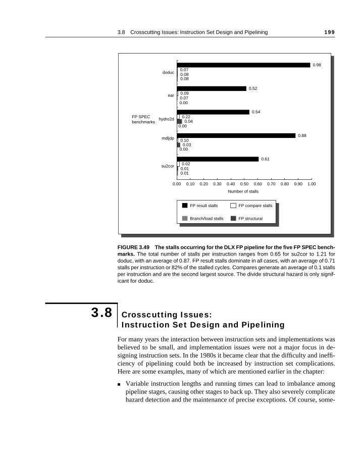
3.8 Crosscutting Issues: Instruction Set Design and Pipelining 199
s wasn de-effi-ns.r:
onglicate
some-
For many years the interaction between instruction sets and implementationbelieved to be small, and implementation issues were not a major focus isigning instruction sets. In the 1980s it became clear that the difficulty and inciency of pipelining could both be increased by instruction set complicatioHere are some examples, many of which are mentioned earlier in the chapte
■ Variable instruction lengths and running times can lead to imbalance ampipeline stages, causing other stages to back up. They also severely comphazard detection and the maintenance of precise exceptions. Of course,
FIGURE 3.49 The stalls occurring for the DLX FP pipeline for the five FP SPEC bench-marks. The total number of stalls per instruction ranges from 0.65 for su2cor to 1.21 fordoduc, with an average of 0.87. FP result stalls dominate in all cases, with an average of 0.71stalls per instruction or 82% of the stalled cycles. Compares generate an average of 0.1 stallsper instruction and are the second largest source. The divide structural hazard is only signif-icant for doduc.
3.8 Crosscutting Issues: Instruction Set Design and Pipelining
Number of stalls
0.00 1.000.200.10 0.40 0.80 0.900.60 0.700.30 0.50
FP SPECbenchmarks
doduc
ear
hydro2d
mdljdp
su2cor
0.010.010.02
0.61
0.000.03
0.100.88
0.000.04
0.220.54
0.000.070.09
0.52
0.080.080.07
0.98
FP compare stalls
FP structural
FP result stalls
Branch/load stalls

200 Chapter 3 Pipelining
causence
ze the ma-x, it
. Ad-plicate re- sub-ine
ingache
r in-truc- thatn in
chrmerdif-ttervery be- (theoth themat-
om- fetch.cond1983]
ouldk cy-
elineinesnedIPSance
times the advantages justify the added complexity. For example, caches instruction running times to vary when they miss; however, the performaadvantages of caches make the added complexity acceptable. To minimicomplexity, most machines freeze the pipeline on a cache miss. Otherchines try to continue running parts of the pipeline; though this is complemay overcome some of the performance losses from cache misses.
■ Sophisticated addressing modes can lead to different sorts of problemsdressing modes that update registers, such as post-autoincrement, comhazard detection. They also slightly increase the complexity of instructionstart. Other addressing modes that require multiple memory accessesstantially complicate pipeline control and make it difficult to keep the pipelflowing smoothly.
■ Architectures that allow writes into the instruction space (self-modifycode), such as the 80x86, can cause trouble for pipelining (as well as for cdesigns). For example, if an instruction in the pipeline can modify anothestruction, we must constantly check if the address being written by an instion corresponds to the address of an instruction following the instructionwrites in the pipeline. If so, the pipeline must be flushed or the instructiothe pipeline somehow updated.
■ Implicitly set condition codes increase the difficulty of finding when a branhas been decided and the difficulty of scheduling branch delays. The foproblem occurs when the condition-code setting is not uniform, making it ficult to decide which instruction assigns the condition code last. The laproblem occurs when the condition code is unconditionally set by almost einstruction. This makes it hard to find instructions that can be scheduledtween the condition evaluation and the branch. Most older architecturesIBM 360, the DEC VAX, and the Intel 80x86, for example) have one or bof these problems. Many newer architectures avoid condition codes or setexplicitly under the control of a bit in the instruction. Either approach dramically reduces pipelining difficulties.
As a simple example, suppose the DLX instruction format were more cplex, so that a separate, decode pipe stage were required before registerThis would increase the branch delay to two clock cycles. At best, the sebranch-delay slot would be wasted at least as often as the first. Gross [found that a second delay slot was only used half as often as the first. This wlead to a performance penalty for the second delay slot of more than 0.1 cloccles per instruction. Another example comes from a comparison of the pipefficiencies of a VAX 8800 and a MIPS R3000. Although these two machhave many similarities in organization, the VAX instruction set was not desigwith pipelining in mind. As a result, on the SPEC89 benchmarks, the MR3000 is faster by between two times and four times, with a mean performadvantage of 2.7 times.

3.9 Putting It All Together: The MIPS R4000 Pipeline 201
IPSple-pipe-epersingarticu-ory
d ver-ns inulti-verycom-
ther
truc-
In this section we look at the pipeline structure and performance of the MR4000 processor family. The MIPS-3 instruction set, which the R4000 imments, is a 64-bit instruction set similar to DLX. The R4000 uses a deeper line than that of our DLX model both for integer and FP programs. This depipeline allows it to achieve higher clock rates (100–200 MHz) by decompothe five-stage integer pipeline into eight stages. Because cache access is plarly time critical, the extra pipeline stages come from decomposing the memaccess. This type of deeper pipelining is sometimes called superpipelining.
Figure 3.50 shows the eight-stage pipeline structure using an abstractesion of the datapath. Figure 3.51 shows the overlap of successive instructiothe pipeline. Notice that although the instruction and data memory occupy mple cycles, they are fully pipelined, so that a new instruction can start on eclock. In fact, the pipeline uses the data before the cache hit detection is plete; Chapter 5 discusses how this can be done in more detail.
The function of each stage is as follows:
■ IF—First half of instruction fetch; PC selection actually happens here, togewith initiation of instruction cache access.
■ IS—Second half of instruction fetch, complete instruction cache access.
■ RF—Instruction decode and register fetch, hazard checking, and also instion cache hit detection.
3.9 Putting It All Together: The MIPS R4000 Pipeline
FIGURE 3.50 The eight-stage pipeline structure of the R4000 uses pipelined instruc-tion and data caches. The pipe stages are labeled and their detailed function is describedin the text. The vertical dashed lines represent the stage boundaries as well as the locationof pipeline latches. The instruction is actually available at the end of IS, but the tag check isdone in RF, while the registers are fetched. Thus, we show the instruction memory as oper-ating through RF. The TC stage is needed for data memory access, since we cannot write thedata into the register until we know whether the cache access was a hit or not.
IF IS
Instruction memory Reg
ALU Data memory Reg
RF EX DF DS TC WB

202 Chapter 3 Pipelining
on,
this 3.51e enddiate- in-
ranch de-g twoimplyy slot
■ EX—Execution, which includes effective address calculation, ALU operatiand branch target computation and condition evaluation.
■ DF—Data fetch, first half of data cache access.
■ DS—Second half of data fetch, completion of data cache access.
■ TC—Tag check, determine whether the data cache access hit.
■ WB—Write back for loads and register-register operations.
In addition to substantially increasing the amount of forwarding required, longer latency pipeline increases both the load and branch delays. Figureshows that load delays are two cycles, since the data value is available at thof DS. Figure 3.52 shows the shorthand pipeline schedule when a use immely follows a load. It shows that forwarding is required for the result of a loadstruction to a destination that is three or four cycles later.
Figure 3.53 shows that the basic branch delay is three cycles, since the bcondition is computed during EX. The MIPS architecture has a single-cyclelayed branch. The R4000 uses a predict-not-taken strategy for the remainincycles of the branch delay. As Figure 3.54 shows, untaken branches are sone-cycle delayed branches, while taken branches have a one-cycle dela
FIGURE 3.51 The structure of the R4000 integer pipeline leads to a two-cycle load delay. A two-cycle delay is pos-sible because the data value is available at the end of DS and can be bypassed. If the tag check in TC indicates a miss, thepipeline is backed up a cycle, when the correct data are available.
CC 1
Time (in clock cycles)
CC 2
Instruction memory Reg
ALU Data memory Reg
Instruction memory Reg
ALU Data memory Reg
Instruction memory Reg
ALU Data memory Reg
Instruction memory
LW R1
Instruction 1
Instruction 2
ADD R2, R1 Reg
ALU Data memory Reg
CC 3 CC 4 CC 5 CC 6 CC 7 CC 8 CC 9 CC 10 CC 11

3.9 Putting It All Together: The MIPS R4000 Pipeline 203
uc-slot.ken
followed by two idle cycles. The instruction set provides a branch likely instrtion, which we described earlier and which helps in filling the branch delay Pipeline interlocks enforce both the two-cycle branch stall penalty on a tabranch and any data hazard stall that arises from use of a load result.
Clock number
Instruction number 1 2 3 4 5 6 7 8 9
LW R1, . . . IF IS RF EX DF DS TC WB
ADD R2,R1, . . . IF IS RF stall stall EX DF DS
SUB R3,R1, . . . IF IS stall stall RF EX DF
OR R4,R1, . . . IF stall stall IS RF EX
FIGURE 3.52 A load instruction followed by an immediate use results in a two-cycle stall. Normal forwarding pathscan be used after two cycles, so the ADD and SUB get the value by forwarding after the stall. The OR instruction gets thevalue from the register file. Since the two instructions after the load could be independent and hence not stall, the bypasscan be to instructions that are three or four cycles after the load.
FIGURE 3.53 The basic branch delay is three cycles, since the condition evaluation is performed during EX.
CC1
Time (in clock cycles)
CC2
Instruction memory Reg
ALU Data memory Reg
Instruction memory Reg
ALU Data memory Reg
Instruction memory Reg
ALU Data memory Reg
Instruction memory
BEQZ
Instruction 1
Instruction 2
Instruction 3
Target
Reg
ALU Data memory Reg
Instruction memory Reg
ALU Data memory
CC3 CC4 CC5 CC6 CC7 CC8 CC9 CC10 CC11

204 Chapter 3 Pipelining
elineLXonse-
/TC,ndi-
oint00,sionfor aTheges,
In addition to the increase in stalls for loads and branches, the deeper pipincreases the number of levels of forwarding for ALU operations. In our Dfive-stage pipeline, forwarding between two register-register ALU instructicould happen from the ALU/MEM or the MEM/WB registers. In the R4000 pipline, there are four possible sources for an ALU bypass: EX/DF, DF/DS, DSand TC/WB. The Exercises ask you to explore all the possible forwarding cotions for the DLX instruction set using an R4000-style pipeline.
The Floating-Point Pipeline
The R4000 floating-point unit consists of three functional units: a floating-pdivider, a floating-point multiplier, and a floating-point adder. As in the R30the adder logic is used on the final step of a multiply or divide. Double-preciFP operations can take from two cycles (for a negate) up to 112 cycles square root. In addition, the various units have different initiation rates. floating-point functional unit can be thought of as having eight different stalisted in Figure 3.55.
Clock number
Instruction number 1 2 3 4 5 6 7 8 9
Branch instruction IF IS RF EX DF DS TC WB
Delay slot IF IS RF EX DF DS TC WB
Stall stall stall stall stall stall stall stall
Stall stall stall stall stall stall stall
Branch target IF IS RF EX DF
Clock number
Instruction number 1 2 3 4 5 6 7 8 9
Branch instruction IF IS RF EX DF DS TC WB
Delay slot IF IS RF EX DF DS TC WB
Branch instruction + 2 IF IS RF EX DF DS TC
Branch instruction + 3 IF IS RF EX DF DS
FIGURE 3.54 A taken branch, shown in the top portion of the figure, has a one-cycle delay slot followed by a two-cycle stall, while an untaken branch, shown in the bottom portion, has simply a one-cycle delay slot. The branchinstruction can be an ordinary delayed branch or a branch-likely, which cancels the effect of the instruction in the delay slotif the branch is untaken.

3.9 Putting It All Together: The MIPS R4000 Pipeline 205
use aency,n FP
ce ofg of a stallsibley a
fig- and
There is a single copy of each of these stages, and various instructions maystage zero or more times and in different orders. Figure 3.56 shows the latinitiation rate, and pipeline stages used by the most common double-precisiooperations.
From the information in Figure 3.56, we can determine whether a sequendifferent, independent FP operations can issue without stalling. If the timinthe sequence is such that a conflict occurs for a shared pipeline stage, thenwill be needed. Figures 3.57, 3.58, 3.59, and 3.60 show four common postwo-instruction sequences: a multiply followed by an add, an add followed bmultiply, a divide followed by an add, and an add followed by a divide. The ures show all the interesting starting positions for the second instruction
Stage Functional unit Description
A FP adder Mantissa ADD stage
D FP divider Divide pipeline stage
E FP multiplier Exception test stage
M FP multiplier First stage of multiplier
N FP multiplier Second stage of multiplier
R FP adder Rounding stage
S FP adder Operand shift stage
U Unpack FP numbers
FIGURE 3.55 The eight stages used in the R4000 floating-point pipelines.
FP instruction Latency Initiation interval Pipe stages
Add, subtract 4 3 U,S+A,A+R,R+S
Multiply 8 4 U,E+M,M,M,M,N,N+A,R
Divide 36 35 U,A,R,D27,D+A,D+R,D+A,D+R,A,R
Square root 112 111 U,E,(A+R)108,A,R
Negate 2 1 U,S
Absolute value 2 1 U,S
FP compare 3 2 U,A,R
FIGURE 3.56 The latencies and initiation intervals for the FP operations both depend on the FP unit stages that agiven operation must use. The latency values assume that the destination instruction is an FP operation; the latencies areone cycle less when the destination is a store. The pipe stages are shown in the order in which they are used for any oper-ation. The notation S+A indicates a clock cycle in which both the S and A stages are used. The notation D28 indicates thatthe D stage is used 28 times in a row.

206 Chapter 3 Pipelining
rse,talls
12
whether that second instruction will issue or stall for each position. Of couthere could be three instructions active, in which case the possibilities for sare much higher and the figures more complex.
Clock cycle
Operation Issue/stall 0 1 2 3 4 5 6 7 8 9 10 11
Multiply Issue U M M M M N N+A R
Add Issue U S+A A+R R+S
Issue U S+A A+R R+S
Issue U S+A A+R R+S
Stall U S+A A+R R+S
Stall U S+A A+R R+S
Issue U S+A A+R R+S
Issue U S+A A+R R+S
FIGURE 3.57 An FP multiply issued at clock 0 is followed by a single FP add issued between clocks 1 and 7. Thesecond column indicates whether an instruction of the specified type stalls when it is issued n cycles later, where n is theclock cycle number in which the U stage of the second instruction occurs. The stage or stages that cause a stall are high-lighted. Note that this table deals with only the interaction between the multiply and one add issued between clocks 1 and7. In this case, the add will stall if it is issued four or five cycles after the multiply; otherwise, it issues without stalling. Noticethat the add will be stalled for two cycles if it issues in cycle 4 since on the next clock cycle it will still conflict with the multiply;if, however, the add issues in cycle 5, it will stall for only one clock cycle, since that will eliminate the conflicts.
Clock cycle
Operation Issue/stall 0 1 2 3 4 5 6 7 8 9 10 11 12
Add Issue U S+A A+R R+S
Multiply Issue U M M M M N N+A R
Issue U M M M M N N+A R
FIGURE 3.58 A multiply issuing after an add can always proceed without stalling, since the shorter instructionclears the shared pipeline stages before the longer instruction reaches them.

3.9 Putting It All Together: The MIPS R4000 Pipeline 207
wheneline
cles
O
D
A
Performance of the R4000 Pipeline
In this section we examine the stalls that occur for the SPEC92 benchmarksrunning on the R4000 pipeline structure. There are four major causes of pipstalls or losses:
1. Load stalls—Delays arising from the use of a load result one or two cyafter the load.
Clock cycle
peration Issue/stall 25 26 27 28 29 30 31 32 33 34 35 36
ivide issued incycle 0...
D D D D D D+A D+R D+A D+R A R
dd Issue U S+A A+R R+S
Issue U S+A A+R R+S
Stall U S+A A+R R+S
Stall U S+A A+R R+S
Stall U S+A A+R R+S
Stall U S+A A+R R+S
Stall U S+A A+R R+S
Stall U S+A A+R R+S
Issue U S+A A+R
Issue U S+A
Issue U
FIGURE 3.59 An FP divide can cause a stall for an add that starts near the end of the divide. The divide starts atcycle 0 and completes at cycle 35; the last 10 cycles of the divide are shown. Since the divide makes heavy use of the round-ing hardware needed by the add, it stalls an add that starts in any of cycles 28 to 33. Notice the add starting in cycle 28 willbe stalled until cycle 34. If the add started right after the divide it would not conflict, since the add could complete before thedivide needed the shared stages, just as we saw in Figure 3.58 for a multiply and add. As in the earlier figure, this exampleassumes exactly one add that reaches the U stage between clock cycles 26 and 35.
Clock cycle
Operation Issue/stall 0 1 2 3 4 5 6 7 8 9 10 11 12
Add Issue U S+A A+R R+S
Divide Stall U A R D D D D D D D D D
Issue U A R D D D D D D D D
Issue U A R D D D D D D D
FIGURE 3.60 A double-precision add is followed by a double-precision divide. If the divide starts one cycle after theadd, the divide stalls, but after that there is no conflict.
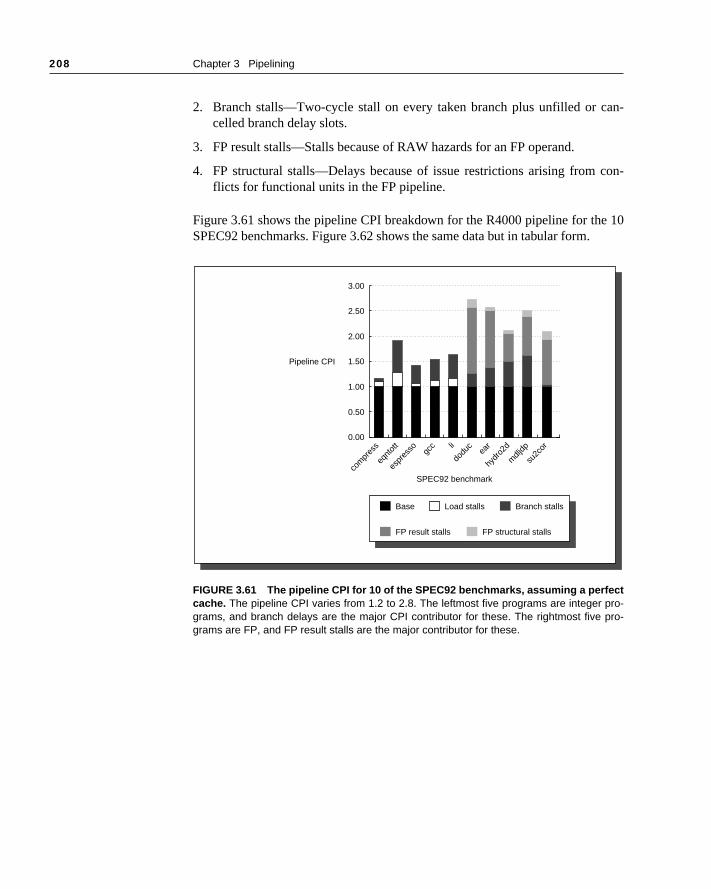
208 Chapter 3 Pipelining
an-
con-
e 10
2. Branch stalls—Two-cycle stall on every taken branch plus unfilled or ccelled branch delay slots.
3. FP result stalls—Stalls because of RAW hazards for an FP operand.
4. FP structural stalls—Delays because of issue restrictions arising from flicts for functional units in the FP pipeline.
Figure 3.61 shows the pipeline CPI breakdown for the R4000 pipeline for thSPEC92 benchmarks. Figure 3.62 shows the same data but in tabular form.
FIGURE 3.61 The pipeline CPI for 10 of the SPEC92 benchmarks, assuming a perfectcache. The pipeline CPI varies from 1.2 to 2.8. The leftmost five programs are integer pro-grams, and branch delays are the major CPI contributor for these. The rightmost five pro-grams are FP, and FP result stalls are the major contributor for these.
Pipeline CPI
0.00
3.00
0.50
1.00
2.00
1.50
2.50
SPEC92 benchmarkco
mpr
ess
eqnt
ott
espr
esso gc
c li
dodu
cea
r
hydr
o2d
mdlj
dp
su2c
or
Load stalls Branch stallsBase
FP structural stallsFP result stalls

3.10 Fallacies and Pitfalls 209
eeperfive-e cy-ranche FP bothtsionsunc-ctur-s.
.
om-ninge firstt the
:
From the data in Figures 3.61 and 3.62, we can see the penalty of the dpipelining. The R4000’s pipeline has much longer branch delays than the stage DLX-style pipeline. The longer branch delay substantially increases thcles spent on branches, especially for the integer programs with a higher bfrequency. An interesting effect for the FP programs is that the latency of thfunctional units leads to more stalls than the structural hazards, which arisefrom the initiation interval limitations and from conflicts for functional unifrom different FP instructions. Thus, reducing the latency of FP operatshould be the first target, rather than more pipelining or replication of the ftional units. Of course, reducing the latency would probably increase the strual stalls, since many potential structural stalls are hidden behind data hazard
Pitfall: Unexpected execution sequences may cause unexpected hazards
At first glance, WAW hazards look like they should never occur because no cpiler would ever generate two writes to the same register without an interveread. But they can occur when the sequence is unexpected. For example, thwrite might be in the delay slot of a taken branch when the scheduler thoughbranch would not be taken. Here is the code sequence that could cause this
Benchmark Pipeline CPI Load stalls Branch stalls FP result stalls FP structural stalls
compress 1.20 0.14 0.06 0.00 0.00
eqntott 1.88 0.27 0.61 0.00 0.00
espresso 1.42 0.07 0.35 0.00 0.00
gcc 1.56 0.13 0.43 0.00 0.00
li 1.64 0.18 0.46 0.00 0.00
Integer average 1.54 0.16 0.38 0.00 0.00
doduc 2.84 0.01 0.22 1.39 0.22
mdljdp2 2.66 0.01 0.31 1.20 0.15
ear 2.17 0.00 0.46 0.59 0.12
hydro2d 2.53 0.00 0.62 0.75 0.17
su2cor 2.18 0.02 0.07 0.84 0.26
FP average 2.48 0.01 0.33 0.95 0.18
Overall average 2.00 0.10 0.36 0.46 0.09
FIGURE 3.62 The total pipeline CPI and the contributions of the four major sources of stalls are shown. The majorcontributors are FP result stalls (both for branches and for FP inputs) and branch stalls, with loads and FP structural stallsadding less.
3.10 Fallacies and Pitfalls

210 Chapter 3 Pipelining
ue ofine. andndler.
g to
f the cy- a 55-tes at 45
, butes the
rfor-
ing.er ofue tombine.63
ce forum-
tion isms,
ning
ode.
s that op-yed
BNEZ R1,foo
DIVD F0,F2,F4 ; moved into delay slot
; from fall through
.....
.....
foo: LD F0,qrs
If the branch is taken, then before the DIVD can complete, the LD will reach WB,causing a WAW hazard. The hardware must detect this and may stall the issthe LD. Another way this can happen is if the second write is in a trap routThis occurs when an instruction that traps and is writing results continuescompletes after an instruction that writes the same register in the trap haThe hardware must detect and prevent this as well.
Pitfall: Extensive pipelining can impact other aspects of a design, leadinoverall worse cost/performance.
The best example of this phenomenon comes from two implementations oVAX, the 8600 and the 8700. When the 8600 was initially delivered, it had acle time of 80 ns. Subsequently, a redesigned version, called the 8650, withns clock was introduced. The 8700 has a much simpler pipeline that operathe microinstruction level, yielding a smaller CPU with a faster clock cycle ofns. The overall outcome is that the 8650 has a CPI advantage of about 20%the 8700 has a clock rate that is about 20% faster. Thus, the 8700 achievsame performance with much less hardware.
Fallacy: Increasing the number of pipeline stages always increases pemance.
Two factors combine to limit the performance improvement gained by pipelinLimited parallelism in the instruction stream means that increasing the numbpipeline stages, called the pipeline depth, will eventually increase the CPI, ddependences that require stalls. Second, clock skew and latch overhead coto limit the decrease in clock period obtained by further pipelining. Figure 3shows the trade-off between the number of pipeline stages and performanthe first 14 of the Livermore Loops. The performance flattens out when the nber of pipeline stages reaches 4 and actually drops when the execution porpipelined 16 deep. Although this study is limited to a small set of FP prograthe trade-off of increasing CPI versus increasing clock rate by more pipeliarises constantly.
Pitfall: Evaluating a compile-time scheduler on the basis of unoptimized c
Unoptimized code—containing redundant loads, stores, and other operationmight be eliminated by an optimizer—is much easier to schedule than “tight”timized code. This holds for scheduling both control delays (with dela

3.11 Concluding Remarks 211
000,ock opti-aster, opti-ther
tech-e via950sion ofrove-inte-e in setsoff.
uctione re- that will
branches) and delays arising from RAW hazards. In gcc running on an R3which has a pipeline almost identical to that of DLX, the frequency of idle clcycles increases by 18% from the unoptimized and scheduled code to themized and scheduled code. Of course, the optimized program is much fsince it has fewer instructions. To fairly evaluate a scheduler you must usemized code, since in the real system you will derive good performance from ooptimizations in addition to scheduling.
Pipelining has been and is likely to continue to be one of the most important niques for enhancing the performance of processors. Improving performancpipelining was the key focus of many early computer designers in the late 1through the mid 1960s. In the late 1960s through the late 1970s, the attentcomputer architects was focused on other things, including the dramatic impments in cost, size, and reliability that were achieved by the introduction of grated circuit technology. In this period pipelining played a secondary rolmany designs. Since pipelining was not a primary focus, many instructiondesigned in this period made pipelining overly difficult and reduced its payThe VAX architecture is perhaps the best example.
In the late 1970s and early 1980s several researchers realized that instrset complexity and implementation ease, particularly ease of pipelining, werlated. The RISC movement led to a dramatic simplification in instruction setsallowed rapid progress in the development of pipelining techniques. As we
FIGURE 3.63 The depth of pipelining versus the speedup obtained. The x-axis showsthe number of stages in the EX portion of the floating-point pipeline. A single-stage pipelinecorresponds to 32 levels of logic, which might be appropriate for a single FP operation. Databased on Table 2 in Kunkel and Smith [1986].
3.11 Concluding Remarks
1 2 4 8 16
Pipeline depth
3.0
2.5
1.5Relativeperformance
1.0
0.5
0.0
2.0

212 Chapter 3 Pipelining
icated.ould
0s. omepro-e rep-. Tontro-ch pre-e ofe the
with
, theast-me—pingand use
ucedt de-
s andasic
Ra- en- theyclese a
tionarly
in in-IPS
r theenta-rs of
see in the next chapter, these techniques have become extremely sophistThe sophisticated implementation techniques now in use in many designs whave been extremely difficult with the more complex architectures of the 197
In this chapter, we introduced the basic ideas in pipelining and looked at ssimple compiler strategies for enhancing performance. The pipelined microcessors of the 1980s relied on these strategies, with the R4000-style machinresenting one of the most advanced of the “simple” pipeline organizationsfurther improve performance in this decade most microprocessors have iduced schemes such as hardware-based pipeline scheduling, dynamic brandiction, the ability to issue more than one instruction in a cycle, and the usmore powerful compiler technology. These more advanced techniques arsubject of the next chapter.
This section describes some of the major advances in pipelining and endssome of the recent literature on high-performance pipelining.
The first general-purpose pipelined machine is considered to be StretchIBM 7030. Stretch followed the IBM 704 and had a goal of being 100 times fer than the 704. The goal was a stretch from the state of the art at that tihence the nickname. The plan was to obtain a factor of 1.6 from overlapfetch, decode, and execute, using a four-stage pipeline. Bloch [1959] Bucholtz [1962] describe the design and engineering trade-offs, including theof ALU bypasses. The CDC 6600, developed in the early 1960s, also introdseveral enhancements in pipelining; these innovations and the history of thasign are discussed in the next chapter.
A series of general pipelining descriptions that appeared in the late 1970early 1980s provided most of the terminology and described most of the btechniques used in simple pipelines. These surveys include Keller [1975],mamoorthy and Li [1977], Chen [1980], and Kogge’s book [1981], devotedtirely to pipelining. Davidson and his colleagues [1971, 1975] developedconcept of pipeline reservation tables as a design methodology for multicpipelines with feedback (also described in Kogge [1981]). Many designers uvariation of these concepts, as we did in sections 3.2 and 3.3.
The RISC machines were originally designed with ease of implementaand pipelining in mind. Several of the early RISC papers, published in the e1980s, attempt to quantify the performance advantages of the simplification struction set. The best analysis, however, is a comparison of a VAX and a Mimplementation published by Bhandarkar and Clark in 1991, 10 years aftefirst published RISC papers. After 10 years of arguments about the implemtion benefits of RISC, this paper convinced even the most skeptical designethe advantages of a RISC instruction set architecture.
3.12 Historical Perspective and References

3.12 Historical Perspective and References 213
the nextin mi-fordpilerulingen-
andpter.ouldctiontatic
essy
g in-r ma- andellent988] and
tion-
ro-991]imi- in
C
The RISC machines refined the notion of compiler-scheduled pipelines inearly 1980s, though earlier work on this topic is described at the end of thechapter. The concepts of delayed branches and delayed loads—common croprogramming—were extended into the high-level architecture. The StanMIPS architecture made the pipeline structure purposely visible to the comand allowed multiple operations per instruction. Simple schemes for schedthe pipeline in the compiler were described by Sites [1979] for the Cray, by Hnessy and Gross [1983] (and in Gross’s thesis [1983]), and by GibbonsMuchnik [1986]. More advanced techniques will be described in the next chaRymarczyk [1982] describes the interlock conditions that programmers shbe aware of for a 360-like machine; this paper also shows the complex interabetween pipelining and an instruction set not designed to be pipelined. Sbranch prediction by profiling has been explored by McFarling and Henn[1986] and by Fisher and Freudenberger [1992].
J. E. Smith and his colleagues have written a number of papers examininstruction issue, exception handling, and pipeline depth for high-speed scalachines. Kunkel and Smith [1986] evaluate the impact of pipeline overheaddependences on the choice of optimal pipeline depth; they also have an excdiscussion of latch design and its impact on pipelining. Smith and Pleszkun [1evaluate a variety of techniques for preserving precise exceptions. WeissSmith [1984] evaluate a variety of hardware pipeline scheduling and instrucissue techniques.
The MIPS R4000, in addition to being one of the first deeply pipelined micprocessors, was the first true 64-bit architecture. It is described by Killian [1and by Heinrich [1993]. The initial Alpha implementation (the 21064) has a slar instruction set and similar integer pipeline structure, with more pipeliningthe floating-point unit.
References
BHANDARKAR, D. AND D. W. CLARK [1991]. “Performance from architecture: Comparing a RISand a CISC with similar hardware organizations,” Proc. Fourth Conf. on Architectural Support forProgramming Languages and Operating Systems, IEEE/ACM (April), Palo Alto, Calif., 310–319.
BLOCH, E. [1959]. “The engineering design of the Stretch computer,” Proc. Fall Joint ComputerConf., 48–59.
BUCHOLTZ, W. [1962]. Planning a Computer System: Project Stretch, McGraw-Hill, New York.
CHEN, T. C. [1980]. “Overlap and parallel processing,” in Introduction to Computer Architecture, H.Stone, ed., Science Research Associates, Chicago, 427–486.
CLARK, D. W. [1987]. “Pipelining and performance in the VAX 8800 processor,” Proc. Second Conf.on Architectural Support for Programming Languages and Operating Systems, IEEE/ACM(March), Palo Alto, Calif., 173–177.
DAVIDSON, E. S. [1971]. “The design and control of pipelined function generators,” Proc. Conf. onSystems, Networks, and Computers, IEEE (January), Oaxtepec, Mexico, 19–21.
DAVIDSON, E. S., A. T. THOMAS, L. E. SHAR, AND J. H. PATEL [1975]. “Effective control for pipe-lined processors,” COMPCON, IEEE (March), San Francisco, 181–184.
EARLE, J. G. [1965]. “Latched carry-save adder,” IBM Technical Disclosure Bull. 7 (March), 909–910.

214 Chapter 3 Pipelining
1/
snd
-
-
,”
EMER, J. S. AND D. W. CLARK [1984]. “A characterization of processor performance in the VAX-1780,” Proc. 11th Symposium on Computer Architecture (June), Ann Arbor, Mich., 301–310.
FISHER, J. AND FREUDENBERGER, S. [1992]. “Predicting conditional branch directions from previouruns of a program,” Proc. Fifth Conf. on Architectural Support for Programming Languages aOperating Systems, IEEE/ACM (October), Boston, 85–95.
GIBBONS, P. B. AND S. S. MUCHNIK [1986]. “Efficient instruction scheduling for a pipelined processor,” SIGPLAN ‘86 Symposium on Compiler Construction, ACM (June), Palo Alto, Calif., 11–16.
GROSS, T. R. [1983]. Code Optimization of Pipeline Constraints, Ph.D. Thesis (December), Computer Systems Lab., Stanford Univ.
HEINRICH, J. [1993]. MIPS R4000 User’s Manual, Prentice Hall, Englewood Cliffs, N.J.
HENNESSY, J. L. AND T. R. GROSS [1983]. “Postpass code optimization of pipeline constraints,” ACMTrans. on Programming Languages and Systems 5:3 (July), 422–448.
IBM [1990]. “The IBM RISC System/6000 processor” (collection of papers), IBM J. of Research andDevelopment 34:1 (January).
KELLER R. M. [1975]. “Look-ahead processors,” ACM Computing Surveys 7:4 (December), 177–195.
KILLIAN , E. [1991]. “MIPS R4000 technical overview–64 bits/100 MHz or bust,” Hot Chips III Sym-posium Record (August), Stanford University, 1.6–1.19.
KOGGE, P. M. [1981]. The Architecture of Pipelined Computers, McGraw-Hill, New York.
KUNKEL, S. R. AND J. E. SMITH [1986]. “Optimal pipelining in supercomputers,” Proc. 13th Sym-posium on Computer Architecture (June), Tokyo, 404–414.
MCFARLING, S. AND J. L. HENNESSY [1986]. “Reducing the cost of branches,” Proc. 13th Symposiumon Computer Architecture (June), Tokyo, 396-403.
RAMAMOORTHY, C. V. AND H. F. LI [1977]. “Pipeline architecture,” ACM Computing Surveys 9:1(March), 61–102.
RYMARCZYK , J. [1982]. “Coding guidelines for pipelined processors,” Proc. Symposium on Archi-tectural Support for Programming Languages and Operating Systems, IEEE/ACM (March), PaloAlto, Calif., 12–19.
SITES, R. [1979]. Instruction Ordering for the CRAY-1 Computer, Tech. Rep. 78-CS-023 (July),Dept. of Computer Science, Univ. of Calif., San Diego.
SMITH, J. E. AND A. R. PLESZKUN [1988]. “Implementing precise interrupts in pipelined processorsIEEE Trans. on Computers 37:5 (May), 562–573.
WEISS, S. AND J. E. SMITH [1984]. “Instruction issue logic for pipelined supercomputers,” Proc. 11thSymposium on Computer Architecture (June), Ann Arbor, Mich., 110–118.
E X E R C I S E S
3.1 [15/15/15] <3.4,3.5> Use the following code fragment:
loop: LW R1,0(R2)
ADDI R1,R1,#1
SW 0(R2),R1
ADDI R2,R2,#4
SUB R4,R3,R2
BNEZ R4,Loop

Exercises 215
es are
line writese ad bydoes
ithureIf allcute?
andp in-uale the
ow ae en-
) andzardser in-
ipe-nd a
.10. han-any
Assume that the initial value of R3 is R2 + 396.
Throughout this exercise use the DLX integer pipeline and assume all memory accesscache hits.
a. [15] <3.4,3.5> Show the timing of this instruction sequence for the DLX pipewithout any forwarding or bypassing hardware but assuming a register read and ain the same clock cycle “forwards” through the register file, as in Figure 3.10. Upipeline timing chart like Figure 3.14 or 3.15. Assume that the branch is handleflushing the pipeline. If all memory references hit in the cache, how many cycles this loop take to execute?
b. [15] <3.4,3.5> Show the timing of this instruction sequence for the DLX pipeline wnormal forwarding and bypassing hardware. Use a pipeline timing chart like Fig3.14 or 3.15. Assume that the branch is handled by predicting it as not taken. memory references hit in the cache, how many cycles does this loop take to exe
c. [15] <3.4,3.5> Assuming the DLX pipeline with a single-cycle delayed branch normal forwarding and bypassing hardware, schedule the instructions in the loocluding the branch-delay slot. You may reorder instructions and modify the individinstruction operands, but do not undertake other loop transformations that changnumber or opcode of the instructions in the loop (that’s for the next chapter!). Shpipeline timing diagram and compute the number of cycles needed to execute thtire loop.
3.2 [15/15/15] <3.4,3.5,3.7> Use the following code fragment:
Loop: LD F0,0(R2)
LD F4,0(R3)
MULTD F0,F0,F4
ADDD F2,F0,F2
ADDI R2,R2,#8
ADDI R3,R3,#8
SUB R5,R4,R2
BNEZ R5,Loop
Assume that the initial value of R4 is R2 + 792.
For this exercise assume the standard DLX integer pipeline (as shown in Figure 3.10the standard DLX FP pipeline as described in Figures 3.43 and 3.44. If structural haare due to write-back contention, assume the earliest instruction gets priority and othstructions are stalled.
a. [15] <3.4,3.5,3.7> Show the timing of this instruction sequence for the DLX FP pline without any forwarding or bypassing hardware but assuming a register read awrite in the same clock cycle “forwards” through the register file, as in Figure 3Use a pipeline timing chart like Figure 3.14 or 3.15. Assume that the branch isdled by flushing the pipeline. If all memory references hit in the cache, how mcycles does this loop take to execute?

216 Chapter 3 Pipelining
ipe-likeen. Ife to
nchp in-uale the
ow aentire
for aister- mode
achineline
andis both
rite of
enter;need
b. [15] <3.4,3.5,3.7> Show the timing of this instruction sequence for the DLX FP pline with normal forwarding and bypassing hardware. Use a pipeline timing chart Figure 3.14 or 3.15. Assume that the branch is handled by predicting it as not takall memory references hit in the cache, how many cycles does this loop takexecute?
c. [15] <3.4,3.5,3.7> Assuming the DLX FP pipeline with a single-cycle delayed braand full bypassing and forwarding hardware, schedule the instructions in the loocluding the branch-delay slot. You may reorder instructions and modify the individinstruction operands, but do not undertake other loop transformations that changnumber or opcode of the instructions in the loop (that’s for the next chapter!). Shpipeline timing diagram and compute the time needed in cycles to execute the loop.
3.3 [12/13/20/20/15/15] <3.2,3.4,3.5> For these problems, we will explore a pipeline register-memory architecture. The architecture has two instruction formats: a regregister format and a register-memory format. There is a single-memory addressing(offset + base register).
There is a set of ALU operations with format:
ALUop Rdest, Rsrc 1, Rsrc 2
or
ALUop Rdest, Rsrc 1, MEM
where the ALUop is one of the following: Add, Subtract, And, Or, Load (Rsrc1 ignored),Store. Rsrc or Rdest are registers. MEM is a base register and offset pair.
Branches use a full compare of two registers and are PC-relative. Assume that this mis pipelined so that a new instruction is started every clock cycle. The following pipestructure—similar to that used in the VAX 8700 micropipeline (Clark [1987])—is
The first ALU stage is used for effective address calculation for memory referencesbranches. The second ALU cycle is used for operations and branch comparison. RF a decode and register-fetch cycle. Assume that when a register read and a register wthe same register occur in the same clock the write data is forwarded.
a. [12] <3.2> Find the number of adders needed, counting any adder or incremshow a combination of instructions and pipe stages that justify this answer. You only give one combination that maximizes the adder count.
IF RF ALU1 MEM ALU2 WB
IF RF ALU1 MEM ALU2 WB
IF RF ALU1 MEM ALU2 WB
IF RF ALU1 MEM ALU2 WB
IF RF ALU1 MEM ALU2 WB
IF RF ALU1 MEM ALU2 WB

Exercises 217
writetruc- and
dinge twot ig-ning
stallsat asfrom
an anting
stall.
pipe-ed andus the to 20 worklot the
ngat thehen-ver-f any
(for
ipe- we
b. [13] <3.2> Find the number of register read and write ports and memory read andports required. Show that your answer is correct by showing a combination of instions and pipeline stage indicating the instruction and the number of read portswrite ports required for that instruction.
c. [20] <3.4> Determine any data forwarding for any ALUs that will be needed. Assumethat there are separate ALUs for the ALU1 and ALU2 pipe stages. Put in all forwaramong ALUs needed to avoid or reduce stalls. Show the relationship between thinstructions involved in forwarding using the format of the table in Figure 3.19 bunoring the last two columns. Be careful to consider forwarding across an interveinstruction, e.g.,
ADD R1, ...
any instruction
ADD ..., R1, ...
d. [20] <3.4> Show all data forwarding requirements needed to avoid or reduce when either the source or destination unit is not an ALU. Use the same formFigure 3.19, again ignoring the last two columns. Remember to forward to and memory references.
e. [15] <3.4> Show all the remaining hazards that involve at least one unit other thALU as the source or destination unit. Use a table like that in Figure 3.18, but listhe length of hazard in place of the last column.
f. [15] <3.5> Show all control hazard types by example and state the length of theUse a format like Figure 3.21, labeling each example.
3.4 [10] <3.2> Consider the example on page 137 that compares the unpipelined andlined machine. Assume that 1 ns overhead is fixed and that each pipe stage is balanctakes 10 ns in the five-stage pipeline. Plot the speedup of the pipelined machine versunpipelined machine as the number of pipeline stages is increased from five stagesstages, considering only the impact of the pipelining overhead and assuming that thecan be evenly divided as the stages are increased (which is not generally true). Also p“perfect” speedup that would be obtained if there was no overhead.
3.5 [12] <3.1–3.5> A machine is called “underpipelined” if additional levels of pipelinican be added without changing the pipeline-stall behavior appreciably. Suppose thDLX integer pipeline was changed to four stages by merging EX and MEM and lengting the clock cycle by 50%. How much faster would the conventional DLX pipeline be sus the underpipelined DLX on integer code only? Make sure you include the effect ochange in pipeline stalls using the data for gcc in Figure 3.38 (page 178).
3.6 [20] <3.4> Add the forwarding entries for stores and for the zero detect unit branches) to the table in Figure 3.19. Hint: Remember the tricky case:
ADD R1, ...
any instruction
SW ..., R1
How is the forwarding handled for this case?
3.7 [20] <3.4,3.9> Create a table showing the forwarding logic for the R4000 integer pline using the same format as that in Figure 3.19. Include only the DLX instructionsconsidered in Figure 3.19.

218 Chapter 3 Pipelining
g theat we
are as
e sec-onalwheth-chine
resultth of
tage
basic
zard
ardse 1 ofot. Weyieldhes in
3.8 [15] <3.4,3.9> Create a table showing the R4000 integer hazard detection usinsame format as that in Figure 3.18. Include only the instructions in the DLX subset thconsidered in section 3.4.
3.9 [15] <3.5> Suppose the branch frequencies (as percentages of all instructions) follows:
Conditional branches 20%Jumps and calls 5%Conditional branches 60% are taken
We are examining a four-deep pipeline where the branch is resolved at the end of thond cycle for unconditional branches and at the end of the third cycle for conditibranches. Assuming that only the first pipe stage can always be done independent of er the branch goes and ignoring other pipeline stalls, how much faster would the mabe without any branch hazards?
3.10 [20/20] <3.4> Suppose that we have the pipeline layout shown in Figure 3.64.
All data dependences are between the register written in stage 3 of instruction i and a reg-ister read in stage 2 of instruction i + 1, before instruction i has completed. The probabilityof such an interlock occurring is 1/p.
We are considering a change in the machine organization that would write back the of an instruction during an effective fourth pipe stage. This would decrease the lengthe clock cycle by d (i.e., if the length of the clock cycle was T, it is now T – d). The prob-ability of a dependence between instruction i and instruction i + 2 is p–2. (Assume that thevalue of p–1 excludes instructions that would interlock on i + 2.) The branch would also beresolved during the fourth stage.
a. [20] <3.4> Assume that we add no additional forwarding hardware for the four-spipeline. Considering only the data hazard, find the lower bound on d that makes thisa profitable change. Assume that each result has exactly one use and that theclock cycle has length T.
b. [20] <3.4> Now assume that we have used forwarding to eliminate the extra haintroduced by the change. That is, for all data hazards the pipeline length is effectively3. This design may still not be worthwhile because of the impact of control hazcoming from a four-stage versus a three-stage pipeline. Assume that only stagthe pipeline can be safely executed before we decide whether a branch goes or nwant to know the impact of branch hazards before this longer pipeline does not high performance. Find an upper bound on the percentages of conditional branc
Stage Function
1 Instruction fetch
2 Operand decode
3 Execution or memory access (branch resolution)
FIGURE 3.64 Pipeline stages.

Exercises 219
rr-e the
lls forinter-
.44ds to
tablepipe-
LX
s for
thency off for-and
m-d FPst sus-
blylator.
with
programs in terms of the ratio of d to the original clock-cycle time, so that the longepipeline has better performance. If d is a 10% reduction, what is the maximum pecentage of conditional branches before we lose with this longer pipeline? Assumtaken-branch frequency for conditional branches is 60%.
3.11 [20] <3.4,3.7> Construct a table like Figure 3.18 that shows the data hazard stathe DLX FP pipeline as shown in Figure 3.44. Consider both integer-FP and FP-FP actions but ignore divides (FP and integer).
3.12 [20] <3.4,3.7> Construct the forwarding table for the DLX FP pipeline of Figure 3as we did in Figure 3.19. Consider both FP to FP forwarding and forwarding of FP loathe FP units but ignore FP and integer divides.
3.13 [25] <3.4,3.7> Suppose DLX had only one register set. Construct the forwarding for the FP and integer instructions using the format of Figure 3.19. Assume the DLX line in Figure 3.44. Ignore FP and integer divides.
3.14 [15] <3.4,3.7> Construct a table like Figure 3.18 to check for WAW stalls in the DFP pipeline of Figure 3.44. Do not consider integer or FP divides.
3.15 [20] <3.4,3.7> Construct a table like Figure 3.18 that shows the structural stallthe R4000 FP pipeline.
3.16 [35] <3.2–3.7> Change the DLX instruction simulator to be pipelined. Measurefrequency of empty branch-delay slots, the frequency of load delays, and the frequeFP stalls for a variety of integer and FP programs. Also, measure the frequency owarding operations. Determine the performance impact of eliminating forwarding stalling.
3.17 [35] <3.7> Using a DLX simulator, create a DLX pipeline simulator. Explore the ipact of lengthening the FP pipelines, assuming both fully pipelined and unpipelineunits. How does clustering of FP operations affect the results? Which FP units are moceptible to changes in the FP pipeline length?
3.18 [40] <3.3–3.5> Write an instruction scheduler for DLX that works on DLX assemlanguage. Evaluate your scheduler using either profiles of programs or a pipeline simuIf the DLX C compiler does optimization, evaluate your scheduler’s performance both and without optimization.