pism, a parallel ice sheet model: user’s …it documents all the pism options. it describes how to...
TRANSCRIPT

PISM, A PARALLEL ICE SHEET MODEL:
USER’S MANUAL
ED BUELER
CONSTANTINE KHROULEV
JED BROWN
NATHAN SHEMONSKI
Date: March 31, 2009. Support by email: [email protected]. Based on PISM revision 645
(stable0.2) and PETSC release 2.3.3 or 3.0.0. Get stable version of PISM source code:
svn co http://svn.gna.org/svn/pism/tags/stable0.2 pism0.2 .

2 PISM USER’S MANUAL
Copyright (C) 2004–2009 Ed Bueler and Constantine Khroulev and Jed
Brown and Nathan Shemonski
This file is part of PISM.
PISM is free software; you can redistribute it and/or modify it under
the terms of the GNU General Public License as published by the Free
Software Foundation; either version 2 of the License, or (at your option)
any later version. PISM is distributed in the hope that it will be useful,
but WITHOUT ANY WARRANTY; without even the implied warranty of
MERCHANTABILITY or FITNESS FOR A PARTICULAR PURPOSE.
See the GNU General Public License for more details. You should have
received a copy of the GNU General Public License along with PISM; see
COPYING. If not, write to the Free Software Foundation, Inc., 51 Franklin
St, Fifth Floor, Boston, MA 02110-1301 USA
Acknowledgements
The NASA Modeling, Analysis, and Prediction program, funded proposal 08-MAP-0108, supports the development of PISM. Development from 2003 to 2008 was supportedby the NASA Cryospheric Sciences Program, grant NAG5-11371.
The Arctic Regional Supercomputer Center has provided significant computational re-sources and technical help in the development of PISM.
Our research into ice sheet modeling was strongly influenced and constantly motivatedby Craig Lingle. Dave Covey, Don Bahls, and Greg Newby have supported our comput-ers, tools, and and computations. Thanks to Tolly Adalgeirsdottir, Andy Aschwanden,Torsten Albrecht, Marianne Hasselhoff, Tore Hattermann, Jesse Johnson, Art Mahoney,Anders Levermann, Maria Martin, Kent Overstreet, Martin Truffer, Ben Sperisen, Ri-carda Winkelmann, Ryan Woodard and several other PISM users for helpful commentsand questions on PISM and this Manual.

PISM USER’S MANUAL 3
Contents
1. Introduction 42. Getting started 52.1. Running an EISMINT simplified geometry experiment 52.2. PISM’s standard output 82.3. Handling NetCDF files 93. Ice dynamics, the PISM view 103.1. Principles 103.2. Two main shallow models, SIA and SSA 103.3. A hierarchy of simplifying assumptions for ice flow 113.4. Evolutionary versus diagnostic ice shelf modeling 113.5. Separation of climate inputs from ice dynamics 124. Initialization and bootstrapping 155. Usage 185.1. Computational box 185.2. Grid 185.3. Regridding 195.4. Adaptive time-stepping 215.5. Signals, to control a running PISM model 215.6. Saving snapshots of the model state 235.7. Positive degree-day model 245.8. Floatation criterion and mask 255.9. Earth deformation models 265.10. Diagnostic computations 265.11. Plastic till free boundary problem for ice streams; SSA as a sliding law 275.12. Visualizing the climate inputs, without ice dynamics 286. Verification 307. Simplified geometry experiments 367.1. Historical note 367.2. EISMINT II in PISM 367.3. MISMIP in PISM 388. Example: Modeling the Greenland ice sheet 459. Example: Validating PISM as a flow model for the Ross ice shelf 58References 64Appendix A. PISM command line options 67A.1. List of PISM options 67A.2. PETSC options for PISM users 78Appendix B. PISM viewers: Graphical and Matlab 80Appendix C. Python scripts for PISM modeling 83Index 87
4 PISM USER’S MANUAL
1. Introduction
Welcome! All information about PISM is online atwww.pism-docs.org
See the Installation Manual for how to download the PISM source code and install it andthe libraries it needs.
This User’s Manual and the Installation Manual can be generated from any copy ofthe PISM source code by doing make userman installation in the PISM root directoryand then viewing doc/manual.pdf and doc/installation.pdf with a PDF viewer.
This User’s Manual describes how to run PISM for certain simplified geometry situa-tions and it illustrates how PISM’s numerical approximations are verified. It documentsall the PISM options. It describes how to use PISM as a Greenland ice sheet model or aRoss ice shelf model, based on certain publicly-available data.
Users who want to advance the science of ice sheets will need to go beyond what isdescribed here. For such users there are two additional documents to know about:
(1) The C++ Class Browser gives a complete view of the class/object structure ofthe source code. It is the best tool for understanding the internals of PISM, andfor the job of modifying and supplementing PISM by writing derived classes. It isonline at
www.pism-docs.org/doxy/html/index.html
The Browser can be generated from the source by doing make browser in thePISM root directory and then viewing doc/doxy/html/index.html.
(2) The Reference Manual documents only the continuum models and numericalmethods of PISM. A current Reference Manual can be generated from the sourceby doing make refman in the PISM root directory and then viewing doc/refman.pdf.
The C++ Class Browser and the Reference Manual are automatically generated bydoxygen (www.doxygen.org) from comments in the PISM source code.
WARNING : PISM is an ongoing project. Ice sheet modeling is com-
plicated and is generally not mature. Please don’t trust the results of
PISM or any other ice sheet model without a fair amount of exploration.
Also, please don’t expect all your questions to be answered here. Write
to us with questions.

PISM USER’S MANUAL 5
2. Getting started
See the Installation Manual to install PISM. Once installed, the pgrn, pismd, pismr,pisms, and pismv executables will be in the bin subdirectory of the PISM root directory.The User’s Manual addresses the use of all five executables. This Getting started sectiononly uses pisms.
2.1. Running an EISMINT simplified geometry experiment. PISM’s purpose isthe simulation of actual ice sheets. But actual ice sheet simulations require actual data.Ice sheet and ice shelf data are freely available as part of the EISMINT intercomparisonefforts. Section 8 is a tutorial on the use of PISM as a Greenland ice sheet evolution modeland section 9 is a tutorial on using PISM as a Ross ice shelf diagnostic model. Both usethe EISMINT data sets.
For now, to avoid issues of data formats, flaws and data-handling scripts in a first useof PISM, this section describes how to use PISM for experiment A in the “EISMINT II”simplified-geometry, thermomechanically-coupled ice sheet model intercomparison [51].This experiment models an angularly-symmetric shallow, grounded ice sheet on a flat bedwith moderately cold surface temperatures.
In EISMINT II the prescribed grid has 60 subintervals in each direction, with eachsubinterval of length 25km. Thus the total width of the computational box is 1500 kmin both x and y directions. However, PISM always allows choice of the grid in all threedimensions. A runtime option chooses the number of grid points in each direction, andthe number of points is one greater than the number of subintervals (grid spaces). Thevertical grid is not prescribed in EISMINT II. For a demonstration we choose a 25kmgrid in the horizontal and we use 41 grid points in the vertical with unequal spacing. Thespacing is finest at the bottom of the ice column (34 m) and coarsest at the top (216 m).The computational box is 5000 m high by default for EISMINT II experiment A in PISM,so no runtime option is needed to set that.
Experiment A starts with zero ice, all EISMINT II runs are for 200,000 model years.The center thickness of the ice sheet grows to a peak near 4100 m, at about 9,000 modelyears, before decaying to its equilibrium center thickness of about 3750 m. Here we startwith a short 6000 year run for a quick illustration. The executable is “pisms”, for the“simplifed geometry mode” of PISM:
$ pisms -eisII A -Mx 61 -My 61 -Mz 41 -quadZ -y 6000
PISMS stable0.2 (simplified geometry mode)
setting parameters for EISMINT II experiment A ...
initializing EISMINT II experiment A ...
[computational box for ice: 1500.00 km x 1500.00 km x 5000.00 m]
[hor. grid cell dimensions: 25.00 km x 25.00 km
vertical grid spacing in ice not equal; range 33.594 m < dz < 216.406 m]
running EISMINT II experiment A ...
P YEAR: ivol iarea meltf thick0 temp0
U years 10^6_km^3 10^6_km^2 (none) m K
S 0.00000: 0.00000 0.0000 0.0000 0.000 273.1500
$$ SIA vath 0m +60.00000
6 PISM USER’S MANUAL
S 60.00000: 0.01704 0.6281 0.0000 30.000 238.1500
. . .
$$ SIA vath 0e +2.05570
S 6000.00000: 1.68054 0.7506 0.0100 3000.000 248.6280
done with run ...
Writing model state to file ‘simp_exper.nc’
This should take less than one minute.In a moment we will address the standard output information provided by PISM,
as shown above, but for now we simply illustrate how to continue and complete the200,000 year run. The model state was stored in a NetCDF file with the (default) namesimp_exper.nc. The next run will use a “-o” option to name the output file. Theabove was a single processor run, but let’s suppose we have a four processor (e.g. fourcores on a single processor, or other arrangement) machine. It should also work fine on asingle processor machine but there is no speed-up, naturally. Let’s also run things in thebackground so we can continue to experiment:
$ mpiexec -n 4 pisms -eisII A -i simp_exper.nc -skip 5 -y 194000 \
-o eisIIA200k.nc >> out.eisIIA &
You can also use -ye 200000 instead of -y 194000 — if you don’t know how long thefirst run was, for example. This run will take less than one wall clock hour, and perhapsmuch less. PISM being parallel, it can be sped up by using more processes. The standardoutput in out.eisIIA can be tracked as the job is running in the background using less,for instance. Also, top is a Linux tool to watch CPU and memory usage during the run.
The run generates a NetCDF file eisIIA200k.nc at the end. The final results forice volume, area, melt fraction, center thickness, and center basal temperature (2.29575106km3, 1.0356 106km2, 0.6156, 3743.075 m, 257.2799 K, respectively) are typical ofEISMINT II intercomparison results shown in Table 4 of [51]. The correctness of PISM’sapproximations of the equations for ice flow is mostly addressed by measuring its errorsrelative to exact solutions to those equations, and not through comparison to averagebehavior of other ice flow models. See section 6 on verification.
To get the model state in the midst of a PISM run, send all running pisms processes(the PISM executable used here) a signal which causes PISM to write out the model state:pkill -USR1 pisms. The PISM model state is then saved in a NetCDF file with namepism-year.nc, using the year at that time step. On the other hand, terminating the runwith pkill -TERM pisms will cause PISM to stop, but only after saving the model stateusing the specified output name. See subsection 5.5 for a more complete description ofhow PISM catches signals.
While the complete run continues in the background, let’s view the intermediate resultstored in simp_exper.nc. An important fact to know is that a PISM output NetCDF filecontains a “history” with the command that produced it. For instance,
$ ncdump -h simp_exper.ncshows the structure (“header”) of the output NetCDF file, with lines like these near thebottom::history = "user@host 2009-02-19 20:28:18 AKST: PISM done. PETSc MFlops = 1.23.\n",

PISM USER’S MANUAL 7
" pisms -eisII A -Mx 61 -My 61 -Mz 41 -quadZ -y 6000\n",
"user@host 2009-02-19 20:27:42 AKST: PISM (...) started on 1 procs.\n",
This kind of “history” is convenient for understanding what you have done, once it allworks!
Figure 1. ncview shows an intermediate stage of an EISMINT II exper-iment A run.
Another way to view the output file is graphically. One of the most convenient toolsis ncview; see Table 1. Running ncview on the output file (ncview simp_exper.nc) andviewing the “thk” variable gives a figure like 1.
Alternatively, one can use PISM’s “diagnostic viewers” for a time-dependent view ofthe evolving modeled ice sheet. Note this requires X Windows:
$ pisms -eisII A -i simp_exper.nc -y 1000 -d HTt
Three figures should appear and be refreshed at each time step. One figure is a map-planeview of thickness, another is a map-plane view of the basal temperature in Kelvin, and thethird is a graph of temperature versus height above the bedrock. When the full 200,000year run finishes, one may watch its evolving, though essentially steady, state. A viewthat includes the ice flow speed is:
$ pisms -eisII A -i eisIIA200k.nc -d HTc
for example. Figure 2 will appear.As shown by the “-d” options above, runtime viewers can be specified by options of the
form -d letters or -dbig letters. The latter option shows larger windows but is otherwiseidentical. See Appendix B for the single letter names of viewers. These viewers areupdated at each time step and are not used for runs in batch mode or where efficiency

8 PISM USER’S MANUAL
Figure 2. Screenshot of diagnostic figures for an EISMINT II experimentA run.
is needed. (As they work under Xwindows, MPI must be told how to send data to thewindow, so PISM options are usually followed by “-display :0” when PISM is run underMPI and runtime viewers are needed.)
2.2. PISM’s standard output. As seen already, at each time step PISM shows a sum-mary of the model state using a few numbers and some single character flags. The formatof the summary is partly explained by two lines near the beginning of the run:
P YEAR: ivol iarea meltf thick0 temp0
U years 10^6_km^3 10^6_km^2 (none) m K
The “P” line is the prototype for the summary which appears at each time step. The“U” line gives units for this summary. From then on, the “S” lines give values for thequantities specified by the “P” and “U” lines.
The EISMINT II runs above illustrate how the time-stepping in PISM adapts in orderto maintain stability for its (mostly) explicit methods. At the beginning of the EISMINTII run, for instance, the ice has small thickness so the time step is 60 years, simply becausethat is the default maximum time step. Later in that run, after about 5000 years, thetime step is made smaller because the flow is faster.
After the year, the next three entries in the summary report the volume of the icein 106 km3, the area covered by the ice in 106 km2, and the basal melt fraction, thatis, the fraction of the ice area where the basal temperature is at the pressure-meltingtemperature. This melted-base-fraction is a pure number without units. The next twocolumns “thick0” and “temp0” are values at the center of the computational domain of
PISM USER’S MANUAL 9
the map plane, namely the ice thickness in meters and the absolute temperature of theice at its base, in Kelvin. These five numbers are the ones reported in the tables in [51],which explains why they are the default quantities for reporting to standard output. Formore on the EISMINT II experiments see section 7.
The summary of the model state can be made more verbose by using the option-verbose.
In addition to the “S” lines, there are lines, starting with a space character, which giveflags, both cryptic and compact, describing the PISM model choices made at each timestep. Most of these relate to decisions of the adaptive time-stepping scheme. That schemeis described in subsection 5.4
If the standard output from PISM is saved in a text file then it can always be convertedto a NetCDF file with corresponding time series. For the 200,000 year run above,
$ series.py -f out.eisIIA -o ser.eisIIA.nc
$ ncview ser.eisIIA.nc
A look at these time series shows the convergence to equilibrium of this non-slidingthermomechanically coupled modeled ice sheet. We see, characteristically, that there isa longer relaxation time for temperature at the base of the ice than for any geometricquantity (volume, area, thickness).
2.3. Handling NetCDF files. At a trivial level, PISM is just a program which takesa NetCDF file as input, does some computation, and produces a NetCDF file as output.(An exception is that pisms knows formulas to initialize EISMINT II experiments, forexample.) The user is in charge of creating NetCDF input files containing data on icesheets worth modeling1, and extracting some meaning from the NetCDF output files.
The most basic tools for converting NetCDF files to and from a standard text repre-sentation are called ncdump and ncgen. A glance at Unix man pages for these tools mightbe wise at this time.
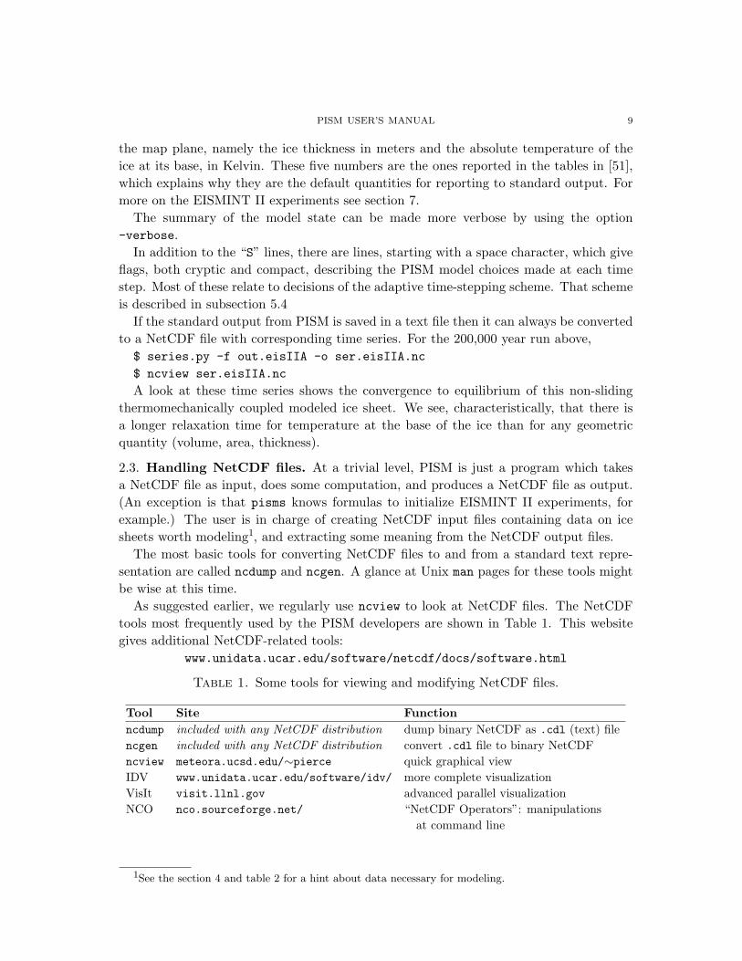
As suggested earlier, we regularly use ncview to look at NetCDF files. The NetCDFtools most frequently used by the PISM developers are shown in Table 1. This websitegives additional NetCDF-related tools:
www.unidata.ucar.edu/software/netcdf/docs/software.html
Table 1. Some tools for viewing and modifying NetCDF files.
Tool Site Functionncdump included with any NetCDF distribution dump binary NetCDF as .cdl (text) filencgen included with any NetCDF distribution convert .cdl file to binary NetCDFncview meteora.ucsd.edu/∼pierce quick graphical viewIDV www.unidata.ucar.edu/software/idv/ more complete visualizationVisIt visit.llnl.gov advanced parallel visualizationNCO nco.sourceforge.net/ “NetCDF Operators”: manipulations
at command line
1See the section 4 and table 2 for a hint about data necessary for modeling.
10 PISM USER’S MANUAL
3. Ice dynamics, the PISM view
3.1. Principles. The main goal of the current section is to give an overview of ice dynam-ics models in PISM, but we list some high-level organizing principles for PISM generally:
(1) source code is open, free, and actually usable with free software tools,(2) science is done with publicly-available data,(3) numerical methods are verifiable by comparison with exact solutions of the mod-
eled equations,(4) models are shallow,(5) the availability of a hierarchy of simplifying ice dynamics assumptions is more
important than any particular set of dynamical equations,(6) everything available diagnostically (instantaneously) is available for evolution,(7) climate inputs affect ice dynamics by a well-defined interface.
We do not claim to follow these principles perfectly. We hope, however, that the user willsee these principles reflected in PISM and this Manual.
Principle (2) is illustrated by sections 8 and 9. Principle (3) is addressed in section 6.Principles (4), (5), (6), and (7) are explained next.
3.2. Two main shallow models, SIA and SSA. PISM can (currently) numericallysolve two significantly different sets of partial differential equations which determine thevelocity field within the ice. In each case the geometry of the ice, the temperature of theice, and the stress condition at the base of the ice are included into balance of momentumequations to determine the flow. But there are two different versions of the balance ofmomentum equations:
• the shallow ice approximation (SIA) [30], which describes ice as flowing by shear inplanes parallel to the geoid, a lubrication approximation [17], with such shearinga local function of the driving stress of classical glaciology [46], and• the shallow shelf approximation (SSA) [68], which describes a membrane-type flow
with the ice floating, or sliding over a weak base [43, 40, 60].
PISM numerically solves both the SIA and SSA equations in parallel. Time-steppingsolutions of the mass continuity equation are possible for both models.
The SIA equations are, as a rule, easier and quicker to numerically solve than the SSA.The SIA equations are also easier to parallelize. They can confidently be applied to thosegrounded parts of ice sheets for which the basal ice is frozen to the bedrock and the bedtopography is relatively slowly-varying in the map-plane [17]. (We recommend solvingthe SIA with a non-sliding base because the ad hoc addition of a “sliding law” whichswitches on at the pressure-melting temperature tends to have unavoidable bad numericalconsequences [9, appendix B]. In PISM the SSA can be used as a sliding law, however.)
The SSA equations can confidently be applied to large floating ice shelves because suchshelves have small depth-to-width ratio and because there is negligible shear stress at thebase of the floating ice [43, 44].
Ice sheets also have fast-flowing grounded parts, however, called “ice streams” or “outletglaciers”. Such features appear at the margin of, and even well into the interior of, the
PISM USER’S MANUAL 11
Greenland [37] and Antarctic [2] ice sheets. Describing these faster-flowing grounded partsof ice sheets requires something more than the non-sliding SIA. Ultimately one might usethe full Stokes equations which represent the balance of all tensor components [17], butthere is still the issue of the appropriate sliding boundary condition. Similarly one mightuse a “higher-order” but still shallow stress balance [5, 48], but again a proper choice ofboundary condition is important.
One may apply the SSA equations with additional basal resistance terms to describefast-flowing grounded ice. This is demonstrated in the context of the Siple Coast icestreams of Antarctica by MacAyeal [40, 28] using a linearly-viscous model for the under-lying till, and in many other referenes. A free boundary problem with essentially the same(SSA) balance equations is the Schoof [60] model of ice streams. In Schoof’s model icestreams emerge in those parts of the ice sheet where there is plastic till failure [46].
As noted, both the SIA and SSA models are shallow approximations. That is, the re-spective partial differential equations are derived by different small-parameter arguments,both based on a small depth-to-width ratio, from the Stokes equations of a non-Newtonianfluid. For this small-parameter argument in the SIA case see [17]. For the correspondingSSA argument, see [68] or the appendices of [60]. See [64] on connections between theseshallowest models and “higher order” models.2
By default, PISM does not numerically solve the SSA. The user must add the option-ssa. (An exception is the use of the executable pismv for verifying the SSA balance ofmomentum equations, as addressed in section 6.)
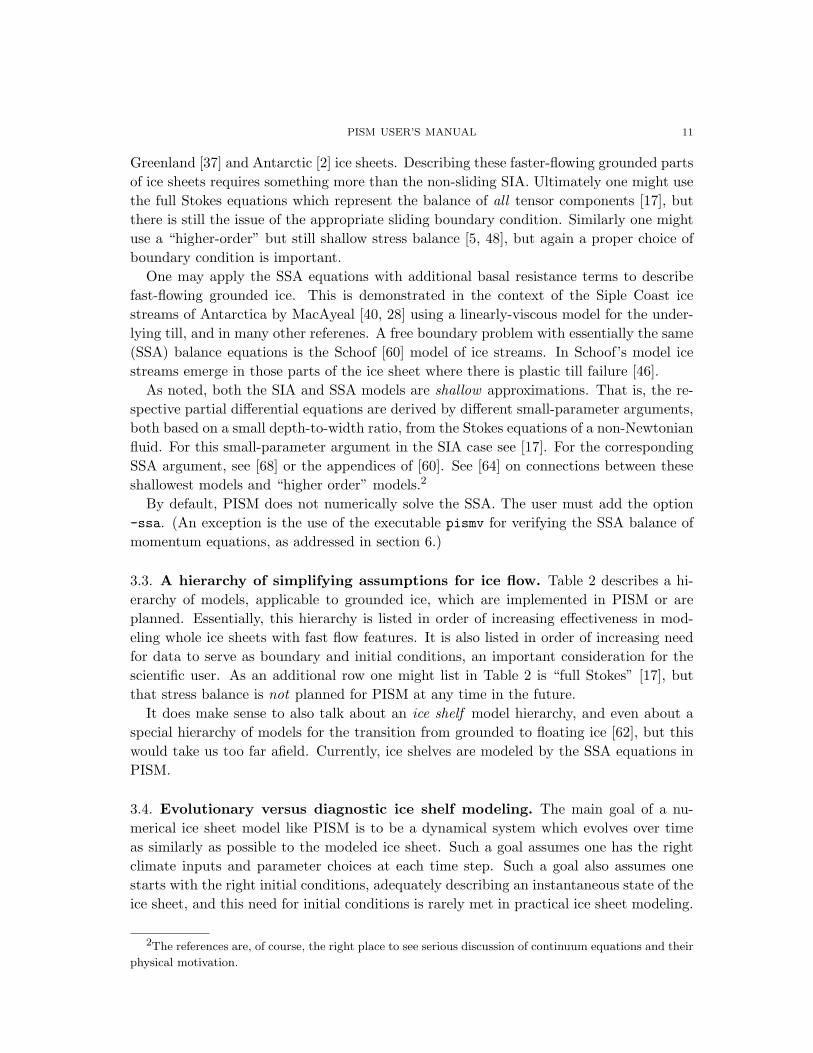
3.3. A hierarchy of simplifying assumptions for ice flow. Table 2 describes a hi-erarchy of models, applicable to grounded ice, which are implemented in PISM or areplanned. Essentially, this hierarchy is listed in order of increasing effectiveness in mod-eling whole ice sheets with fast flow features. It is also listed in order of increasing needfor data to serve as boundary and initial conditions, an important consideration for thescientific user. As an additional row one might list in Table 2 is “full Stokes” [17], butthat stress balance is not planned for PISM at any time in the future.
It does make sense to also talk about an ice shelf model hierarchy, and even about aspecial hierarchy of models for the transition from grounded to floating ice [62], but thiswould take us too far afield. Currently, ice shelves are modeled by the SSA equations inPISM.
3.4. Evolutionary versus diagnostic ice shelf modeling. The main goal of a nu-merical ice sheet model like PISM is to be a dynamical system which evolves over timeas similarly as possible to the modeled ice sheet. Such a goal assumes one has the rightclimate inputs and parameter choices at each time step. Such a goal also assumes onestarts with the right initial conditions, adequately describing an instantaneous state of theice sheet, and this need for initial conditions is rarely met in practical ice sheet modeling.
2The references are, of course, the right place to see serious discussion of continuum equations and their
physical motivation.
12 PISM USER’S MANUAL
Table 2. Hierarchy of current and planned flow models in PISM, for thegrounded parts of ice sheets, from most to fewest simplifying assumptions.(Italicized are planned for future versions of PISM but are not implementedin stable0.2.)
Model Assumptions Needed data Refs.balance velocities steady state, ice flows down surf. mass balance, ice [36]
surface gradient thickness, bed elevationisothermal SIA non-sliding lubrication flow, fixed same, but possibly time- [34, 12]
softness dependentthermomechanically non-sliding lubrication flow, same, plus surf. temperature, [10]
-coupled SIA temperature-dependent softness geothermal fluxSIA + SSA hybrid SSA as a sliding law for thermo- same, plus basal layer (till) [9]
mechanically-coupled SIA strengthBlatter-Pattyn “higher-order”, bridging stresses same [5, 48, 63]
Indeed, underlying an ice sheet model like PISM are evolution-in-time partial differen-tial equations, and PISM generally solves these by taking small time steps3 in approxi-mating these differential equations. We will describe this usual time-stepping behavior asan “evolution run.”
Much modeling, especially of streams and shelves, uses only instantaneous “diagnos-tic” solution of the partial differential equations which determine the velocity field. Theexistence of such “instantaneous” velocity fields follows fromt the slowness of ice, an im-portant simplifying assumption underlying all models in the Table 2 hierarchy. See [17],for example. In a diagnostic computation the temperature field and certain basal condi-tions, such as strength parameters for the till for instance, are held fixed. So the goal ofa “diagnostic run” is to compute the velocity field, including the instantaneous rate ofsurface movement. This will be the definition of that phrase used from now on.
Sections 8 and 9 illustrate the evolutionary versus diagnostic modeling modes. Thefirst is a time-stepping SIA-only model for the Greenland ice sheet while the second is adiagnostic SSA model for the Ross ice shelf.
3.5. Separation of climate inputs from ice dynamics. PISM’s job is to approximateice flow. In addition, as described in subsection 5.9, PISM includes an optional beddeformation component approximating the movement of the Earth’s crust and uppermantle in response to changing ice load. Also, the temperature of a thin layer of bedrockis included in the conservation of energy model for the ice and the till layer.
Thus PISM “handles” the ice and bedrock, when used with other models for the at-mosphere and ocean, as cartooned in Figure 3. “Other models” may be anything fromtrivially-parameterized surface mass balance to full GCMs of astonishing complexity.
3“Small” time steps vary from hundredths to many model years, depending primarily on grid resolution,
but also on modeled ice flow speed.

PISM USER’S MANUAL 13
Figure 3. PISM approximates ice flow and bed deformation, so it“handles” the region below the dashed curve. Components calledPISMAtmosphereCoupler and PISMOceanCoupler provide climate inputsat the ice upper surface and under ice shelves, respectively.
In fact, within the ice dynamics/bed deformation PISM core code, there is no parame-terization or other model for boundary mass or energy balance.4 This is a structural prin-ciple for PISM. Instead, boundary mass or energy balance computations are handled bynon-core interface components called PISMAtmosphereCoupler and PISMOceanCoupler.The former type is for the ice upper surface while the latter type is special to the under-sides of ice shelves. The advantage of this arrangement is that “attaching” PISM to othercomponents of a global or regional climate (circulation) model is intended to be a matteronly of changing a small amount of the PISM interface source code—primarily additionof PISM...Coupler derived classes along with a new driver—without any change to theice dynamics core.
The dashed line in Figure 3 suggests that there is a thin layer on the ice surface notmodeled by PISM. This is true. “Ice dynamics” must include the mass of the snow/firnlayer, but it cannot include the processes which transform this layer into ice with a certaintemperature, below that layer. Similarly, the undersides of ice shelves include (relativelypoorly-understood, but very important!) processes not modeled by core PISM, thoughpotentially modeled in a PISMOceanCoupler. In any case, the job of the PISM...Coupler
components is, as already stated, provide definitive boundary mass or energy balance tothe ice dynamics core.
The PISM source code already contains instances of PISM...Coupler components. Forexample, instances of PISMAtmosphereCoupler exist for the simplified geometry experi-ments in section 7, and for the Greenland model in section 8.
Actually, most of this is invisible to the PISM user. Options given to the PISM exe-cutables (e.g. pismr or pisms) are passed internally to the PISM...Coupler components,so it looks to the user as if command line control of climate inputs is the same as commandline control of ice dynamics. For example, an important kind of PISMAtmosphereCoupler,
4This principle is a change from stable0.1.

14 PISM USER’S MANUAL
namely a positive degree day scheme for surface mass balance, is described in subsection5.7 as a part of PISM. It is part of PISM, but it is outside a well-defined ice dynamicscore.
This structure is important to describe here because, on the one hand, some users maybe interested in coupling PISM to other models. On the other hand, the PISM authorsdo not claim expertise in modeling atmosphere, ocean, or even snow processes, and soseparation has a code-reliability purpose as well. “Users” need to know that they areultimately responsible for providing the climate inputs they intend.
PISM USER’S MANUAL 15
4. Initialization and bootstrapping
“Initialization from a saved model state”. This phrase has a simple meaning in PISM.If a previous PISM run has saved a NetCDF file using “-o” then that file will containcomplete initial conditions for continuing the run. The output file from the last run canbe loaded with “-i”:
$ pisms -eisII A -y 100 -o foo.nc
$ pisms -eisII A -i foo.nc -y 100 -o bar.nc
Note that simplified-geometry experiments (section 7) and verification tests (section 6)do not need input files at all because they initialize from formulas in the source code. Theycan be continued from saved model states using -i. As in the above example, however,specifying the simplified geometry experiment or verification test is necessary, so that therun can continue with the climate inputs for that experiment or test. For instance, it is anerror to replace the second line above with “$ pisms -i foo.nc -y 100 -o bar.nc”.It is valid to do “$ pismr -i foo.nc -y 100 -o bar.nc” but the climate and otherparameters default to the core PISM default values, and thus not (necessarily) the valuesspecified in EISMINT II.
As a technical but important note about saved states, a PISM run with -ssa alsosaves the last SSA velocities to the output file, in variables vubarSSA and vvbarSSA. Assa_velocities_are_valid global attribute shows if the data present in these variablesis valid. The presence of these velocities adds efficiency in restarting. If you want a PISMrestart to ignor these velocities use -dontreadSSAvels.
“Bootstrapping”. This phrase means starting a modeling run with less than sufficientdata, and letting the model fill in needed values according to heuristics. These heuristicsare applied before the first time step is taken, so they are part of an initialization process.Bootstrapping uses the option -boot from.
The need for an identified stage like “bootstrapping” comes from the fact that initialconditions, for the evolution equations describing an ice sheet, are not typically observable.As a principal example of this problem, these equations require the temperature withinthe ice at the time the run is started. Glaciological observations, specifically remote-sensed observations which cover a large fraction or all of an ice sheet, never include thistemperature field in practice.
Instead, evolutionary ice sheet modeling necessarily does something like this to get“reasonable” initial fields within the ice:
(1) start only with observable quantities like surface elevation, ice thickness, and icesurface temperature,
(2) “bootstrap” as defined here, using heuristics to fill in temperatures at depth andto give a preliminary estimate of the basal sliding condition, and thus of the three-dimensional velocity field, and
(3) either do a long run holding the current geometry and surface temperature steady,to evolve toward a “more physical” steady state which will have compatible tem-perature field, velocities, and age field,

16 PISM USER’S MANUAL
(4) or do a long run using an additional spatially-imprecise historical record froman ice core or a sea bed core (or both), to apply forcing to the surface tempera-ture or sea level (for instance), but with the same functional result of filling in atemperature, velocity, and age.
The heuristics used by PISM are, for now, only documented in the source code filesrc/base/iMbootstrap.cc.
When using -boot from you will need to specify both grid dimensions (using -Mx, -Myand -Mz) and the height of the computational box for the ice with -Lz. The data readfrom the file can determine the horizontal extent of the model, if options -Lx, -Ly are notset. The additional specification of vertical extent by -Lz is reasonably natural becauserealistic data used in “bootstrapping” are two-dimensional. Not specifying all four options-Mx, -My, -Mz, -Lz when bootstrapping with -boot_from is an error.
Subsection shows bootstrapping for the 8 does EISMINT-Greenland intercomparison[53, 31].
-i file format. PISM produces CF-1.4 compliant NetCDF files. The easiest way to learnthe output format and the -i format is to do a simple run and then look at the metadatain the resulting file, like this:
$ pisms -eisII A -y 10 -o foo.nc
$ ncdump -h foo.nc | less
Note that variables have a pism_intent attribute. When that attribute is diagnostic,the variable can be deleted from the file without affecting whether PISM can use it as a-i input file. Variables with pism_intent = model_state, by contrast, must be presentfor use with -i.
Regarding the automatically produced time variable, which has a units attribute like"years since 1-1-1", note that CF metadata conventions require using a reference datein the units string of a time (t) variable. PISM completely ignores this reference date.
-boot from file format. Allowed formats for a bootstrapping file are relatively simple todescribe.
(1) The NetCDF dimensions x and y and corresponding variables must be presentand have the meanings of projection X coordinate and projection Y coordinate.
(2) Coordinate variables x and y have to be strictly increasing.(3) All three-dimensional variables (depending on x,y,z or x,y,zb) will be ignored
in bootstrapping.(4) The standard_name attribute is used to identify a variable, so the names of vari-
ables do not need to match the corresponding variables in a PISM output file.(5) PISM expects all the input fields (NetCDF variables) to be in MKS or to have the
units specified using the units attribute. PISM uses a library called UDUNITS toconvert data present in an input file to MKS. This means that having ice thicknessin feet or kilometers, or temperature in Celsius for example, is allowed.
(6) Any two-dimensional variable (depending on x,y) may be missing. For thosemissing variables some heuristic will be applied. See table 2 for a sketch of the
PISM USER’S MANUAL 17
data necessary for bootstrapping, and src/base/iMbootstrap.cc for all furtherdetails.
(7) Surface elevation is ignored if present. Users with surface elevation and bed el-evation data should produce an ice thickness variable, with standard_name =land_ice_thickness for bootstrapping. The bed elevation (topography) is readby standard_name = bedrock_altitude.
Initialization sequence. As described already, there are three ways to start PISM,• executables pisms and pismv initialize experiments and verification tests, respec-
tively, from formulas in the source code,• -i reads a previously-saved PISM model state in NetCDF form, and• -boot_from reads a NetCDF file and uses heuristics to fill in needed fields.
As a consequence of these options, and generally from the complexity of getting a com-putation started on a parallel computer, we observe that initializing PISM is one of themost error-prone parts of maintaining it.
Thus initialization sequence is also an error-prone part of writing a derived class ofIceModel to modify PISM’s function. The reader interested in doing so should see methodIceModel::init() and also view the flow chart in doc/initialization-sequence.png.Note that init() is not virtual. Derived classes can redefine the several methodswhich are called by init(), which are virtual. The EISMINT-Greenland derived classIceGRNModel is an example.

18 PISM USER’S MANUAL
5. Usage
5.1. Computational box. PISM does all simulations in a computational box which isrectangular in the PISM coordinates.
The coordinate system has horizontal coordinates x, y and a vertical coordinate z. Thez coordinate is measured positive upward from the base of the ice and it is exactly oppositeto the vector of gravity. The surface z = 0 is the base of the ice, however, and thus isusually not horizontal in the sense of being parallel to the geoid. The surface z = 0 is thebase of the ice both when the ice is grounded and when the ice is floating.
Bed topography is, of course, allowed. In fact, when the ice is grounded, the truephysical vertical coordinate z′, namely the coordinate measure relative to a referencegeoid, is given by z′ = z + b(x, y) where b(x, y) is the bed topography. The surfacez′ = h(x, y) is the surface of the ice.
In the grounded case the equation h(x, y) = H(x, y) + b(x, y) always applies if H(x, y)is the thickness of the ice. In the floating case, the physical vertical coordinate is z′ =z − (ρi/ρs)H(x, y) where ρi is the density of ice and ρs the density of sea water. Againz = 0 is the base of the ice, which is the surface z′ = −(ρi/ρs)H(x, y). The surface ofthe ice is h(x, y) = (1− ρi/ρs)H(x, y). All we know about the bed elevations is that theyare below the base of the ice when the ice is floating. That is, the floatation criterion−(ρi/ρs)H(x, y) > b(x, y) applies.
The computational box can extend downward into the bedrock. As z = 0 is the baseof the ice, the bedrock corresponds to negative z values regardless of the sign of its true(i.e. z′) elevation.
The extent of the computational box, along with its bedrock extension downward,is determined by four numbers Lx, Ly, Lz, and Lbz. The first two of these are half-widths and have units of kilometers when set by options or displayed. The extent of thecomputational box for the ice is directly controlled by the options -Lx, -Ly, and -Lz asdescribed in Appendix A. In particular, -Lx and -Ly options should include values inkilometers while -Lz should be in meters. (Option “-Lbz” is not used, as explained next.)See Figure 4.
5.2. Grid. The PISM grid covering the computational box is equally spaced in horizontal(x and y) directions. Vertical spacing is equal by default but optionally a spacing schemewhich puts finer resolution near the ice base can be chosen. (Choose with options -quadZand -chebZ, respectively, below.)
The grid is described by four numbers, namely the number of grid points Mx in the xdirection, the number My in the y direction, the number Mz in the z direction within theice, and the number Mbz in the z direction within the bedrock thermal layer. These arespecified by options -Mx, -My, -Mz, and -Mbz, respectively, as in Appendix A. The defaultsare 61, 61, 31, and 1, respectively.
Note that Mx, My, Mz, and Mbz all indicate the number of grid points. The number ofgrid spaces are one less, thus 60, 60, 30, and 0 in the default case. The lowest grid pointin a column of ice, at z = 0, coincides with the highest grid point in the bedrock, so Mbz
must always be at least one.

PISM USER’S MANUAL 19
Figure 4. PISM’s computational box.
If -chebZ option is used, the vertical grid in the ice is spaced similar to the extremevalues of Chebyshev polynomials [66]. It is very fine near the base of ice and coarser nearthe top of the computational box. Using -quadZ, the spacing is a quadratic function. Herethe spacing is smaller near the base than near the top, but the effect is less extreme than inthe Chebyshev case. (See the documentation of IceGrid::compute_vertical_levels()in PISM’s class browser for more info and formulas defining the spacing.)
When a thermal bedrock layer is used, the distance Lbz is controlled indirectly byspecifying the number Mbz of grid points in the bedrock, and by the vertical spacingscheme within the ice. In particular, the spacing within the ice is determined first, givinga certain (minimum) spacing at the lowest (z = 0) level, dzMIN. The bedrock thermal layerthen has Mbz−1 vertical grid spaces of thickness dzMIN. To avoid conflicts, the distanceLbz cannot be set directly by the user.
If one initializes PISM from a saved model state using -i then the input model statecontrols the parameters Mx, My, Mz, and Mbz. For instance, the command
$ pismr -i foo.nc -y 100
should work fine if foo.nc was a valid PISM model file. The command$ pismr -i foo.nc -Mz 201 -y 100
will give a warning that “PISM WARNING: ignoring command-line option ’-Mz’” be-cause -i input files take precedence.
Otherwise, one is allowed to specify the grid when PISM is started. In particular,the user should specify the grid when using -boot from or when initializing a simplifiedgeometry experiment or a verification test, though defaults are generally present in thesecases. See sections 2 and 4 for examples and explanation.
5.3. Regridding. It is common to want to interpolate a coarse grid model state onto afiner grid or vice versa. For example, one might want to do the EISMINT II experimenton the default grid, producing output foo.nc, but then interpolate both the ice thicknessand the temperature onto a finer grid. The basic idea of “regridding” in PISM is that onestarts over from the beginning on the finer grid, but one extracts the desired variables

20 PISM USER’S MANUAL
stored in the coarse grid file and interpolates these onto the finer grid before proceedingwith the actual computation.
The transfer from grid to grid is reasonably general—one can go from coarse to fine orvice versa in each dimension x, y, z—but the transfer must always be done by interpolationand never extrapolation. (An attempt to do the latter will always produce a PISM error.)
Such “regridding” is done using the -regrid from and -regrid vars commands asin this example:
$ pisms -eisII A -Mx 101 -My 101 -Mz 201 -y 1000 \
-regrid_from foo.nc -regrid_vars HT -o bar.nc
By specifying regridded variables “HT”, the ice thickness and temperature values fromthe old grid are interpolated onto the new grid. Here one doesn’t need to regrid the bedelevation, which is set identically zero as part of the EISMINT II experiment A description,nor the ice surface elevation, which is computed as the bed elevation plus the ice thicknessat each time step anyway.
A slightly different use of regridding occurs when “bootstrapping”, as described insection 4 and illustrated by example in section 8.
See table 3 for the regriddable variables using -regrid from. Only model state vari-ables are regriddable, while climate and boundary data generally are not explicitly re-griddable. (Bootstrapping, however, allows the same general interpolation as this explicitregrid.)
Table 3. Regriddable variables. Use -regrid vars with given flag.
Flag Name in NetCDF file Descriptionb topg bed elevationB litho temp temperature in bedrocke age age of iceH thk thicknessL bwat effective (notional) thickness of basal melt waterT temp temperature in ice
Here is another example: suppose you have an output of a PISM run on a fairly coarsegrid (stored in foo.nc) and you want to continue this run on a finer grid. This can bedone using -regrid from along with -boot from:
$ pismr -boot_from foo.nc -Mx 201 -My 201 -Mz 21 -Mbz 21 -Lz 4000 -quadZ \
-regrid_from foo.nc -regrid_vars BeT -y 100 -o bar.nc
In this case all the model-state 2D variables present in foo.nc will be interpolated ontothe new grid during bootstrapping, which happens first, while three-dimensional variablesare filled using heuristics mentioned in section 4. Then temperature in bedrock (B)5, ageof the ice (e) and ice temperature (T) will be interpolated from foo.nc onto the new grid
5Assumes that foo.nc has Mbz> 1.
PISM USER’S MANUAL 21
during the regridding stage, overriding values set at the bootstrapping stage. All of this,bootstrapping and regridding, occurs before the first timestep.
5.4. Adaptive time-stepping. Recall that at each time step the PISM standard outputincludes flags and a summary of the model state using a few numbers:
%ybp SIA SSA # vgatdh Nr +STEP
S YEAR: ivol iarea meltf thick0 temp0
Here we explain what ‘Nr’ and ‘STEP’ in the flag line mean.STEP is the time step just taken by PISM, in model years. This time step is determined
by a somewhat complicated adaptive mechanism. Note PISM does each step explicitlywhen numerically approximating mass conservation in the map-plane. This, and themodeling of horizontal advection in conservation of energy and age evolution [10], requiresan adaptive time-stepping scheme.
If the option -skip is used then ‘N’ in the flag line will be non-zero. If -skip M then N
will be at most M −1. The flag N will countdown the mass conservation steps, in the casethat the adaptive scheme determines that a long temperature/age evolution time step canbe taken. To see an example, do:
$ pismv -test G -Mx 141 -My 141 -Mz 51 -skip 4
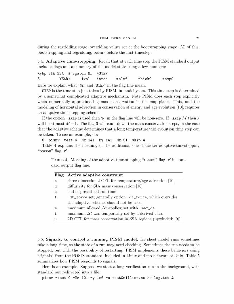
Table 4 explains the meaning of the additional one character adaptive-timestepping“reason” flag ‘r’.
Table 4. Meaning of the adaptive time-stepping “reason” flag ‘r’ in stan-dard output flag line.
Flag Active adaptive constraintc three-dimensional CFL for temperature/age advection [10]d diffusivity for SIA mass conservation [10]e end of prescribed run timef -dt_force set; generally option -dt_force, which overrides
the adaptive scheme, should not be usedm maximum allowed ∆t applies; set with -max_dt
t maximum ∆t was temporarily set by a derived classu 2D CFL for mass conservation in SSA regions (upwinded; [9])
5.5. Signals, to control a running PISM model. Ice sheet model runs sometimestake a long time, so the state of a run may need checking. Sometimes the run needs to bestopped, but with the possibility of restarting. PISM implements these behaviors using“signals” from the POSIX standard, included in Linux and most flavors of Unix. Table 5summarizes how PISM responds to signals.
Here is an example. Suppose we start a long verification run in the background, withstandard out redirected into a file:
pismv -test G -Mz 101 -y 1e6 -o testGmillion.nc >> log.txt &

22 PISM USER’S MANUAL
Table 5. Signalling PISM. pid stands for list of all identifiers of the run-ning PISM processes. The signals are POSIX but pkill is a Linux exten-sion.
Command Signal PISM behaviorkill -KILL pid SIGKILL terminate with extreme prejudice; PISM
cannot catch it and no state is savedCtrl-C typically the same for foreground process(es)kill -TERM pid SIGTERM end process(es) but PISM will save the last
model state using -o name or default namekill pid typically the samepkill -TERM pismv convenient form for MPI runs with multiple
processes needing signalkill -USR1 pid SIGUSR1 allow process(es) to continue but PISM will save
its model state at current time as “pism-year.nc”pkill -USR1 pismv convenient form for MPI runs
This run gets a Unix process id (“pid”), and we will need that number, which we assumeis “8920”. (Get it using ps or pgrep.) If we want to observe the run without stopping wesend the USR1 signal:
kill -USR1 8920
where “8920” happened to be the pid of the running PISM process. It happens that wecaught the run at year 31871.5 or so because a NetCDF file pism-31871.495239.nc isproduced. This intermediate state file can be viewed by ncview pism-31871.495239.nc.Note also that in the standard out log file log.txt the line
...
Caught signal SIGUSR1: Writing intermediate file ‘pism-31871.495239.nc’.
...
appears around time step (i.e. YEAR) 31900.Suppose, on the other hand, that the run needs to be stopped. One may use the in-
terrupt “kill -KILL 8920” for this process, which is running in the background. (Fore-ground processes can be interrupted by Ctrl-C.) This brutal method, which a processcannot catch or block, stops the process but does not allow it to save the model state.Therefore one cannot restart at the same place, nor inspect the model state. For thatability, use the TERM signal,
kill -TERM 8920
Then the PISM run is stopped and the linesCaught signal SIGTERM: exiting early.
...
Writing model state to file ‘testGmillion.nc’ ... done

PISM USER’S MANUAL 23
appear in the log file log.txt. The history global attribute testGmillion.nc recordsthe point at which the run was stopped. One can restart and finish the run by thecommand (for example)
$ pismv -test G -i testGmillion.nc -ye 1e6 \
-o testGmillion_finish.nc >> log_cont.txt &
Finally we consider a multiple process (MPI) run of PISM. Here each of the processesmust be sent the same signal at the same time. For example, consider the dialog
$ mpiexec -n 4 pismv -test C -y 100000 -o foo.nc >> log.txt &
$ ps
PID TTY TIME CMD
6761 pts/0 00:00:00 mpiexec
6762 pts/0 00:00:00 pismv
6763 pts/0 00:00:00 pismv
6764 pts/0 00:00:00 pismv
6765 pts/0 00:00:00 pismv
6770 pts/2 00:00:00 ps
$ kill -TERM 6762 6763 6764 6765
Here the kill command sent the signal to all four of the running PISM processes simulta-neously. It causes all four processes to end, and PISM writes foo.nc for possible restart.Efficiency motivates using the Linux tool pkill, which avoids the need to list process ids:
pkill -TERM pismv
See man pkill and man pgrep.
5.6. Saving snapshots of the model state. Sometimes you want to check the modelstate every 1000 years, for example. One possible solution is to run PISM for a thousandyears, have it save all the fields at the end of the run, then restart, run for anotherthousand, etc. Note this forces the adaptive time-stepping mechanism to stop exactly atmultiples of 1000 years, which may be desireable in some cases.
If saving exactly at specified times is not critical, then use of -save_to and -save_at
options is recommended. For example
$ pismr -i foo.nc -y 10000 -o output.nc -save_to snapshots.nc \
-save_at 1e3:1e3:1e4
starts a PISM evolution run, initializing from foo.nc, running for 10000 years and savingsnapshots to snapshots.nc at the first time-step after years 1000,2000,...,10000.
We use a MATLAB-style range specification, a : ∆t : b, where a,∆t, b are in years. Thetime-stepping scheme is not affected. (As a consequence we cannot guarantee producingthe exact number of snapshots requested, but this is not a problem if snapshot spacingis much greater than the length of a typical timestep. One may use -max_dt to limittime-steps if needed.)
It is also possible to save snapshots at intervals that are not equally-spaced by givingthe -save_at option a comma-separated list. For example,
$ pismr -i foo.nc -y 10000 -o output.nc -save_to snapshots.nc \

24 PISM USER’S MANUAL
-save_at 1000,1500,2000,5000
will save snapshots on the first time-step after years 1000,1500,2000 and 5000. The listgiven to the -save_at option can be at most 200 numbers long.
Another possible use of snapshots is for restarting runs on a batch system which killsjobs. Suppose that we know that we have a 8 wall-clock hours limit and a 1000 year longrun will complete in this time. We may run PISM with option -y 1500 -save_at 1000:100:1400,in which case if the job is killed before completing the 1500 year run, we can restart fromnear the last multiple of 100 years. Restarting with option -ye will hit target years.
It is possible to save snapshots to separate files using the -split_snapshots option.For example, the run above can be changed to
$ pismr -i foo.nc -y 10000 -o output.nc -save_to snapshots \
-save_at 1000,1500,2000,5000 -split_snapshots
for this purpose. This will produce files called snapshots-year.nc. This option is gen-erally faster if many snapshots are needed, apparently because of the time necessary toreopen a large file at each snapshot in the sans -split_snapshots case.
Note that tools like NCO and ncview usually behave as desired with wildcards like“snapshots-*.nc”.
5.7. Positive degree-day model. The default atmospheric climate assumption made bythe pismr and pgrn executables is that the input file will supply surface mass balance andice surface temperature in variables acab and artm, respectively. The supplied surfacemass balance acab is assumed to be the net surface balance, which is not the snowaccumulation rate when melting can occur, and it must be in units of ice-equivalentthickness per time. The supplied surface temperature artm is regarded as the meanannual surface temperature, at a point in the ice below the completion of firn processes[26]. The mass conservation equation for the ice sheet requires the surface mass balance,while the conservation of energy model requires the ice surface temperature as a boundarycondition.
These assumptions about supplied climate are not very realistic for practical glaciolog-ical observations. If the input data actually includes the annual snow-fall accumulationthen one might want to compute the surface mass balance according to some model ofhow much of the snow is transformed to ice, and how much ablates or is transported away,using a modeled time- and space-dependent temperature. An example of such a model isa positive degree day model [26], a “PDD”. The default PDD used by PISM, turned on byoption -pdd, comes from the EISMINT-Greenland intercomparison (section 8 and [53]),but it has controllable parameters.
The snow accumulation rate data should be supplied to this PDD in the input vari-able snowaccum, and should already be measured in ice-equivalent thickness per time(e.g. m s-1). The annual mean snow temperature is again the variable artm and shouldhave units K.
There are parameters controlling the seasonal temperature cycle. The positive differ-ence between the peak of seasonal temperatures and the mean (average) is called the“summer warming.” The default temperature cycle has a constant amount of summer

PISM USER’S MANUAL 25
warming, controlled by option -pdd summer warming. By default the peak of the seasonalcycle occurs on August 1, Julian day 243 (option -pdd summer peak day can overridethis). The annual mean temperature is grid-point dependent, specified by the input sur-face temperature map in variable artm, but the timing of the peak and the amount ofsummer warming are applied equally everywhere.
A PDD generally adds “white noise” to the seasonal cycle to simulate additional dailyvariability associated to the vagaries of weather. This additional random variation is quitesignificant, as the seasonal cycle may never reach the melting point but that point may bereached with some probability, in the presence of the daily variability, and thus melt mayoccur. Concretely, a normally-distributed, mean zero random temperature increment isadded to the seasonal cycle. The standard deviation of the daily variability is controlledby -pdd std dev, and defaults to 5 degrees. There is no particular assumed spatialcorrelation of daily variability.
The number of positive degree days is computed as the magnitude of the temperatureexcursion above 0◦C multiplied by the duration (in days) when it is above zero. In PISMthere are actually two methods for computing the number of positive degree days. Thefirst computes only the expected value, by the method described in [13]. This is the defaultwhen a PDD is chosen (i.e. option -pdd). The second is a monte carlo simulation of thewhite noise itself, chosen by -pdd rand. This monte carlo simulation adds the same dailyvariation at every point, though the seasonal cycle is (generally) location dependent. Ifrepeatable randomness is desired use -pdd repeatable instead of -pdd_rand.
The number of positive degree days is multiplied by a coefficient (-pdd factor snow)to compute the amount of snow melted. Of the melted snow, a fraction (-pdd refreeze)is kept as ice. This ice, plus all unmelted snow (already measured as ice-equivalent) isadded to the mass balance, unless the number of positive degree days exceeds that requiredto melt all of the snow. In this latter case, in which there are excess positive degreedays available for melting, the excess is multiplied by a coefficient (-pdd factor ice) tocompute how much ice is melted. In this case actual ablation occurs at that location.
There is an executable for testing the PDD model without invoking ice dynamics,namely pcctest. See subsection 5.12. Section 8 demonstrates the PDD model andpcctest.
5.8. Floatation criterion and mask. The most basic decision about ice dynamics madeinternally by PISM is whether to apply the “floatation criterion” to determine whetherthe ice is floating on the ocean or not. In an evolution run this decision is made at eachtime step and the result is stored in the mask.
The possible values of the mask are given in Table 6. The mask does not by itselfdetermine ice dynamics. For instance, when ice is floating (either value MASK_FLOATING
or MASK_FLOATING_OCEAN0) the usual choice for ice dynamics is SSA, but the user canchoose not to apply that model by leaving off the option -ssa.
Assuming the geometry of the ice evolves (which can be turned off by option -no mass),and assuming an ocean exists (which can be turned off by option -dry), then at each timestep the mask can change. Ice which becomes floating is marked as FLOATING while ice

26 PISM USER’S MANUAL
Table 6. The PISM mask, in combination with user options, determinesthe dynamical model.
Mask value Meaning1=SHEET ice is grounded (and only the SIA is always applied)2=DRAGGING ice is grounded (and the SSA is applied if option -ssa is given)3=FLOATING ice is floating (and the SSA is applied if option -ssa is given)7=FLOATING_OCEAN0 same as FLOATING, but the grid point was ice free ocean at
initialization of the model by -boot_from; ice with this valuewill calve off if option -ocean_kill is given.
which becomes grounded is either marked as SHEET or DRAGGING. The decision betweenSHEET or DRAGGING is made by a vote-by-neighbors scheme in the most general case. Whenboth -ssa and -super are given all grounded ice is DRAGGING, however.
5.9. Earth deformation models. Options -bed def iso and -bed def lc turn onbed deformation models. The former uses the very minimal assumption of instantaneouspointwise (i.e. independently at each point in the map plan) isostatic adjustment.
The latter is much more effective. It is based on papers by Lingle and Clark [39] and[11]. It is essentially instantaneous computationally because of use of the Fast FourierTransform to solve the relevant differential equation. Among other practical features,the rate of bed movement (uplift) is stored in the PISM output file and then is used toinitialize the next part of the run. If observed uplift data is available, it can be used alongwith -boot from to initialize the model so that it starts with the given uplift rate.
Example runs to compare these models are
$ mpiexec -n 4 pisms -eisII A -quadZ -y 8000 -o eisIIA_nobd.nc
$ mpiexec -n 4 pisms -eisII A -quadZ -bed_def_iso -y 8000 -o eisIIA_bdiso.nc
$ mpiexec -n 4 pisms -eisII A -quadZ -bed_def_lc -y 8000 -o eisIIA_bdlc.nc
Compare the topg, usurf, and dbdt variables in the resulting output files.Test H in section 6 can be used to reproduce the comparison done in [11].
5.10. Diagnostic computations. As a diagnostic example, using the EISMINT II finalstate computed in section 2, try
pismd -i eisIIA200k.nc -o eisIIA200k_diag.nc
The result is a NetCDF file eisIIA200k_diag.nc which contains the full three-dimensionalvelocity field in the scalar NetCDF variables uvel, vvel, and wvel.
The velocity field saved by pismd is the one which would be computed at the next timestep in an evolution run. That is, if we also run
pisms -eisII A -i eisIIA200k.nc -y 0 -o eisIIA200k_plus.nc
then the horizontal velocity field computed in this single time step run is the same as thatsaved in eisIIA200k_diag.nc.6
6For this example, one can use a NetCDF Operator to check that the two saved NetCDF files contain
the same vertically-averaged horizontal velocity field; just do ncdiff -v cbar . . .

PISM USER’S MANUAL 27
This diagnostic mode is most frequently associated to the modeling of ice shelves and icestreams. Subsection 9 describes using pismd to model the Ross ice shelf [41]. Verificationtests I and J, section 6, are diagnostic calculations using the SSA.
Note that the NetCDF model state saved by PISM at the end of an evolution rundoes not, by default, contain the three-dimensional velocity field. Instead, it containsjust the variables which are needed to restart the run, especially the ice geometry andtemperature field. One can also force PISM to save the full velocity field at the end ofa time-stepping run using the option -f3d. The diagnostic executable pismd saves thefull three-dimensional velocity field by default. Either way, saving the full velocity fieldroughly doubles the size of the saved NetCDF file.
5.11. Plastic till free boundary problem for ice streams; SSA as a sliding law.WARNING: The models described in this subsection are still under active development,and thus we give only a sketch.
The shallow shelf approximation (SSA) stress balance is used in PISM to describe thesliding of grounded ice and the formation of ice streams [9], as well as being used as theonly stress balance for floating ice. For the SSA with “plastic” or “Coulomb” till thelocations of ice streams is determined as part of a free boundary problem [60]. We believethat this mathematical description of ice streams, by Schoof, should be regarded as thebest known “sliding law” for the SIA [9].
Schoof’s model [60] describes emergent ice streams within a larger ice sheet and ice shelfsystem. It explains the existence of ice streams by a combination of the plastic failure ofthe till and the SSA approximation of the balance of momentum.
In PISM the user gives the options -ssa -plastic -super to turn on the use of theplastic till SSA as a sliding law. All grounded points are immediately marked as SSA(i.e. as DRAGGING). At these points a yield stress is computed from the amount of storedbasal water and from a (generally) spatially-varying till strength, tillphi in an input oroutput file. The amount of stored basal water is thermodynamically determined.
Table 7. Using the SSA stress balance in PISM.
Option combination Meaning-ssa Floating ice uses SSA, and at all points marked DRAGGING.
Basal resistance for grounded ice is plastic (see-pseudo plastic to control parameters) but usesfixed field tauc with no update.
-ssa -plastic As above, but all grounded points are forced to be DRAGGING
and tauc is updated at each time step using stored maptillphi and evolving basal melt water effective thickness bwat.
-ssa -plastic -super The recommended default sliding law. Combines SSA-computedvelocity, using plastic till, with SIA-computed velocity as in [9].
28 PISM USER’S MANUAL
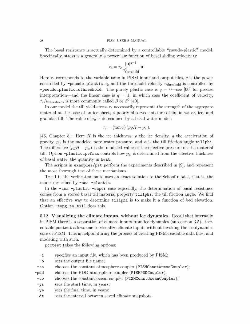
The basal resistance is actually determined by a controllable “pseudo-plastic” model.Specifically, stress is a generally a power law function of basal sliding velocity u:
τb = τc|u|q−1
uqthreshold
u.
Here τc corresponds to the variable tauc in PISM input and output files, q is the powercontrolled by -pseudo plastic q, and the threshold velocity uthreshold is controlled by-pseudo plastic uthreshold. The purely plastic case is q = 0—see [60] for preciseinterpretation—and the linear case is q = 1, in which case the coefficient of velocity,τc/uthreshold, is more commonly called β or β2 [40].
In our model the till yield stress τc necessarily represents the strength of the aggregatematerial at the base of an ice sheet, a poorly observed mixture of liquid water, ice, andgranular till. The value of τc is determined by a basal water model:
τc = (tanφ) (ρgH − pw).
[46, Chapter 8]. Here H is the ice thickness, ρ the ice density, g the acceleration ofgravity, pw is the modeled pore water pressure, and φ is the till friction angle tillphi.The difference (ρgH − pw) is the modeled value of the effective pressure on the materialtill. Option -plastic pwfrac controls how pw is determined from the effective thicknessof basal water, the quantity in bwat.
The scripts in examples/pst perform the experiments described in [9], and representthe most thorough test of these mechanisms.
Test I in the verification suite uses an exact solution to the Schoof model, that is, themodel described by -ssa -plastic.
In the -ssa -plastic -super case especially, the determination of basal resistancecomes from a stored basal till material property tillphi, the till friction angle. We findthat an effective way to determine tillphi is to make it a function of bed elevation.Option -topg to till does this.
5.12. Visualizing the climate inputs, without ice dynamics. Recall that internallyin PISM there is a separation of climate inputs from ice dynamics (subsection 3.5). Exe-cutable pcctest allows one to visualize climate inputs without invoking the ice dynamicscore of PISM. This is helpful during the process of creating PISM-readable data files, andmodeling with such.
pcctest takes the following options:
-i specifies an input file, which has been produced by PISM;-o sets the output file name;-ca chooses the constant atmosphere coupler (PISMConstAtmosCoupler);-pdd chooses the PDD atmosphere coupler (PISMPDDCoupler);-co chooses the constant ocean coupler (PISMConstOceanCoupler);-ys sets the start time, in years;-ye sets the final time, in years;-dt sets the interval between saved climate snapshots.

PISM USER’S MANUAL 29
As an example, set up an ice sheet state file and run pcctest on it:$ mpiexec -n 2 pisms -eisII A -y 10000 -o state.nc
$ pcctest -i state.nc -ca -ys 0.0 -ye 2.5 -dt 0.1 -o camovie.nc
Using pisms merely generates demonstration climate data, using EISMINT II choices[51]. pcctest extracts the surface mass balance acab and surface temperature artm fromstate.nc. It then does nothing interesting, exactly because a constant climate is used.Viewing camovie.nc we see these same values as from state.nc, in variables acab, artm,reported back to us as the time- and space-dependent climate at times ys:dt:ye. It is aboring “movie.”
The excuse for the executable pcctest becomes clearer if we use a positive degree-daymodel (subsection 5.7). The positive degree-day model uses a variable called snowaccum,and a calculation of melting, to get the surface mass balance acab. As a demonstrationhere we use an NCO (subsection 2.3) to change a variable name in state.nc. Then werun pcctest with option -pdd to invoke the PISMPDDCoupler object, which includes theparameterized PDD:$ ncrename -v acab,snowaccum state.nc restate.nc
$ pcctest -i restate.nc -pdd -ys 0.0 -ye 2.5 -dt 0.1 -o pddmovie.nc
In particular, a time-dependent view of the variable artmpdd shows the time- and space-dependent annual cycle. Onto this is added a random perturbation (normally distributedwith standard deviation of 5 degrees), but this random perturbation is not shown. Infact the PDD uses the [13] method to compute the expected number of positive degreedays. From this computation the net surface mass balance is computed, namely acab inpddmovie.nc.
See section 8 for another pcctest example.

30 PISM USER’S MANUAL
6. Verification
Two types of errors may be distinguished: modeling errors and numericalerrors. modeling errors arise from not solving the right equations. Nu-merical errors result from not solving the equations right. The assessmentof modeling errors is validation, whereas the assessment of numerical er-rors is called verification . . . Validation makes sense only after verification,otherwise agreement between measured and computed results may well befortuitous.
P. Wesseling, (2001) Principles of Computational Fluid Dynamics, pp. 560–561 [69]
Ideas. Verification is a crucial task for a code as complicated as PISM. It is the exclusivelymathematical and numerical task of checking that the predictions of the numerical codeare close to the predictions of the continuum model (the one which the numerical codeclaims to approximate). In verification there is no comparison between model output andobservations of nature. Instead, one compares exact solutions of the continuum model,in circumstance in which they are available, to the numerical approximations of thosesolutions.
See [12] and [10] for discussion of verification issues for the isothermal and thermome-chanically coupled shallow ice approximation (SIA), respectively, and for exact solutionsto these models. See [60] and [9] for an exact solution to the SSA equations for ice streamsusing a plastic till assumption. Reference [56] gives a broad discussion of verification (andvalidation) in computational fluid dynamics.
In PISM there is a separate executable pismv which is used for verification. Thesource codes which are verified by pismv are, however, exactly the same, in exactly thesame source files, as is run by the non-verification executables pismr, pisms, pgrn, etc.(In technical terms, pismv runs a derived class of the base class IceModel. All PISMexecutables run IceModel, but derived classes add bits of code, in this case the exactsolutions.)
Table 8 summarizes the many exact solutions currently available in PISM. Most of theseexact solutions are solutions of free boundary problems for partial differential equations;only Tests A, E, J, K are fixed boundary value problems. Table 9 shows how to run eachof them on minimally-refined grids (for relatively quick execution time).
Refinement. To meaningfully verify a numerical code one must go down a grid refinementpath and measure numerical error for each grid [56]. By “a refinement path” we mean thespecification of a sequence of grid cell sizes which decrease toward the refinement limitof zero size. For example, in the two spatial and one time dimension case this means asequence of triples (∆x,∆y,∆t) which decrease toward the (unreachable!) limit (0, 0, 0).By “measuring the error for each grid” we will mean computing a norm (or norms) of thedifference between the numerical solution and the exact solution. Concretely, we usuallycompute both the maximum and average numerical error of the measured quantity overthe whole grid.

PISM USER’S MANUAL 31
Table 8. Exact solutions for verification.
Test Continuum model tested Comments ReferenceA isothermal SIA, steady, [12]
flat bed, constant accumulationB isothermal SIA, flat bed, zero accum similarity soln [12, 23]C isothermal SIA, flat bed, growing accum similarity soln [12]D isothermal SIA, flat bed, oscillating accum compensatory accum [12]E isothermal SIA; as A compensatory accum [12]
but with sliding in a sectorF thermomechanically coupled SIA (mass compensatory accum [8, 10]
and energy cons.), steady, flat bed and comp heatingG thermomechanically coupled SIA; as F ditto [8, 10]
but with oscillating accumulationH bed deformation coupled with isothermal SIA joined similarity [11]I stream velocity computation using SSA (plastic till) [60, 9]J shelf velocity computation using SSA [IN PREP]K pure conduction in ice and bedrock [6]L isothermal SIA, steady, non-flat bed numerical ODE soln [IN PREP]M velocity solution for circular, constant-thickness numerical ODE soln [NOT READY]
ice shelf with grounding line and calving front
Table 9. Canonical PISM verification runs using the exact solutions listedin table 8.
Test Example invocationA pismv -test A -Mx 61 -My 61 -Mz 11 -y 25000
B pismv -test B -Mx 61 -My 61 -Mz 11 -ys 422.45 -y 25000
C pismv -test C -Mx 61 -My 61 -Mz 11 -y 15208.0
D pismv -test D -Mx 61 -My 61 -Mz 11 -y 25000
E pismv -test E -Mx 61 -My 61 -Mz 11 -y 25000
F pismv -test F -Mx 61 -My 61 -Mz 61 -y 25000
G pismv -test G -Mx 61 -My 61 -Mz 61 -y 25000
H pismv -test H -Mx 61 -My 61 -Mz 11 -y 40034 -bed_def_iso
I pismv -test I -Mx 500 -My 5 -ssa_rtol 1e-6 -ksp_rtol 1e-11
J pismv -test J -Mx 60 -My 60 -Mz 11 -ksp_rtol 1e-12
K pismv -test K -Mx 6 -My 6 -Mz 401 -Mbz 101 -y 130000
L pismv -test L -Mx 61 -My 61 -Mz 31 -y 25000
M not ready
The goal is not to see that the error is zero at any stage on the refinement path, or eventhat the error is small in a predetermined absolute sense (generally). Rather the goals are
• to see that the error is decreasing,• to measure the rate at which it is decreasing,
32 PISM USER’S MANUAL
• and to develop a realistic sense of the magnitude of numerical error, compared toother errors, in a realistic ice sheet model run.
Knowing the error decay rate may even give a prediction of how fine a grid is necessary toachieve a desired smallness for the numerical error. “Other errors” include the error fromusing the wrong (e.g. over-simplified or incorrectly-parameterized) continuum model, andalso observational or pre-processing errors present in the data used in the realistic run.
For an example of a refinement path, consider the runspismv -test B -ys 422.45 -y 25000 -Mx 31 -My 31 -Mz 11
pismv -test B -ys 422.45 -y 25000 -Mx 61 -My 61 -Mz 11
pismv -test B -ys 422.45 -y 25000 -Mx 121 -My 121 -Mz 11
pismv -test B -ys 422.45 -y 25000 -Mx 241 -My 241 -Mz 11
Here we seek to evaluate the isothermal shallow ice approximation components of PISM.The exact solution is the Halfar similarity solution [23], with zero accumulation. One spec-ifies the number of grid points when running PISM, but this is equivalent to specifying thegrid cell sizes if the overall dimensions of the computational box is fixed; see subsection 5.1.The refinement path is the sequence of triples (∆x,∆y,∆t) with ∆x = ∆y = 80, 40, 20, 10and where ∆t is determined adaptively by a stability criterion (see subsection 5.4). Notethat the vertical grid spacing ∆z is fixed because this test is isothermal. The error shouldnot depende on changing ∆z. The above four runs produce (parts of) figures 7, 8, 9, and10 of [12]. We see there that the isothermal mass conservation scheme does a reasonablejob of approximating the evolving surface. Future improvements in the numerical schememay make the error decrease faster or be smaller.
For thermocoupled tests one refines in three dimensions. For example, the runspismv -test G -max_dt 10.0 -y 25000 -Mx 61 -My 61 -Mz 61
pismv -test G -max_dt 10.0 -y 25000 -Mx 91 -My 91 -Mz 91
pismv -test G -max_dt 10.0 -y 25000 -Mx 121 -My 121 -Mz 121
pismv -test G -max_dt 10.0 -y 25000 -Mx 181 -My 181 -Mz 181
pismv -test G -max_dt 10.0 -y 25000 -Mx 241 -My 241 -Mz 241
pismv -test G -max_dt 10.0 -y 25000 -Mx 361 -My 361 -Mz 361
produced figures 13, 14, and 15 of [10]. (The last two runs, especially, require a super-computer! The 361 × 361 × 361 run involves more than 100 million unknowns, updatedat each of millions of time steps. Appropriate use -skip 10 and -quadZ accelerates suchruns. See subsection 5.)
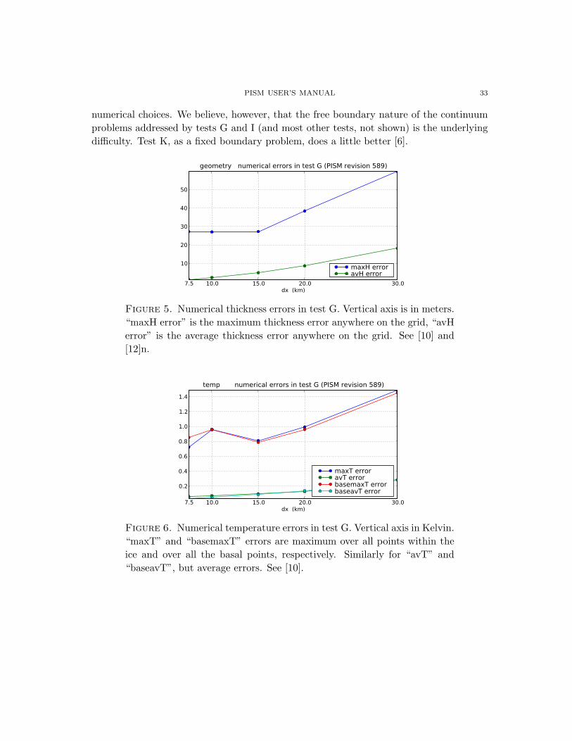
Sample verification results. Figures 5 through 9 show a sampling of the results of verifyingPISM using the tests described above. These figures were produced more-or-less automat-ically using Python scripts test/verifynow.py and test/vnreport.py. See appendixC.
It must be pointed out that, to the experienced eye, these figures do not show out-standing rates of convergence. For the errors in test G, a partial explanation comes inthe discussion of margin shape in [12], and also from presumably imperfect numericalanalysis choices. For the errors in test I, a partial explanation is low degree of smoothnesspresent for solutions in the Sobolev space used in [60], but again perhaps from imperfect
PISM USER’S MANUAL 33
numerical choices. We believe, however, that the free boundary nature of the continuumproblems addressed by tests G and I (and most other tests, not shown) is the underlyingdifficulty. Test K, as a fixed boundary problem, does a little better [6].
7.5 10.0 15.0 20.0 30.0dx (km)
10
20
30
40
50
geometry numerical errors in test G (PISM revision 589)
maxH erroravH error
Figure 5. Numerical thickness errors in test G. Vertical axis is in meters.“maxH error” is the maximum thickness error anywhere on the grid, “avHerror” is the average thickness error anywhere on the grid. See [10] and[12]n.
7.5 10.0 15.0 20.0 30.0dx (km)
0.2
0.4
0.6
0.8
1.0
1.2
1.4
temp numerical errors in test G (PISM revision 589)
maxT erroravT errorbasemaxT errorbaseavT error
Figure 6. Numerical temperature errors in test G. Vertical axis in Kelvin.“maxT” and “basemaxT” errors are maximum over all points within theice and over all the basal points, respectively. Similarly for “avT” and“baseavT”, but average errors. See [10].
34 PISM USER’S MANUAL
7.5 10.0 15.0 20.0 30.0dx (km)
0.02
0.04
0.06
0.08
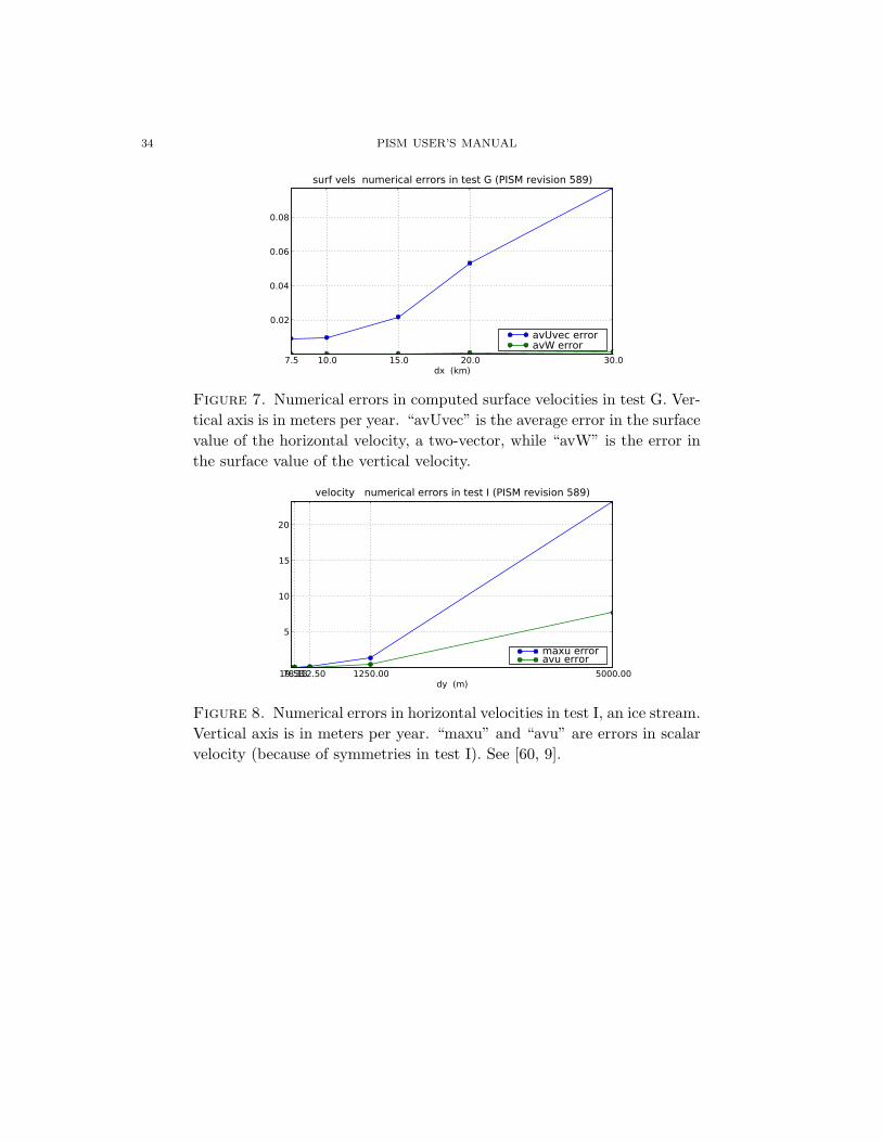
surf vels numerical errors in test G (PISM revision 589)
avUvec erroravW error
Figure 7. Numerical errors in computed surface velocities in test G. Ver-tical axis is in meters per year. “avUvec” is the average error in the surfacevalue of the horizontal velocity, a two-vector, while “avW” is the error inthe surface value of the vertical velocity.
19.5378.13312.50 1250.00 5000.00dy (m)
5
10
15
20
velocity numerical errors in test I (PISM revision 589)
maxu erroravu error
Figure 8. Numerical errors in horizontal velocities in test I, an ice stream.Vertical axis is in meters per year. “maxu” and “avu” are errors in scalarvelocity (because of symmetries in test I). See [60, 9].

PISM USER’S MANUAL 35
6.2512.50 25.00 50.00 100.00dz (m)
0.001
0.002
0.003
0.004
0.005
0.006
temp numerical errors in test K (PISM revision 589)
maxT erroravT errormaxTb erroravTb error
Figure 9. Numerical temperature errors in test K, which tests the ther-mal bedrock model. Vertical axis in Kelvin. “maxT” and “avT” are errorswithin the ice, while “maxTb” and “avTb” are in the bedrock. See [6] fora discussion.

36 PISM USER’S MANUAL
7. Simplified geometry experiments
7.1. Historical note. There have been three stages of ice sheet model intercomparisonsbased on simplified geometry experiments since the early 1990s [7].
EISMINT I [34, European Ice Sheet Modeling INiTiative]7 was the first of these andinvolved only the isothermal shallow ice approximation (SIA). Both fixed margin andmoving margin experiments were performed in EISMINT I, and various conclusions weredrawn about the several numerical schemes used in the intercomparison. EISMINT I issuperceded, however, by verification using the full variety of known exact solutions to theisothermal SIA, as shown in [12]. The “rediscovery”, since EISMINT I, of the Halfar sim-ilarity solution with zero accumulation [23] is a particular reason why good performanceon the moving margin experiment in EISMINT I is, roughly speaking, irrelevant. Forthis reason there has been no attempt to support the EISMINT I experiments in PISM,although it would be easy derived class to write.
EISMINT II [51] pointed out interesting and surprising properties of the thermocoupledSIA. References [10, 24, 25, 52, 58] each interpret the EISMINT II experiments and/ordescribe attempts to add more complete physical models to “fix” the (perceived and real)shortfalls of ice sheet model behavior on EISMINT II experiments. PISM has built-insupport for all of the published and unpublished EISMINT II experiments; these aredescribed in the next subsection.
The ISMIP (Ice Sheet Model Intercomparison Project)8 round of intercomparisons isstill ongoing at this time (2009). There are two components of ISMIP substantially com-pleted, namely HOM = Higher Order Models [49, 18] and HEINO = Heinrich Event INter-cOmparison [22]. Of these, PISM participated in HEINO, but this ability is unmaintained.We believe the continuum problem described by HEINO is not easily approximate-ablebecause of a (large) discontinuous jump in the basal velocity field. The continuum prob-lem predicts infinite vertical velocity [9, Appendix B] The same phenomenon occurs inthe EISMINT II experiment H continuum problem. Details of the numerical schemes andtheir results are irrelevant if the continuum model makes such a prediction. In essence,PISM offers the physical continuum model described in [9], an SIA/SSA hybrid, as analternative to the continuum model used in ISMIP-HEINO.
There is no current plan to support ISMIP-HOM, but comparison of shallow PISMresults to exact Stokes solutions is a goal for PISM evaluation.
A third ISMIP part is the Marine Ice Sheet Model Intercomparison Project (MISMIP).It is supported in PISM, as described in subsection 7.3.
7.2. EISMINT II in PISM. There are seven experiments described in the publishedEISMINT II writeup [51]. They are labeled A, B, C, D, F, G, and H. As specified in thewriteup, the common features of all of these experiments are:
• runs are of 200,000 years, with no prescribed time step;• runs are on a prescribed 61× 61 horizontal grid;
7See http://homepages.vub.ac.be/%7Ephuybrec/eismint.html.8See http://homepages.vub.ac.be/%7Ephuybrec/ismip.html.

PISM USER’S MANUAL 37
• the boundary conditions always have angular symmetry around the center of thegrid;• the bed is flat and does not move (there are no isostasy effects);• the temperature in the bedrock is not modeled;• only shallow ice approximation physics is included;• the change in the temperature of ice is described by the shallow approximation of
the conservation of energy [17];• thermomechanical coupling is included, both because of the temperature depen-
dence of the softness of the ice, and through the strain-heating (dissipation-heating) term in the conservation of energy equation;• the ice is cold and not polythermal [20]; and finally• though basal melt rates may be computed diagnostically, they do not affect the
evolution of the ice sheet.The experiments differ from each other in their various combinations of surface temper-ature and mass balance parameterizations. Also, experiments H and G involve basalsliding, under the dangerous SIA sliding rubric [9, Appendix B], while the others don’t.Four experiments start with zero ice (A,F,G,H), while the other experiments (B,C,D)start from the final state of experiment A.
In addition to the seven experiments published in [51], there were an additional fiveexperiments described in the EISMINT II intercomparison description [50], labeled E, I,J, K, and L. These experiments share most features, itemized above, but with the follow-ing differences. Experiment E is the same as experiment A except that the peak of theaccumulation, and also the low point of the surface temperature, are shifted by 100 kmin both x and y directions; also experiment E starts with the final state of experiment A.Experiments I and J are similar to experiment A but with non-flat topography. Experi-ments K and L are similar to experiment C but with non-flat topography. See table 10for how to run these experiments.
The vertical grid is not specified in the EISMINT II writeup. It seems that goodsimulation of the complex thermomechanically coupled conditions near the base of the icerequires relatively fine resolution there. One option in PISM is an equally-spaced grid,in which case we recommend the use of about 200 vertical levels. With a quadraticallyspaced unequal grid one can use far fewer levels. Reasonable experiment A runs, withbasal layers of thickness 25 m or less, are:
pisms -eisII A -Mx 61 -My 61 -Mz 201 -skip 5 -y 2e5 -o eisIIA_equal.nc
pisms -eisII A -Mx 61 -My 61 -Mz 61 -quadZ -skip 5 -y 2e5 -o eisIIA_quadZ.nc
The latter run is faster for memory reasons. These SIA-only simulations parallelize well,and we see speedups up to at least 30 processors for the standard 61× 61 horizontal grid.
Table 10 shows how all EISMINT II experiments are done in PISM. Experiments belowthe horizontal line in Table 10 are only documented in [50].
The EISMINT II experiments can be run with various modifications of the default set-tings. Of course the grid can be refined. For instance, a twice as fine grid in the horizontalis “-Mx 121 -My 121”. Table 11 lists some optional settings which are particular to theEISMINT II experiments.

38 PISM USER’S MANUAL
Table 10. Running the EISMINT II experiments in PISM. Replace -Mz
201 with -Mz 61 -quadZ for unequal vertical spacing. Use -skip 5 forsignificant speedup.
Command: “pisms” + Relation to experiment A-eisII A -Mx 61 -My 61 -Mz 201 -y 200000 -o eisIIA.nc
-eisII B -i eisIIA.nc -y 2e5 -o eisIIB.nc warmer-eisII C -i eisIIA.nc -y 2e5 -o eisIIC.nc less snow (lower accumulation)-eisII D -i eisIIA.nc -y 2e5 -o eisIID.nc smaller area of accumulation-eisII F -Mx 61 -My 61 -Mz 201 -y 2e5 -o eisIIF.nc colder; famous spokes [10]-eisII G -Mx 61 -My 61 -Mz 201 -y 2e5 -o eisIIG.nc sliding (regardless of temperature)-eisII H -Mx 61 -My 61 -Mz 201 -y 2e5 -o eisIIH.nc melt-temperature activated sliding-eisII E -i eisIIA.nc -y 2e5 -o eisIIE.nc shifted climate maps-eisII I -Mx 61 -My 61 -Mz 201 -y 2e5 -o eisIII.nc trough topography-eisII J -i eisIII.nc -y 2e5 -o eisIIJ.nc trough topography and less snow-eisII K -Mx 61 -My 61 -Mz 201 -y 2e5 -o eisIIK.nc mound topography-eisII L -i eisIIK.nc -y 2e5 -o eisIIL.nc mound topography and less snow
Table 11. Changing the default settings for EISMINT II.
Option Default values [expers] Units Meaning-Mmax 0.5 [ABDEFGHIK], 0.25 [CJL] m/a max value of accumulation rate-Rel 450 [ABEFGHIK], 425 [CDJL] km radial distance to equilibrium line-Sb 10−2 [all ] (m/a)/km radial gradient of accumulation rate-ST 1.67× 10⁻² [all ] K/km radial gradient of surface temperature-Tmin 238.15 [ACDEGHIJKL], K max of surface temperature
243.15[B], 223.15[F]-track_Hmelt compute effective thickness of basal melt
water (override default for EISMINT II)
Note that in PISM the height Lz of the computational box is fixed at the beginning of therun. On the other hand, changing the boundary conditions of the flow, as for instance bysetting option -Mmax to a larger than default value (see table 11), may cause the ice sheetto thicken above the Lz height. If the ice grows above the height of the computational boxthen a “Vertical grid exceeded!” or “thickness overflow in SIA velocity: ks>Mz!”error occurs. This can be fixed by restarting with a larger value for option -Lz. (Automaticrescaling of, or expansion of, the vertical grid is appropriate, but not yet implemented.)
7.3. MISMIP in PISM. This intercomparison addresses grounding line dynamics byconsidering an idealized one-dimensional stream-shelf system. The intercomparison pro-cess is described at the website
http://homepages.ulb.ac.be/~fpattyn/mismip/
Find a full text description there. These references are essential reading for understandingMISMIP results generally, and for appreciating many of the comments in this subsection.

PISM USER’S MANUAL 39
PISM’s version of MISMIP includes an attached ice shelf even though modeling theshelf is theoretically unnecessary in the MISMIP flow line case. The analysis in [62] showsthat the only effect of an ice shelf, in the flow line case, is to transfer the force imbalanceat the calving front directly to the ice column at the grounding line. But this analysis doesnot apply to ice shelves with two horizontal dimensions, of course. Real ice shelves have“buttressing” and “side drag” and other forces not present in flow line circumstances. Seethe Ross ice shelf example in section 9, for example.
We use the usual PISM ice shelf model, with two horizontal dimensions, to do MISMIP.This intercomparison therefore looks at the grounding line dynamics results from the usualPISM code, though in a highly symmetric case without side drag.
Because PISM is a model with two horizontal dimensions, we must adapt it to do aflow line problem. The flow direction for MISMIP is arbitrarily taken to be “x”. Weperiodize the cross-flow direction “y”, and use the minimum number of points in thisdirection which maintains function. This number turns out to be “-My 3”; fewer pointsthan this in the cross-flow direction confuses the finite difference scheme.
PISM has two applicable ice dynamics models corresponding to the -model 1 and-model 2 options in Table 12. Model 1 is a pure SSA model. It is “category 2” in theMISMIP classification. Model 2 combines SIA and SSA velocities as described in [9], andis “category 3” because it resolves “vertical” shear (i.e. using SIA flow).
There are many runs for a complete MISMIP intercomparison submission. There are62 runs for each model and grid choice, and there are two models and three (suggested)grid choices, so a full suite is 6× 62 = 372 runs. The finest grid runs account for all thecompute time, however. “Grid mode 2” in the MISMIP description is 1500 grid spaces inthe flow line direction, a very fine grid which imposes severe time-step restrictions on theexplicit methods in PISM. For the PISM MISMIP submission in Sept. 2008 we chose toonly submit runs for a grid with 150 (“grid mode 1”) and 600 (“grid mode 3”) grid spacesin the flow line direction. This was still 248 runs to submit, with 3 files each for a totalof 744 text files.
To do an actual MISMIP run, one uses pisms -mismip with additional options. SeeTable 12. A first run is:
$ cd examples/mismip/ (directory where some MISMIP-related scripts are)
$ pisms -mismip 1a -model 1 -step 1 -My 3 -Mz 15 -Mx 151
This will produce ASCII files ABC1_1a_M1_A1_t, ABC1_1a_M1_A1_ss, and ABC1_1a_M1_A1_f,as well as a standard NetCDF output file ABC1_1a_M1_A1.nc, in about 3 minutes. Usinga few processors speeds things up a little, and a little extra output is nice, so re-doing it:
$ mpiexec -n 4 pisms -model 1 -mismip 1a -step 1 -My 3 -Mz 15 -Mx 151 -extras
This run takes about 2 minutes on an 8 core machine. In addition to the same files asbefore, now we get an additional ASCII file ABC1_1a_M1_A1_extras. The _ss file withthickness and the _extras file with bed and surface elevation allow us to produce a figureshowing the profile for the final steady state, Figure 10:
$ ./figsMISMIP.py -p ABC1_1a_M1_A1 --extras
The script makefigs.sh will apply figsMISMIP.py to each MISMIP output in the currentdirectory.

40 PISM USER’S MANUAL
Table 12. Special MISMIP run options in PISM. Below the line are spe-cial interpretations of standard PISM options (Appendix A).
Option Default Meaning-extras if this flag is set then, once steady state is reached, surface
and bed elevation are written to an extra file with nameending “_extras”; script figsMISMIP.py reads them
-initials ABC initials to prepend to ASCII output file names-initialthk 10.0 initial thickness (m) at start of run-mismip 1a experiment number followed by sliding flag; allowed values
are 1a,1b,2a,2b,3a,3b
-model 1 model 1 is SSA only and model 2 combines SIA and SSAvelocities; see text
-no_shelf_drag flag to turn off small drag on shelves-steady_atol 1.0e-4 m/a; tolerance for steady state; criterion is
‖dH/dt‖∞ <(steady_atol value)-step 1 allowed values are {1, . . . , 9} for experiments 1 and 2, {1, . . . , 13} for
exper. 3a, and {1, . . . , 15} for exper. 3b; note typo in table 6 inmismip_4.pdf: “step 15” skipped
-try_calving flag to turn on experimental calving law which keepscalving front thickness in range [100 m, 200 m]
-Mx this option gets additional interpretation: -Mx 151 makes gridmode 1 so output files have “_M1_”; -Mx 1501 is grid mode 2(“_M2_”); any other value is grid mode 3 (“_M3_”)
-shelves_drag_too using this option has no effect because shelf drag is onby default in MISMIP; see -no_shelf_drag to turn off
MISMIP runs are done in sequence using the result of a previous run but with a stepchange in ice hardness. That is, you initialize as usual in PISM from a saved .nc file. Thenext run is
$ mpiexec -n 4 pisms -model 1 -mismip 1a -extras -step 2 -i ABC1_1a_M1_A1.nc
The result is ABC1_1a_M1_A2_t, etc.Running pisms -mismip ... with options as shown here is practical for a few ex-
amples. The script mismip.sh automates the process for the hundreds of runs in theintercomparison. Setting variables MODELRANGE and GRIDRANGE at the top of the file willmostly configure what you want. Do “./mismip.sh 4 D”, or similar, to see what callswill happen before actually starting them; “D” stands for “debug”. The script mismip.shalso illustrates how to reverse the order of steps in experiments 2a and 2b.
For significantly finer grids than mode 1, it becomes more critical to set the tolerance pa-rameters for the SSA velocity calculation. Apparently adding option -ksp_rtol 1.0e-7
is effective.The implementation of MISMIP in PISM conforms fairly closely to the intercomparison
description. However, that document specifies
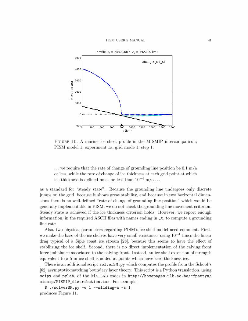
PISM USER’S MANUAL 41
Figure 10. A marine ice sheet profile in the MISMIP intercomparison;PISM model 1, experiment 1a, grid mode 1, step 1.
. . . we require that the rate of change of grounding line position be 0.1 m/aor less, while the rate of change of ice thickness at each grid point at whichice thickness is defined must be less than 10−4 m/a . . .
as a standard for “steady state”. Because the grounding line undergoes only discretejumps on the grid, because it shows great stability, and because in two horizontal dimen-sions there is no well-defined “rate of change of grounding line position” which would begenerally implementable in PISM, we do not check the grounding line movement criterion.Steady state is achieved if the ice thickness criterion holds. However, we report enoughinformation, in the required ASCII files with names ending in _t, to compute a groundingline rate.
Also, two physical parameters regarding PISM’s ice shelf model need comment. First,we make the base of the ice shelves have very small resistance, using 10−4 times the lineardrag typical of a Siple coast ice stream [28], because this seems to have the effect ofstabilizing the ice shelf. Second, there is no direct implementation of the calving frontforce imbalance associated to the calving front. Instead, an ice shelf extension of strengthequivalent to a 5 m ice shelf is added at points which have zero thickness ice.
There is an additional script solverSM.py which computes the profile from the Schoof’s[62] asymptotic-matching boundary layer theory. This script is a Python translation, usingscipy and pylab, of the Matlab codes in http://homepages.ulb.ac.be/~fpattyn/
mismip/MISMIP_distribution.tar. For example,$ ./solverSM.py -e 1 --sliding=a -s 1
produces Figure 11.

42 PISM USER’S MANUAL
Figure 11. Analytical profile for steady state of experiment 1a, grid mode1, step 1, from theory in [62]. This is a boundary layer asymptotic matchingresult, but not the exact solution to the equations solved numerically byPISM. The grounding line is at 1052.5 km. Compare Figures 10 and 13generated by PISM.
We see immediately that the PISM result does not put the grounding line in the samelocation as Schoof’s boundary layer theory. We believe the problem is with PISM’s nu-merical solution, not with that theory. More evidence that the problem is numerical canbe found by looking at the ice flux. Using ncview to examine the diagnostic variable cflx(magnitude) in ABC1_1a_M1_A1.nc we see Figure 12. This is a problem with PISM. Theflux should be a linear function. Indeed, at steady state the flux q solves a = ∇ · q wherea is the accumulation rate. In MISMIP, a is the constant 0.3 m/a, so at steady state|q| = ax, a line.
We can learn more about the problem. It turns out that the numerical flaw in the fluxalso keeps the grounding line from moving properly, we think. The problem is that thenumerical result doesn’t move the grounding line to its correct location if the ice sheet andshelf are initially 10 m as specified in MISMIP. On the other hand, the correct location forthe grounding line is also approximately a steady state for PISM numerics; the groundingline stays where you put it (compare [61] and [67]).
But solverSM.py has an option which allows the asymptotic-matching thickness resultfrom the [62] theory to be written into a NetCDF file. We can then initialize the PISMthickness from it, using -regrid_from (section 5).
The effect when we do this at higher resolution (grid mode 3 with 6km spacing, insteadof 24 km), is a step forward:
$ ./solverSM.py --Mx=601 -e 1 --sliding=a -s 1 -n SM.nc
$ mpiexec -n 4 pisms -model 1 -mismip 1a -step 1 -extras -regrid_from SM.nc \

PISM USER’S MANUAL 43
Figure 12. Numerically computed flux q = UH, where U is thevertically-averaged horizontal velocity andH the thickness, for steady stateof experiment 1a, grid mode 1, step 1. Illustrates a significant numericalproblem; it should be the dotted line, which has slope a = 0.3 m/a.
-regrid_vars H -ksp_rtol 1.0e-7 -My 3 -Mz 15 -Mx 601
The result, Figure 13, is more satisfactory. On the other hand, inspection of the flux forthis new run shows a smaller, but similarly worrying, jump in flux.
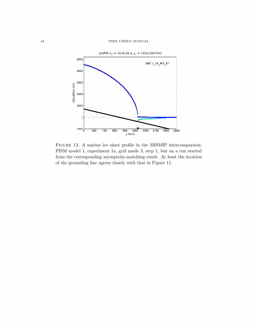
44 PISM USER’S MANUAL
Figure 13. A marine ice sheet profile in the MISMIP intercomparison;PISM model 1, experiment 1a, grid mode 3, step 1, but on a run startedfrom the corresponding asymptotic-matching result. At least the locationof the grounding line agrees closely with that in Figure 11.

PISM USER’S MANUAL 45
8. Example: Modeling the Greenland ice sheet
In this section we give an extended example of how to use PISM to model the Greenlandice sheet. We use somewhat stale data from the 1990s ice sheet modelling intercomparisonknown as EISMINT-Greenland [31, 53]9. Though based on old data, EISMINT-Greenlandserves as an excellent tutorial example.
The data for performing this experiment are freely available at
http://homepages.vub.ac.be/~phuybrec/eismint/greenland.html
The snow-fall accumulation map, ablation parameterization, surface temperature formula,surface elevation, and bedrock elevation maps are essentially as in the 1991 papers [38, 45].Note that in the ice and sea floor-core driven “forced climate” CCL3 run described belowthe ice sheet is forced by changes in temperature from the GRIP core [15] and by changesin sea level from SPECMAP [35]. A parameter-sensitivity study of a EISMINT-Greenlandtype ice sheet model is described in [54].
Substantial developments have occurred in modeling the Greenland ice sheet since theEISMINT-Greenland intercomparison. For example, the relation between a Greenlandice sheet flow model, Earth deformation under ice sheet loads, and the reconstructionof global ice loading is analyzed in [65]. The response of Greenland ice sheet models toclimate warming is addressed in [33, 32, 21], among other references.
The rest of this section is a step-by-step illustration of using PISM. The details can betyped in by hand, or the user can invoke the bash scripts preprocess.sh, bootstrap.sh,ssl2.sh, and ccl3.sh in the directory examples/eisgreen. These scripts execute thecommands in the next four subsections, respectively.
Obtaining and converting EISMINT-Greenland data. We use two Python scripts to con-vert the EISMINT-Greenland data, which is in the form of several ASCII text files, intoNetCDF files usable by PISM. The Python libraries numpy and netcdf4-python must bepresent for the scripts to work.
First, cd examples/eisgreen/ from the PISM directory, and download these text(ASCII) files from the EISMINT-Greenland web site above:
grid20-EISMINT, suaq20-EISMINT, specmap.017, sum89-92-ss09-50yr.stpOne method for the download is:
$ for name in "grid20-EISMINT" "suaq20-EISMINT" "specmap.017" "sum89-92-ss09-50yr.stp"
> do wget http://homepages.vub.ac.be/~phuybrec/eismint/$name; done
Once all four files have been downloaded, run$ ./eisgreen.py
The NetCDF file eis_green20.nc will be created from the data in grid20-EISMINT andsuaq20-EISMINT. It contains variables for the gridded latitude (lat), longitude (lon),
9EISMINT-Greenland is probably supposed to have a bedrock thermal layer and possibly a bed de-
formation model. There is no clear requirement in [53], but bedrock thermal parameter values are given.
A bedrock thermal layer is easily added using -Mbz 51, for example, and a bed deformation model with
-bed def lc.
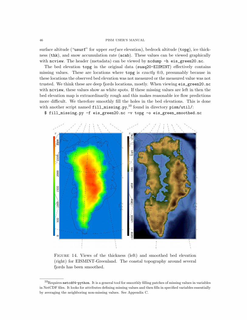
46 PISM USER’S MANUAL
surface altitude (“usurf” for upper surf ace elevation), bedrock altitude (topg), ice thick-ness (thk), and snow accumulation rate (acab). These values can be viewed graphicallywith ncview. The header (metadata) can be viewed by ncdump -h eis_green20.nc.
The bed elevation topg in the original data (suaq20-EISMINT) effectively containsmissing values. These are locations where topg is exactly 0.0, presumably because inthese locations the observed bed elevation was not measured or the measured value was nottrusted. We think these are deep fjords locations, mostly. When viewing eis_green20.nc
with ncview, these values show as white spots. If these missing values are left in then thebed elevation map is extraordinarily rough and this makes reasonable ice flow predictionsmore difficult. We therefore smoothly fill the holes in the bed elevations. This is donewith another script named fill_missing.py,10 found in directory pism/util/:
$ fill_missing.py -f eis_green20.nc -v topg -o eis_green_smoothed.nc
Figure 14. Views of the thickness (left) and smoothed bed elevation(right) for EISMINT-Greenland. The coastal topography around severalfjords has been smoothed.
10Requires netcdf4-python. It is a general tool for smoothly filling patches of missing values in variables
in NetCDF files. It looks for attributes defining missing values and then fills in specified variables essentially
by averaging the neighboring non-missing values. See Appendix C.

PISM USER’S MANUAL 47
In addition to getting the EISMINT gridded data into NetCDF format and fillingmissing values, there is an issue with Ellesmere Island. Ellesmere Island is very closeto Greenland, and so it would be possible for the modeled ice sheet to flow onto it.(This may have occurred at the last glacial maximum.) Since we don’t, however, havecorrect topography or accumulation rates for Ellesmere Island, among the downloadeddata [53], we want to prevent this from happening. Therefore special code is executed bythe PISM executable pgrn which we use below. It says that all points northwest of theline connecting the points (68.18◦E, 80.1◦N) and (62◦E, 82.24◦N) are removed from theflow simulation. The same applies to anything east of 30◦E and south of 67◦N so that theflow could not spread to the tip of Iceland (not likely anyway . . . ). The phrase “removedfrom the flow simulation” actually means that the points are marked as ice-free ocean.
Next we use the script which converts the time series data files specmap.017 andsum89-92-ss09-50yr.stp to PISM readable NetCDF form:
$ ./eiscore.py
Two NetCDF files with one-dimensional time series data are created, namely grip_dT.nc
and specmap_dSL.nc. The executable pgrn will be called with options -dTforcing and-dSLforcing for these two .nc files in the “CCL3” run below. That is, in CCL3 PISMwill read the GRIP data [15] for the surface temperature forcing and the SPECMAP data[35] for sea level forcing. Figure 15 shows the GRIP temperature offsets.
Figure 15. Change in temperature from present, from the GRIP core. Afamous graph reproduced by applying doc/gripdeltaT.py to grip dT.nc
Bootstrapping from EISMINT-Greenland data. Once the EISMINT Greenland data isobtained and converted to NetCDF, as above, “bootstrapping” can begin. By “boot-strapping” we mean the creation, by heuristics and simplified models, of the full initial

48 PISM USER’S MANUAL
conditions needed for the continuum model (differential equations describing ice dynam-ics) inside PISM.11
Table 13 shows the entire PISM output for a one model year run using option -boot_from
to “bootstrap” from file eis_green_smoothed.nc
$ pgrn -boot_from eis_green_smoothed.nc -My 141 -Mx 83 -Lz 4000 -Mz 51 \
-quadZ -skip 1 -y 1 -o green20km_y1.nc
The run takes a few seconds of real time.Let’s explain what has happened. The EISMINT-Greenland data, as with all real ice
sheet data, does not contain certain variables necessary to initialize PISM in the senseof complete initial values for time-dependent partial differential equations. For instance,the data do not include the temperature of the ice anywhere but at the surface (and onlythere by a elevation and latitude dependent formula). The data also do not include theamount of water stored in the till, for instance. These are not omissions from the data setsbut rather inevitable facts; one cannot observe ice sheets as fluids very well. ThereforePISM fills in the unknown initial conditions based on some default guesses, as indicatedby the messages in Table 13.
Note that EISMINT-Greenland specifies an 83 by 141 point grid, but you may use othernumbers for -Mx and -My if desired. In such cases the data will be linearly interpolatedonto your grid. Larger values will produce slower runs.
The option -boot_from stands for “bootstrap from”. This option is an alternative to-i (stands for “input file”) which is used for a file which has full initial conditions. Inpractice, -i is only used with a NetCDF file which was previously saved by PISM; thatis, -i is used to continue a run from a saved state.
Note the choice of the height of the computational box (“-Lz 4000”), of the numberof vertical levels (“-Mz 51”), and of a not-equally-spaced grid (“-quadZ”). The messagesto standard out show that the vertical spacing is less than 30 m near the base and morethan 130 m at the top of the computational box (where it matters less).
Regarding the temperature within the ice, bootstrapping applies an interpolation schemeto the surface temperatures and geothermal fluxes. It is based on a heuristic for theamount of downward flow in a column. Bootstrapping creates a temperature field atdepth.12
This bootstrapping mode also fills in several default values. For instance, the variablesbheatflx (geothermal flux), dbdt (bed uplift rate), and bwat (effective thickness of basalwater) were not found in the input file, whereas they would be in a saved PISM modelstate. Also, note that the EISMINT Greenland data had redundant surface elevation val-ues; PISM bootstrapping includes the computation “usurf = topg + thk” of the surfaceelevation from the ice thickness and the bed elevation.
11Section 4 will explain, once written, that “bootstrapping” is a form of inverse modeling, and that we
must inevitably do inverse modeling to do prognostic ice sheet modeling.12See the PISM Reference Manual for a formula.
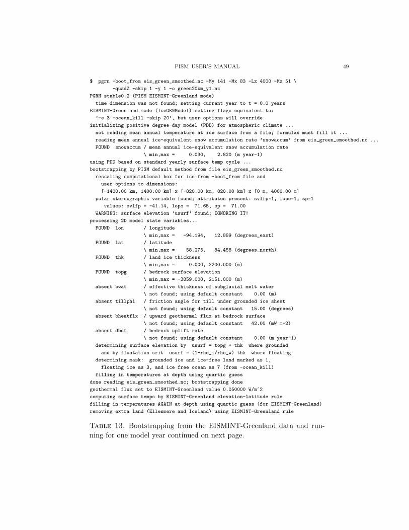
PISM USER’S MANUAL 49
$ pgrn -boot_from eis_green_smoothed.nc -My 141 -Mx 83 -Lz 4000 -Mz 51 \
-quadZ -skip 1 -y 1 -o green20km_y1.nc
PGRN stable0.2 (PISM EISMINT-Greenland mode)
time dimension was not found; setting current year to t = 0.0 years
EISMINT-Greenland mode (IceGRNModel) setting flags equivalent to:
’-e 3 -ocean_kill -skip 20’, but user options will override
initializing positive degree-day model (PDD) for atmospheric climate ...
not reading mean annual temperature at ice surface from a file; formulas must fill it ...
reading mean annual ice-equivalent snow accumulation rate ’snowaccum’ from eis_green_smoothed.nc ...
FOUND snowaccum / mean annual ice-equivalent snow accumulation rate
\ min,max = 0.030, 2.820 (m year-1)
using PDD based on standard yearly surface temp cycle ...
bootstrapping by PISM default method from file eis_green_smoothed.nc
rescaling computational box for ice from -boot_from file and
user options to dimensions:
[-1400.00 km, 1400.00 km] x [-820.00 km, 820.00 km] x [0 m, 4000.00 m]
polar stereographic variable found; attributes present: svlfp=1, lopo=1, sp=1
values: svlfp = -41.14, lopo = 71.65, sp = 71.00
WARNING: surface elevation ’usurf’ found; IGNORING IT!
processing 2D model state variables...
FOUND lon / longitude
\ min,max = -94.194, 12.889 (degrees_east)
FOUND lat / latitude
\ min,max = 58.275, 84.458 (degrees_north)
FOUND thk / land ice thickness
\ min,max = 0.000, 3200.000 (m)
FOUND topg / bedrock surface elevation
\ min,max = -3859.000, 2151.000 (m)
absent bwat / effective thickness of subglacial melt water
\ not found; using default constant 0.00 (m)
absent tillphi / friction angle for till under grounded ice sheet
\ not found; using default constant 15.00 (degrees)
absent bheatflx / upward geothermal flux at bedrock surface
\ not found; using default constant 42.00 (mW m-2)
absent dbdt / bedrock uplift rate
\ not found; using default constant 0.00 (m year-1)
determining surface elevation by usurf = topg + thk where grounded
and by floatation crit usurf = (1-rho_i/rho_w) thk where floating
determining mask: grounded ice and ice-free land marked as 1,
floating ice as 3, and ice free ocean as 7 (from -ocean_kill)
filling in temperatures at depth using quartic guess
done reading eis_green_smoothed.nc; bootstrapping done
geothermal flux set to EISMINT-Greenland value 0.050000 W/m^2
computing surface temps by EISMINT-Greenland elevation-latitude rule
filling in temperatures AGAIN at depth using quartic guess (for EISMINT-Greenland)
removing extra land (Ellesmere and Iceland) using EISMINT-Greenland rule
Table 13. Bootstrapping from the EISMINT-Greenland data and run-ning for one model year continued on next page.
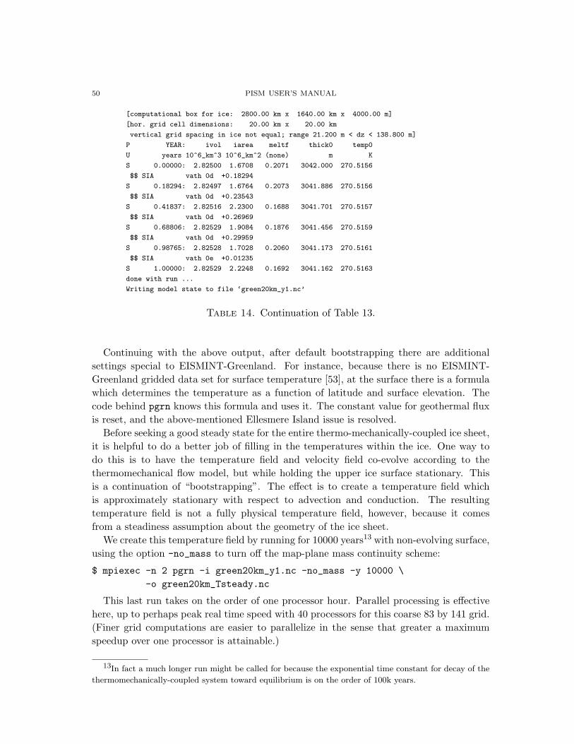
50 PISM USER’S MANUAL
[computational box for ice: 2800.00 km x 1640.00 km x 4000.00 m]
[hor. grid cell dimensions: 20.00 km x 20.00 km
vertical grid spacing in ice not equal; range 21.200 m < dz < 138.800 m]
P YEAR: ivol iarea meltf thick0 temp0
U years 10^6_km^3 10^6_km^2 (none) m K
S 0.00000: 2.82500 1.6708 0.2071 3042.000 270.5156
$$ SIA vath 0d +0.18294
S 0.18294: 2.82497 1.6764 0.2073 3041.886 270.5156
$$ SIA vath 0d +0.23543
S 0.41837: 2.82516 2.2300 0.1688 3041.701 270.5157
$$ SIA vath 0d +0.26969
S 0.68806: 2.82529 1.9084 0.1876 3041.456 270.5159
$$ SIA vath 0d +0.29959
S 0.98765: 2.82528 1.7028 0.2060 3041.173 270.5161
$$ SIA vath 0e +0.01235
S 1.00000: 2.82529 2.2248 0.1692 3041.162 270.5163
done with run ...
Writing model state to file ‘green20km_y1.nc’
Table 14. Continuation of Table 13.
Continuing with the above output, after default bootstrapping there are additionalsettings special to EISMINT-Greenland. For instance, because there is no EISMINT-Greenland gridded data set for surface temperature [53], at the surface there is a formulawhich determines the temperature as a function of latitude and surface elevation. Thecode behind pgrn knows this formula and uses it. The constant value for geothermal fluxis reset, and the above-mentioned Ellesmere Island issue is resolved.
Before seeking a good steady state for the entire thermo-mechanically-coupled ice sheet,it is helpful to do a better job of filling in the temperatures within the ice. One way todo this is to have the temperature field and velocity field co-evolve according to thethermomechanical flow model, but while holding the upper ice surface stationary. Thisis a continuation of “bootstrapping”. The effect is to create a temperature field whichis approximately stationary with respect to advection and conduction. The resultingtemperature field is not a fully physical temperature field, however, because it comesfrom a steadiness assumption about the geometry of the ice sheet.
We create this temperature field by running for 10000 years13 with non-evolving surface,using the option -no_mass to turn off the map-plane mass continuity scheme:
$ mpiexec -n 2 pgrn -i green20km_y1.nc -no_mass -y 10000 \
-o green20km_Tsteady.nc
This last run takes on the order of one processor hour. Parallel processing is effectivehere, up to perhaps peak real time speed with 40 processors for this coarse 83 by 141 grid.(Finer grid computations are easier to parallelize in the sense that greater a maximumspeedup over one processor is attainable.)
13In fact a much longer run might be called for because the exponential time constant for decay of the
thermomechanically-coupled system toward equilibrium is on the order of 100k years.

PISM USER’S MANUAL 51
The EISMINT-Greenland experiments [53] specify a positive degree day (PDD) modelwhich is automatically turned on when using the pgrn executable. (The base executablepismr requires option -pdd or -pdd_rand to turn on the PDD model.) The PDD modelis, by default, implemented by the deterministic scheme described in [13], but the usercan add option -pdd_rand to use a stochastic PDD implementation.
Running the EISMINT-Greenland steady state experiments. Now that we have initial con-ditions including a vaguely-credible temperature field, our first experiment is the steadystate run “SSL2”. This experiment uses the parameters specified in the EISMINT-Greenland description [53]. If 8 processors are used, a ten thousand model year runmight look like this:
$ mpiexec -n 8 pgrn -ssl2 -i green20km_Tsteady.nc -y 10000 -ys 0 \
-o green_SSL2_10k.nc
We can continue for another ten thousand years by
$ mpiexec -n 8 pgrn -ssl2 -i green_SSL2_10k.nc -y 10000 \
-o green_SSL2_20k.nc
And so on. The script ssh2.sh is useful to automate this, and we will now assume thatthe user actually did a run like
./ssh2.sh 2 >> out.ssl2 &
This puts the run in the background and generates a text file logging the whole run. Thewhole SSL2 run should take something like 15 processor hours to produce eleven outputfiles with names green_SSL2_Nk.nc for N = 10, . . . , 110.
Note that, by default the option -ocean_kill is set internally in pgrn. This forces allfloating ice to immediately calve off (i.e. to have thickness zero). Another default settingis -skip 20.
The SSL2 simulation is intended to go until the model reaches a “steady state”, aphrase which [53] defines as a small volume change rate, namely less than a .01% changein volume in 10,000 years.
One can look at the standard output text file by a minimal method like “less out.ssl2”.The user can more clearly see the behavior over time of the volume, area, basal melt frac-tion, and a couple of other default quantities, by generating a time series file in NetCDFform from the text (log) file coming from stdout. Then various NetCDF tools can be ap-plied to view and manipulate that file. To do this, use the Python script util/series.py,documented in Appendix C, like this:
series.py -f out.ssl2 -o ssl2.ser.nc
View ssl2.ser.nc using ncview, for instance.One sees that the volume shows a consistent growing-but-leveling-out trend, with a final
volume a bit more than 4 × 10⁶ km3. If we run the SSL2 experiment with the specified“0.01% change in 10k years” criterion, then the run ends at 110k years with a volumechange of about 0.001% between the 100k and 110k model states.
The time series for volume and melt fraction (the fraction of the base where the tem-perature is at pressure-melting) are shown in Figures 16 and 17. The volume time seriesis boring, but the melt fraction indicates something interesting: measured by basal melt

52 PISM USER’S MANUAL
fraction, the temperature field resulting from bootstrapping and relaxing the temperaturefield (above) gave a pretty good estimate of the basal melt fraction for the fully coupledsteady state.
Figure 16. Volume time series for a 110k model year EISMINT-Greenland SSL2 run; units of 106 km3.
Figure 17. Time series for the fraction of the base which is atthe pressure-melting temperature from a 110k model year EISMINT-Greenland run. See the right hand part of Figure 18 for a map of thebasal temperature.
We will use the final NetCDF file green_SSL2_110k.nc to continue the EISMINT-Greenland experiments below. The saved ice thickness, basal temperature, and vertically-averaged horizontal velocity maps are shown in Figure 18.
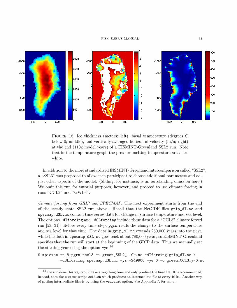
PISM USER’S MANUAL 53
Figure 18. Ice thickness (meters; left), basal temperature (degrees Cbelow 0; middle), and vertically-averaged horizontal velocity (m/a; right)at the end (110k model years) of a EISMINT-Greenland SSL2 run. Notethat in the temperature graph the pressure-melting temperature areas arewhite.
In addition to the more standardized EISMINT-Greenland intercomparison called “SSL2”,a “SSL3” was proposed to allow each participant to choose additional parameters and ad-just other aspects of the model. (Sliding, for instance, is an outstanding omission here.)We omit this run for tutorial purposes, however, and proceed to use climate forcing inruns “CCL3” and “GWL3”.
Climate forcing from GRIP and SPECMAP. The next experiment starts from the endof the steady state SSL2 run above. Recall that the NetCDF files grip_dT.nc andspecmap_dSL.nc contain time series data for change in surface temperature and sea level.The options -dTforcing and -dSLforcing include these data for a “CCL3” climate forcedrun [53, 31]. Before every time step, pgrn reads the change to the surface temperatureand sea level for that time. The data in grip_dT.nc extends 250,000 years into the past,while the data in specmap_dSL.nc goes back about 780,000 years, so EISMINT-Greenlandspecifies that the run will start at the beginning of the GRIP data. Thus we manually setthe starting year using the option -ys:14
$ mpiexec -n 8 pgrn -ccl3 -i green_SSL2_110k.nc -dTforcing grip_dT.nc \
-dSLforcing specmap_dSL.nc -ys -249900 -ye 0 -o green_CCL3_y-0.nc
14The run done this way would take a very long time and only produce the final file. It is recommended,
instead, that the user use script ccl3.sh which produces an intermediate file at every 10 ka. Another way
of getting intermediate files is by using the -save at option. See Appendix A for more.
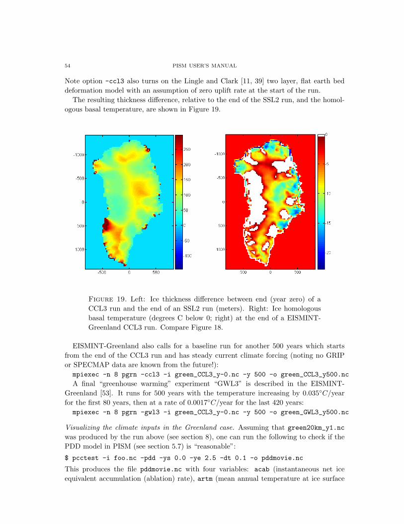
54 PISM USER’S MANUAL
Note option -ccl3 also turns on the Lingle and Clark [11, 39] two layer, flat earth beddeformation model with an assumption of zero uplift rate at the start of the run.
The resulting thickness difference, relative to the end of the SSL2 run, and the homol-ogous basal temperature, are shown in Figure 19.
Figure 19. Left: Ice thickness difference between end (year zero) of aCCL3 run and the end of an SSL2 run (meters). Right: Ice homologousbasal temperature (degrees C below 0; right) at the end of a EISMINT-Greenland CCL3 run. Compare Figure 18.
EISMINT-Greenland also calls for a baseline run for another 500 years which startsfrom the end of the CCL3 run and has steady current climate forcing (noting no GRIPor SPECMAP data are known from the future!):
mpiexec -n 8 pgrn -ccl3 -i green_CCL3_y-0.nc -y 500 -o green_CCL3_y500.nc
A final “greenhouse warming” experiment “GWL3” is described in the EISMINT-Greenland [53]. It runs for 500 years with the temperature increasing by 0.035◦C/yearfor the first 80 years, then at a rate of 0.0017◦C/year for the last 420 years:
mpiexec -n 8 pgrn -gwl3 -i green_CCL3_y-0.nc -y 500 -o green_GWL3_y500.nc
Visualizing the climate inputs in the Greenland case. Assuming that green20km_y1.nc
was produced by the run above (see section 8), one can run the following to check if thePDD model in PISM (see section 5.7) is “reasonable”:
$ pcctest -i foo.nc -pdd -ys 0.0 -ye 2.5 -dt 0.1 -o pddmovie.nc
This produces the file pddmovie.nc with four variables: acab (instantaneous net iceequivalent accumulation (ablation) rate), artm (mean annual temperature at ice surface

PISM USER’S MANUAL 55
but below firn), artmpdd (instantaneous snow temperature) and snowaccum (mean annualice-equivalent snow accumulation rate).
Variables artm and snowaccum do not evolve over time because the former is generatedfrom ice sheet geometry and latitude by the EISMINT-Greenland formulas [53], while thelatter is part of the EISMINT-Greenland data itself.
The other two variables were used to create figure 20, which shows the time-series ofthe accumulation rate (top graph) and the snow temperature (bottom graph) with themap view of the snow temperature at time 0 over it. The cross on the latter shows(approximately) the location of the point used for the time-series.
Here are two things to notice:(1) The summer peak day is in the right place. The default for this value is August
1 (day 243, at approximately 243/365 ' 0.66 year). (If it is important, the peakday can be changed using the -pdd summer peak day option; subsection 5.7).
(2) Lows of the surface mass balance rate acab correspond to positive degree-daysin the given period, because of highs of the snow temperature. Recall the snowtemperature graph does not show random daily variations. Even though it has themaximum of about 266 Kelvin, the parameterized instantaneous snow temperaturecan be above freezing. A positive value for positive degree-days is expected [13].
We can also test the surface temperature forcing code with the following command.$ pcctest -ca -i green20km_y1.nc -o dT_movie.nc \
-ys -2.5e5 -ye 0 -dt 2000 -dTforcing grip_dT.nc
The output dT_movie.nc and grip_dT.nc mentioned in section above were used to createfigure 21.
This figure shows the GRIP temperature offsets (top graph; compare to figure 15) andthe time-series of the temperature at the ice surface at a point in southern Greenland(bottom graph), confirming that the temperature offsets are used correctly.

56 PISM USER’S MANUAL
Figure 20. Time series of the surface mass balance rate and snow tem-perature. Map view on the right shows the location chosen.

PISM USER’S MANUAL 57
Figure 21. Time series of the surface temperature compared to GRIPtemperature offsets
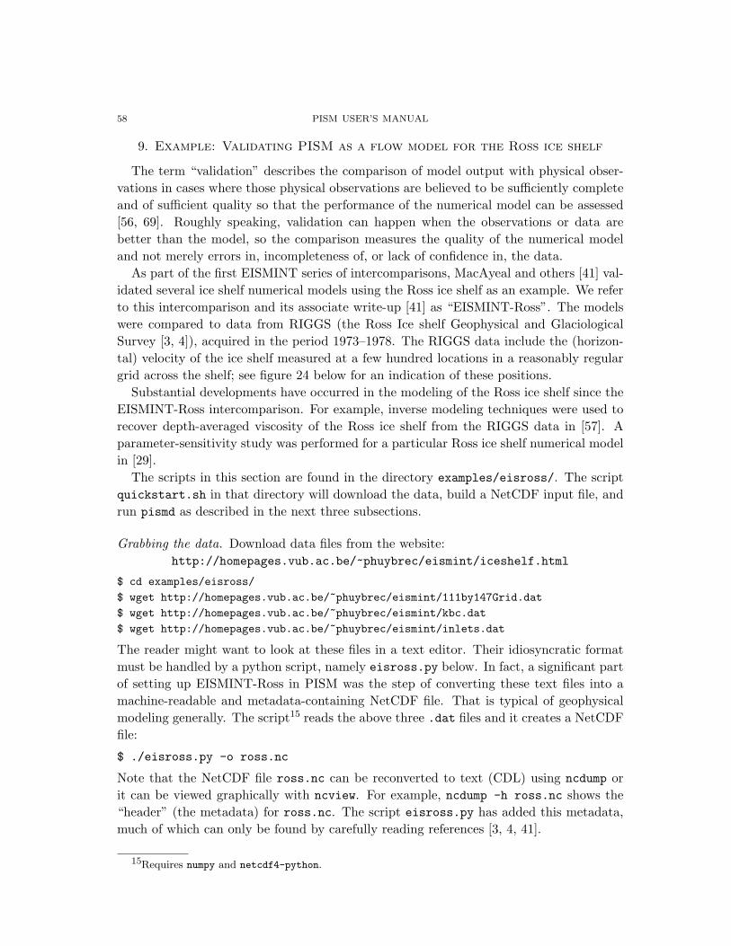
58 PISM USER’S MANUAL
9. Example: Validating PISM as a flow model for the Ross ice shelf
The term “validation” describes the comparison of model output with physical obser-vations in cases where those physical observations are believed to be sufficiently completeand of sufficient quality so that the performance of the numerical model can be assessed[56, 69]. Roughly speaking, validation can happen when the observations or data arebetter than the model, so the comparison measures the quality of the numerical modeland not merely errors in, incompleteness of, or lack of confidence in, the data.
As part of the first EISMINT series of intercomparisons, MacAyeal and others [41] val-idated several ice shelf numerical models using the Ross ice shelf as an example. We referto this intercomparison and its associate write-up [41] as “EISMINT-Ross”. The modelswere compared to data from RIGGS (the Ross Ice shelf Geophysical and GlaciologicalSurvey [3, 4]), acquired in the period 1973–1978. The RIGGS data include the (horizon-tal) velocity of the ice shelf measured at a few hundred locations in a reasonably regulargrid across the shelf; see figure 24 below for an indication of these positions.
Substantial developments have occurred in the modeling of the Ross ice shelf since theEISMINT-Ross intercomparison. For example, inverse modeling techniques were used torecover depth-averaged viscosity of the Ross ice shelf from the RIGGS data in [57]. Aparameter-sensitivity study was performed for a particular Ross ice shelf numerical modelin [29].
The scripts in this section are found in the directory examples/eisross/. The scriptquickstart.sh in that directory will download the data, build a NetCDF input file, andrun pismd as described in the next three subsections.
Grabbing the data. Download data files from the website:http://homepages.vub.ac.be/~phuybrec/eismint/iceshelf.html
$ cd examples/eisross/
$ wget http://homepages.vub.ac.be/~phuybrec/eismint/111by147Grid.dat
$ wget http://homepages.vub.ac.be/~phuybrec/eismint/kbc.dat
$ wget http://homepages.vub.ac.be/~phuybrec/eismint/inlets.dat
The reader might want to look at these files in a text editor. Their idiosyncratic formatmust be handled by a python script, namely eisross.py below. In fact, a significant partof setting up EISMINT-Ross in PISM was the step of converting these text files into amachine-readable and metadata-containing NetCDF file. That is typical of geophysicalmodeling generally. The script15 reads the above three .dat files and it creates a NetCDFfile:
$ ./eisross.py -o ross.nc
Note that the NetCDF file ross.nc can be reconverted to text (CDL) using ncdump orit can be viewed graphically with ncview. For example, ncdump -h ross.nc shows the“header” (the metadata) for ross.nc. The script eisross.py has added this metadata,much of which can only be found by carefully reading references [3, 4, 41].
15Requires numpy and netcdf4-python.
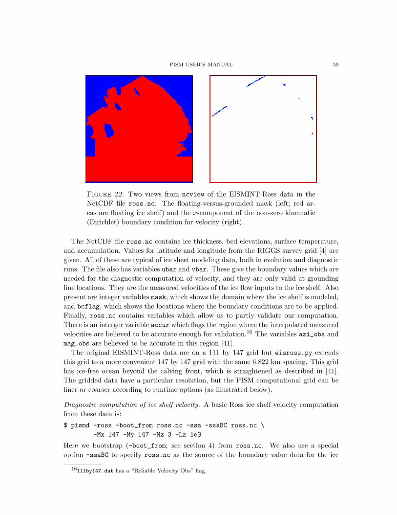
PISM USER’S MANUAL 59
Figure 22. Two views from ncview of the EISMINT-Ross data in theNetCDF file ross.nc. The floating-versus-grounded mask (left; red ar-eas are floating ice shelf) and the x-component of the non-zero kinematic(Dirichlet) boundary condition for velocity (right).
The NetCDF file ross.nc contains ice thickness, bed elevations, surface temperature,and accumulation. Values for latitude and longitude from the RIGGS survey grid [4] aregiven. All of these are typical of ice sheet modeling data, both in evolution and diagnosticruns. The file also has variables ubar and vbar. These give the boundary values which areneeded for the diagnostic computation of velocity, and they are only valid at groundingline locations. They are the measured velocities of the ice flow inputs to the ice shelf. Alsopresent are integer variables mask, which shows the domain where the ice shelf is modeled,and bcflag, which shows the locations where the boundary conditions are to be applied.Finally, ross.nc contains variables which allow us to partly validate our computation.There is an interger variable accur which flags the region where the interpolated measuredvelocities are believed to be accurate enough for validation.16 The variables azi_obs andmag_obs are believed to be accurate in this region [41].
The original EISMINT-Ross data are on a 111 by 147 grid but eisross.py extendsthis grid to a more convenient 147 by 147 grid with the same 6.822 km spacing. This gridhas ice-free ocean beyond the calving front, which is straightened as described in [41].The gridded data have a particular resolution, but the PISM computational grid can befiner or coarser according to runtime options (as illustrated below).
Diagnostic computation of ice shelf velocity. A basic Ross ice shelf velocity computationfrom these data is:
$ pismd -ross -boot_from ross.nc -ssa -ssaBC ross.nc \
-Mx 147 -My 147 -Mz 3 -Lz 1e3
Here we bootstrap (-boot_from; see section 4) from ross.nc. We also use a specialoption -ssaBC to specify ross.nc as the source of the boundary value data for the ice
16111by147.dat has a “Reliable Velocity Obs” flag.

60 PISM USER’S MANUAL
shelf equations, as mentioned in the last paragraph. The computational grid specifiedhere is the 6.822 km data grid in EISMINT-Ross with 147 grid points in each direction.The maximum thickness of the ice is 874 m so we choose a height for the computationalbox (-Lz) large enough to contain the ice. Note that using a small number of verticallevels (-Mz 11) is reasonable because the EISMINT-Ross intercomparison specifies thatthe temperature at each depth is just the surface temperature [41]. In fact there is nothermocoupling issue because the ice hardness used here is constant.
At the end of this run the computed velocity field is compared to the interpolatedobserved velocities stored in ross.nc. The value called “average relative error in vectorvel” is most relevant. A value of 0.07 here means that the averaged absolute differencebetween the computed and the observed velocity, in the “accurate” region, is 7%.
The output file unnamed_diag.nc contains vertically-averaged horizontal speed in thevariable cbar. Viewing that variable will show a picture like the one on the cover page ofthis User’s Manual, and like that in figure 23.
Figure 23. Computed horizontal ice speed of the Ross ice shelf. Colorgives velocity in m/a; see scale.
There are many variations on this basic “pismd -ross” run above. First of all one canget more information during the run by adding diagnostic viewers and a more complete(verbose) report to standard out:
$ pismd -ross -boot_from ross.nc -ssa -ssaBC ross.nc \
-Mx 147 -My 147 -Mz 3 -Lz 1e3 -d cnmu -verbose -pause 10
Secondly one might want to do the run in parallel and do it on a finer grid. For example,
$ mpiexec -n 4 pismd -ross -boot_from ross.nc -ssa -ssaBC ross.nc \
-Mx 201 -My 201 -Mz 3 -Lz 1e3

PISM USER’S MANUAL 61
The result is very similar, as it should be. On the other hand, since the data is only on a6.8 km grid we expect no added accuracy on this new 5km grid.
Alternately one might want to experiment with different values of the hardness pa-rameter. Its default value is B = 1.9 × 10⁸ Pa s1/3 as in [41]. We can also use smaller(more severe) tolerances for the nonlinear iteration (-ssa rtol) and the linear iteration(-ksp rtol) to get more confidence in the numerical scheme:
$ pismd -ross -boot_from ross.nc -ssaBC ross.nc -Mx 147 -My 147 -Lz 1000 \
-Mz 11 -ssa -ice_type custom -ice_custom_hardness 1.8e8 \
-o ross_out_1p8.nc -ssa_rtol 1e-6 -ksp_rtol 1e-10
Table 15 lists some of the options which are useful for this kind of diagnostic velocitycomputation.
Table 15. Non-obvious options available and/or recommended withpismd -ross.
Option Explanation/Comments-d cnmu a good way to see what is going on-mato foo -matv cnmuvH writes some model results to
Matlab-readable file foo.m
-pause N pause for N seconds when refreshing viewers-ross only use with executable pismd
-verbose 4 shows information on nonlinear iteration and Krylov solveand parameters related to solving the ice shelf equations
Comparison to RIGGS data. The file riggs_clean.dat is a cleaned-up version of theoriginal RIGGS data [4, 3]. (See README for more explanation on this RIGGS data.) Toconvert this data to a NetCDF file, as needed next, do
./eisriggs.py -o riggs.nc
A file riggs.nc will be created. This data is one-dimensional; it is just a lists of valueswhich have an index dimension count in the NetCDF file riggs.nc.
Now, pismd -ross can read this data and compute a χ2 statistic comparing computedPISM output to the data:$ pismd -ross -boot_from ross.nc -ssaBC ross.nc -Mx 147 -My 147 -Lz 1000 -Mz 3 \
-ssa -riggs riggs.nc
PISMD stable0.2 (diagnostic velocity computation mode)
. . .
initializing EISMINT-Ross ice shelf velocity computation ...
. . .
maximum computed speed in ice shelf is 1364.654 (m/a)
. . .
comparing to RIGGS data in riggs.nc ...
Chi^2 statistic for computed results compared to RIGGS is 3637.016
Writing model state, with full 3D velocities, to file ‘unnamed_diag.nc’
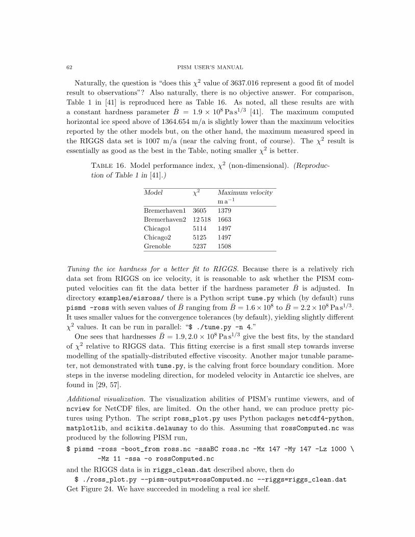
62 PISM USER’S MANUAL
Naturally, the question is “does this χ2 value of 3637.016 represent a good fit of modelresult to observations”? Also naturally, there is no objective answer. For comparison,Table 1 in [41] is reproduced here as Table 16. As noted, all these results are witha constant hardness parameter B = 1.9 × 10⁸ Pa s1/3 [41]. The maximum computedhorizontal ice speed above of 1364.654 m/a is slightly lower than the maximum velocitiesreported by the other models but, on the other hand, the maximum measured speed inthe RIGGS data set is 1007 m/a (near the calving front, of course). The χ2 result isessentially as good as the best in the Table, noting smaller χ2 is better.
Table 16. Model performance index, χ2 (non-dimensional). (Reproduc-
tion of Table 1 in [41].)
Model χ2 Maximum velocity
m a−1
Bremerhaven1 3605 1379Bremerhaven2 12 518 1663Chicago1 5114 1497Chicago2 5125 1497Grenoble 5237 1508
Tuning the ice hardness for a better fit to RIGGS. Because there is a relatively richdata set from RIGGS on ice velocity, it is reasonable to ask whether the PISM com-puted velocities can fit the data better if the hardness parameter B is adjusted. Indirectory examples/eisross/ there is a Python script tune.py which (by default) runspismd -ross with seven values of B ranging from B = 1.6× 10⁸ to B = 2.2× 10⁸ Pa s1/3.It uses smaller values for the convergence tolerances (by default), yielding slightly differentχ2 values. It can be run in parallel: “$ ./tune.py -n 4.”
One sees that hardnesses B = 1.9, 2.0 × 10⁸ Pa s1/3 give the best fits, by the standardof χ2 relative to RIGGS data. This fitting exercise is a first small step towards inversemodelling of the spatially-distributed effective viscosity. Another major tunable parame-ter, not demonstrated with tune.py, is the calving front force boundary condition. Moresteps in the inverse modeling direction, for modeled velocity in Antarctic ice shelves, arefound in [29, 57].
Additional visualization. The visualization abilities of PISM’s runtime viewers, and ofncview for NetCDF files, are limited. On the other hand, we can produce pretty pic-tures using Python. The script ross_plot.py uses Python packages netcdf4-python,matplotlib, and scikits.delaunay to do this. Assuming that rossComputed.nc wasproduced by the following PISM run,$ pismd -ross -boot_from ross.nc -ssaBC ross.nc -Mx 147 -My 147 -Lz 1000 \
-Mz 11 -ssa -o rossComputed.nc
and the RIGGS data is in riggs_clean.dat described above, then do$ ./ross_plot.py --pism-output=rossComputed.nc --riggs=riggs_clean.dat
Get Figure 24. We have succeeded in modeling a real ice shelf.
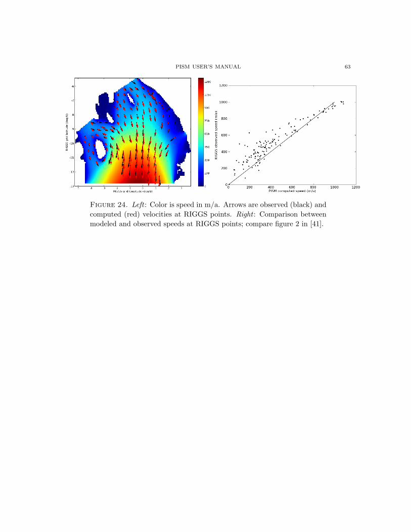
PISM USER’S MANUAL 63
Figure 24. Left : Color is speed in m/a. Arrows are observed (black) andcomputed (red) velocities at RIGGS points. Right : Comparison betweenmodeled and observed speeds at RIGGS points; compare figure 2 in [41].
64 PISM USER’S MANUAL
References
[1] S. Balay and eight others, PETSc Users Manual, Tech. Rep. ANL-95/11 - Revision 2.3.2, Argonne
National Laboratory, 2006. http://www.mcs.anl.gov/petsc/petsc-as/snapshots/petsc-current/
docs/manual.pdf.
[2] J. L. Bamber, D. G. Vaughan, and I. Joughin, Widespread complex flow in the interior of the
Antarctic ice sheet, Science, 287 (2000), pp. 1248–1250.
[3] C. R. Bentley, Glaciological studies on the Ross Ice Shelf, Antarctica, 1973–1978, Antarctic Re-
search Series, 42 (1984), pp. 21–53.
[4] , The Ross Ice shelf Geophysical and Glaciological Survey (RIGGS): Introduction and summary
of measurments performed, Antarctic Research Series, 42 (1984), pp. 1–20.
[5] H. Blatter, Velocity and stress fields in grounded glaciers: a simple algorithm for including devia-
toric stress gradients, J. Glaciol., 41 (1995), pp. 333–344.
[6] E. Bueler, An exact solution to the temperature equation in a column of ice and bedrock. preprint
arXiv:0710.1314, 2007.
[7] E. Bueler, Lessons from the short history of ice sheet model intercomparison, The Cryosphere Dis-
cussions, 2 (2008), pp. 399–412. http://www.the-cryosphere-discuss.net/2/399/2008/.
[8] E. Bueler and J. Brown, On exact solutions and numerics for cold, shallow, and thermocoupled
ice sheets. preprint arXiv:physics/0610106, 2006.
[9] , The shallow shelf approximation as a “sliding law” in a thermodynamically coupled ice sheet
model, J. Geophys. Res. (Earth Surface, (2009). accepted; preprint at arxiv.org/abs/0810.3449.
[10] E. Bueler, J. Brown, and C. Lingle, Exact solutions to the thermomechanically coupled shallow
ice approximation: effective tools for verification, J. Glaciol., 53 (2007), pp. 499–516.
[11] E. Bueler, C. S. Lingle, and J. A. Kallen-Brown, Fast computation of a viscoelastic deformable
Earth model for ice sheet simulation, Ann. Glaciol., 46 (2007), pp. 97–105.
[12] E. Bueler, C. S. Lingle, J. A. Kallen-Brown, D. N. Covey, and L. N. Bowman, Exact
solutions and numerical verification for isothermal ice sheets, J. Glaciol., 51 (2005), pp. 291–306.
[13] R. Calov and R. Greve, Correspondence: A semi-analytical solution for the positive degree-day
model with stochastic temperature variations, J. Glaciol, 51 (2005), pp. 173–175.
[14] N. Calvo et al., On a doubly nonlinear parabolic obstacle problem modelling ice sheet dynamics,
SIAM J. Appl. Math., 63 (2002a), pp. 683–707.
[15] W. Dansgaard and ten others, Evidence for general instability of past climate from a 250-kyr
ice-core record, Nature, 364 (1993), pp. 218–220.
[16] EPICA community members, Eight glacial cycles from an Antarctic ice core, Nature, 429 (2004),
pp. 623–628. doi: 10.1038/nature02599.
[17] A. C. Fowler, Mathematical Models in the Applied Sciences, Cambridge Univ. Press, 1997.
[18] O. Gagliardini and T. Zwinger, The ismip-hom benchmark experiments performed using
the finite-element code elmer, The Cryosphere Discussions, 2 (2008), pp. 75–109. http://www.
the-cryosphere-discuss.net/2/75/2008/.
[19] D. L. Goldsby and D. L. Kohlstedt, Superplastic deformation of ice: experimental observations,
J. Geophys. Res., 106 (2001), pp. 11017–11030.
[20] R. Greve, A continuum–mechanical formulation for shallow polythermal ice sheets, Phil. Trans. Royal
Soc. London A, 355 (1997), pp. 921–974.
[21] R. Greve, On the response of the Greenland ice sheet to greenhouse climate change, Climatic Change,
46 (2000), pp. 289–303.
[22] R. Greve, R. Takahama, and R. Calov, Simulation of large-scale ice-sheet surges: The ISMIP-
HEINO experiments, Polar Meteorol. Glaciol., 20 (2006), pp. 1–15.
[23] P. Halfar, On the dynamics of the ice sheets 2, J. Geophys. Res., 88 (1983), pp. 6043–6051.
[24] R. C. A. Hindmarsh, Thermoviscous stability of ice-sheet flows, J. Fluid Mech., 502 (2004), pp. 17–
40.
PISM USER’S MANUAL 65
[25] , Stress gradient damping of thermoviscous ice flow instabilities, J. Geophys. Res., 111 (2006).
doi:10.1029/2005JB004019.
[26] R. Hock, Glacier melt: a review of processes and their modelling, Prog. Phys. Geog., 29 (2005),
pp. 362–391.
[27] R. Hooke, Flow law for polycrystalline ice in glaciers: comparison of theoretical predictions, labora-
tory data, and field measurements, Rev. Geophys. Space. Phys., 19 (1981), pp. 664–672.
[28] C. L. Hulbe and D. R. MacAyeal, A new numerical model of coupled inland ice sheet, ice stream,
and ice shelf flow and its application to the West Antarctic Ice Sheet, J. Geophys. Res., 104 (1999),
pp. 25349–25366.
[29] A. Humbert, R. Greve, and K. Hutter, Parameter sensitivity studies for the ice flow of the Ross
Ice Shelf, Antarctica, J. Geophys. Res., 110 (2005). doi:10.1029/2004JF000170.
[30] K. Hutter, Theoretical Glaciology, D. Reidel, 1983.
[31] P. Huybrechts, Report of the Third EISMINT Workshop on Model Intercomparison.
homepages.vub.ac.be/∼phuybrec/pdf/EISMINT3.Huyb.1998.pdf; 120 pages, 1998.
[32] P. Huybrechts, Sea-level changes at the LGM from ice-dynamic reconstructions of the Greenland
and Antarctic ice sheets during the glacial cycles, Quat. Sci. Rev., 21 (2002), pp. 203–231.
[33] P. Huybrechts and J. de Wolde, The dynamic response of the Greenland and Antarctic ice sheets
to multiple-century climatic warming, J. Climate, 12 (1999), pp. 2169–2188.
[34] P. Huybrechts et al., The EISMINT benchmarks for testing ice-sheet models, Ann. Glaciol., 23
(1996), pp. 1–12.
[35] J. Imbrie and eight others, The orbital theory of Pleistocene climate: Support from a revised
chronology of the marine δ 18O record, in Milankovitch and Climate: Understanding the Response to
Astronomical Forcing, D. Reidel, 1984, pp. 269–305.
[36] I. Joughin, M. Fahnestock, S. Ekholm, and R. Kwok, Balance velocities of the Greenland ice
sheet, Geophysical Research Letters, 24 (1997), pp. 3045–3048.
[37] I. Joughin, M. Fahnestock, D. MacAyeal, J. L. Bamber, and P. Gogineni, Observation and
analysis of ice flow in the largest Greenland ice stream, J. Geophys. Res., 106 (2001), pp. 34021–34034.
[38] A. Letreguilly, P. Huybrechts, and N. Reeh, Steady-state characteristics of the Greenland ice
sheet under different climates, J. Glaciol., 37 (1991), pp. 149–157.
[39] C. S. Lingle and J. A. Clark, A numerical model of interactions between a marine ice sheet and the
solid earth: Application to a West Antarctic ice stream, J. Geophys. Res., 90 (1985), pp. 1100–1114.
[40] D. R. MacAyeal, Large-scale ice flow over a viscous basal sediment: theory and application to ice
stream B, Antarctica, J. Geophys. Res., 94 (1989), pp. 4071–4087.
[41] D. R. MacAyeal, V. Rommelaere, P. Huybrechts, C. Hulbe, J. Determann, and C. Ritz,
An ice-shelf model test based on the Ross ice shelf, Ann. Glaciol., 23 (1996), pp. 46–51.
[42] M. W. Mahaffy, A three–dimensional numerical model of ice sheets: tests on the Barnes Ice Cap,
Northwest Territories, J. Geophys. Res., 81 (1976), pp. 1059–1066.
[43] L. W. Morland, Unconfined ice-shelf flow, in Dynamics of the West Antarctic ice sheet, C. J. van der
Veen and J. Oerlemans, eds., Kluwer Academic Publishers, 1987, pp. 99–116.
[44] L. W. Morland and R. Zainuddin, Plane and radial ice-shelf flow with prescribed temperature
profile, in Dynamics of the West Antarctic ice sheet, C. J. van der Veen and J. Oerlemans, eds.,
Kluwer Academic Publishers, 1987, pp. 117–140.
[45] A. Ohmura and N. Reeh, New precipitation and accumulation maps for Greenland, J. Glaciol., 37
(1991), pp. 140–148.
[46] W. S. B. Paterson, The Physics of Glaciers, Pergamon, 3rd ed., 1994.
[47] W. S. B. Paterson and W. F. Budd, Flow parameters for ice sheet modeling, Cold Reg. Sci.
Technol., 6 (1982), pp. 175–177.
[48] F. Pattyn, A new three-dimensional higher-order thermomechanical ice sheet model: Basic sensi-
tivity, ice stream development, and ice flow across subglacial lakes, J. Geophys. Res., 108 (2003),
pp. EPM 4–1. Doi:10.1029/2002JB002329, CiteID 2382.
66 PISM USER’S MANUAL
[49] F. Pattyn et al., Benchmark experiments for higher-order and full Stokes ice sheet models (ISMIP-
HOM), The Cryosphere Discussions, 2 (2008), pp. 111–151. http://www.the-cryosphere-discuss.
net/2/111/2008/.
[50] A. Payne, EISMINT: Ice sheet model intercomparison exercise phase two. Proposed simplified geom-
etry experiments. homepages.vub.ac.be/∼phuybrec/eismint/thermo-descr.pdf, 1997.
[51] A. Payne et al., Results from the EISMINT model intercomparison: the effects of thermomechanical
coupling, J. Glaciol., 153 (2000), pp. 227–238.
[52] A. J. Payne and D. J. Baldwin, Analysis of ice–flow instabilities identified in the EISMINT inter-
comparison exercise, Ann. Glaciol., 30 (2000), pp. 204–210.
[53] C. Ritz, EISMINT Intercomparison Experiment: Comparison of existing Greenland models.
homepages.vub.ac.be/∼phuybrec/eismint/greenland.html, 1997.
[54] C. Ritz, A. Fabre, and A. Letreguilly, Sensitivity of a Greenland ice sheet model to ice flow and
ablation parameters: consequences for the evolution through the last glacial cycle, Climate Dyn., 13
(1997), pp. 11–24.
[55] C. Ritz, V. Rommelaere, and C. Dumas, Modeling the evolution of Antarctic ice sheet over the last
420,000 years: Implications for altitude changes in the Vostok region, J. Geophys. Res., 106 (2001),
pp. 31943–31964.
[56] P. Roache, Verification and Validation in Computational Science and Engineering, Hermosa Pub-
lishers, Albuquerque, New Mexico, 1998.
[57] V. Rommelaere and D. R. MacAyeal, Large-scale rheology of the Ross Ice Shelf, Antarctica,
computed by a control method, Ann. Glaciol., 24 (1997), pp. 43–48.
[58] F. Saito, A. Abe-Ouchi, and H. Blatter, European Ice Sheet Modelling Initiative (EIS-
MINT) model intercomparison experiments with first-order mechanics, J. Geophys. Res., 111 (2006).
doi:10.1029/2004JF000273.
[59] , An improved numerical scheme to compute horizontal gradients at the ice-sheet margin: its
effect on the simulated ice thickness and temperature, Ann. Glaciol., 46 (2007), pp. 87–96.
[60] C. Schoof, A variational approach to ice stream flow, J. Fluid Mech., 556 (2006), pp. 227–251.
[61] , Ice sheet grounding line dynamics: Steady states, stability, and hysteresis, J. Geophys. Res.,
112 (2007). F03S28, doi:10.1029/2006JF000664.
[62] , Marine ice-sheet dynamics. Part 1. The case of rapid sliding, J. Fluid Mech., 573 (2007),
pp. 27–55.
[63] , Coulomb friction and other sliding laws in a higher order glacier flow model, Math. Models
Methods Appl. Sci. (M3AS), (to appear).
[64] C. Schoof and R. Hindmarsh, Thin-film flows with wall slip: an asymptotic analysis of higher
order glacier flow models, J. Fluid Mech., (submitted).
[65] L. Tarasov and W. R. Peltier, Greenland glacial history and local geodynamic consequences,
Geophys. J. Int., 150 (2002), pp. 198–229.
[66] L. N. Trefethen, Spectral Methods in MATLAB, SIAM Press, 2000.
[67] A. Vieli and A. J. Payne, Assessing the ability of numerical ice sheet models to simulate grounding
line migration, J. Geophysical Research, 110 (2005). F01003, doi:10.1029/2004JF000202.
[68] M. Weis, R. Greve, and K. Hutter, Theory of shallow ice shelves, Continuum Mech. Thermodyn.,
11 (1999), pp. 15–50.
[69] P. Wesseling, Principles of Computational Fluid Dynamics, Springer-Verlag, 2001.
PISM USER’S MANUAL 67
Appendix A. PISM command line options
Much of the behavior of PISM can be set at the command line by options. For example,the command
$ pismv -test C -Mx 61 -e 1.2 -o foo.nc
includes four options “-test”, “-Mx”, “-e”, and “-o”, The first of these options includesa single character argument, the second an integer argument, the third a floating pointargument, and the fourth has a string argument.
The format of the option documentation below is“-optionname [A][B only ]: Description.”
Here “A” is the default value and “B” is a list of the allowed executables. The optionapplies to all executables (pismr, pisms, pismv) unless the allowed executables are specif-ically stated by giving “[B only ]”.
As PISM is a PETSc program [1], all PETSc options are available as well. The lastsubsection A.2 recalls some of these PETSc options.
The Index on page 86 contains an alphabetical list of options.
A.1. List of PISM options.
Options controlling model run length/start/end.
-y [1000]: Number of model years to run.
-ye : Model year at which to end the run. The default value is the start year (-ysor initialized model time from file) plus the default or given (-y) run length. If both -ys
and -ye are used then the run length is set to the difference. Using all three of -ys, -yand -ys is not allowed.
-ys : Model year at which to start the run. Also resets the model time, ignoring anytime in the input file.
Options controlling the (spatial) computational grid and box.
-chebZ : Specify Chebyshev-spaced grid in the vertical. This grid is extremely finenear the base, and choice -quadZ is probably better justified (by current understanding ofthe thermocoupling and age problems) than is -chebZ. Use only in combination with theoption -boot_from or with executables like pisms and pismv that initialize the grid fromformulas. (It will not work with -i.) See subsection 5.2. For a detailed description of thespacing of the grid, see the documentation on IceGrid::compute_vertical_levels()
in the PISM Reference Manual.
-Lx : The x direction half-width of the computational box, in kilometers. See section5.
-Ly : The y direction half-width of the computational box, in kilometers. See section5.

68 PISM USER’S MANUAL
-Lz : The height of the computational box for the ice (excluding the bedrock thermalmodel part). See section 5.
-Mbz [1]: Number of grid points in the bedrock for the bedrock thermal model. Thehighest grid point corresponds to the base of the ice z = 0, and so Mbz> 1 is required toactually have bedrock thermal model. Note this option is unrelated to the bed deformationmodel (glacial isostasy model); see option -bed_def for that.
-Mx [61]: Number of grid points in x horizontal direction.
-My [61]: Number of grid points in y horizontal direction.
-Mz [31]: Number of grid points in z (vertical) direction.
-quadZ : Specify quadratically-spaced grid in the vertical. The spacing near the baseis about four times finer than it would be with equal spacing for the same value of Mz, whilethe spacing near the top is correspondingly coarser. Use only in combination with theoption -boot_from or with executables like pisms and pismv that initialize the grid fromformulas. (It will not work with -i.) See subsection 5.2. For a detailed description of thespacing of the grid, see the documentation on IceGrid::compute_vertical_levels()
in the PISM Reference Manual.
Options turning on and off major physical models.
-bed def iso : Compute bed deformations by simple pointwise isostasy. Assumesthat the bed at the starting time is in equilibrium with the load so the bed elevation isequal to the starting bed elevation minus a multiple of the increase in ice thickness fromthe starting time, roughly: b(t, x, y) = b(0, x, y)− f [H(t, x, y)−H(0, x, y)]. Here f is thedensity of ice divided by the density of the mantle. See Test H in Verification section.
-bed def lc : Compute bed deformations, caused by the changing load of the ice,using a viscoelastic earth model. Uses the model and computational technique describedin [11], based on the continuum model in [39].
-float kill : If ice is (or becomes) floating then it is set to thickness zero. Thisis calving at the grounding line.
-hold tauc : Keep the current values of the till yield stress τc. That is, do notupdate them by the default model using the stored basal melt water. Only effective if-ssa and -plastic are also set. See documentation of option -plastic for a descriptionof the till yield stress model.
-no mass : Forces PISM to not change the ice thickness. No time steps of the massconservation equation are computed.
-no temp : Force PISM to not change temperature or age values within the ice. Notime steps of the energy conservation and age equations are computed.
-ocean kill : If used with input from a NetCDF initialization file which has ice-free ocean mask (value MASK_FLOATING_OCEAN0= 7), will zero out ice thicknesses in areasthat were ice-free ocean at time zero. This is calving at the location of the original calvingfront. Has no effect when used in conjunction with -no_mass.
PISM USER’S MANUAL 69
-pdd : Turns on the positive degree day model (which is off by default for pismr,pisms, and pismv). Use the method described in [13], which computes the expectednumber of positive degree days. See subsection 5.7.
-plastic : Use Schoof’s plastic till model for ice streams at all grounded points onthe ice sheet. Must be used along with -ssa to turn on the solution of the SSA (shallowshelf approximation). See subsection 5.11. See options -plastic_reg, -plastic_c0,-plastic_phi, and -plastic_pwfrac, all of which control the plastic till model in variousways.
Indeed, we describe the role of the parameters for the plastic till model as follows: Theeffective pressure N on the till is
N = P − p = (1− (pwfrac)λ)P
where P = ρgH is the overburden or hydrostatic pressure at the base (see Paterson [46],pp. 168–169) and p = (pwfrac)λP is the pore water pressure in the till. Here λ is a purenumber, 0 ≤ λ ≤ 1, measuring the amount of available basal water. In particular, λ = 0if the base is frozen, while λ is a linear function of the stored basal melt water (see -d L),up to the fixed maximum amount of stored basal melt water. Thus our model says thatwhen there is a lot (the maximum) amount of available basal water, p = (pwfrac)P ; thedefault value for pwfrac is 0.95.
Note that Paterson gives this formula for the till yield stress
τc = c0 + µN, µ = tanφ,
while Schoof [60] formula (2.4) gives this one
τc = µN,
with zero till cohesion. We allow a positive till cohesion, though the default is zero, andwe describe µ as the tangent of the friction angle φ.
-ssa : Use the equations of the shallow shelf approximation [40, 43, 60, 68] for iceshelves and dragging ice shelves (i.e. ice streams) where so-indicated by the mask. Toview the mask use -d m. See also -plastic and -super. See also -dontreadSSAvels.
-super : Combine the velocity fields from the SIA and SSA models as in [9]. Onlyeffective if used with -ssa.
Options controlling input and output behavior of PISM.
A.1.1. File input and output from PISM.
-boot from : The model can be “bootstrapped” from certain NetCDF files usingless than the full initial values for the system of evolution partial differential equations.See sections 4 for generalities and 8 for an example. Compare -i.
-dSLforcing : Use the specified NetCDF file to apply changes in Sea Level from aclimate “forcing” record. See section 8 for an example.
-dTforcing : Use the specified NetCDF file to apply changes in surface Temperaturefrom a climate “forcing” record. See section 8 for an example.
70 PISM USER’S MANUAL
-f3d : Save the model state with additional full velocity field. That is, save all scalarcomponents u(x, y, z), v(x, y, z), w(x, y, z) of the velocity field for (x, y, z) everywherein the three-dimensional computational box. These are saved as uvel, vvel, and wvel,respectively. Also saves uvelsurf and vvelsurf, the surface values of the x and y com-ponents of the velocity.
Has the effect of (very roughly) doubling the size of the output model state NetCDFfile.
Not needed when using pismd, for which saving the full three-dimensional velocity fieldis the default.
-i : The model can be initialized (restarted) from a NetCDF file foo.nc written bythe model, e.g. foo.nc from -o foo.nc. Compare -boot_from.
-mato [pism views]: Specifies the name of the Matlab-readable file in which to savethe views. Use with -matv, to set which views to save; if -matv is not set then -mato hasno effect.
-matv : Specifies which Matlab “views” to save at end of run. See Appendix B forlist of single character names of the views. The default is for no Matlab views. See -matofor setting the name of the Matlab-readable file in which to save the views. Typicallythe user will write -mato foo -matv HT0c to save four views in the Matlab-readableASCII file foo.m.
-o : Give name of output file: -o foo.nc writes an output file named foo.nc. Seethe description of option -i. Default name is unnamed.nc under pismr, simp_exper.ncunder pisms, and verify.nc under pismv.
-a : Append to the output file.
-regrid from : Give the name of the NetCDF file from which to regrid variables.See section 5.
-regrid vars []: Which variables to regrid. See section 5.
-dontreadSSAvels : Turns off reading the ubarSSA and vbarSSA velocities savedby a previous -ssa run.
-save to : Give the name of the NetCDF file to which to save PISM model states(snapshots). Requires setting -save_at. Saving the snapshots does not affect the time-stepping determined by the adaptive scheme.
For example,
$ pismv -test G -y 1000 -save_to foo.nc -save_at 0:100:900 -o bar.nc
produces two files. File foo.nc has snapshots at 10 times, each a time following a regularPISM timestep. File bar.nc has the final PISM state, at time 1000.0 in this case.
Note that in presence of the -split_snapshots option -save_to value is interpretedas a basename. That is,
$ pismv -test G -y 1000 -save_to foo -save_at 0:100:900 -split_snapshots
will produce files with names such as foo-000112.nc.Compare option -o which merely saves the final state. See section 5.6 for more details.

PISM USER’S MANUAL 71
-save at : Used in combination with option -save_to above. Takes two kinds ofinput: either a MATLAB-style range in the form t0 : ∆t : tf or a comma-separated list oftimes in years. The comma-separated list above can be at most 200 numbers long.
Saving the snapshots does not affect the time-stepping determined by the adaptivescheme. As a result, snapshots are saved on the first time-step after the time requested,and there is no guarantee of producing the exact number of snapshots requested.
For example, if in a particular run PISM uses time-steps of 60 years, then -save_at 50,80,100
might produce snapshots at 60 and 120 years if 0.0, 60.0, 120.0, . . . were the usual PISMtimesteps.
See section 5.6 for more details.
-split snapshots : Save model state snapshots to separate files. See the -save_tooption documentation above for details.
A.1.2. Diagnostic viewers.
-d : Specifies diagnostic (X Windows) viewers. See Appendix B.
-dbig : Specifies larger (about twice linear dimensions) diagnostic viewers. See Ap-pendix B.
-id : Sets the x grid index at which a sounding diagnostic viewer (Appendix B) isdisplayed. The integer argument should be in the range 0, . . . , Mx − 1. The default is(Mx− 1)/2 at the center of the grid. For example, pismv -test G -d t -id 10.
-jd : Sets the y grid index at which a sounding diagnostic viewer (Appendix B) isdisplayed. The integer argument should be in the range 0, . . . , My − 1. The default is(My− 1)/2 at the center of the grid. For example, pismv -test G -d t -jd 10.
-kd [0]: Sets the z grid index at which map-plane diagnostic views are shown. Comparepismv -test G -Mz 101 -d T and pismv -test G -Mz 101 -d T -kd 50. See Appen-dix B.
A.1.3. Verbosity to standard out.
-verbose [2]: Increased verbosity of standard output. Can be given without argu-ment (“-verbose”) or with a level which is one of the integers 0,1,2,3,4,5 (“-verbose 2”).The full scheme is given in table 17.
-vverbose : See table 17.
-vvverbose : See table 17.
Options controlling parameters for physical models.
A.1.4. Flow and dynamical parameters.
-constant nuH [30.0]: If this option is used then the velocities in ice shelves andstreams (see -ssa below) are computed with a constant value for the product of viscosityν and thickness H, obtained from the shelf extension (see -shelfxt). This is useful for

72 PISM USER’S MANUAL
Table 17. Controlling the verbosity level to standard out.
Level Option Meaning0 -verbose 0 never print to standard out at all ; no warnings appear1 -verbose 1 only warning messages and other high priority messages
will appear2 [-verbose 2] default verbosity3 -verbose 3 somewhat verbose; expanded description of grid at start
or -verbose and expanded information in summary4 -verbose 4
or -vverbose more verbose5 -verbose 5
or -vvverbose maximally verbose
debugging ice-shelf flow because there is reduces the membrane stress to a linear constant-coefficient term rather than a fully nonlinear one. The argument is given in units of MPaa, and the default value is 30 MPa a, the value given in [55].
-e [1.0]: Flow enhancement factor.
-gk [1.0]: Sets the flow law used in computing SIA velocity to Goldsby-Kohlstedt [19]and uses a constant grain size. The option -gk without an argument uses default grainsize of 1 mm while -gk N uses N mm grains. See -ice_type for more complete optionchoice of flow law.
-gk age : Sets the flow law used in computing SIA velocity to Goldsby-Kohlstedt[19], but uses the modeled age to compute the grain size; compare -gk. The age is usedin a table from the Vostok core [16] to compute a grain size. This option should not beused unless the model age has stabilized after a long (e.g. ≥ 100 ka) run.
-ice type [pb]: Allows choice of ice rheology, also known as the “flow law”. Theoptions are in table 18 below. Note that a “flow law” here means the function F (σ, T, P, d)in the relation
εij = F (σ, T, P, d)σ′ijwhere εij is the strain rate tensor, σ′ij is the stress deviator tensor, T is the ice temperature,σ2 = 1
2‖σ′ij‖F so σ is the second invariant of the stress deviator tensor, P is the pressure,
and d is the grain size. That is, we are addressing isotropic flow laws only, and one canchoose the scalar function. Note that the inverse form of such a flow law in needed for iceshelves and ice streams:
σ′ij = 2ν(ε, T, P, d) εijHere ν(ε, T, P, d) is the effective viscosity. The need for this inverse form of the flow lawexplains the “hybrid” law -ice_type hybrid (or -gk).
-ice custom hardness [1.9e8]: Some ice types are customizable, run with -help
to see all the customizable options for your chosen ice type (since -help displays many op-tions, it is often useful to grep the output, as in pismv -ice_type custom -help | grep ice_).
PISM USER’S MANUAL 73
A common use the custom ice type is to directly specify the hardness parameter in anice shelf study. The viscous stress term in the x-component (for example) of the SSAequations for ice shelves and ice streams is
∂
∂x
(2νH
(2∂u
∂x+∂v
∂y
))where
ν =B
2
[(∂u
∂x
)2
+(∂v
∂y
)2
+14
(∂u
∂y+∂v
∂x
)2
+∂u
∂x
∂v
∂y
](1−n)/(2n)
.
Generally B is computed by a vertical-integral of a function of the temperature field, butit is constant for isothermal ice. If -ice_custom_hardness is used then B is set to thegiven value. The value should have units of Pa s1/n where n is the Glen exponent (see-ice_type). Note that -ice_type is pb (Paterson-Budd) by default for most runs so-ice_custom_hardness is only available when -ice_type custom is given or when thedriver has changed the default ice type (such as with pismv -test I and pismd -ross).
In the case of pismd -ross, which performs the EISMINT Ross ice shelf intercompar-ison, a constant value B = 1.9× 10⁸ Pa s1/3 is the default [41].
Table 18. Choosing the rheology using -ice type.
Flow Law Type Comments and ReferencePaterson-Budd law pb Fixed Glen exponent n = 3. There is a split “Arrhenius”
(usually the default) term A(T ) = A exp(−Q/RT ∗) where(A = 3.615× 10⁻¹³ s−1 Pa−3, Q = 6.0× 10⁴ J mol−1) ifT ∗ < 263 K and (A = 1.733× 10³ s−1 Pa−3,Q = 13.9× 10⁴ J mol−1) if T ∗ > 263 K andwhere T ∗ is the pressure-adjusted temperature [47].
Cold part of Paterson-Budd arr Regardless of temperature, the A and Q values for T ∗ < 263 K inthe Paterson-Budd law apply. This is the flow lawused in the thermomechanically coupled exact solutionsTests F and G described in [10, 8]and run by pismv -test F and pismv -test G.
Warm part of Paterson-Budd arrwarm Regardless of temperature, the A and Q values for T ∗ > 263 K inPaterson-Budd apply.
Hooke law hooke Fixed Glen exponent n = 3. HereA(T ) = A exp(−Q/(RT ∗) + 3C(Tr − T ∗)κ); values ofconstants as in [27, 52].
Hybrid of Goldsby-Kohlstedt hybrid Goldsby-Kohlstedt law with a combination of exponentsand Paterson-Budd from n = 1.8 to n = 4 [19] in grounded
shallow ice approximation regions. Paterson-Budd flowfor ice streams and ice sheets. See mask for SIAversus stream versus shelf by -d m.
Isothermal Glen custom Highly customizable version of the isothermal Glen flow law.Allows choice of exponent, hardness/softness parameters, and density.

74 PISM USER’S MANUAL
-mu sliding [0]: The sliding law parameter in SIA regions of the ice. This kindof sliding is not recommended, which is why it is turned off by default. See -ssa and-plastic for the recommended sliding model. This kind of sliding is used in experimentsG and H of EISMINT II [51], but note that executable pisms -eisII ignors this parameterand uses the right amount of sliding for the given experiment.
-surf vel to phi : Computes till friction angle φ=tillphi by inverting pro-vided surface velocities in file. Under development. See Reference Manual and sourcefiles iMinverse.cc,iMinverseMat.cc.
-topg to phi [5.0,15.0,-1000.0,1000.0,10.0]: Sets till friction angle φ=tillphi topiecewise-linear function of bed elevation. Takes zero to five comma-separated arguments.An example, in which sliding happens in the “trough”, is
pisms -eisII I -ssa -super -plastic -track_Hmelt -Mx 91 -My 91 -Mz 51 -quadZ \
-topg_to_phi 5.0,15.0,0.0,1000.0 -y 12000
See Reference Manual, source file iMbasal.cc, and [9].
A.1.5. Positive degree day model (PDD) parameters.
-pdd rand : Turns on the positive degree day model (which is off by default forpismr, pisms, and pismv). Use a monte carlo method based on a random number gener-ator. Note that if -pdd_std_dev 0.0 is set then the additional randomness is not active.See subsection 5.7.
-pdd rand repeatable : Same effect as pdd_rand but additionally sets the“seed” for the random number generator to a default. This makes runs based on themonte carlo method repeatable.
-pdd factor ice [0.008]: The amount of ice, measured in meters, which is meltedper positive degree day. In units of m◦C−1day−1. See subsection 5.7.
-pdd factor snow [0.003]: The amount of snow, measured in meters ice-equivalent,which is melted per positive degree day. In units of m ◦C−1day−1. See subsection 5.7.
-pdd refreeze [0.6]: Fraction of melted snow, from positive degree day melting,which locally refreezes as ice (and therefore adds to accumulation). See subsection 5.7.
-pdd std dev [5.0]: Standard deviation of temperature increment added each dayto temperature cycle in positive degree day model. Units of ◦C. See subsection 5.7.
-pdd summer peak day [243.0]: Julian day of peak summer temperature. De-fault of August 1st is clearly not appropriate to Antarctica! See subsection 5.7.
-pdd summer warming [15.0]: Difference between peak summer temperature andmean annual temperature at each grid location. Units of ◦C. See subsection 5.7. Notepgrn ignors this option; see section 8.
A.1.6. Plastic till model parameters.
-plastic c0 [0.0]: Set the value of the till cohesion in the plastic till model. Thevalue is a pressure, given in kPa. Only effective if used with -plastic and -ssa.
Note Schoof [60] formula (2.4) uses c0 = 0.
PISM USER’S MANUAL 75
-plastic pwfrac [0.95]: Set what fraction of overburden pressure is assumed asthe till pore water pressure. Only relevant at basal points where there is a positive amountof basal water. The value is a pure number. Only effective if used with -plastic and-ssa.
-plastic reg [0.01 m/a]: Set the value of ε regularization of plastic till; this is thesecond “ε” in formula (4.1) in [60]. Only effective if used with -plastic and -ssa.
-plastic phi [30.0]: Set the till friction angle. The value is an angle φ, given indegrees, and the coefficient µ in formula (2.4) in [60] is computed from θ by this formula:
µ = tan( π
180θ).
Only effective if used with -plastic and -ssa.
Options controlling numerical methods.
A.1.7. General methods.
-adapt ratio [0.12]: Adaptive time stepping ratio for the explicit scheme for themass balance equation.
-eta : The surface gradient is usually computed in the obvious way by finite differ-ences applied to the surface elevation h. Specifically, we use the Mahaffy [42] scheme.Alternatively, if this option is set we first transform the thickness H by η = H(2n+2)/n
and then differentiating the sum of the thickness and the bed:
∇h = ∇H +∇b =n
(2n+ 2)η(−n−2)/(2n+2)∇η +∇b.
Here b is the bed elevation and h is the surface elevation. The transformation sometimeshas the benefits that the surface values of the horizontal velocity and vertical velocity,and the driving stress, are better behaved near the margin. See [14] for the technicalexplanation of this transformation and compare [59].
-low temp [200.0]: Set the temperature which PISM will regard as “too low”. Unitsin Kelvin. Note that one kind of numerical error associated to the advection part of theconservation of energy scheme is for the maximum principle to be violated. In that casetemperatures appear at the next step which are outside the range of current temperatures.PISM attempts to count such violations, and if the number is too great then the run isstopped. See option -max_low_temps.
-max dt [60.0]: The maximum time-step in years. The adaptive time-stepping schemewill make the time-step shorter than this as needed for stability, but not longer. See sec-tion 5.
-max low temps [10]: Specify the number (a nonnegative integer) of allowed lowtemp violations per time step. Note these are reported in detail (i.e. with location) if-verbose is set. Note that one kind of numerical error associated to the advection partof the conservation of energy scheme is for the maximum principle to be violated. Inthat case temperatures appear at the next step which are outside the range of current

76 PISM USER’S MANUAL
temperatures. PISM attempts to count such violations, and if the number is too greatthen the run is stopped. See option -low_temp for the cutoff low temperature.
-skip [10]: Number of mass-balance steps, including SIA diffusivity updates, to per-form before a the temperature, age, and SSA stress balance computations are done. Thisis only effective if the time step is being limited by the diffusivity time step restriction as-sociated to mass continuity using the SIA. The maximum recommended value for -skip
is, unfortunately, dependent on the context. The temperature field should be updatedwhen the surface changes significantly, and likewise the basal sliding velocity if it comes(as it should) from the SSA calculation.
A.1.8. Shelf and stream numerical method.
-ice reg schoof length [1000 km]: Set the “L” in formula (4.1) in [60]. Touse the regularization described by Schoof, one must set -ssa_eps 0.0 to turn off theother regularization mechanism, otherwise there is a double regularization (the defaultexcept in pism -test I).
-ice reg schoof vel [1 m/a]: Set the first “ε” in formula (4.1) in [60]. To de-activate Schoof’s regularization, use -ice_reg_schoof_vel 0. To use the regularizationdescribed by Schoof, one must set -ssa_eps 0.0 to turn off the other regularization mech-anism, otherwise there is a double regularization (the default except in pismv -test I).Use -plastic_reg above to set the second “ε” in formula (4.1) of [60].
-shelves drag too : Ice streams are modeled as “dragging ice shelves” in PISM,as in either linear [40] or plastic [60] or pseudo-plastic basal resistance, according tooptions. If this option is turned on then the floating ice shelves also have very slightresistance, according to a linear model τb = βu where β = 1.8× 10⁵ Pa s m−1. This valueis 104 times smaller than the representative drag coefficient given for ice stream E in [28].Ice shelves usually have precisely zero basal resistance, but nonzero drag for the ice shelfis turned on by default in MISMIP; see section 7.
-ssa eps [1e-15]: The numerical scheme for the shallow shelf approximation [68]computes an effective viscosity which which depends on velocity and temperature. Afterthat computation, this constant is added to the effective viscosity (to keep it bounded awayfrom zero). The units are kg m−1 s−1. By default, the regularization in equation (4.1)of [60] is also active, use -ice_reg_schoof_vel 0 to deactivate Schoof’s regularization.Turn off this lower bound mechanise by -ssa_eps 0.0 to exclusively use the Schoof reg-ularization mechanism; see -ice_reg_schoof_vel and -ice_reg_schoof_length below.Note -ssa_eps is set to zero automatically when running pismv -test I.
-ssa maxi [300]: This option sets the maximum allowed number of nonlinear itera-tions in solving the shallow shelf approximation. One should usually use option -ssa_rtol
to control convergence of the nonlinear iteration.
-ssa rtol [1.0e-4]: The numerical scheme for the shallow shelf approximation [68]does a nonlinear iteration wherein velocities (and temperatures) are used to compute avertically-averaged effective viscosity which is used to solve the equations for horizontal

PISM USER’S MANUAL 77
velocity. Then the new velocities are used to recompute an effective viscosity, and so on.This option sets the relative change tolerance for the effective viscosity.
In particular, the nonlinear part of the iteration requires that successive values ν(k) ofthe vertically-averaged effective viscosity satisfy
‖(ν(k) − ν(k−1))H‖2‖ν(k)H‖2
≤ ssa rtol
in order to end the iteration with ν = ν(k). See also -ksp_rtol, a PETSc option below,as one may want to require a high relative tolerance for the linear iteration as well.
Options special to verification and simplified geometry cases.
A.1.9. Verification.
-pause [pismd -ross,pismv -test I,pismv -test J only ]: Pause for given num-ber of seconds at the end of the run when the results are displayed.
-no report [pismv only ]: Do not report errors at the end of a verification run.
-eo [pismv only ]: Only evaluate the exact solution (don’t do numerical approximationat all). See section 6.
-test [A] [pismv only ]: Choose which verification test to run by giving its singlecharacter name. See section 6.
A.1.10. EISMINT II.
-bmr in cont [pisms -eisII only ]: By default PISM includes the basal melt ratein the continuity equation. The EISMINT II experiments specify that it should not beincluded [51], so the default behavior of pisms -eisII is to not include it. This optionmakes pisms -eisII behave like the generic PISM cases (e.g. pismr).
-eisII [A] [pisms only ]: Choose single character name of EISMINT II [51] simplifiedgeometry experiment. Allowed values are A, B, C, D, E, F, G, H.
-Mmax [pisms -eisII only ]: Set value of Mmax for EISMINT II.
-Rel [pisms -eisII only ]: Set value of Rel for EISMINT II.
-Sb [pisms -eisII only ]: Set value of Sb for EISMINT II.
-ST [pisms -eisII only ]: Set value of ST for EISMINT II.
-Tmin [pisms -eisII only ]: Set value of Tmin for EISMINT II.
-track Hmelt [pisms -eisII only ]: Turn on the part of the conservation of energymodel which accumulates (tracks) locally-stored basal melt water.
A.1.11. EISMINT-Greenland.
See section 8 to understand these options. “Specification” refers to the EISMINT-Greenlandspecification in [53].
-ccl3 [pgrn -forcing only ]: Run EISMINT-Greenland climate control experiment.
-gwl3 [pgrn only ]: Run EISMINT-Greenland greenhouse warming scenario.

78 PISM USER’S MANUAL
-have artm [pgrn only ]: Use a surface temperature map in the input file, insteadof elevation-latitude formula in specification.
-have bheatflx [pgrn only ]: Use a geothermal flux map in the input file, insteadof the constant value in the specification (namely 50 mW m−2).
-no EI delete [pgrn only ]: Do not remove Ellesmere Island and Iceland fromcomputational domain. I.e. leave the mask alone and allow ice to spread onto these piecesof land; very unlikely for Iceland!
-no pdd [pgrn only ]: Do not use a PDD (positive degree-day) model, despite EISMINT-Greenland specification.
-ssl2 [pgrn only ]: Run EISMINT-GREENLAND steady state experiment level 2.
-ssl3 [pgrn only ]: Run EISMINT-GREENLAND steady state experiment level 3.Use with option -gk: “pgrn -ssl3 -gk.
A.1.12. EISMINT-Ross.
-pause [pismd -ross,pismv -test I,pismv -test J only ]: Pause for given num-ber of seconds at the end of the run when the results are displayed.
-ross [pismd only ]: Run the EISMINT Ross ice shelf validation [41]. Requires datafrom http://homepages.vub.ac.be/~phuybrec/eismint/iceshelf.html.
A.2. PETSC options for PISM users.
All PETSc programs accept command line options which control how PETSc distributesjobs among parallel processors, how it solves linear systems, what additional informationit provides, and so on. The PETSc manual [1] is the complete reference on these options.We list some here that are useful to PISM users. They can be mixed in any order withPISM options.
Both for PISM and PETSc options, there are ways of avoiding the inconvenience oflong commands with many runtime options. Obviously, and as illustrated by examples inthe previous sections, shell scripts can be set up to run PISM. But PETSc also providestwo mechanisms to give runtime options without retyping at each run command.
First, the environment variable PETSC_OPTIONS can be set. For example, a sequence ofruns might need the same refined grid, and you might want to know if other options areread, ignored, or misspelled. Set (in bash):
export PETSC_OPTIONS="-Mx 101 -My 101 -Mz 51 -quadZ -options_left"
The runs$ pismv -test F -y 100
$ pismv -test G -y 100
then have the same refined grid in each run, and the runs report on which options wereread.
Second, the file .petscrc is always read, if present, from the directory where PISM(i.e. the PETSc program) is started. It can have a list of options, one per line. Forexample, to get the same options as above, .petscrc would contain these lines:

PISM USER’S MANUAL 79
-Mx 101
-My 101
-Mz 51
-quadZ
-options_left
Note that the first four lines give PISM options while the last has a generic PETSc option.These two PETSc mechanisms can be used together. (The effect of duplicate or con-
flicting options is not clear, however, and should be avoided.)
-display : The option -display :0 seems to frequently be needed to let PETScuse Xwindows when running multiple processes. It must be given as a final option, afterall the others.
-help : Gives PISM help message and then a brief description of many PETSc options.
-info : Gives excessive information about PETSc operations during run. Option-verbose for PISM (above) is generally more useful, except possibly for debugging.
-ksp rtol [1e-5]: For solving the SSA equations with high resolution on multipleprocessors, it is recommended that this be tightened (set lower than the default). Forexample,
$ mpiexec -n 8 pismv -test I -Mx 5 -My 769
works poorly on a certain machine, but$ mpiexec -n 8 pismv -test I -Mx 5 -My 769 -ksp_rtol 1e-10
works fine.
-ksp type [gmres]: Based on one processor evidence from pismv -test I, the fol-lowing are possible choices in the sense that they work and allow convergence at somereasonable rate: cg, bicg, gmres, bcgs, cgs, tfqmr, tcqmr, and cr. It appears bicg,gmres, bcgs, and tfqmr, at least, are all among the best.
-log summary : At the end of the run gives a performance summary and also asynopsis of the PETSc configuration in use.
-options left : Shows an options table which will indicate if a user option wasnot read or was misspelled.
-pc type [ilu]: Several options are possible, but for solving the ice stream and shelfequations we recommend only bjacobi, ilu, and asm. Of these it is not currently clearwhich is fastest; they are all about the same for pismv -test I with high tolerances(e.g. -ssa_rtol 1e-7 -ksp_rtol 1e-12).
-v : Show version number of PETSc.

80 PISM USER’S MANUAL
Appendix B. PISM viewers: Graphical and Matlab
Viewing the PISM state. Basic graphical views of the changing state of a PISM ice modelare available at the command line by using the options “-d” and “-dbig” with additionalarguments. For instance:
$ pismv -test G -d hTf -dbig 0
shows a map-plane views of surface elevation (“h”), temperature at the level specified by-kd (“T”), rate of change of thickness (“f”) and of horizontal ice speed at the surface(“0”, i.e. zero).
The option -d is followed by a space and then a list of single-character names of thediagnostic viewers. The option -dbig works exactly the same way, with the same listof single-character names available. The bigger viewers take precedence, so that “-d hT
-dbig T” shows only two viewers, namely a regular size viewer for surface elevation anda larger viewer for temperature.
The same views of the PISM model can be saved at the end of the run to a Matlab-readable ASCII file by the same single character names. (At this point, most of the namesare allowed; see the list below.) We will call these “Matlab views”. For instance,
$ pismv -test G -mato foo -matv hTf0
will save surface elevation (“h”), temperature at the level specified by -kd (“T”), rate ofchange of thickness (“f”) and of horizontal ice speed at the surface (“0”) in an ASCIIfile foo.m. To use foo.m at the Matlab command line, make sure the Matlab pathincludes the directory with foo.m. Then just do
>> foo
You will be able to plot the surface elevation (for example) by>> imagesc(x,y,flipud(H’)), axis square, colorbar
but you can also use the Matlab tools contour, surf, and so on. (The necessity to do“flipud(H’)” to get the expected orientation, that is, the necessity of doing both do atranspose and a flipud, is for various deep reasons too complicated to explain here. Feelfree to enquire, but sorry in the meantime.)
Single character names (for each view). The single character diagnostic viewer and Mat-
lab views names are:0: Map-plane view of horizontal ice speed (magnitude of velocity) at the surface of
the ice in meters per year.1: Map-plane view of x-component of horizontal ice velocity at the surface of the ice
in meters per year.2: Map-plane view of y-component of horizontal ice velocity at the surface of the ice
in meters per year.3: Map-plane view of vertical ice velocity at the surface of the ice in meters per year;
positive values are upward velocities.4: Map-plane view of x-component of horizontal ice velocity at the base of the ice in
meters per year.

PISM USER’S MANUAL 81
5: Map-plane view of y-component of horizontal ice velocity at the base of the ice inmeters per year.
C: Map-plane view of basal till yield stress τc, under plastic till ice stream model.Units of kPa.
D: (NOT available as a Matlab view.) Map-plane view of diffusivity coefficient Din mass balance equation in m2/s. Meaningful only in regions of shallow ice flow.
E: Map-plane view of age of the ice, in years.F: Map-plane view of basal geothermal heat flux, in milliWatts per meter squared.H: Map-plane view of thickness in meters.I: Map-plane view of till friction angle in degrees.L: Map-plane view of basal melt water thickness in meters.P: (NOT available as a Matlab view.) (ONLY available for pismv.) Map-plane
view of comPensatory heating term ΣC in thermocoupled verification tests F and G.Displayed at chosen elevation above base; see option -kd.
Q: Map-plane view of basal driving stress fbasal = ρgH|∇h|. Units of kPa. Note thatthis quantity is the effective shear stress at the base in the SIA. It is also the (magnitudeof the) driving source term in the SSA, for both ice streams and ice shelves. Compare to-d C, the view of the till yield stress, when using the plastic till ice stream model.
R: Map-plane view of basal frictional heating in milliWatts per meter squared.S: Map-plane view of strain heating term Σ in temperature equation, in Kelvin per
year. Displayed at chosen elevation above base; see option -kd.T: Map-plane view of absolute ice temperature in Kelvin. Displayed at chosen eleva-
tion above base; see option -kd.U: Map-plane view of vertically averaged horizontal velocity in the x-direction on the
staggered grid which is offset by positive one in i direction; in meters per year. (Meaningfulonly in technical/numerical context ; use u generally.)
V: Map-plane view of vertically averaged horizontal velocity in the y-direction on thestaggered grid which is offset by positive one in j direction; in meters per year. (Meaningfulonly in technical/numerical context ; use v generally.)
X: Map plane view of x-component of horizontal velocity, in meters per year. Displayedat chosen elevation above base; see option -kd.
Y: Map plane view of y-component of horizontal velocity, in meters per year. Displayedat chosen elevation above base; see option -kd.
Z: Map plane view of vertical velocity, in meters per year. Displayed at chosen eleva-tion above base; see option -kd.
b: Map-plane view of bed elevation in meters above sea level.c: Map-plane view of horizontal speed, namely the absolute value of the vertically-
averaged horizontal velocity. Displayed as log base ten of speed in meters per year.e: Age in a vertical column (sounding); in years. See -id, -jd to set sounding location.f: Map-plane view of thickening rate of the ice, in meters per year.h: Map-plane view of ice surface elevation in meters above sea level.i: Map-plane view of vertically-averaged effective viscosity times thickness; on i offset
grid. Only meaningful in ice streams and shelves.
82 PISM USER’S MANUAL
j: Map-plane view of vertically-averaged effective viscosity times thickness; on i offsetgrid. Only meaningful in ice streams and shelves.
k: (NOT available as a Matlab view.) Iteration monitor for the Krylov subspaceroutines (KSP) in Petsc. Shows norm of residual versus iteration number. Has same effectas PETSc option -ksp_monitor_draw.
l: Map-plane view of basal melt rate in meters per year.m: Map-plane view of mask for flow type: 1 = grounded shallow ice sheet flow, 2 =
dragging ice shelf, 3 = floating ice shelf, 7 = ice free ocean (in original input file).n: Map-plane view of the log base ten of the vertically-averaged effective viscosity
times thickness on the regular grid. Only meaningful in ice streams and shelves.p: Map-plane view of bed uplift rate in meters per year.q: Map-plane view of basal sliding speed. Displayed as log base ten of speed in meters
per year.r: Map-plane view of surface temperature in Kelvin.s: Strain heating term Σ in vertical column (sounding). See -id, -jd to set sounding
location.t: Absolute ice temperature in vertical column (sounding). Note this sounding ex-
tends into the bedrock, unlike the other soundings (e.g. -d egsxyz). See -id, -jd to setsounding location.
u: Map-plane view of vertically averaged horizontal velocity in the x-direction; inmeters per year.
v: Map-plane view of vertically averaged horizontal velocity in the y-direction; inmeters per year.
x: x-component of horizontal velocity in vertical column (sounding). See -id, -jd toset sounding location.
y: y-component of horizontal velocity in vertical column (sounding). See -id, -jd toset sounding location.
z: Vertical velocity (w-component of velocity) in vertical column (sounding). See -id,-jd to set sounding location.

PISM USER’S MANUAL 83
Appendix C. Python scripts for PISM modeling
util/fill missing.py. This script uses an approximation to Laplace’s equation
∇2u = 0
to smoothly replace missing values in two-dimensional NetCDF variables with the averageof the “nearby” non-missing values.
Section 8 gives an example of actual usage on the bed elevations in the EISMINT-Greenland data. Here is a hypothetical example usage, of filling the missing values in thetwo variables topg and usurf, using a convergence tolerance of 10−4 and the initial guessof 100, on data in the NetCDF file data.nc:
fill_missing.py -f data.nc -v topg,usurf --eps=1.0e-4 \
-i 100.0 -o data_smoothed.nc
Note that -i and -e specify the initial guess and the convergence tolerance for all thespecified variables, so using these options only makes sense if all the variables have thesame units. Moreover, making a good initial guess can noticeably reduce the time neededto fill in the holes, so we recommend processing variables one at a time.
options. fill_missing.py takes the following options. They have both a short formand a long form, a la GNU; the default is in brackets:
-e, --eps= [1.0]: Convergence tolerance for iteration to solve Laplace’s equation.
-f, --file= [no default]: The full name of the NetCDF file from which to read vari-ables for filling.
-o, --out file= [no default]: Full name of output file.
-i, --initial guess= [’mean’]: The initial guess used by the script; should be withinthe valid range of values. The default is the mean of all the present values of a variable.
-v, --variables= [no default]: Comma separated list of variables for which to fillmissing values. Note that each of the listed variables must have missing values specifiedaccording to CF Metadata conventions. Namely, each of the listed variables must have oneof the following: valid_range or both of valid_min and valid_max defined if the valuesare in a specific range; one of valid_min and valid_max if values are greater (or less,respectively) than some value, or _FillValue. Also note that _FillValue is interpretedas valid_max if it is positive and as valid_min otherwise; see NetCDF User’s Guide:Attributes for details. The missing_value is deprecated by the NetCDF User’s Guide,but is supported for backward compatibility.
util/series.py. This Python script postprocesses the standard output of pismr,pisms, pgrn, or pismv, if it is stored in a text file, to generate a NetCDF file with a timeseries.17 This yields time series for ice sheet volume, area, melt fraction, thickness at thecenter of the grid, and temperature of the base of the ice at the center of the grid, in the
17That is, it postprocesses standard output from the PISM evolution executables. Output from pismd,
an executable for diagnostic runs, leads to no meaningful time series.

84 PISM USER’S MANUAL
default case. Also the time series for the time step length itself is extracted. The resultis a one-dimensional NetCDF file.
An example usage is
$ pisms -eisII A -Mx 61 -My 61 -Mz 201 -y 5000 >> eisIIA.out
$ series.py -f eisIIA.out -o eisIIA_series.nc
$ ncview eisIIA_series.nc|
Note that multiple runs can have their standard out concatenated, and series.py will(generally) give reasonable behavior. For example,
$ pisms -eisII A -i simp_exper.nc -y 1000 >> eisIIA.out
$ pisms -eisII A -i simp_exper.nc -y 1000 >> eisIIA.out
$ series.py -f eisIIA.out -o eisIIA_ser_more.nc
gives a reasonable time series even though the file eisIIA.out twice has the evidenceof the run stopping, being saved, and restarting. Note that the delta_t variable ineisIIA_ser_more.nc goes to zero when there is a restart; this is a feature not a bug.
An even more sophisticated usage is when a script runs PISM in several different waysand generates a long text file from standard out, say foo.txt. One can use less -N toview the file with line numbers, and search backward and forwards for “PISM” at eachrestart, with /PISM or ?PISM to find a range of line numbers for each run (for which atime series is desired). Suppose we determine that we want line numbers 100 through1234. Then extract that range and run series.py:
$ cat foo.txt | sed -n ’100,1234p’ >> extract.txt
$ series.py -f extract.txt -o desired_series.nc
options. series.py takes the following options. They have both a short form and along form, a la GNU; the default is in brackets:
-f, --file= [foo.txt]: The full name of the text file.
-o, --out= [series out.nc]: The full name of the output NetCDF file.
test/verifynow.py. This Python script organizes the process of verifying PISM.It specifies standard refinement paths for each of the tests described in section 6. It runsthe tests, times them, and summarizes the numerical errors reported at the end.
In a standard PISM installation, to run this script you will want to cd test/ and runthe script there with “./” or “python”.
Three example usages are
• “verifynow.py” without options will use one processor and do three levels ofrefinement; this command is equivalent to verifynow.py -n 1 -l 3 -t CGIJ
• “verifynow.py -n 8 -l 5 -t J --prefix=bin/ --mpido=mpirun/” will use mpirun -np 8
bin/pismv as the command and do five levels (the maximum) of refinement onlyon test J• “verifynow.py -n 2 -l 3 -t CEIJGKL -u 1” uses the two cores on my laptop
and runs in about two hours; the vertical spacing is not equal (its -quadZ)

PISM USER’S MANUAL 85
• “verifynow.py -n 40 -l 5 -t ABCDEFGIJKL” will use forty processors to do allpossible verification as managed by verifynow.py; don’t run this unless you havea big computer and you are prepared to wait
options. verifynow.py takes the following options. They have both a short form anda long form, a la GNU; the default is in brackets:
-l, --levels= [3]: specifies number of levels of refinement; 1, 2, 3, 4, 5 are allowedvalues
-m, --mpido= [mpiexec ]: how to run PISM as an MPI program
-n, --nproc= [1]: specify number of processors to use
-p, --prefix= []: where the PISM executable pismv is located
-t, --tests= [CGIJ]: which tests to run
-u, --unequal= [0]: spacing in vertical: -u 0 is default equal spacing, -u 1 adds op-tion -quadZ to pismv call, and -u 2 adds option -chebZ to pismv call; see documentationon options -quadZ and -chebZ
Note that timing information is also given in the verifynow.py output. Thereforeperformance, including parallel performance, can be assessed along with accuracy.
The exact meaning of the various errors reported by pismv, which appear in a verifynow.pyoutput as well, is currently only documented in the source files pism/src/verif/iceCompModel.cc,pism/src/verif/iCMthermo.cc, and pism/src/verif/iceExactSSAModel.cc.
test/vnreport.py. This Python script postprocesses the standard output of verifynow.pyabove. The output is converted into graphs using matplotlib. Example graphs are Fig-ures ?? through 9 in section 6.
In a standard PISM installation, to run this script you will want to cd test/ and runthe script there with “./” or “python”.
The basic use is this:
$ verifynow.py -n 2 -l 3 -t BGIK >> foo.txt
$ vnreport.py -f foo.txt -t B -e ’geometry’ -o thickerrs
(Figures ?? through 9 in section 6 were actually generated by a level five (“-l 5”)verifynow.py run, but that takes a lot of computer time.)
The verifynow.py run will take a while. The vnreport.py run will (quickly) lookat foo.txt and extract the geometry (thickness) numerical errors and refinement pathand build a .png image like that in Figure ??.18 To generate a .pdf image, add option-g pdf.
The Makefile in the documentation directory pism/doc/ gives more example usages.In fact, vnreport.py is primarily used to automate the creation of this manual.
options. vnreport.py takes the following options:
18A useful post-processing step on such .png images is to use one of the ImageMagick
(www.imagemagick.org) tools to autocrop the white space: mogrify -trim +repage thickerrs G.png.
This degrades the quality of .pdf images, so it is not recommended for those.

86 PISM USER’S MANUAL
-e, --error= [geometry ]: which kind of error to look for; for example, with test E thevalid possibilities are geometry and ’base vels’
-f, --file= [foo.txt]: name of the text file containing the verifynow.py report
-g, --graphformat= [png ]: image file type; png and pdf are the two supported pos-siblities
-o, --out= [report]: prefix of output file name; if “-t G -o bar” then output file isnamed “bar_G.pdf”
-r, --pismrev= [0]: PISM revision number to add to title of image; only displayed ifpositive (> 0)
-t, --test= [A]: the test for which to find the verifynow.py report; only one valueallowed
-x, --exclude= []: specify tags of errors to exclude from the figure
util/nc2mat.py. This Python script reads specified variables from a NetCDF fileand writes them to an output file in the MATLAB binary data file format (.mat, supportedby MATLAB version 5 and later). It depends on netcdf4-python and SciPy.
options. nc2mat.py takes the following options:
-o, --output= [same as input, with .nc replaced with .mat ]: output file name
-v, --variables= [all the variables]: the list of variables to write to the output file
-e, --exclude= [no variables]: the list of variables to excludeHere are some examples:nc2mat.py -e x,y,z ross.nc
will read all the variables except x, y and z from ross.nc and write them to ross.mat.nc2mat.py -v thk,acab -o ross_matlab.mat ross.nc
will read variables thk and acab from ross.nc and write them to ross_matlab.nc.nc2mat.py ross.nc
will read all the variables from ross.nc and write them to ross.mat.Note that the options should go before the input file name. Also note that PISM saves
all the variables using the single precision (type float), while most MATLAB plottingfunctions expect data to have double precision (type double), so one might need to convertthem explicitly.
Assuming that ross.nc contains data produced by a PISM run like ones in section 9,running
nc2mat.py -v cbar ross.nc
and then typing>> load ross.mat;
>> cbar = double(reshape(cbar, 147, 147));
>> pcolor(cbar);colorbar();
in the MATLAB shell will produce a picture similar to Figure 23.

Index
Antarctic ice sheet, 11
Ross ice shelf, 58
bootstrapping, 15
Clark, J., 26
earth deformation, 26
EISMINT, 5, 36
defined, 36
intercomparison of Greenland models, 45
intercomparison of Ross ice shelf models, 58
unpublished additional EISMINT II
experiments, 37
fill missing.py, 80
GPL (GNU Public License), 2
Greenland ice sheet, 11, 45
IceModel C++ class
derived class for verification, 30
initialization
by bootstrapping, 15
from saved model state, 15
ISMIP
defined, 36
interpretation of HEINO results, 36
MISMIP, 36
killing runs, 22
less, 6
Lingle, Craig, 2, 26
MacAyeal, Doug, 11
mask, 25, 26
mpiexec, 6
NASA
Cryospheric Sciences Program, 2
Modeling, Analysis, and Prediction Program,
2
nc2mat.py, 83
NCO (NetCDF Operators), 9, 26
ncview, 9
NetCDF, 16
options for PISM (and PETSc)
-Lx, 16, 18, 64
-Ly, 16, 18, 64
-Lz, 16, 18, 65
-Mbz, 18, 65
-Mmax, 74
-Mx, 5, 16, 18, 65
-My, 5, 16, 18, 65
-Mz, 5, 16, 18, 65
-Rel, 74
-ST, 74
-Sb, 74
-Tmin, 74
-adapt ratio, 72
-a, 67
-bed def iso, 26, 65
-bed def lc, 26, 45, 65
-bmr in cont, 74
-boot from, 15, 16, 19, 20, 26, 66
-ccl3, 74
-chebZ, 18, 19, 64
-constant nuH, 68
-dSLforcing, 66
-dTforcing, 66
-dbig , 77
-dbig, 7, 68
-display, 8, 76
-dontreadSSAvels, 15, 67
-dry, 25
-d, 7, 68, 77
-eisII, 5, 7, 74
-eo, 74
-eta, 72
-e, 69
-f3d, 27, 67
-float kill, 65
-gk age, 69
-gk, 69
-gwl3, 74
-have artm, 75
-have bheatflx, 75
-help, 76
-hold tauc, 65
-ice custom hardness, 69
-ice reg schoof length, 73
-ice reg schoof vel, 73
-ice type, 69
-id, 68
-info, 76
-i, 6, 15, 19, 67
-jd, 68
-kd, 68
87
88 PISM USER’S MANUAL
-ksp rtol, 61, 76
-ksp type, 76
-log summary, 76
-low temp, 72
-mato, 61, 67
-matv, 61, 67
-max dt, 72
-max low temps, 72
-mu sliding, 71
-no EI delete, 75
-no mass, 25, 65
-no pdd, 75
-no report, 74
-no temp, 65
-ocean kill, 65
-options left, 76
-o, 6, 67
-pause, 60, 74, 75
-pc type, 76
-pdd factor ice, 25, 71
-pdd factor snow, 25, 71
-pdd rand repeatable, 71
-pdd rand, 25, 71
-pdd refreeze, 25, 71
-pdd repeatable, 25
-pdd std dev, 25, 71
-pdd summer peak day, 25, 71
-pdd summer warming, 25, 71
-pdd, 24, 25, 66
-plastic c0, 71
-plastic phi, 72
-plastic pwfrac, 28, 72
-plastic reg, 72
-plastic, 27, 66
-pseudo plastic q, 28
-pseudo plastic uthreshold, 28
-pseudo plastic, 27
-quadZ, 5, 18, 19, 65
-regrid from, 20, 67
-regrid vars, 20, 67
-ross, 60, 75
-save at, 53, 68
-save to, 67
-shelves drag too, 73
-skip, 6, 73
-split snapshots, 68
-ssaBC, 60
-ssa eps, 73
-ssa maxi, 73
-ssa rtol, 61, 73
-ssa, 11, 15, 26, 27, 60, 66
-ssl2, 75
-ssl3, 75
-super, 26, 27, 66
-surf vel to phi, 71
-test, 74
-topg to phi, 71
-topg to till, 28
-track Hmelt, 74
-verbose, 68
-vverbose, 68
-vvverbose, 68
-v, 76
-ye, 24, 64
-ys, 64
-y, 5, 64
complete list, 64
parallelization
relative ease of, between SIA and SSA, 10
PDD (positive degree day model), 24
pgrn, 48
PISM
C++ Class Browser (HTML), 4
Reference Manual, 4
pism intent attribute, 16
adaptive time stepping scheme, 21
catches signals -TERM and -USR1, 6, 21
computational box, 18
default positive degree day model, 24
diagnostic run, 11
download source code, 4
earth deformation models, using, 26
evolution run, 11
getting started, 5
graphical views at runtime, 77
grid, 18
hierarchy of simplifying assumptions, 11
install, 4
NetCDF file format, 16
options available at the command line, 64
options for pismd -ross, 61
pcctest, 28
principles, 10
running the EISMINT Greenland
intercomparison, 45
running the EISMINT II experiments in, 38
running the EISMINT Ross ice shelf
intercomparison in, 58
saving Matlab variables, 77
SIA, 10

PISM USER’S MANUAL 89
special options for EISMINT II experiments,
38
special options for MISMIP experiments, 40
SSA, 10
standard output summary of each time step,
8
uses UDUNITS when reading NetCDF files,
16
validation of ice shelf model, 58
verification of, 30
verification results and reporting, 32
warning, 4
pismd, 26, 60
pisms, 5, 7, 15, 20, 26
pismv, 21, 32
options to run verification tests, 31
pkill, 6, 23
positive degree day model, 24
refinement path
definition, 30
example, 32
regrid, 20
regrid vars, 20
RIGGS, 61
Ross ice shelf, 58
Schoof, Christian, 11
series.py, 80
SIA (shallow ice approximation), 10
applicability, 10
sliding law, 10, 27
signals, 21
kill, 22
term, 22
the pid, 22
usr1, 22
SSA (shallow shelf approximation), 10, 27
applicability, 10
top, 6
UDUNITS, 16
USR1, 6
validation versus verification, 30
verification tests, 28, 31
verifynow.py, 32, 81
vnreport.py, 32, 82