Pivot Rules for Linear Programming:A Survey on Recent Theoretical Developments

T. Terlaky and S. Zhang

November 1991

1

Address of the authors:

Tamas Terlaky 1

Faculty of Technical Mathematics and Computer Science,Delft University of Technology,P.O. Box 5031,2600 GA Delft, The Netherlands.

Shuzhong ZhangDepartment of Econometrics,University of Groningen,P.O. Box 800,9700 AV Groningen, The Netherlands.

1On leave from the Eotvos University, Budapest, and partially supported by OTKA No. 2115.

2

.

Abstract

The purpose of this paper is to discuss the various pivot rules of the simplexmethod and its variants that have been developed in the last two decades, startingfrom the appearance of the minimal index rule of Bland. We are mainly concernedwith finiteness properties of simplex type pivot rules. Well known classical resultsconcerning the simplex method are not considered in this survey, but the connectionbetween the new pivot methods and the classical ones are discussed if there is any.

In this paper we discuss three classes of recently developed pivot rules for linearprogramming. The first and largest class is the class of essentially combinatorialpivot rules including minimal index type rules and recursive rules. These rules onlyuse labeling and signs of the variables. The second class contains those pivot ruleswhich can actually be considered as variants or generalizations or specializations ofLemke’s method, and so they are closely related to parametric programming. Thelast class has the common feature that the rules all have close connections to cer-tain interior point methods. Finally, we mention some open problems for futureresearch.

Key Words: Linear programming, simplex method, pivot rules, cycling, recur-sion, minimal index rule, parametric programming.

3

1 Introduction

In this paper, we consider the following linear programming problems in standard form:

(P ) min{cT x : Ax = b, x ≥ 0},(D) max{bT y : AT y ≤ c},

where A is an m × n matrix, and b, c, x, y are m and n dimensional vectors respectively.The problem (P ) is called the primal problem and (D) the dual problem.

The main purpose of this paper is to give an overview of the various pivot rules for solvinglinear programming problems either in the form (P ) or in the form (D). A pivot method iscalled a simplex method if it preserves the (primal or dual) feasibility of the basic solution.

Linear programming has been one of the most dynamic areas of applied mathematics in thelast forty years. Although recently many new approaches to solve a linear programmingproblem have been suggested, Dantzig’s (cf. [20]) simplex method (for an implementationsee e.g. [5, 23]) still seems to be the most efficient algorithm for a great majority ofpractical problems. Solving these problems, it turns out that in most cases the requirednumber of pivot steps is a linear (at most quadratic) function of the problem dimension.This observation about the practical efficiency of the simplex method [36] is theoreticallysupported by proving its polynomial behavior in the expected number of pivot steps[11, 2, 85]. On the other hand, for most of the simplex variants there are examples forwhich the number of pivot steps are exponential [3, 49], [60, 61, 67] and [72]. To find apolynomial pivot rule for linear programming, i.e. a pivot rule which bounds the numberof pivot steps by a polynomial function of the number of variables, or to prove thatsuch a pivot rule does not exist, seems to be very hard. Actually, the so-called “Hirschconjecture” [50] and to clarify whether there is such a polynomial time simplex algorithmare the most challenging open problems in polyhedral theory and linear programming.

One reason for the efficiency of the simplex method even in the case of nondegeneracymay be that the simplex method is very flexible, i.e. there are a lot of possibilities toselect the pivot element and to avoid immediate numerical difficulties. Hence it is notsurprising that many simplex variants have been developed.

However, in recent years most attention and research in linear programming have beendevoted to new methods like the ellipsoid method developed by Khachian [44] and later on(even more intensively) to the interior point methods initiated by Karmarkar [43]. Recentpapers concerning simplex pivot rules have not been receiving much attention, even amongresearchers in the field of linear programming. Moreover, a very large part of this researchwas presented in terms of oriented matroid programming and frequently not specializedto pivot rules for linear programming. Also some of the other results were obtained asa side result (extreme case) of some interior point methods. Due to this a lot of resultsremained unknown to researchers only working on the simplex method. Our aim here isto summarize the pivot rules that have appeared in the last two decades. Since most ofthe early classical results concerning simplex pivot rules are well known, we shall start

4

our discussion from the middle seventies. The earlier results are mentioned only when itis necessary to relate them to some new algorithms, or to assist the understanding. Notethat there are rich research results concerning pivot rules for specially structured linearprogramming problems, like network linear programming, assignment problems, etc. Dueto their independent interest, we will not include these results in this survey.

The paper is organized as follows. At the end of this section we will present some standardnotations which will be used throughout the paper. In Section 2 we will discuss simplextype algorithms that are related to or presented exclusively in oriented matroid program-ming. Due to their combinatorial character, all of these methods are finite even in thecase of degeneracy. This class includes Bland’s [8, 9] minimal index rule (which is relatedto Murty’s Bard type scheme [59] and Tucker’s consistent labelling [86]), Bland’s recur-sive rule [8, 9], the Edmonds–Fukuda rule [24] and its variants [18, 92, 93, 88], Jensen’sgeneral relaxed recursion [41], the finite criss–cross method [13, 79, 80, 87] and its variants[25, 89] and finally Todd’s rule [82, 83] which was presented for the linear complementarityproblem of oriented matroids. All these methods, except for the criss–cross method andJensen’s recursion, are simplex variants, i.e. they preserve the feasibility of the bases inthe case of LP. Bland’s recursive rule is the first and general recursive scheme of the sim-plex method preserving the feasibility, whereas Jensen’s work generalizes this recursionto infeasible bases. Many other finite pivot rules, once their implicit recursive propertiesare established, can be interpreted as specific implementations of these general schemes.However, Todd’s rule uses the principal idea from one of the first finite methods for thesimplex approach, i.e. the lexicographic method, and so it is not recursive in nature. Itis interesting to note that in the case of oriented matroid programming only Todd’s rulepreserves feasibility of the bases and finiteness simultaneously and therefore yields a finitesimplex algorithm. It is also remarkable that Bland’s minimal index rule is not finite fororiented matroid programming.

Criss–cross methods gave a positive answer to the following question: Does there exist afinite (may be infeasible) pivot method for the simplex type approach which solves theLP problem in one phase? There were several attempts to relax the feasibility require-ment in the simplex method. The first step was made by Dantzig [20] by presenting hisparametric self dual algorithm, which can be interpreted as Lemke’s [54] algorithm forthe corresponding linear complementarity problem [55]. The first criss–cross type methodwas designed by Zionts [94]. The finite criss–cross algorithm was presented independentlyby Chang [13], Terlaky [79, 80] and Wang [87]. Terlaky presented this algorithm for lin-ear and oriented matroid programming. In his unpublished report [13] Chang presentedthis algorithm for positive semidefinite linear complementarity problems, while Wang [87]presented it for oriented matroid programming. Criss–cross methods, like the parametricself–dual method [20], can be initiated with any basic solution, and will finally find theoptimal solution or detects infeasibility. Unfortunately, the finiteness of Zionts’ criss–crossmethod is not clear in general, while Terlaky’s criss–cross method is finite. Other com-binatorial type algorithms have arisen recently. Jensen’s [41] general recursive scheme isactually a general frame for finite recursive pivot algorithms.

5

In Section 3, we present the second class of pivot rules. These pivot rules have acommon feature, namely all of them can be interpreted as a parametric or iterativelyreparametrized simplex algorithm. These algorithms may cycle for degenerate problemsif no anti-cycling techniques are incorporated. In particular, the variants of Magnanti andOrlin’s [56] parametric algorithm handle degeneracy explicitely and have the anti-cyclingproperty. The parametric programming procedure related to these algorithms is often re-ferred to as the shadow vertex algorithm [31, 11, 60]. This variant of the simplex methodis also exponential in the worst case [34]. However, under some reasonable probabilis-tic assumptions its expected number of pivot steps is polynomial [11]. The algorithmsreviewed in this section are the Monotonic Build-Up simplex algorithm (MBU) [1], Mag-nanti and Orlin’s [56] parametric algorithm and the Exterior Point Simplex Algorithm(EPSA) [68, 69, 70]. The last one can also be considered as a special case of MBU. Therelations of these algorithms to Dantzig’s [20] self–dual parametric simplex algorithm arealso discussed. At the end of Section 3, we mention the Transition Node Pivoting (TNP)algorithm [32, 30].

In Section 4, we discuss the third group of pivot rules. In this group, the simplex pivotalgorithms were derived from or inspired by interior point methods. We will includeTodd’s algorithm [84] derived from a projective interior point method as the limit, theminimum volume simplex pivot rule of Roos [71] which is related to Karmarkar’s [43]potential function, and the dual-interior-primal-simplex method of Tamura et al. [78] asa generalization of Murty’s [62, 63] gravitational method.

For the three classes of pivot rules to be discussed in this survey, the degeneracy issue isemphasized especially for pivot rules included in Section 2. For the parametric program-ming oriented pivot rules presented in Section 3, only the Magnanti and Orlin algorithm[56] and the transition node pivot rule [32, 30] particularly handle the degeneracy problem.The pivot rules in Section 4 mostly need nondegeneracy assumptions to establish finite-ness. This shows again the necessity and importance of handling degeneracy problems inoptimization.

To conclude, some remarks and open problems will be mentioned at the end of the paperin Section 5. We also give some hints to the literature of practically implemented anti-cycling methods.

To unify the presentation, the following notations will be used in this paper. Matrices willbe denoted by capital letters, vectors by lower case letters and their coordinates by thesame letters with subscript (e.g. if x ∈ Rn, then xT = (x1, . . . , xj, . . . , xn)). Given a linearprogramming problem, a basis B is a maximal subset of indices {1, 2, ..., n} such thatthe corresponding column vectors of the matrix A (i.e. {ai : i ∈ B}) are independent.The submatrix consisting of these columns is denoted by AB and the basic tableau T (B)corresponding to this basis B is schematically depicted in Figure 1.

6

a1 . . . as . . . aj . . . an

tis tij xi ai

zs zj

Figure 1.

In Figure 1, tij represents the coefficient of the basic vector ai in the basic representationof the vector aj. Note that in our interpretation, the index pair ij of the tableau refersto the basic vector ai and the nonbasic vector aj, but not to the position of tij in thetableau. Moreover, the vector xi denotes the i-th coordinate of the basic solution on theright hand side of the basic tableau T (B) (cf. Figure 1). If there is no confusion xi isalso called a basic variable for i ∈ B. We call N := J \ B the nonbasis and xj a nonbasicvariable for j ∈ N , where J := {1, 2, ..., n}. The row vector yT = cT

BA−1B represents the

corresponding dual solution and the variable zj the j-th coordinate of the reduced cost

vector z given by zT = (z1, . . . zn) = cT − yT A. Finally, denote by t(r)T

= (tr1, . . . trn) therow in the tableau T (B) corresponding to the basic index r.

We also define a vector t(k) for all k ∈ N as follows:

t(k) = (t(k)j)nj=1 with t(k)j =

⎧⎪⎪⎪⎪⎪⎨⎪⎪⎪⎪⎪⎩

tkj if j ∈ B,

−1 if j = k,

0 otherwise.

It is clear that the vector t(k) is a solution of the homogeneous system Ah = 0.

A basis (tableau) is called primal feasible if xi ≥ 0 for all i ∈ B and it is called dual feasibleif zj ≥ 0 for all j ∈ N . If a basic variable xi leaves the basis and a nonbasic variable xj

enters, then this operation (transforming the tableau) is called pivoting on position (i, j)and element tij is referred to as the pivot element.

If all the basic variables are nonzero and all the nonbasic variables have nonzero reducedcost, then the basis is called nondegenerate, else the basis is called degenerate. We say thatthe basis is primal degenerate if at least one basic variable is zero, and dual degenerate ifat least one nonbasic variable has zero reduced cost.

7

2 Combinatorial and Finite Pivot Rules

In this section we will review those recently developed pivot rules which are concernedonly with the “infeasibility” of the basic variables or the nonbasic variables with negativereduced costs (dual infeasible). We call these type of pivot rules combinatorial pivot rules.In other words, combinatorial pivot rules take only care of the signs of the elements in thelast row and the last column of the tableau. An example of a noncombinatorial pivot ruleis given by the well known Dantzig’s pivot rule which always selects the nonbasic variablewith the least (negative) reduced cost, and so Dantzig’s rule concerns not only with thesigns of the variables but also with their magnitudes. Such rules will not be discussed inthis section.

In fact, most combinatorial pivot rules are originally developed in the context of anabstracted form of linear programming, i.e. oriented matroid programming. The theoryof oriented matroid programming was established by Bland [9], Folkman and Lawrence[22] and Fukuda [24]. In this section we will mainly focus on the presentation of theseresults in a linear programming terminology.

We start our discussion with the well known pivot rules of Bland [8]. Actually, in Bland’spaper [8], two pivot methods are proposed. Those rules start from a feasible basis andkeep the primal feasibility. Bland’s first rule is known as the “minimal index rule”, whichdue to its elegant simplicity received much attention in the last decade. The minimalindex rule is as follows:

We start with a primal feasible tableau T (B), and fix an arbitrary ordering (indices) ofthe variables.

Bland’s Minimal Index Rule

Step 1 (Entering variable selection) Choose the nonbasic variable xs whose index is min-imal among the variables with negative reduced cost.

If there is no such variable, T (B) is optimal, stop.

Step 2 (Leaving variable selection) Choose a variable, say xr, to leave the basis suchthat after pivoting on position (r, s) the basis remains feasible and index r is theminimal among all indices with this possibility.

If such a variable does not exist, the problem is unbounded, stop.

Remark that the procedure to maintain the feasibility of the basis is normally called theminimum-ratio test in the simplex method.

Bland’s second rule is less well known. In fact, Bland’s second rule proposes an inductive(or recursive) procedure. The idea of that procedure is based on the elementary observa-tion that a primal feasible basis would be optimal if the dual infeasible variables wouldbe deleted. Bland’s recursive rule can be described as follows.

8

We start with a primal feasible tableau T (B).

Bland’s Recursive Rule

Step 0 Fix all dual infeasible variables to zero level, therefore a subproblem is solvedoptimally.

Step 1 To get a subproblem with size one larger release one fixed variable (with negativereduced cost), preserving primal feasibility pivot this variable in, and fix it as abasis variable (free variable, or equivalently the corresponding dual variable is fixedto zero) . The number of variables in this subsidiary problem is again the same aswe have solved previously. Solve this subsidiary problem recursively.

If it is unbounded, then the original problem is unbounded.

Step 2 If we have an optimal solution of the subproblem, release all fixed variables.

If there is no dual infeasible variable then the actual solution is optimal. Else repeatthe procedure.

Remark. A recursive pivot rule (in the primal form) introduces a new variable enter-ing the basis if all the previously introduced variables are in a feasible basis or havenonnegative reduced costs.

By the lemma provided below we shall see that for successive degenerate pivot steps,the minimal index rule works on the simplex tableau in a recursive way. We will furthershow that a large class of combinatorial pivot rules are recursive for degenerate pivots andtherefore finite. We note here that Murty’s Bard type scheme [59] and Tucker’s consistentlabelling algorithm [86] (for maximum flow problem) were proposed independently basedon similar ideas. First we will present the following important lemma for proving thefiniteness of most anti-cycling pivot rules.

Lemma 1 Let T (B) and T (B′) be two different tableaus. If for these tableaus T (B) andT (B′) the vectors t(k) for any k �∈ B and t(r) for any r ∈ B′ are considered, it follows that

(z − z′)T (x − x′) = 0,

(z − z′)T t(k) = 0,

(x − x′)T t(r) = 0,

tT(k)t(r) = 0.

9

Proof:Cf. [8, 9, 79, 80]. �

Observe by extending the vectors x, z, t(k) and t(r) with 0-th and (n + 1)-th coordinates

given by x0 = zn+1 = the objective value; xn+1 = −1; z0 = 1; t(k)n+1 = t(r)0 = 0; t(k)0 = zk

and t(r)n+1 = xr and denoting the extended vectors by x, z, t

T(k) and t

(r)that the relations

xT z′ = 0, tT(k)z

′ = 0, xT t(r)

= 0, tT(k)t

(r)= 0

hold.

Using Lemma 1 we are able to show the following fundamental theorem.

Theorem 1 For any simplex pivot rule (in the primal form) satisfying one of the follow-ing two properties:

1) (nondegeneracy) either a pivot step is nondegenerate; or

2) (recursive) any successive pivot steps are recursive,

then the pivot rule is finite.

Proof:We need only to prove that no cycling will occur in degenerate pivot steps. Suppose to

the contrary, that cycling occurs. We delete the columns and the rows corresponding tothose variables that do not change their status from basic to nonbasic or the other wayround in the cycle. It is clear that the cycle remains in the reduced tableaus.

Now, let xk denote the last involved nonbasic variable in the cycle that becomes basic, andthe corresponding tableau in which xk is entering the basis be T1. Since the pivot stepsare recursive, we conclude that all the other nonbasic variables in T1 have nonnegativereduced costs. By the definition of a recursive procedure, we should first solve after thatpivot step the subproblem obtained by deleting the row and the column corresponding tothe variable xk. If the subproblem is solved optimally, then with xk a degenerate basicvariable the problem is also solved optimally. This contradicts the fact that a cycle exists.On the other hand, if the subproblem is unbounded whereas by adding the basic variablexk it is not, it follows that in the last tableau the column of the entering basis variablexr has only one positive element in the cross of the row corresponding to xk. Taking thiscolumn and by Lemma 1, the corresponding vector t(r) is orthogonal to the last row z′ ofthe tableau T1. However, for these two vectors each coordinate does not have the samesign. In particular, the coordinate corresponding to the variable xk has opposite signs int(k) and in z′. This again results in a contradiction (in this case t

T(k)z

′ is negative insteadof zero) to Lemma 1 and so the theorem is proved.

�

10

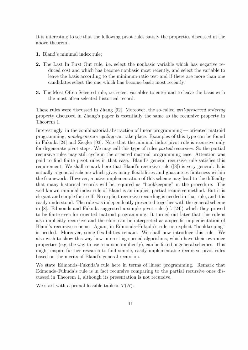
It is interesting to see that the following pivot rules satisfy the properties discussed in theabove theorem.

1. Bland’s minimal index rule;

2. The Last In First Out rule, i.e. select the nonbasic variable which has negative re-duced cost and which has become nonbasic most recently, and select the variable toleave the basis according to the minimum-ratio test and if there are more than onecandidates select the one which has become basic most recently;

3. The Most Often Selected rule, i.e. select variables to enter and to leave the basis withthe most often selected historical record.

These rules were discussed in Zhang [92]. Moreover, the so-called well-preserved orderingproperty discussed in Zhang’s paper is essentially the same as the recursive property inTheorem 1.

Interestingly, in the combinatorial abstraction of linear programming — oriented matroidprogramming, nondegenerate cycling can take place. Examples of this type can be foundin Fukuda [24] and Ziegler [93]. Note that the minimal index pivot rule is recursive onlyfor degenerate pivot steps. We may call this type of rules partial recursive. So the partialrecursive rules may still cycle in the oriented matroid programming case. Attention waspaid to find finite pivot rules in that case. Bland’s general recursive rule satisfies thisrequirement. We shall remark here that Bland’s recursive rule ([8]) is very general. It isactually a general scheme which gives many flexibilities and guarantees finiteness withinthe framework. However, a naive implementation of this scheme may lead to the difficultythat many historical records will be required as “bookkeeping” in the procedure. Thewell known minimal index rule of Bland is an implicit partial recursive method. But it iselegant and simple for itself. No explicit recursive recording is needed in that rule, and it iseasily understood. The rule was independently presented together with the general schemein [8]. Edmonds and Fukuda suggested a simple pivot rule (cf. [24]) which they provedto be finite even for oriented matroid programming. It turned out later that this rule isalso implicitly recursive and therefore can be interpreted as a specific implementation ofBland’s recursive scheme. Again, in Edmonds–Fukuda’s rule no explicit “bookkeeping”is needed. Moreover, some flexibilities remain. We shall now introduce this rule. Wealso wish to show this way how interesting special algorithms, which have their own niceproperties (e.g. the way to use recursion implicitly), can be fitted in general schemes. Thismight inspire further research to find simple, easily implementable recursive pivot rulesbased on the merits of Bland’s general recursion.

We state Edmonds–Fukuda’s rule here in terms of linear programming. Remark thatEdmonds–Fukuda’s rule is in fact recursive comparing to the partial recursive ones dis-cussed in Theorem 1, although its presentation is not recursive.

We start with a primal feasible tableau T (B).

11

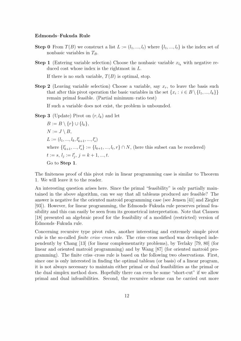
Edmonds–Fukuda Rule

Step 0 From T (B) we construct a list L := (l1, ..., lt) where {l1, ..., lt} is the index set ofnonbasic variables in TB.

Step 1 (Entering variable selection) Choose the nonbasic variable xlk with negative re-duced cost whose index is the rightmost in L.

If there is no such variable, T (B) is optimal, stop.

Step 2 (Leaving variable selection) Choose a variable, say xr, to leave the basis suchthat after this pivot operation the basic variables in the set {xi : i ∈ B \ {l1, ..., lk}}remain primal feasible. (Partial minimum–ratio test)

If such a variable does not exist, the problem is unbounded.

Step 3 (Update) Pivot on (r, lk) and let

B := B \ {r} ∪ {lk},N := J \ B,

L := (l1, ..., lk, l′k+1, ..., l

′s)

where {l′k+1, ..., l′s} := {lk+1, ..., lt, r} ∩ N , (here this subset can be reordered)

t := s, lj := l′j, j = k + 1, ..., t.

Go to Step 1.

The finiteness proof of this pivot rule in linear programming case is similar to Theorem1. We will leave it to the reader.

An interesting question arises here. Since the primal “feasibility” is only partially main-tained in the above algorithm, can we say that all tableaus produced are feasible? Theanswer is negative for the oriented matroid programming case (see Jensen [41] and Ziegler[93]). However, for linear programming, the Edmonds–Fukuda rule preserves primal fea-sibility and this can easily be seen from its geometrical interpretation. Note that Clausen[18] presented an algebraic proof for the feasibility of a modified (restricted) version ofEdmonds–Fukuda rule.

Concerning recursive type pivot rules, another interesting and extremely simple pivotrule is the so-called finite criss–cross rule. The criss–cross method was developed inde-pendently by Chang [13] (for linear complementarity problems), by Terlaky [79, 80] (forlinear and oriented matroid programming) and by Wang [87] (for oriented matroid pro-gramming). The finite criss–cross rule is based on the following two observations. First,since one is only interested in finding the optimal tableau (or basis) of a linear program,it is not always necessary to maintain either primal or dual feasibilities as the primal orthe dual simplex method does. Hopefully there can even be some “short-cut” if we allowprimal and dual infeasibilities. Second, the recursive scheme can be carried out more

12

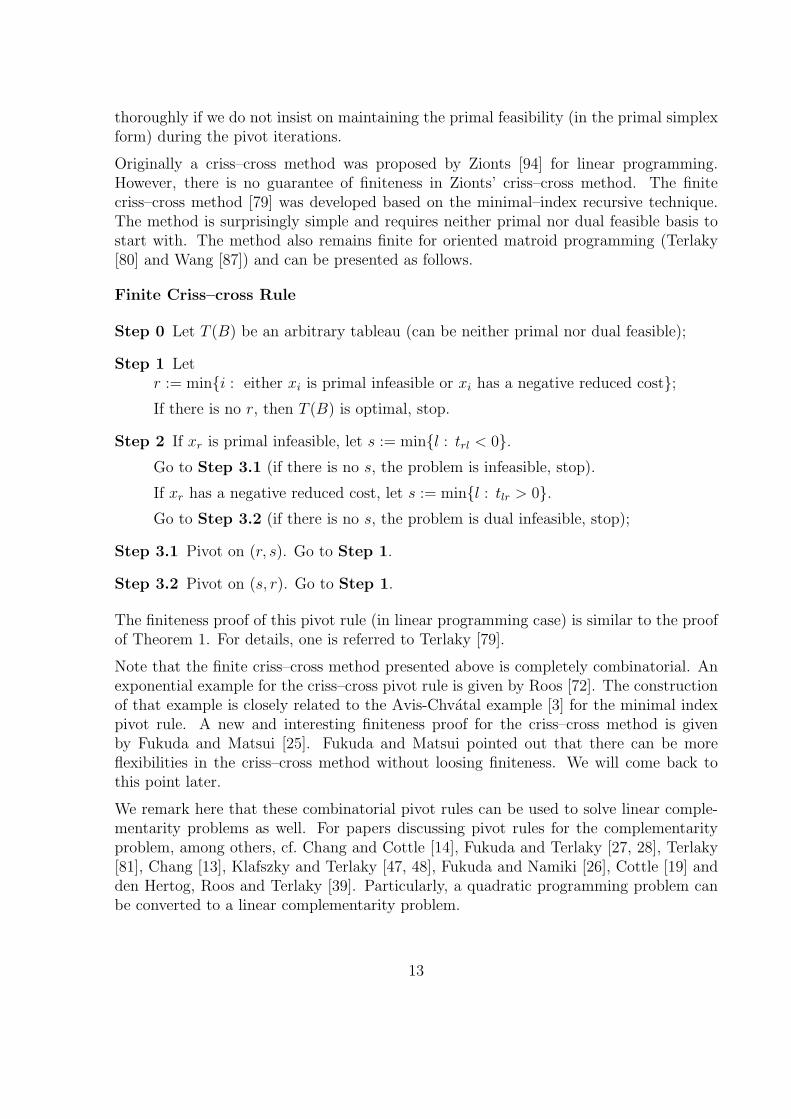
thoroughly if we do not insist on maintaining the primal feasibility (in the primal simplexform) during the pivot iterations.

Originally a criss–cross method was proposed by Zionts [94] for linear programming.However, there is no guarantee of finiteness in Zionts’ criss–cross method. The finitecriss–cross method [79] was developed based on the minimal–index recursive technique.The method is surprisingly simple and requires neither primal nor dual feasible basis tostart with. The method also remains finite for oriented matroid programming (Terlaky[80] and Wang [87]) and can be presented as follows.

Finite Criss–cross Rule

Step 0 Let T (B) be an arbitrary tableau (can be neither primal nor dual feasible);

Step 1 Letr := min{i : either xi is primal infeasible or xi has a negative reduced cost};If there is no r, then T (B) is optimal, stop.

Step 2 If xr is primal infeasible, let s := min{l : trl < 0}.Go to Step 3.1 (if there is no s, the problem is infeasible, stop).

If xr has a negative reduced cost, let s := min{l : tlr > 0}.Go to Step 3.2 (if there is no s, the problem is dual infeasible, stop);

Step 3.1 Pivot on (r, s). Go to Step 1.

Step 3.2 Pivot on (s, r). Go to Step 1.

The finiteness proof of this pivot rule (in linear programming case) is similar to the proofof Theorem 1. For details, one is referred to Terlaky [79].

Note that the finite criss–cross method presented above is completely combinatorial. Anexponential example for the criss–cross pivot rule is given by Roos [72]. The constructionof that example is closely related to the Avis-Chvatal example [3] for the minimal indexpivot rule. A new and interesting finiteness proof for the criss–cross method is givenby Fukuda and Matsui [25]. Fukuda and Matsui pointed out that there can be moreflexibilities in the criss–cross method without loosing finiteness. We will come back tothis point later.

We remark here that these combinatorial pivot rules can be used to solve linear comple-mentarity problems as well. For papers discussing pivot rules for the complementarityproblem, among others, cf. Chang and Cottle [14], Fukuda and Terlaky [27, 28], Terlaky[81], Chang [13], Klafszky and Terlaky [47, 48], Fukuda and Namiki [26], Cottle [19] andden Hertog, Roos and Terlaky [39]. Particularly, a quadratic programming problem canbe converted to a linear complementarity problem.

13

Since minimal index type methods need the indices of variables as an indication of prior-ities of subproblems to be solved recursively, it is profitable to find a “good” ordering ofindices before hand. We can treat such an ordering procedure as pre-conditioning. Pan[66] observed that a facet of a polytope is likely to contain the optimal vertex if the anglebetween its tangent direction and the objective direction is small. Based on this observa-tion, he suggested an ordering of variable indices according to the cosine of the constraints’tangent direction and the objective direction. In fact, Kunzi and Tzschach already tookadvantage of this observation in 1965 when presenting their Duoplex-Algorithm (cf. [53]).

Now we consider again the criss–cross method. We notice that the criss–cross method isa completely recursive procedure, and so it can be linked to the Edmonds–Fukuda rulewhich is also completely recursive. This fact is observed by Fukuda and Matsui [25]. Theyremarked that in order to guarantee the finiteness in the criss–cross rule, only a partialordering of variables is sufficient. At each pivot step we select a variable which is eitherprimal infeasible or has a negative reduced cost according to this partial ordering (fromlow to high), and then we select the pivot element again according to this partial ordering(refer to the criss–cross rule presented above). Denote xt to be the higher one accordingto the partial ordering among entering and leaving variables. In the next iteration, forthose variables higher than xt we keep the same ordering, and for those variables lowerthan xt we let them equal and lower than xt in the new partial ordering. This gives moreflexibility in the criss–cross method and finiteness still can be proved. In fact Fukudaand Matsui [25] and Namiki and Matsui [65] explored more flexibility of the criss–crossmethod.

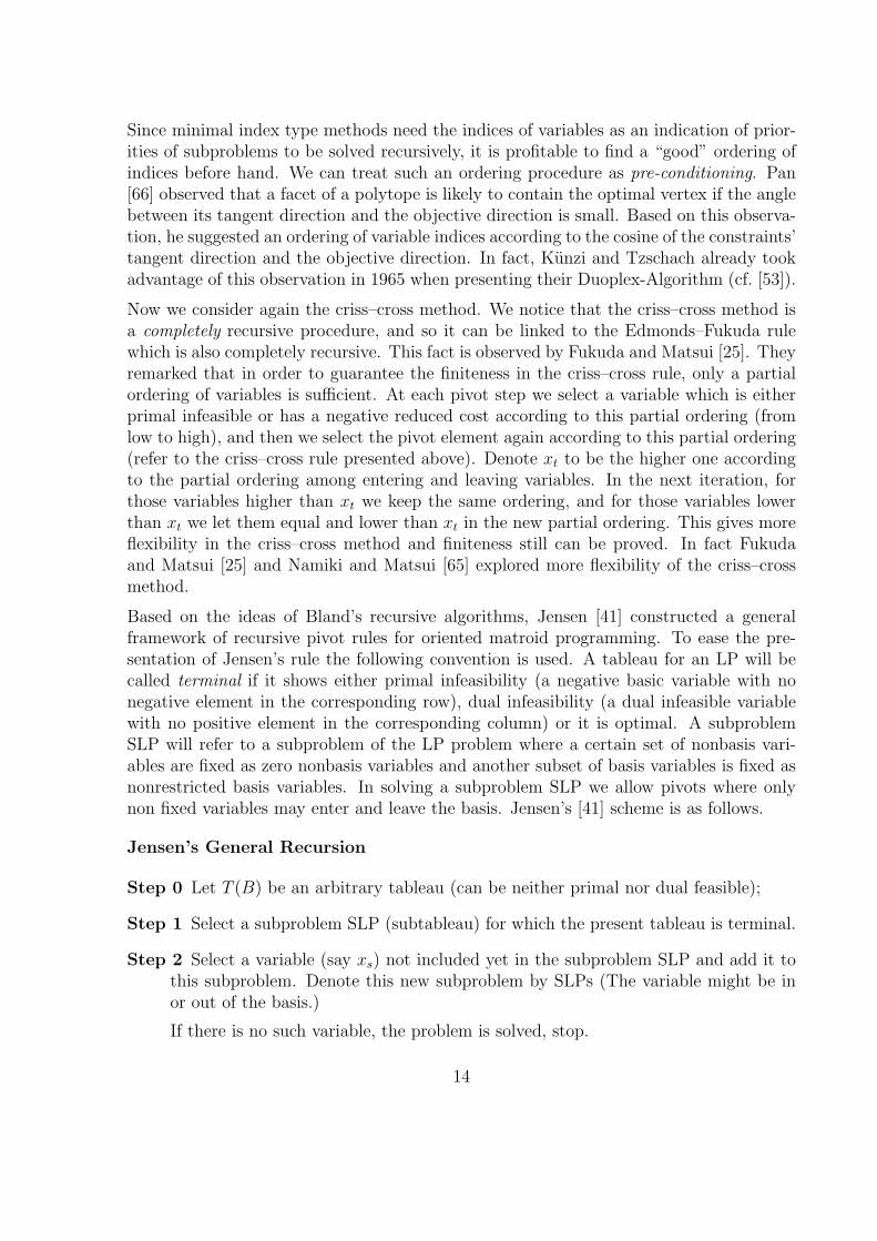
Based on the ideas of Bland’s recursive algorithms, Jensen [41] constructed a generalframework of recursive pivot rules for oriented matroid programming. To ease the pre-sentation of Jensen’s rule the following convention is used. A tableau for an LP will becalled terminal if it shows either primal infeasibility (a negative basic variable with nonegative element in the corresponding row), dual infeasibility (a dual infeasible variablewith no positive element in the corresponding column) or it is optimal. A subproblemSLP will refer to a subproblem of the LP problem where a certain set of nonbasis vari-ables are fixed as zero nonbasis variables and another subset of basis variables is fixed asnonrestricted basis variables. In solving a subproblem SLP we allow pivots where onlynon fixed variables may enter and leave the basis. Jensen’s [41] scheme is as follows.

Jensen’s General Recursion

Step 0 Let T (B) be an arbitrary tableau (can be neither primal nor dual feasible);

Step 1 Select a subproblem SLP (subtableau) for which the present tableau is terminal.

Step 2 Select a variable (say xs) not included yet in the subproblem SLP and add it tothis subproblem. Denote this new subproblem by SLPs (The variable might be inor out of the basis.)

If there is no such variable, the problem is solved, stop.

14

Step 3.1 If the present tableau is terminal for the new subproblem SLPs, then letSLP:=SLPs and Go to Step 2.

Step 3.2 If the tableau is not terminal for SLPs, then make a pivot, change the positionof the new variable xs and fix it in the new position.

Step 4 The subproblem SLP’ obtained so (discarding again xs) has the same numberof variables as it was solved in Step 1. Call recursively this algorithm to solve thisproblem. The terminal tableau for SLP’ is also terminal for SLPs. Let SLP:=SLPsand Go to Step 2.

The finiteness and validity of Jensen’s general recursion can be proved the same way asthe finiteness of the criss–cross method.

Jensen’s work is very general indeed. Many recursive type pivot rules, also the rulesthat we discussed earlier, can be viewed as special variants of Jensen’s general recursivescheme. Therefore the finiteness of these pivot rules can follow from that of Jensen’sscheme. Comparing to Bland’s recursive rule in which the primal feasibility is preserved,Jensen’s rule does not require any primal or dual feasibility. We should observe that therecursive order for the basic and nonbasic variables can be independent. For instance, it ispointed out in [92] that in the primal simplex method for linear programming the minimalindex rule for selecting the entering basis variable together with the last-in-first-out rulefor selecting the leaving basis variable will guarantee no cycling.

Observe also that Jensen’s general recursion is a framework which does not require asimplex procedure. Any method can be applied to find the solution of the subproblems.

Up to now, we have discussed recursive type combinatorial pivot rules for linear program-ming. To conclude this section, we will finally discuss Todd’s finite and feasible pivotrule [83]. So far we can see that most finite pivot rules are of a recursive type. Theserules either do not keep feasibility or may cause nondegenerate cycling in oriented matroidprogramming. Therefore it is theoretically interesting to look for a pivot rule which isfinite and keeps feasibility for oriented matroid programming. To the best knowledgeof the authors, Todd’s rule is the only pivot rule so far proved to be in that category.We notice here that there is a classical technique for preventing cycling in the simplexmethod, known as the lexicographic method. The lexicographic method has an advan-tage that only the selection of the leaving (basis) variable is affected by the method andyet the finiteness is guaranteed. The lexicographic method can also be interpreted as aparametric perturbation method.

The equivalence of the self–dual parametric algorithm and Lemke’s method applied tothe linear complementarity problem defined by the primal and dual LP problem wasproved by Lustig [55]. Todd’s pivot rule is related to the lexicographic Lemke method (orthe parametric perturbation method), and hence using the equivalence mentioned abovea simplex algorithm for LP can be derived. However, it is much more complicated to

15

present this method in a linear programming context. The theoretical meaning mainlyexists in oriented matroid programming.

As Todd’s rule is in fact a lexicographic Lemke method specialized to LP, and the per-turbation is done first in the right hand side and then in the objective (with increasingorder of the perturbation parameter), it gives finally a two phase simplex method. We donot present here the method completely, but only the second phase – without proofs – toillustrate its behaviour. For a complete description we refer to [83, 93].

Todd’s Lexicographic Lemke Rule (Phase II)

Suppose that we are given a feasible tableau T (B).

For a given set of variable indices, say {1, 2, ...,m}, the tableau is called lexico-feasible if

(xi, t(i)m , t

(i)m−1, ..., t

(i)1 )

is lexico-positive (the first nonzero element is positive) for every i ∈ B. It is obvious thatif B = {1, 2, ...,m} then the initial tableau is lexico-feasible.

In the following, at each iteration we always select the entering variable xr such thatzr < 0 and

(t(r)m+1

zr

, ...,t(r)nzr

) = lexico minzj<0

(t(j)m+1

zj

, ...,t(j)nzj

),

where z is the vector of the reduced costs.

For selecting the leaving variable, let the index s of the leaving variable be such that

(xs

trs

,t(s)m

trs

, ...,t(s)1

trs

) = lexico mintri>0

(xi

tri

,t(i)m

tri

, ...,t(i)1

tri

).

It can be seen if l, l + 1, ..., n (l ≥ m + 1) are not in the basis that the variable xk withk ≥ l is selected to enter the basis only if zj ≥ 0 for j ∈ {1, 2, ...,m,m + 1, ..., l − 1}.Similar properties hold for variables leaving the basis. This monotonicity guarantees nocycling.

The practical behavior of this method is similar to Bland’s minimal index rule. To imple-ment Todd’s rule is more complicated, but not much more expensive. A big drawback, asin general with lexicographic rules, is deciding when two entries are equal within roundoff errors.

It is still interesting to give an easy and clear proof of the correctness of Todd’s rule. Also,it is unknown if there are some other alternative simplex pivot rules which guaranteefiniteness in the context of oriented matroid programming.

This concludes this section. In the following section, we will discuss some pivot rulesespecially for linear programming. They may not guarantee anti-cycling if there is nospecial treatment. Attention is mainly paid to the numerical structure of the problem.To derive other finite variants, note that the methods discussed in the next section canbe combined with (partial) recursive rules of this section and with the lexicographic rule.

16

3 Pivot Rules Related to Parametric Programming

The algorithms discussed in this section are closely related to parametric programming,more precisely to the shadow vertex algorithm [11, 34, 61] and to Dantzig’s self–dualparametric simplex algorithm [20].

As was mentioned in the previous section, the self–dual parametric algorithm is equivalentto Lemke’s method applied to the linear complementarity problem defined by the primaland dual LP problem. For details see Lustig [55]. It is also easy to see that the shadowvertex algorithm can be interpreted as a special case of the self–dual parametric simplexalgorithm and so only the shadow vertex algorithm will be discussed here. Using the abovementioned correspondence the reader can easily derive the connection between the newalgorithms and the self–dual parametric algorithm (and the relation to Lemke’s method).

Before presenting the algorithms, note that a variable will be called a driving variable ifit plays a special role in the pivot selection, namely the leaving (or entering) variable issubsequentially determined by using this column (or row).

Anstreicher and Terlaky [1] presented the monotonic build-up simplex algorithm (MBU).We start our discussion by presenting MBU. This is due to the fact that, as will be shown,the Exterior Point Simplex Algorithm [68, 69] (EPSA), the shadow vertex algorithm andMagnanti and Orlin’s [56] parametric programming algorithm can be interpreted as specialimplementations of MBU.

There are two interesting properties of MBU. On one hand there are two ratio tests inevery pivot step — both the leaving and entering variables are selected by performing aratio test. Dual feasibility (for the variables that are already dual feasible) is preservedduring the algorithm – due to the second ratio test – while primal feasibility is temporarilylost, but recovered time to time. On the other hand, MBU is in fact a simplex method,since a primal feasible basis is associated with each basis of MBU.

Monotonic Build Up Simplex Algorithm MBU

As in the primal simplex method, let us assume that a primal feasible basic solution isavailable. The pivot rule is as follows.

MBU - The Pivot Rule

Step 0 Let J+ = {j : zj ≥ 0}, J− = J \ J+ = {j : zj < 0}.Step 1 Let k ∈ J− be an arbitrary index. (Variable xk will be referred as the driving

variable.)If J− = ∅, then an optimal solution is found, stop.

Step 2 Leaving variable selectionLet r = argmin{ xi

tik: tik > 0}. (xr is the leaving variable.)

If there is no r, then the problem is unbounded, stop.

17

Step 3 Entering variable selectionLet s = argmin{− zj

trj: trj < 0, j ∈ J+}. If there is no s, then let s = k.

Let θ1 = − zs

trsand θ2 = − zk

trk.

Step 3a If θ1 < θ2, then make a pivot on (r, s), xr enters the basis. Let J+ = {j : zj ≥ 0}.The driving variable is not changed. Go to Step 2.

Step 3b If θ1 ≥ θ2, then make a pivot on (r, k), xk enters the basis. Let J+ = {j : zj ≥ 0}.Go to Step 1.

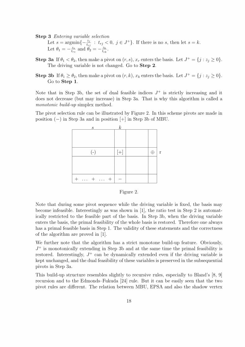
Note that in Step 3b, the set of dual feasible indices J+ is strictly increasing and itdoes not decrease (but may increase) in Step 3a. That is why this algorithm is called amonotonic build-up simplex method.

The pivot selection rule can be illustrated by Figure 2. In this scheme pivots are made inposition (−) in Step 3a and in position [+] in Step 3b of MBU.

s k

(-) [+] ⊕ r

+ . . . + . . . + −

Figure 2.

Note that during some pivot sequence while the driving variable is fixed, the basis maybecome infeasible. Interestingly as was shown in [1], the ratio test in Step 2 is automat-ically restricted to the feasible part of the basis. In Step 3b, when the driving variableenters the basis, the primal feasibility of the whole basis is restored. Therefore one alwayshas a primal feasible basis in Step 1. The validity of these statements and the correctnessof the algorithm are proved in [1].

We further note that the algorithm has a strict monotone build-up feature. Obviously,J+ is monotonically extending in Step 3b and at the same time the primal feasibility isrestored. Interestingly, J+ can be dynamically extended even if the driving variable iskept unchanged, and the dual feasibility of these variables is preserved in the subsequentialpivots in Step 3a.

This build-up structure resembles slightly to recursive rules, especially to Bland’s [8, 9]recursion and to the Edmonds–Fukuda [24] rule. But it can be easily seen that the twopivot rules are different. The relation between MBU, EPSA and also the shadow vertex

18

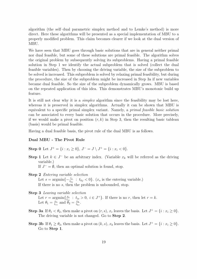
algorithm (the self–dual parametric simplex method and to Lemke’s method) is moredirect. Here these algorithms will be presented as a special implementation of MBU to aproperly modified problem. This claim becomes clearer if we look at the dual version ofMBU.

We have seen that MBU goes through basic solutions that are in general neither primalnor dual feasible, but some of these solutions are primal feasible. The algorithm solvesthe original problem by subsequently solving its subproblems. Having a primal feasiblesolution in Step 1 we identify the actual subproblem that is solved (collect the dualfeasible variables). Then by choosing the driving variable, the size of the subproblem tobe solved is increased. This subproblem is solved by relaxing primal feasibility, but duringthe procedure, the size of the subproblem might be increased in Step 3a if new variablesbecame dual feasible. So the size of the subproblem dynamically grows. MBU is basedon the repeated application of this idea. This demonstrates MBU’s monotonic build upfeature.

It is still not clear why it is a simplex algorithm since the feasibility may be lost here,whereas it is preserved in simplex algorithms. Actually it can be shown that MBU isequivalent to a specific primal simplex variant. Namely, a primal feasible basic solutioncan be associated to every basic solution that occurs in the procedure. More precisely,if we would make a pivot on position (r, k) in Step 3, then the resulting basic tableau(basis) would be primal feasible.

Having a dual feasible basis, the pivot rule of the dual MBU is as follows.

Dual MBU - The Pivot Rule

Step 0 Let J+ = {i : xi ≥ 0}, J− = J \ J+ = {i : xi < 0}.Step 1 Let k ∈ J− be an arbitrary index. (Variable xk will be referred as the driving

variable.)If J− = ∅, then an optimal solution is found, stop.

Step 2 Entering variable selectionLet s = argmin{− zj

tkj: tkj < 0}. (xs is the entering variable.)

If there is no s, then the problem is unbounded, stop.

Step 3 Leaving variable selectionLet r = argmin{ xi

tis: tis > 0, i ∈ J+}. If there is no r, then let r = k.

Let θ1 = xr

trsand θ2 = xk

tks.

Step 3a If θ1 < θ2, then make a pivot on (r, s), xr leaves the basis. Let J+ = {i : xi ≥ 0}.The driving variable is not changed. Go to Step 2.

Step 3b If θ1 ≥ θ2, then make a pivot on (k, s), xk leaves the basis. Let J+ = {i : xi ≥ 0}.Go to Step 1.

19

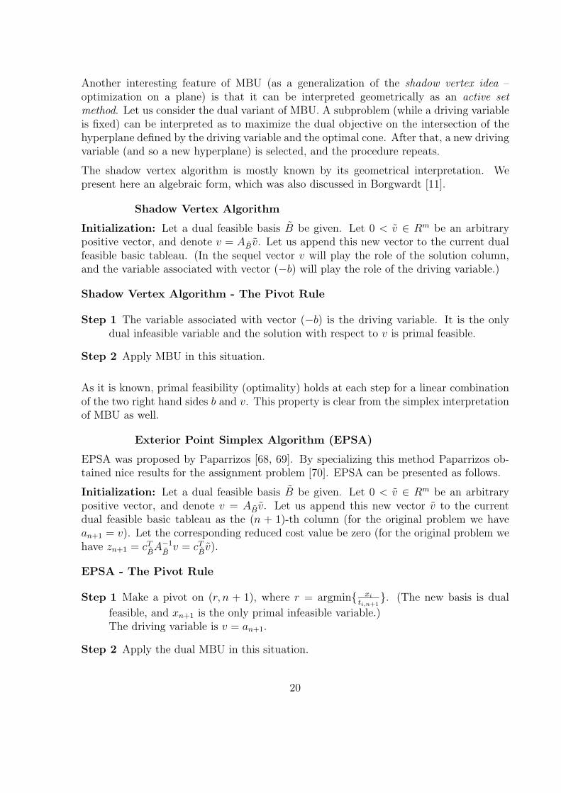
Another interesting feature of MBU (as a generalization of the shadow vertex idea –optimization on a plane) is that it can be interpreted geometrically as an active setmethod. Let us consider the dual variant of MBU. A subproblem (while a driving variableis fixed) can be interpreted as to maximize the dual objective on the intersection of thehyperplane defined by the driving variable and the optimal cone. After that, a new drivingvariable (and so a new hyperplane) is selected, and the procedure repeats.

The shadow vertex algorithm is mostly known by its geometrical interpretation. Wepresent here an algebraic form, which was also discussed in Borgwardt [11].

Shadow Vertex Algorithm

Initialization: Let a dual feasible basis B be given. Let 0 < v ∈ Rm be an arbitrarypositive vector, and denote v = AB v. Let us append this new vector to the current dualfeasible basic tableau. (In the sequel vector v will play the role of the solution column,and the variable associated with vector (−b) will play the role of the driving variable.)

Shadow Vertex Algorithm - The Pivot Rule

Step 1 The variable associated with vector (−b) is the driving variable. It is the onlydual infeasible variable and the solution with respect to v is primal feasible.

Step 2 Apply MBU in this situation.

As it is known, primal feasibility (optimality) holds at each step for a linear combinationof the two right hand sides b and v. This property is clear from the simplex interpretationof MBU as well.

Exterior Point Simplex Algorithm (EPSA)

EPSA was proposed by Paparrizos [68, 69]. By specializing this method Paparrizos ob-tained nice results for the assignment problem [70]. EPSA can be presented as follows.

Initialization: Let a dual feasible basis B be given. Let 0 < v ∈ Rm be an arbitrarypositive vector, and denote v = AB v. Let us append this new vector v to the currentdual feasible basic tableau as the (n + 1)-th column (for the original problem we havean+1 = v). Let the corresponding reduced cost value be zero (for the original problem wehave zn+1 = cT

BA−1

Bv = cT

Bv).

EPSA - The Pivot Rule

Step 1 Make a pivot on (r, n + 1), where r = argmin{ xi

ti,n+1}. (The new basis is dual

feasible, and xn+1 is the only primal infeasible variable.)The driving variable is v = an+1.

Step 2 Apply the dual MBU in this situation.

20

It is obvious that, after Step 1 we have an almost optimal basis except one primal infeasiblevariable.

EPSA and the shadow vertex algorithm have the common idea to introduce an auxiliaryvector to force primal feasibility. The main difference is that an additional pivot is per-formed in EPSA. (A pivot in the v−row of the tableau.) Based on this observation it iseasy to see that EPSA and the shadow vertex algorithm are also closely related.

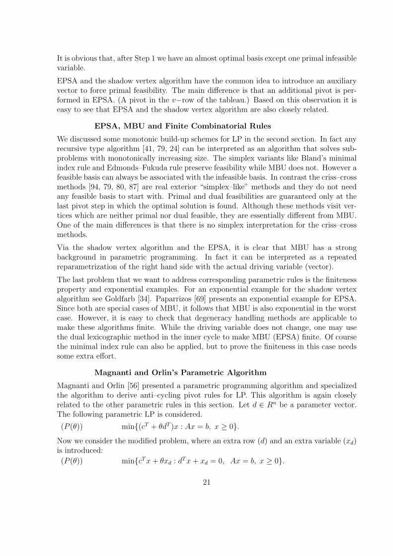
EPSA, MBU and Finite Combinatorial Rules

We discussed some monotonic build-up schemes for LP in the second section. In fact anyrecursive type algorithm [41, 79, 24] can be interpreted as an algorithm that solves sub-problems with monotonically increasing size. The simplex variants like Bland’s minimalindex rule and Edmonds–Fukuda rule preserve feasibility while MBU does not. However afeasible basis can always be associated with the infeasible basis. In contrast the criss–crossmethods [94, 79, 80, 87] are real exterior “simplex–like” methods and they do not needany feasible basis to start with. Primal and dual feasibilities are guaranteed only at thelast pivot step in which the optimal solution is found. Although these methods visit ver-tices which are neither primal nor dual feasible, they are essentially different from MBU.One of the main differences is that there is no simplex interpretation for the criss–crossmethods.

Via the shadow vertex algorithm and the EPSA, it is clear that MBU has a strongbackground in parametric programming. In fact it can be interpreted as a repeatedreparametrization of the right hand side with the actual driving variable (vector).

The last problem that we want to address corresponding parametric rules is the finitenessproperty and exponential examples. For an exponential example for the shadow vertexalgorithm see Goldfarb [34]. Paparrizos [69] presents an exponential example for EPSA.Since both are special cases of MBU, it follows that MBU is also exponential in the worstcase. However, it is easy to check that degeneracy handling methods are applicable tomake these algorithms finite. While the driving variable does not change, one may usethe dual lexicographic method in the inner cycle to make MBU (EPSA) finite. Of coursethe minimal index rule can also be applied, but to prove the finiteness in this case needssome extra effort.

Magnanti and Orlin’s Parametric Algorithm

Magnanti and Orlin [56] presented a parametric programming algorithm and specializedthe algorithm to derive anti–cycling pivot rules for LP. This algorithm is again closelyrelated to the other parametric rules in this section. Let d ∈ Rn be a parameter vector.The following parametric LP is considered.

(P (θ)) min{(cT + θdT )x : Ax = b, x ≥ 0}.Now we consider the modified problem, where an extra row (d) and an extra variable (xd)is introduced:

(P (θ)) min{cT x + θxd : dT x + xd = 0, Ax = b, x ≥ 0}.

21

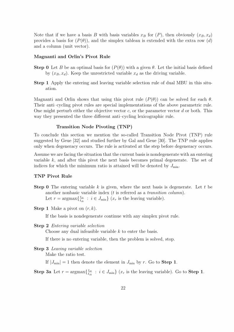
Note that if we have a basis B with basis variables xB for (P ), then obviously (xB, xd)provides a basis for (P (θ)), and the simplex tableau is extended with the extra row (d)and a column (unit vector).

Magnanti and Orlin’s Pivot Rule

Step 0 Let B be an optimal basis for (P (θ)) with a given θ. Let the initial basis definedby (xB, xd). Keep the unrestricted variable xd as the driving variable.

Step 1 Apply the entering and leaving variable selection rule of dual MBU in this situ-ation.

Magnanti and Orlin shows that using this pivot rule (P (θ)) can be solved for each θ.Their anti–cycling pivot rules are special implementations of the above parametric rule.One might perturb either the objective vector c, or the parameter vector d or both. Thisway they presented the three different anti–cycling lexicographic rule.

Transition Node Pivoting (TNP)

To conclude this section we mention the so-called Transition Node Pivot (TNP) rulesuggested by Geue [32] and studied further by Gal and Geue [30]. The TNP rule appliesonly when degeneracy occurs. The rule is activated at the step before degeneracy occurs.

Assume we are facing the situation that the current basis is nondegenerate with an enteringvariable k, and after this pivot the next basis becomes primal degenerate. The set ofindices for which the minimum ratio is attained will be denoted by Jmin.

TNP Pivot Rule

Step 0 The entering variable k is given, where the next basis is degenerate. Let t beanother nonbasic variable index (t is referred as a transition column).Let r = argmax{ tit

tik: i ∈ Jmin} (xr is the leaving variable).

Step 1 Make a pivot on (r, k).

If the basis is nondegenerate continue with any simplex pivot rule.

Step 2 Entering variable selectionChoose any dual infeasible variable k to enter the basis.

If there is no entering variable, then the problem is solved, stop.

Step 3 Leaving variable selectionMake the ratio test.

If |Jmin| = 1 then denote the element in Jmin by r. Go to Step 1.

Step 3a Let r = argmax{ tittik

: i ∈ Jmin} (xr is the leaving variable). Go to Step 1.

22

Similarly as with the previous parametric rules the TNP rule can be combined with theminimal index or lexicographic rule to guarantee finiteness of the procedure. A “pertur-bation” column as the transition column can be introduced as with the lexicographic rule.Then the reduced cost of this extra column strictly increases, and hence cycling becomesimpossible.

4 Pivot Rules Related to Interior Point Methods

In this section we will discuss some recent pivot rules for the simplex method whichare in one way or another related to interior point methods. Since Karmarkar [43] firstproposed an interior method which solves linear programming problems in polynomialtime and this method is reported to perform superior to the simplex method for largescale problems, there have been a large number of research papers devoted to that topic.Interior point methods allow the iterative points to go inside the polytope and they arebelieved to be able to use more global information and therefore to avoid “myopia” of thesimplex method. Although it is still unclear that we may succeed in finding a polynomialsimplex algorithm by using interior point type methodology, we think it is definitely anew field deserving further investigation. In this section mainly three pivot rules will bediscussed. They are: Todd’s rule [84] which was obtained as a limit of a projective interiorpoint method, the minimal volume simplex rule of Roos [71] and the dual interior primalsimplex method of Tamura, Takehara, Fukuda, Fujishige and Kojima [78].

Todd’s Dantzig–Wolfe Like Pivot Rule

The pivot rule proposed by Todd [84] is closely related to the pivot rules presented byKlotz [51]. These rules are based on the reduced cost scaling as it was earlier used byHarris [37] in the DEVEX code and also studied by Kalan [42]. Reduced cost scaling withvarious scaling methods and their effect on the numerical performance of the simplexalgorithm is extensively studied by Klotz [51]. Todd’s pivot rule is based on a variant ofKarmarkar’s interior point method (cf. Todd [84]). The method is described as follows.

We consider the linear programming in the following form

min cT x

s.t. Ax = 0

gT x = 1

x ≥ 0,

where g is a certain vector.Let xk be an interior point in the feasible region of the above problem. Let X = Xk :=diag(xk) denote the diagonal matrix with diagonal entries the coordinates of xk. Define

23

the oblique projection matrix

P = Pk := I − X2AT (AX2AT )−1A.

It is easy to see that AP = 0 and P 2 = P .

Let the oblique projection of c and g be given as

c := P T c and g := P T g.

The relaxed problem is defined by

(RP) min cT x

s.t. gT x = 1

x ≥ 0.

Note that (RP) is a continuous knapsack problem and it can be solved easily. If (RP)has an optimal solution w, let w := Pw. If (RP) is unbounded with an unbounded raydirection t, let t := Pt. In the first case, let xk+1 := (1 − λk)x

k + λkw, λk ∈ (0, 1]. Inthe second case, let xk+1 := xk + μk t, μk > 0. With proper choice of λk or μk, andusing Karmarkar’s potential function, Todd [84] proved that this method has the sameconvergence property as Karmarkar’s method.

Now, if xk is a nondegenerate basic feasible solution with basis B, a similar procedurecan be applied. This results in the following pivot rule.

Todd’s Projective Pivot Rule

Step 1 Let B be a primal feasible basis and suppose P solves ATBP = cB and σ solves

ATBσ = X−1

B e where XB is the diagonal matrix with diagonal entries the values ofthe basic variables and e is the vector with each component equal to 1. For eachj �∈ B, compute the reduced cost zj := cj − P T aj and gj := σT aj.

Step 2 If there is an r with zr < 0 and gr = 0, select it as the entering basis variableindex.

Otherwise, select r = arg max{ zj

gj: zj < 0, gj < 0}.

Else, select r = argmin{ zj

gj: zj < 0, gj > 0}.

If none of these applies, the current basis is optimal, stop.

Step 3 Select the leaving variable according to the usual minimum ratio test. If noleaving variable is found, the problem is unbounded, otherwise go to Step 1.

24

Reduced cost scaling is used in Todd’s pivot rule. More analyses can be found in Todd’spaper [84]. We note here that in case of degeneracy additional rules need to be adaptedto prevent cycling.

Minimal Volume Simplex Pivot Rule

The minimal volume simplex pivot rule is suggested in an unpublished paper of Roos[71]. In Roos’ paper, the primal problem (P ) is considered. As in Karmarkar’s approach,he assumes that the optimal value is known to be zero (this assumption is standardin the analysis of projective methods). Moreover, all basic solutions are assumed to benondegenerate. For a given basis B, let AB be the submatrix of A and cB be the subvectorof c corresponding to the index set (basis) B. Now, consider a cone CB in Rm associatedwith the basis B as follows:

CB := {y ∈ Rm : ATBy ≤ cB}.

If the rows of A−1B are given by y1, y2, ..., ym, then it can be shown that

CB = {yB −m∑

i=1

λiyi : λi ≥ 0, i = 1, 2, ...,m},

where yTB := cT

BA−1B .

Moreover, the vectors yi, i = 1, 2, ...,m, are the rays of the cone CB. By the definition ofthe tableau, it is obvious that tij = yT

i aj, i = 1, 2, ...,m, j = 1, 2, ..., n.

The problem max{yT b : y ∈ CB} is bounded from above if and only if yTi b ≥ 0 for

i = 1, 2, ...,m, and this corresponds to the feasibility of the basis B. Suppose the feasiblebasis B is not optimal. Remember that the optimal value was assumed to be zero,this means that yT

Bb > 0. Therefore the intersection of the cone CB and the half space{y : yT b ≥ 0} forms a nontrivial simplex. We denote this simplex by SB. It is shown inRoos [71] that the volume of SB can be computed as

vol(SB) =1

n!

(cT x)n

∏x

1

| det AB | ,

where Πx denotes the product of positive entries of x. The minimal volume pivot ruleof Roos seeks for the next feasible basis with the minimal volume of such simplex. Notehere that the simplex corresponding to the optimal basis has zero volume.

To calculate the volume of this simplex does not need much effort. If the pivot elementis denoted by trs, then it follows that | det AB′ |= trs | det AB | with B′ the next feasiblebasis. Hence Roos’ pivot rule looks for the entering variable index r with zr < 0 and thefeasible pivot element trs such that

1

trs

(cT x′)n

∏x′

25

is minimal, where x′ denotes the basic feasible solution corresponding to the next feasiblebasis B′.

Observe that this formula strongly resembles Karmarkar’s potential function. However, itis still unclear at this stage how to cope with the degenerate case. Also, more propertiesof this method need to be investigated. In formal presentation, Roos’ pivot rule is asfollows.

Roos’ Pivot Rule

Step 1 For an LP problem in the primal form having optimal value zero, let B be afeasible basis. Let yT := cT

BAB and the reduced cost vector zT := cT − yT A.

Step 2 For all possible pivot on position (r, s) with zr < 0 preserving primal feasibility,compute

1

trs

(cT x′)n

∏x′

where x′ is the next basic feasible solution, and select the pair (r, s) with the minimalvalue. Pivot on that position and go to Step 1.

Concerning Roos’ unpublished paper [71] we note that he also presented another pivotrule, the so-called maximum distance pivot rule. Here the variable is selected to enterthe basis for which the corresponding hyperplane (in the dual formulation) is the farthestfrom the present vertex.

Dual Interior Primal Simplex Method (DIPS)

Finally in this section we will introduce the socalled Dual Interior Primal Simplex (DIPS)method developed by Tamura, Takehara, Fukuda, Fujishige and Kojima [78]. This methodis also referred sometimes as Stationary Ball Method. DIPS is a modification of thegravitational method of Chang and Murty [64] and Murty [62]. The gravitational methodcan be explained as follows.

We consider the dual problem (D) : max{bT y : AT y ≤ c}. Suppose the interior of{y : AT y ≤ c} is nonempty, then we can place a ball with certain radius r inside thatregion. Now, suppose the objective direction b is vertical, the ball will then fall down bythe gravitational force until it touches some boundary of that region and rolls down whileminimizing its potential energy. If we then reduce the radius of the ball subsequentially tozero, it will fall and roll down until it reaches the “bottom” of the feasible region (optimalpoint).

If an initial ball in a stationary position is known, and the radius of the ball is reduceddiscretely to zero, it can be shown under the nondegeneracy assumption, that the trajec-tory of the centers of the ball is a piece-wise linear locus. The gravitational method ofChang and Murty is to follow this central trajectory until certain precision requirementsare satisfied. Their method is finite.

26

The DIPS method is based on a similar idea. An essential observation (Chang and Murty[15], Murty [64], and Tamura et al. [78]) is that a subset of constraints touched by a ballin its stationary position (after falling down) forms a feasible basis for the primal problem(P ). Moreover, two adjacent break points in the central trajectory result in two differentbut adjacent bases of the primal problem. For detailed proofs, one refers to Tamura etal. [78]. This trajectory is related to the “inverse barrier path” and is discussed by DenHertog, Roos and Terlaky [40].

To derive a pivot rule some additional assumptions were needed. In the original paper itwas assumed that ||aj|| = 1 for all j and the LP problem is dual nondegenerate. Note thatthe first assumption is not restrictive since it can be easily obtained by scaling; moreover,the resulted pivot rule can be presented without the second assumption as will be seenlater.

Let yi, i = 1, 2, ..., denote the break points of the piecewise linear central trajectory andBi the feasible basis corresponding to the dual constraints reached by the ball with centeryi and with the maximum radius ri of that position. Furthermore, if xi denotes the basicfeasible solution corresponding to the basis Bi, i = 1, 2, ..., it is shown by Tamura et al.that

cT xi+1 ≤ cT xi, i = 1, 2, ...

bT yi+1 ≥ bT yi, i = 1, 2, ...

andlimi→∞

cT xi = limi→∞

bT yi.

This explains the name of the method (Dual Interior Primal Simplex).

More specifically, the rule for selecting the entering basis variable in the primal simplexversion can be stated explicitly as follows2.

Dual Interior Pivot Rule

Step 1 For a primal feasible tableau T (B), where B corresponds to indices of dual con-straints touched by the ball with center y and radius r in the dual space, if there isa nonbasic index k such that aT

k y − ck = −‖ak‖r (i.e. the hyperplane correspondingto index k also touches the ball) then we set the entering index s to be the minimalindex among such nonbasic variables; otherwise select

s = argminck−aTk

z<0{(aT

k y − ck + ‖ak‖r) + (ck − aTk w)

aTk y − ck + ‖ak‖r }

where wT := cTBA−1

B , ak denotes the kth column of A, ck the kth coordinate of c(therefore ck − aT

k w is the reduced cost of xk).

Step 2 Select the leaving basis variable according to the usual simplex ratio test. Updatethe basis B and go to Step 1.

2This formulation is given to the authors by Professor Tamura [77].

27

The DIPS method is reported to have similar numerical behavior as the maximum decreasepivot rule, whereas the complexity to perform each pivot is much less. Also, relationsbetween the DIPS method and the parametric programming technique were discussed in[78]. This concludes the DIPS method and this section.

There are many interesting results related to pivot rules, as well as many open questions.In the next section, we will conclude the paper with some remarks.

5 Miscellaneous Remarks

Although interior point methods have been most intensively studied in the last years,several pivot rules were developed for linear programming. We have surveyed three classesof pivot rules – combinatorial, parametric type and those derived from interior pointmethods.

An interesting (and efficient) application of the minimal index rule and the criss–crossmethod is presented by Avis and Fukuda [4]. By reversing these rules an algorithm isderived that enumerates all the feasible bases (vertices of a polyhedra) and all the baseswithout extra storage requirement.

Concerning combinatorial pivot rules note that there are a great number of pivot rulesdeveloped for special classes of network optimization. Most of them were never studiedor generalized for general linear programming. To discuss these rules is beyond the scopeof the present paper. We also note that it is interesting to find a simple finiteness prooffor Todd’s simplex pivot rule for oriented matroid programming, or to find some otherpivot rules belonging to this category.

Interestingly, only simplex methods based on parametric programming – the shadow ver-tex algorithm and Lemke’s method – are proved to be polynomial in the expected numberof pivot steps [11, 85]. It is still unknown if the other rules have this property as well.To the best knowledge of the authors only one attempt was made to examine the averagenumber of steps of combinatorial pivot rules [26].

In the extensive literature of interior point methods one can find some papers discussingthe relation between interior point methods and the simplex methods. Among them,there are papers by Chiu and Ye [16] and by Stone and Tovey [76]. In the last paper thesimplex method and interior point methods were presented as iteratively reweighted leastsquares methods.

Sehti and Thompson [75] proposed the Pivot and Probe method where the simplex methodwas combined with a build–up structure. This algorithm appeared before the theory ofinterior point methods became the central area for research in linear programming.

Another recent trend to improve the efficiency of LP algorithms is to combine interiorpoint algorithms with the simplex method. In this approach some interior point method isfirst applied to generate a sufficiently good interior solution, then the algorithm switches

28

to the simplex method to find an optimal basis. This type of methods are discussed in[52, 57, 58, 7, 90].

Although to discuss “practical pivot rules” and implementation strategies is beyond thescope of this paper we mention here some recent papers discussing practical problemsand state of the art implementations. The paper of Forrest and Tomlin [23] discussesthe implementation of the simplex method in IBM’s Optimization Subroutine Library.The papers of Bixby [5, 6] discuss the implementational issues of the CPLEX package.Practical degeneracy handling strategies are presented and tested in [12, 17, 35, 33, 38, 73].Most of the efficient packages [6, 23] utilize the advantages of DEVEX rules (which arebased on reduced cost scaling) [37, 42, 51] and a composite objective function [6, 23, 21](which is a linear combination of the original objective function and a linear functionmeasuring infeasibility).

The steepest edge simplex algorithm also shows practical efficiency as it is presented in[35]. Boyd [11] presents some modifications of the steepest edge algorithm for resolvingdegeneracy in combinatorial linear programming problems. He proves that the steepestascent algorithm is finite. However, the solution of a quadratic programming problem isneeded to find the steepest ascent direction.

Towards degeneracy in linear programming and some other related problems, there is arelatively new approach called theory of degeneracy graphs studied by Gal et al. [29].In that theory, a degenerate vertex is associated with a graph. Each node of the graphrepresents a basis corresponding to the vertex. An edge between two nodes on the graphimplies that a pivot step can be performed to move from one basis to the other. To studythis graph will certainly give insight about the structure of the degenerate vertex.

To conclude the paper we note that the hardest and long standing open problems in thetheory of linear programming are still concerned with pivot methods. Those include thed–step conjecture [50] and the question whether there exists a polynomial pivot rule ornot. For the last problem Zadeh’s rule [91] might be a candidate. At least it is still notproved to be exponential in the worst case.

Acknowledgements

The authors are grateful to the anonymous referees and Hans Frenk for the constructivecomments on the first version of the paper.

29

References

[1] K.M. Anstreicher and T. Terlaky, A Monotonic Build Up Simplex Algorithm, Re-port 91–82, Faculty of Technical Mathematics and Informatics, Delft University ofTechnology, The Netherlands (1990).

[2] I. Adler and N. Megiddo, A Simplex Algorithm Whose Average Number of Steps isBounded Between Two Quadratic Functions of the Smaller Dimension, Journal ofthe Association of Computing Machinery 32(1985)891–895.

[3] D. Avis and V. Chvatal, Notes on Bland’s Rule, Mathematical Programming Study8(1978)24–34.

[4] D. Avis and K. Fukuda, A Pivoting Algorithm for Convex Hulls and Vertex Enu-meration of Arrangements and Polyhedra, Research Report B-237, Department ofInformation Sciences, Tokyo Institute of Technology, Tokyo, Japan (1991).

[5] R.E. Bixby, Implementing the Simplex Method: The Initial Basis, Report TR90–32,Department of Mathematical Sciences, Rice University, Texas, USA (1991).

[6] R.E. Bixby, The Simplex Method: It Keeps Getting Better, Lecture at the 14th Inter-national Symposium on Mathematical Programming, Amsterdam, The Netherlands(1991).

[7] R.E. Bixby, J.W. Gregory, I.J. Lustig, R.E. Marsten and D.F. Shanno, Very Large–Scale Linear Programming: A Case Study in Combining Interior Point and SimplexMethods, Report, Department of Mathematical Sciences, Rice University, Texas,USA (1991).

[8] R.G. Bland, New Finite Pivoting Rules for the Simplex Method, Mathematics ofOperations Research 2(1977)103–107.

[9] R.G. Bland, A Combinatorial Abstraction of Linear Programming, Journal of Com-binatorial Theory (Ser. B) 23(1977)33–57.

[10] K.H. Borgwardt, The Simplex Method: A Probabilistic Analysis, Algorithms andCombinatorics, Vol. 1. (Springer Verlag, 1987).

[11] E.A. Boyd, Resolving Degeneracy in Combinatorial Linear Programs: Steepest Edge,Steepest Ascent and Closest Ascent, Report, Department of Mathematical Sciences,Rice University, Texas, USA (1992).

[12] N. Cameron, Stationarity in the Simplex Method, Journal of the Australian Mathe-matical Society 43(1987)137–142.

[13] Y.Y. Chang, Least Index Resolution of Degeneracy in Linear Complementarity Prob-lems, Technical Report 79–14, Department of Operations Research, Stanford Univer-sity, Stanford, California, USA (1979).

30

[14] Y.Y. Chang and R.W. Cottle, Least Index Resolution of Degeneracy in QuadraticProgramming, Mathematical Programming 18(1980)127–137.

[15] S.Y. Chang and K.G. Murty, The Steepest Descent Gravitational Method for LinearProgramming, Discrete and Applied Mathematics, 25(1989)211–239.

[16] S.S. Chiu and Y. Ye, Simplex Method and Karmarkar’s Algorithm: A UnifyingStructure, Technical Report, Engineering Economic Systems Department, StanfordUniversity, Stanford, California, USA (1985).

[17] M. Cirina, Remarks on a Recent Simplex Pivoting Rule, Methods of OperationsResearch 49(1985)187–199.

[18] J. Clausen, A Note on Edmonds–Fukuda Pivoting Rule for the Simplex Method,European Journal of Operations Research 29(1987)378–383.

[19] R.W. Cottle, The Principal Pivoting Method Revisited, Technical Report SOL 89–3,Stanford University, Stanford, California, USA (1989).

[20] G.B. Dantzig, Linear Programming and Extensions (Princeton University Press,Princeton N.J., 1963)

[21] H.A. Eiselt and C.-L. Sandblom, External Pivoting in the Simplex Algorithm, Sta-tistica Neerlandica 39(1985)327–341.

[22] J. Folkman and J. Lawrence, Oriented Matroids, Journal of Combinatorial Theory(Ser. B) 25(1978)199–236.

[23] J.J.H. Forrest and J.A. Tomlin, Implementing the Simplex Method for the Optimiza-tion Subrutin Library, IBM Systems Journal 31(1992)11–25.

[24] K. Fukuda, Oriented Matroid Programming, Ph.D. Thesis, Waterloo University, Wa-terloo, Ontario, Canada (1982).

[25] K. Fukuda and T. Matsui, On the Finiteness of the Criss–Cross Method, EuropeanJournal of Operations Research 52(1991)119–124.

[26] K. Fukuda and M. Namiki, Two Extremal Behavior of the Criss–Cross Method forLinear Complementarity Problems, Research Report B-241, Department of Informa-tion Sciences, Tokyo Institute of Technology, Tokyo, Japan (1991).

[27] K. Fukuda and T. Terlaky, A General Algorithmic Framework for Quadratic Pro-gramming and a Generalization of Edmonds–Fukuda Rule as a Finite Version of Vande Panne–Whinston Method, Mathematical Programming (1989) (to appear).

[28] K. Fukuda and T. Terlaky, Linear Complementarity and Oriented Matroids, Journalof the Operational Research Society of Japan (1990) (to appear).

31

[29] T. Gal, Degeneracy Graphs – Theory and Application: A State-of-the-Art Survey,Report No. 142, Fern Universitat Hagen, Germany (1989).

[30] T. Gal and F. Geue, The use of the TNP–Rule to Solve Various Degeneracy Problems,Report No. 149a, Fern Universitat Hagen, Germany (1990).

[31] S. Gass and Th. Saaty, The Computational Algorithm for the Parametric ObjectiveFunction, Naval Research Logistics Quarterly 2(1955)39–45.

[32] F. Geue, Eine neue Pivotauswahlregel und die durch sie induzierten Teilgraphen despositiven Entartungsgraphen, Report No. 141, Fern Universitat Hagen, Germany(1989).

[33] P.E. Gill, W. Murray, M.A. Saunders and M.H. Wright, A Practical Anti–CyclingProcedure for Linearly Constrained Optimization, Mathematical Programming45(1989)437–474.

[34] D. Goldfarb, Worst Case Complexity of the Shadow Vertex Simplex Algorithm, Re-port, Department of Industrial Engineering and Operations Research, Columbia Uni-versity, USA (1983).

[35] D. Goldfarb and J.J.H. Forrest, Steepest Edge Simplex Algorithm for Linear Pro-gramming, IBM Reserch Report, June 1991, T.J. Watson Research Center, YorktownHeights, USA (1991).

[36] M. Haimovitz, The Simplex Method is Very Good! – on the Expected Number ofPivot Steps and Related Properties of Random Linear Programs, Report, ColumbiaUniversity, New York, USA (1983).

[37] P.M.J. Harris, Pivot Selection Methods for the Devex LP Code, Mathematical Pro-gramming 5(1973)1–28.

[38] B. Hattersly and J. Wilson, A Dual Approach to Primal Degeneracy, MathematicalProgramming 42(1988)135–176.

[39] D. Den Hertog, C. Roos and T. Terlaky, The Linear Complementarity Problem,Sufficient Matrices and the Criss–Cross Method, Report, Faculty of Technical Math-ematics and Informatics, Delft University of Technology, The Netherlands (1990).

[40] D. Den Hertog, C. Roos and T. Terlaky, The Inverse Barrier Method for LinearProgramming, Report No. 91–27, Faculty of Technical Mathematics and Informatics,Delft University of Technology, The Netherlands (1991).

[41] D. Jensen, Coloring and Duality: Combinatorial Augmentation Methods, Ph.D. The-sis, School of OR and IE, Cornell University, Ithaca, N.Y., USA (1985).

32

[42] J.E. Kalan, Machine Inspired Enhancements of the Simplex Algorithm, Technical Re-port CS75001-R, Computer Science Department, Virginia Polytechnical University,Blacksburg, Virginia, USA (1976).

[43] N. Karmarkar, A New Polynomial–Time Algorithm for Linear Programming, Com-binatorica 4(1984)373–395.

[44] L.G. Khachian, Polynomial Algorithms in Linear Programming, Zhurnal Vichislitel-noj Matematiki i Matematischeskoi Fiziki 20(1980)51–68 (in Russian), USSR Com-putational Mathematics and Mathematical Physics 20(1980)53–72 (English transla-tion).

[45] E. Klafszky and T. Terlaky, Remarks on the Feasibility Problems of Oriented Ma-troids, Annales Universitatis Scientiarum Budapestiensis de Rolando Eotvos Nomi-natae, Sectio Computatorica, Tom. VII (1987)155–157.

[46] E. Klafszky and T. Terlaky, Variants of the Hungarian Method for Solving Linearprogramming problems, Math. Oper. und Stat. ser. Optimization 20(1989)79–91.

[47] E. Klafszky and T. Terlaky, Some Generalizations of the Criss–Cross Method forQuadratic Programming, Math. Oper. und Stat. ser. Optimization (1989) (to ap-pear).

[48] E. Klafszky and T. Terlaky, Some Generalizations of the Criss–Cross Method for theLinear Complementarity Problem of Oriented Matroids, Combinatorica 9(1989)189–198.

[49] V. Klee and G.J. Minty, How Good is the Simplex Algorithm? in: Inequalities–III,ed. O. Shisha (Academic Press, New York, 1972) p. 159–175.

[50] V. Klee and P. Kleinschmidt, The d–step Conjecture and Its Relatives, Mathematicsof Operations Research 12(1987)718–755.

[51] E. Klotz, Dynamic Pricing Criteria in Linear Programming, Technical Report SOL.No. 88–15, Systems Optimization Laboratory, Stanford University, Stanford, Cali-fornia USA (1988).

[52] K.O. Kortanek and J. Zhu, New Purification Algorithms for Linear Programming,Naval Research Logistics Quarterly 35(1988)571–583.

[53] H.P. Kunzi and H. Tzschach, The Duoplex–Algorithm, Numerische Mathematik7(1965)222–225.

[54] C.E. Lemke, Bimatrix Equilibrium Points and Mathematical Programming, Manage-ment Science 11(1965)681–689.

33

[55] I. Lustig, The Equivalence of Dantzig’s Self–Dual Parametric Algorithm for LinearPrograms to Lemke’s Algorithm for Linear Complementarity Problems Applied toLinear Programming, Technical Report SOL 87–4, Department of Operations Re-search, Stanford University, Stanford, California, USA (1987).

[56] T.L. Magnanti and J.B. Orlin, Parametric Linear Programming and Anti–CyclingPivoting Rules, Mathematical Programming 41(1988)317–325.

[57] N. Megiddo, On Finding Primal– and Dual–Optimal Bases, RJ 6328 (61997), IBMAlmaden Research Center, San Jose, California, USA (1988).

[58] N. Megiddo, Switching from a Primal–Dual Newton Algorithm to a Primal–Dual(Interior) Simplex–Algorithm, RJ 6327 (61996), IBM Almaden Research Center, SanJose, California, USA (1988).

[59] K.G. Murty, A Note on a Bard Type Scheme for Solving the Complementarity Prob-lem, Opsearch 11 (2–3)(1974)123–130.

[60] K.G. Murty, Linear and Combinatorial Programming, (Krieger Publishing Company,Malabar, Florida, USA, 1976).

[61] K.G. Murty, Computational Complexity of Parametric Linear Programming, Math-ematical Programming 19(1980)213–219.

[62] K.G. Murty, The Gravitational Method of Linear Programming, Technical ReportNo. 86–19, Department of Industrial and Operations Engineering, The University ofMichigan, Ann Arbor, Michigan 48109–2117, USA (1986).

[63] K.G. Murty, Linear Complementarity, Linear and Nonlinear Programming (SigmaSeries in Applied Mathematics, Vol. 3, Heldermann Verlag, Berlin, 1988).

[64] K.G. Murty, A New Interior Variant of the Gradient projection Method for LinearProgramming, Technical Report No. 85–18, Department of Industrial and OperationsEngineering, The University of Michigan, Ann Arbor, Michigan 48109–2117, USA(1985).

[65] M. Namiki and T. Matsui, Some Modifications of the Criss–Cross Method, ResearchReport, Department of Information Sciences, Tokyo Institute of Technology, Tokyo,Japan (1990).

[66] P.–Q. Pan, Practical Finite Pivoting Rules for the Simplex Method, OR Spektrum12(1988)219–225.

[67] K. Paparrizos, Pivoting Rules Directing the Simplex Method Through All FeasibleVertices of Klee–Minty Examples, Opsearch 26(2)(1989)77–95.

[68] K. Paparrizos, An Exterior Point Simplex Algorithm, Lecture at the EURO–TIMSconference, Belgrade, Jugoslavia (1989).

34

[69] K. Paparrizos, A Simplex Algorithm with a New Monotonicity Property, WorkingPaper, (1991).

[70] K. Paparrizos, An Infeasible (Exterior Point) Simplex Algorithm for AssignmentProblems, Mathematical Programming 51(1991)45–54.

[71] C. Roos, A Pivoting Rule for the Simplex Method which is Related to Karmarkar’sPotential Function, Manuscript, Faculty of Technical Mathematics and Informatics,Delft University of Technology, The Netherlands (1986).

[72] C. Roos, An Exponential Example for Terlaky’s Pivoting Rule for the Criss–CrossSimplex Method, Mathematical Programming 46(1990)78–94.

[73] D.M.Ryan and M.R. Osborne, On the Solution of Highly Degenerate Linear Pro-grammes, Mathematical Programming 41(1988)385–392.

[74] A. Schrijver, Theory of Linear and Integer Programming (John Wiley & Sons, 1987).

[75] A. Sehti and G. Thompson, The Pivot and Probe Algorithm for Solving a LinearProblem, Mathematical Programming 29(1984)219–233.

[76] R.E. Stone and C.A. Tovey, The Simplex and Projective Scaling Algorithms as Iter-atively Reweighted Least Squares Methods, SIAM Review 33(2)(1991)220–237.

[77] A. Tamura, Private Communication (1991).

[78] A. Tamura, H. Takehara, K. Fukuda, S. Fujishige and M. Kojima, A Dual InteriorPrimal Simplex Method for Linear Programming, Journal of the Operations ResearchSociety of Japan 31(3)(1988)413–430.

[79] T. Terlaky, A Finite Criss–Cross Method for Oriented Matroids, Journal of Combi-natorial Theory (Ser. B) 42(3)(1987)319–327.

[80] T. Terlaky, A Convergent Criss–Cross Method, Math. Oper. und Stat. ser. Optimiza-tion 16(5)(1985)683–690.

[81] T. Terlaky, A New Algorithm for Quadratic Programming, European Journal ofOperations Research 32(1987)294–301.

[82] M.J. Todd, Complementarity in Oriented Matroids, SIAM Journal on Algebraic andDiscrete Mathematics 5(1984)467–485.

[83] M.J. Todd, Linear and Quadratic Programming in Oriented Matroids, Journal ofCombinatorial Theory (Ser. B) 39(1985)105–133.

[84] M.J. Todd, A Dantzig–Wolfe Like Variant of Karmarkar’s Interior–Point Linear Pro-gramming Algorithm, Operations Research 38(1990)1006–1018.

35

[85] M.J. Todd, Polynomial Expected Behavior of a Pivoting Algorithm for LinearComplementarity and Linear Programming Problems, Mathematical Programming35(1986)173–192.

[86] A. Tucker, A Note on Convergence of the Ford–Fulkerson Flow Algorithm, Mathe-matics of Operations Research 2(2)(1977)143–144.

[87] Zh. Wang, A Conformal Elimination Free Algorithm for Oriented Matroid Program-ming, Chinese Annals of Mathematics 8(B1)(1987).

[88] Zh. Wang, A Modified Version of the Edmonds–Fukuda Algorithm for LP problemsin the General Form, Asia–Pacific Journal of Operations Research (1989) (to appear).

[89] Zh. Wang, A General Deterministic Pivot Method for Oriented Matroid Program-ming, Chinese Annals of Mathematics (1990) (to appear).

[90] Y. Ye and J.A. Kaliski, Further Results on Build–Up Approaches for Linear Pro-gramming, Lecture at the ORSA/TIMS Meeting, Anaheim, California, USA (1991).

[91] N. Zadeh, What is the Worst Case Behavior of the Simplex Algorithm? TechnicalReport No. 27, Department of Operations Research, Stanford University, Stanford,California, USA (1980).

[92] S. Zhang, On Anti–Cycling Pivoting Rules for the Simplex Method, Operations Re-search Letters 10(1991)189–192.

[93] G.M. Ziegler, Linear Programming in Oriented Matroids, Technical Report No. 195,Institut fur Mathematik, Universitat Augsburg, Germany (1990).

[94] S. Zionts, The Criss–cross Method for Solving Linear Programming Problems, Man-agement Science 15(7)(1969)426–445.

36