pizza line may03
TRANSCRIPT
Reliability Analysis of an Automated Pizza Production Line
George Liberopoulos University of Thessaly
Department of Mechanical & Industrial Engineering Pedion Areos
GR-38334 Volos, Greece Email: [email protected]
Panagiotis Tsarouhas
Technological Education Institute of Lamia Department of Informatics and Computer Technology
3rd klm Lamia-Athens Old National Road GR-35100 Lamia, Greece
Email: [email protected]
May 2003
Abstract
We present a statistical analysis of failure data of an automated pizza production line,
covering a period of four years. The analysis includes the computation of descriptive statistics
of the failure data, the identification of the most important failures, the computation of the
parameters of the theoretical distributions that best fit the failure data, and the investigation of
the existence of autocorrelations and cross correlations in the failure data. The analysis is
meant to guide food product machine manufacturers and bread & bakery products
manufactures improve the design and operation of their production lines. It can also be
valuable to reliability analysts and manufacturing systems analysts, who wish to model and
analyze real manufacturing systems.
Keywords: bread & bakery products manufacturing, production line, reliability analysis, field
failure data.
1 Introduction
The bread & bakery products manufacturing industry is one of the most stable
industries of the food manufacturing sector. Most bread & bakery products in the developed
world are manufactured industrially on specialized, automated, high-speed production lines.
According to the annual survey of manufacturers for 2000, published by the U.S. Department
of Commerce, Economics and Statistics Administration, U.S. Census Bureau (2002), the total
value of shipments in the bread & bakery products manufacturing industry in the U.S. was
$30.4 billion. Of this amount, only $2.6 billion concerned retail bakeries, while the remaining
2
$27.8 billion concerned commercial bakeries ($24.9 billion) and frozen cakes, pies and other
pastries manufacturing ($2.9 billion). The process of manufacturing bread & bakery products
is similar for a wide range of different product types, such as breads, bagels, doughnuts,
pastries, bread-type biscuits, toasts, cakes, crullers, croissants, pizzas, knishes, pies, rolls,
buns, etc. Consequently, the production lines that make bread & bakery products are similar
for most types of such products.
Bread & bakery products manufacturers often acquire entire automated production
lines from a single food product machinery manufacturer. Such lines typically consist of
several workstations in series integrated into one system by a common transfer mechanism
and a common control system. Material moves between stations automatically by mechanical
means, and no storage exists between stations other than that for material handling equipment
(e.g., conveyors, pan handling equipment, bowl unloaders, etc.). Food product machinery
manufacturers usually design all the workstations in a production line around the slowest
station in the line, which determines the nominal production rate of the line. In bread &
bakery products manufacturing, the slowest workstation is almost always the baking oven.
Food product machinery manufacturers worry more about the processing and
engineering aspects of the lines that they manufacture than about their operations
management aspects. An important managerial concern of bread & bakery products
manufacturers operating such lines is to keep production running with minimum interruptions.
Unfortunately, because of wear and tear on the individual machines of the production line and
on the electronics and hardware for common controllers and transfer mechanisms, various
pieces of equipment can break down in the line, forcing the line upstream of the failure to shut
down and causing a gap in production downstream of the failure. Moreover, if the failure lasts
long, it can cause an additional production gap upstream of the interruption, because some or
all of the in-process material upstream of the interruption will have to be scrapped due to
quality deterioration during the stoppage. As a result, the effective production rate of the line
can be substantially less than the nominal production rate for which the line was designed.
The negative impact of failures on the effective production rate of automated
production lines puts a pressure on bread & bakery products manufactures to assess and
improve the reliability of their lines. This pressure is even heavier when the products are
manufactured for immediate consumption than when they can be stored for several days or
weeks. It forces production managers to collect and analyze field failure data from the
production lines they manage so that they can take measures to reduce the frequency and
3
downtime of failures. Such measures are primarily determined by good operating practices by
the bread & bakery products manufactures who run the lines as well as good engineering
practices by the food product machine manufactures who design the lines.
The literature on field failure data is substantial. Most of it deals with the analysis of
failure and repair data of individual equipment types. Recent examples include pole mounted
transformers (Freeman, 1996), airplane tires (Sheikh, 1996), CNC lathes (Wang et al., 1999),
offshore oil platform plants (Wang and Majid, 2000), and medical equipment (Baker, 2001).
The literature on field failure data of production lines is scarce. Hanifin et al. (1975) used the
downtime history recorded in a transfer line that machined transmission cases at Chrysler
Corporation for seven days to run a simulation of the line. They compared the performance of
the line to that obtained by an analytically tractable model of the line, which was based on the
assumption that the downtimes of the machines are exponentially distributed. In another
work, Inman (1999) presented four weeks of actual production data from two automotive
body-welding lines. His aim was to reveal the nature of randomness in realistic problems and
to assess the validity of exponential and independence assumptions for service times,
interarrival times, cycles between failures, and times to repair. The literature on field failure
data of production lines in the food industry is even scarcer. The only reference that we are
aware of is Liberopoulos and Tsarouhas (2002), who presented a case study of speeding up a
croissant production line by inserting an in-process buffer in the middle of the line to absorb
some of the downtime, based on the simplifying assumption that the failure and repair times
of the workstations of the lines have exponential distributions. The parameters of these
distributions were computed based on ten months of actual production data.
In this paper we perform a detailed statistical analysis on a set of field failure data,
covering a period of four years and one month, obtained from a real automated pizza
production line. Given the extensive length of the period covered, we hope that this paper will
serve as a valid data source for food product machine manufacturers and bread & bakery
products manufactures, who wish to improve the design and operation of the production lines
they manufacture and run, respectively. It can also be valuable to reliability analysts and
manufacturing systems analysts, who wish to model and analyze real manufacturing systems.
The rest of this paper is organized as follows. In Section 2, we describe the operation
of a typical automated pizza production line, and in Section 3 we describe the collection of
failure data from a real line. In section 4, we present the descriptive statistics for all the
failures in the line, and in Section 5 we identify the most important failures. In Section 6, we
4
identify the failure and repair time distributions, and in Section 7 we determine the degrees of
autocorrelation and cross correlation in the failure data. Finally, we conclude in Section 8.
2 Description of an Automated Pizza Production Line
An automated pizza production line consists of several workstations in series
integrated into one system by a common transfer mechanism and a common control system.
The movement of material between stations is performed automatically by mechanical means.
There are six distinct stages in making pizzas: kneading, forming, topping, baking, proofing,
and wrapping. Each stage corresponds to a distinct workstation, as follows.
In workstation 1, flour from the silo and water are automatically fed into the
removable bowl of the spiral kneading machine. Small quantities of additional ingredients
such as sugar and yeast are added manually. After the dough is kneaded, the bowl is manually
unloaded from the spiral machine and loaded onto the elevator-tipping device that lifts it and
tips it to dump the dough into the dough extruder of the lamination machine in the next
workstation.
In workstation 2, the dough fed into the lamination machine is laminated, folded,
reduced in thickness by several multi-roller gauging stations to form a sheet. The sheet is then
automatically fed into the pizza machine, which cuts it into any shape (usually a circle or a
square) with a rotary cutting roller blade or guillotine. The entire process is fully automated.
At the exit of the pizza machine, the pizzas are laid onto metal baking pans that are
automatically fed to the next workstation.
In workstation 3, tomato sauce, grated cheese and other toppings, such as vegetables,
ham, pepperoni cubes and sausage, are automatically placed on the pizza base by a target
topping system leaving a rim free of topping. One of the reasons that the toppings are placed
on the pizza base before the pizza is baked is to prevent the pizza base from rising.
In workstation 4, the baking pans are placed onto a metal conveyor which passes
through the baking oven. The pans remain in the oven for a precise amount of time until the
pizzas are partially or fully baked. Extra toppings are optionally placed on top of the pizzas at
the exit of oven (usually for partially backed pizzas).
In workstation 5, the baking pans are collated together and fed into the proofer
entrance. As soon as they enter the proofer, they are moved onto the stabilized proofer trays
by means of a pusher bar. The proofer trays are automatically transported inside the proofer
5
by conveyors and paternoster-type lifts in order for the pizzas to cool down and stabilize. The
baking pans are pushed off the stabilized proofer trays onto the outfeed belt and are
automatically transported out of the proofer.
In workstation 6, the pizzas are automatically lifted from the baking pans and are
flow-packed and sealed by a horizontal, electronic wrapping machine. The empty pans are
automatically returned to the pizza machine. The final products that exit from the pizza
production line are loaded onto a conveyor. From there, they are hand-picked and put in
cartons. The filled cartons are placed on a different conveyor that takes them to a worker who
stacks them on palettes and transfers them to the finished-goods warehouse.
3 Collection of Field Failure Data
Production managers routinely record failure data for the systems they manage as they
use these systems for their intended purposes and maintain them upon failure. We had access
to such data from a pizza production line of a large tortilla and bread & bakery manufacturer.
The line is identical to that described in the previous section. It consists of six workstations in
series, where each workstation contains one or more machines, and each machine has several
failure modes.
To take into account exogenous failures affecting the entire line, we define a seventh
pseudo-workstation and call it “exogenous.” The exogenous workstation has four pseudo-
machines, which correspond to the electric, water, gas and air supply, respectively. Each
pseudo-machine has a single failure mode corresponding to a failure in the supply of one of
the four resources mentioned above. Failures at workstation 7 are very important because they
affect the entire line. The most significant of these failures is the failure of the electric power
generator that temporarily supplies the system with electricity in case of an electric power
outage. Throughout the paper we use the following notation to distinguish the different levels
of the production line:
WS.i = Workstation i,
M.i.j = Machine j of workstation i,
F.i.j.k = Failure mode k of machine j of workstation i.
Using the above notation, the workstations and machines of the pizza production line
are shown in Table 1. The number of recorded failure modes at each machine is indicated
inside a parenthesis next to the machine code. Also, the processing time per pizza at the
6
machine or workstation level is indicated inside a parenthesis below the machine or
workstation name.
Workstations Machines WS.1 Kneading
M.1.1 (121) Flour silo (3 min2)
M.1.2 (9) Mixer (25 min)
M.1.3 (2) Elevator-tipping device (1 min)
WS.2 Forming
M.2.1 (33) Lamination machine (30 min)
M.2.2 (19) Pizza machine (5 min)
WS.3 Topping
M.3.1 (27) Topping machine (5 min)
WS.4 Baking
M.4.1 (10) Baking oven (2 min)
WS.5 Proofing (50 min)
M.5.1 (5) Load zone
M.5.2 (7) Transporter
M.5.3 (13) Pan cooling unit
M.5.4 (5) Unload zone
WS.6 Wrapping (8 min)
M.6.1 (22) Lifting machine
M.6.2 (28) Wrapping machine
M.6.3 (7) Carton machine
WS.7 Exogenous
M.7.1 (1) Electric power
M.7.2 (1) Water supply
M.7.3 (1) Gas supply
M.7.4 (1) Air supply
1 Number of recorded failure modes. 2 Processing time per pizza in minutes.
Table 1: The workstations and machines of the pizza production line.
The failure data that we had access to covers a time period of 1491 days, i.e. four
years and one month. During this period, the line operated for 24 hours a day, with three
eight-hour shifts during each day, for a total of 883 working days. The data was extracted
from the hand written records of failures that the maintenance personnel kept during each
shift. The records included the failure mode or modes that had occurred during the shift, the
action taken, the down (repair) time, but not the exact time of failure. This means that our
accuracy in computing the time between failures (TBF) of a particular failure mode, machine,
workstation, or of the entire line itself is in the order of number of eight-hour shifts rather than
in the order of number of hours. The time to repair (TTR), on the other hand, was recorded in
minutes. From the records, we counted a total of 1772 failures for the entire line, which were
classified into 203 different failure modes that interrupted production. Besides these failure
modes, there were 13 additional failure modes, which had no direct effect on production and
were thus excluded from the data.
As we mentioned in Section 1, when a failure occurs, the part of the line upstream of
the failure is forced to shut down, causing a gap in production downstream of the failure. If
the failure takes place in the baking oven (M.4.1 or equivalently WS.4), the oven losses
temperature during the failure; therefore, in addition to the TTR of the oven, denoted by TTR
7
M.4.1, an extra time to reheat the oven up to the specified operating temperature may be
required. Specifically, if TTR M.4.1 is less than 5 minutes, then no extra time to reheat the
oven is required. If TTR M.4.1 is greater than 5 minutes, however, the extra time to reheat the
oven is proportional to TTR M.4.1, i.e. it is equal to TTR M.4.1 – 5. For any failure at any
part of the line downstream of the flour silo (M.1.1), if the failure lasts long, an additional
production gap may be created upstream of the failure, because some or all of the in-process
material upstream of the failure will have to be scrapped due to quality deterioration during
the stoppage. The most important type of quality deterioration in bread & bakery products
manufacturing is the rise of dough. The maximum acceptable standstill time of dough (i.e. the
time it can remain still without rising to an unacceptable level) is related to the proofing time
of the yeast used in the dough. For products which use yeast with a long proofing time (over
three hours), e.g. croissants, the maximum acceptable standstill time is approximately 45
minutes. For products which use yeast with a short proofing time (below one hour), such as
pizzas, the maximum acceptable standstill time is shorter. For the pizza production line that
we studied, the maximum acceptable standstill time was 25 minutes. With this in mind, the
total gap in production caused by a failure is equal to the TTR of the failure plus the time to
heat the oven, in case the failure is in the oven, plus the total processing time of the material
that is scrapped upstream of the failure, if the TTR of the failure (plus the time to heat the
oven, in case the failure is in the oven) is greater than 25 minutes. We refer to this total gap as
the effective time to repair (TTRe). With this in mind, we computed the values of TTRe at
various parts of the line according to the rules shown in Table 2.
IF THEN TTR M.1.2 > 25 TTRe M.1.2 = TTR M.1.2 + 25 (scrap material in M.1.2) TTR M.1.3 > 25 TTRe M.1.3 = TTR M.1.3 + 25 (scrap material in M.1.2 and M.1.3) TTR M.2.1 > 25 TTRe M.2.1 = TTR M.2.1 + 25 + 30 (scrap material in M.1.2- M.2.1) TTR M.2.2 > 25 TTRe M.2.2 = TTR M.2.2 + 25 + 30 + 5 (scrap material in M.1.2-M.2.2) TTR M.3.1 > 25 TTRe M.3.1 = TTR M.3.1 + 25 + 30 + 5 + 5 (scrap material in M.1.2-M.3.1) 5 < TTR M.4.1 < 15 TTRe M.4.1 = TTR M.4.1 + TTR M.4.1 – 5 (reheat oven) TTR M.4.1 > 15 TTRe M.4.1 = TTR M.4.1 + TTR M.4.1 – 5 + 25 + 30 + 5 + 5 + 2 (reheat oven and
scrap material in M.1.2-M.4.1) TTR WS.5 > 25 TTRe WS.5 = TTR WS.5 + 25 + 30 + 5 + 5 + 2 (scrap material in WS.1-WS.4 and
manually unload material after WS.4 in order not to block the line) TTR WS.6 > 25 TTRe WS.6 = TTR WS.6 + 25 + 30 + 5 + 5 + 2 (scrap material in WS.1-WS.4 and
manually unload material after WS.5 in order not to block the line) TTR WS.7 > 25 TTRe WS.7 = TTR WS.7 + 25 + 30 + 5 + 5 + 2 (scrap material in WS.1-WS.4) Otherwise TTRe X = TTR X, where X is any workstation or machine.
Table 2: Computation of TTRe at different parts of the pizza production line.
To obtain a graphical representation of the frequency distribution of the failure data
we constructed histograms of TBF, TTR and TTRe. To do this we grouped TBF, TTR and
TTRe into classes and plotted the frequency of number of observations within each class
8
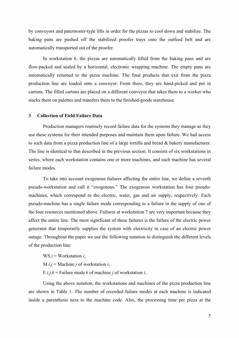
versus the interval times of each class. Figure 1 shows the histograms of TBF, TTR and TTRe
at the entire production line level. The histograms of TBF and TTR exhibit the typical skewed
shape of the Weibull distribution function, whereas the histogram of the TTRe has a double
peak because TTRe is equal to TTR plus an extra time which is added only in case material is
scrapped.
TBF LINE
20181614121086420
700
600
500
400
300
200
100
0
Std. Dev = 1.80 Mean = 1
N = 1772.00
TTR LINE
330290250210170130905010
700
600
500
400
300
200
100
0
Std. Dev = 23.21 Mean = 34
N = 1773.00
TTRe LINE
450400350300250200150100500
700
600
500
400
300
200
100
0
Std. Dev = 49.30 Mean = 72
N = 1773.00
Figure 1: Histograms of TBF, TTR and TTRe for the pizza production line.
4 Computation of Descriptive Statistics from the Failure Data
Descriptive statistics computed from the failure data are very important for drawing
conclusions about the data and may be useful in identifying important failures as well as
identifying or eliminating candidate distributions for TBF, TTR and TTRe. From the records,
we computed several important descriptive statistics of the failure data at the levels of the
failure modes, the machines, the workstations, and finally the entire line. The sample size for
computing the parameters of TBF is one less than the number of failures, whereas the sample
size for computing the parameters of the TTR and TTRe is equal to the number of failures.
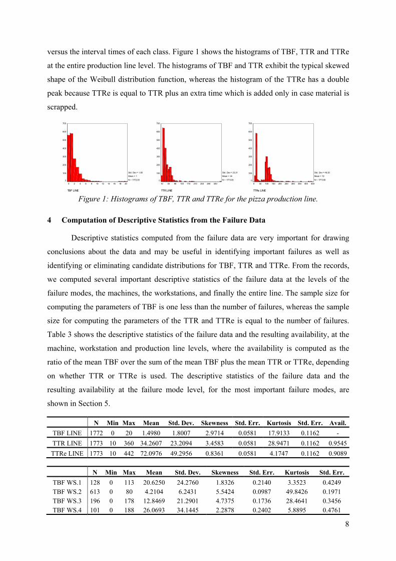
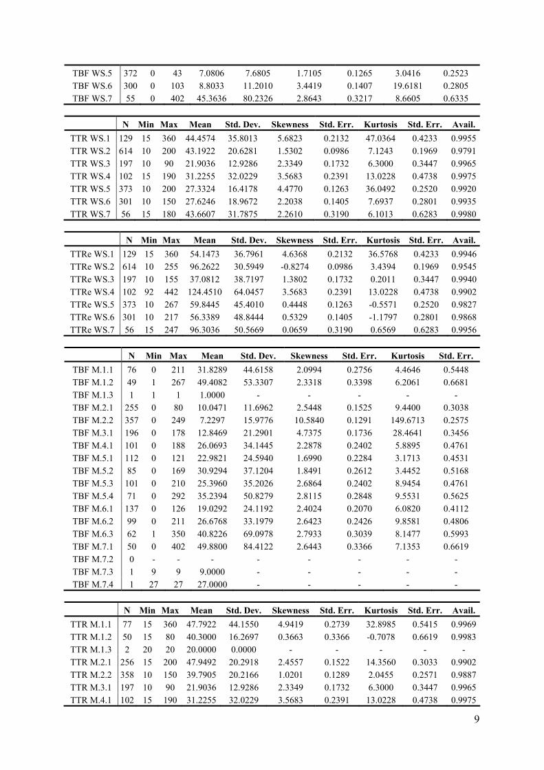
Table 3 shows the descriptive statistics of the failure data and the resulting availability, at the
machine, workstation and production line levels, where the availability is computed as the
ratio of the mean TBF over the sum of the mean TBF plus the mean TTR or TTRe, depending
on whether TTR or TTRe is used. The descriptive statistics of the failure data and the
resulting availability at the failure mode level, for the most important failure modes, are
shown in Section 5.
N Min Max Mean Std. Dev. Skewness Std. Err. Kurtosis Std. Err. Avail. TBF LINE 1772 0 20 1.4980 1.8007 2.9714 0.0581 17.9133 0.1162 - TTR LINE 1773 10 360 34.2607 23.2094 3.4583 0.0581 28.9471 0.1162 0.9545TTRe LINE 1773 10 442 72.0976 49.2956 0.8361 0.0581 4.1747 0.1162 0.9089
N Min Max Mean Std. Dev. Skewness Std. Err. Kurtosis Std. Err.
TBF WS.1 128 0 113 20.6250 24.2760 1.8326 0.2140 3.3523 0.4249 TBF WS.2 613 0 80 4.2104 6.2431 5.5424 0.0987 49.8426 0.1971 TBF WS.3 196 0 178 12.8469 21.2901 4.7375 0.1736 28.4641 0.3456 TBF WS.4 101 0 188 26.0693 34.1445 2.2878 0.2402 5.8895 0.4761
9
TBF WS.5 372 0 43 7.0806 7.6805 1.7105 0.1265 3.0416 0.2523 TBF WS.6 300 0 103 8.8033 11.2010 3.4419 0.1407 19.6181 0.2805 TBF WS.7 55 0 402 45.3636 80.2326 2.8643 0.3217 8.6605 0.6335
N Min Max Mean Std. Dev. Skewness Std. Err. Kurtosis Std. Err. Avail.
TTR WS.1 129 15 360 44.4574 35.8013 5.6823 0.2132 47.0364 0.4233 0.9955TTR WS.2 614 10 200 43.1922 20.6281 1.5302 0.0986 7.1243 0.1969 0.9791TTR WS.3 197 10 90 21.9036 12.9286 2.3349 0.1732 6.3000 0.3447 0.9965TTR WS.4 102 15 190 31.2255 32.0229 3.5683 0.2391 13.0228 0.4738 0.9975TTR WS.5 373 10 200 27.3324 16.4178 4.4770 0.1263 36.0492 0.2520 0.9920TTR WS.6 301 10 150 27.6246 18.9672 2.2038 0.1405 7.6937 0.2801 0.9935TTR WS.7 56 15 180 43.6607 31.7875 2.2610 0.3190 6.1013 0.6283 0.9980
N Min Max Mean Std. Dev. Skewness Std. Err. Kurtosis Std. Err. Avail.
TTRe WS.1 129 15 360 54.1473 36.7961 4.6368 0.2132 36.5768 0.4233 0.9946TTRe WS.2 614 10 255 96.2622 30.5949 -0.8274 0.0986 3.4394 0.1969 0.9545TTRe WS.3 197 10 155 37.0812 38.7197 1.3802 0.1732 0.2011 0.3447 0.9940TTRe WS.4 102 92 442 124.4510 64.0457 3.5683 0.2391 13.0228 0.4738 0.9902TTRe WS.5 373 10 267 59.8445 45.4010 0.4448 0.1263 -0.5571 0.2520 0.9827TTRe WS.6 301 10 217 56.3389 48.8444 0.5329 0.1405 -1.1797 0.2801 0.9868TTRe WS.7 56 15 247 96.3036 50.5669 0.0659 0.3190 0.6569 0.6283 0.9956
N Min Max Mean Std. Dev. Skewness Std. Err. Kurtosis Std. Err.
TBF M.1.1 76 0 211 31.8289 44.6158 2.0994 0.2756 4.4646 0.5448 TBF M.1.2 49 1 267 49.4082 53.3307 2.3318 0.3398 6.2061 0.6681 TBF M.1.3 1 1 1 1.0000 - - - - - TBF M.2.1 255 0 80 10.0471 11.6962 2.5448 0.1525 9.4400 0.3038 TBF M.2.2 357 0 249 7.2297 15.9776 10.5840 0.1291 149.6713 0.2575 TBF M.3.1 196 0 178 12.8469 21.2901 4.7375 0.1736 28.4641 0.3456 TBF M.4.1 101 0 188 26.0693 34.1445 2.2878 0.2402 5.8895 0.4761 TBF M.5.1 112 0 121 22.9821 24.5940 1.6990 0.2284 3.1713 0.4531 TBF M.5.2 85 0 169 30.9294 37.1204 1.8491 0.2612 3.4452 0.5168 TBF M.5.3 101 0 210 25.3960 35.2026 2.6864 0.2402 8.9454 0.4761 TBF M.5.4 71 0 292 35.2394 50.8279 2.8115 0.2848 9.5531 0.5625 TBF M.6.1 137 0 126 19.0292 24.1192 2.4024 0.2070 6.0820 0.4112 TBF M.6.2 99 0 211 26.6768 33.1979 2.6423 0.2426 9.8581 0.4806 TBF M.6.3 62 1 350 40.8226 69.0978 2.7933 0.3039 8.1477 0.5993 TBF M.7.1 50 0 402 49.8800 84.4122 2.6443 0.3366 7.1353 0.6619 TBF M.7.2 0 - - - - - - - - TBF M.7.3 1 9 9 9.0000 - - - - - TBF M.7.4 1 27 27 27.0000 - - - - -
N Min Max Mean Std. Dev. Skewness Std. Err. Kurtosis Std. Err. Avail.
TTR M.1.1 77 15 360 47.7922 44.1550 4.9419 0.2739 32.8985 0.5415 0.9969TTR M.1.2 50 15 80 40.3000 16.2697 0.3663 0.3366 -0.7078 0.6619 0.9983TTR M.1.3 2 20 20 20.0000 0.0000 - - - - - TTR M.2.1 256 15 200 47.9492 20.2918 2.4557 0.1522 14.3560 0.3033 0.9902TTR M.2.2 358 10 150 39.7905 20.2166 1.0201 0.1289 2.0455 0.2571 0.9887TTR M.3.1 197 10 90 21.9036 12.9286 2.3349 0.1732 6.3000 0.3447 0.9965TTR M.4.1 102 15 190 31.2255 32.0229 3.5683 0.2391 13.0228 0.4738 0.9975
10
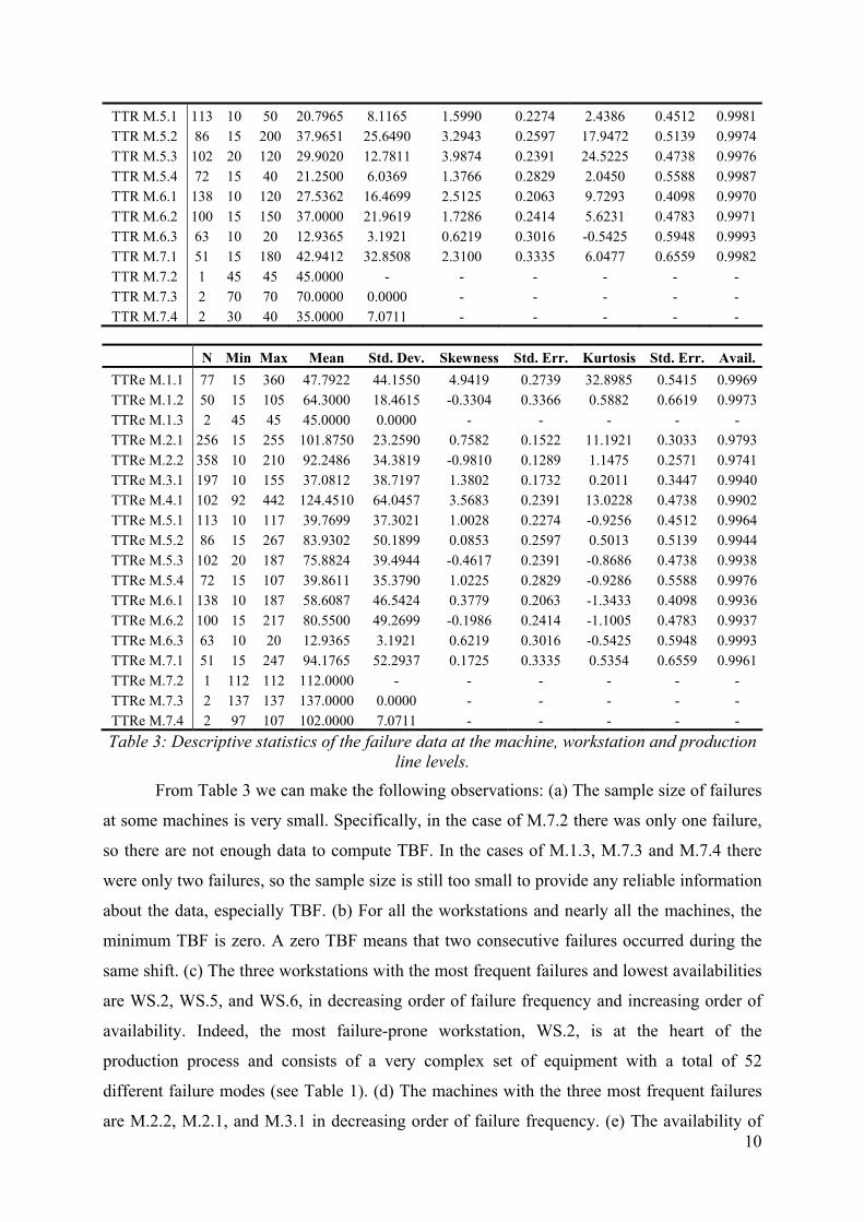
TTR M.5.1 113 10 50 20.7965 8.1165 1.5990 0.2274 2.4386 0.4512 0.9981TTR M.5.2 86 15 200 37.9651 25.6490 3.2943 0.2597 17.9472 0.5139 0.9974TTR M.5.3 102 20 120 29.9020 12.7811 3.9874 0.2391 24.5225 0.4738 0.9976TTR M.5.4 72 15 40 21.2500 6.0369 1.3766 0.2829 2.0450 0.5588 0.9987TTR M.6.1 138 10 120 27.5362 16.4699 2.5125 0.2063 9.7293 0.4098 0.9970TTR M.6.2 100 15 150 37.0000 21.9619 1.7286 0.2414 5.6231 0.4783 0.9971TTR M.6.3 63 10 20 12.9365 3.1921 0.6219 0.3016 -0.5425 0.5948 0.9993TTR M.7.1 51 15 180 42.9412 32.8508 2.3100 0.3335 6.0477 0.6559 0.9982TTR M.7.2 1 45 45 45.0000 - - - - - - TTR M.7.3 2 70 70 70.0000 0.0000 - - - - - TTR M.7.4 2 30 40 35.0000 7.0711 - - - - -
N Min Max Mean Std. Dev. Skewness Std. Err. Kurtosis Std. Err. Avail.
TTRe M.1.1 77 15 360 47.7922 44.1550 4.9419 0.2739 32.8985 0.5415 0.9969TTRe M.1.2 50 15 105 64.3000 18.4615 -0.3304 0.3366 0.5882 0.6619 0.9973TTRe M.1.3 2 45 45 45.0000 0.0000 - - - - - TTRe M.2.1 256 15 255 101.8750 23.2590 0.7582 0.1522 11.1921 0.3033 0.9793TTRe M.2.2 358 10 210 92.2486 34.3819 -0.9810 0.1289 1.1475 0.2571 0.9741TTRe M.3.1 197 10 155 37.0812 38.7197 1.3802 0.1732 0.2011 0.3447 0.9940TTRe M.4.1 102 92 442 124.4510 64.0457 3.5683 0.2391 13.0228 0.4738 0.9902TTRe M.5.1 113 10 117 39.7699 37.3021 1.0028 0.2274 -0.9256 0.4512 0.9964TTRe M.5.2 86 15 267 83.9302 50.1899 0.0853 0.2597 0.5013 0.5139 0.9944TTRe M.5.3 102 20 187 75.8824 39.4944 -0.4617 0.2391 -0.8686 0.4738 0.9938TTRe M.5.4 72 15 107 39.8611 35.3790 1.0225 0.2829 -0.9286 0.5588 0.9976TTRe M.6.1 138 10 187 58.6087 46.5424 0.3779 0.2063 -1.3433 0.4098 0.9936TTRe M.6.2 100 15 217 80.5500 49.2699 -0.1986 0.2414 -1.1005 0.4783 0.9937TTRe M.6.3 63 10 20 12.9365 3.1921 0.6219 0.3016 -0.5425 0.5948 0.9993TTRe M.7.1 51 15 247 94.1765 52.2937 0.1725 0.3335 0.5354 0.6559 0.9961TTRe M.7.2 1 112 112 112.0000 - - - - - - TTRe M.7.3 2 137 137 137.0000 0.0000 - - - - - TTRe M.7.4 2 97 107 102.0000 7.0711 - - - - - Table 3: Descriptive statistics of the failure data at the machine, workstation and production
line levels.
From Table 3 we can make the following observations: (a) The sample size of failures
at some machines is very small. Specifically, in the case of M.7.2 there was only one failure,
so there are not enough data to compute TBF. In the cases of M.1.3, M.7.3 and M.7.4 there
were only two failures, so the sample size is still too small to provide any reliable information
about the data, especially TBF. (b) For all the workstations and nearly all the machines, the
minimum TBF is zero. A zero TBF means that two consecutive failures occurred during the
same shift. (c) The three workstations with the most frequent failures and lowest availabilities
are WS.2, WS.5, and WS.6, in decreasing order of failure frequency and increasing order of
availability. Indeed, the most failure-prone workstation, WS.2, is at the heart of the
production process and consists of a very complex set of equipment with a total of 52
different failure modes (see Table 1). (d) The machines with the three most frequent failures
are M.2.2, M.2.1, and M.3.1 in decreasing order of failure frequency. (e) The availability of
11
the entire line is 95.45%, when it is computed based on the mean TTR. If it computed is based
on the mean TTRe, however, its value drops to 90.89%.
In addition to the gap in production caused by TTRe, a twenty-minute break takes
place at the turn of every eight-hour shift to allow workers to move in and out of the shift,
causing an extra 4.16% drop in the production rate of the line. With this in mind, the ratio of
the effective production rate to the nominal production rate becomes (90.89%)(100% –
4.16%) = 87.11%. This ratio agrees with the 87% output efficiency of the line, which was
computed from the company’s production output records that were collected independently of
the failure data. The agreement between the two numbers validates the collection and analysis
of the failure data.
5 Identification of the Most Important Failures
From the descriptive statistics of the failure data at the failure mode level, which were
not included in Table 3 due to space considerations, we identified the most important failure
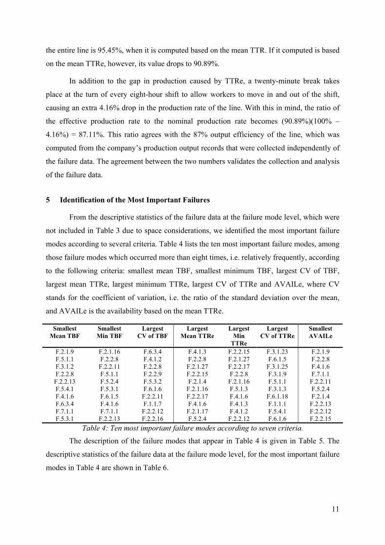
modes according to several criteria. Table 4 lists the ten most important failure modes, among
those failure modes which occurred more than eight times, i.e. relatively frequently, according
to the following criteria: smallest mean TBF, smallest minimum TBF, largest CV of TBF,
largest mean TTRe, largest minimum TTRe, largest CV of TTRe and AVAILe, where CV
stands for the coefficient of variation, i.e. the ratio of the standard deviation over the mean,
and AVAILe is the availability based on the mean TTRe.
Smallest Mean TBF
Smallest Min TBF
Largest CV of TBF
Largest Mean TTRe
Largest Min
TTRe
Largest CV of TTRe
Smallest AVAILe
F.2.1.9 F.2.1.16 F.6.3.4 F.4.1.3 F.2.2.15 F.3.1.23 F.2.1.9 F.5.1.1 F.2.2.8 F.4.1.2 F.2.2.8 F.2.1.27 F.6.1.5 F.2.2.8 F.3.1.2 F.2.2.11 F.2.2.8 F.2.1.27 F.2.2.17 F.3.1.25 F.4.1.6 F.2.2.8 F.5.1.1 F.2.2.9 F.2.2.15 F.2.2.8 F.3.1.9 F.7.1.1 F.2.2.13 F.5.2.4 F.5.3.2 F.2.1.4 F.2.1.16 F.5.1.1 F.2.2.11 F.5.4.1 F.5.3.1 F.6.1.6 F.2.1.16 F.5.1.3 F.3.1.3 F.5.2.4 F.4.1.6 F.6.1.5 F.2.2.11 F.2.2.17 F.4.1.6 F.6.1.18 F.2.1.4 F.6.3.4 F.4.1.6 F.1.1.7 F.4.1.6 F.4.1.3 F.1.1.1 F.2.2.13 F.7.1.1 F.7.1.1 F.2.2.12 F.2.1.17 F.4.1.2 F.5.4.1 F.2.2.12 F.5.3.1 F.2.2.13 F.2.2.16 F.5.2.4 F.2.2.12 F.6.1.6 F.2.2.15
Table 4: Ten most important failure modes according to seven criteria.
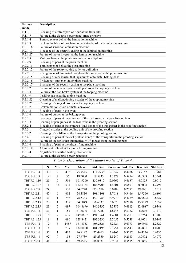
The description of the failure modes that appear in Table 4 is given in Table 5. The
descriptive statistics of the failure data at the failure mode level, for the most important failure
modes in Table 4 are shown in Table 6.
12
Failure mode
Description
F.1.1.1 Blocking of air transport of flour at the flour silo F.1.1.7 Failure at the electric power panel (fuse or relay) F.2.1.4 Torn conveyor belt at the lamination machine F.2.1.9 Broken double motion-chain in the extruder of the lamination machine F.2.1.16 Failure of sensor at lamination machine F.2.1.17 Blockage of the security casing at the lamination machine F.2.1.27 Failure of motor inverter at the lamination machine F.2.2.8 Motion-chain at the pizza machine is out-of-phase F.2.2.9 Blocking of pans at the pizza machine F.2.2.11 Torn conveyor belt at the pizza machine F.2.2.12 Failure of the rotary cutting roller or guillotine F.2.2.13 Realignment of laminated dough on the conveyor at the pizza machine F.2.2.15 Blocking of mechanism that lays pizzas onto metal baking pans F.2.2.16 Broken belt stretcher under pizza machine F.2.2.17 Blockage of the security casing at the pizza machine F.3.1.2 Failure of pneumatic system with pistons at the topping machine F.3.1.3 Failure at the pan brake-system at the topping machine F.3.1.9 Leaking gasket at the toping machine F.3.1.23 Cleaning of malfunctioning nozzles of the topping machine F.3.1.25 Cleaning of clogged nozzles at the topping machine F.4.1.2 Broken motion-chain of metal conveyor F.4.1.3 Blocking of pans in the oven F.4.1.6 Failure of burner at the baking oven F.5.1.1 Blocking of pans at the entrance of the load zone in the proofing section F.5.1.3 Bending of pan guides at the load zone in the proofing section F.5.2.4 Blocking of pans at the entrance (load zone) of the transporter in the proofing section F.5.3.1 Clogged nozzles at the cooling unit of the proofing section F.5.3.2 Cleaning of air filters at the transporter in the proofing section F.5.4.1 Blocking of pans at the exit (unload zone) of the transporter in the proofing section F.6.1.5 Failure of the forks that automatically lift pizzas from the baking pans F.6.1.6 Blocking of pans at the pizza lifting machine F.6.1.18 Alignment of head at the pizza lifting machine F.6.3.4 Adjustment of carton sealing mechanism F.7.1.1 Failure at the electric power generator
Table 5: Description of the failure modes of Table 4.
N Min Max Mean Std. Dev. Skewness Std. Err. Kurtosis Std. Err.TBF F.2.1.4 33 2 432 75.4545 114.2738 2.1247 0.4086 3.7152 0.7984 TBF F.2.1.9 14 2 56 18.5000 18.5835 1.1272 0.5974 0.0308 1.1541
TBF F.2.1.16 25 0 506 101.9200 137.0812 2.0767 0.4637 4.0875 0.9017 TBF F.2.1.27 11 13 531 172.6364 184.9904 1.4201 0.6607 0.8098 1.2794 TBF F.2.2.8 74 0 531 34.5270 75.1676 5.0789 0.2792 29.0601 0.5517
TBF F.2.2.11 47 0 612 54.3830 108.1168 3.7018 0.3466 15.9266 0.6809 TBF F.2.2.12 30 1 798 78.5333 152.1784 3.9972 0.4269 18.0802 0.8327 TBF F.2.2.13 73 1 339 34.6849 56.6737 3.6570 0.2810 15.8229 0.5552 TBF F.2.2.15 23 2 697 104.8696 146.3332 3.2382 0.4813 12.6987 0.9348 TBF F.3.1.2 39 1 151 31.3846 31.7736 1.8748 0.3782 4.2639 0.7410
TBF F.3.1.23 15 7 637 149.0667 194.1261 1.4581 0.5801 1.3264 1.1209 TBF F.3.1.25 19 1 690 128.8421 192.3236 2.2057 0.5238 4.4051 1.0143 TBF F.4.1.2 12 3 1457 181.8333 408.2526 3.2724 0.6373 10.9948 1.2322 TBF F.4.1.3 16 3 739 132.0000 181.2196 2.7954 0.5643 8.9891 1.0908 TBF F.4.1.6 55 1 415 46.8182 77.4465 3.6167 0.3217 14.4374 0.6335 TBF F.5.1.1 92 0 153 27.6739 29.2350 1.8240 0.2513 3.9402 0.4977 TBF F.5.2.4 44 0 418 59.4545 86.0931 2.9634 0.3575 9.8865 0.7017
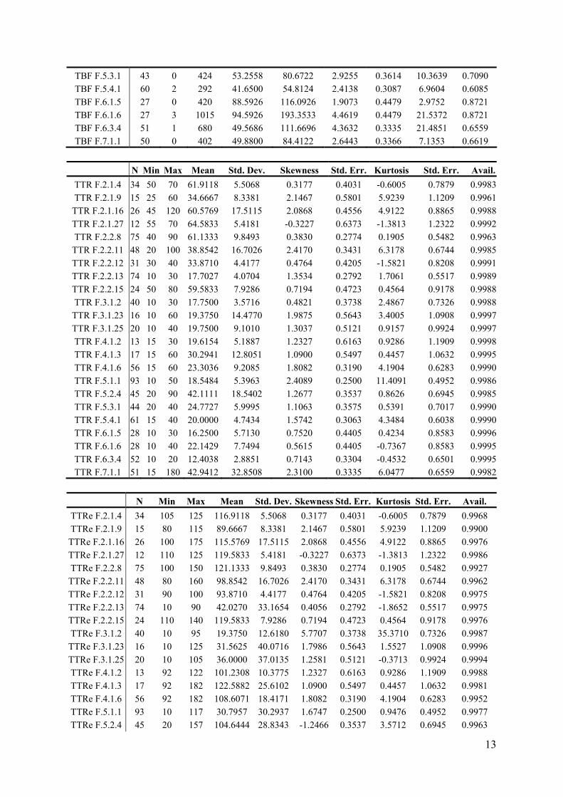
13
TBF F.5.3.1 43 0 424 53.2558 80.6722 2.9255 0.3614 10.3639 0.7090 TBF F.5.4.1 60 2 292 41.6500 54.8124 2.4138 0.3087 6.9604 0.6085 TBF F.6.1.5 27 0 420 88.5926 116.0926 1.9073 0.4479 2.9752 0.8721 TBF F.6.1.6 27 3 1015 94.5926 193.3533 4.4619 0.4479 21.5372 0.8721 TBF F.6.3.4 51 1 680 49.5686 111.6696 4.3632 0.3335 21.4851 0.6559 TBF F.7.1.1 50 0 402 49.8800 84.4122 2.6443 0.3366 7.1353 0.6619
N Min Max Mean Std. Dev. Skewness Std. Err. Kurtosis Std. Err. Avail.
TTRe F.2.1.4 34 105 125 116.9118 5.5068 0.3177 0.4031 -0.6005 0.7879 0.9968 TTRe F.2.1.9 15 80 115 89.6667 8.3381 2.1467 0.5801 5.9239 1.1209 0.9900 TTRe F.2.1.16 26 100 175 115.5769 17.5115 2.0868 0.4556 4.9122 0.8865 0.9976 TTRe F.2.1.27 12 110 125 119.5833 5.4181 -0.3227 0.6373 -1.3813 1.2322 0.9986 TTRe F.2.2.8 75 100 150 121.1333 9.8493 0.3830 0.2774 0.1905 0.5482 0.9927 TTRe F.2.2.11 48 80 160 98.8542 16.7026 2.4170 0.3431 6.3178 0.6744 0.9962 TTRe F.2.2.12 31 90 100 93.8710 4.4177 0.4764 0.4205 -1.5821 0.8208 0.9975 TTRe F.2.2.13 74 10 90 42.0270 33.1654 0.4056 0.2792 -1.8652 0.5517 0.9975 TTRe F.2.2.15 24 110 140 119.5833 7.9286 0.7194 0.4723 0.4564 0.9178 0.9976 TTRe F.3.1.2 40 10 95 19.3750 12.6180 5.7707 0.3738 35.3710 0.7326 0.9987 TTRe F.3.1.23 16 10 125 31.5625 40.0716 1.7986 0.5643 1.5527 1.0908 0.9996 TTRe F.3.1.25 20 10 105 36.0000 37.0135 1.2581 0.5121 -0.3713 0.9924 0.9994 TTRe F.4.1.2 13 92 122 101.2308 10.3775 1.2327 0.6163 0.9286 1.1909 0.9988 TTRe F.4.1.3 17 92 182 122.5882 25.6102 1.0900 0.5497 0.4457 1.0632 0.9981 TTRe F.4.1.6 56 92 182 108.6071 18.4171 1.8082 0.3190 4.1904 0.6283 0.9952 TTRe F.5.1.1 93 10 117 30.7957 30.2937 1.6747 0.2500 0.9476 0.4952 0.9977 TTRe F.5.2.4 45 20 157 104.6444 28.8343 -1.2466 0.3537 3.5712 0.6945 0.9963
N Min Max Mean Std. Dev. Skewness Std. Err. Kurtosis Std. Err. Avail.TTR F.2.1.4 34 50 70 61.9118 5.5068 0.3177 0.4031 -0.6005 0.7879 0.9983TTR F.2.1.9 15 25 60 34.6667 8.3381 2.1467 0.5801 5.9239 1.1209 0.9961
TTR F.2.1.16 26 45 120 60.5769 17.5115 2.0868 0.4556 4.9122 0.8865 0.9988TTR F.2.1.27 12 55 70 64.5833 5.4181 -0.3227 0.6373 -1.3813 1.2322 0.9992TTR F.2.2.8 75 40 90 61.1333 9.8493 0.3830 0.2774 0.1905 0.5482 0.9963
TTR F.2.2.11 48 20 100 38.8542 16.7026 2.4170 0.3431 6.3178 0.6744 0.9985TTR F.2.2.12 31 30 40 33.8710 4.4177 0.4764 0.4205 -1.5821 0.8208 0.9991TTR F.2.2.13 74 10 30 17.7027 4.0704 1.3534 0.2792 1.7061 0.5517 0.9989TTR F.2.2.15 24 50 80 59.5833 7.9286 0.7194 0.4723 0.4564 0.9178 0.9988TTR F.3.1.2 40 10 30 17.7500 3.5716 0.4821 0.3738 2.4867 0.7326 0.9988
TTR F.3.1.23 16 10 60 19.3750 14.4770 1.9875 0.5643 3.4005 1.0908 0.9997TTR F.3.1.25 20 10 40 19.7500 9.1010 1.3037 0.5121 0.9157 0.9924 0.9997TTR F.4.1.2 13 15 30 19.6154 5.1887 1.2327 0.6163 0.9286 1.1909 0.9998TTR F.4.1.3 17 15 60 30.2941 12.8051 1.0900 0.5497 0.4457 1.0632 0.9995TTR F.4.1.6 56 15 60 23.3036 9.2085 1.8082 0.3190 4.1904 0.6283 0.9990TTR F.5.1.1 93 10 50 18.5484 5.3963 2.4089 0.2500 11.4091 0.4952 0.9986TTR F.5.2.4 45 20 90 42.1111 18.5402 1.2677 0.3537 0.8626 0.6945 0.9985TTR F.5.3.1 44 20 40 24.7727 5.9995 1.1063 0.3575 0.5391 0.7017 0.9990TTR F.5.4.1 61 15 40 20.0000 4.7434 1.5742 0.3063 4.3484 0.6038 0.9990TTR F.6.1.5 28 10 30 16.2500 5.7130 0.7520 0.4405 0.4234 0.8583 0.9996TTR F.6.1.6 28 10 40 22.1429 7.7494 0.5615 0.4405 -0.7367 0.8583 0.9995TTR F.6.3.4 52 10 20 12.4038 2.8851 0.7143 0.3304 -0.4532 0.6501 0.9995TTR F.7.1.1 51 15 180 42.9412 32.8508 2.3100 0.3335 6.0477 0.6559 0.9982
14
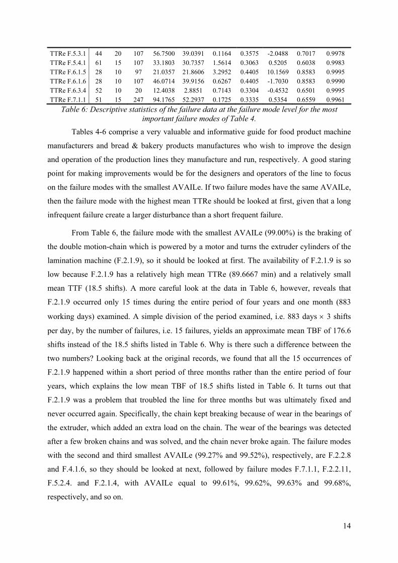
TTRe F.5.3.1 44 20 107 56.7500 39.0391 0.1164 0.3575 -2.0488 0.7017 0.9978 TTRe F.5.4.1 61 15 107 33.1803 30.7357 1.5614 0.3063 0.5205 0.6038 0.9983 TTRe F.6.1.5 28 10 97 21.0357 21.8606 3.2952 0.4405 10.1569 0.8583 0.9995 TTRe F.6.1.6 28 10 107 46.0714 39.9156 0.6267 0.4405 -1.7030 0.8583 0.9990 TTRe F.6.3.4 52 10 20 12.4038 2.8851 0.7143 0.3304 -0.4532 0.6501 0.9995 TTRe F.7.1.1 51 15 247 94.1765 52.2937 0.1725 0.3335 0.5354 0.6559 0.9961
Table 6: Descriptive statistics of the failure data at the failure mode level for the most important failure modes of Table 4.
Tables 4-6 comprise a very valuable and informative guide for food product machine
manufacturers and bread & bakery products manufactures who wish to improve the design
and operation of the production lines they manufacture and run, respectively. A good staring
point for making improvements would be for the designers and operators of the line to focus
on the failure modes with the smallest AVAILe. If two failure modes have the same AVAILe,
then the failure mode with the highest mean TTRe should be looked at first, given that a long
infrequent failure create a larger disturbance than a short frequent failure.
From Table 6, the failure mode with the smallest AVAILe (99.00%) is the braking of
the double motion-chain which is powered by a motor and turns the extruder cylinders of the
lamination machine (F.2.1.9), so it should be looked at first. The availability of F.2.1.9 is so
low because F.2.1.9 has a relatively high mean TTRe (89.6667 min) and a relatively small
mean TTF (18.5 shifts). A more careful look at the data in Table 6, however, reveals that
F.2.1.9 occurred only 15 times during the entire period of four years and one month (883
working days) examined. A simple division of the period examined, i.e. 883 days × 3 shifts
per day, by the number of failures, i.e. 15 failures, yields an approximate mean TBF of 176.6
shifts instead of the 18.5 shifts listed in Table 6. Why is there such a difference between the
two numbers? Looking back at the original records, we found that all the 15 occurrences of
F.2.1.9 happened within a short period of three months rather than the entire period of four
years, which explains the low mean TBF of 18.5 shifts listed in Table 6. It turns out that
F.2.1.9 was a problem that troubled the line for three months but was ultimately fixed and
never occurred again. Specifically, the chain kept breaking because of wear in the bearings of
the extruder, which added an extra load on the chain. The wear of the bearings was detected
after a few broken chains and was solved, and the chain never broke again. The failure modes
with the second and third smallest AVAILe (99.27% and 99.52%), respectively, are F.2.2.8
and F.4.1.6, so they should be looked at next, followed by failure modes F.7.1.1, F.2.2.11,
F.5.2.4. and F.2.1.4, with AVAILe equal to 99.61%, 99.62%, 99.63% and 99.68%,
respectively, and so on.
15
From Tables 4-6 it can be seen that some failures occur very frequently but are not
among the top ten failures according to the smallest AVAILe criterion, because they have
very short repair times. A typical example is the blocking of pans at various parts of the line
(e.g., F.5.1.1, F.5.2.4 and F.5.4.1). The blocking of pans is primarily due to the failure of the
appropriate sensor to count the pans because they may be slightly deformed. When the
problem becomes more acute, the deformed pans are either repaired or replaced. Other
examples of frequent failures with fast repair times are the minor adjustment or cleaning of
equipment (e.g., F.6.3.4 and F.5.3.1). From Tables 4-6, it can also be seen that some failures
have very long repair times but are not among the top ten failures according to the smallest
AVAILe criterion either, because they do not occur very frequently. A typical example is the
blocking of pans in the oven (F.4.1.3), which occurs at a very difficult place to reach and
requires shutting down and restarting the oven. Another example is the failure of an inverter
in one the motors in the lamination machine, which requires disconnecting the failed inverter
from the electric panel of the motor and connecting a new inverter.
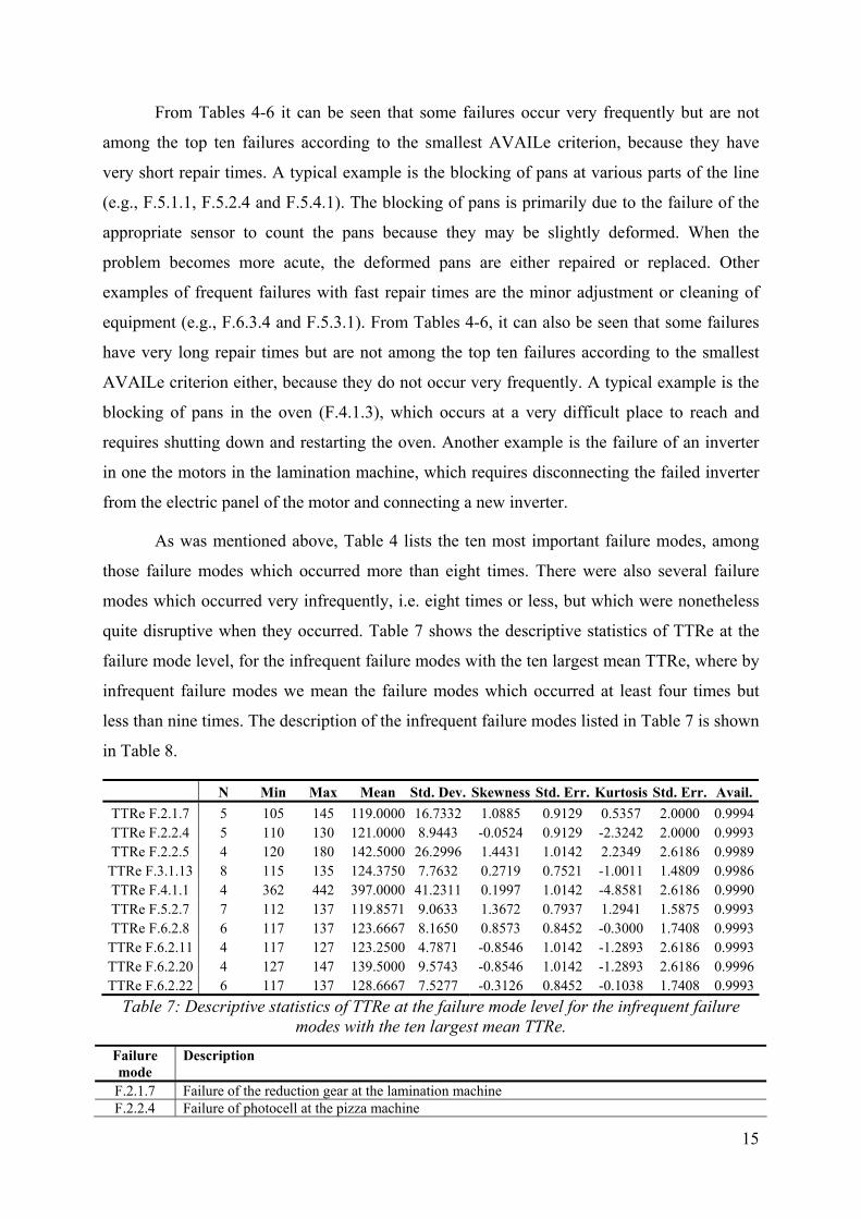
As was mentioned above, Table 4 lists the ten most important failure modes, among
those failure modes which occurred more than eight times. There were also several failure
modes which occurred very infrequently, i.e. eight times or less, but which were nonetheless
quite disruptive when they occurred. Table 7 shows the descriptive statistics of TTRe at the
failure mode level, for the infrequent failure modes with the ten largest mean TTRe, where by
infrequent failure modes we mean the failure modes which occurred at least four times but
less than nine times. The description of the infrequent failure modes listed in Table 7 is shown
in Table 8.
N Min Max Mean Std. Dev. Skewness Std. Err. Kurtosis Std. Err. Avail.TTRe F.2.1.7 5 105 145 119.0000 16.7332 1.0885 0.9129 0.5357 2.0000 0.9994TTRe F.2.2.4 5 110 130 121.0000 8.9443 -0.0524 0.9129 -2.3242 2.0000 0.9993TTRe F.2.2.5 4 120 180 142.5000 26.2996 1.4431 1.0142 2.2349 2.6186 0.9989TTRe F.3.1.13 8 115 135 124.3750 7.7632 0.2719 0.7521 -1.0011 1.4809 0.9986TTRe F.4.1.1 4 362 442 397.0000 41.2311 0.1997 1.0142 -4.8581 2.6186 0.9990TTRe F.5.2.7 7 112 137 119.8571 9.0633 1.3672 0.7937 1.2941 1.5875 0.9993TTRe F.6.2.8 6 117 137 123.6667 8.1650 0.8573 0.8452 -0.3000 1.7408 0.9993TTRe F.6.2.11 4 117 127 123.2500 4.7871 -0.8546 1.0142 -1.2893 2.6186 0.9993TTRe F.6.2.20 4 127 147 139.5000 9.5743 -0.8546 1.0142 -1.2893 2.6186 0.9996TTRe F.6.2.22 6 117 137 128.6667 7.5277 -0.3126 0.8452 -0.1038 1.7408 0.9993
Table 7: Descriptive statistics of TTRe at the failure mode level for the infrequent failure modes with the ten largest mean TTRe.
Failure mode
Description
F.2.1.7 Failure of the reduction gear at the lamination machine F.2.2.4 Failure of photocell at the pizza machine
16
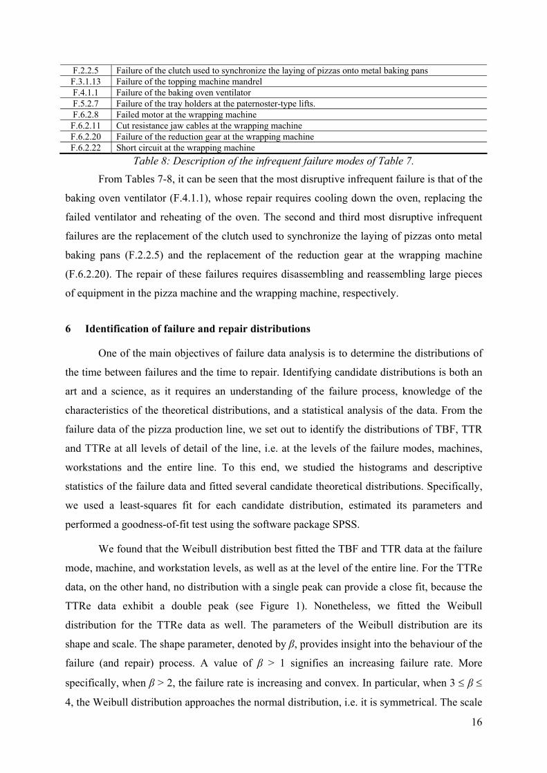
F.2.2.5 Failure of the clutch used to synchronize the laying of pizzas onto metal baking pans F.3.1.13 Failure of the topping machine mandrel F.4.1.1 Failure of the baking oven ventilator F.5.2.7 Failure of the tray holders at the paternoster-type lifts. F.6.2.8 Failed motor at the wrapping machine F.6.2.11 Cut resistance jaw cables at the wrapping machine F.6.2.20 Failure of the reduction gear at the wrapping machine F.6.2.22 Short circuit at the wrapping machine
Table 8: Description of the infrequent failure modes of Table 7.
From Tables 7-8, it can be seen that the most disruptive infrequent failure is that of the
baking oven ventilator (F.4.1.1), whose repair requires cooling down the oven, replacing the
failed ventilator and reheating of the oven. The second and third most disruptive infrequent
failures are the replacement of the clutch used to synchronize the laying of pizzas onto metal
baking pans (F.2.2.5) and the replacement of the reduction gear at the wrapping machine
(F.6.2.20). The repair of these failures requires disassembling and reassembling large pieces
of equipment in the pizza machine and the wrapping machine, respectively.
6 Identification of failure and repair distributions
One of the main objectives of failure data analysis is to determine the distributions of
the time between failures and the time to repair. Identifying candidate distributions is both an
art and a science, as it requires an understanding of the failure process, knowledge of the
characteristics of the theoretical distributions, and a statistical analysis of the data. From the
failure data of the pizza production line, we set out to identify the distributions of TBF, TTR
and TTRe at all levels of detail of the line, i.e. at the levels of the failure modes, machines,
workstations and the entire line. To this end, we studied the histograms and descriptive
statistics of the failure data and fitted several candidate theoretical distributions. Specifically,
we used a least-squares fit for each candidate distribution, estimated its parameters and
performed a goodness-of-fit test using the software package SPSS.
We found that the Weibull distribution best fitted the TBF and TTR data at the failure
mode, machine, and workstation levels, as well as at the level of the entire line. For the TTRe
data, on the other hand, no distribution with a single peak can provide a close fit, because the
TTRe data exhibit a double peak (see Figure 1). Nonetheless, we fitted the Weibull
distribution for the TTRe data as well. The parameters of the Weibull distribution are its
shape and scale. The shape parameter, denoted by β, provides insight into the behaviour of the
failure (and repair) process. A value of β > 1 signifies an increasing failure rate. More
specifically, when β > 2, the failure rate is increasing and convex. In particular, when 3 ≤ β ≤
4, the Weibull distribution approaches the normal distribution, i.e. it is symmetrical. The scale
17
parameter of the Weibull distribution, denoted by θ, influences both the mean and the spread
of the distribution. As θ increases, the reliability at a given point in time increases, whereas
the slope of the hazard rate decreases (Ebeling, 1997).
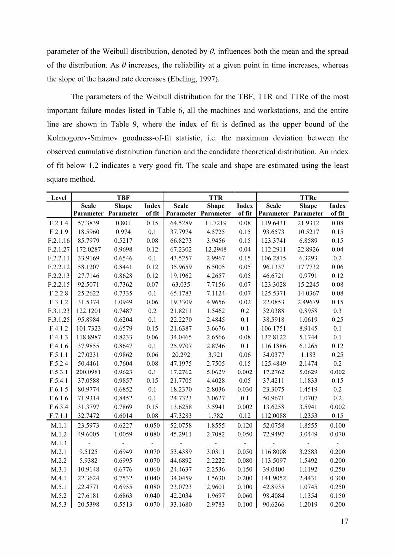
The parameters of the Weibull distribution for the TBF, TTR and TTRe of the most
important failure modes listed in Table 6, all the machines and workstations, and the entire
line are shown in Table 9, where the index of fit is defined as the upper bound of the
Kolmogorov-Smirnov goodness-of-fit statistic, i.e. the maximum deviation between the
observed cumulative distribution function and the candidate theoretical distribution. An index
of fit below 1.2 indicates a very good fit. The scale and shape are estimated using the least
square method.
Level TBF TTR TTRe
Scale
Parameter Shape
Parameter Index of fit
Scale Parameter
Shape Parameter
Indexof fit
Scale Parameter
Shape Parameter
Indexof fit
F.2.1.4 57.3839 0.801 0.15 64.5289 11.7219 0.08 119.6431 21.9312 0.08 F.2.1.9 18.5960 0.974 0.1 37.7974 4.5725 0.15 93.6573 10.5217 0.15 F.2.1.16 85.7979 0.5217 0.08 66.8273 3.9456 0.15 123.3741 6.8589 0.15 F.2.1.27 172.0287 0.9698 0.12 67.2302 12.2948 0.04 112.2911 22.8926 0.04 F.2.2.11 33.9169 0.6546 0.1 43.5257 2.9967 0.15 106.2815 6.3293 0.2 F.2.2.12 58.1207 0.8441 0.12 35.9659 6.5005 0.05 96.1337 17.7732 0.06 F.2.2.13 27.7146 0.8628 0.12 19.1962 4.2657 0.05 46.6721 0.9791 0.12 F.2.2.15 92.5071 0.7362 0.07 63.035 7.7156 0.07 123.3028 15.2245 0.08 F.2.2.8 25.2622 0.7335 0.1 65.1783 7.1124 0.07 125.5371 14.0367 0.08 F.3.1.2 31.5374 1.0949 0.06 19.3309 4.9656 0.02 22.0853 2.49679 0.15 F.3.1.23 122.1201 0.7487 0.2 21.8211 1.5462 0.2 32.0388 0.8958 0.3 F.3.1.25 95.8984 0.6204 0.1 22.2270 2.4845 0.1 38.5918 1.0619 0.25 F.4.1.2 101.7323 0.6579 0.15 21.6387 3.6676 0.1 106.1751 8.9145 0.1 F.4.1.3 118.8987 0.8233 0.06 34.0465 2.6566 0.08 132.8122 5.1744 0.1 F.4.1.6 37.9855 0.8647 0.1 25.9707 2.8746 0.1 116.1886 6.1265 0.12 F.5.1.1 27.0231 0.9862 0.06 20.292 3.921 0.06 34.0377 1.183 0.25 F.5.2.4 50.4461 0.7604 0.08 47.1975 2.7505 0.15 125.4849 2.1474 0.2 F.5.3.1 200.0981 0.9623 0.1 17.2762 5.0629 0.002 17.2762 5.0629 0.002 F.5.4.1 37.0588 0.9857 0.15 21.7705 4.4028 0.05 37.4211 1.1833 0.15 F.6.1.5 80.9774 0.6852 0.1 18.2370 2.8036 0.030 23.3075 1.4519 0.2 F.6.1.6 71.9314 0.8452 0.1 24.7323 3.0627 0.1 50.9671 1.0707 0.2 F.6.3.4 31.3797 0.7869 0.15 13.6258 3.5941 0.002 13.6258 3.5941 0.002 F.7.1.1 32.7472 0.6014 0.08 47.3283 1.782 0.12 112.0088 1.2353 0.15 M.1.1 23.5973 0.6227 0.050 52.0758 1.8555 0.120 52.0758 1.8555 0.100 M.1.2 49.6005 1.0059 0.080 45.2911 2.7082 0.050 72.9497 3.0449 0.070 M.1.3 - - - - - - - - - M.2.1 9.5125 0.6949 0.070 53.4389 3.0311 0.050 116.8008 3.2583 0.200 M.2.2 5.9382 0.6995 0.070 44.6892 2.2222 0.080 113.5097 1.5492 0.200 M.3.1 10.9148 0.6776 0.060 24.4637 2.2536 0.150 39.0400 1.1192 0.250 M.4.1 22.3624 0.7532 0.040 34.0459 1.5630 0.200 141.9052 2.4431 0.300 M.5.1 22.4771 0.6955 0.080 23.0723 2.9601 0.100 42.8935 1.0745 0.250 M.5.2 27.6181 0.6863 0.040 42.2034 1.9697 0.060 98.4084 1.1354 0.150 M.5.3 20.5398 0.5513 0.070 33.1680 2.9783 0.100 90.6266 1.2019 0.200
18
M.5.4 30.3546 0.7525 0.070 23.3516 3.7846 0.070 44.3798 1.1177 0.150 M.6.1 17.1183 0.7755 0.060 30.6924 2.2242 0.080 63.7904 1.0917 0.150 M.6.2 24.0122 0.6911 0.050 41.4618 1.9753 0.100 93.5395 1.1287 0.150 M.6.3 29.6937 0.8202 0.120 14.2368 3.5502 0.006 14.2368 3.5502 0.006 WS.1 18.4310 0.7801 0.040 48.9663 2.0909 0.100 60.2041 2.1178 0.040 WS.2 3.7535 0.6984 0.060 48.4866 2.4387 0.060 117.4583 1.8533 0.250 WS.3 10.9148 0.6776 0.060 24.4637 2.2536 0.150 39.0400 1.1192 0.250 WS.4 22.3624 0.7532 0.040 34.0459 1.5630 0.200 141.9052 2.4431 0.300 WS.5 6.7914 0.7099 0.040 30.3919 2.4196 0.100 66.3262 1.1042 0.150 WS.6 8.5246 0.7248 0.050 30.5721 1.8638 0.100 59.3088 1.0105 0.200 WS.7 28.5554 0.6085 0.070 48.2671 1.8481 0.150 115.4226 1.2791 0.150 LINE 1.4182 0.6941 0.050 37.9572 2.0142 0.080 81.1524 1.2081 0.200
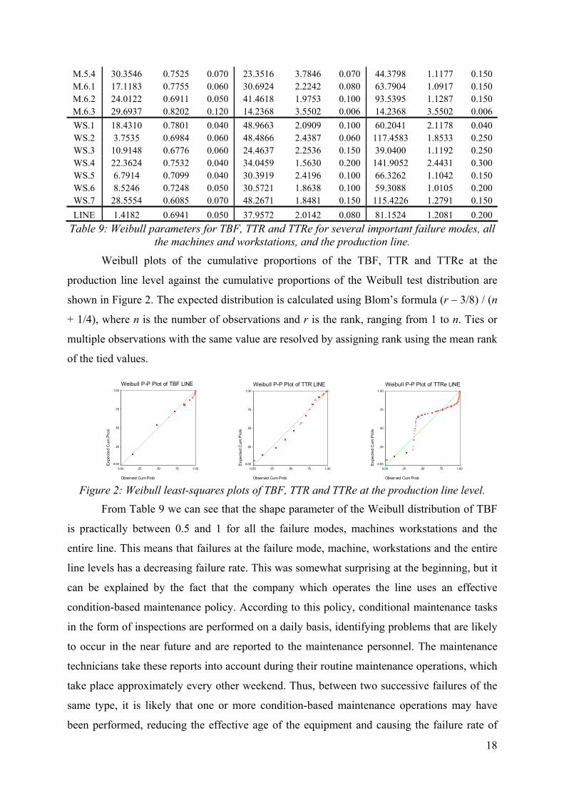
Table 9: Weibull parameters for TBF, TTR and TTRe for several important failure modes, all the machines and workstations, and the production line.
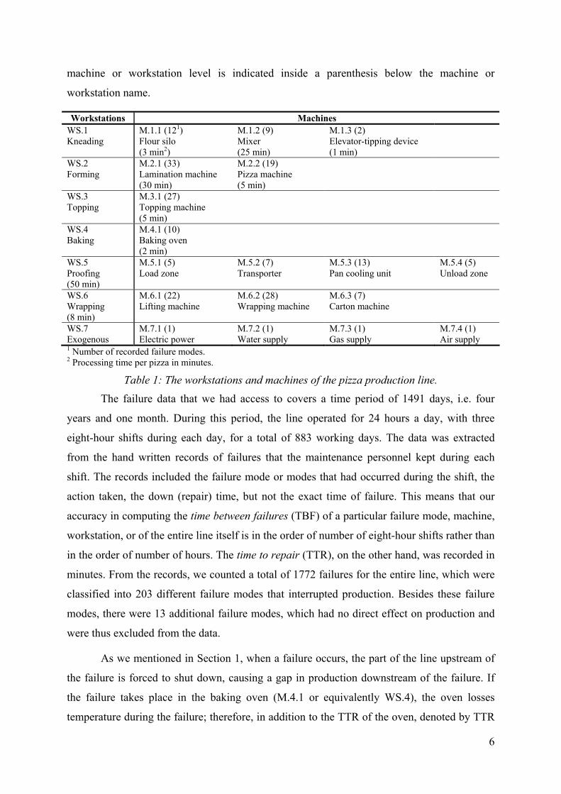
Weibull plots of the cumulative proportions of the TBF, TTR and TTRe at the
production line level against the cumulative proportions of the Weibull test distribution are
shown in Figure 2. The expected distribution is calculated using Blom’s formula (r – 3/8) / (n
+ 1/4), where n is the number of observations and r is the rank, ranging from 1 to n. Ties or
multiple observations with the same value are resolved by assigning rank using the mean rank
of the tied values.
Weibull P-P Plot of TBF LINE
Observed Cum Prob
1.00.75.50.250.00
Exp
ecte
d C
um P
rob
1.00
.75
.50
.25
0.00
Weibull P-P Plot of TTR LINE
Observed Cum Prob
1.00.75.50.250.00
Exp
ecte
d C
um P
rob
1.00
.75
.50
.25
0.00
Weibull P-P Plot of TTRe LINE
Observed Cum Prob
1.00.75.50.250.00
Exp
ecte
d C
um P
rob
1.00
.75
.50
.25
0.00
Figure 2: Weibull least-squares plots of TBF, TTR and TTRe at the production line level.
From Table 9 we can see that the shape parameter of the Weibull distribution of TBF
is practically between 0.5 and 1 for all the failure modes, machines workstations and the
entire line. This means that failures at the failure mode, machine, workstations and the entire
line levels has a decreasing failure rate. This was somewhat surprising at the beginning, but it
can be explained by the fact that the company which operates the line uses an effective
condition-based maintenance policy. According to this policy, conditional maintenance tasks
in the form of inspections are performed on a daily basis, identifying problems that are likely
to occur in the near future and are reported to the maintenance personnel. The maintenance
technicians take these reports into account during their routine maintenance operations, which
take place approximately every other weekend. Thus, between two successive failures of the
same type, it is likely that one or more condition-based maintenance operations may have
been performed, reducing the effective age of the equipment and causing the failure rate of
19
the particular failure type to be decreasing. From Table 9 we can also see that the shape
parameter of the Weibull distribution of TTR and TTRe is greater than one for all the for all
the failure modes, machines, workstations and the entire line. This implies that the repair rates
are increasing. This is natural, because the longer the time since a repair started, the higher the
probability that it will finish soon. In fact, in most cases the shape parameter is greater than
two, which means that the repair rate is increasing and convex.
7 Determination of Degrees of Autocorrelation and Cross Correlation of the Failure
Data
Many analytical models of transfer lines rely on the assumption that the TBF and TTR
of the workstations are independent (e.g., see Buzacott and Shanthikumar, 1993, and
Gershwin, 1994). Inman (1999) presented actual data from two automotive body-welding
lines in order to assess among other things the validity of the independence assumptions for
TBF and TTR. They found that while there is a somewhat statistically significant
autocorrelation in TBF, it may not be practically significant and it does not seem to be of
fundamental importance. Lack of autocorrelation is necessary but not sufficient to show that
successive observations of a random variable are independent. For the purposes of
manufacturing management, however, testing for autocorrelation should suffice as an
indication of independence.
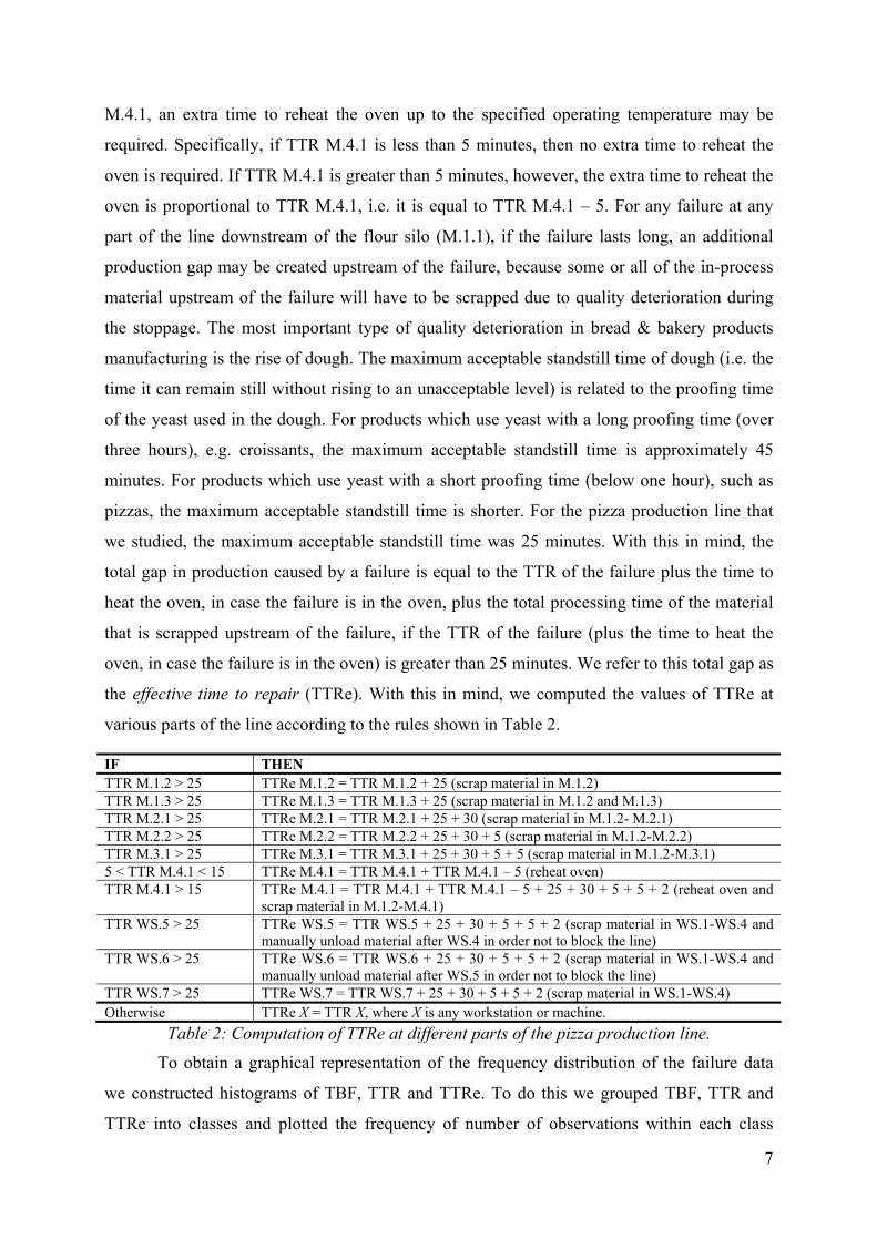
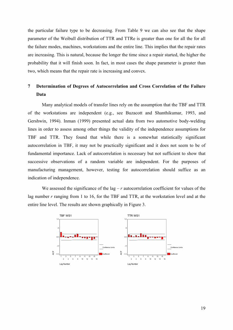
We assessed the significance of the lag – r autocorrelation coefficient for values of the
lag number r ranging from 1 to 16, for the TBF and TTR, at the workstation level and at the
entire line level. The results are shown graphically in Figure 3.
TBF WS1
Lag Number
1615
1413
1211
109
87
65
43
21
ACF
1.0
.5
0.0
-.5
-1.0
Confidence Limits
Coefficient
TTR WS1
Lag Number
1615
1413
1211
109
87
65
43
21
ACF
1.0
.5
0.0
-.5
-1.0
Confidence Limits
Coefficient
20
TBF WS2
Lag Number
1615
1413
1211
109
87
65
43
21
ACF
1.0
.5
0.0
-.5
-1.0
Confidence Limits
Coefficient
TTR WS2
Lag Number
1615
1413
1211
109
87
65
43
21
ACF
1.0
.5
0.0
-.5
-1.0
Confidence Limits
Coefficient
TBF WS3
Lag Number
1615
1413
1211
109
87
65
43
21
ACF
1.0
.5
0.0
-.5
-1.0
Confidence Limits
Coefficient
TTR WS3
Lag Number
1615
1413
1211
109
87
65
43
21
ACF
1.0
.5
0.0
-.5
-1.0
Confidence Limits
Coefficient
TBF WS4
Lag Number
1615
1413
1211
109
87
65
43
21
ACF
1.0
.5
0.0
-.5
-1.0
Confidence Limits
Coefficient
TTR WS4
Lag Number
1615
1413
1211
109
87
65
43
21
ACF
1.0
.5
0.0
-.5
-1.0
Confidence Limits
Coefficient
TBF WS5
Lag Number
1615
1413
1211
109
87
65
43
21
ACF
1.0
.5
0.0
-.5
-1.0
Confidence Limits
Coefficient
TTR WS5
Lag Number
1615
1413
1211
109
87
65
43
21
ACF
1.0
.5
0.0
-.5
-1.0
Confidence Limits
Coefficient
TBF WS6
Lag Number
1615
1413
1211
109
87
65
43
21
ACF
1.0
.5
0.0
-.5
-1.0
Confidence Limits
Coefficient
TTR WS6
Lag Number
1615
1413
1211
109
87
65
43
21
ACF
1.0
.5
0.0
-.5
-1.0
Confidence Limits
Coefficient
21
TBF WS7
Lag Number
1615
1413
1211
109
87
65
43
21
ACF
1.0
.5
0.0
-.5
-1.0
Confidence Limits
Coefficient
TTR WS7
Lag Number
1615
1413
1211
109
87
65
43
21
ACF
1.0
.5
0.0
-.5
-1.0
Confidence Limits
Coefficient
TBF LINE
Lag Number
1615
1413
1211
109
87
65
43
21
ACF
1.0
.5
0.0
-.5
-1.0
Confidence Limits
Coefficient
TTR LINE
Lag Number
1615
1413
1211
109
87
65
43
21
ACF
1.0
.5
0.0
-.5
-1.0
Confidence Limits
Coefficient
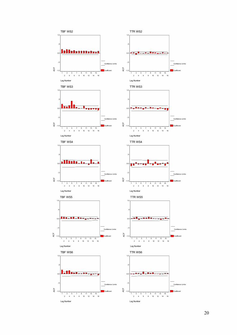
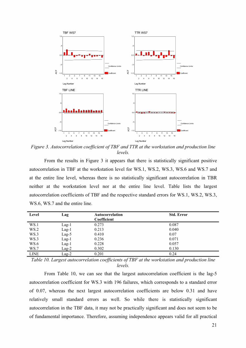
Figure 3. Autocorrelation coefficient of TBF and TTR at the workstation and production line
levels.
From the results in Figure 3 it appears that there is statistically significant positive
autocorrelation in TBF at the workstation level for WS.1, WS.2, WS.3, WS.6 and WS.7 and
at the entire line level, whereas there is no statistically significant autocorrelation in TBR
neither at the workstation level nor at the entire line level. Table lists the largest
autocorrelation coefficients of TBF and the respective standard errors for WS.1, WS.2, WS.3,
WS.6, WS.7 and the entire line.
Level Lag Autocorrelation Coefficient
Std. Error
WS.1 Lag-1 0.273 0.087 WS.2 Lag-1 0.213 0.040 WS.3 Lag-5 0.410 0.07 WS.3 Lag-1 0.236 0.071 WS.6 Lag-1 0.228 0.057 WS.7 Lag-2 0.302 0.130 LINE Lag-2 0.201 0.24 Table 10. Largest autocorrelation coefficients of TBF at the workstation and production line
levels.
From Table 10, we can see that the largest autocorrelation coefficient is the lag-5
autocorrelation coefficient for WS.3 with 196 failures, which corresponds to a standard error
of 0.07, whereas the next largest autocorrelation coefficients are below 0.31 and have
relatively small standard errors as well. So while there is statistically significant
autocorrelation in the TBF data, it may not be practically significant and does not seem to be
of fundamental importance. Therefore, assuming independence appears valid for all practical
22
purposes for both TBF and TTR. These results carry over to the TTRe data too, because
TTRe is strongly positively correlated to TTR since it is equal to TTR plus an extra time
which is added in case TTR is long.
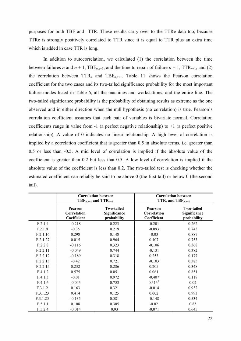
In addition to autocorrelation, we calculated (1) the correlation between the time
between failures n and n + 1, TBFn,n+1, and the time to repair of failure n + 1, TTRn+1, and (2)
the correlation between TTRn and TBFn,n+1. Table 11 shows the Pearson correlation
coefficient for the two cases and its two-tailed significance probability for the most important
failure modes listed in Table 6, all the machines and workstations, and the entire line. The
two-tailed significance probability is the probability of obtaining results as extreme as the one
observed and in either direction when the null hypothesis (no correlation) is true. Pearson’s
correlation coefficient assumes that each pair of variables is bivariate normal. Correlation
coefficients range in value from -1 (a perfect negative relationship) to +1 (a perfect positive
relationship). A value of 0 indicates no linear relationship. A high level of correlation is
implied by a correlation coefficient that is greater than 0.5 in absolute terms, i.e. greater than
0.5 or less than -0.5. A mid level of correlation is implied if the absolute value of the
coefficient is greater than 0.2 but less that 0.5. A low level of correlation is implied if the
absolute value of the coefficient is less than 0.2. The two-tailed test is checking whether the
estimated coefficient can reliably be said to be above 0 (the first tail) or below 0 (the second
tail).
Correlation between TBFn,n+1 and TTRn+1
Correlation between TTRn and TBFn,n+1
Pearson Correlation Coefficient
Two-tailed Significance probability
Pearson Correlation Coefficient
Two-tailed Significance probability
F.2.1.4 -0.218 0.223 -0.201 0.262 F.2.1.9 -0.35 0.219 -0.093 0.743
F.2.1.16 0.298 0.148 -0.03 0.887 F.2.1.27 0.015 0.964 0.107 0.753 F.2.2.8 -0.116 0.323 -0.106 0.368
F.2.2.11 -0.049 0.744 -0.131 0.382 F.2.2.12 -0.189 0.318 0.253 0.177 F.2.2.13 -0.42 0.721 -0.103 0.385 F.2.2.15 0.232 0.286 0.205 0.348 F.4.1.2 0.575 0.051 0.061 0.851 F.4.1.3 -0.01 0.972 -0.407 0.118 F.4.1.6 -0.043 0.753 0.3131 0.02 F.3.1.2 0.163 0.321 -0.014 0.932 F.3.1.23 0.414 0.125 0.002 0.993 F.3.1.25 -0.135 0.581 -0.148 0.534 F.5.1.1 0.108 0.305 -0.02 0.85 F.5.2.4 -0.014 0.93 -0.071 0.645
23
F.5.3.1 -0.009 0.952 -0.136 0.383 F.5.4.1 0.027 0.837 -0.084 0.525 F.6.1.5 -0.056 0.783 -0.215 0.281 F.6.1.6 -0.257 0.195 0.116 0.564 F.6.3.4 -0.164 0.251 0.179 0.209 F.7.1.1 0.025 0.862 0.411 0.003 M.1.1 0.026 0.822 -0.083 0.476 M.1.2 0.032 0.826 -0.135 0.354 M.1.3 --3 - - - M.2.1 -0.058 0.354 -0.029 0.649 M.2.2 -0.04 0.455 0.043 0.422 M.3.1 -0.049 0.496 0.013 0.853 M.4.1 -0.082 0.412 -0.049 0.624 M.5.1 -0.105 0.268 0.004 0.968 M.5.2 0.044 0.692 -0.005 0.96 M.5.3 0.2152 0.031 0.2522 0.011 M.5.4 -0.073 0.544 0.011 0.928 M.6.1 -0.022 0.797 0.096 0.424 M.6.2 0.092 0.365 0.125 0.218 M.6.3 0.042 0.744 0.047 0.718 WS.1 0.016 0.854 -0.004 0.967 WS.2 0.073 0.071 0.015 0.708 WS.3 -0.049 0.496 0.013 0.853 WS.4 -0.082 0.412 -0.049 0.624 WS.5 0.024 0.649 -0.021 0.685 WS.6 -0.025 0.665 -0.069 0.234 WS.7 0.048 0.73 0.4061 0.002 LINE 0.0492 0.039 0.0592 0.013
1 Correlation is significant at the 0.01 level (2-tailed). 2 Correlation is significant at the 0.05 level (2-tailed). 3 Cannot be computed because at least one of the variables is constant.
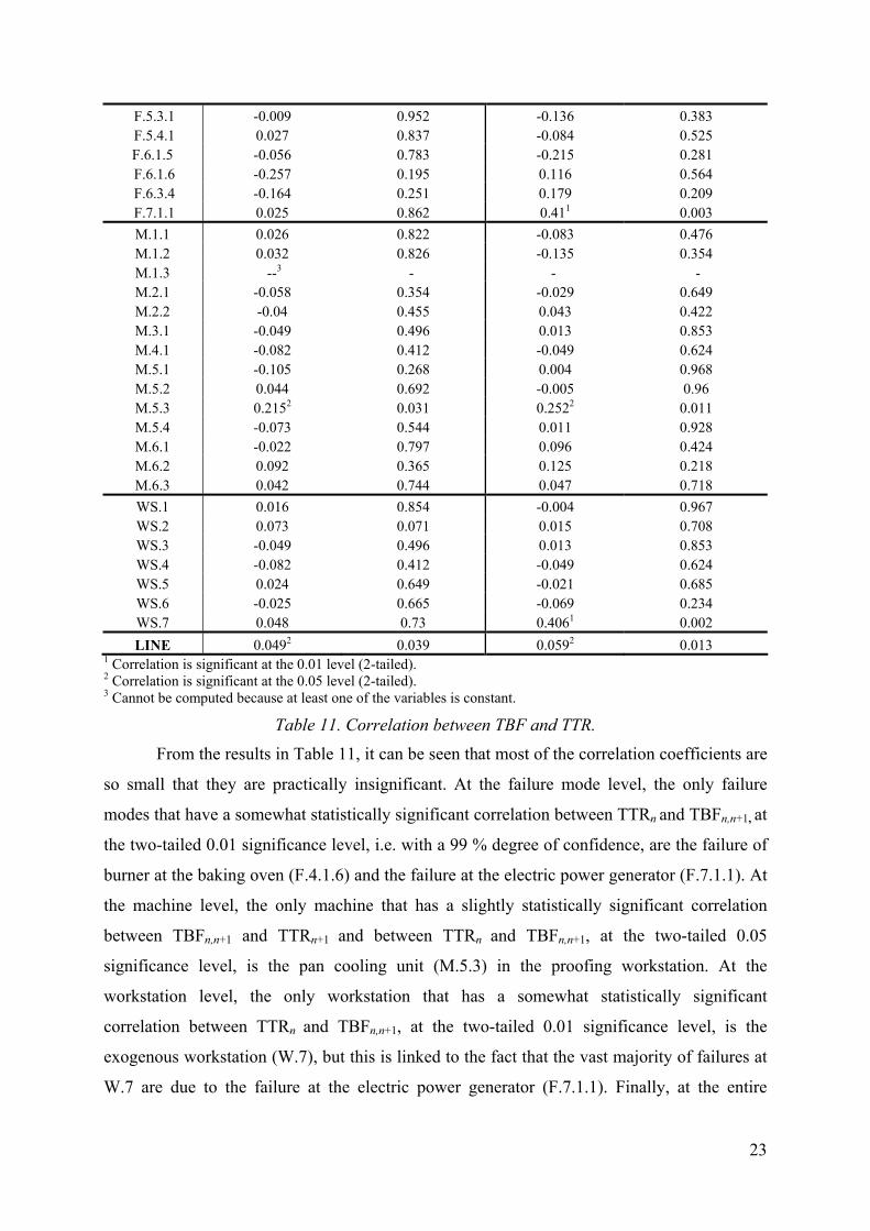
Table 11. Correlation between TBF and TTR.
From the results in Table 11, it can be seen that most of the correlation coefficients are
so small that they are practically insignificant. At the failure mode level, the only failure
modes that have a somewhat statistically significant correlation between TTRn and TBFn,n+1, at
the two-tailed 0.01 significance level, i.e. with a 99 % degree of confidence, are the failure of
burner at the baking oven (F.4.1.6) and the failure at the electric power generator (F.7.1.1). At
the machine level, the only machine that has a slightly statistically significant correlation
between TBFn,n+1 and TTRn+1 and between TTRn and TBFn,n+1, at the two-tailed 0.05
significance level, is the pan cooling unit (M.5.3) in the proofing workstation. At the
workstation level, the only workstation that has a somewhat statistically significant
correlation between TTRn and TBFn,n+1, at the two-tailed 0.01 significance level, is the
exogenous workstation (W.7), but this is linked to the fact that the vast majority of failures at
W.7 are due to the failure at the electric power generator (F.7.1.1). Finally, at the entire
24
production line level, there is a marginally statistically significant correlation between
TBFn,n+1 and TTRn+1 and between TTRn and TBFn,n+1, at the two-tailed 0.05 significance level.
In all the above cases, wherever there is a statistically significant correlation, this
correlation is positive. This is reasonable in the following sense. A positive correlation
coefficient between TBFn,n+1 and TTRn+1 implies that the longer the time between two
failures, the more problems accumulate, and therefore the longer the time it takes to repair the
latter of the two failures. A positive correlation coefficient between TTRn and TBFn,n+1
implies that the more time one spends repairing a failure, the more careful job one does, and
therefore the longer the time until the next failure is. Both implications are intuitively
reasonable.
8 Conclusions
We presented a statistical analysis of failure data of an automated pizza production
line, covering a period of four years. We computed descriptive statistics of the failure data and
we identified the most important failures. We also computed the parameters of the Weibull
distributions that best fit the failure data. We found that failures have a decreasing failure rate,
because between of the condition-based maintenance policy used by the company operating
the line, which means that between any two successive failures of the same type, it is likely
that one or more condition-based maintenance operations may have been performed. Finally,
we investigated the existence of autocorrelations and cross correlations in the failure data. We
found that there is a statistically significant positive autocorrelation in TBF at the workstation
level for WS.1, WS.2, WS.3, WS.6 and WS.7 and at the entire line level, whereas there is no
statistically significant autocorrelation in TBR neither at the workstation level nor at the entire
line level; however the statistically significant autocorrelation in the TBF data may not be
practically significant and does not seem to be of fundamental importance. Therefore,
assuming independence appears valid for all practical purposes for both TBF and TTR. We
also found that at the entire line level, there is a marginally statistically significant, positive
correlation between TBFn,n+1 and TTRn+1 and between TTRn and TBFn,n+1, at the two-tailed
0.05 significance level. This implies that the longer the time between two failures, the more
problems accumulate, and therefore the longer the time it takes to fix the latter failure. It also
implies that the more time one spends fixing a failure, the more careful job one does, and
therefore the longer the time until the next failure is.
25
References
Baker, R.D. (2001). Data-based modelling of the failure rate of repairable equipment. Lifetime
Data Analysis, 7, 65-83.
Buzacott, J.A. and Shanthikumar, J.G. (1993). Stochastic models of manufacturing systems,
Prentice Hall, Englewood Cliffs, NJ.
Coit, D.W. and Jin, T. (2000). Gamma distribution parameter estimation for field reliability
data with missing failure times, IIE Transactions, 32, 1161-1166.
Edeling, C.E. (1997). An Introduction to Reliability and Maintainability Engineering.
McGraw Hill, New York, NY.
Freeman, J.M. (1996). Analysing equipment failure rates. International Journal of Quality &
Reliability Management, 13(4), 39-49.
Gershwin, S.B. (1994). Manufacturing systems engineering. Prentice Hall, Englewood Cliffs,
NJ.
Hanifin, L.E., Buzacott, J.A. and Taraman, K.S. (1975). A comparison of analytical and
simulation models of transfer lines. Technical Paper EM75-374, Society of Manufacturing
Engineers.
Inman, R.R. (1999). Empirical evaluation of exponential and independence assumptions in
queuing models of manufacturing systems. Production and Operations Management, 8(4),
409-432.
Liberopoulos, G. and Tsarouhas, P. (2002). Systems analysis speeds up Chipita’s food
processing line, Interfaces, 32(3), 62-76.
Sheikh, A.K., Al-Garni, A.Z. and Badar, M.A. (1996). Reliability analysis of aeroplane tyres.
International Journal of Quality & Reliability Management. 13(8), 28-38.
U.S. Department of Commerce, Economics and Statistics Administration, U.S. Census
Bureau. (2002). Statistics for Industry Groups and Industries: 2000: Annual Survey of
Manufactures.
Wang, Y., Jia, Y., Yu, J. and Yi, S. (1999). Field failure database of CNC lathes.
International Journal of Quality & Reliability Management. 16(4), 330-340.
Wang, W. and Majid, H.B.A. (2000). Reliability data analysis and modelling of offshore oil
platform plant. Journal of Quality in Maintenance Engineering, 6(4), 287-295.