plane electromagnetic waves and wave...
TRANSCRIPT

Classical Electrodynamics
Chapter 7Plane Electromagnetic Waves and Wave Propagation
A First Look at Quantum Physics
2011 Classical Electrodynamics Prof. Y. F. Chen
A First Look at Quantum Physics
2011 Classical Electrodynamics Prof. Y. F. Chen
Contents
§7.1 Plane Wave in a Non-conducting Medium§7.2 Linear and Circular Polarization; Stokes Parameters§7.3 Reflection and Refraction of Electromagnetic Waves
at a Plane Interface Between To Dielectrics§7.4 Polarization by Reflection , Total Internal Reflection;
Goos-Hänchen Effect§7.5 Frequency Dispersion Characteristics of Dielectrics,
Conductors, and Plasmas§7.6 Simplified Model of Propagation in The Ionosphere
and Magnetosphere§7.8 Superposition of Waves in One Dimension; Group Velocity§7.9 Illustration of The Spreading of a Pulse As It Propagates in
A Dispersive Medium§7.10 Causality in The Connection Between and ;
Kramers-Kronig RelationD
E

A First Look at Quantum Physics
2011 Classical Electrodynamics Prof. Y. F. Chen
§7.1 Plane Wave in a Non-conducting Medium
“The simplest and the most fundamental electromagnetic waves are transverse plane waves.”
From Maxwell equations discussed in previous chapters:
(1) D
(2) 0BEt
(3) 0B
(4) DH Jt
In the absence of sources
(1') 0D
(2') 0BEt
(3') 0B
(4') 0DHt
Assuming the fields with time-harmonic dependence: i te Then, (1') 0
D (2') 0i
E B
(3') 0
B (4') 0i
H DAssume isotropic
D EB H
(2 ')
2
22 2 2 2 2
2
( ) ( ) ( ) 0
0 0 0
i i
kv
E B E E H
E E E E E Ewhere k
A First Look at Quantum Physics
2011 Classical Electrodynamics Prof. Y. F. Chen
(4 ')
2
22 2 2 2 2
2
( ) ( ) ( ) 0
0 0 0
i i
kv
H D H H E
B B B B B B
Similarly,
We see both and satisfy the Helmholtz equation. E
B
The solution of the Helmholtz eq. (1D): Consider the wave propagates along z-axis and has only x-component
22
2 0 ikzd k edz
x x x x0E E E E
Combine the time-harmonic part, the general solution would be
( ) ( )( ) ( )( , )ik z t ik z ti kz t i kz t k ku z t ae be ae be
Define: 1 cvk n
(Phase velocity )
where, 0
00 0
/ ,
/r
r rr
n
(Refractive index)( ) ( )( , ) ik z vt ik z vtu z t ae be
If the medium is non-dispersive ,i.e. is constant, then v is constant.
The general form for is ( , )u z t ( , ) ( ) ( )u z t f z vt g z vt (Travelling wave with invariant waveform as it propagates in space.)
On the other hand, if the medium is dispersive, i.e. v is function of ( ), then should consider ( )v ( , )u z t
the contribution from all by linear superposition and the waveform may change as it propagates.
2011 Classical Electrodynamics Prof. Y. F. Chen
We can easily describe the electric and magnetic fields with the help of complex exponent.
And with the convention that physical electric and magnetic fields are obtained by taking the real part of complex quantities.
( )
( )
( , )
( , )
i k n x t
i k n x t
E x t e
B x t e
E
Bwhere
n is the propagating directionE is the polarization direction
& | |E | |
Band are constant.
Use source free Maxwell equations : (1') ( ) ( ) ( )ik n x ikn x ik n xe e e
E E EE ( ) 0ik n xikn e
E
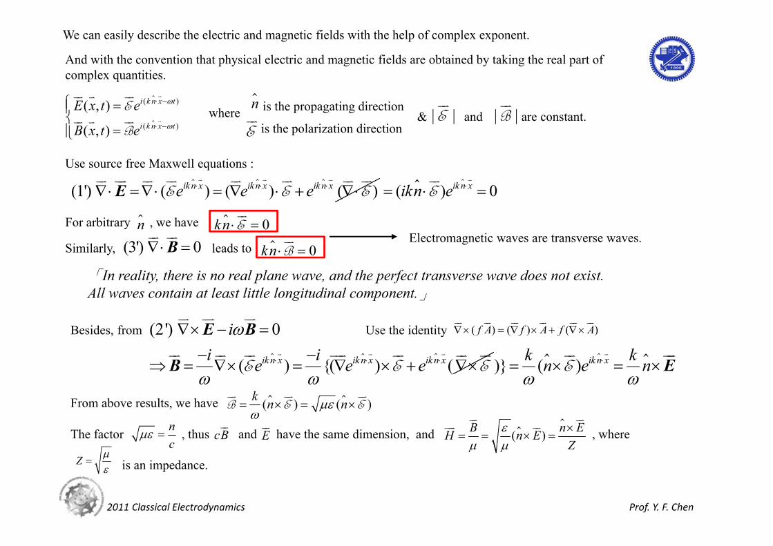
For arbitrary , we have n 0kn E
Similarly, leads to (3') 0
B 0kn B
Electromagnetic waves are transverse waves.
「In reality, there is no real plane wave, and the perfect transverse wave does not exist.All waves contain at least little longitudinal component.」
Besides, from
(2') 0
( ) {( ) (ikn x ikn x ikn x
ii ie e e
E E E
E B
B )} ( ) ikn xk kn e n
E E
( ) ( ) ( )f A f A f A
Use the identity
From above results, we have ( ) ( )k n n
B E E
The factor , thus and have the same dimension, and , where
is an impedance.
nc
cB
E
( )B n EH n EZ
Z
2011 Classical Electrodynamics Prof. Y. F. Chen
Check dimension of Z:
In ac circuits, , therefore is the dimension of inpedence. 21
cc L
L
Z L Z Z Zi cCZ i L
[ ] [ ]Z
In vacuum,7
0 12
4 10 376.7( )8.85 10
Z Z
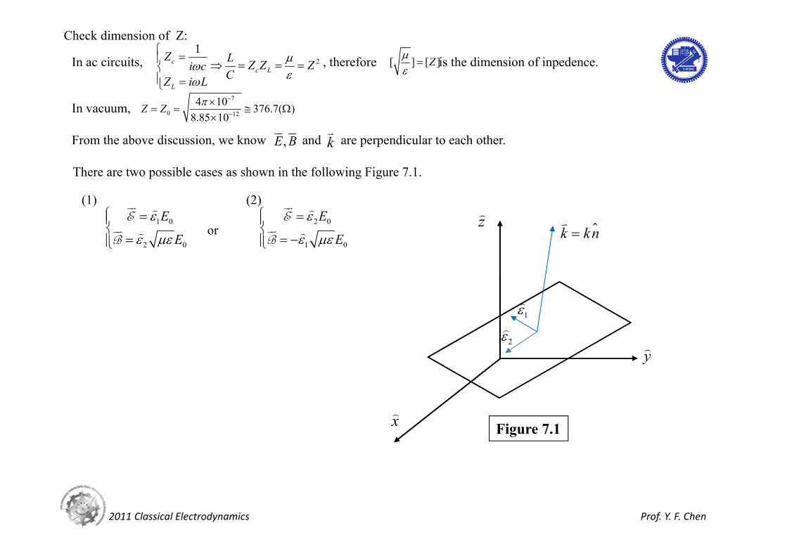
From the above discussion, we know and are perpendicular to each other. ,E B
k
There are two possible cases as shown in the following Figure 7.1.
1 0
2 0
E
E
E
Bor
(1) (2)2 0
1 0
E
E
E
B
x
y
z k kn
1
2
Figure 7.1

A First Look at Quantum Physics
2011 Classical Electrodynamics Prof. Y. F. Chen
§7.2 Linear and Circular Polarization; Stokes Parameters
We can use two orthogonal polarized-components to describe any polarized TEM wave:
x yE E i E j
and
[ ( ) ]
0 0
[ ( ) ]
0 0
cos[ ( ) ] Re( )
cos[ ( ) ] Re( )
x
y
zi tv
x x x x
zi tv
y y y y
zE E t E evzE E t E ev
where 0
0
x
y
EE
is the peak amplitude of xEis the peak amplitude of yE
Let , y x [ ( ) ]( , , ; ) [ ] x
zi ti vx yE x y z t E i E e j e
This can be represented as two components column vector:[ ( ) ]0
0
xzi tx x v
iy y
E Ee
E E e
global phase
For any fully polarized field, we can use this Maxwell column (or Jones vector) to characterize the polarized state.
For
(i) 0 or
(ii) 0 0
/ 2 & | | | |
/ 2 x yE E
(iii)
, is E left –handed circular-polarized (LCP)
right –handed circular-polarized (RCP)
Other than the above condition but is constant
, is linear-polarized (LP) E
, is elliptical-polarized E
※The general mathematical treatment for polarized light :
Let 0
0
cos( )cos( )
x x
y y
E E kz tE E kz t
0
cos( )x
x
E kz tE
0
cos( ) cos sin( )siny
y
Ekz t kz t
E
2011 Classical Electrodynamics Prof. Y. F. Chen
2 2 2 2 2 2 2
0 0
(1) ( ) ( ) cos ( ) cos ( )cos sin ( )sin 2cos( )sin( )cos sinyx
x y
EE kz t kz t kz t kz t kz tE E
2 2
0 0
(2) 2( )( ) cos 2cos ( )cos 2cos( )sin( ) cos sinyx
x y
EE kz t kz t kz tE E
2 2 2 2 2 2 2
0 0 0 0
( ) ( ) 2 cos cos ( )(1 cos ) sin ( )sin siny x yx
x y x y
E E EE kz t kz tE E E E
2 2 2
0 0 0 0
( ) ( ) 2 cos siny x yx
x y x y
E E EEE E E E
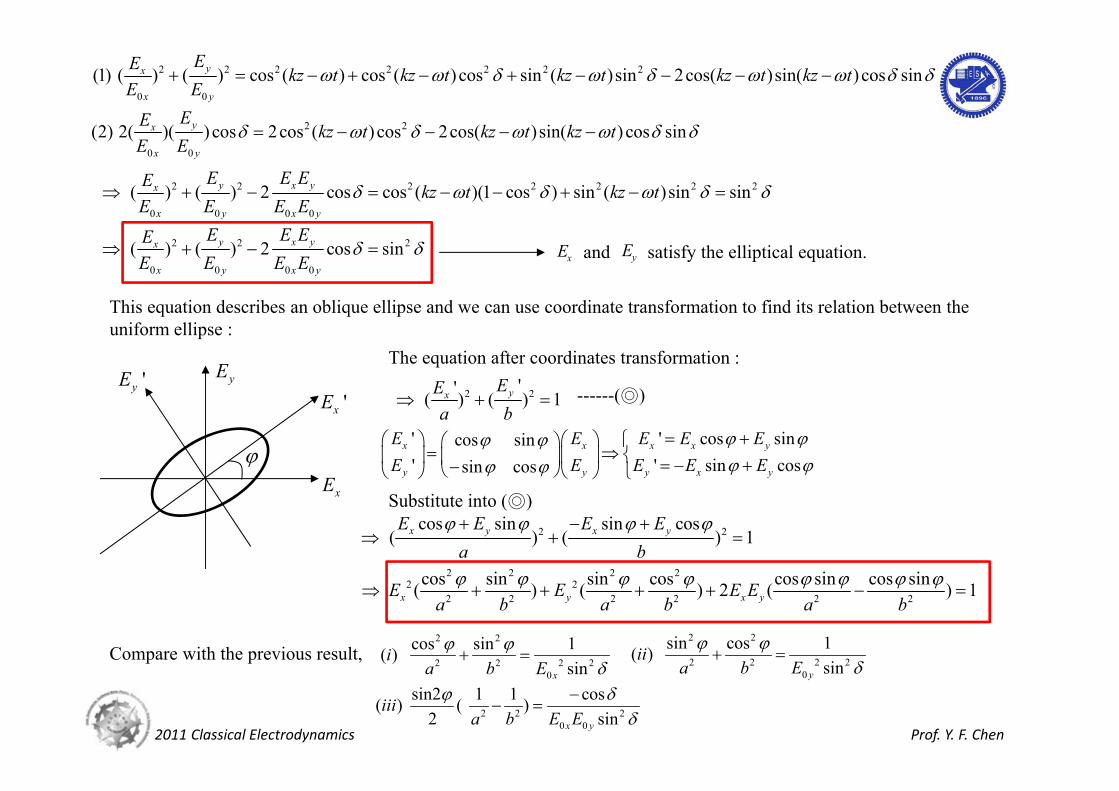
xE and satisfy the elliptical equation. yE
This equation describes an oblique ellipse and we can use coordinate transformation to find its relation between the uniform ellipse :
xE
yE'yE'xE
The equation after coordinates transformation :
2 2''( ) ( ) 1yx EEa b
' ' cos sincos sin' ' sin cossin cos
x x x x y
y y y x y
E E E E EE E E E E
------(◎)
Substitute into (◎)2 2cos sin sin cos
( ) ( ) 1x y x yE E E Ea b
2 2 2 22 2
2 2 2 2 2 2
cos sin sin cos cos sin cos sin( ) ( ) 2 ( ) 1x y x yE E E Ea b a b a b
Compare with the previous result,2 2
2 2 2 20
cos sin 1( ) sinx
ia b E
2 2
2 2 2 20
sin cos 1( ) siny
iia b E
2 2 20 0
sin2 1 1 cos( ) ( )2 sinx y
iiia b E E
2011 Classical Electrodynamics Prof. Y. F. Chen
2 2 2 2 20 0
1 1 1 1 1( ) ( ) ( ) cos 2 ( ) ( )sinx y
i ii iva b E E
Use2 2
0 0 0 02 2 2 2
0 0 0 0 0 0
2( ) 2costan 2 ( ) cos( )
x y x y
x y x y x y
E E E Eiiiiv E E E E E E
--------※
And 2 2 2 2 20 0
1 1 1 1 1( ) ( ) ( )sin x y
i iia b E E
With the fact that the area is conserved after coordinate transformation
2 22 2 2 20 0
0 0 2 2 2 2 2 2 2 20 0 0 0
( sin )( sin )sin sin
x yx y
x y x y
E Ea b a bab E Ea b E E E E
Thus, 2 2 2 20 0x ya b E E Sum of the square of the two orthogonally polarized components of elliptical polarized
states is constant.→energy conservation
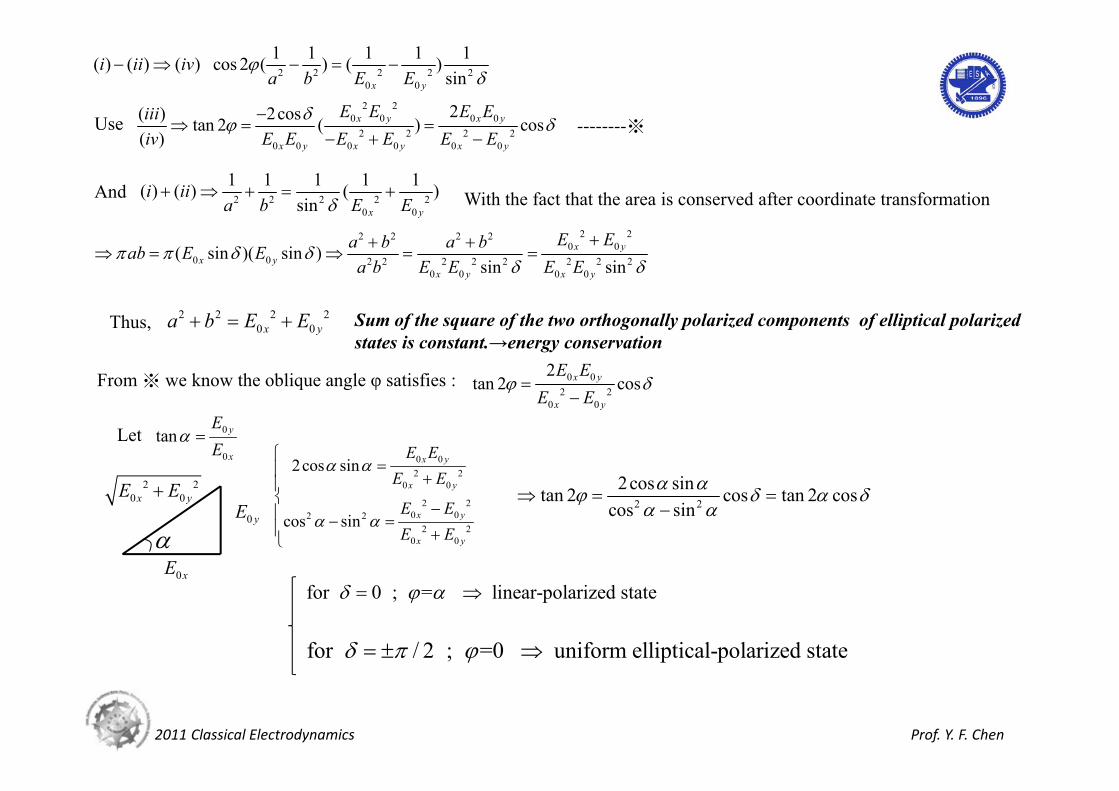
From ※ we know the oblique angle φ satisfies : 0 02 2
0 0
2tan 2 cosx y
x y
E EE E
Let 0
0
tan y
x
EE
0 yE
0xE
2 20 0x yE E
0 02 2
0 0
2 20 02 2
2 20 0
2cos sin
cos sin
x y
x y
x y
x y
E EE E
E EE E
2 2
2cos sintan 2 cos tan 2 coscos sin
for 0 ; = linear-polarized state
for / 2 ; =0 uniform elliptical-polarized state
2011 Classical Electrodynamics Prof. Y. F. Chen
“Some of the types of light that fall between the fully coherent and fully incoherentextremes are called partially polarized light.”
One can create partially polarized light by starting with a laser. In some scientific experiments, the complete coherent of a laser beam can be an embarrassment because of the unwanted effects of interference or diffraction or “speckle” that it produce.
Quasi-thermal light is manufactured by sending a laser beam through a coherent-degrading device, such as a rapidly rotating ground-glass (or diffuser).
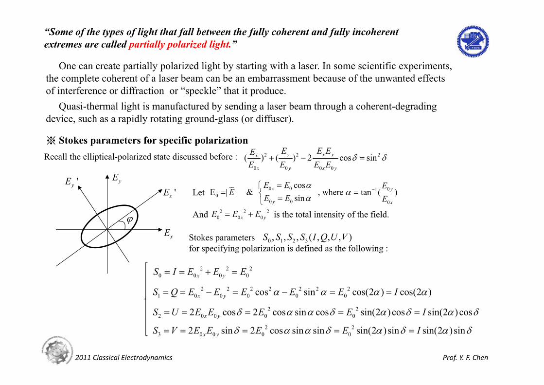
※ Stokes parameters for specific polarizationRecall the elliptical-polarized state discussed before : 2 2 2
0 0 0 0
( ) ( ) 2 cos siny x yx
x y x y
E E EEE E E E
xE
yE'yE'xE
Let 0 0 010
0 0 0
cosE | | & , where tan ( )
sinx y
y x
E E EE
E E E
And is the total intensity of the field. 2 2 20 0 0x yE E E
Stokes parameters for specifying polarization is defined as the following :
0 1 2 3, , , ( , , , )S S S S I Q U V
2 2 20 0 0 0x yS I E E E
2 2 2 2 2 2 21 0 0 0 0 0cos sin cos(2 ) cos(2 )x yS Q E E E E E I
2 22 0 0 0 02 cos 2 cos sin cos sin(2 )cos sin(2 )cosx yS U E E E E I
2 23 0 0 0 02 sin 2 cos sin sin sin(2 )sin sin(2 )sinx yS V E E E E I

2011 Classical Electrodynamics Prof. Y. F. Chen
All these parameters form a three-dimensional sphere :
1S
2S
3S
2
Figure 7.2.1 Poincarѐ sphere
2 2 2 2 2 2 2 20 1 2 3 ( )S S S S I Q U V
The degree of polarization is defined as:
2 2 2
2 , 0 1Q U VP PI
If random polarized, then 0Q U V
For a beam that is partially polarized, we define a “degree of polarization” P, which is equal to the positive square root of the ratio .
2 2 2
2
Q U VI
One can use proper optical elements like polarizer and wave-plate to measure all the Stokes parameters.
Assume the Jones vector for the incident field is 0
0
xi
y
EE e
Step1: incident on a polarizer with horizontal transmitting axis 0 0 21 0
0
1 00 0 0
x xi x
y
E EI E
E e
Step2: incident on a polarizer with vertical transmitting axis 0 22 0
0 0
00 00 1
xi i y
y y
EI E
E e E e
1 2 0
1 2 1
I I SI I S
2011 Classical Electrodynamics Prof. Y. F. Chen
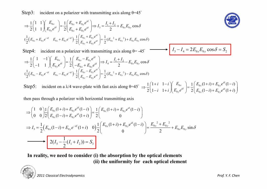
Step3: incident on a polarizer with transmitting axis along θ=45°
0 0 0 1 23 0 0
0 0 0
1 11 1 cos1 12 2 2
ix x yi x yi
y x y
E E E e I II E EE e E E e
0 0 2 20 0 0 0 0 0 0 0
0 0
1 1 1( ( ) cos )2 2 2
ix yi i
x y x y x y x yix y
E E eE E e E E e E E E E
E E e
Step4: incident on a polarizer with transmitting axis along θ= -45°
0 0 0 1 24 0 0
0 0 0
1 11 1 cos1 12 2 2
ix x yi x yi
y x y
E E E e I II E EE e E E e
0 0 2 20 0 0 0 0 0 0 0
0 0
1 1 1( ( ) cos )2 2 2
ix yi i
x y x y x y x yix y
E E eE E e E E e E E E E
E E e
3 4 0 0 22 cosx yI I E E S
Step5: incident on a λ/4 wave-plate with fast axis along θ=45° 0 0 0
0 0 0
(1 ) (1 )1 11 1(1 ) (1 )1 12 2
ix x yi i
y x y
E E i E e ii iE e E i E e ii i
then pass through a polarizer with horizontal transmitting axis
0 0 0 0
0 0
(1 ) (1 )1 0 (1 ) (1 )1 1(1 ) (1 )0 0 2 2 0
i ix y x y
ix y
E i E e i E i E e iE i E e i
2 2
0 00 05 0 0 0 0
(1 ) (1 )1 1(1 ) (1 ) 0 sin2 2 20
ix yi x y
x y x y
E EE i E e iI E i E e i E E
5 1 2 312( ( ))2
I I I S
In reality, we need to consider (i) the absorption by the optical elements(ii) the uniformity for each optical element
2011 Classical Electrodynamics Prof. Y. F. Chen
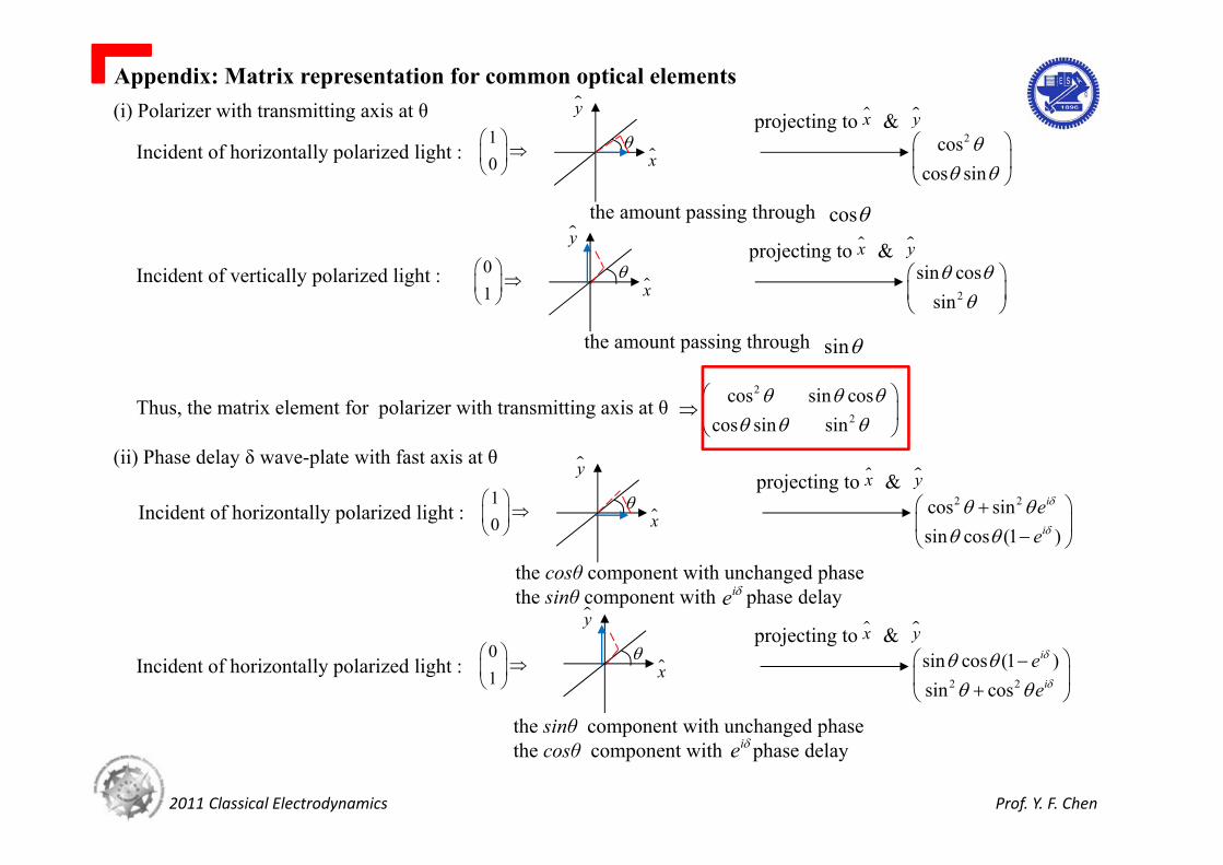
Appendix: Matrix representation for common optical elements(i) Polarizer with transmitting axis at θ
Incident of horizontally polarized light : 10
x
y
the amount passing through cos
projecting to & x y2cos
cos sin
Incident of vertically polarized light : 01
x
y
the amount passing through sin
projecting to & x y
2
sin cossin
Thus, the matrix element for polarizer with transmitting axis at θ2
2
cos sin coscos sin sin
(ii) Phase delay δ wave-plate with fast axis at θ
Incident of horizontally polarized light : 10
x
y
the cosθ component with unchanged phasethe sinθ component with phase delay
projecting to & x y
ie
2 2cos sinsin cos (1 )
i
i
ee
Incident of horizontally polarized light : 01
the sinθ component with unchanged phasethe cosθ component with phase delay
projecting to & x y
ie
2 2
sin cos (1 )sin cos
i
i
ee
x
y
2011 Classical Electrodynamics Prof. Y. F. Chen
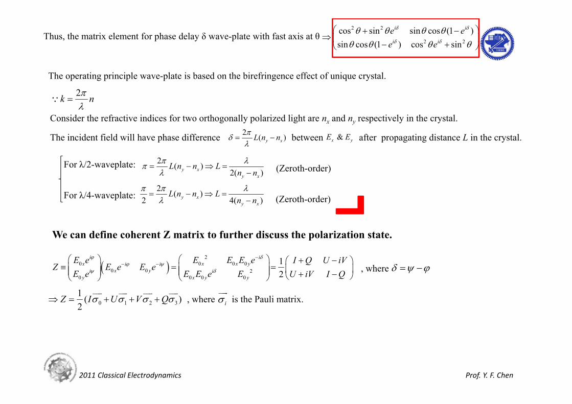
Thus, the matrix element for phase delay δ wave-plate with fast axis at θ2 2
2 2
cos sin sin cos (1 )sin cos (1 ) cos sin
i i
i i
e ee e
The operating principle wave-plate is based on the birefringence effect of unique crystal.
2
k n
Consider the refractive indices for two orthogonally polarized light are nx and ny respectively in the crystal.
The incident field will have phase difference between after propagating distance L in the crystal.2 ( )
y xL n n & x yE E
For λ/2-waveplate: 2 ( )2( )
y x
y x
L n n Ln n (Zeroth-order)
For λ/4-waveplate: 2 ( )
2 4( )
y xy x
L n n Ln n (Zeroth-order)
We can define coherent Z matrix to further discuss the polarization state.
2
0 0 0 00 0 2
0 0 0 0
12
i ix x x yi i
x yi iy x y y
E e E E E e I Q U iVZ E e E e
E e E E e E U iV I Q , where
0 1 2 31 ( )2
Z I U V Q , where is the Pauli matrix.
i
2011 Classical Electrodynamics Prof. Y. F. Chen
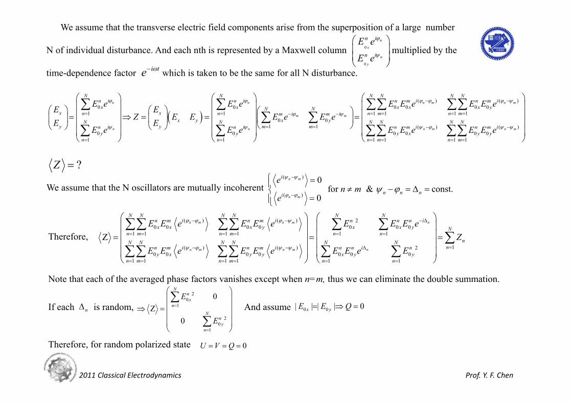
We assume that the transverse electric field components arise from the superposition of a large number
N of individual disturbance. And each nth is represented by a Maxwell column multiplied by the
time-dependence factor which is taken to be the same for all N disturbance.
0
0
n
x
n
y
in
in
E e
E ei te
( ) ( )
0 0 0 0 0 01 1 1 1 1 1
0 01 1
0 0 0 01 1
n n n m n m
m m
n n
N N N N N Ni i i in n n m n m
x x x x x yN Nx xn n n m n mi im m
x y x yN Ny y m mi in n n
y y yn n
E e E e E E e E E eE EZ E E E e E e
E EE e E e E E ( ) ( )
0 01 1 1 1
n m n m
N N N Ni im n m
x y yn m n m
e E E e
?Z
We assume that the N oscillators are mutually incoherent( )
( )
0 for & const.
0
n m
n m
i
n n ni
en m
e
Therefore,
( ) ( ) 20 0 0 0 0 0 0
1 1 1 1 1 1
1( ) ( ) 20 0 0 0 0 0 0
1 1 1 1 1 1
Z
n m n m n
n m n m n
N N N N N Ni i in m n m n n n
x x x y x x y Nn m n m n n
nN N N N N Nni i in m n m n n n
y x y y x y yn m n m n n
E E e E E e E E E eZ
E E e E E e E E e E
Note that each of the averaged phase factors vanishes except when n=m, thus we can eliminate the double summation.
If each is random, n
20
1
20
1
0Z
0
Nnx
nN
ny
n
E
EAnd assume 0 0| | | | 0 x yE E Q
Therefore, for random polarized state 0 U V Q
A First Look at Quantum Physics
2011 Classical Electrodynamics Prof. Y. F. Chen
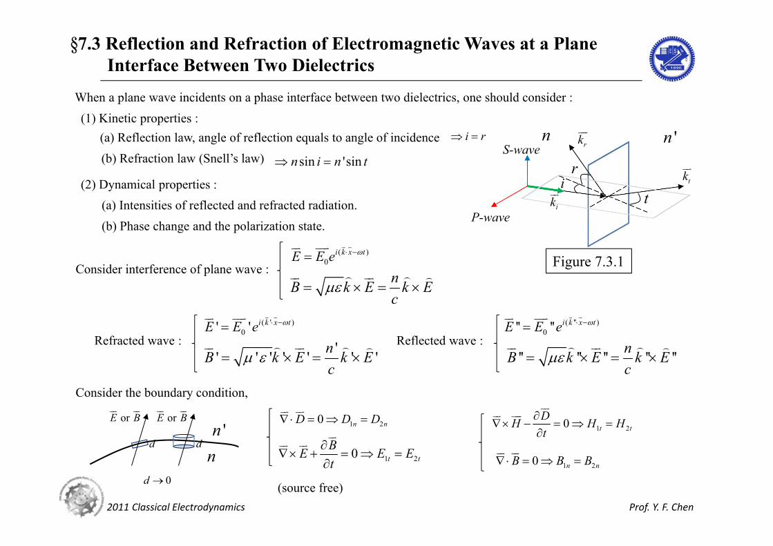
§7.3 Reflection and Refraction of Electromagnetic Waves at a Plane Interface Between Two Dielectrics
When a plane wave incidents on a phase interface between two dielectrics, one should consider :(1) Kinetic properties :
(a) Reflection law, angle of reflection equals to angle of incidence i r
(b) Refraction law (Snell’s law) sin 'sinn i n t
(2) Dynamical properties :(a) Intensities of reflected and refracted radiation.(b) Phase change and the polarization state.
ir
tP-wave
S-wave
ik
rk
tk
n 'n
Figure 7.3.1Consider interference of plane wave :( )
0i k x tE E e
nB k E k Ec
Refracted wave :( ' )
0' ' i k x tE E e
'' ' ' ' ' ' 'nB k E k Ec
Reflected wave :
( '' )0'' '' i k x tE E e
'' '' '' '' ''nB k E k Ec
Consider the boundary condition,
n'n
dd
0d
or E B
or E B
1 20 n nD D D
1 20 t tBE E Et
(source free)
1 20 n nB B B
1 20 t tDH H Ht
2011 Classical Electrodynamics Prof. Y. F. Chen
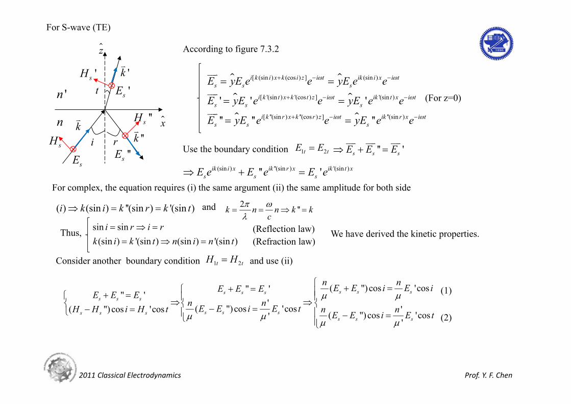
For S-wave (TE)
n
'n
k
''k
'k
i r
t
sE ''sE
'sE
sH
''sH
'sH
x
z According to figure 7.3.2
[ (sin ) (cos ) ] (sin )
[ '(sin ) '(cos ) ] '(sin )
[ ''(sin ) ''(cos ) ] ''(sin )
' ' '
'' '' ''
i k i x k i z i t ik i x i ts s s
i k t x k t z i t ik t x i ts s s
i k r x k r z i t ik r x i ts s s
E yE e e yE e e
E yE e e yE e e
E yE e e yE e e
(For z=0)
Use the boundary condition 1 2t tE E '' 's s sE E E
(sin ) ''(sin ) '(sin )'' 'ik i x ik r x ik t xs s sE e E e E e
For complex, the equation requires (i) the same argument (ii) the same amplitude for both side
( ) (sin ) ''(sin ) '(sin )i k i k r k t and 2 ''k n n k kc
sin sin(sin ) '(sin ) (sin ) '(sin )
i r i rk i k t n i n t
Thus, (Reflection law)(Refraction law)
We have derived the kinetic properties.
Consider another boundary condition and use (ii) 1 2t tH H
( ")cos 'cos" '" '
'( ")cos 'cos( ") cos 'cos '( ")cos 'cos''
s s ss s ss s s
s s ss s ss s s
n nE E i E iE E EE E E
n nE E i E tH H i H t n nE E i E t
(1)
(2)
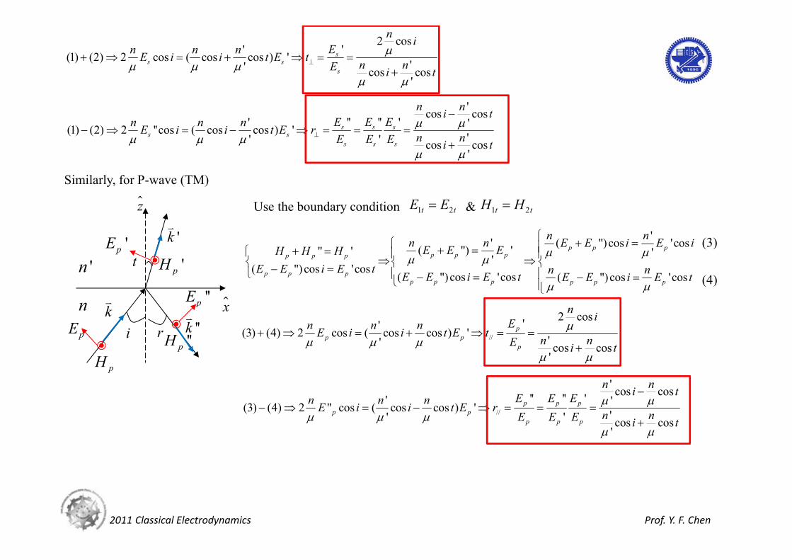
2011 Classical Electrodynamics Prof. Y. F. Chen
2 cos''(1) (2) 2 cos ( cos cos ) ' '' cos cos
'
ss s
s
n iEn n nE i i t E t n nE i t
'cos cos'' '' '' '(1) (2) 2 ''cos ( cos cos ) ' '' ' cos cos
'
s s ss s
s s s
n ni tE E En n nE i i t E r n nE E E i t
Similarly, for P-wave (TM)
n
'n
k
''k
'k
i r
t
pE
''pE
'pE
pH''pH
'pH
x
z Use the boundary condition & 1 2t tE E 1 2t tH H
'' ( ") cos 'cos( ") '" ' ''( ") cos 'cos
( ")cos 'cos ( ")cos 'cos
p p pp p pp p p
p p pp p p p p p
n nn n E E i E iE E EH H HE E i E t n nE E i E t E E i E t
(3)
(4)
//
2 cos''(3) (4) 2 cos ( cos cos ) ' '' cos cos'
pp p
p
n iEn n nE i i t E t n nE i t
//
' cos cos'' '' '' '(3) (4) 2 " cos ( cos cos ) ' '' ' cos cos'
p p pp p
p p p
n ni tE E En n nE i i t E r n nE E E i t
2011 Classical Electrodynamics Prof. Y. F. Chen
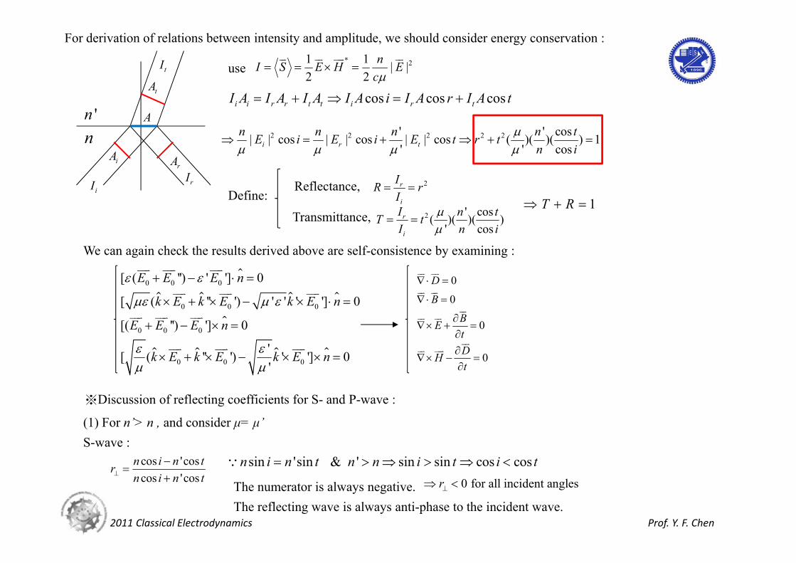
For derivation of relations between intensity and amplitude, we should consider energy conservation :
n'n A
iA
tA
rA
iI rI
tI
cos cos cosi i r r t t i r tI A I A I A I A i I A r I A t
use* 21 1 | |
2 2nI S E H E
c
2 2 2 2 2' ' cos| | cos | | cos | | cos ( )( )( ) 1' ' cosi r t
n n n n tE i E i E t r tn i
Define: Reflectance, 2r
i
IR rI
Transmittance, 2 ' cos( )( )( )' cos
r
i
I n tT tI n i
1T R
We can again check the results derived above are self-consistence by examining :
0 0 0
0 0 0
0 0 0
0 0 0
[ ( '') ' '] 0
[ ( '' ') ' ' ' '] 0
[( '') '] 0
'[ ( '' ') ' '] 0'
E E E n
k E k E k E n
E E E n
k E k E k E n
0
0
0
0
D
B
BEtDHt
※Discussion of reflecting coefficients for S- and P-wave :
(1) For n’> n , and consider μ= μ’
cos 'coscos 'cos
n i n trn i n t
sin 'sin & ' sin sin cos cosn i n t n n i t i t
The numerator is always negative. 0 for all incident anglesr
The reflecting wave is always anti-phase to the incident wave.
S-wave :
2011 Classical Electrodynamics Prof. Y. F. Chen
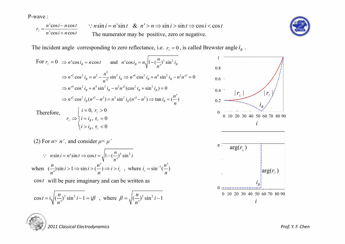
P-wave :
//'cos cos'cos cos
n i n trn i n t
sin 'sin & ' sin sin cos cosn i n t n n i t i t
The numerator may be positive, zero or negative.
The incident angle corresponding to zero reflectance, i.e. , is called Brewster angle .// 0r Bi
For // 0r 2 2
42 2 2 2 4 2 4 2 2 2
2
4 2 4 2 2 2 2 2
2 2 2 2 2 2 2 2
'cos cos and 'cos 1 ( ) sin'
' cos sin ' cos sin ' 0'
' cos sin ' (cos sin ) 0'' cos ( ' ) sin ( ' ) tan ( )
B B B
B B B B
B B B B
B B B
nn i n t n i n in
nn i n i n i n i n nn
n i n i n n i inn i n n n i n n in
Therefore, //
// //
//
0, 0, r 0, r 0
B
B
i rr i i
i i
0 10 20 30 40 50 60 70 80 90
Bi
i
0
0.2
0.4
0.6
0.8
1
//| |r| |r
0 10 20 30 40 50 60 70 80 90
Bi
i
//arg( )r
arg( )r
0
π(2) For n> n’ , and consider μ= μ’
2 2 sin 'sin cos 1 ( ) sin'
nn i n t t in
when 1' '( ) sin 1 sin ( ) , where sin ( )' c c
n n ni i i i in n n
will be pure imaginary and can be written ascos t
2 2 2 2cos i ( ) sin 1 i , where ( ) sin 1' '
n nt i in n
A First Look at Quantum Physics
2011 Classical Electrodynamics Prof. Y. F. Chen
§7.4 Polarization by Reflection , Total Internal Reflection;Goos-Hänchen Effect
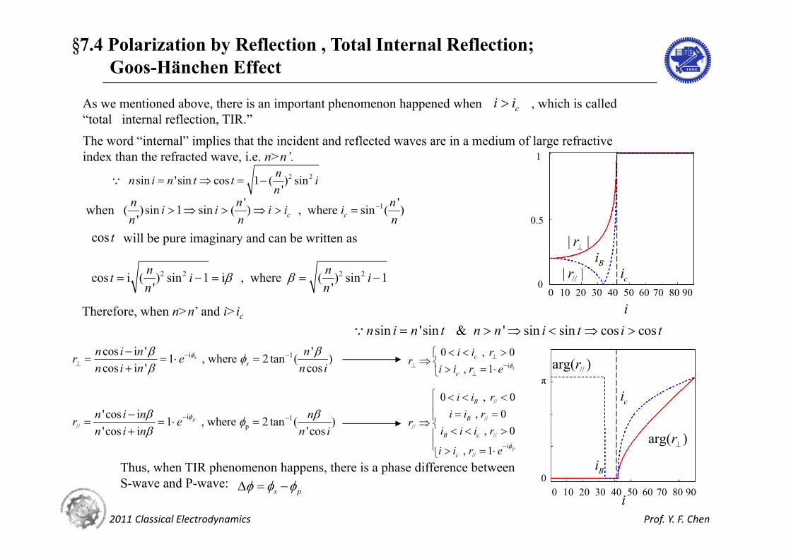
As we mentioned above, there is an important phenomenon happened when , which is called “total internal reflection, TIR.”
ci i
The word “internal” implies that the incident and reflected waves are in a medium of large refractive index than the refracted wave, i.e. n>n’.
2 2 sin 'sin cos 1 ( ) sin'
nn i n t t in
when 1' '( )sin 1 sin ( ) , where sin ( )' c c
n n ni i i i in n n
will be pure imaginary and can be written ascos t
2 2 2 2cos i ( ) sin 1 i , where ( ) sin 1' '
n nt i in n
Therefore, when n>n’ and i>ic
si 1cos i ' '1 , where 2 tan ( )cos i ' coss
n i n nr en i n n i
i 1// p
'cos i 1 , where 2 tan ( )'cos i 'cos
pn i n nr en i n n i
sin 'sin & ' sin sin cos cosn i n t n n i t i t
i
0 , 0 , 1 s
c
c
i i rr
i i r e
//
////
//
i//
0 , 0, 0
, 0
, 1 p
B
B
B c
c
i i ri i r
ri i i r
i i r e
0 10 20 30 40 50 60 70 80 90
i
Bi//| |r
| |r
ci0
0.5
1
0 10 20 30 40 50 60 70 80 90i
//arg( )r
arg( )r
Bi
ci
0
π
Thus, when TIR phenomenon happens, there is a phase difference between S-wave and P-wave:
s p
2011 Classical Electrodynamics Prof. Y. F. Chen
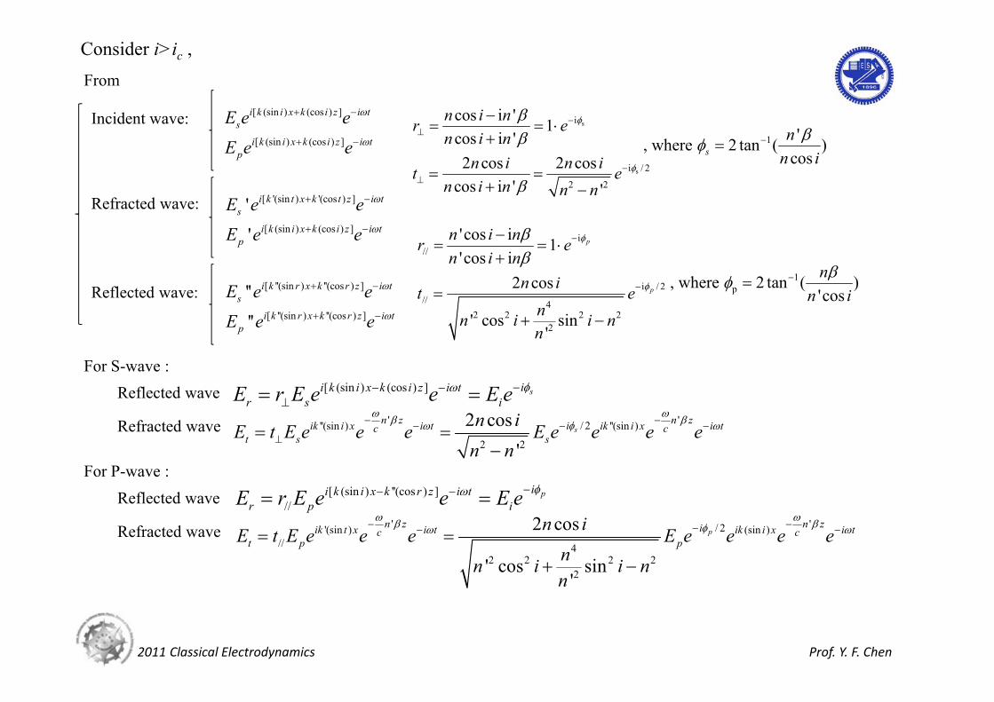
Consider i>ic , From
Incident wave: [ (sin ) (cos ) ]
[ (sin ) (cos ) ]
i k i x k i z i ts
i k i x k i z i tp
E e e
E e e
Refracted wave: [ '(sin ) '(cos ) ]
[ (sin ) (cos ) ]
'
'
i k t x k t z i ts
i k i x k i z i tp
E e e
E e e
[ ''(sin ) ''(cos ) ]
[ ''(sin ) ''(cos ) ]
''
''
i k r x k r z i ts
i k r x k r z i tp
E e e
E e e
Reflected wave:
s
s
i
i / 2
2 2
cos i ' 1cos i '2 cos 2 cos
cos i ' '
n i nr en i n
n i n it en i n n n
i//
i / 2// 4
2 2 2 22
'cos i 1'cos i
2 cos
' cos sin'
p
p
n i nr en i n
n it enn i i nn
1 ', where 2 tan ( )cossn
n i
1p, where 2 tan ( )
'cosn
n i
For S-wave : Reflected wave [ (sin ) (cos ) ] sii k i x k i z i t
r s iE r E e e E e
Refracted wave ' '/ 2''(sin ) ''(sin )
2 2
2 cos'
sn z n ziik i x i t ik i x i tc c
t s sn iE t E e e e E e e e e
n n
For P-wave :
Reflected wave
Refracted wave
[ (sin ) ''(cos ) ]//
pii k i x k r z i tr p iE r E e e E e
' '/ 2'(sin ) (sin )// 4
2 2 2 22
2 cos
' cos sin'
pn z n ziik t x i t ik i x i tc c
t p pn iE t E e e e E e e e e
nn i i nn
2011 Classical Electrodynamics Prof. Y. F. Chen
According to above results, when i>ic , all the reflected waves for S- & P-wave will experience an additional phase shift and , which changes the original polarized state.s p
Consider, the incident wave with original polarized state 0
0
xi
y
EE e
0( )
0
s
p
ix
iy
E e
E e
after reflection
assume x s
y p
E EE E
Furthermore, although the reflecting coefficient equals to 1, the refracted wave can penetrate certain depth along the z-axis.
dZ
'dczn
(for monochromatic wave)If 2 2 1' 1 & 1.5 , 45 ( ) sin 1
' 2 2nn n i in
14 82 10 (Hz) ; 3 10 ( / )c m s
61.3506 10 ( ) ~dz m m
The refracted wave is propagated only parallel to the surface and is attenuated exponentially beyond the interface.
Even though fields exist on the other side of the interface, there is no energy net energy flow through the interface.The phenomenon is called evanescent wave.
We can calculate the time-averaged normal component of the Poynting vector just inside the surface :
*
20
1 ( ' ')Re[ ( ' ' )] with '2 '
1 Re[( ') | ' | ]2 '
k ES n n E H H
S n n k E
and ' 'cos is pure imaginary 0 (no net energy flow)n k k t S n
A First Look at Quantum Physics
2011 Classical Electrodynamics Prof. Y. F. Chen
§7.5 Frequency Dispersion Characteristics of Dielectrics,Conductors, and Plasmas
“In reality, all media show some dispersion.” (Unless we consider a limited range of frequencies.)
0
( )( ) , for non-magnetic material 1 ( ) ( )( ) ( ) r r
r r
c cv nn
A. Simple Model for ( ) Recall (4.69), if we consider the difference between local field and applied field : 11
3
mole
mol
N
N
If we neglect the difference between local and applied field : e molN
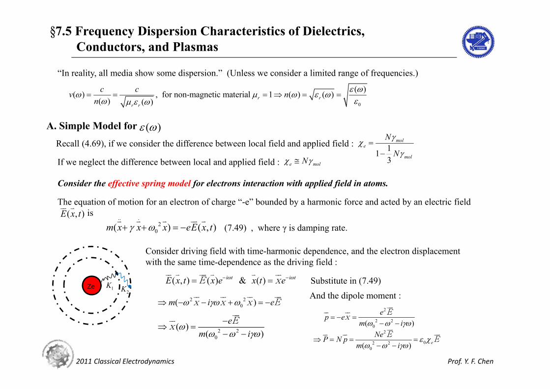
Consider the effective spring model for electrons interaction with applied field in atoms.
The equation of motion for an electron of charge “-e” bounded by a harmonic force and acted by an electric fieldis ( , )E x t
.. .
20( ) ( , )m x x x eE x t
(7.49) , where γ is damping rate.
Ze 1K2K
Consider driving field with time-harmonic dependence, and the electron displacement with the same time-dependence as the driving field :
( , ) ( ) & ( )i t i tE x t x e x t e
E x Substitute in (7.49)
2 20( )m i e
x x x E
2 20
( )( )
em i
Ex
And the dipole moment :2
2 20( )
ep em i
Ex
2
02 20( ) e
NeP N pm i
EE
2011 Classical Electrodynamics Prof. Y. F. Chen
Recall :0
0
0 0 0 0 0
& ( )
(1 ) (1 )
f pp f f
e e e
P P
P
E E D
D E E E E E
Therefore, we have2
2 20 0( )e
Nem i
Suppose that there are N molecules per unit volume with Z electrons per molecule and that instead of a single binding frequency for all, there are fj electrons per molecule with binding frequency ωj and damping constant ϒj , then the dielectric constant, , is given by 0/ 1 e
2
2 20 0
( ) 1( )
j
j j j
fNem i
(7.51)
, where the oscillator strength fj satisfy the sum rule : jj
f Z (7.52) (Electric charge conservation)
With subtle quantum-mechanical definition of fj , ωj ,ϒj (7.51) is an accurate description of the atomic contribution to the dielectric constant.
In Q.M. , we can calculate the probability of transition between two levels induced by the interaction potential V to find out ωj ,ϒj .
According to Fermi-Gorden rule : 2 ( )i ff i i f
PV E E
Also, we can decide the generalized oscillator strength (GOS) fj , by evaluating 2| |f i x
(Assuming the applied field are not too strong to effect the wave function.)

2011 Classical Electrodynamics Prof. Y. F. Chen
In general solid state physics,j
if consider valence (outer) shell electrons, if consider inner shell electrons,
j g
g
EE
One can classify different types of atoms by checking the behavior of inner shell electrons.By fitting the experimental data, one can obtain parameters fj , ωj ,ϒj to construct an empirical model.
B. Anomalous Dispersion and Resonant Absorption
In general case, j j If 2 2 1
2 2 1
, the factor ( ) is positive, the factor ( ) is negative
j j j
j j j
At low frequency, below the smallest all the terms in the sum contribute with the samepositive sign, and greater than unity.
j2 2( )
j
j j j
fi
( )
“Normal dispersion is associated with an increase in with ω, anomalous disperse with the inverse.” Re( )
From the mathematical form we know that every time when it would be positive imaginary,
and from to the sign will be inverse one time.
2 2
1
j ji j
j j
0
( )Re( )
0
( )Im( )
1310 1410( )Hz
Since a positive imaginary part to ε represents dissipation of energy from the EM wave into the medium, the region where Im(ε) is large are called “the region of resonant dissipation.”
1
2 3
4 5
Recall :
0 0
( )kc
, the imaginary part of ε(ω) may let the wave number be written as
2011 Classical Electrodynamics Prof. Y. F. Chen
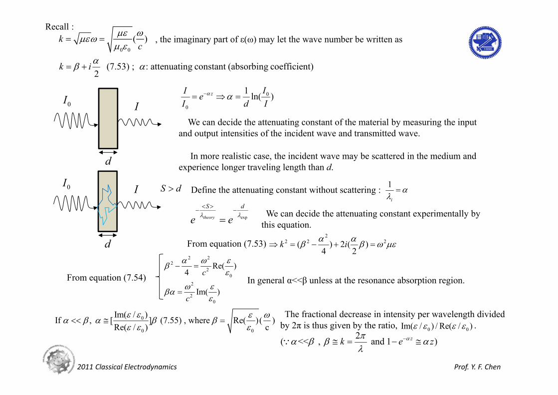
(7.53) ; : attenuating constant (absorbing coefficient)2
k i
0I I
d
0
0
1 ln( )z II eI d I
We can decide the attenuating constant of the material by measuring the input and output intensities of the incident wave and transmitted wave.
In more realistic case, the incident wave may be scattered in the medium and experience longer traveling length than d.
0I I
d
S d Define the attenuating constant without scattering : 1
i
exptheory
S d
e e
We can decide the attenuating constant experimentally by this equation.
From equation (7.53)2
2 2 2( ) 2 ( )4 2
k i
From equation (7.54)
2 22
20
2
20
Re( )4
Im( )
c
c
In general α<<β unless at the resonance absorption region.
0
0 0
Im( / )If , [ ] (7.55) , where Re( )( ) Re( / ) c
The fractional decrease in intensity per wavelength divided
by 2π is thus given by the ratio, . 0 0Im( / ) / Re( / ) 2( << , and 1 )zk e z
2011 Classical Electrodynamics Prof. Y. F. Chen
C. Low-frequency Behavior, Electric Conductivity
In the limit ω→0, there is a qualitative difference in the response of the medium depending on whether the lowest resonant frequency is zero (conductor) or non-zero (insulator).
For ω=0, some fraction f0 of the electrons per molecule are “free” , and the dielectric constant is singular at ω=0 .
Consider the contribution of the free electrons is exhibited separated, 2
00
0
(7.51) ( ) ( ) (7.56)( )bNe fi
m i
contribution of all the other dipoles
By checking ; bDJ D Et
H Assume the medium obeys Ohm’s law , and has a “normal”
dielectric constant . J E
b
Under time-harmonic assumption, ( )bii E
H
We can think off all the contribution from the dielectric function : ( )i E H
By comparison, we know2
0
0( )Ne f
m i
For ω=0 2
00 0
0
1, and (electron density) , where is the momentum relaxation time.Ne f Nf nm
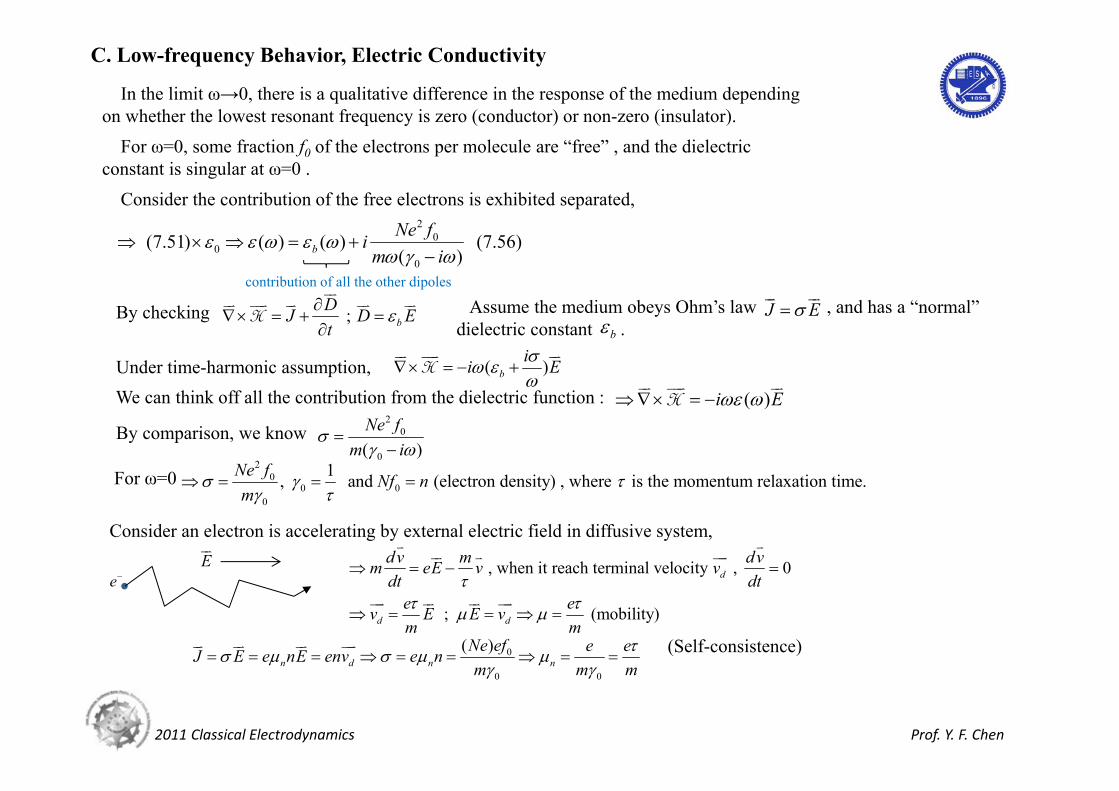
Consider an electron is accelerating by external electric field in diffusive system,
eE
, when it reach terminal velocity , 0
; (mobility)
d
d d
dv m dvm eE v vdt dt
e ev E E vm m
0
0 0
( )n d n n
Ne ef e eJ E e nE env e nm m m
(Self-consistence)
For copper (Cu), and low-frequency
2011 Classical Electrodynamics Prof. Y. F. Chen
283
#8 10 ( )Nm
7 15.9 10 ( )m 1 13 10
0
( ) 4 10 ( )f s
assume f0 =1 , then up to frequencies well beyond the microwave region conductivities of metals are essentially real (current in-phase with the field) and independent of frequency.
11 110 ( )s
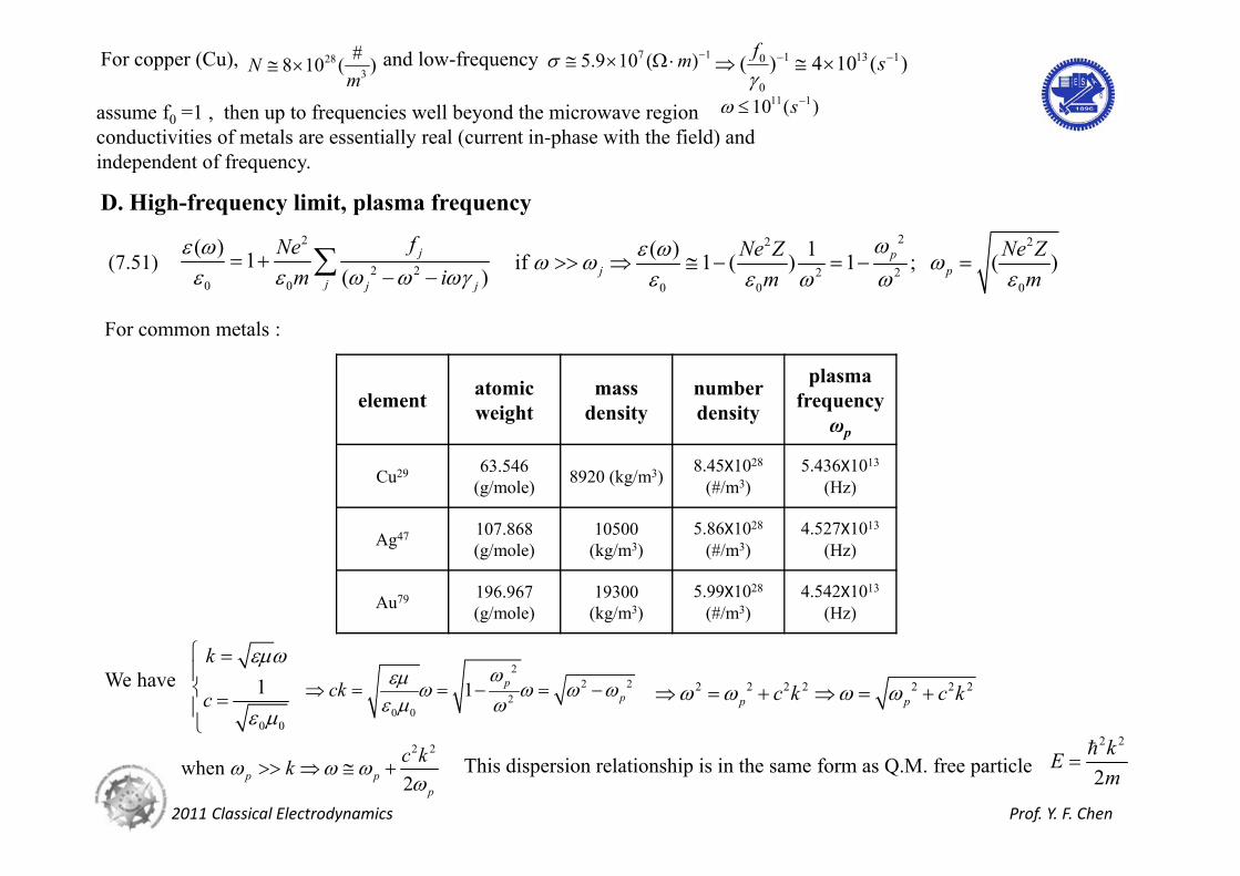
D. High-frequency limit, plasma frequency2
2 20 0
( ) 1( )
j
j j j
fNem i
(7.51)
22 2
2 20 0 0
( ) 1if 1 ( ) 1 ; ( )pj p
Ne Z Ne Zm m
For common metals :
element atomic weight
mass density
numberdensity
plasma frequency
ωp
Cu29 63.546 (g/mole) 8920 (kg/m3) 8.45X1028
(#/m3)5.436X1013
(Hz)
Ag47 107.868 (g/mole)
10500 (kg/m3)
5.86X1028
(#/m3)4.527X1013
(Hz)
Au79 196.967 (g/mole)
19300 (kg/m3)
5.99X1028
(#/m3)4.542X1013
(Hz)
We have
0 0
1k
c
22 2
20 0
1 ppck
2 2 2 2 2 2 2p pc k c k
2 2
when 2p p
p
c kk
This dispersion relationship is in the same form as Q.M. free particle 2 2
2kEm
2011 Classical Electrodynamics Prof. Y. F. Chen
holds over a wide range of frequencies including ω<ωp for a tenuous
electronic plasma in the laboratory scale.
On the laboratory scale, plasma densities are of the order of 1018 -1022 electrons m3 .
This means
2
20
( ) 1 p
10 126 10 ~ 6 10 ( )p Hz 2
2 2 2 2p 2
1When < (pure imaginary) (1 )2
pp p
p
ick k
c c
for pp
ik
c
2Compare with
2p
effk ic
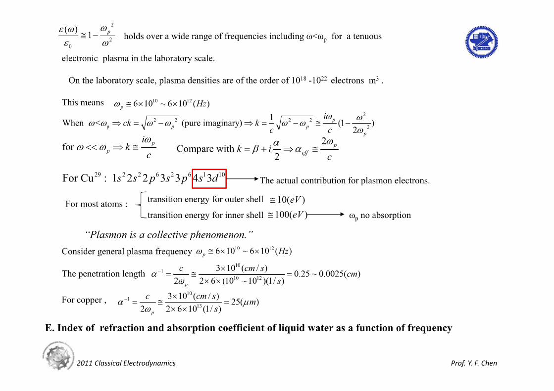
29 2 2 6 2 6 1 10For Cu : 1 2 2 3 3 4 3s s p s p s d The actual contribution for plasmon electrons.
For most atoms : transition energy for outer shell 10( )eV
transition energy for inner shell 100( )eV ωp no absorption
“Plasmon is a collective phenomenon.”Consider general plasma frequency 10 126 10 ~ 6 10 ( )p Hz
The penetration length 10
110 12
3 10 ( / ) 0.25 ~ 0.0025( )2 2 6 (10 ~ 10 )(1/ )p
c cm s cms
For copper ,10
113
3 10 ( / ) 25( )2 2 6 10 (1/ )p
c cm s ms
E. Index of refraction and absorption coefficient of liquid water as a function of frequency

2011 Classical Electrodynamics Prof. Y. F. Chen
0 0
( ) Re( )
( ) 2 Im( )
n
(Recall) 22 2
k i n i
2 2 20If , ( ) ( ) and ( ) ( ) (2 )r in n i i n i n i n
“In more general case, the dielectric function may depend on both the wave number and frequency.”
“Linhard theory is a quantum mechanical treatment for the dielectric function, which is based on the perturbation theory. “
( , )k
§7.6 Simplified Model of Propagation in the Ionosphere and MagnetosphereA First Look at Quantum Physics
2011 Classical Electrodynamics Prof. Y. F. Chen
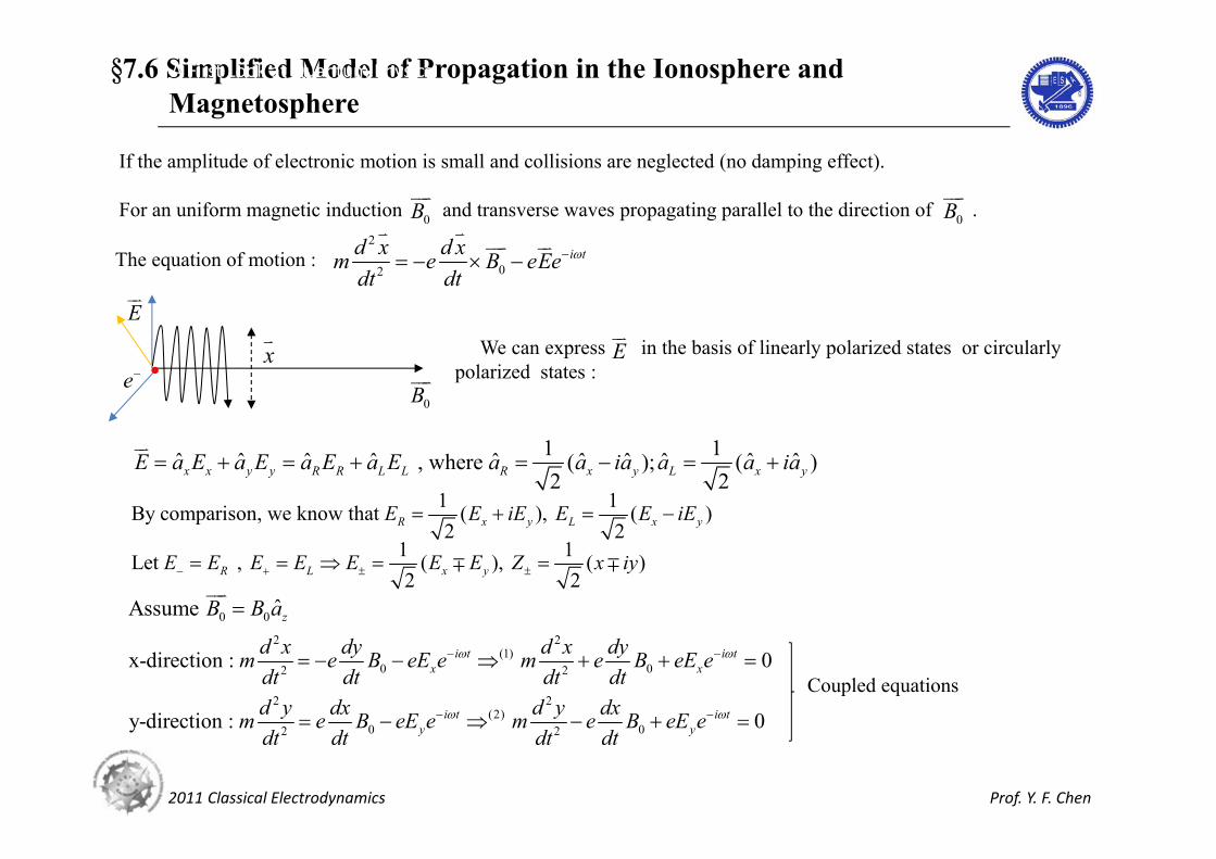
If the amplitude of electronic motion is small and collisions are neglected (no damping effect).
For an uniform magnetic induction and transverse waves propagating parallel to the direction of . 0B
0B
The equation of motion : 2
02i td x d xm e B eEe
dt dt
0B
x
E
e
We can express in the basis of linearly polarized states or circularly polarized states :
E
1 1ˆ ˆ ˆ ˆ ˆ ˆ ˆ ˆ ˆ ˆ, where ( ); ( )2 2x x y y R R L L R x y L x yE a E a E a E a E a a ia a a ia
1 1By comparison, we know that ( ), ( )2 2R x y L x yE E iE E E iE
1 1Let , ( ), ( )2 2R L x yE E E E E E E Z x iy
0 0 ˆAssume zB B a
2 2(1)
0 02 2
2 2(2)
0 02 2
x-direction : 0
y-direction : 0
i t i tx x
i t i ty y
d x dy d x dym e B eE e m e B eE edt dt dt dtd y dx d y dxm e B eE e m e B eE edt dt dt dt
Coupled equations
2011 Classical Electrodynamics Prof. Y. F. Chen
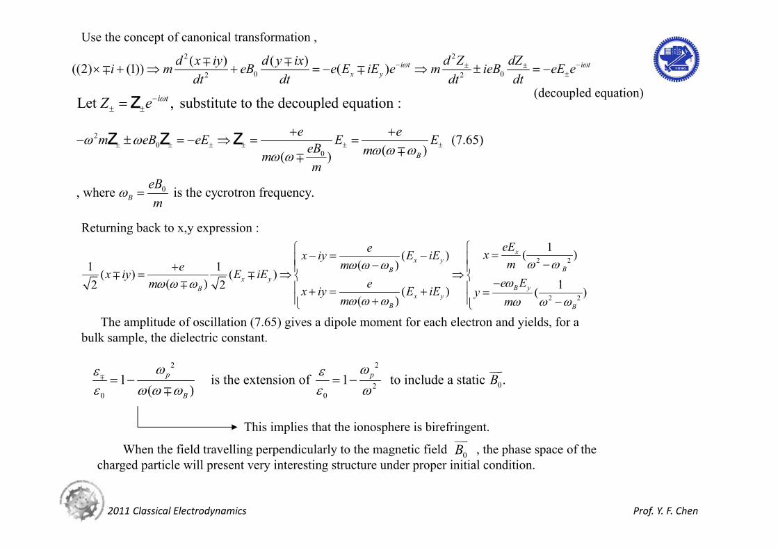
Use the concept of canonical transformation , 22
0 02 2
( ) ( )((2) (1)) ( ) i t i tx y
d Z dZd x iy d y ixi m eB e E iE e m ieB eE edt dt dt dt
Let , substitute to the decoupled equation :i tZ e Z
(decoupled equation)
20
0
0
(7.65) ( )( )
, where is the cycrotron frequency.
B
B
e em eB eE E EeB mmm
eBm
Z Z Z
Returning back to x,y expression :
2 2
2 2
1( )( )( )1 1( ) ( )
( ) 12 2 ( ) ( )( )
xx y
BBx y
B yBx y
B B
eEe xx iy E iEmmex iy E iE
e Eem x iy E iE ym m
The amplitude of oscillation (7.65) gives a dipole moment for each electron and yields, for a bulk sample, the dielectric constant.
2 2
020 0
1 is the extension of 1 to include a static .( )
p p
B
B
This implies that the ionosphere is birefringent.
When the field travelling perpendicularly to the magnetic field , the phase space of the charged particle will present very interesting structure under proper initial condition.
0B
A First Look at Quantum Physics
2011 Classical Electrodynamics Prof. Y. F. Chen
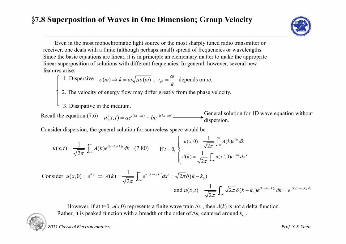
§7.8 Superposition of Waves in One Dimension; Group Velocity
Even in the most monochromatic light source or the most sharply tuned radio transmitter or receiver, one deals with a finite (although perhaps small) spread of frequencies or wavelengths. Since the basic equations are linear, it is in principle an elementary matter to make the approprite linear superposition of solutions with different frequencies. In general, however, several new features arise:
1. Dispersive :
2. The velocity of energy flow may differ greatly from the phase velocity.
3. Dissipative in the medium.
( ) ( ) , depends on .phk vk
Recall the equation (7.6) ( ) ( )( , ) i kx t i kx tu x t ae be General solution for 1D wave equation without dispersion.
Consider dispersion, the general solution for sourceless space would be
( )1( , ) ( ) (7.80)2
ikx i k tu x t A k e dk
'
1( ,0) ( )2If 0,
1( ) ( ',0) '2
ikx
ikx
u x A k e dkt
A k u x e dx
0 0( ) '0
1Consider ( ,0) ( ) ' 2 ( )2
ik x i k k xu x e A k e dx k k
0 0( ( ) )( )0
1and ( , ) 2 ( )2
i k x k tikx i k tu x t k k e dk e
However, if at t=0, u(x,0) represents a finite wave train Δx , then A(k) is not a delta-function. Rather, it is peaked function with a breadth of the order of Δk, centered around k0 .
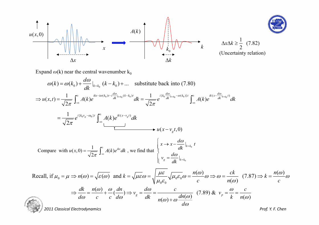
2011 Classical Electrodynamics Prof. Y. F. Chen
x
( ,0)u x
x
( )A k
k0k
k
1 (7.82)2
x k
(Uncertainty relation)
Expand ω(k) near the central wavenumber k0
00 0( ) ( ) | ( ) ... substitute back into (7.80)k kdk k k kdk
0 0 0 00 0 0( ) | ( ) { | ( )} ( | )1 1( , ) ( ) ( )2 2
k k k k k kd d dikx i k t i k k t i k k t ik x tdk dk dku x t A k e dk e A k e dk
0 0{ } ( )1 ( )2
g gi k v t ik x v te A k e dk
( ,0)gu x v t
0
0
|1Compare with ( ,0) ( ) , we find that 2 |
k kikx
g k k
dx x tdku x A k e dk
dvdk
0 0 00 0
( ) ( )Recall, if ( ) ( ) and (7.87)( )
n ck nn k kc n c
( ) ( ) (7.89) & ( ) ( )( )g p
dk n dn d c cv vdnd c c d dk k nnd
2011 Classical Electrodynamics Prof. Y. F. Chen
§7.9 Illustration of the Spreading of a Pulse as it Propagates in a Dispersive Medium
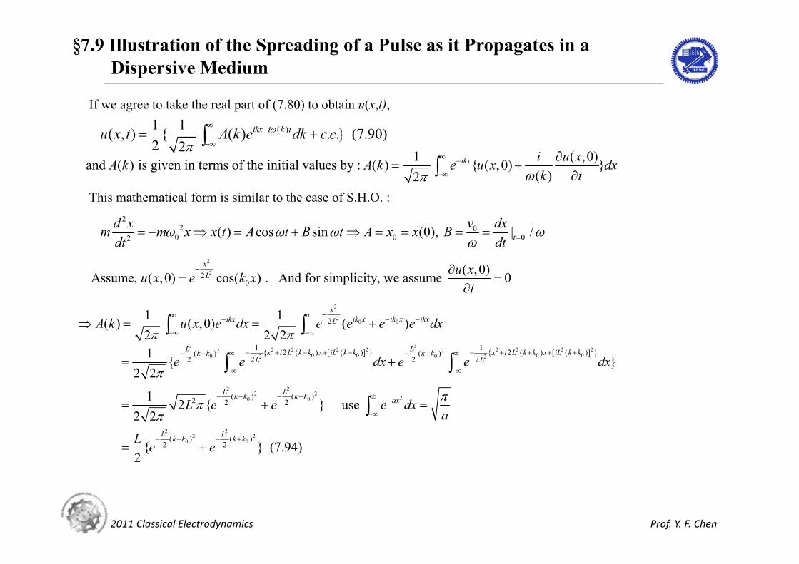
If we agree to take the real part of (7.80) to obtain u(x,t),
( )1 1( , ) { ( ) . .} (7.90)2 2
ikx i k tu x t A k e dk c c
1 ( ,0) and ( ) is given in terms of the initial values by : ( ) { ( ,0) }( )2
ikx i u xA k A k e u x dxk t
This mathematical form is similar to the case of S.H.O. :
22 0
0 0 02 ( ) cos sin (0), | /tvd x dxm m x x t A t B t A x x B
dt dt
2
220
( ,0)Assume, ( ,0) cos( ) . And for simplicity, we assume 0xL u xu x e k x
t
2
2 0 021 1( ) ( ,0) ( )2 2 2
xik x ik xikx ikxLA k u x e dx e e e e dx
2 22 2 2 2 2 2 2 22 2
0 0 0 00 02 21 1{ 2 ( ) [ ( )] } { 2 ( ) [ ( )] }( ) ( )
2 2 2 21 { }2 2
L Lx i L k k x iL k k x i L k k x iL k kk k k kL Le e dx e e dx
2 22 2
20 0( ) ( )2 2 21 2 { } use 2 2
L Lk k k k axL e e e dxa
2 22 2
0 0( ) ( )2 2{ } (7.94)
2
L Lk k k kL e e
2011 Classical Electrodynamics Prof. Y. F. Chen
2 2
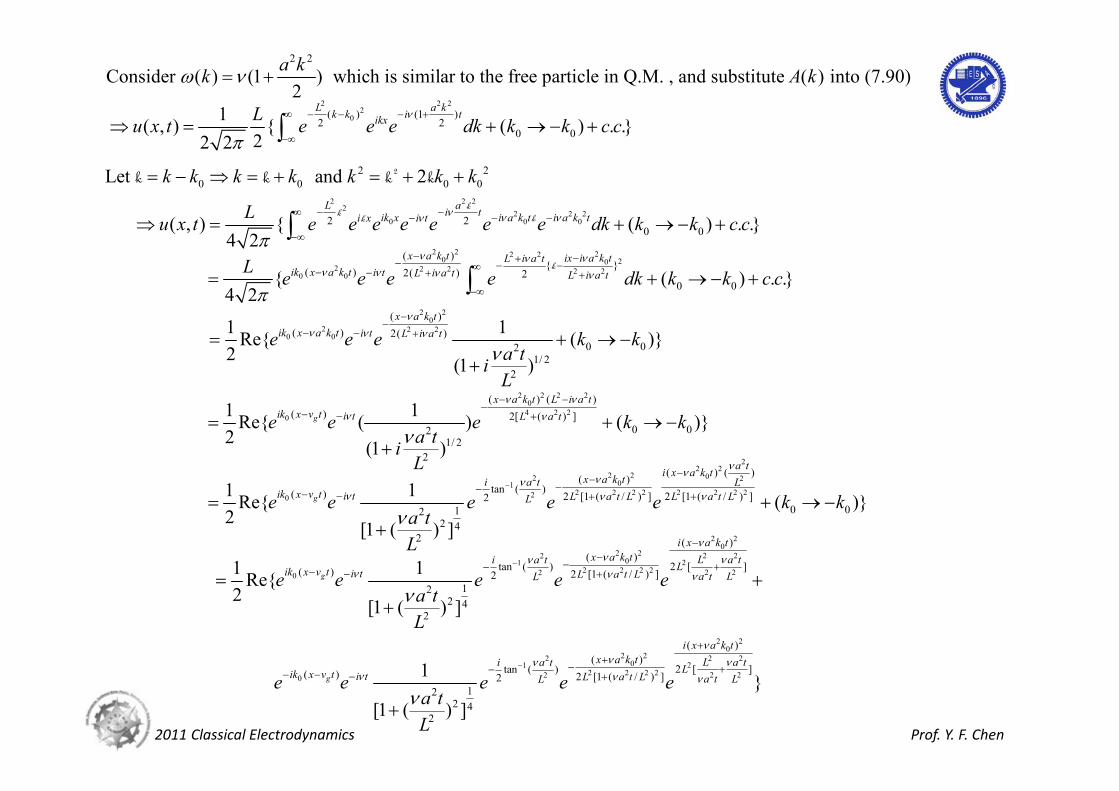
Consider ( ) (1 ) which is similar to the free particle in Q.M. , and substitute ( ) into (7.90)2
a kk A k 2 2 2
20( ) (1 )
2 20 0
1( , ) { ( ) . .}22 2
L a kk k i tikxLu x t e e e dk k k c c
2 20 0 0 0Let and 2k k k k k k k 2k k k k
2 2 22
2 2 20 0 02 2
0 0( , ) { ( ) . .}4 2
L ai tik x i a k t i a k ti x i tLu x t e e e e e e e dk k k c c
kk kk
2 2 22 20 202 2 2 2 20 0
( ){ }( ) 2( ) 2
0 0{ ( ) . .}4 2
x a k t ix i a k tL i a tik x a k t i t L i a t L i a tL e e e e dk k k c c
k
2 20
2 2 20 0
( )( ) 2( )
0 021/ 2
2
1 1Re{ ( )}2 (1 )
x a k tik x a k t i t L i a te e e k k
a tiL
2 2 2 20
4 2 20
( ) ( )( ) 2[ ( ) ]
0 021/ 2
2
1 1Re{ ( ) ( )}2 (1 )
g
x a k t L i a tik x v t i t L a te e e k k
a tiL
22 2
2 2 02 2012 2 2 2 2 2 2 220
( ) ( )( )tan ( )( ) 2 [1 ( / ) ] 2 [1 ( / ) ]2
0 0122 4
2
1 1Re{ ( )}2 [1 ( ) ]
g
a ti x a k tx a k ti a t Lik x v t i t L a t L L a t LLe e e e e k k
a tL
2 20
2 2 2 22 0 212 2 2 2 2 220
2 22 01220
( )( )
2 [ ]tan ( )( ) 2 [1 ( / ) ]212
2 42
( )tan ( )( ) 2 [1 (2
122 4
2
1 1Re{2 [1 ( ) ]
1 [1 ( ) ]
g
g
i x a k tx a k t L a ti a t Lik x v t i t L a t L a t LL
x a k ti a tik x v t i t LL
e e e e ea tL
e e e ea tL
2 20
2 22
2 2 2 2 2
( )
2 [ ]/ ) ] }
i x a k tL a tL
a t L a t Le
2011 Classical Electrodynamics Prof. Y. F. Chen
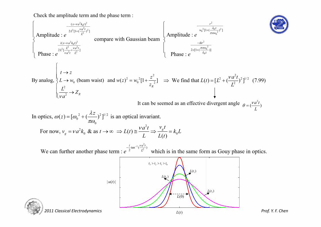
Check the amplitude term and the phase term :22 2
02 2 202 2 0 22 0
22 20
22 202
2 20
( )
[1 ( ) ]2 [1 ( ) ]
( )
2 [1 ( )]2 [ ]
Amplitude : Amplitude : compare with Gaussian beam
Phase : Phase :
rx a k tza t wL nwL
ikri x a k tnwL a t zL
za t L
ee
e e
22 2
0 0 22
2
By analog, (beam waist) and ( ) [1 ]
R
R
t zzL w w z wz
L Za
22 2 1/ 2
2We find that ( ) [ ( ) ] (7.99)a tL t LL
It can be seemed as an effective divergent angle 2
( )a tL
2 2 1/ 20
0
In optics, ( ) [ ( ) ] is an optical invariant. zz
2
20 0For now, & as ( )
( )g
g
v ta tv a k t L t k LL L t
21
2tan ( )2We can further another phase term : which is in the same form as Gouy phase in optics.i a t
Le
(0)L
1( )L t
2( )L t
3( )L t
3 2 1 0t t t t
( )L t
| ( ) |u t
2011 Classical Electrodynamics Prof. Y. F. Chen
§7.10 Causality in the Connection Between ;Kramers-Kronig Relations
D and E
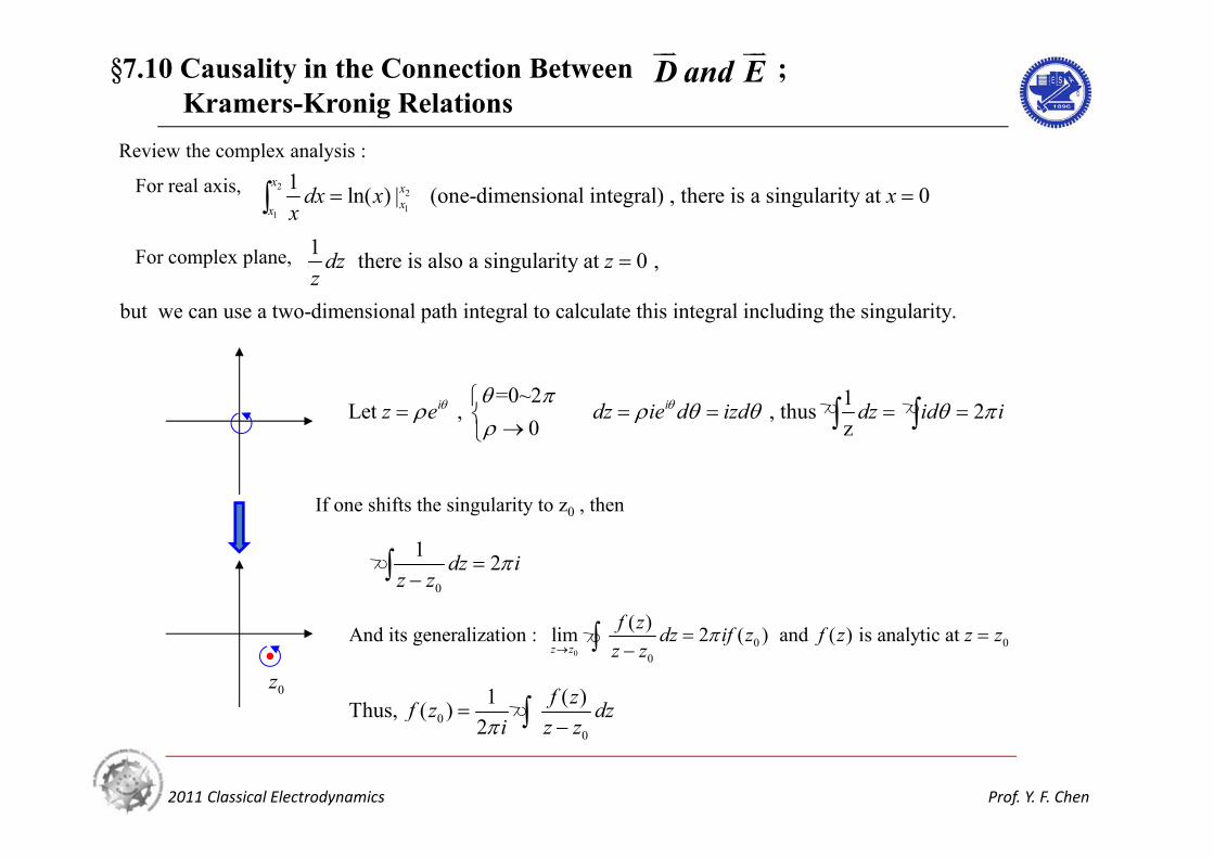
Review the complex analysis :
For real axis, 22
11
1 ln( ) | (one-dimensional integral) , there is a singularity at 0 x x
xxdx x x
x
For complex plane, 1 there is also a singularity at 0 , dz zz
but we can use a two-dimensional path integral to calculate this integral including the singularity.
=0~2 1Let , , thus 20 z
i iz e dz ie d izd dz id i
0z
If one shifts the singularity to z0 , then
0
1 2dz iz z
00 0
0
( )And its generalization : lim 2 ( ) and ( ) is analytic at z z
f z dz if z f z z zz z
00
1 ( )Thus, ( ) 2
f zf z dzi z z
In reality, the finite response time and the finite transfer speed for information produce a temporally nonlocal connection between the input disturbance and the output response.
2011 Classical Electrodynamics Prof. Y. F. Chen
For system with infinite information transfer speed, the impulse response will be a delta-function.
A. Non-locality in time In previous chapter, we consider ( , ) ( , ) , where is constant.D x t E x t
We know in more realistic case, the dielectric would be a function of .
Under linear response approximation, which means both ( , ) and ( , ) correspond to the same .x x D E
( , ) ( ) ( , ) (7.103)x x D E
'1 1And ( , ) ( , ) & ( , ) ( , ') '2 2
i t i tD x t x e d x D x t e dt
D D
'1 1( , ) ( ) ( , ) ; ( , ) ( , ') '2 2
i t i tD x t x e d x E x t e dt
E E
( ') ( ')
-
1 1( , ) ' ( ) ( , ') ( ( ) ) ( , ') '2 2
i t t i t tD x t d dt E x t e e d E x t dt
0 0 0 0 0 0 2 20
( )
( )We know that ( )= ( ( ) ) ( 1)( )
e
j
j j j
fi
( ') ( ')0 0 0 0
1 1( , ) ( { ( )} ) ( , ') ' ( , ) { '( ( ) ) ( , ')}2 2
i t t i t te eD x t e d E x t dt E x t dt e d E x t
Let ' ' & 't t t t dt d
Define the response function of the system ( ) : G -i
-0
1 ( )( ) ( -1)e 2
G d
2011 Classical Electrodynamics Prof. Y. F. Chen
0
simultaneous response time-delay response
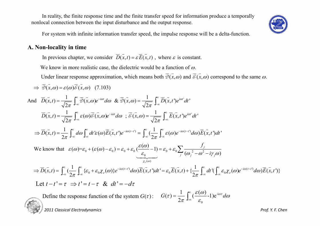
And ( , ) { ( , ) ( ) ( , ) } (7.105)D x t E x t G E x t d
0
( )G
The effective contribution for is from , which will be proven later.( )G 0 ~
B. Simple Model for G(τ), Limitations 2
e 2 20 0
( )Recall, ( ) ( 1)( )
j
j j j
fNem i
2
e 2 20
Assume single resonant mode ( ) (7.107)( )
p
i
2
2 20
1Thus, ( ) (7.108)2 ( )
ip e
G di
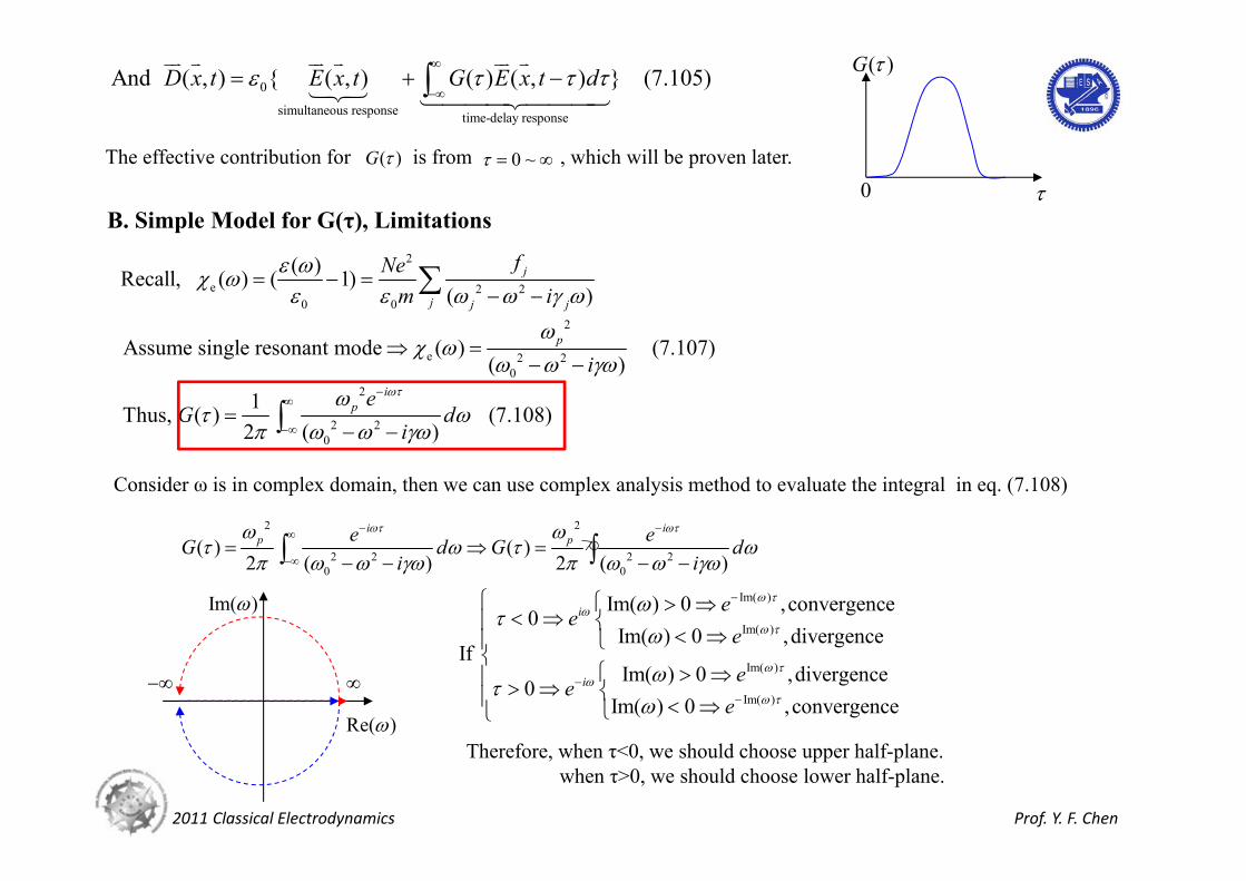
Consider ω is in complex domain, then we can use complex analysis method to evaluate the integral in eq. (7.108)
2 2
2 2 2 20 0
( ) ( )2 ( ) 2 ( )
i ip pe eG d G d
i i
Re( )
Im( ) Im( )
Im( )
Im( )
Im( )
Im( ) 0 ,convergence0
Im( ) 0 ,divergenceIf
Im( ) 0 ,divergence0
Im( ) 0 ,convergence
i
i
ee
e
ee
e
Therefore, when τ<0, we should choose upper half-plane.when τ>0, we should choose lower half-plane.
2011 Classical Electrodynamics Prof. Y. F. Chen
2 2 22 2 2 2 2 2 2
0 0 0 0Consider 0 ( ) 0 ( )4 4 2 4
ii i
22
1 0 0
22
2 0 0
2 4 2The two roots :
2 4 2
i i
i i
Re( )
Im( )
00
2
2 2
1 2 1 2 1 2
1( ) [ ]2 ( )( ) 2 ( ) ( ) ( )
i i ip pe e eG d d
1 21 2
2 2
1 2 2 1 2 1
1( ) ( 2 ) ( ) ( 2 )2 ( ) ( ) 2 ( )
i ip p i ie e i e e i
0 0
2 22 2 2
02 1 0
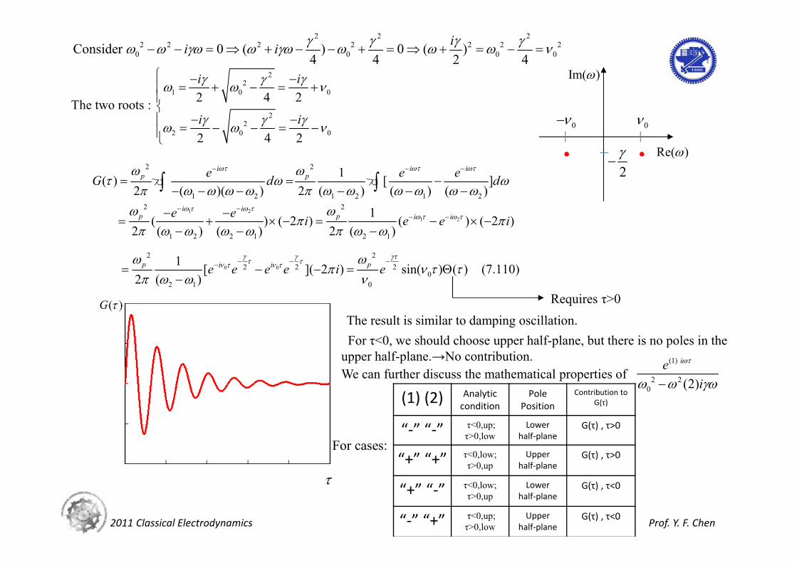
1 [ ]( 2 ) sin( ) ( ) (7.110)2 ( )
p pi ie e e e i e
Requires τ>0( )G
The result is similar to damping oscillation.For τ<0, we should choose upper half-plane, but there is no poles in the
upper half-plane.→No contribution.We can further discuss the mathematical properties of
(1)
2 20 (2)
iei
For cases:
(1) (2) Analytic condition
PolePosition
Contribution to G(τ)
“‐” “‐” τ<0,up;τ>0,low
Lower half‐plane
G(τ) , τ>0
“+” “+” τ<0,low;τ>0,up
Upper half‐plane
G(τ) , τ>0
“+” “‐” τ<0,low;τ>0,up
Lower half‐plane
G(τ) , τ<0
“‐” “+” τ<0,up;τ>0,low
Upper half‐plane
G(τ) , τ<0
2011 Classical Electrodynamics Prof. Y. F. Chen
C. Causality and Analyticity Domain of ε(ω)2
2 022 2
0 0
sin( )( ) ( )2 ( )
ip
peG d e
i
This kernel vanishes for τ<0.The result means that at time t, only values of the electric field prior to that time enter in determining the
displacement in accord with our fundamental ideas of causality in physical phenomena.
0 0(Recall) ( , ) { ( , ) ( ) ( , ) } (7.111)D x t E x t G E x t d
Its validity transcends any specific model of ε(ω).
00 0
1 ( ) ( )From (7.106) ( ) ( 1) 1 ( ) (7.112)2
i iG e d G e d
The behavior of for large ω can be related to the behavior of G(τ) at small time difference.0
( ) 1
00 00
( ) 11 ( ) 1 ( )( ) | ( ) '( )i i iiG e d G e G e di
2 31 (0) ( ) '(0) ( ) ''(0) ......i i iG G G
G(0-)=0, G(0+)≠0 is unphysical. → The first term in the series is absent and falls off at high frequencies as ω-2. 0
( ) 1
The asymptotic series shows, in fact, that the real and imaginary parts of behave for large real ω as,0
( ) 1
2 30 0
( ) 1 ( ) 1Re( 1) ( ) ; Im( ) ( )O O
D. Kramers-Kronig Relations
2011 Classical Electrodynamics Prof. Y. F. Chen
The analyticity of ε(ω)/ε0 in the upper half- ω-plane permits the use of Cauchy’s theorem to relate the real and imaginary parts of ε(ω)/ε0 on the real axis.
For any point z inside the close contour C in the upper half- ω-plane :
0C
0
( ( ') / ) 1( ) 11 ' , where and let 02 '
z d z ii z
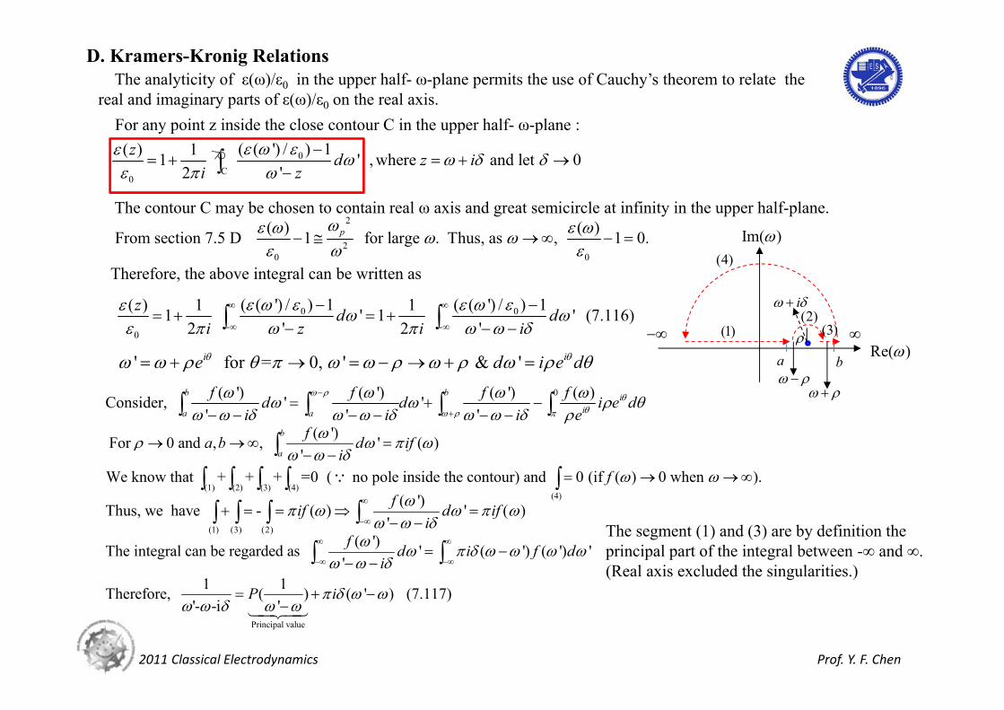
The contour C may be chosen to contain real ω axis and great semicircle at infinity in the upper half-plane.2
20 0
( ) ( )From section 7.5 D 1 for large . Thus, as , 1 0.p
Therefore, the above integral can be written as
0 0- -
0
( ( ') / ) 1 ( ( ') / ) 1( ) 1 11 ' 1 ' (7.116)2 ' 2 '
z d di z i i
Re( )
Im( )
a b
i
(4)
(1)(2)
(3)
' for = 0, ' & 'i ie d i e d 0( ') ( ') ( ') ( )Consider, ' '
' ' 'b b i
ia a
f f f fd d i e di i i e
( ')For 0 and , , ' ( )
'b
a
fa b d ifi
(1) (2) (3) (4)(4)
We know that + + + =0 ( no pole inside the contour) and 0 (if ( ) 0 when ). f
(1) (3) (2)
( ')Thus, we have - ( ) ' )'fif d if
i
( ')The integral can be regarded as ' ( ') ( ') '
'f d i f d
i
The segment (1) and (3) are by definition the principal part of the integral between -∞ and ∞.(Real axis excluded the singularities.)
Principal value
1 1Therefore, ( ) ( ' ) (7.117)'- -i '
P i
2011 Classical Electrodynamics Prof. Y. F. Chen
-0 0
( ) 1 ( ') 1Substitute (7.1170 back into (7.116) 1 ( 1)[ ( ( ' )] '.2 '
z P i di
0
-0 0 0
( ( ') / ) 11 ( ') 1 ( ) ( ) 1 And ( 1) ( ' ) ' ( 1) 1 '2 2 '
i d P di i
0 0
0 0 0
Im( ( ') / ) Re[( ( ') / ) 1]( ) ( ) 1 ( ) 1For is complex, Re( ) 1 ' & Im( ) ' ' '
P d P d
0 02 2 2 2
' Im( ( ') / ) Im( ( ') / )' '' '
Multiply ( '+ ) on the integrandP d P d
02 2
'Re[( ( ') / ) 1] ''
P d
02 2
Re[( ( ') / ) 1]+ ' '
P d
for real ( ) ( ), even functionRecall: ( ) *( *) ( is complex but is real.)
for imaginary ( ) ( ), odd function
0 02 2 2 20 0
0 0
' Im( ( ') / ) Re[( ( ') / ) 1]( ) 2 ( ) 2We have Re( ) 1 ' & Im( ) ' (7.120) ' '
P d P d
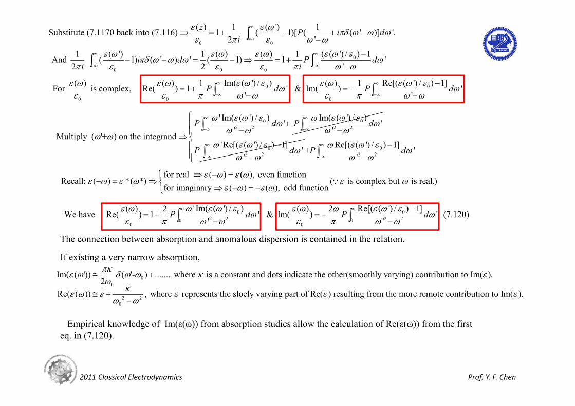
The connection between absorption and anomalous dispersion is contained in the relation.
If existing a very narrow absorption,
00
Im( ( ')) ( '- ) ......, where is a constant and dots indicate the other(smoothly varying) contribution to Im( ).2
2 20
Re( ( )) , where represents the sloely varying part of Re( ) resulting from the more remote contribution to Im( ).
Empirical knowledge of Im(ε(ω)) from absorption studies allow the calculation of Re(ε(ω)) from the first eq. in (7.120).

2011 Classical Electrodynamics Prof. Y. F. Chen
Consider the incidence of plane wave: ~ ; 2
ikze k i
0I
ikze
d
I
00
1Use ln( )z II I ed I
1 2 1 2For & 2 2
kn in i k i
k n
1 2 22 2 2
1 2 1
22We have & 2
n nn
n n
There are two ways to obtain the information for ε and n :
(1) Measure α to obtain n2, then substitute it into the K-K relation to iterate (first assume a value for n1 )until reach a self-consistent result.
(2) ε=ε1+iε2 Use simple-harmonic oscillator model to find an analytic fitting function with parameters fj, ωj, ϒj , then calculate n1 ,n2 , ε1, ε2.
22 2
20 0
( ) ( )Sum rule : from (7.59) lim 1 lim (1 )pp
2 2 2002 20 0
0
' Im[ ( ') / ]2 ( ) 2lim ' lim [1 Re( )] ' Im[ ( ') / ] ' (7.122)' pP d d
2
2
0
Recall, and ; j pj
nef Z n NZm
2011 Classical Electrodynamics Prof. Y. F. Chen
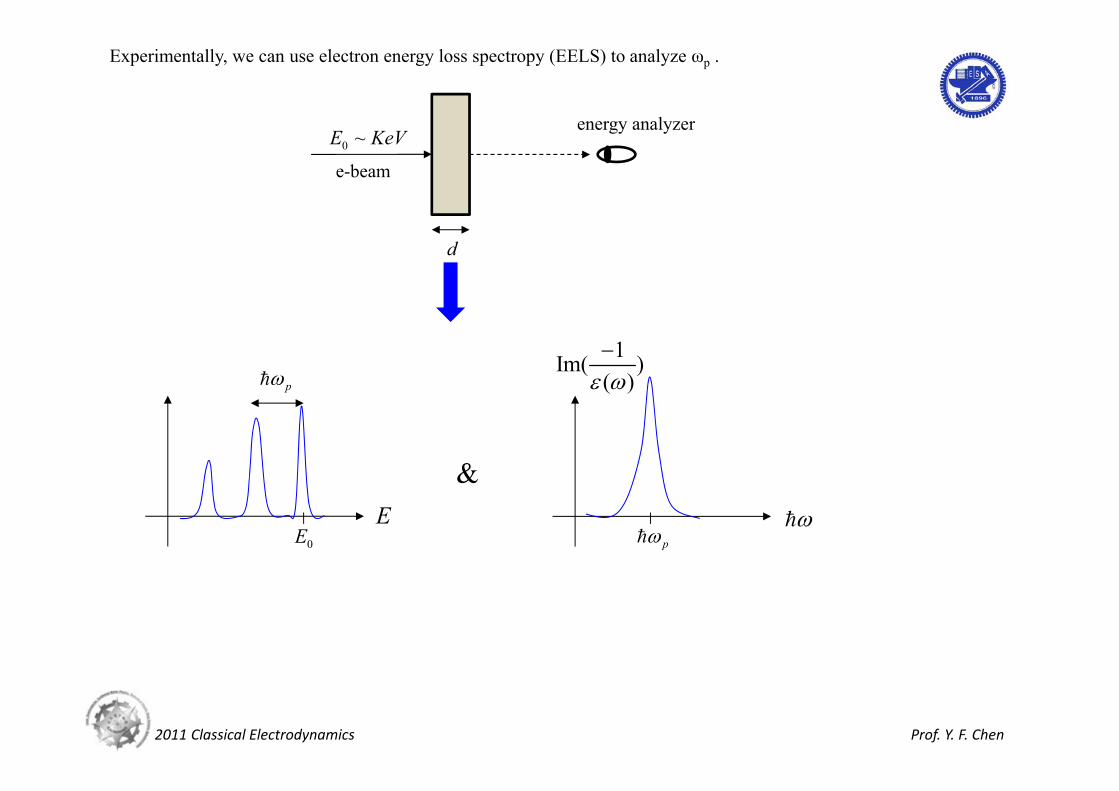
Experimentally, we can use electron energy loss spectropy (EELS) to analyze ωp .
0 ~E KeV
e-beam
d
energy analyzer
E0E
p
p
1Im( )( )
&