plane frame and grid equations - the university of … 5a – plane frame and grid equations...
TRANSCRIPT

Chapter 5a – Plane Frame and Grid Equations
Learning Objectives• To derive the two-dimensional arbitrarily oriented
beam element stiffness matrix
• To demonstrate solutions of rigid plane frames by the direct stiffness method
• To describe how to handle inclined or skewed supports
Plane Frame and Grid EquationsMany structures, such as buildings and bridges, are
composed of frames and/or grids.
This chapter develops the equations and methods for solution of plane frames and grids.
First, we will develop the stiffness matrix for a beam element arbitrarily oriented in a plane.
CIVL 7/8117 Chapter 5 - Plane Frame and Grid Equations - Part 1 1/52

Plane Frame and Grid EquationsMany structures, such as buildings and bridges, are
composed of frames and/or grids.
We will then include the axial nodal displacement degree of freedom in the local beam element stiffness matrix.
Plane Frame and Grid EquationsMany structures, such as buildings and bridges, are
composed of frames and/or grids.
Then we will combine these results to develop the stiffness matrix, including axial deformation effects, for an arbitrarily oriented beam element.
We will also consider frames with inclined or skewed supports.
CIVL 7/8117 Chapter 5 - Plane Frame and Grid Equations - Part 1 2/52

Plane Frame and Grid EquationsTwo-Dimensional Arbitrarily Oriented Beam Element
We can derive the stiffness matrix for an arbitrarily oriented beam element, in a manner similar to that used for the bar element.
The local axes and are located along the beam element and transverse to the beam element, respectively, and the global axes x’ and y’ are located to be convenient for the total structure.
Plane Frame and Grid EquationsTwo-Dimensional Arbitrarily Oriented Beam Element
The transformation from local displacements to global displacements is given in matrix form as:
Using the second equation for the beam element, we can relate local nodal degrees of freedom to global degree of freedom:
cos
sin
u C S u C
v S C v S
1
1 1
1 1
2 2
2 2
2
0 0 0 0
0 0 1 0 0 0
0 0 0 0
0 0 0 0 0 1
u
v vS C
v uS C
v
1 1 1v Su Cv
d Td
CIVL 7/8117 Chapter 5 - Plane Frame and Grid Equations - Part 1 3/52

Plane Frame and Grid EquationsTwo-Dimensional Arbitrarily Oriented Beam Element
For a beam, we will define the following as the transformation matrix:
Notice that the rotations are not affected by the orientation of the beam.
0 0 0 0
0 0 1 0 0 0
0 0 0 0
0 0 0 0 0 1
S C
S C
T
Plane Frame and Grid EquationsTwo-Dimensional Arbitrarily Oriented Beam Element
Substituting the above transformation into the general form of the stiffness matrix TTk’T gives:
1 1 1 2 2 2
2 2
2 2
2 2
3 2 2
2 2
2 2
12 12 6 12 12 6
12 12 6 12 12 6
6 6 4 6 6 2
12 12 6 12 12 6
12 12 6 12 12 6
6 6 2 6 6 4
u v u v
S SC LS S SC LS
SC C LC SC C LC
LS LC L LS LC LEI
L S SC LS S SC LS
SC C LC SC C LC
LS LC L LS LC L
k
CIVL 7/8117 Chapter 5 - Plane Frame and Grid Equations - Part 1 4/52
Plane Frame and Grid EquationsTwo-Dimensional Arbitrarily Oriented Beam Element
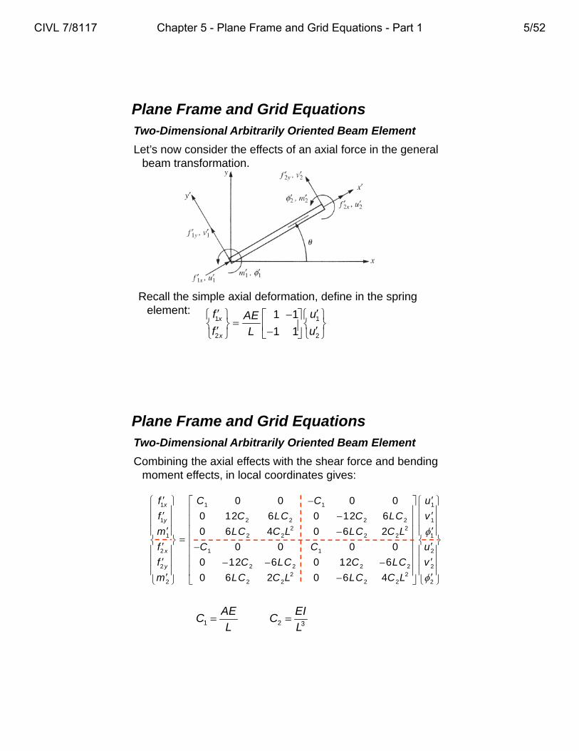
Let’s now consider the effects of an axial force in the general beam transformation.
Recall the simple axial deformation, define in the spring element:
1 1
2 2
1 1
1 1x
x
f uAEf uL
Plane Frame and Grid EquationsTwo-Dimensional Arbitrarily Oriented Beam Element
Combining the axial effects with the shear force and bending moment effects, in local coordinates gives:
1 1 1 1
1 2 2 2 2 12 2
1 2 2 2 2 1
2 1 1 2
2 2 2 2 2 22 2
2 2 2 2 2 2
0 0 0 0
0 12 6 0 12 6
0 6 4 0 6 2
0 0 0 0
0 12 6 0 12 6
0 6 2 0 6 4
x
y
x
y
f C C u
f C LC C LC v
m LC C L LC C L
f C C u
f C LC C LC v
m LC C L LC C L
1 2 3
AE EIC C
L L
CIVL 7/8117 Chapter 5 - Plane Frame and Grid Equations - Part 1 5/52

Plane Frame and Grid EquationsTwo-Dimensional Arbitrarily Oriented Beam Element
Therefore:
1 1
2 2 2 22 2
2 2 2 2
1 1
2 2 2 22 2
2 2 2 2
0 0 0 0
0 12 6 0 12 6
0 6 4 0 6 2
0 0 0 0
0 12 6 0 12 6
0 6 2 0 6 4
C C
C LC C LC
LC C L LC C L
C C
C LC C LC
LC C L LC C L
k
The above stiffness matrix include the effects of axial force in the x’ direction, shear force in the y’ direction, and bending moment about the z’ axis.
Plane Frame and Grid EquationsTwo-Dimensional Arbitrarily Oriented Beam Element
The local degrees of freedom may be related to the global degrees of freedom by:
where T has been expanded to include axial effects
1 1
1 1
1 1
2 2
2 2
2 2
0 0 0 0
0 0 0 0
0 0 1 0 0 0
0 0 0 0
0 0 0 0
0 0 0 0 0 1
u uC S
v vS C
u uC S
v vS C
d Td
CIVL 7/8117 Chapter 5 - Plane Frame and Grid Equations - Part 1 6/52
Plane Frame and Grid EquationsTwo-Dimensional Arbitrarily Oriented Beam Element
Substituting the above transformation T into the general form of the stiffness matrix gives:
2 2 2 2
2 2 2 2
2 2 2 22 2 2
2 22 2
2 2
2
12 12 6 12 12 6
12 6 12 12 6
6 64 2
12 12 6
12 6
4
I I I I I IAC S A CS S AC S A CS S
L LL L L L
I I I I IAS C C A CS AS C C
L LL L L
I IE I S C Ik L LLI I I
AC S A CS SLL L
I Isymmetric AS C C
LLI
Plane Frame and Grid EquationsTwo-Dimensional Arbitrarily Oriented Beam Element
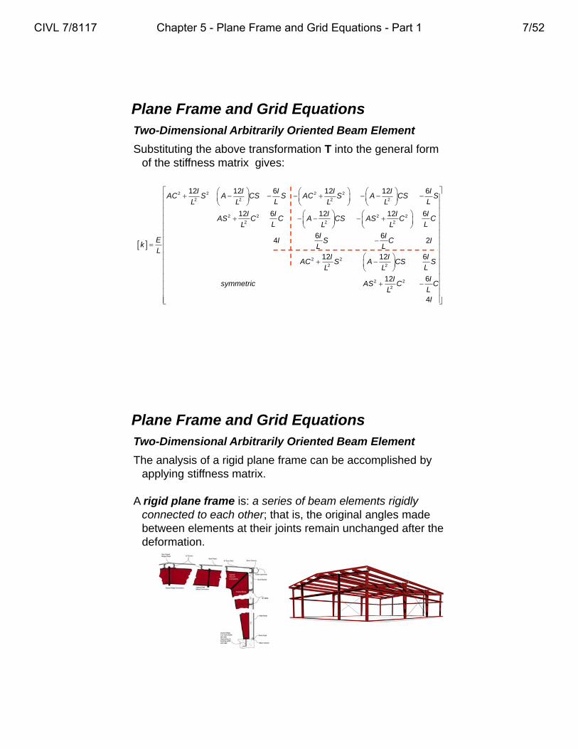
The analysis of a rigid plane frame can be accomplished by applying stiffness matrix.
A rigid plane frame is: a series of beam elements rigidly connected to each other; that is, the original angles made between elements at their joints remain unchanged after the deformation.
CIVL 7/8117 Chapter 5 - Plane Frame and Grid Equations - Part 1 7/52

Plane Frame and Grid EquationsTwo-Dimensional Arbitrarily Oriented Beam Element
Furthermore, moments are transmitted from one element to another at the joints.
Hence, moment continuity exists at the rigid joints.
Plane Frame and Grid EquationsTwo-Dimensional Arbitrarily Oriented Beam Element
In addition, the element centroids, as well as the applied loads, lie in a common plane.
We observe that the element stiffnesses of a frame are functions of E, A, L, I, and the angle of orientation of the element with respect to the global-coordinate axes.
CIVL 7/8117 Chapter 5 - Plane Frame and Grid Equations - Part 1 8/52

Plane Frame and Grid EquationsRigid Plane Frame Example 1
Consider the frame shown in the figure below.
The frame is fixed at nodes 1 and 4 and subjected to a positive horizontal force of 10,000 lb applied at node 2 and to a positive moment of 5,000 lb-in applied at node 3.
Plane Frame and Grid EquationsRigid Plane Frame Example 1
Consider the frame shown in the figure below.
Let E = 30 x 106 psi and A = 10 in2 for all elements, and let I = 200 in4 for elements 1 and 3, and I = 100 in4 for element 2.
CIVL 7/8117 Chapter 5 - Plane Frame and Grid Equations - Part 1 9/52

Plane Frame and Grid EquationsRigid Plane Frame Example 1
Element 1: The angle between x and x’ is 90°
0 1C S
2 3
22
12 12(200) 6 6(200)0.167 10.0
120120
I Iin in
L L
6
3
30 10250,000
120
E lbinL
Plane Frame and Grid EquationsRigid Plane Frame Example 1
Element 1: The angle between x and x’ is 90°
1 1 1 2 2 2
(1)
0.167 0 10 0.167 0 10
0 10 0 0 10 0
10 0 800 10 0 400250,000
0.167 0 10 0.167 0 10
0 10 0 0 10 0
10 0 400 10 0 800
u v u v
lbin
k
CIVL 7/8117 Chapter 5 - Plane Frame and Grid Equations - Part 1 10/52

Plane Frame and Grid EquationsRigid Plane Frame Example 1
Element 2: The angle between x and x’ is 0°
1 0C S
2 3
22
12 12(100) 6 6(100)0.0835 5.0
120120
I Iin in
L L
6
3
30 10250,000
120
E lbinL
2 2 2 3 3 3
(2)
10 0 0 10 0 0
0 0.0835 5 0 0.0835 5
0 5 400 0 5 200250,000
10 0 0 10 0 0
0 0.0835 5 0 0.0835 5
0 5 200 0 5 400
u v u v
lbin
k
Plane Frame and Grid EquationsRigid Plane Frame Example 1
Element 2: The angle between x and x’ is 0°
CIVL 7/8117 Chapter 5 - Plane Frame and Grid Equations - Part 1 11/52

Plane Frame and Grid EquationsRigid Plane Frame Example 1
Element 3: The angle between x and x’ is 270°
0 1C S
2 3
22
12 12(200) 6 6(200)0.167 10.0
120120
I Iin in
L L
6
3
30 10250,000
120
E lbinL
3 3 3 4 4 4
(3)
0.167 0 10 0.167 0 10
0 10 0 0 10 0
10 0 800 10 0 400250,000
0.167 0 10 0.167 0 10
0 10 0 0 10 0
10 0 400 10 0 800
u v u v
lbin
k
Plane Frame and Grid EquationsRigid Plane Frame Example 1
Element 3: The angle between x and x’ is 270°
CIVL 7/8117 Chapter 5 - Plane Frame and Grid Equations - Part 1 12/52

Plane Frame and Grid EquationsRigid Plane Frame Example 1
The boundary conditions for this problem are:
1 1 1 4 4 4 0u v u v
After applying the boundary conditions the global beam equations reduce to:
2
2
25
3
3
3
10,000 10.167 0 10 10 0 0
0 0 10.0835 5 0 0.0835 5
0 10 5 1200 0 5 2002.5 10
0 10 0 0 10.167 0 10
0 0 0.0835 5 0 10.0835 5
5,000 0 5 200 10 5 1200
u
v
u
v
2 2 2 3 3 3u v u v
Plane Frame and Grid EquationsRigid Plane Frame Example 1
Solving the above equations gives: 2
2
2
3
3
3
0.211
0.00148
0.00153
0.209
0.00148
0.00149
u in
v in
rad
u in
v in
rad
x
y
CIVL 7/8117 Chapter 5 - Plane Frame and Grid Equations - Part 1 13/52

Plane Frame and Grid EquationsRigid Plane Frame Example 1
Solving the above equations gives:
x
y
Plane Frame and Grid EquationsRigid Plane Frame Example 1
Element 1: The element force-displacement equations can be obtained using f’ = k’Td. Therefore, Td is:
1
1
1
2
2
2
00 1 0 0 0 0
01 0 0 0 0 0
00 0 1 0 0 0
0.2110 0 0 0 1 0
0.001480 0 0 1 0 0
0.001530 0 0 0 0 1
u
v
u in
v in
rad
Td
0 1C S
0
0
0
0.00148
0.211
0.00153
in
in
rad
0 0 0 0
0 0 0 0
0 0 1 0 0 0
0 0 0 0
0 0 0 0
0 0 0 0 0 1
C S
S C
TC S
S C
CIVL 7/8117 Chapter 5 - Plane Frame and Grid Equations - Part 1 14/52

Plane Frame and Grid EquationsRigid Plane Frame Example 1
Element 1: Recall the elemental stiffness matrix is:
1 1
2 2 2 22 2
2 2 2 2
1 1
2 2 2 22 2
2 2 2 2
0 0 0 0
0 12 6 0 12 6
0 6 4 0 6 2
0 0 0 0
0 12 6 0 12 6
0 6 2 0 6 4
C C
C LC C LC
LC C L LC C L
C C
C LC C LC
LC C L LC C L
k
(1) 5
10 0 0 10 0 0 0
0 0.167 10 0 0.167 10 0
0 10 800 0 10 400 02.5 10
10 0 0 10 0 10 0.00148
0 0.167 10 0 0.167 10 0.211
0 10 400 0 10 800 0.00153
in
in
rad
f k Td
The local force-displacement equations are:
4 6
2 33
200 30 103,472.22
120lb
in
in psiEIC
L in
2 6
61
10 30 102.5 10
120lb
in
in psiAEC
L in
Plane Frame and Grid EquationsRigid Plane Frame Example 1
Element 1: Simplifying the above equations gives:
1
1
1
2
2
2
3,700
4,990
376
3,700
4,990
223
x
y
x
y
f lb
f lb
m k in
f lb
f lb
m k in
CIVL 7/8117 Chapter 5 - Plane Frame and Grid Equations - Part 1 15/52

2
2
2
3
3
3
0.2111 0 0 0 0 0
0.001480 1 0 0 0 0
0.001530 0 1 0 0 0
0.2090 0 0 1 0 0
0.001480 0 0 0 1 0
0.001490 0 0 0 0 1
u in
v in
rad
u in
v in
rad
Td
Plane Frame and Grid EquationsRigid Plane Frame Example 1
Element 2: The element force-displacement equations can be obtained using f’ = k’Td. Therefore, Td is:
1 0C S
0 0 0 0
0 0 0 0
0 0 1 0 0 0
0 0 0 0
0 0 0 0
0 0 0 0 0 1
C S
S C
TC S
S C
0.211
0.00148
0.00153
0.209
0.00148
0.00149
in
in
rad
in
in
rad
(2) 5
10 0 0 10 0 0 0.211
0 0.0833 5 0 0.0833 5 0.00148
0 5 400 0 5 200 0.001532.5 10
10 0 0 10 0 0 0.209
0 0.0833 5 0 0.0833 5 0.00148
0 5 200 0 5 400 0.00149
in
in
rad
in
in
rad
f k Td
Plane Frame and Grid EquationsRigid Plane Frame Example 1
Element 2: The local force-displacement equations are:
The local force-displacement equations are:
1 1
2 2 2 22 2
2 2 2 2
1 1
2 2 2 22 2
2 2 2 2
0 0 0 0
0 12 6 0 12 6
0 6 4 0 6 2
0 0 0 0
0 12 6 0 12 6
0 6 2 0 6 4
C C
C LC C LC
LC C L LC C L
C C
C LC C LC
LC C L LC C L
k
2 6
61
10 30 102.5 10
120lb
in
in psiAEC
L in
4 6
2 33
100 30 101,736.11
120lb
in
in psiEIC
L in
CIVL 7/8117 Chapter 5 - Plane Frame and Grid Equations - Part 1 16/52

Plane Frame and Grid EquationsRigid Plane Frame Example 1
Element 2: Simplifying the above equations gives:
2
2
2
3
3
3
5,010
3,700
223
5,010
3,700
221
x
y
x
y
f lb
f lb
m k in
f lb
f lb
m k in
3
3
3
4
4
4
0.2090 1 0 0 0 0
0.001481 0 0 0 0 0
0.001490 0 1 0 0 0
00 0 0 0 1 0
00 0 0 1 0 0
00 0 0 0 0 1
u in
v in
rad
u
v
Td
Plane Frame and Grid EquationsRigid Plane Frame Example 1
Element 3: The element force-displacement equations can be obtained using f’ = k’Td. Therefore, Td is:
0 0 0 0
0 0 0 0
0 0 1 0 0 0
0 0 0 0
0 0 0 0
0 0 0 0 0 1
C S
S C
TC S
S C
0 1C S
0.00148
0.209
0.00149
0
0
0
in
in
rad
CIVL 7/8117 Chapter 5 - Plane Frame and Grid Equations - Part 1 17/52

(3) 5
10 0 0 10 0 0 0.00148
0 0.167 10 0 0.167 10 0.209
0 10 800 0 10 400 0.001492.5 10
10 0 0 10 0 10 0
0 0.167 10 0 0.167 10 0
0 10 400 0 10 800 0
in
in
rad
f k Td
Plane Frame and Grid EquationsRigid Plane Frame Example 1
Element 3: The local force-displacement equations are:
The local force-displacement equations are:
1 1
2 2 2 22 2
2 2 2 2
1 1
2 2 2 22 2
2 2 2 2
0 0 0 0
0 12 6 0 12 6
0 6 4 0 6 2
0 0 0 0
0 12 6 0 12 6
0 6 2 0 6 4
C C
C LC C LC
LC C L LC C L
C C
C LC C LC
LC C L LC C L
k
2 6
61
10 30 102.5 10
120lb
in
in psiAEC
L in
4 6
2 33
200 30 103,472.22
120lb
in
in psiEIC
L in
Plane Frame and Grid EquationsRigid Plane Frame Example 1
Element 3: Simplifying the above equations gives:
3
3
3
4
4
4
3,700
5,010
226
3,700
5,010
375
x
y
x
y
f lb
f lb
m k in
f lb
f lb
m k in
CIVL 7/8117 Chapter 5 - Plane Frame and Grid Equations - Part 1 18/52

Plane Frame and Grid EquationsRigid Plane Frame Example 1
Check the equilibrium of all the elements:
Plane Frame and Grid EquationsRigid Plane Frame Example 2
Consider the frame shown in the figure below.
The frame is fixed at nodes 1 and 3 and subjected to a positive distributed load of 1,000 lb/ft applied along element 2.
Let E = 30 x 106 psi and A = 100 in2 for all elements, and let I = 1,000 in4 for all elements.
CIVL 7/8117 Chapter 5 - Plane Frame and Grid Equations - Part 1 19/52

Plane Frame and Grid EquationsRigid Plane Frame Example 2
First we need to replace the distributed load with a set of equivalent nodal forces and moments acting at nodes 2 and 3.
For a beam with both end fixed, subjected to a uniform distributed load, w, the nodal forces and moments are:
2 3
(1,000 / )4020
2 2y y
wL lb ft ftf f k
2 2
2 3
(1,000 / )(40 )133,333
12 12
wL lb ft ftm m lb ft
1,600 k in
Plane Frame and Grid EquationsRigid Plane Frame Example 2
If we consider only the parts of the stiffness matrix associated with the three degrees of freedom at node 2, we get:
Element 1: The angle between x and x’ is 45º
0.707 0.707C S
2 3
22
12 12(1,000) 6 6(1,000)0.0463 11.785
12 30 212 30 2
I Iin in
L L
6
3
30 1058.93
12 30 2
E kinL
CIVL 7/8117 Chapter 5 - Plane Frame and Grid Equations - Part 1 20/52

Plane Frame and Grid EquationsRigid Plane Frame Example 2
If we consider only the parts of the stiffness matrix associated with the three degrees of freedom at node 2, we get:
Element 1: The angle between x and x’ is 45º
2 2 2
(1)
50.02 49.98 8.33
58.93 49.98 50.02 8.33
8.33 8.33 4000
u v
kin
k
2 2 2
(1)
2,948 2,945 491
2,945 2,948 491
491 491 235,700
u v
kin
k
Plane Frame and Grid EquationsRigid Plane Frame Example 2
If we consider only the parts of the stiffness matrix associated with the three degrees of freedom at node 2, we get:
Element 2: The angle between x and x’ is 0º
1 0C S
2 3
22
12 12(1,000) 6 6(1,000)0.0521 12.5
12 4012 40
I Iin in
L L
6
3
30 1052.5
12 40
E kinL
CIVL 7/8117 Chapter 5 - Plane Frame and Grid Equations - Part 1 21/52

Plane Frame and Grid EquationsRigid Plane Frame Example 2
If we consider only the parts of the stiffness matrix associated with the three degrees of freedom at node 2, we get:
Element 2: The angle between x and x’ is 0º
2 2 2
(2)
100 0 0
62.50 0 0.052 12.5
0 12.5 4,000
u v
kin
k
2 2 2
(2)
6,250 0 0
0 3.25 781.25
0 781.25 250,000
u v
kin
k
Plane Frame and Grid EquationsRigid Plane Frame Example 2
The global beam equations reduce to:
2
2
2
0 9,198 2,945 491
20 2,945 2,951 290
1,600 491 290 485,700
u
k v
k in
Solving the above equations gives:
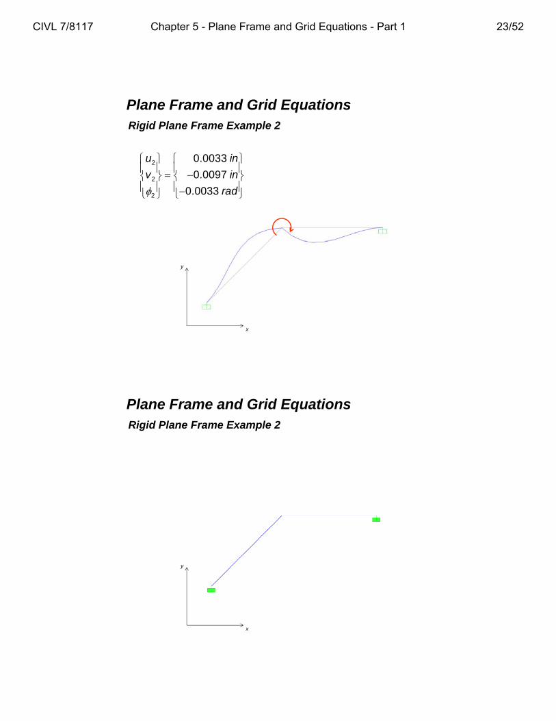
2
2
2
0.0033
0.0097
0.0033
u in
v in
rad
Nodal equivalent forces
CIVL 7/8117 Chapter 5 - Plane Frame and Grid Equations - Part 1 22/52
Plane Frame and Grid EquationsRigid Plane Frame Example 2
2
2
2
0.0033
0.0097
0.0033
u in
v in
rad
x
y
Plane Frame and Grid EquationsRigid Plane Frame Example 2
x
y
CIVL 7/8117 Chapter 5 - Plane Frame and Grid Equations - Part 1 23/52

0.707 0.707 0 0 0 0 0
0.707 0.707 0 0 0 0 0
0 0 1 0 0 0 0
0 0 0 0.707 0.707 0 0.0033
0 0 0 0.707 0.707 0 0.0097
0 0 0 0 0 1 0.0033
in
in
rad
Td
Plane Frame and Grid EquationsRigid Plane Frame Example 2
Element 1: The element force-displacement equations can be obtained using f’ = k’Td. Therefore, Td is:
0
0
0
0.00452
0.0092
0.0033
in
in
rad
Recall the elemental stiffness matrix is a function of values C1, C2, and L
6
2 33
30 10 (1,000)0.2273
12 30 2
kin
EIC
L
6
1
(100)30 105,893
12 30 2k
in
AEC
L
Plane Frame and Grid EquationsRigid Plane Frame Example 2
Element 1: The local force-displacement equations are:
Simplifying the above equations gives:
(1)
5,893 0 10 5,893 0 0 0
0 2.730 694.8 0 2.730 694.8 0
10 694.8 117,900 0 694.8 117,000 0
5,893 0 0 5,983 0 0 0.00452
0 2.730 694.8 0 2.730 694.8 0.0092
0 694.8 117,000 0 694.8 235,800 0.0033
in
in
rad
f k Td
1
1
1
2
2
2
26.64
2.268
389.1
26.64
2.268
778.2
x
y
x
y
f k
f k
m k in
f k
f k
m k in
CIVL 7/8117 Chapter 5 - Plane Frame and Grid Equations - Part 1 24/52

1 0 0 0 0 0 0.0033
0 1 0 0 0 0 0.0097
0 0 1 0 0 0 0.0033
0 0 0 1 0 0 0
0 0 0 0 1 0 0
0 0 0 0 0 1 0
in
in
rad
Td
Plane Frame and Grid EquationsRigid Plane Frame Example 2
Element 2: The element force-displacement equations can be obtained using f’ = k’Td. Therefore, Td is:
Recall the elemental stiffness matrix is a function of values C1, C2, and L
6
2 33
30 10 (1,000)0.2713
12 40k
in
EIC
L
6
1
(100)30 106,250
12 40k
in
AEC
L
0.0033
0.0097
0.0033
0
0
0
in
in
rad
Plane Frame and Grid EquationsRigid Plane Frame Example 2
Element 2: The local force-displacement equations are:
Simplifying the above equations gives:
20.63
2.58
832.57
20.63
2.58
412.50
k
k
k in
k
k
k in
k d
(2)
6,250 0 0 6,250 0 0 0.0033
0 3.25 781.1 0 3.25 781.1 0.0097
0 781.1 250,000 0 781.1 125,000 0.0033
6,250 0 0 6,250 0 0 0
0 3.25 781.1 0 3.25 781.1 0
0 781.1 125,000 0 781.1 250,00 0
in
in
rad
f k Td
CIVL 7/8117 Chapter 5 - Plane Frame and Grid Equations - Part 1 25/52

Plane Frame and Grid EquationsRigid Plane Frame Example 2
Element 2: To obtain the actual element local forces, we must subtract the equivalent nodal forces.
2
2
2
3
3
3
20.63 0
2.58 20
832.57 1600
20.63 0
2.58 20
412.50 1600
x
y
x
y
f k
f k k
m k in k in
f k
f k k
m k in k in
20.63
17.42
767.4
20.63
22.58
2,013
k
k
k in
k
k
k in
0 f kd f
Plane Frame and Grid EquationsRigid Plane Frame Example 2
The local forces in both elements are:
Element 2Element 1
CIVL 7/8117 Chapter 5 - Plane Frame and Grid Equations - Part 1 26/52
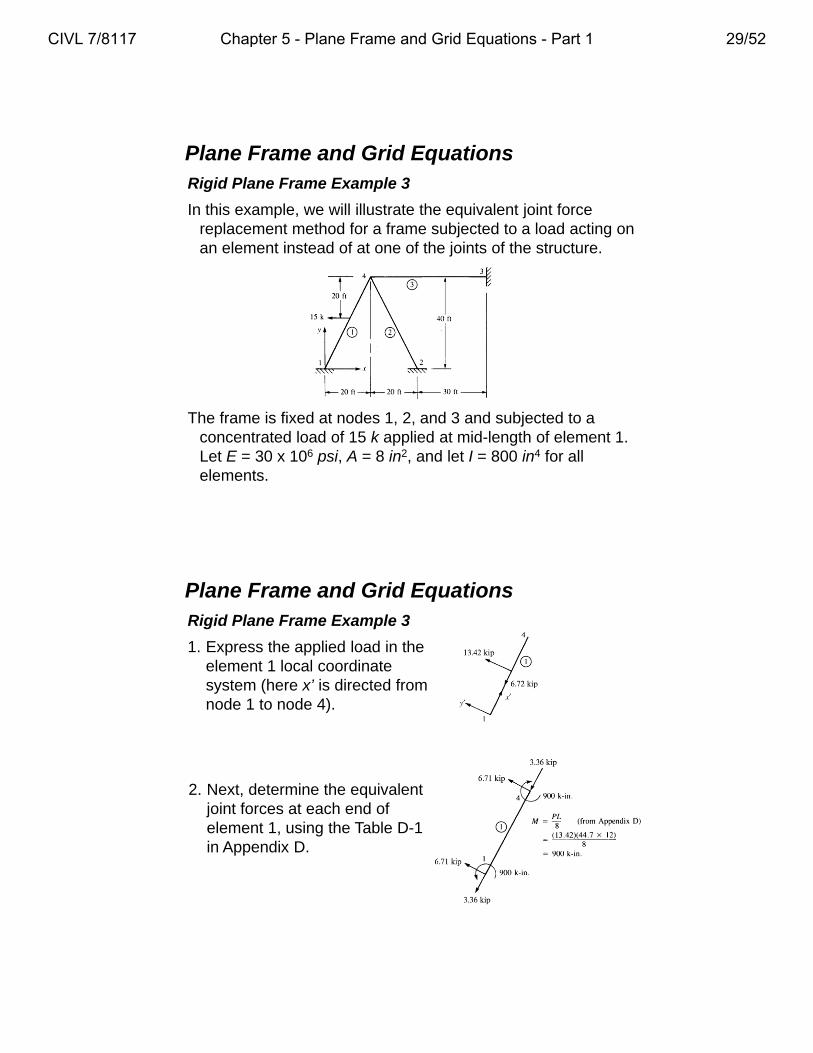
Plane Frame and Grid EquationsRigid Plane Frame Example 3
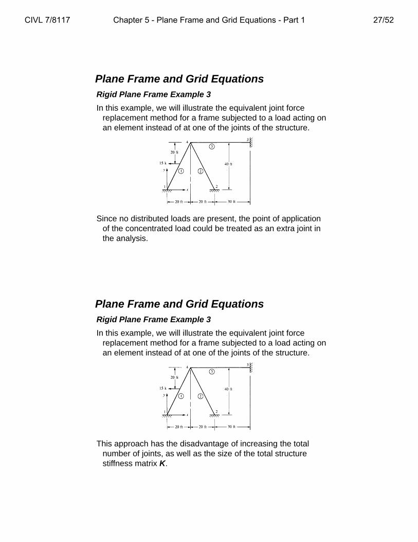
In this example, we will illustrate the equivalent joint force replacement method for a frame subjected to a load acting on an element instead of at one of the joints of the structure.
Since no distributed loads are present, the point of application of the concentrated load could be treated as an extra joint in the analysis.
Plane Frame and Grid EquationsRigid Plane Frame Example 3
In this example, we will illustrate the equivalent joint force replacement method for a frame subjected to a load acting on an element instead of at one of the joints of the structure.
This approach has the disadvantage of increasing the total number of joints, as well as the size of the total structure stiffness matrix K.
CIVL 7/8117 Chapter 5 - Plane Frame and Grid Equations - Part 1 27/52

Plane Frame and Grid EquationsRigid Plane Frame Example 3
In this example, we will illustrate the equivalent joint force replacement method for a frame subjected to a load acting on an element instead of at one of the joints of the structure.
For small structures solved by computer, this does not pose a problem.
Plane Frame and Grid EquationsRigid Plane Frame Example 3
In this example, we will illustrate the equivalent joint force replacement method for a frame subjected to a load acting on an element instead of at one of the joints of the structure.
However, for very large structures, this might reduce the maximum size of the structure that could be analyzed.
CIVL 7/8117 Chapter 5 - Plane Frame and Grid Equations - Part 1 28/52
Plane Frame and Grid EquationsRigid Plane Frame Example 3
In this example, we will illustrate the equivalent joint force replacement method for a frame subjected to a load acting on an element instead of at one of the joints of the structure.
The frame is fixed at nodes 1, 2, and 3 and subjected to a concentrated load of 15 k applied at mid-length of element 1. Let E = 30 x 106 psi, A = 8 in2, and let I = 800 in4 for all elements.
Plane Frame and Grid EquationsRigid Plane Frame Example 3
1. Express the applied load in the element 1 local coordinate system (here x’ is directed from node 1 to node 4).
2. Next, determine the equivalent joint forces at each end of element 1, using the Table D-1 in Appendix D.
CIVL 7/8117 Chapter 5 - Plane Frame and Grid Equations - Part 1 29/52

Plane Frame and Grid EquationsRigid Plane Frame Example 3
Plane Frame and Grid EquationsRigid Plane Frame Example 3
3. Then transform the equivalent joint forces from the local coordinate system forces into the global coordinate system forces, using the equation: f = TTf
These global joint forces are:
4. Then we analyze the structure, using the equivalent joint forces (plus actual joint forces, if any) in the usual manner.
5. The final internal forces developed at the ends of each element may be obtained by subtracting Step 2 joint forces from Step 4 joint forces.
CIVL 7/8117 Chapter 5 - Plane Frame and Grid Equations - Part 1 30/52

Plane Frame and Grid EquationsRigid Plane Frame Example 3
Element 1: The angle between x and x’ is 63.43º
0.447 0.895C S
36 6(800)8.95
12 44.7
Iin
L
6
3
30 1055.9
12 44.7
E kinL
4 4 4
(1)
90.0 178 448
178 359 244
448 244 179,000
u v
kin
k
2
22
12 12(800)0.0334
12 44.7
Iin
L
Plane Frame and Grid EquationsRigid Plane Frame Example 3
Element 2: The angle between x and x’ is 116.57º
0.447 0.895C S
36 6(800)8.95
12 44.7
Iin
L
6
3
30 1055.9
12 44.7
E kinL
4 4 4
(2)
90.0 178 448
178 359 244
448 244 179,000
u v
kin
k
2
22
12 12(800)0.0334
12 44.7
Iin
L
CIVL 7/8117 Chapter 5 - Plane Frame and Grid Equations - Part 1 31/52
Plane Frame and Grid EquationsRigid Plane Frame Example 3
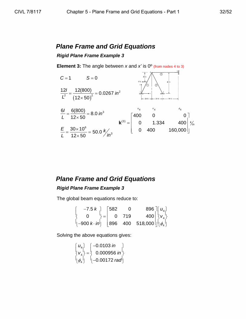
Element 3: The angle between x and x’ is 0º (from nodes 4 to 3)
1 0C S
36 6(800)8.0
12 50
Iin
L
6
3
30 1050.0
12 50
E kinL
4 4 4
(3)
400 0 0
0 1.334 400
0 400 160,000
u v
kin
k
2
22
12 12(800)0.0267
12 50
Iin
L
Plane Frame and Grid EquationsRigid Plane Frame Example 3
The global beam equations reduce to:
4
4
4
7.5 582 0 896
0 0 719 400
900 896 400 518,000
k u
v
k in
Solving the above equations gives:
4
4
4
0.0103
0.000956
0.00172
u in
v in
rad
CIVL 7/8117 Chapter 5 - Plane Frame and Grid Equations - Part 1 32/52

Plane Frame and Grid EquationsRigid Plane Frame Example 3
Element 1: The element force-displacement equations can be obtained using f’ = k’Td 0 0 0 0
0 0 0 0
0 0 1 0 0 0
0 0 0 0
0 0 0 0
0 0 0 0 0 1
C S
S C
C S
S C
T0.447 0.895C S
1
1
1
4
4
4
0.447 0.895 0 0 0 0
0.895 0.447 0 0 0 0
0 0 1 0 0 0
0 0 0 0.447 0.895 0
0 0 0 0.895 0.447 0
0 0 0 0 0 1
u
v
u
v
Td
0
0
0
0.00374
0.00963
0.00172
in
in
rad
0
0
0
0.0103
0.000956
0.00172
in
in
rad
Plane Frame and Grid EquationsRigid Plane Frame Example 3
Element 1: Recall the elemental stiffness matrix is:
1 1
2 2 2 22 2
2 2 2 2
1 1
2 2 2 22 2
2 2 2 2
0 0 0 0
0 12 6 0 12 6
0 6 4 0 6 2
0 0 0 0
0 12 6 0 12 6
0 6 2 0 6 4
C C
C LC C LC
LC C L LC C L
C C
C LC C LC
LC C L LC C L
k
6
1
(8)30 10447.2
12 44.72k
in
AEC
L
6
2 33
30 10 (800)0.155
12 44.72k
in
EIC
L
CIVL 7/8117 Chapter 5 - Plane Frame and Grid Equations - Part 1 33/52

Plane Frame and Grid EquationsRigid Plane Frame Example 3
Element 1: The local force-displacement equations are:
(1)
447 0 0 447 0 0 0
0 1.868 500.5 0 1.868 500.5 0
0 500.5 179,000 0 500.5 89,490 0
447 0 0 447 0 0 0.00374
0 1.868 500.5 0 1.868 500.5 0.00963
0 500.5 89,490 0 500.5 179,000 0.00172
in
in
rad
f k Td
(1)
1.67
0.88
158
1.67
0.88
311
k
k
k in
k
k
k in
f k d
(1)k Td
Plane Frame and Grid EquationsRigid Plane Frame Example 3
Element 1: To obtain the actual element local forces, we must subtract the equivalent nodal forces.
1
1
1
4
4
4
1.67 3.36
0.88 6.71
158 900
1.67 3.36
0.88 6.71
311 900
x
y
x
y
f k k
f k k
m k in k in
f k k
f k k
m k in k in
0 f kd f
5.03
7.59
1,058
1.68
5.83
589
k
k
k in
k
k
k in
CIVL 7/8117 Chapter 5 - Plane Frame and Grid Equations - Part 1 34/52

Plane Frame and Grid EquationsRigid Plane Frame Example 3
Element 2: The element force-displacement equations can be obtained using f’ = k’Td 0 0 0 0
0 0 0 0
0 0 1 0 0 0
0 0 0 0
0 0 0 0
0 0 0 0 0 1
C S
S C
C S
S C
T0.447 0.895C S
2
2
2
4
4
4
0.447 0.895 0 0 0 0
0.895 0.447 0 0 0 0
0 0 1 0 0 0
0 0 0 0.447 0.895 0
0 0 0 0.895 0.447 0
0 0 0 0 0 1
u
v
u
v
Td
0
0
0
0.00546
0.00879
0.00172
in
in
rad
0
0
0
0.0103
0.000956
0.00172
in
in
rad
Plane Frame and Grid EquationsRigid Plane Frame Example 3
Element 2: Recall the elemental stiffness matrix is:
1 1
2 2 2 22 2
2 2 2 2
1 1
2 2 2 22 2
2 2 2 2
0 0 0 0
0 12 6 0 12 6
0 6 4 0 6 2
0 0 0 0
0 12 6 0 12 6
0 6 2 0 6 4
C C
C LC C LC
LC C L LC C L
C C
C LC C LC
LC C L LC C L
k
6
1
(8)30 10447.2
12 44.72k
in
AEC
L
6
2 33
30 10 (800)0.155
12 44.72k
in
EIC
L
CIVL 7/8117 Chapter 5 - Plane Frame and Grid Equations - Part 1 35/52
Plane Frame and Grid EquationsRigid Plane Frame Example 3
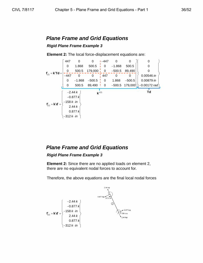
Element 2: The local force-displacement equations are:
(2)
447 0 0 447 0 0 0
0 1.868 500.5 0 1.868 500.5 0
0 500.5 179,000 0 500.5 89,490 0
447 0 0 447 0 0 0.00546
0 1.868 500.5 0 1.868 500.5 0.00879
0 500.5 89,490 0 500.5 179,000 0.00172
in
in
rad
f k Td
(2)
2.44
0.877
158
2.44
0.877
312
k
k
k in
k
k
k in
f k d
(2)k Td
Plane Frame and Grid EquationsRigid Plane Frame Example 3
Element 2: Since there are no applied loads on element 2, there are no equivalent nodal forces to account for.
Therefore, the above equations are the final local nodal forces
(2)
2.44
0.877
158
2.44
0.877
312
k
k
k in
k
k
k in
f k d
CIVL 7/8117 Chapter 5 - Plane Frame and Grid Equations - Part 1 36/52

Plane Frame and Grid EquationsRigid Plane Frame Example 3
Element 3: The element force-displacement equations can be obtained using f’ = k’Td 0 0 0 0
0 0 0 0
0 0 1 0 0 0
0 0 0 0
0 0 0 0
0 0 0 0 0 1
C S
S C
C S
S C
T1 0C S
4
4
4
3
3
3
1 0 0 0 0 0
0 1 0 0 0 0
0 0 1 0 0 0
0 0 0 1 0 0
0 0 0 0 1 0
0 0 0 0 0 1
u
v
u
v
Td
0.0103
0.000956
0.00172
0
0
0
in
in
rad
0.0103
0.000956
0.00172
0
0
0
in
in
rad
Plane Frame and Grid EquationsRigid Plane Frame Example 3
Element 3: Recall the elemental stiffness matrix is:
1 1
2 2 2 22 2
2 2 2 2
1 1
2 2 2 22 2
2 2 2 2
0 0 0 0
0 12 6 0 12 6
0 6 4 0 6 2
0 0 0 0
0 12 6 0 12 6
0 6 2 0 6 4
C C
C LC C LC
LC C L LC C L
C C
C LC C LC
LC C L LC C L
k
6
1
(8)30 10400
12 50k
in
AEC
L
6
2 33
30 10 (800)0.111
12 50k
in
EIC
L
CIVL 7/8117 Chapter 5 - Plane Frame and Grid Equations - Part 1 37/52

Plane Frame and Grid EquationsRigid Plane Frame Example 3
Element 3: The local force-displacement equations are:
(3)
400 0 0 400 0 0 0.0103
0 1.335 400 0 1.335 400 0.000956
0 400 160,000 0 400 80,000 0.00172
400 0 0 400 0 0 0
0 1.335 400 0 1.335 400 0
0 400 80,000 0 400 160,000 0
in
in
rad
f k Td
(3)
4.12
0.687
275
4.12
0.687
137
k
k
k in
k
k
k in
f k d
(3)k Td
Plane Frame and Grid EquationsRigid Plane Frame Example 3
Element 3: Since there are no applied loads on element 3, there are no equivalent nodal forces to account for.
Therefore, the above equations are the final local nodal forces
CIVL 7/8117 Chapter 5 - Plane Frame and Grid Equations - Part 1 38/52

Plane Frame and Grid EquationsRigid Plane Frame Example 4
The frame shown below is fixed at nodes 2 and 3 and subjected to a concentrated load of 500 kN applied at node 1.
For the bar, A = 1 x 10⁻³ m2, for the beam, A = 2 x 10⁻³ m2, I = 5 x 10⁻⁵ m4, and L = 3 m. Let E = 210 GPa for both elements.
Bar
Beam
Plane Frame and Grid EquationsRigid Plane Frame Example 4
Element 1: The angle between x and x’ is 0º
1 0C S
54 36 6(5 10 )
103
Im
L
66 3210 10
70 10 /3
EkN m
L
(1) 3
1 1 1
2 0 0
70 10 0 0.067 0.10
0 0.10 0.20
u v
kNm
k
55 2
2 2
12 12(5 10 )6.67 10
(3)
Im
L
CIVL 7/8117 Chapter 5 - Plane Frame and Grid Equations - Part 1 39/52

Plane Frame and Grid EquationsRigid Plane Frame Example 4
Element 2: The angle between x and x’ is 45º
0.707 0.707C S
2
1 1
3 2 6
(2)10 210 10 0.5 0.5
4.24 0.5 0.5
kNm kN
m
u v
m
m
k
1 1
(2) 3 0.354 0.35470 10
0.354 0.354kN
m
u v
k
Plane Frame and Grid EquationsRigid Plane Frame Example 4
Assembling the elemental stiffness matrices we obtain the global stiffness matrix:
3
2.354 0.354 0
70 10 0.354 0.421 0.10
0 0.10 0.20
kNm
K
The global equations are:
13
1
1
0 2.354 0.354 0
500 70 10 0.354 0.421 0.10
0 0 0.10 0.20
kNm
u
kN v
CIVL 7/8117 Chapter 5 - Plane Frame and Grid Equations - Part 1 40/52
Plane Frame and Grid EquationsRigid Plane Frame Example 4
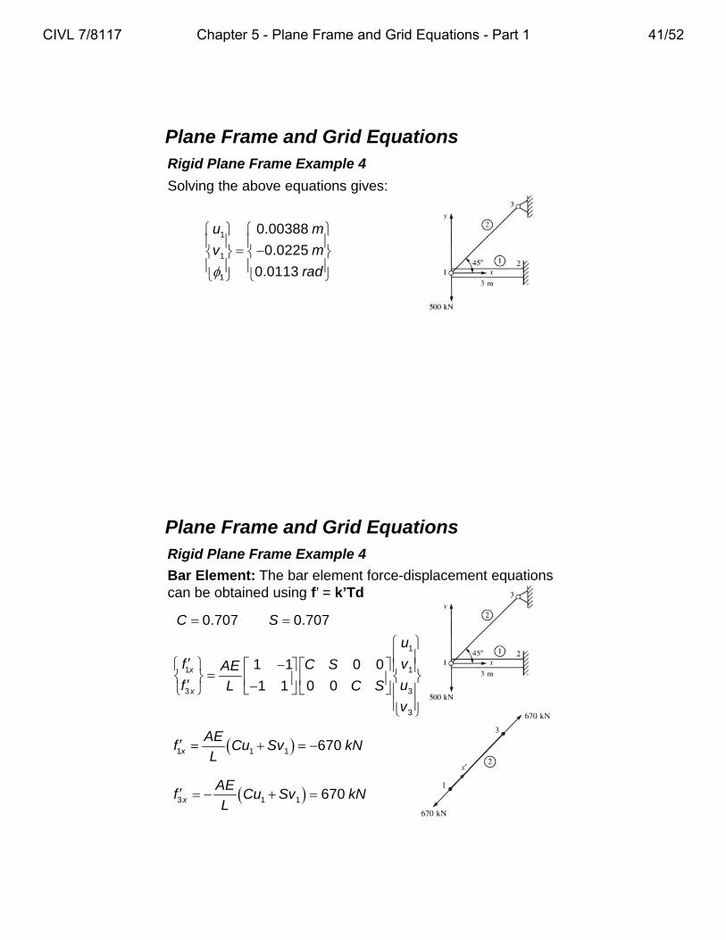
Solving the above equations gives:
1
1
1
0.00388
0.0225
0.0113
u m
v m
rad
Plane Frame and Grid EquationsRigid Plane Frame Example 4
Bar Element: The bar element force-displacement equations can be obtained using f’ = k’Td
0.707 0.707C S
1
1 1
3 3
3
1 1 0 0
1 1 0 0x
x
u
f vC SAEf uL C S
v
1 1 1 670x
AEf Cu Sv kN
L
3 1 1 670x
AEf Cu Sv kN
L
CIVL 7/8117 Chapter 5 - Plane Frame and Grid Equations - Part 1 41/52

Plane Frame and Grid EquationsRigid Plane Frame Example 4
0 0 0 0
0 0 0 0
0 0 1 0 0 0
0 0 0 0
0 0 0 0
0 0 0 0 0 1
C S
S C
C S
S C
T
1
0
C
S
1
1
1
2
2
2
1 0 0 0 0 0
0 1 0 0 0 0
0 0 1 0 0 0
0 0 0 1 0 0
0 0 0 0 1 0
0 0 0 0 0 1
u
v
u
v
d Td
0.00388
0.0225
0.0113
0
0
0
m
m
rad
0.00388
0.0225
0.0113
0
0
0
m
m
rad
Beam Element: The bar element force-displacement equations can be obtained using f’ = k’Td
Plane Frame and Grid EquationsRigid Plane Frame Example 4
Beam Element: The bar element force-displacement equations can be obtained using f’ = k’Td
1 1
2 2 2 22 2
2 2 2 2
1 1
2 2 2 22 2
2 2 2 2
0 0 0 0
0 12 6 0 12 6
0 6 4 0 6 2
0 0 0 0
0 12 6 0 12 6
0 6 2 0 6 4
C C
C LC C LC
LC C L LC C L
C C
C LC C LC
LC C L LC C L
k
63
1
(0.002)210 10140 10
3kN
m
AEC
L
6 5
2 33
210 10 (5 10 )388.89
3kN
m
EIC
L
CIVL 7/8117 Chapter 5 - Plane Frame and Grid Equations - Part 1 42/52

Plane Frame and Grid EquationsRigid Plane Frame Example 4
Beam Element: The bar element force-displacement equations can be obtained using f’ = k’Td
3(1)
2 0 0 2 0 0 0.00388
0 0.067 0.10 0 0.067 0.10 0.0225
0 0.10 0.20 0 0.10 0.10 0.011370 10
2 0 0 2 0 0 0
0 0.067 0.10 0 0.067 0.10 0
0 0.10 0.10 0 0.10 0.20 0
m
m
kN m
f k d
1
1
1(1)
2
2
2
473
26.5
0.0
473
26.5
78.3
x
y
x
y
f kN
f kN
m
f kN
f kN
m kN m
f
(1)k d
Plane Frame and Grid EquationsRigid Plane Frame Example 4
CIVL 7/8117 Chapter 5 - Plane Frame and Grid Equations - Part 1 43/52

Plane Frame and Grid EquationsRigid Plane Frame Example 5
The frame is fixed at nodes 1 and 3 and subjected to a moment of 20 kN-m applied at node 2
Assume A = 2 x 10⁻² m2, I = 2 x 10⁻⁴ m4, and E = 210 GPa for all elements.
Plane Frame and Grid EquationsRigid Plane Frame Example 5
Element 1: The angle between x and x’ is 90º
0 1C S
44 36 6(2 10 )
3 104
Im
L
3
67210 10
5.25 104
kNm
E
L
2 2 2
(1) 5
0.015 0 0.03
5.25 10 0 2 0
0.03 0 0.08
u v
kNm
k
44 2
2 2
12 12(2 10 )1.5 10
(4)
Im
L
The parts of k associated with node 2 are:
CIVL 7/8117 Chapter 5 - Plane Frame and Grid Equations - Part 1 44/52

Plane Frame and Grid EquationsRigid Plane Frame Example 5
Element 2: The angle between x and x’ is 0º
1 0C S
44 36 6(2 10 )
2.4 105
Im
L
3
67210 10
4.2 105
kNm
E
L
2 2 2
(2) 5
2 0 0
4.2 10 0 0.0096 0.024
0 0.024 0.08
u v
kNm
k
44 2
2 2
12 12(2 10 )9.6 10
(5)
Im
L
The parts of k associated with node 2 are:
Plane Frame and Grid EquationsRigid Plane Frame Example 5
Assembling the elemental stiffness matrices we obtain the global stiffness matrix:
6
0.8480 0 0.0158
10 0 1.0500 0.0101
0.0158 0.0101 0.0756
kNm
K
The global equations are:
26
2
2
0 0.8480 0 0.0158
0 10 0 1.0500 0.0101
20 0.0158 0.0101 0.0756
u
v
kN m
CIVL 7/8117 Chapter 5 - Plane Frame and Grid Equations - Part 1 45/52

Plane Frame and Grid EquationsRigid Plane Frame Example 5
Solving the above equations gives:
62
62
42
4.95 10
2.56 10
2.66 10
u m
v m
rad
Plane Frame and Grid EquationsRigid Plane Frame Example 5
0 0 0 0
0 0 0 0
0 0 1 0 0 0
0 0 0 0
0 0 0 0
0 0 0 0 0 1
C S
S C
C S
S C
T
0
1
C
S
1
1
1
2
2
2
0 1 0 0 0 0
1 0 0 0 0 0
0 0 1 0 0 0
0 0 0 0 1 0
0 0 0 1 0 0
0 0 0 0 0 1
u
v
u
v
d Td6
6
4
0
0
0
2.56 10
4.95 10
2.66 10
m
m
rad
6
6
4
0
0
0
4.95 10
2.56 10
2.66 10
m
m
rad
Element 1: The element force-displacement equations can be obtained using f’ = k’Td
CIVL 7/8117 Chapter 5 - Plane Frame and Grid Equations - Part 1 46/52

Plane Frame and Grid EquationsRigid Plane Frame Example 5
1 1
2 2 2 22 2
2 2 2 2
1 1
2 2 2 22 2
2 2 2 2
0 0 0 0
0 12 6 0 12 6
0 6 4 0 6 2
0 0 0 0
0 12 6 0 12 6
0 6 2 0 6 4
C C
C LC C LC
LC C L LC C L
C C
C LC C LC
LC C L LC C L
k
2 66
1
(2 10 )210 101.05 10
4kN
m
AEC
L
6 5
2 33
210 10 (5 10 )388.89
3kN
m
EIC
L
Element 1: The element force-displacement equations can be obtained using f’ = k’Td
Plane Frame and Grid EquationsRigid Plane Frame Example 5
3(1) 6
6
4
200 0 0 200 0 0 0
0 1.5 3 0 1.5 3 0
0 3 8 0 3 4 05.25 10
200 0 0 200 0 0 2.56 10
0 1.5 3 0 1.5 3 4.95 10
0 3 4 0 3 8 2.66 10
m
m
rad
f k d
1
1
1(1)
2
2
2
2.69
4.2
5.59
2.69
4.2
11.17
x
y
x
y
f kN
f kN
m kN m
f kN
f kN
m kN m
f
Element 1: The element force-displacement equations can be obtained using f’ = k’Td
(1)k d
CIVL 7/8117 Chapter 5 - Plane Frame and Grid Equations - Part 1 47/52

Plane Frame and Grid EquationsRigid Plane Frame Example 5
0 0 0 0
0 0 0 0
0 0 1 0 0 0
0 0 0 0
0 0 0 0
0 0 0 0 0 1
C S
S C
C S
S C
T1
0
C
S
2
2
2
3
3
3
1 0 0 0 0 0
0 1 0 0 0 0
0 0 1 0 0 0
0 0 0 1 0 0
0 0 0 0 1 0
0 0 0 0 0 1
u
v
u
v
d Td
6
6
4
4.95 10
2.56 10
2.66 10
0
0
0
m
m
rad
6
6
4
4.95 10
2.56 10
2.66 10
0
0
0
m
m
rad
Element 2: The element force-displacement equations can be obtained using f’ = k’Td
Plane Frame and Grid EquationsRigid Plane Frame Example 5
1 1
2 2 2 22 2
2 2 2 2
1 1
2 2 2 22 2
2 2 2 2
0 0 0 0
0 12 6 0 12 6
0 6 4 0 6 2
0 0 0 0
0 12 6 0 12 6
0 6 2 0 6 4
C C
C LC C LC
LC C L LC C L
C C
C LC C LC
LC C L LC C L
k
2 66
1
(2 10 )210 100.84 10
5kN
m
AEC
L
6 4
2 33
210 10 (2 10 )336
5kN
m
EIC
L
Element 2: The element force-displacement equations can be obtained using f’ = k’Td
CIVL 7/8117 Chapter 5 - Plane Frame and Grid Equations - Part 1 48/52

Plane Frame and Grid EquationsRigid Plane Frame Example 5
6
6
43
(2)
200 0 0 200 0 0 4.95 10
0 0.96 2.40 0 0.96 2.40 2.56 10
0 2.40 8 0 2.40 4 2.66 104.2 10
200 0 0 200 0 0 0
0 0.96 2.40 0 0.96 2.40 0
0 2.40 4 0 2.40 8 0
m
m
rad
f k d
2
2
2(2)
3
3
3
4.16
2.69
8.92
4.16
2.69
4.47
x
y
x
y
f kN
f kN
m kN m
f kN
f kN
m kN m
f
Element 2: The element force-displacement equations can be obtained using f’ = k’Td
(2)k d
Plane Frame and Grid EquationsInclined or Skewed Supports
If a support is inclined, or skewed, at some angle for the global x axis, as shown below.
The boundary conditions on the displacements are not in the global x-y directions but in the x’-y’ directions.
CIVL 7/8117 Chapter 5 - Plane Frame and Grid Equations - Part 1 49/52

Plane Frame and Grid EquationsInclined or Skewed Supports
We must transform the local boundary condition of v’3 = 0 (in local coordinates) into the global x-y system.
Plane Frame and Grid EquationsInclined or Skewed Supports
Therefore, the relationship between of the components of the displacement in the local and the global coordinate systems at node 3 is:
3 3
3 3
3 3
' cos sin 0
' sin cos 0
' 0 0 1
u u
v v
We can rewrite the above expression as:
3
cos sin 0
sin cos 0
0 0 1
t
3 3 3' [ ]d t d
CIVL 7/8117 Chapter 5 - Plane Frame and Grid Equations - Part 1 50/52

Plane Frame and Grid EquationsInclined or Skewed Supports
We can apply this sort of transformation to the entire displacement vector as:
where the matrix [Ti] is:
' [ ] or [ ] 'Ti id T d d T d
3
[ ] [0] [0]
[ ] [0] [ ] [0]
[0] [0] [ ]i
I
T I
t
Both the identity matrix [I] and the matrix [t3] are 3 x 3 matrices.
Plane Frame and Grid EquationsInclined or Skewed Supports
The force vector can be transformed by using the same transformation.
In global coordinates, the force-displacement equations are:
' [ ]if T f
By using the relationship between the local and the global displacements, the force-displacement equations become:
[ ]f K d
[ ] [ ][ ]i iT f T K d
Applying the skewed support transformation to both sides of the force-displacement equation gives:
[ ] [ ][ ][ ] ' ' [ ][ ][ ] 'T Ti i i i iT f T K T d f T K T d
CIVL 7/8117 Chapter 5 - Plane Frame and Grid Equations - Part 1 51/52

Plane Frame and Grid EquationsInclined or Skewed Supports
Therefore the global equations become:
1 1
1 1
1 1
2 2
2 2
2 2
3 3
3 3
3 3
[ ][ ][ ]
' '
' '
x
y
xT
i iy
x
y
F u
F v
M
F u
T K TF v
M
F u
F v
M
Elemental coordinates
End of Chapter 5a
CIVL 7/8117 Chapter 5 - Plane Frame and Grid Equations - Part 1 52/52