planetary magnetic fields and fluid dynamosrs/res/b/planetdyn/jones2011.pdf · ·...

FL43CH24-Jones ARI 15 November 2010 14:28

Planetary Magnetic Fieldsand Fluid DynamosChris A. JonesDepartment of Applied Mathematics, University of Leeds, Leeds LS2 9JT, United Kingdom;email: [email protected]

Annu. Rev. Fluid Mech. 2011. 43:583–614

First published online as a Review in Advance onSeptember 22, 2010

The Annual Review of Fluid Mechanics is online atfluid.annualreviews.org

This article’s doi:10.1146/annurev-fluid-122109-160727

Copyright c© 2011 by Annual Reviews.All rights reserved

0066-4189/11/0115-0583$20.00

Keywords

geomagnetism, dynamo theory, dynamo simulations, planetary cores

Abstract

The magnetic fields of the planets, including the Earth, are generated bydynamo action in their fluid cores. Numerical models of this process havebeen developed that solve the fundamental magnetohydrodynamic equationsdriven by convection in a rotating spherical shell. New results from thesetheoretical models are compared with observations of the geomagnetic fieldand magnetic data gathered from space missions. The mechanism by whicha magnetic field is created is examined. The effects of rotation and magneticfield on the convection are of paramount importance in the simulations. Awide range of simulations with different convection models, varying bound-ary conditions, and parameter values have been performed over the past10 years. The effects of these differences are assessed. Numerical consider-ations mean that all dynamo simulations use much enhanced values of thediffusivities. We consider to what extent this affects results and show howthe asymptotic behavior at low diffusion is starting to be inferred using scal-ing laws. The results of specific models relating to individual planets arereviewed.

583

Ann

u. R

ev. F

luid

Mec

h. 2

011.

43:5

83-6

14. D

ownl

oade

d fr

om w

ww

.ann

ualr

evie

ws.

org

by G

lasg

ow U

nive

rsity

on

11/0

2/13

. For

per

sona

l use

onl

y.


1. INTRODUCTION

A series of space missions over the past 40 years has greatly enhanced our knowledge of themagnetic fields of the planets in our solar system, and also the magnetic fields of the largersatellites, which here we count as planets. We focus on the internal magnetic fields of the planets,so the active research topics of planetary magnetospheres and their interaction with the solar windare not discussed here. The picture that has emerged is a remarkably complex one, with someplanets having strong internal magnetic fields, and others having no discernible field in their core.There is evidence that Mars had a strong internal field in the past, but it does not have one atpresent.

It is generally believed that the internal magnetic fields are generated by dynamo action; thatis, the field is created by fluid motion in planetary cores. Larmor (1919) suggested this possibilitymainly in connection with the magnetic fields of sunspots, and Elsasser (1939) and Bullard (1949)gave the theoretical basis for the modern ideas of convection-driven dynamos. The temperature inplanetary cores is well above the Curie temperature, so permanent magnetism cannot occur. In theabsence of fluid motion, the Earth’s magnetic field strength would decay by a factor e approximatelyevery 15,000 years (see, e.g., Moffatt 1978), leaving a negligible field over the Earth’s lifetime,4.5 billion years. Many possibilities for generating planetary magnetic fields (e.g., the thermoelec-tric effect, magnetic monopoles) have been proposed, but all either have no reliable physical basisor have been shown to produce fields much smaller than those observed (Stevenson 2007).

Although Larmor’s dynamo hypothesis has been generally accepted, the question of what isdriving the fluid motion, and supplying the energy that is being lost to ohmic heating in planetarycores, is much more controversial. The most popular idea is that the dynamo is powered bythermal and compositional convection in the fluid core. In the case of the Earth, this means thefluid outer part of the core. Others have suggested that precession or tidal interactions mightdrive the dynamo (see, e.g., Malkus 1994, Tilgner 2007a), in which case the planet’s rotation isthe ultimate energy source for the magnetic field (see Tilgner 2007b for a review of the rotationaldynamics of the Earth’s core). In this review we concentrate on convection-driven dynamos, partlybecause their theory is much more developed than the theory of precession-driven dynamos, andpartly because simple estimates suggest that convection can produce flows of the necessary orderof magnitude, and the flows produced can be shown to give rise to dynamo action.

In parallel with the space exploration of planetary magnetism, considerable theoretical progresshas been made in our understanding of convection-driven dynamos in spherical shells. This hasbeen driven largely by the remarkable improvements in high-performance computers, which allowthree-dimensional simulations in which the Navier-Stokes and induction equations are solvedsimultaneously. This only became feasible in the 1990s, but much progress has been made sincethen. Our understanding of planetary dynamos is more advanced than our understanding of stellardynamos, because the magnetic Reynolds number, Rm, in planets is generally moderate, and theinduction equation is therefore numerically tractable. There are serious theoretical difficulties withnonlinear dynamos in the high Rm limit, which emerged in the 1990s and which have not yet beenfully resolved (see, e.g., Hughes 2007). There are nevertheless problems with current planetarydynamo simulations (see, e.g., Jones 2000), because two small parameters, the Ekman numberand the magnetic Prandtl number, appear in the fundamental equations. Dynamo simulationscannot reach the very small values of these parameters that are found in planetary cores, and sowe still need to understand the limiting behavior of the models as these parameters become small,which remains a challenging problem. There have been some important theoretical advances inour understanding of convection in the presence of rotation and magnetic field that have helpedthe interpretation of the results emerging from the very complex simulations. There are also a

584 Jones

Ann

u. R

ev. F

luid

Mec

h. 2

011.

43:5

83-6

14. D

ownl

oade

d fr

om w

ww

.ann

ualr

evie

ws.

org

by G

lasg

ow U

nive

rsity

on

11/0

2/13

. For

per

sona

l use

onl

y.


number of laboratory dynamo and magnetohydrodynamic experiments, which also cannot reachthe planetary regime, but nevertheless do probe a different part of the parameter space, whichhelps to build up understanding.

The planets are conveniently divided into three groups (Stevenson 2003): the terrestrial planetswith rocky interiors, some of which have fluid cores; the gas giants Jupiter and Saturn, whosecomposition is primarily hydrogen and helium; and the ice giants, Uranus and Neptune, whichhave deep gaseous atmospheres but also have more heavy elements than in solar composition.Far more is known about the Earth than the other planets, because the observation history islonger and more accurate, and seismology gives us detailed information about the nature of thecore. Three terrestrial planets have magnetic fields strong enough to suggest an internal field andtherefore a dynamo: the Earth, Mercury, and Ganymede, the largest moon of Jupiter. The strongremanent magnetism of Mars, discovered by the Global Surveyor mission (Acuna et al. 1999),suggests that Mars once had a dynamo but that it ceased to operate probably about 350 millionyears after the planet’s birth. Venus has no measurable internal field. Our Moon has patches ofcrustal magnetization, which may be remnants of an era when the Moon had a working dynamo,but it is also possible that lunar magnetic fields were created during meteorite impacts (Stevenson2003). None of the other larger satellites in the solar system have strong internal fields, althoughthere are induction effects in the inner Jovian satellites due to their motion through Jupiter’smagnetic field.

Previous review articles relating to this material are Busse (2000), which discusses the thenexisting laboratory experiments and spherical convection-driven dynamo models; Kono & Roberts(2002), which covers the geomagnetic field and its relation to dynamo simulations; and Jones (2003,2007a), which review magnetic fields in planets. Christensen & Wicht (2007) focused on numericaldynamo simulations, and Jones (2007b) addressed thermal and compositional convection in thecore.

2. THE GEOMAGNETIC FIELD

Magnetic fields generated internally can be represented in the electrically insulating region abovethe core by the spherical harmonic expansion for the potential

� = rs

∞∑n=1

m=n∑m=0

(rs

r

)n+1Pm

n (cos θ )(gmn cos mφ + hm

n sin mφ), (1)

where the magnetic field B = −∇�, and r, θ , and φ are spherical polar coordinates, with θ as thecolatitude. Here the associated Legendre polynomials have the partial Schmidt normalization (see,e.g., Merrill et al. 1996, p. 28), and the coefficients gm

n and hmn are the Gauss coefficients. Planetary

magnetic fields, including that of the Earth, are usually specified by their Gauss coefficients.Equation 1 can be used to reconstruct the field either at the planetary surface r = rs or at thecore-mantle boundary (CMB), r = rcmb = 3.48 × 106 m for the Earth.

2.1. The Magnetic Field Spectrum

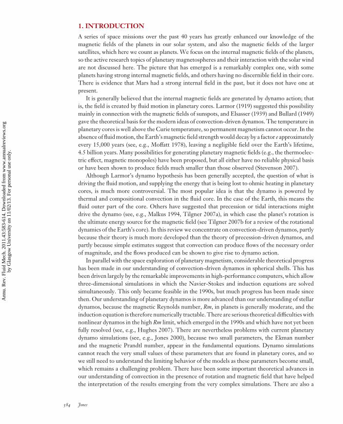
Figure 1a shows the radial component of the Earth’s field at the surface. Note that the axial dipoleg0

1 component dominates the picture. Figure 1b shows the field at the CMB. It is still essentiallydipolar, but the field clearly has much more small-scale structure, as well as being about 10 timesstronger. Also of interest in Figure 1b is the large reversed field patch in the South Atlantic. Thisfeature has been growing over the past few 100 years, which is the main reason why the dipole

www.annualreviews.org • Planetary Magnetic Fields and Fluid Dynamos 585

Ann

u. R

ev. F

luid

Mec

h. 2

011.

43:5

83-6

14. D

ownl

oade

d fr

om w

ww

.ann

ualr

evie

ws.

org

by G

lasg

ow U

nive

rsity

on

11/0

2/13

. For

per

sona

l use

onl

y.


+0.1 mT –0.1 mT

+1 mT –1 mT

a

b

Radial magnetic field


Figure 1(a) The radial component of the Earth’s magnetic field at the surface and (b) at the core-mantle boundary,both using the Hammer-Aitoff projection. In panel b, shorter wavelengths may be present in the true field,but they have to be filtered out because of crustal-field contamination. Figure provided by R. Holme.

component of the geomagnetic field is in decline (Gubbins et al. 2006). The relative content ofhigher harmonics is measured by the Lowes-Mauersberger spectrum

Rn =(rs

r

)2n+4(n + 1)

n∑m=0

[(gmn )2 + (hm

n )2], (2)

which is fairly constant with n up to degree about 12 if r is evaluated at the CMB (see, e.g., Mauset al. 2005). For higher n, the geomagnetic core field is obscured by crustal magnetism. Thespectrum must tail off at some value of n > 12 because otherwise the ohmic dissipation would betoo large. A recent discussion of bounds on the ohmic heat dissipation for the geomagnetic fieldis given by Jackson & Livermore (2009). Another interesting feature of Figure 1b is the stringof flux patches just south of the equator from the mid-Atlantic, which are propagating westward( Jackson 2003). The time dependence, called the secular variation, is measured by continuousmonitoring of the field by satellites and magnetic observatories.

586 Jones

Ann

u. R

ev. F

luid

Mec

h. 2

011.

43:5

83-6

14. D

ownl

oade

d fr

om w

ww

.ann

ualr

evie

ws.

org

by G

lasg

ow U

nive

rsity

on

11/0

2/13

. For

per

sona

l use

onl

y.


20.0 km year–1

Figure 2Core flow inferred from secular variation observations using the tangential geostrophy assumption. Figurereproduced with permission from Holme & Olsen (2006).

2.2. The Core Flow

The secular variation enables the velocity below the CMB to be reconstructed, provided someassumptions are accepted. The most common assumption is the frozen flux hypothesis (Roberts& Scott 1965),

∂ Br

∂t= −∇H · (uH Br ), (3)

where ∇H is the horizontal gradient, uH is the tangential flow just below the CMB, and Br

is the radial component of the magnetic field. As this is only one equation for two unknownvelocity components, an additional constraint from the equation of motion is required. A commonassumption is tangential geostrophy, which is ∇H · cos θuH = 0, although several others havebeen used (Holme 2007). Figure 2 shows the tangential components of u that result from theseassumptions (Holme & Olsen 2006). The most important deduction for dynamo theory is theestimate of the typical core velocity, which is consistent with that expected from thermal andcompositional convection in the core and is also capable of generating magnetic field by dynamoinduction (see below).

2.3. Reversals and Excursions

The geomagnetic field reverses polarity rather randomly. The reversal rate is typically once every0.3 Myr (see Merrill et al. 1996 for a full discussion), but reversals are completed relatively quickly,on a timescale of around 20,000 years only. There have been long periods, around 40 Myr, duringwhich the field has not reversed at all, the most famous being the Cretaceous superchron, 83–124 Myr before present. A rather controversial observation is that the dipole axis of the field haspreferred longitude paths during reversal (Hoffman 1992), discussed by Glatzmaier & Coe (2007).In addition to the full reversals, the dipole axis has much more frequent excursions (e.g., Valetet al. 2005), which may be thought of as failed reversals because the field strength drops and thedipolar component moves away from the geographical polar axis, but eventually the field recoversits original polarity.

3. DYNAMO MODELS

Dynamo simulations in spherical geometry have mostly used the Boussinesq approximation,although recently anelastic dynamo models have been developed. These have mostly been used


Ann

u. R

ev. F

luid

Mec

h. 2

011.

43:5

83-6

14. D

ownl

oade

d fr

om w

ww

.ann

ualr

evie

ws.

org

by G

lasg

ow U

nive

rsity

on

11/0

2/13

. For

per

sona

l use

onl

y.


g

Flux

Flux

Tangentcylinder

s

z

ΩCMB

ICB

Figure 3Geometry used for spherical shell geodynamo simulations. The fluid outer core lies between the inner-coreboundary (ICB) and core-mantle boundary (CMB). Gravity is directed radially inward, and the heat flux iscarried outward.

to investigate stellar dynamos, with the ASH (anelastic spherical harmonic) code (Clune et al.1999) perhaps the best-known code. Some work has been done on compressible models for thegiant planets ( Jones & Kuzanyan 2009), and more is in progress. The configuration used by theBoussinesq codes is shown in Figure 3. The fluid outer core lies between the inner-core boundary(ICB) and the CMB. The inner core is an electrically conducting solid, mostly iron. Spherical polarcoordinates r, θ , and φ are used in the computations, but cylindrical coordinates s, φ, and z arealso useful to discuss results. There is rotation � about the z axis, and gravity is radially inward,and of magnitude proportional to r, appropriate for a uniform sphere. Centrifugal acceleration isneglected. The unit of length is the gap width d = rcmb − ricb, and for the Earth ricb = 1.22 × 106 mand d = 2.26 × 106 m. The tangent cylinder, marked in Figure 3, is an imaginary cylinder, butit does divide the core into regions where the dynamical behavior is rather different.

We use the magnetic diffusion time d2/η as the unit of time, where η is the magnetic diffusivity,estimated at 2 m2 s−1 in metallic cores. The unit of velocity is then η/d, so the dimensionless velocityis a direct measure of the magnetic Reynolds number Rm = U∗d/η, where U∗ is the typical corevelocity. The unit of magnetic field is (�ρμη)1/2, where ρ is the density (∼104 kg m−3), andμ = 4π × 10−7 in SI units is the permeability of free space, so a magnetic field of strength 1has an Elsasser number = B2

0 /�ρμη of unity. In the Earth’s core this unit is about 1.4 mT or14 Gauss.

The dimensional Boussinesq equation of motion is

ρDuDt

+ 2ρ� × u = −∇ p + j × B + ρν∇2u + ρg0

rcmb(αT + ξ )r. (4)

Here u is the velocity, p is the pressure, ν is the kinematic viscosity, and j is the current density,which is ∇×B/μ by Ampere’s law. g0 is gravity at the CMB, and the buoyancy term has a thermalpart αT, where α is the coefficient of thermal expansion, and a compositional component ξ , whereξ is the mass fraction of light material (believed to be sulphur and oxygen in the Earth’s core).

588 Jones

Ann

u. R

ev. F

luid

Mec

h. 2

011.

43:5

83-6

14. D

ownl

oade

d fr

om w

ww

.ann

ualr

evie

ws.

org

by G

lasg

ow U

nive

rsity

on

11/0

2/13

. For

per

sona

l use

onl

y.


The dimensionless form isE

PmDuDt

+ 2z × u = −∇ p + (∇ × B) × B + E∇2u + Ra E PmPr

(T + ξ )r

rcmb. (5)

Here the unit of temperature is �T, the superadiabatic temperature difference across the core,and the unit of ξ is α�T.

The dimensionless induction equation is

∂B∂t

= ∇2B + ∇ × (u × B), (6)

and the temperature and composition equations are

∂T∂t

= PmPr

∇2T − u · ∇T + Q, (7)

and∂ξ

∂t= Pm

Pc∇2ξ − u · ∇ξ + Qξ , (8)

and we also have

∇ · B = ∇ · u = 0 (9)

for Boussinesq fluid.The dimensionless parameters are

Ra = g0α�T d 3

νκ, Pr = ν

κ, Pm = ν

η, Pc = ν

κξ

, E = ν

�d 2, (10)

where Ra is the Rayleigh number, Pr the Prandtl number, Pm the magnetic Prandtl number,Pc the compositional Prandtl number, and E the Ekman number. κ and κξ are the thermal andcompositional diffusivities, respectively. The terms Q and Qξ represent internal heating (or cool-ing) and internal compositional sources. To complete the model we must specify the radius ratioricb/rcmb, taken as 0.35 for the Earth’s core, and the boundary conditions. The usual estimate forthe molecular value of E is 10−15, way below what can be achieved numerically. Even if we supposea turbulent diffusion increasing the viscosity to the value of the magnetic diffusivity, and there isno compelling physical reason to assume so large a turbulent diffusion, we still have E ∼ 5×10−9,also below anything numerically possible. The fluid Prandtl number in metallic cores is typically0.1, and the compositional Prandtl number is large, but the magnetic Prandtl number is verysmall, of order 10−6. This is far below what can be achieved in simulations. It is often argued thatturbulence will enhance the effective values of the Prandtl numbers toward unity. This may wellbe the case, but our current understanding of the nature of core turbulence is very limited. Thepossible form of small-scale turbulence to be expected in the core and its effects are discussedby Braginsky & Meytlis (1990) and Braginsky & Roberts (1995). The very slow flows, the rapidrotation, and strong influence of the magnetic field mean that we are far from regimes that can bestudied experimentally or numerically.

To estimate the Rayleigh number inside the core, we need to know the superadiabatic temper-ature difference between the ICB and CMB. This is very much less than the actual temperaturedifference, which is of order 103 K, because the core is almost certainly very close to adiabaticstratification. In Section 6 below, we estimate the typical temperature fluctuation as having anorder of magnitude of 10−3 K. In practice, the Rayleigh number is often chosen so that a sensiblevalue of the magnetic Reynolds number is found.

Equations 5–10 form a complete set of equations, which together with appropriate boundaryconditions can be integrated forward in time. Another issue is the choice of heat and composition


Ann

u. R

ev. F

luid

Mec

h. 2

011.

43:5

83-6

14. D

ownl

oade

d fr

om w

ww

.ann

ualr

evie

ws.

org

by G

lasg

ow U

nive

rsity

on

11/0

2/13

. For

per

sona

l use

onl

y.


sources, Q and Qξ . As the inner core grows, the light-element composition increases, and this is aneffective uniform sink. Similarly, a gradual cooling of the core is an effective heat source. As moreheat is conducted down the adiabat near the CMB than near the ICB, heat flux is removed fromthe convection to appear as conduction, so this is an effective heat sink. These rather complicatedheat and composition source issues are discussed in detail in Anufriev et al. (2005).

In practice, not much attention has been paid to the case with both compositional and thermaldriving. If the Prandtl numbers are close to unity (as may be the case if turbulent diffusion dom-inates), and similar boundary conditions are used for temperature and composition, temperatureand composition may be combined into one codensity variable (Braginsky & Roberts 1995). Partlybecause of this, and for reasons of simplicity, most dynamo models have used only one buoyancysource, usually called temperature.

To interpret the solutions that emerge from integration of these equations, the linear theoryof rapidly rotating convection in spherical shells is essential. This linear theory is now fairlywell understood. Roberts (1968) and Busse (1970) established that convection onsets in tall thincolumns. Numerical solutions showing the columns spiralling outward in the s -φ plane were foundby Zhang (1992), and the full small E asymptotic theory was evaluated by Jones et al. (2000) andDormy et al. (2004). There is now excellent agreement between numerics and asymptotics, andthe theory has recently been extended to anelastic compressible convection by Jones et al. (2009).

The first time-dependent numerical solutions of the full magnetohydrodynamic equationsgiven in Equations 5–10 in spherical geometry appeared in the mid-1990s (Glatzmaier & Roberts1995, 1996a,b, 1997; Jones et al. 1995; Kageyama et al. 1995; Kuang & Bloxham 1997). It soonbecame apparent that steady dipolar dynamos, and dynamos that occasionally reversed, werepossible. The flow speeds generating the fields give magnetic Reynolds numbers similar to thoseindicated by the core flow measurement techniques of Section 2.2.

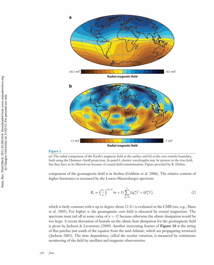
Many different boundary conditions have been used, and the effects of different boundaryconditions are reviewed in Section 5 below. The most commonly studied, for reasons of simplicityrather than their relevance to planetary models, are no-slip boundary conditions, tangential uvanishing on both boundaries, constant-temperature boundaries, and a magnetic insulator in bothinner core and mantle. The standard model also has no heat sources, but is driven by a uniformheat flux entering through the ICB and leaving through the CMB. All these assumptions can becriticized, but they do form a useful basis from which to explore the effects of making differentassumptions. The dynamo benchmark (Christensen et al. 2001) was a standard model case withRa = 105, E = 10−3, Pr = 1, and Pm = 5, which was used by a number of different codes toestablish their accuracy. The solution is steady in a drifting frame provided that a suitable initialvalue is used for the magnetic field. This steadiness in a drifting frame is an unusual property forconvection-driven dynamos. The norm is that the flow has gone through several bifurcations asRa is increased and has chaotic time dependence before the magnetic field starts to grow. A moretypical case for the standard model is at Ra = 7.5 × 106, E = 10−4, Pr = Pm = 1, computed byChristensen et al. (1999) and confirmed by Sreenivasan & Jones (2006a). A snapshot of the radialcomponent of the magnetic field and the radial velocity at r = ricb +0.8d is shown in Figures 4a,b.Notable features are the strong dipolar dominance of the field (more dipolar than the Earth at theCMB; see Figure 1a), the strong flux patches where the tangent cylinder meets the CMB, and theslightly weaker field at the poles (similar behavior in the geomagnetic field). The radial velocityplot shows that the convection occurs in columnar structures, with a long length scale parallel tothe rotation axis and a comparatively short length scale transverse to z, tall thin columns. Moviesof the radial field show that it drifts westward, as does the velocity field pattern in Figure 4b. Thefield and flow are not steady in a drifting frame; individual flux patches and convection columnscontinually grow and decay. The φ average of the azimuthal field, Bφ , is shown in Figure 4c.

590 Jones

Ann

u. R

ev. F

luid

Mec

h. 2

011.

43:5

83-6

14. D

ownl

oade

d fr

om w

ww

.ann

ualr

evie

ws.

org

by G

lasg

ow U

nive

rsity

on

11/0

2/13

. For

per

sona

l use

onl

y.


–1.50

–0.90

–0.30

0.30

0.90

1.50

–200.00

–120.00

–40.00

40.00

120.00

200.00

–1.8

–1.3

–0.9

–0.5

0.0

0.4

0.9

1.3

1.8

a b c(Ωρμη)½

(Ωρμη)½

η/d

Figure 4Snapshot of a dynamo simulation: Ra = 7.5 × 106, E = 10−4, and Pr = Pm = 1: (a) The radial component of the magnetic field Br atthe core-mantle boundary, (b) radial velocity ur at r = rIC B + 0.8d , and (c) a meridional section of the azimuthally averaged azimuthalfield Bφ .

Note that it is mainly antisymmetric about the equator, which is consistent with the meridionalfield being mainly dipolar. The magnetic structures that are generated inside the core have beenvisualized by Aubert et al. (2008b).

4. THE DYNAMO MECHANISM

In this section we focus on the dynamo mechanism generating the magnetic fields in the dipolarcases such as that shown in Figure 4. In these cases, the magnetic field is created in the convectioncolumns, and the mechanism is essentially that for α2 dynamos (see, e.g., Moffatt 1978). Ourdescription of the dynamo process follows Olson et al. (1999). Figure 5 shows an illustration ofthe flow in four convective columns. The columns are drawn as circular, but in reality each columnmay have a more complicated cross section. The primary flow is the rotation of each column aboutits z axis, with alternate columns being cyclonic (anticlockwise viewed from the north, adding tothe vorticity of the rotating planet) or anticyclonic (clockwise viewed from the north, reducingthe planetary vorticity). This flow is driven by the convection near the equatorial region, withhot rising fluid carried out from the ICB in the positive s direction toward the CMB. Similarly,cold fluid falls back between the columns. This columnar flow on its own cannot drive a dynamo.Indeed no purely two-dimensional flow can drive a dynamo (Zeldovich 1957). The secondary flowup and down the columns is therefore crucial. The direction of the secondary flow is such thatit diverges in the z direction at the equator in the anticyclones and converges at the equator inthe cyclones. As the fluid is incompressible, this means that flow must converge in the φ and sdirections in the anticyclones near the equator. This convergence leads to an accumulation of Bz

in the anticyclones near the equator (Kageyama & Sato 1997). Similarly, a meridional field (thatis, in the r and θ directions) accumulates in cyclones near the CMB.

Figure 6 illustrates the process by which magnetic field in the φ direction is converted intoa meridional field. The symmetry of the initial Bφ field can be seen in Figure 4c. In Figure 6a,which is taken to be in the northern hemisphere, the secondary flow stretches out Bφ , creatingBz. This generates Bz locally, but there is no nonzero average over φ. However, as shown inFigure 6b, the primary flow sweeps the positive Bz field toward the ICB and the negative Bz

toward the CMB, creating a nonzero average in φ. In the southern hemisphere, Bφ has the opposite


Ann

u. R

ev. F

luid

Mec

h. 2

011.

43:5

83-6

14. D

ownl

oade

d fr

om w

ww

.ann

ualr

evie

ws.

org

by G

lasg

ow U

nive

rsity

on

11/0

2/13

. For

per

sona

l use

onl

y.


CACAE

qu

ato

rial p

lan

e

z

φ

Figure 5Illustration of the flow in the convective columns. The primary (red ) flow shows the cyclonic (C) andanticyclonic (A) rotation of the convecting columns. The secondary (blue) flow shows the flow up and downthe columns and its recirculation near the equator and the core-mantle boundary.

sign, and the secondary flow also has the opposite sign, so the created Bz has the same sign.The meridional field created therefore has a dipolar nature, with Bz positive near the ICB, inagreement with Figure 4a. The negative Bz generated in this process is mostly pushed out of thecore altogether, which is allowed by the insulating boundary conditions. This mechanism relies(implicitly) on the relatively low magnetic Reynolds number on the roll length scale. If we denotethe typical thin length scale across a roll by L⊥, the local Rm = U∗L⊥/η � U∗d/η is sufficientlysmall so that the field is not advected though more than a moderate angle before diffusion kicksin, thus ensuring that all the generated Bz has the appropriate sign. In mathematical terms, we arein the first-order smoothing regime of Moffatt (1978). For simplicity, we concentrate here on Bz

production, but similar arguments apply to Bs production, except that now it is the primary flow

Z

s

ICB

CMB

φ

φ

a

b

BZ > 0> 0BZ < 0< 0BZ > 0> 0 BZ > 0BZ < 0BZ > 0

BZ > 0

BZ < 0

BZ > 0

CAC A

Figure 6Illustration of the creation of Bz from Bφ in the northern hemisphere. (a) A Bφ magnetic field line ( green) isstretched by the secondary flow of Figure 5. (b) The created Bz field is separated by the primary flow, sothat positive Bz moves to the inner-core boundary (ICB), and negative Bz moves to the core-mantleboundary (CMB).

592 Jones

Ann

u. R

ev. F

luid

Mec

h. 2

011.

43:5

83-6

14. D

ownl

oade

d fr

om w

ww

.ann

ualr

evie

ws.

org

by G

lasg

ow U

nive

rsity

on

11/0

2/13

. For

per

sona

l use

onl

y.


Equatorial planeA C

b

A C

a

φ

Bφ > 0

Bφ < 0Bφ < 0

φ

s

ICB

CMB

Bφ < 0< 0 Bφ < 0< 0

Bφ < 0< 0 Bφ > 0> 0

Bφ > 0> 0

Bφ > 0> 0

Bφ < 0 Bφ < 0

Bφ < 0 Bφ > 0

Bφ > 0

Bφ > 0

z

Figure 7Illustration of the creation of Bφ from Bz in the northern hemisphere. (a) A Bz magnetic field line ( green) is stretched by the secondaryflow of Figure 5. (b) The created Bφ field is separated by the primary flow, so that negative Bφ moves to the inner-core boundary(ICB), and positive Bφ moves to the core-mantle boundary (CMB).

that generates Bs and the secondary flow that separates out the positive and negative Bs. In thenorthern hemisphere, positive Bs is moved toward the pole and negative Bs toward the equator,with the opposite taking place in the southern hemisphere, consistent with the dipolar nature ofthe field.

The creation of negative and positive Bs from Bφ across individual rolls just above and belowthe equator gives rise to reversed flux patches, which are visible in Figure 4a. The uz flow willpush these reversed flux patches together, and they will be destroyed by diffusion across theequator. However, the uz flow is weak near the equator, and so the near-equatorial reversed fluxpatches appear in many simulations. Interestingly, the present geomagnetic field does not showthis behavior; the reversed field patches in the Earth’s CMB seem to occur mainly at high latitudes.This is perhaps the main difference between the fields generated by the simulations in the dipolarregime at moderate Rayleigh number and the actual geomagnetic field.

Figure 7 illustrates the process by which the Bz field is converted back to an azimuthal field.In the solar dynamo, the azimuthal field comes from a differential rotation stretching out themeridional field, the ω-effect. It was therefore quite a surprise when convection-driven dynamomodels were shown to be generating an azimuthal field not by the ω-effect but through the α-effect also, hence the name α2 models. This is possibly because the magnetic field itself tendsto strongly reduce the shear driven by Reynolds stresses (see, e.g., Aubert 2005), whereas in thesolar dynamo the field only weakly affects the differential rotation. In Figure 7a, an initial fieldline in the z direction is stretched into the φ direction by the secondary flow (see Figure 5).Figure 7b, the situation in the northern hemisphere, shows that the positive Bφ created is swepttoward the CMB, whereas negative Bφ is swept toward the ICB. Now with insulating boundariesat the ICB, Bφ vanishes at the ICB, so the negative Bφ is lost by diffusion. Therefore, net positiveBφ is created, in agreement with Figure 4c.

We can view these mechanisms in terms of the mean φ-averaged field B and the small-scalefluctuating parts b′ produced by the convection rolls, which are highly nonaxisymmetric. Ohm’s


Ann

u. R

ev. F

luid

Mec

h. 2

011.

43:5

83-6

14. D

ownl

oade

d fr

om w

ww

.ann

ualr

evie

ws.

org

by G

lasg

ow U

nive

rsity

on

11/0

2/13

. For

per

sona

l use

onl

y.


law can then be written

η∇ × B = ημj = E + U × B + u′ × b′, (11)

and we are interested in the mean current produced by the mean of the fluctuating convectiveterms. The dipolar field with Bz positive near the ICB and negative outside is produced by apositive azimuthal current, so we need the φ component of u′ × b′, u′

zb ′s − u′

s b ′z, to be positive.

Figure 6 focuses on the term u′s b ′

z. The induction equation for the fluctuating term (ignoring anymean flow U) is

∂b′

∂t= B · ∇u′ + η∇2b′, (12)

assuming that derivatives of the mean quantities are small compared with derivatives over the shortfluctuating length scales. Taking the z component and using the azimuthal Bφ , we get the rate ofgrowth of b ′

z as Bφ/s ∂u′z/∂φ. We assume this field builds up for a time �t and then comes into

balance with diffusion, so b ′z ∼ �t Bφ/s ∂u′

z/∂φ. Note this argument is only valid provided diffusionis strong enough for equilibrium to be achieved before fluctuating fields can build up sufficientlyto change the Bφ significantly; this is where the first-order smoothing assumption (Moffatt 1978)enters the argument. Note also that this result for b ′

z is in accord with the illustrated argumentin Figure 6a. Figure 6b shows that u′

s b′z is negative, so this part of the fluctuating term does

indeed generate a positive jφ current as required to maintain the dipole. Considering Figures 6and 7, it is not difficult to see that the term u′

zb′s will be positive, and so this term reinforces the

creation of positive jφ . This argument gives jφ = �t Bφ/s [u′z∂u′

s /∂φ −u′s ∂u′

z/∂φ], and the terms insquare brackets are the dominant terms of u′ · ∇ × u′, the kinetic helicity, because the convectionvaries most rapidly in the φ direction. It is this nonzero helicity, mainly antisymmetric about theequator, that gives rise to the dynamo action seen in these dipolar models. The secondary flow ofFigure 5 is therefore an essential part of the dynamo. Similar arguments can be used to understandthe creation of Bφ from the meridional field. Figure 7 focuses on the z component of the currentin Equation 11, and the term u′

s b′z, which has positive mean, but similar arguments apply to the

other terms giving rise to meridional current.

5. EXPLORING THE PARAMETER SPACE

The Boussinesq dynamo equations given in Equations 5–10 have been used for a very large numberof simulations. However, many different choices have been made for the parameters, the boundaryconditions, and the form of the internal heating, with the consequence that it can be quite difficultto relate the results from different authors, and it can seem as though by an appropriate choicealmost any result can be obtained. There are, however, some recurrent features that can serve asa guide through this wilderness. We start by considering the effect of varying the parameters inthe standard model, that is, when there is no internal heating and the temperature is fixed at theboundaries, which are no slip and electrically insulating.

5.1. The Standard Model

The case of the standard model has been explored by Olson et al. (1999), Christensen et al. (1999),Kutzner & Christensen (2002), and Sreenivasan & Jones (2006a), among others. There are fivedimensionless parameters that describe this model: the radius ratio, Ra, E, Pm, and Pr. Sometimesq = Pm/Pr is used in place of Pm. We describe here only radius ratio = 0.35, the Earth-likevalue, leaving different radius ratios to Section 7. If we set Pr = 1, dynamos obtained as the threeremaining parameters are varied are illustrated in Figure 8. At moderate E = 10−3, fairly high Pmis needed to obtain any dynamo, a result noted as early as 1989 by Zhang & Busse, which caused

594 Jones

Ann

u. R

ev. F

luid

Mec

h. 2

011.

43:5

83-6

14. D

ownl

oade

d fr

om w

ww

.ann

ualr

evie

ws.

org

by G

lasg

ow U

nive

rsity

on

11/0

2/13

. For

per

sona

l use

onl

y.


Dipolar Non-dipolar

Dipolar Dipolar

Dipolar Nondipolar Dipolar Dipolar

0.05

0.1

0.2

0.5

1

2

5

10

1 2 5 10 20 50

PmPm

Ra/RacritRa/RacritRa/Racrit

E = 10–3

0.05

0.1

0.2

0.5

1

2

5

10

1 2 5 10 20 50

E = 10–5

0.05

0.1

0.2

0.5

1

2

5

10

1 2 5 10 20 50

0.05

0.1

0.2

0.5

1

2

5

10

1 2 5 10 20 50

E = 3 × 10–6

0.05

0.1

0.2

0.5

1

2

5

10

1 2 5 10 20 50

E = 3 × 10–4

0.05

0.1

0.2

0.5

1

2

5

10

1 2 5 10 20 50

E = 3 × 10–5

E = 10–4

Figure 8Regime diagram for dynamos as a function of Ra/Rac and Pm at six different values of E. Pr = 1 throughout. The area of the red circlesscales with the strength of the field. Blue diamonds denote nondipolar dynamos, and purple crosses are failed dynamos. Figurereproduced with permission from Christensen & Aubert (2006).

concern as liquid metals have low Pm, typically in the range 10−5–10−6. However, optimism wasrestored when it was noted that as E is lowered, dynamos can be obtained with lower Pm (Figure 8).At E = 10−4, Pm = 0.5 can be reached, and at E = 3×10−6 dynamos can be found at Pm = 0.06.There is no prospect of finding numerical dynamos at much lower Pm than this. Another notablefeature shown in Figure 8 is that at larger Ra, dipole-dominated dynamos are not found. Amagnetic field is generated, but the field typically has no systematic large-scale components. The(small) dipolar component fluctuates, so these can be reversing dynamos. Near the border betweenthe reversing dynamos and the dipolar dynamos, a great range of dynamical behavior is possible,including dynamos that are dipole dominated but occasionally reverse, which have been suggestedas a possible model for reversals in the Earth’s core (Olson & Christensen 2006), where the timebetween reversals is very much longer than the duration of individual reversals.

The border between these dipolar dynamos and the reversing dynamos is where the inertialterms in the equation of motion start to become important (Olson & Christensen 2006, Sreenivasan& Jones 2006a). An inertia-free limit is reached when Pm is increased while E and Ra are held fixed.To avoid affecting the relative strength of the thermal diffusion to advection ratio, Sreenivasan &Jones performed a series of runs at varying Pr = Pm with E = 10−4 and Ra = 7.5 × 106. Themagnetic Reynolds number and mean magnetic field were defined by

Rm = U∗dη

, U∗ =[

1V

∫V

u2 dv

]1/2

, B =[

1V

∫V

B2 dv

]1/2

, (13)

where V is the volume of the outer core. Figure 9a shows the magnetic Reynolds number as afunction of time on units of the magnetic diffusion time. In every case a saturation level is eventually


Ann

u. R

ev. F

luid

Mec

h. 2

011.

43:5

83-6

14. D

ownl

oade

d fr

om w

ww

.ann

ualr

evie

ws.

org

by G

lasg

ow U

nive

rsity

on

11/0

2/13

. For

per

sona

l use

onl

y.


0

20

40

60

80

100

120

140

160

180

200

0.2 0.4 0.6 0.8 1.0 1.2 1.4

3.5

3.0

2.5

2.0

1.5

1.0

0.5

0

Rm

td0.2 0.4 0.6 0.8 1.0 1.2 1.4

B

td

ba

Pr = Pm = 0.5

Pr = Pm = 0.2

Pr = Pm = 5

Pr = Pm = 1

Figure 9(a) Magnetic Reynolds number Rm plotted as a function of magnetic diffusion time and (b) mean magnetic field as a function ofmagnetic diffusion time. Figure taken with permission from Sreenivasan & Jones (2006a).

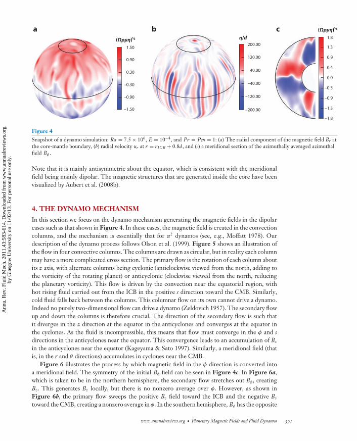
attained, which is fairly independent of Pr = Pm provided Pm ≥ 0.5, but Rm (and so the kineticenergy) is much larger at Pr = Pm = 0.2. Similarly, in Figure 9b the mean B is reasonablyindependent of Pm above 0.5 but is much lower when the inertial regime is reached. To establishthat the transition is indeed connected with inertia, Figure 10 plots the relative strength of theradial components of the Lorentz force |(∇ × B) × B|r , the Coriolis acceleration |2z × u|r , andthe advective part of the inertial acceleration E Pm−1|(∇ × u) × u|r at a randomly chosen time,for points on half of a section parallel to the equatorial plane at z = 0.5d . It is clear that inertiais negligible at the higher Pm values, and Lorentz force is not, whereas at low Pm inertia is largeand Lorentz force is comparatively unimportant in controlling the convection (although it mustplay a role in determining the low magnetic field strength). This inertia-free regime in which themain force balance is between the magnetic Lorentz force (M), the buoyancy, or Archimedeanforce (A), and the Coriolis acceleration (C). This regime is therefore known as the MAC balance,or the magnetostrophic, regime.

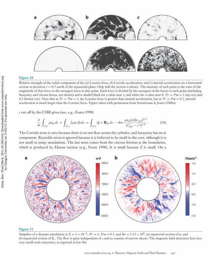
At low E, the dipolar dynamos develop a much finer velocity structure. Figure 11a shows anequatorial section of the radial velocity of a dynamo at E = 3×10−6, Pr = 1, and Pm = 0.1. Thevelocity is only weakly dependent on z, and the fluid motion is more in sheets than in columns.This type of flow has also been found at low E by Kageyama et al. (2008) in a slightly differentmodel. As might be expected given the low Pm, magnetic diffusion is larger than viscous diffusion,and the magnetic field structures shown in Figure 11b are thicker than the velocity structures.This is perhaps the first clear evidence of scale separation between the size of the magnetic andfluid structures.

5.2. J.B. Taylor’s Constraint

J.B. Taylor (1963) showed that if the force balance in the core was magnetostrophic, the magneticfield must satisfy a constraint. The φ component of momentum integrated over a cylinder radius

596 Jones

Ann

u. R

ev. F

luid

Mec

h. 2

011.

43:5

83-6

14. D

ownl

oade

d fr

om w

ww

.ann

ualr

evie

ws.

org

by G

lasg

ow U

nive

rsity

on

11/0

2/13

. For

per

sona

l use

onl

y.


a b c

Figure 10Relative strength of the radial component of the (a) Lorentz force, (b) Coriolis acceleration, and (c) inertial acceleration on a horizontalsection at elevation z = 0.5 north of the equatorial plane. Only half the section is shown. The intensity of each point is the ratio of themagnitude of that force to the strongest force at that point. Each force is divided by the strongest of the forces at each point (includingbuoyancy and viscous forces, not shown) and is shaded black for a value near 1, and white for a value near 0. Pr = Pm = 1 (top row) and0.2 (bottom row). Note that at Pr = Pm = 1, the Lorentz force is greater than inertial acceleration, but at Pr = Pm = 0.2, inertialacceleration is much larger than the Lorentz force. Figure taken with permission from Sreenivasan & Jones (2006a).

s cut off by the CMB gives (see, e.g., Fearn 1998)

∂

∂t

∫C(s )

ρuφ ds +∫

C(s )2ρus � ds =

∫C(s )

( j × B)φ ds − 4π sρuφ(v�rc mb )1/2

(r2c mb − s 2)1/4

. (14)

The Coriolis term is zero because there is no net flow across the cylinder, and buoyancy has no φ

component. Reynolds stress is ignored because it is believed to be small in the core, although it isnot small in many simulations. The last term comes from the viscous friction at the boundaries,which is produced by Ekman suction (e.g., Fearn 1998). It is small because E is small. On a

–500.0

–300.0

–100.0

–1.6

–1.0

–0.3

0.3

1.0

1.6

a b

100.0

300.0

500.0

(Ωρμη)½η/d

Figure 11Snapshot of a dynamo simulation at E = 3 × 10−6, Pr = 1, Pm = 0.1, and Ra = 2.33 × 109: (a) equatorial section of ur and(b) equatorial section of Br . The flow is quite independent of z and so consists of narrow sheets. The magnetic field structures have lessvery-small-scale structures, as expected at low Pm.


Ann

u. R

ev. F

luid

Mec

h. 2

011.

43:5

83-6

14. D

ownl

oade

d fr

om w

ww

.ann

ualr

evie

ws.

org

by G

lasg

ow U

nive

rsity

on

11/0

2/13

. For

per

sona

l use

onl

y.


long-term average, the time-dependent term must be zero, so the Lorentz force balances theEkman suction. Because this is small, but B and j are not, the magnetic field must be constrainedto be in a special configuration that makes the integral almost zero, and this is Taylor’s constraint.Low-E simulations (particularly plane-layer models, which can reach lower E) do seem to satisfyTaylor’s constraint (Rotvig & Jones 2002). The degree to which Taylor’s constraint is satisfied ismonitored by the Taylorization parameter

Tay =∫

C(s ) j × B · 1φd S∫C(s ) |j × B · 1φ | d S

. (15)

Aubert (2005) reported that at low E the Taylorization parameter is becoming small in sphericaldynamos, as did Christensen & Wicht (2007). Takahashi et al. (2005) also claimed to have founda quasi-Taylor state at low E.

Torsional oscillations of the Taylor cylinders about the magnetostrophic equilibrium, torsionalAlfven waves, have been reported in the core with a period of around 50 years (Zatman & Bloxham1997). However, Gillet et al. (2010) have recently found a 6-year oscillation both in the secularvariation of the magnetic field and in the length of the day, which they identify with a torsionaloscillation. If this is correct, it would correspond to an root-mean-square field strength of about4 mT in the core, considerably stronger than the field at the CMB (see Figure 1a). This strongfield is more consistent with current geodynamo models than the much weaker field implied bya 50-year torsional oscillation period. Possible excitation mechanisms are discussed by Dumberry& Bloxham (2003).

5.3. Stress-Free Boundaries

Stress-free boundaries are commonly used on the grounds that the effect of the Ekman boundarylayers that occur in no-slip simulations is overestimated because the Ekman number is too largefor numerical reasons, and it would therefore be better to remove the boundary layers altogether(Kuang & Bloxham 1997). Stress-free nonmagnetic convection simulations lead to much largerzonal flows (axisymmetric flow in the φ direction) than are found with no-slip boundaries, becausethe inertial Reynolds stresses only compete against the internal viscosity and not the much largerboundary layer friction. Consequently, inertial effects, and in particular the effect of zonal flow,are far more apparent in stress-free boundary cases. This leads to a rich dynamical behavior; it ispossible to find quadrupolar dynamos (Simitev & Busse 2005, Busse & Simitev 2006), fluctuatingdynamos (Simitev & Busse 2008), and even hemispherical dynamos, that is, dynamos predomi-nantly in one hemisphere (see Grote & Busse 2000). This work was reviewed in Busse & Simitev(2007). The shear driven by the convection can disrupt the convection, and hence the dynamo.It is therefore possible to obtain regions of reduced shear, where the field and the convection areactive, and regions dominated by shear, where convection is reduced and no field is generated.More recently, it has been noted that in this transition region, multiple steady solutions can befound; that is, with some initial conditions, dipolar dynamos can be found, but with other initialconditions, small-scale dynamos are found at exactly the same parameter values (Simitev & Busse2009). Simply evaluating the strength of the inertial terms in the Earth’s core suggests that theyare very small compared with other terms, except over very short length scales [Sreenivasan &Jones (2006a) estimated length scales below 4 km], which are too small to affect the dynamo.Even small inertial terms can be significant in building zonal flow if they are opposed only bysmall viscous terms in the absence of a magnetic field, but large zonal flows seem unlikely in thepresence of a magnetic field, although Miyagoshi et al. (2010) presented a low-E dynamo with aregion of strong differential rotation outside the field-generating region.

598 Jones

Ann

u. R

ev. F

luid

Mec

h. 2

011.

43:5

83-6

14. D

ownl

oade

d fr

om w

ww

.ann

ualr

evie

ws.

org

by G

lasg

ow U

nive

rsity

on

11/0

2/13

. For

per

sona

l use

onl

y.


5.4. Thermal Boundary Conditions and Internal Heating

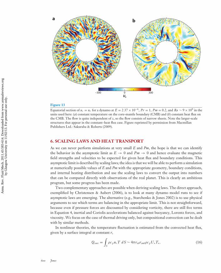
The effect of changing the thermal boundary conditions and adding internal heating was inves-tigated by Kutzner & Christensen (2002). They showed that adding internal heating reduces thedipole dominant region, whereas chemical convection (which acts like thermal convection withan effective heat sink in the outer core) extends the dipolar region (Figure 12). They found thatchanging from a constant-temperature boundary condition to a fixed-flux boundary conditionmade little difference, but Sakuraba & Roberts (2009) looked at low E ∼ 2 × 10−6 (using ourdefinition) and Pm = 1, Pr = 0.2, and found significant differences between fixed-flux andfixed-temperature boundary conditions. In particular, the flow structures are much broader withfixed-flux boundary conditions (see Figure 13), and in consequence flux patches on the CMB aremore significant, as on the Earth. The very fine velocity structures seen in Figures 11a and 13a

lead to a much more dipolar field than the geomagnetic field. Sakuraba & Roberts attribute thedifference to the large-scale flows driven by the temperature differences that appear on the CMBwhen fixed-flux conditions are used.

0 500 1,000 1,500 2,000

1

2

3

4

5

6

7

8

9

Rayleigh number

Model type

Fixed ΔT

Chemical convection

Chemical convection

with fixed-flux ICB

100% internal

heating

50% internal

heating

10% internal

heating

0% internal

heating

Fixed flux at both

boundaries

Fixed T (ICB),

fixed flux (CMB)

N S R

= 0.1Dark blue whole circle area = rms field

Light blue circle area = dipole field = 0.5 = 1.0 failed dynamo

Figure 12Dynamos found with varying boundary conditions and internal heating. E = 3 × 10−4, q = Pm/Pr = 3,and Pr = 1. The Rayleigh number on the scale is a factor E smaller than that defined here. N are regions ofno dynamos, S are stable dipolar dynamos, and R are reversing nondipolar dynamos. The size of the circlesrelates to field strength. Abbreviations: CMB, core-mantle boundary; ICB, inner-core boundary. Figurereprinted from Kutzner & Christensen (2002), with permission from Elsevier.


Ann

u. R

ev. F

luid

Mec

h. 2

011.

43:5

83-6

14. D

ownl

oade

d fr

om w

ww

.ann

ualr

evie

ws.

org

by G

lasg

ow U

nive

rsity

on

11/0

2/13

. For

per

sona

l use

onl

y.


–300 0 300

a b

Us

Figure 13Equatorial section of us = ur for a dynamo at E = 2.37 × 10−6, Pr = 1, Pm = 0.2, and Ra ∼ 9 × 109 in theunits used here: (a) constant temperature on the core-mantle boundary (CMB) and (b) constant heat flux onthe CMB. The flow is quite independent of z, so the flow consists of narrow sheets. Note the larger-scalestructures that appear in the constant–heat flux case. Figure reprinted by permission from MacmillanPublishers Ltd.: Sakuraba & Roberts (2009).

6. SCALING LAWS AND HEAT TRANSPORT

As we can never perform simulations at very small E and Pm, the hope is that we can identifythe behavior in the asymptotic limit as E → 0 and Pm → 0 and hence evaluate the magneticfield strengths and velocities to be expected for given heat flux and boundary conditions. Thisasymptotic limit is described by scaling laws; the idea is that we will be able to perform a simulationat numerically possible values of E and Pm with the appropriate geometry, boundary conditions,and internal heating distribution and use the scaling laws to convert the output into numbersthat can be compared directly with observations of the real planet. This is clearly an ambitiousprogram, but some progress has been made.

Two complementary approaches are possible when deriving scaling laws. The direct approach,exemplified by Christensen & Aubert (2006), is to look at many dynamo model runs to see ifasymptotic laws are emerging. The alternative (e.g., Starchenko & Jones 2002) is to use physicalarguments to see which terms are balancing in the appropriate limit. This is not straightforward,because even if pressure forces are discounted by considering vorticity, there are still five termsin Equation 4, inertial and Coriolis accelerations balanced against buoyancy, Lorentz forces, andviscosity. We focus on the case of thermal driving only, but compositional convection can be dealtwith by similar methods.

In nonlinear theories, the temperature fluctuation is estimated from the convected heat flux,given by a surface integral at constant r,

Qconv =∫

Sρc p ur T d S ∼ 4πricbrcmbρc pU∗T∗, (16)

600 Jones

Ann

u. R

ev. F

luid

Mec

h. 2

011.

43:5

83-6

14. D

ownl

oade

d fr

om w

ww

.ann

ualr

evie

ws.

org

by G

lasg

ow U

nive

rsity

on

11/0

2/13

. For

per

sona

l use

onl

y.


where U∗ and T∗ are the typical velocity and temperature fluctuations, defined in simulations bythe volume integrals over the outer core

U∗ =[

1V

∫u2 dv

]1/2

T∗ =[

1V

∫T 2 dv

]1/2

, (17)

and cp is the specific heat. Recall that T here is the very small superadiabatic temperature, not theactual temperature. The symbol ∼ here means there is a numerical constant of proportionality thatcan be determined by a simulation. The choice 4πricbrcmb follows Christensen & Aubert (2006). Thehope here (and below) is that the same constant will serve for all solutions with the same geometryand boundary conditions. This assumes that there is a strong constant correlation between hotfluid and rising fluid. In rotating convection this is not so clear, but the limited numerical evidencewe possess does give it some support. Note that in a strongly convecting steady state with noheat sources, the total heat flux is independent of r, and so outside of boundary layers, Qconv willalso be independent of r. Astrophysicists use mixing-length theory, a balance between inertia andbuoyancy,

U 2∗ /d ∼ gαT∗ ∼ gαQconv

4πricbrcmbρc pU∗. (18)

In compressible convection, d is usually taken as the density-scale height, and in Boussinesqconvection as the distance between the boundaries. The typical velocity is then the Deardorffvelocity

U∗ ∼(

gαQconvd4πricbrcmbρc p

)1/3

. (19)

The plane-layer version of this works well in laboratory experiments. In the core, for 1 TW ofconvective heat flux, ρ ≈ 104 ms−1, c p ∼ 900 Jkg−1 K−1, g ≈ 8 ms−2, and α ≈ 10−5 K−1, thisgives U∗ about 10 times too big, suggesting that rotation and magnetic field are slowing down theconvection.

6.1. Inertial Theory of Rotating Convection

The essential modification for rotating convection is to allow for tall thin columns, involving thenew short length scale, the column width L⊥. The vorticity (ω) equation, ignoring viscosity, gives

Dω

Dt− 2(� · ∇)u = ∇ × gαT r + 1

ρ∇ × (j × B). (20)

Ignoring (temporarily) the Lorentz force, this suggests that the order-of-magnitude balance is

U 2∗

L2⊥

∼ �U∗d

∼ gαT∗L⊥

, (21)

where the magnitude of the vorticity is U∗/L⊥. The first term comes from nonlinear vorticityadvection over the short length scale L⊥, and the second term comes from the stretching of theplanetary vorticity over the long length scale d due to the motion along the sloping boundaries.Then

L⊥ ∼(

U∗d�

)1/2

∼(

5 × 10−4 × 2 × 106

7 × 10−5

)1/2

∼ 4 km, (22)

where L⊥ is Rhines length, the length scale at which there is a balance of inertial and Corio-lis accelerations. On longer length scales, inertial acceleration is small compared with Coriolisacceleration.


Ann

u. R

ev. F

luid

Mec

h. 2

011.

43:5

83-6

14. D

ownl

oade

d fr

om w

ww

.ann

ualr

evie

ws.

org

by G

lasg

ow U

nive

rsity

on

11/0

2/13

. For

per

sona

l use

onl

y.


As in mixing-length theory, we use Equation 16 to eliminate T∗, and from Equation 21

L⊥ ∼ d(

gαQconv

4πricbrcmb�3d 2ρc p

)1/5

, (23a)

gαT∗ ∼(

�

d

)1/5 (gαQconv

4πricbrcmbρc p

)3/5

, (23b)

U∗�d

= Ro ∼(

gαQconv

4πricbrcmbρc p�3d 2

)2/5

. (24)

Hide (1974) and Ingersoll & Pollard (1982) proposed these scalings, and they were tested ex-perimentally by Aubert et al. (2001). Gillet & Jones (2006) studied them numerically, using thequasi-geostrophic approximation, that is, assuming the vorticity parallel to z is independent of z.For compositional convection, Qconv is replaced by the compositional buoyancy flux. Christensen& Aubert (2006) defined a flux Rayleigh number

RaQ = gαQconv

4πricbrcmbρc p�3d 2. (25)

Fitting data from dynamo simulations, they obtained

Ro = 0.83Ra0.41Q , (26)

which is very close to Equation 24, the inertial scaling. Taking the typical core velocity as 15 kmper year from the secular variation gives Ro = U∗/�d = 2.9 × 10−6, giving

RaQ ∼ 2 × 10−14 → Qconv ∼ 0.6 TW. (27)

This is a reasonable value consistent with independently obtained estimates of the total heat flux.Compositional convection may be releasing a mass flux of 3 × 104 kgs−1 at the ICB, which wouldbe equivalent to RaQ ∼ 8 × 10−13. This would give a rather high value for the typical velocity inthe core, 60 km per year.

One problem with Equations 23 and 24 is that they predict that L⊥ has a very small value ofabout 4 km in the core. If we assume that the magnetic field prevents L⊥ from becoming this small,a fixed value of L⊥ rather than that given in Equation 23a leads to an exponent of 1/2 rather than2/5 in Equation 24, as suggested by Starchenko & Jones (2002). This would give a slightly lowervelocity for the given compositional mass flux.

6.2. Magnetic Field Strength

In the Earth’s core, magnetic energy is much greater than kinetic energy, so a simple equipar-tition as used in astrophysics will not work here. One approach (Christensen & Aubert 2006)to estimating the field strength is through estimating the rate of ohmic dissipation. The rate ofworking of the buoyancy force equals the rate of ohmic and viscous dissipation in a steady state.We denote the fraction of ohmic dissipation to the total dissipation as fohm. In dynamo models therate of ohmic dissipation is typically similar to the rate of viscous dissipation, fohm ≈ 0.5, but thelow Pm suggests a value closer to unity might be more appropriate in the core. We can estimatethe buoyancy force work in terms of the heat flux by taking the scalar product of Equation 4 withu and integrating over the whole outer core, so∫

ημj2 dv = fohm

∫gα

c p

[∫ρc p ur T ′ d S

]dr ≈ 7.01 fohmρ�3d 5 RaQ (28)

for the geometry of the Earth’s core (Christensen & Aubert 2006).

602 Jones

Ann

u. R

ev. F

luid

Mec

h. 2

011.

43:5

83-6

14. D

ownl

oade

d fr

om w

ww

.ann

ualr

evie

ws.

org

by G

lasg

ow U

nive

rsity

on

11/0

2/13

. For

per

sona

l use

onl

y.


Now we need to relate the magnetic energy to ohmic dissipation. The dissipation time isthe time taken for the magnetic energy to be dissipated through ohmic loss, which for a solidconductor would scale as d 2/η. For a whole sphere of radius a, Moffatt (1978) gave the e-foldingtime as τdiss = a2/π2η. Christensen & Tilgner (2004) proposed that in a turbulent fluid, thistime would be reduced by a factor Rm, the magnetic Reynolds number, so then τdiss ∼ d/U∗,independent of η. Equivalently, we can think of the dissipation taking place over a short lengthscale d Rm−1/2, which is the expected length scale if the magnetic field is concentrated into fluxropes (Galloway et al. 1977), which then dominate the dissipation. Then∫

ημj2 dv ∼ Rmη

d 2

∫B2/2μ dv. (29)

We now have ∫ημj2 dv ∼ U∗

d

∫B2

μdv ∼ fohmρ�3d 5 RaQ. (30)

Using Equation 24 to estimate U∗, this gives

B∗ ∼ (μ fohmρ)1/2�d (RaQ)3/10 ∼ (μ fohm)1/2d−1/5ρ1/5�1/10(

gαQconv

c p

)0.3

. (31)

The remarkable feature is the weak dependence of B∗ on �. We are assuming, however, that theplanet is in the rapidly rotating low Ro regime for these estimates to be plausible. This estimatedoes give sensible field strengths for the Earth and Jupiter (Christensen & Aubert 2006), the twoplanets for which we have reasonable estimates for the heat flux and the other physical quantitiesin the formula.

It is not easy to reconcile Equation 31 with the balance in the vorticity equation given inEquation 20, which is slightly worrying as the fundamental MAC balance in the core is believed tobe between the buoyancy force, Lorentz force, and Coriolis acceleration. The simplest estimatefor the Lorentz force in Equation 20 is B2

∗/μL2⊥, and balancing this against the Coriolis estimate

ρ�U∗/d gives

B∗ ∼ (μρ)1/2�d Ra2/5Q , (32)

slightly different from Equation 31 and significantly smaller in the core. A more detailed modelwould be to balance the buoyant driving and vortex stretching in the z-vorticity equation withthe magnetic friction torque from the Bφ component of the magnetic field. One might reasonablyassume that the length scale L⊥ is set by the balance of induction and diffusion in the inductionequation, leading to B∗U∗ ∼ ημj∗, which in the vorticity equation gives

B∗ ∼ (�ρμη)1/2(

L⊥d

)1/2

. (33)

In the range of simulations, none of the three estimates given in Equations 31–33 is very different,and each depends on how L⊥ scales at low RaQ, which is unclear because, as mentioned above, itseems unlikely that Equation 23a continues to be valid in the asymptotic limit. It is also worthnoting that Equation 31 estimates B∗ from the total magnetic energy rather than the average of themodulus of the field. At large Rm there may be concentrated flux ropes at which the field is locallymuch larger than its typical value. The magnetic energy B2/μ is then dominated by these fluxropes, and the estimate given in Equation 31 would be significantly larger than the typical valueoutside the ropes. The estimate given in Equation 33, alternatively, might relate to the lowestvalues of the Bφ field, where the magnetic damping of the convective rolls is weaker. It is clearthat more work needs to be done before we can be confident about the correct scaling laws, butnevertheless an encouraging start has been made.


Ann

u. R

ev. F

luid

Mec

h. 2

011.

43:5

83-6

14. D

ownl

oade

d fr

om w

ww

.ann

ualr

evie

ws.

org

by G

lasg

ow U

nive

rsity

on

11/0

2/13

. For

per

sona

l use

onl

y.


7. MODELS OF THE MAGNETIC FIELDS OF INDIVIDUAL PLANETS

7.1. Mercury

Mercury has a radius of only 2,440 km, but it has a relatively large fluid core, with a radius of about1,900 km. Space missions have enabled the dipole moment, 4.2 × 1012 Tm3, and the low-orderGauss coefficients to be determined (Uno et al. 2009), and the radial component of the field at theCMB is shown in Figure 14. The field pattern is not too dissimilar from the geomagnetic fieldtruncated at degree 3, but the field strength is about 500 times weaker than the Earth’s CMB field.This difference has been considered to result from Mercury’s slow rotation period, 59 days, but themore recent view is that field strength is only weakly dependent on rotation, provided the Rossbynumber is small. Two dynamo models accounting for Mercury’s weak field have been proposed.Christensen (2006) suggested that only the deepest part of Mercury’s outer core is convecting;the upper parts may be stably stratified [as has been proposed for the Earth by Willis et al. (2007),although Mercury’s stable layer is assumed much deeper]. The dynamo in the lower core is thenoperating in essentially the same way as the geodynamo, but the stable conducting regions onlyallow a small fraction of the field to escape to the surface, and they filter out all the high-degreeharmonics. Hence the observed field of Mercury appears much weaker. An alternative thin-shellmodel was proposed by Stanley et al. (2005). Compositional convection may be more advancedin Mercury, leaving only a thin shell of liquid with a high concentration of light material, therest being solid iron. A thin-shell dynamo would have more power in the higher harmonics, notobservable (so far) from space missions, and a relatively weak dipolar component. Also they arguethat the ω-effect could be more important in thin-shell dynamos, with the field being limited bya large unobservable toroidal component. As these two theories make quite different predictionsfor the magnetic spectrum, the new missions to Mercury might help decide between them.

7.2. Earth

There is a large literature on models of the Earth’s magnetic field, a good source being volume 5of the Treatise of Geophysics edited by Kono (2007). Here we briefly overview a selection of topicsthat have attracted attention recently.

–1,600 nT 1,600 nT


Figure 14The radial component of Mercury’s magnetic field at its core-mantle boundary, centered on longitude zero.

604 Jones

Ann

u. R

ev. F

luid

Mec

h. 2

011.

43:5

83-6

14. D

ownl

oade

d fr

om w

ww

.ann

ualr

evie

ws.

org

by G

lasg

ow U

nive

rsity

on

11/0

2/13

. For

per

sona

l use

onl

y.


7.2.1. Polar vortices. Dynamo models often show a significant difference between the polarregions inside the tangent cylinder and the rest of the outer core, a consequence of the columnarstructure of the convection. Olson & Aurnou (1999) found geomagnetic evidence that the polarregions have an anticyclonic vortex. They suggested this might be due to excess heat and lightmaterial released from the ICB. From the thermal wind equation, the φ component of the vorticityequation,

2�∂uφ

∂z= gα

r∂T∂θ

, (34)

the resulting latitudinal temperature gradient (or composition gradient) makes the flow anticy-clonic near the CMB and cyclonic near the ICB. Glatzmaier & Roberts (1996a) proposed that thismight mean that the inner core is rotating slightly faster than the mantle, for which there has beensome seismological evidence. More recently, this inner-core super-rotation has been questioned,and Buffett & Glatzmaier (2000) suggested that gravitational coupling between a slightly nonax-isymmetric inner core and mantle might in fact lock the rotation of the inner core to the mantle.Aurnou et al. (2003) showed that polar vortices of the correct sign of vorticity could be produced inlaboratory convection with a hemispherical inner core. Sreenivasan & Jones (2005, 2006b) foundpolar vortices in dynamo simulations but noted that the Lorentz force played a significant role inthe thermal wind equation.

7.2.2. History of the geodynamo and reversals. Models of the thermal history of the Earthsuggest that the inner core only started forming about 1 Gyr ago (Labrosse et al. 2001), muchless than the age of the Earth, 4.5 Gyr. Because the inner core generates most of the heat fluxand all the mass flux in the standard model, Roberts et al. (2003) suggested that there must beradioactivity in the core to provide the heat flux necessary to drive the dynamo prior to inner-coreformation. Paleomagnetic evidence suggests that the dynamo has been working at more or lessits present strength for at least 3.5 Gyr. Aubert et al. (2009) have examined the secular changes indynamo activity as heat and composition sources evolve.

Glatzmaier & Roberts (1995) found a dynamo that had quite earthlike reversals. Sarson &Jones (1999) analyzed a reversing dynamo and suggested that the origin of the reversals lay influid breaking out of the thermal boundary layer near the ICB, giving rise to buoyancy surges.Large Ra was necessary for this to occur, which is numerically difficult. Kutzner & Christensen(2004) explored earthlike reversals near the transition between the inertia and inertia-free regimes,an idea developed by Olson & Christensen (2006), who gave criteria for a dynamo to be in thisreversing regime.

7.2.3. Mantle heterogeneity. The heat flux taken out of the core by the mantle is likely to varystrongly with position, being highest where cool descending slabs from subducting plates reachthe CMB. This heterogeneity can be estimated using seismic tomography (see, e.g., Gubbinset al. 2007) and will couple dynamo activity in the core to long geological timescales. Glatzmaieret al. (1999) found that reversals in dynamo models were strongly affected by the distribution ofheat flux over the CMB, with some arrangements preventing reversals and others encouragingthem. They proposed that the long Cretaceous superchron, 40 Myr during which there wereno reversals, resulted from mantle convection giving rise to a CMB heat flux distribution thatsuppressed reversals. Heterogeneous CMB heat flux has also been proposed as an explanationfor the preferred reversal paths noted by Hoffman (1992) and the persistent flux patches overCanada and Siberia (Gubbins & Kelly 1993). The effects of heterogeneous CMB heat flux ondynamo models have been investigated by Willis et al. (2007). Mantle inhomogeneity might affect


Ann

u. R

ev. F

luid

Mec

h. 2

011.

43:5

83-6

14. D

ownl

oade

d fr

om w

ww

.ann

ualr

evie

ws.

org

by G

lasg

ow U

nive

rsity

on

11/0

2/13

. For

per

sona

l use

onl

y.


convection throughout the outer core, and hence lead to inhomogeneity in the way freezing takesplace at the ICB (Aubert et al. 2008a).

7.3. Mars

The Mars Global Surveyor discovered strong remanent magnetism on Mars (Acuna et al. 2001),suggesting that it had an ancient dynamo. The age at which it stopped working, around 350 Myrafter the formation of the planet, can be estimated by studying the geology of Mars (Lillis et al.2008). It is known that Mars still has a liquid core (Yoder et al. 2003), so the simplest explanationis that the core stopped convecting and hence the power source failed. Kuang et al. (2008) used adynamo model to show that a dynamo can collapse quite suddenly, due to its subcritical nature.The martian magnetic field is predominantly in one hemisphere, which led Stanley et al. (2008)to propose a model based on an asymmetric convection pattern, which might have been inducedby the crustal asymmetry of that planet, the northern hemisphere crust being significantly thinnerthan that of the southern hemisphere uplands.

7.4. Ganymede

Ganymede’s magnetic field was discovered by the Galileo spacecraft (Kivelson et al. 1996). Thefirst problem was whether this was a genuine dynamo or merely an amplifier of Jupiter’s magneticfield. Models by Sarson et al. (1997) concluded that a dynamo was more likely. Ganymede hasan icy crust, a warm silicate mantle, and a metallic core. The radius is 2,634 km, but the metalliccore radius is believed to be (from gravity measurements) approximately 500 km. The dipolemoment is 1.3 × 1013 Tm3, about three times larger than that of Mercury. At the surface the fieldis typically 700 nT, but at the CMB this rises to 0.12 mT, weaker than the Earth’s CMB fieldbut much stronger than Mercury’s field. The outstanding problem with the Ganymede dynamois the energy source. It is surprising that such a small body is still convecting; Showman et al.(1997) suggested that orbital resonances might lead to tidal heating, but this is still controversial(Bland et al. 2008). If Ganymede does indeed have a dynamo, it raises the interesting question ofhow small a planetary body can be and still have a dynamo. The recent discovery of microteslamagnetic fields on angrites (Weiss et al. 2008), meteorites that record the earliest history of thesolar system, suggests that planetesimal components that subsequently formed the planets mighthave had their own dynamos.

7.5. The Giant Planets

All the outer planets are believed to be transporting heat by convection, so fluid motion is expectedin their interiors. The very high pressures found in Jupiter and Saturn lead to metallic hydrogen;that is, the gas becomes ionized and hence electrically conducting. This electrical conductivityrises gradually with depth, reaching a plateau of 2 × 105 Sm−1 (Nellis 2000), three times lowerthan the usual estimate for the Earth’s metallic core, 6×105 Sm−1 (see, e.g., Merrill et al. 1996). InJupiter, the plateau is reached at a radius about 0.8 RJ, whereas in smaller Saturn, where the highpressures needed are found only deeper, it is reached at about 0.5 RS. The Gauss coefficients forJupiter and Saturn up to degree 3 are reconstructed from space-mission results, and are listed inConnerney (1993). There is some doubt as to where the dynamo is actually operating in the giantplanets, because the overall magnetic Reynolds number is large, and it may be that dynamo actionworks best at moderate Rm. If this is true, regions where the electrical conductivity is below itsmaximum value may be optimal, in which case the magnetic region could extend above 0.8 RJ and

606 Jones

Ann

u. R

ev. F

luid

Mec

h. 2

011.

43:5

83-6

14. D

ownl

oade

d fr

om w

ww

.ann

ualr

evie

ws.

org

by G

lasg

ow U

nive

rsity

on

11/0

2/13

. For

per

sona

l use

onl

y.


–1.2 mT 1.2 mT

–0.06 mT 0.06 mT

a

b



Figure 15The radial component of (a) Jupiter’s magnetic field and (b) Saturn’s magnetic field, both at the surface usingthe Hammer-Aitoff projection, centered on longitude −180◦ west.

0.5 RS. Figures 15a,b show the magnetic fields of Jupiter and Saturn at their surface. Jupiter’s field(based on the Gauss coefficients given in Connerney 1993) is essentially a dipolar field inclined atabout 10◦ to the rotation axis, similar to the Earth. Jupiter’s rotation rate is defined by the rotationperiod of its magnetic field, which is accurately known. The surface features rotate at different ratesdepending on their latitude. This observation alone suggests that the typical convective velocityin the deep interior must be much less than the fast east-west jet flows at the surface, which canreach over 100 ms−1 in Jupiter and 300 ms−1 in Saturn. Observations of changes in the magneticfield of Jupiter between the Voyager and Galileo missions suggest flows on the order of 10−3 ms−1

are moving the field around (Russell et al. 2001).As is clear from Figure 15b, Saturn’s magnetic field (based on the Gauss coefficients given

in Burton et al. 2009) is remarkably axisymmetric, so much so that its rotation period cannotbe reliably determined from its magnetic field, so the rotation rate of Saturn’s deep interioris still uncertain. Saturn’s field is also significantly weaker than Jupiter’s field, but it should beremembered that the metallic hydrogen region in Saturn is at a depth of half its radius, so thefield at its effective CMB could be nearly 10 times larger. Cowling’s (1934) theorem tells us thataxisymmetric fields cannot be generated by dynamo action, so assuming the dynamo hypothesis


Ann

u. R

ev. F

luid

Mec

h. 2

011.

43:5

83-6

14. D

ownl

oade

d fr

om w

ww

.ann

ualr

evie

ws.

org

by G

lasg

ow U

nive

rsity

on

11/0

2/13

. For

per

sona

l use

onl

y.


is correct, the generated field must be nonaxisymmetric, but processes outside the main dynamoregion must be making the observed part of the field axisymmetric. Stevenson (1982) suggestedthat differential rotation in a stably stratified region outside the dynamo-generating core might beresponsible, an idea supported by numerical simulations including a stably stratified outer layer(Christensen & Wicht 2008).

7.6. The Ice Giants

Uranus and Neptune both have rather irregular nondipolar fields, as illustrated in Figure 16. Thiswas a quite surprising discovery as all previously known planetary fields were essentially dipolar.Indeed, it is quite surprising that these ice giants have a magnetic field at all, as they are too smallto form metallic hydrogen and have no liquid-iron core. It is believed that ionic conductivity inthe fluid ionic layer between 0.3 Rs and 0.8 Rs allows sufficient electric currents to flow (Cavazzoniet al. 1999). However, the predicted electrical conductivity is only 3 × 103 S m−1, which does leadto an uncomfortably small magnetic Reynolds number unless the fluid velocities in the dynamo

a

b

–0.12 mT 0.12 mT

–0.1 mT 0.1 mT



Figure 16The radial component of (a) Uranus’s magnetic field and (b) Neptune’s magnetic field, both at the surfaceusing the Hammer-Aitoff projection, centered on longitude −180◦ west. Data taken from Holme &Bloxham (1996).

608 Jones

Ann

u. R

ev. F

luid

Mec

h. 2

011.

43:5

83-6

14. D

ownl

oade

d fr

om w

ww

.ann

ualr

evie

ws.

org

by G

lasg

ow U

nive

rsity

on

11/0

2/13

. For

per

sona

l use

onl

y.


region are significantly larger than those in other planetary cores. The difficulty is compoundedin the case of Uranus by the small heat flux emerging from the planet, which if taken at face valuewould suggest a smaller convective velocity rather than a larger one. A further problem is thatthe ohmic dissipation in these ice giants turns out to be quite large (Holme & Bloxham 1996).Nevertheless, a dynamo model has been constructed (Stanley & Bloxham 2006). Their model hasa stably stratified layer below the main dynamo region, which might also account for the low heatflux. This region allows the generated field to move around more than in models with a solid innercore, and this gives rise to nondipolar fields.

8. PERSPECTIVES AND FUTURE DEVELOPMENTS

Dynamo models have developed rapidly over the past 10 years, and the early successes in simulatingthe geodynamo have developed into quite detailed models of the magnetic fields of other planets.There is now a much greater coverage of the parameter space in the models, and the effects ofvarying driving, boundary conditions and parameter values are beginning to be understood. Itis clear that a great diversity of behavior can arise in the models, but this is consistent with thediversity of planetary magnetic fields themselves. Another encouraging development is that thephysical mechanisms behind dynamo action in the simulations are becoming better understood.Until recently, the numerical codes were essentially black boxes giving rather unpredictable resultsfor each new parameter set. This encouraged researchers to adjust parameters, often motivatedby numerical rather than physical reasons, until they found the behavior they wanted. This eradoes seem to be coming to an end, with the simulations now being used as a tool to explore newphysical ideas relevant to planetary cores.

For the geodynamo, observations have given us a data set of the geomagnetic field over the past300 years, with high-accuracy values over the past 30 years. Work is currently in progress to tryto assimilate this data into geodynamo models (Gillet et al. 2009). The immediate aim here is touse this data to discriminate between different dynamo models. The dynamo model is thus a givenprior, to which noisy observational data are added, the output being a time-dependent model ofthe geomagnetic field. A poor dynamo model leads to large residuals, a better model to smallerresiduals. Ultimately, it may be possible to use these techniques to forecast the geomagnetic field(Kuang et al. 2009), but it is in the nature of the geodynamo equations (as it is with weatherforecasting) that predictions far into the future will not be possible (Hulot et al. 2010).

We cannot, and probably never will be able to, use the true very low values of the dissipationin simulations. This problem is being overcome by understanding how the models behave in theasymptotic limit, the scaling-law approach, and although much remains to be done, the path aheadseems clear. However, the models that emerge as new computational resources allow us to moveinto the low-E, low-inertia, regime are if anything becoming less earthlike than the moderateE ∼ 10−4 solutions, which were the lowest that could be reached 10 years ago. In particular,recent low-E models are often very dipole dominant and show no prospect of reversing. It is toosoon to say that there must be something fundamentally wrong with our overall physical picture;it is possible that higher Rayleigh numbers, better boundary conditions, improved modeling,and possibly compressible effects will give more earthlike behavior. It is also true that numericalconstraints can be quite insidious, in that they force us into particular parameter regimes, leadingto a false impression of the overall behavior. However, our improving understanding of dynamoprocesses and spherical convection may well make it possible to develop physically based earthlikemodels in the near future.

The general outlook for the subject remains extremely promising. New models of giant planetdynamos are ripe for progress, and the development of compressible planetary dynamo models


Ann

u. R

ev. F

luid

Mec

h. 2

011.

43:5

83-6

14. D

ownl

oade

d fr

om w

ww

.ann

ualr

evie

ws.

org

by G

lasg

ow U

nive

rsity

on

11/0

2/13

. For

per

sona

l use

onl

y.


is a major area for future research. There is a real possibility of discovering magnetic fields onexoplanets, which would give a huge new impetus to the subject. Analysis of magnetic fields in theremnants of the forming solar system may also help us to understand the origin of our planets.

DISCLOSURE STATEMENT

The author is not aware of any affiliations, memberships, funding, or financial holdings that mightbe perceived as affecting the objectivity of this review.

ACKNOWLEDGMENTS

I would like to thank Binod Sreenivasan, David Gubbins, and Phil Livermore for many usefuldiscussions, which helped the preparation of this article. I am also grateful to Richard Holme, UliChristensen, and Ataru Sakuraba for providing original figures. Thanks are due to the LeverhulmeTrust, for providing support through grant F/00122/AD.

LITERATURE CITED

Acuna MH, Connerney JE, Ness NF, Lin RP, Mitchell D, et al. 1999. Global distribution of crustal magne-tization discovered by the Mars Global Surveyor MAG/ER experiment. Science 284:790–93

Anufriev AP, Jones CA, Soward AM. 2005. The Boussinesq and anelastic liquid approximations for convectionin the Earth’s core. Phys. Earth Planet. Inter. 152:163–90

Aubert J. 2005. Steady zonal flows in spherical shell dynamos. J. Fluid Mech. 542:53–67Aubert J, Amit H, Hulot G, Olson P. 2008a. Thermochemical flows couple the Earth’s inner core growth to

mantle heterogeneity. Nature 454:758–61Aubert J, Aurnou J, Wicht J. 2008b. The magnetic structure of convection-driven numerical dynamos.

Geophys. J. Int. 172:945–56Aubert J, Brito D, Nataf H-C, Cardin P, Masson J-P. 2001. A systematic experimental study of rapidly rotating

spherical convection in water and liquid gallium. Phys. Earth Planet. Inter. 128:51–74Aubert J, Labrosse S, Poitou C. 2009. Modelling the palaeo-evolution of the geodynamo. Geophys. J. Int.

179:1414–28Aurnou J, Andreadis S, Zhu L, Olson P. 2003. Experiments on convection in Earth’s core tangent cylinder.

Earth Planet. Sci. Lett. 212:119–34Bland MT, Showman AP, Tobie G. 2008. The production of Ganymede’s magnetic field. Icarus 198:384–99Braginsky SI, Meytlis VP. 1990. Local turbulence in the Earth’s core. Geophys. Astrophys. Fluid Dyn. 55:71–87Braginsky SI, Roberts PH. 1995. Equations governing convection in Earth’s core and the geodynamo. Geophys.

Astrophys. Fluid Dyn. 79:1–97Buffett BA, Glatzmaier GA. 2000. Gravitational braking of inner-core rotation in geodynamo simulations.

Geophys. Res. Lett. 27:3125–28Bullard EC. 1949. The magnetic field within the Earth. Proc. R. Soc. Lond. A 197:433–53Burton ME, Dougherty MK, Russell CT. 2009. Model of Saturn’s internal planetary magnetic field based on

Cassini observations. Planet. Space Sci. 57:1706–13Busse FH. 1970. Thermal instabilities in rapidly rotating systems. J. Fluid Mech. 44:441–60Busse FH. 2000. Homogeneous dynamos in planetary cores and in the laboratory. Annu. Rev. Fluid Mech.

32:383–408Busse FH, Simitev RD. 2006. Parameter dependences of convection-driven dynamos in rotating spherical

fluid shells. Geophys. Astrophys. Fluid Dyn. 100:341–61Busse FH, Simitev RD. 2007. Planetary dynamos. In Treatise on Geophysics, Vol. 10, ed. T Spohn, pp. 281–98.

Amsterdam: ElsevierCavazzoni C, Chiarotti GL, Scandolo S, Tosatti E, Bernasconi M, Parrinello M. 1999. Superionic and metallic

states of water and ammonia at giant planet conditions. Science 283:44–46

610 Jones

Ann

u. R

ev. F

luid

Mec

h. 2

011.

43:5

83-6

14. D

ownl

oade

d fr

om w

ww

.ann

ualr

evie

ws.

org

by G

lasg

ow U

nive

rsity

on

11/0

2/13

. For

per

sona

l use

onl

y.


Christensen UR. 2006. A deep dynamo generating Mercury’s magnetic field. Nature 444:1056–58Christensen UR, Aubert J. 2006. Scaling properties of convection-driven dynamos in rotating spherical shells

and application to planetary magnetic fields. Geophys. J. Int. 166:97–114Christensen UR, Aubert J, Cardin P, Dormy E, Gibbons S, et al. 2001. A numerical dynamo benchmark. Phys.

Earth Planet. Inter. 128:25–34Christensen UR, Olson P, Glatzmaier GA. 1999. Numerical modeling of the geodynamo: a systematic

parameter study. Geophys. J. Int. 138:393–409Christensen UR, Tilgner A. 2004. Power requirement of the geodynamo from ohmic losses in numerical and

laboratory dynamos. Nature 429:169–71Christensen UR, Wicht J. 2007. Numerical dynamo simulations. See Olson 2007, pp. 245–82Christensen UR, Wicht J. 2008. Models of magnetic field generation in partly stable planetary cores: applica-

tions to Mercury and Saturn. Icarus 196:16–34Clune TC, Elliot JR, Miesch MS, Toomre J, Glatzmaier GA. 1999. Computational aspects of a code to study

rotating turbulent convection in spherical shells. Parallel Comput. 25:361–80Connerney JEP. 1993. Magnetic fields of the outer planets. J. Geophys. Res. Planets 98:18659–79Cowling TG. 1934. The magnetic field of sunspots. MNRAS 94:39–48Dormy E, Soward AM, Jones CA, Jault D, Cardin P. 2004. The onset of thermal convection in rotating

spherical shells. J. Fluid Mech. 501:43–70Dumberry M, Bloxham J. 2003. Torque balance, Taylor’s constraint and torsional oscillations in a numerical

model of the geodynamo. Phys. Earth Planet. Inter. 140:29–51Elsasser WM. 1939. On the origin of the Earth’s magnetic field. Phys. Rev. 55:489–98Fearn D. 1998. Hydromagnetic flow in planetary cores. Rep. Prog. Phys. 61:175–235Galloway DJ, Proctor MRE, Weiss NO. 1977. Formation of intense magnetic fields near the surface of the

Sun. Nature 266:686–89Gillet N, Jones CA. 2006. The quasi-geostrophic model for rapidly rotating spherical convection outside the

tangent cylinder. J. Fluid Mech. 554:343–69Gillet N, Jault D, Canet E, Fournier A. 2010. Fast torsional waves and strong magnetic field within the Earth’s

core. Nature 465:74–77Gillet N, Pais MA, Jault D. 2009. Ensemble inversion of time-dependent core flow models. Geochem. Geophys.

Geosyst. 10:Q06004Glatzmaier GA, Coe RS. 2007. Magnetic polarity reversals in the core. See Olson 2007, pp. 283–97Glatzmaier GA, Coe RS, Hongre L, Roberts PH. 1999. The role of the Earth’s mantle in controlling the

frequency of geomagnetic reversals. Nature 401:885–90Glatzmaier GA, Roberts PH. 1995. A three-dimensional self-consistent computer simulation of a geomagnetic

field reversal. Nature 377:203–9Glatzmaier GA, Roberts PH. 1996a. Rotation and magnetism of the Earth’s inner core. Science 274:1887–91Glatzmaier GA, Roberts PH. 1996b. An anelastic evolutionary geodynamo simulation driven by compositional

and thermal convection. Physica D 97:81–94Glatzmaier GA, Roberts PH. 1997. Simulating the geodynamo. Contemp. Phys. 38:269–88Grote E, Busse FH. 2000. Hemispherical dynamos generated by convection in rotating spherical shells. Phys.

Rev. E 62:4457–60Gubbins D, Jones AL, Finlay CC. 2006. Fall in Earth’s magnetic field is erratic. Science 312:900–2Gubbins D, Kelly P. 1993. Persistent patterns in the geomagnetic field during the last 2.5 Myr. Nature

365:829–32Gubbins D, Willis AP, Sreenivasan B. 2007. Correlation of Earth’s magnetic field with lower mantle thermal

and seismic structure. Phys. Earth Planet. Inter. 162:256–60Hide R. 1974. Jupiter and Saturn. Proc. R. Soc. Lond. A 336:63–84Hoffman KA. 1992. Dipolar reversal states of the geomagnetic field and core mantle dynamics. Nature 359:789–

94Holme R. 2007. Large-scale flow in the core. See Olson 2007, pp. 107–30Holme R, Bloxham J. 1996. The magnetic fields of Uranus and Neptune: methods and models. J. Geophys.

Res. Planets 101:2177–200


Ann

u. R

ev. F

luid

Mec

h. 2

011.

43:5

83-6

14. D

ownl

oade

d fr

om w

ww

.ann

ualr

evie

ws.

org

by G

lasg

ow U

nive

rsity

on

11/0

2/13

. For

per

sona

l use

onl

y.


Holme R, Olsen N. 2006. Core surface flow modelling from high-resolution secular variation. Geophys. J. Int.166:518–28

Hughes DW. 2007. Nonlinear effects in mean field dynamo theory. In Mathematical Aspects of Natural Dynamos,ed. E Dormy, AM Soward, pp. 79–97. Boca Raton, FL: CRC

Hulot G, Lhuillier F, Aubert J. 2010. Earth’s dynamo limit of predictability. Geophys. Res. Lett. 37:L06305Ingersoll AP, Pollard D. 1982. Motions in the interiors and atmospheres of Jupiter and Saturn: scale analysis,

anelastic equations, barotropic stability criterion. Icarus 52:62–80Jackson A. 2003. Intense equatorial flux spots on the surface of the Earth’s core. Nature 424:760–63Jackson A, Livermore P. 2009. On Ohmic heating in the Earth’s core I: nutation constraints. Geophys. J. Int.

177:367–82Jones CA. 2000. Convection driven geodynamo models. Philos. Trans. R. Soc. Lond. A 358:873–97Jones CA. 2003. Dynamos in planets. In Stellar Astrophysical Fluid Dynamics, ed. MJ Thompson, J Christensen-

Dalsgaard, pp. 159–76. Cambridge, UK: Cambridge Univ. PressJones CA. 2007a. Planetary dynamos. In Mathematical Aspects of Natural Dynamos, ed. E Dormy, AM Soward,

pp. 257–80. Boca Raton, FL: CRCJones CA. 2007b. Thermal and compositional convection in the outer core. See Olson 2007, pp. 131–85Jones CA, Kuzanyan KM. 2009. Compressible convection in the deep atmospheres of giant planets. Icarus

204:227–38Jones CA, Kuzanyan KM, Mitchell RH. 2009. Linear theory of compressible convection in rapidly rotating

spherical shells, using the anelastic approximation. J. Fluid Mech. 634:291–319Jones CA, Longbottom AW, Hollerbach R. 1995. A self-consistent convection driven geodynamo model,

using a mean field approximation. Phys. Earth Planet. Inter. 92:119–41Jones CA, Soward AM, Mussa AI. 2000. The onset of convection in a rapidly rotating sphere. J. Fluid Mech.

405:157–79Kageyama A, Miyagoshi T, Sato T. 2008. Formation of current coils in geodynamo simulations. Nature

454:1106–9Kageyama A, Sato T. 1997. Velocity and magnetic field structures in a magnetohydrodynamic dynamo. Phys.

Plasmas 4:1569–75Kageyama A, Sato T, Watanabe K, Horiuchi R, Hayashi T, et al. 1995. Computer simulation of a magneto-

hydrodynamic dynamo. II. Phys. Plasmas 2:1421–31Kivelson MG, Khurana KK, Russell CT, Walker RJ, Warnecke J, et al. 1996. Discovery of Ganymede’s

magnetic field by the Galileo spacecraft. Nature 384:537–41Kono M, Roberts PH. 2002. Recent geodynamo simulations and observations of the geomagnetic field. Rev.

Geophys. 40:1013Kono M, ed. 2007. Treatise on Geophysics, Vol. 5. Amsterdam: ElsevierKuang W, Bloxham J. 1997. An Earth-like numerical dynamo model. Nature 389:371–74Kuang W, Jiang W, Wang T. 2008. Sudden termination of Martian dynamo? Implications from subcritical

dynamo simulations. Geophys. Res. Lett. 35:L14204Kuang WJ, Tangborn A, Wei ZG, Sabaka T. 2009. Constraining a numerical geodynamo model with 100 years

of surface observations. Geophys. J. Int. 179:1458–68Kutzner C, Christensen UR. 2002. From stable dipolar towards reversing numerical dynamos. Phys. Earth

Planet. Inter. 131:29–45Kutzner C, Christensen UR. 2004. Simulated geomagnetic reversals and preferred virtual geomagnetic pole

paths. Geophys. J. Int. 157:1105–18Labrosse S, Poirier JP, LeMouel JL. 2001. The age of the inner core. Earth Planet. Sci. Lett. 190:111–23Larmor J. 1919. How could a rotating body such as the Sun become a magnet? Rep. Br. Assoc. Adv. Sci.

87:159–60Lillis RJ, Frey HV, Manga M, Mitchell DL, Lin RP, et al. 2008. An improved crustal magnetic map of Mars

from electron reflectometry: highland volcano magmatic history and the end of the martian dynamo.Icarus 194:575–96

Malkus WVR. 1994. Energy sources for planetary dynamos. In Lectures on Solar and Planetary Dynamos, ed.MRE Proctor, AD Gilbert, pp. 161–79. Cambridge, UK: Cambridge Univ. Press

612 Jones

Ann

u. R

ev. F

luid

Mec

h. 2

011.

43:5

83-6

14. D

ownl

oade

d fr

om w

ww

.ann

ualr

evie

ws.

org

by G

lasg

ow U

nive

rsity

on

11/0

2/13

. For

per

sona

l use

onl

y.


Maus S, Macmillan S, Lowes F, Bondar T. 2005. Evaluation of candidate geomagnetic field models for the10th generation of IGRF. Earth Planets Space 57:1173–81

Merrill RT, McElhinny MW, McFadden PL. 1996. The Magnetic Field of the Earth. Vol. 63 Int. Geophys. Ser.New York: Academic

Miyagoshi T, Kageyama A, Sato T. 2010. Zonal flow formation in the Earth’s core. Nature 463:793–97Moffatt HK. 1978. Magnetic Field Generation in Electrically Conducting Fluids. Cambridge, UK: Cambridge

Univ. Press. 343 pp.Nellis WJ. 2000. Metallization of fluid hydrogen at 140 GPa (1.4 Mbar): implications for Jupiter. Planet. Space

Sci. 48:671–77Olson P, ed. 2007. Treatise on Geophysics, Vol. 8. Amsterdam: ElsevierOlson P, Aurnou J. 1999. A polar vortex in the Earth’s core. Nature 402:170–73Olson P, Christensen UR. 2006. Dipole moment scaling for convection-driven planetary dynamos. Earth

Planet. Sci. Lett. 250:561–71Olson P, Christensen UR, Glatzmaier GA. 1999. Numerical modeling of the geodynamo: mechanisms of field

generation and equilibration. J. Geophys. Res. 104:10383–404Roberts PH. 1968. On the thermal instability of a rotating fluid sphere containing heat sources. Philos. Trans.

R. Soc. Lond. A 263:93–117Roberts PH, Jones CA, Calderwood A. 2003. Energy fluxes and ohmic dissipation. In Earth’s Core and Lower

Mantle, ed. CA Jones, AM Soward, K Zhang, pp. 100–29. Philadelphia: Taylor & FrancisRoberts PH, Scott S. 1965. On analysis of the secular variation. 1: A hydromagnetic constraint: theory.

J. Geomagn. Geoelect. 17:137–51Rotvig J, Jones CA. 2002. Rotating convection-driven dynamos at low Ekman number. Phys. Rev. E 66:056308Russell CT, Yu ZJ, Kivelson MG. 2001. The rotation period of Jupiter. Geophys. Res. Lett. 28:1911–12Sakuraba A, Roberts PH. 2009. Generation of a strong magnetic field using uniform heat flux at the surface

of the core. Nat. Geosci. 2:802–5Sarson GR, Jones CA. 1999. A convection driven geodynamo reversal model. Phys. Earth Planet. Inter. 111:3–20Sarson GR, Jones CA, Zhang K, Schubert G. 1997. Magnetoconvection dynamos and the magnetic fields of

Io and Ganymede. Science 276:1106–8Showman AP, Stevenson DJ, Malhotra R. 1997. Coupled orbital and thermal evolution of Ganymede. Icarus

129:367–83Simitev RD, Busse FH. 2005. Prandtl-number dependence of convection-driven dynamos in rotating spherical

fluid shells. J. Fluid Mech. 532:365–88Simitev RD, Busse FH. 2008. Toroidal flux oscillation as possible cause of geomagnetic excursions and rever-

sals. Phys. Earth Planet. Inter. 168:237–43Simitev RD, Busse FH. 2009. Bistability and hysteresis of dipolar dynamos generated by turbulent convection

in rotating spherical shells. Europhys. Lett. 85:19001Sreenivasan B, Jones CA. 2005. Structure and dynamics of the polar vortex in the Earth’s core. Geophys. Res.

Lett. 32:L20301Sreenivasan B, Jones CA. 2006a. The role of inertia in the evolution of spherical dynamos. Geophys. J. Int.

164:467–76Sreenivasan B, Jones CA. 2006b. Azimuthal winds, convection and dynamo action in the polar region of the

planetary cores. Geophys. Astrophys. Fluid Dyn. 100:319–39Stanley S, Bloxham J. 2006. Numerical dynamo models of Uranus’ and Neptune’s magnetic fields. Icarus

184:556–72Stanley S, Bloxham J, Hutchison WE, Zuber MT. 2005. Thin shell dynamo models consistent with Mercury’s

weak observed magnetic field. Earth Planet. Sci. Lett. 234:27–38Stanley S, Elkins-Tanton L, Zuber MT, Parmentier EM. 2008. Mars’ paleomagnetic field as the result of a

single-hemisphere dynamo. Science 321:1822–25Starchenko S, Jones CA. 2002. Typical velocities and magnetic field strengths in planetary interiors. Icarus

157:426–35Stevenson DJ. 1982. Reducing the non-axisymmetry of a planetary dynamo and an application to Saturn.

Geophys. Astrophys. Fluid Dyn. 21:113–27


Ann

u. R

ev. F

luid

Mec

h. 2

011.

43:5

83-6

14. D

ownl

oade

d fr

om w

ww

.ann

ualr

evie

ws.

org

by G

lasg

ow U

nive

rsity

on

11/0

2/13

. For

per

sona

l use

onl

y.


Stevenson DJ. 2003. Planetary magnetic fields. Earth Planet. Sci. Lett. 208:1–11Stevenson DJ. 2007. Nondynamo theories. In Encyclopaedia of Geomagnetism and Paleomagnetism, ed.

D Gubbins, E Herrero-Bervera, pp. 704–6. New York: SpringerTakahashi F, Matsushima M, Honkura Y. 2005. Simulations of a quasi-Taylor state geomagnetic field including

polarity reversals on the Earth Simulator. Science 309:459–61Taylor JB. 1963. The magneto-hydrodynamics of a rotating fluid and the Earth’s dynamo problem. Proc. R.

Soc. Lond. A 274:274–83Tilgner A. 2007a. Kinematic dynamos with precession driven flow in a sphere. Geophys. Astrophys. Fluid Dyn.

101:1–9Tilgner A. 2007b. Rotational dynamics of the core. See Olson 2007, pp. 207–43Uno H, Johnson CL, Anderson BJ, Korth H, Solomon SC. 2009. Modeling Mercury’s internal magnetic field

with smooth inversions. Earth Planet. Sci. Lett. 285:328–39Valet J-P, Meynardier L, Guyodo Y. 2005. Geomagnetic dipole strength and reversal rate over the past two

million years. Nature 435:802–5Weiss BP, Berdahl JS, Elkins-Tanton L, Stanley S, Lima EA. 2008. Magnetism on the angrite parent body

and the early differentiation of planetesimals. Science 322:713–16Willis AP, Sreenivasan B, Gubbins D. 2007. Thermal core-mantle interaction: exploring regimes for ‘locked’

dynamo action. Phys. Earth Planet. Inter. 165:83–92Yoder CF, Konopliv AS, Yuan DN, Standish EM, Folkner WM. 2003. Fluid core size of Mars from detection

of the solar tide. Science 300:299–303Zatman S, Bloxham J. 1997. Torsional oscillations and the magnetic field within the Earth’s core. Nature

388:760–63Zeldovich YB. 1957. The magnetic field in the two-dimensional motion of a conducting turbulent fluid. Sov.

Phys. JETP 4:460–62Zhang K. 1992. Spiralling columnar convection in rapidly rotating spherical shells. J. Fluid Mech. 236:535–56Zhang K, Busse FH. 1989. Convection driven magnetohydrodynamic dynamos in rotating spherical shells.

Geophys. Astrophys. Fluid Dyn. 49:97–116

614 Jones

Ann

u. R

ev. F

luid

Mec

h. 2

011.

43:5

83-6

14. D

ownl

oade

d fr

om w

ww

.ann

ualr

evie

ws.

org

by G

lasg

ow U

nive

rsity

on

11/0

2/13

. For

per

sona

l use

onl

y.

FL43-FrontMater ARI 15 November 2010 11:55

Annual Review ofFluid Mechanics

Volume 43, 2011Contents

Experimental Studies of Transition to Turbulence in a PipeT. Mullin � � � � � � � � � � � � � � � � � � � � � � � � � � � � � � � � � � � � � � � � � � � � � � � � � � � � � � � � � � � � � � � � � � � � � � � � � � � � � � � � � � � � � � � 1

Fish Swimming and Bird/Insect FlightTheodore Yaotsu Wu � � � � � � � � � � � � � � � � � � � � � � � � � � � � � � � � � � � � � � � � � � � � � � � � � � � � � � � � � � � � � � � � � � � � � � � � � �25

Wave TurbulenceAlan C. Newell and Benno Rumpf � � � � � � � � � � � � � � � � � � � � � � � � � � � � � � � � � � � � � � � � � � � � � � � � � � � � � � � � � � �59

Transition and Stability of High-Speed Boundary LayersAlexander Fedorov � � � � � � � � � � � � � � � � � � � � � � � � � � � � � � � � � � � � � � � � � � � � � � � � � � � � � � � � � � � � � � � � � � � � � � � � � � � �79

Fluctuations and Instability in SedimentationElisabeth Guazzelli and John Hinch � � � � � � � � � � � � � � � � � � � � � � � � � � � � � � � � � � � � � � � � � � � � � � � � � � � � � � � �97

Shock-Bubble InteractionsDevesh Ranjan, Jason Oakley, and Riccardo Bonazza � � � � � � � � � � � � � � � � � � � � � � � � � � � � � � � � � � � � 117

Fluid-Structure Interaction in Internal Physiological FlowsMatthias Heil and Andrew L. Hazel � � � � � � � � � � � � � � � � � � � � � � � � � � � � � � � � � � � � � � � � � � � � � � � � � � � � � � 141

Numerical Methods for High-Speed FlowsSergio Pirozzoli � � � � � � � � � � � � � � � � � � � � � � � � � � � � � � � � � � � � � � � � � � � � � � � � � � � � � � � � � � � � � � � � � � � � � � � � � � � � � 163

Fluid Mechanics of PapermakingFredrik Lundell, L. Daniel Soderberg, and P. Henrik Alfredsson � � � � � � � � � � � � � � � � � � � � � � � 195

Lagrangian Dynamics and Models of the Velocity Gradient Tensorin Turbulent FlowsCharles Meneveau � � � � � � � � � � � � � � � � � � � � � � � � � � � � � � � � � � � � � � � � � � � � � � � � � � � � � � � � � � � � � � � � � � � � � � � � � � 219

Actuators for Active Flow ControlLouis N. Cattafesta III and Mark Sheplak � � � � � � � � � � � � � � � � � � � � � � � � � � � � � � � � � � � � � � � � � � � � � � � � 247

Fluid Dynamics of Dissolved Polymer Moleculesin Confined GeometriesMichael D. Graham � � � � � � � � � � � � � � � � � � � � � � � � � � � � � � � � � � � � � � � � � � � � � � � � � � � � � � � � � � � � � � � � � � � � � � � � 273

Discrete Conservation Properties of Unstructured Mesh SchemesJ. Blair Perot � � � � � � � � � � � � � � � � � � � � � � � � � � � � � � � � � � � � � � � � � � � � � � � � � � � � � � � � � � � � � � � � � � � � � � � � � � � � � � � � 299

Global Linear InstabilityVassilios Theofilis � � � � � � � � � � � � � � � � � � � � � � � � � � � � � � � � � � � � � � � � � � � � � � � � � � � � � � � � � � � � � � � � � � � � � � � � � � � 319

v

Ann

u. R

ev. F

luid

Mec

h. 2

011.

43:5

83-6

14. D

ownl

oade

d fr

om w

ww

.ann

ualr

evie

ws.

org

by G

lasg

ow U

nive

rsity

on

11/0

2/13

. For

per

sona

l use

onl

y.

FL43-FrontMater ARI 15 November 2010 11:55

High–Reynolds Number Wall TurbulenceAlexander J. Smits, Beverley J. McKeon, and Ivan Marusic � � � � � � � � � � � � � � � � � � � � � � � � � � � � 353

Scale Interactions in Magnetohydrodynamic TurbulencePablo D. Mininni � � � � � � � � � � � � � � � � � � � � � � � � � � � � � � � � � � � � � � � � � � � � � � � � � � � � � � � � � � � � � � � � � � � � � � � � � � � 377

Optical Particle Characterization in FlowsCameron Tropea � � � � � � � � � � � � � � � � � � � � � � � � � � � � � � � � � � � � � � � � � � � � � � � � � � � � � � � � � � � � � � � � � � � � � � � � � � � � 399

Aerodynamic Aspects of Wind Energy ConversionJens Nørkær Sørensen � � � � � � � � � � � � � � � � � � � � � � � � � � � � � � � � � � � � � � � � � � � � � � � � � � � � � � � � � � � � � � � � � � � � � � 427

Flapping and Bending Bodies Interacting with Fluid FlowsMichael J. Shelley and Jun Zhang � � � � � � � � � � � � � � � � � � � � � � � � � � � � � � � � � � � � � � � � � � � � � � � � � � � � � � � � 449

Pulse Wave Propagation in the Arterial TreeFrans N. van de Vosse and Nikos Stergiopulos � � � � � � � � � � � � � � � � � � � � � � � � � � � � � � � � � � � � � � � � � � � � 467

Mammalian Sperm Motility: Observation and TheoryE.A. Gaffney, H. Gadelha, D.J. Smith, J.R. Blake, and J.C. Kirkman-Brown � � � � � � � 501

Shear-Layer Instabilities: Particle Image Velocimetry Measurementsand Implications for AcousticsScott C. Morris � � � � � � � � � � � � � � � � � � � � � � � � � � � � � � � � � � � � � � � � � � � � � � � � � � � � � � � � � � � � � � � � � � � � � � � � � � � � � � 529

Rip CurrentsRobert A. Dalrymple, Jamie H. MacMahan, Ad J.H.M. Reniers,

and Varjola Nelko � � � � � � � � � � � � � � � � � � � � � � � � � � � � � � � � � � � � � � � � � � � � � � � � � � � � � � � � � � � � � � � � � � � � � � � � 551

Planetary Magnetic Fields and Fluid DynamosChris A. Jones � � � � � � � � � � � � � � � � � � � � � � � � � � � � � � � � � � � � � � � � � � � � � � � � � � � � � � � � � � � � � � � � � � � � � � � � � � � � � � � 583

Surfactant Effects on Bubble Motion and Bubbly FlowsShu Takagi and Yoichiro Matsumoto � � � � � � � � � � � � � � � � � � � � � � � � � � � � � � � � � � � � � � � � � � � � � � � � � � � � � � 615

Collective Hydrodynamics of Swimming Microorganisms: Living FluidsDonald L. Koch and Ganesh Subramanian � � � � � � � � � � � � � � � � � � � � � � � � � � � � � � � � � � � � � � � � � � � � � � � 637

Aerobreakup of Newtonian and Viscoelastic LiquidsT.G. Theofanous � � � � � � � � � � � � � � � � � � � � � � � � � � � � � � � � � � � � � � � � � � � � � � � � � � � � � � � � � � � � � � � � � � � � � � � � � � � � 661

Indexes

Cumulative Index of Contributing Authors, Volumes 1–43 � � � � � � � � � � � � � � � � � � � � � � � � � � � � 691

Cumulative Index of Chapter Titles, Volumes 1–43 � � � � � � � � � � � � � � � � � � � � � � � � � � � � � � � � � � � � � 699

Errata

An online log of corrections to Annual Review of Fluid Mechanics articles may be foundat http://fluid.annualreviews.org/errata.shtml

vi Contents

Ann

u. R

ev. F

luid

Mec

h. 2

011.

43:5

83-6

14. D

ownl

oade

d fr

om w

ww

.ann

ualr

evie

ws.

org

by G

lasg

ow U

nive

rsity

on

11/0

2/13

. For

per

sona

l use

onl

y.

planetary magnetic fields and fluid dynamosrs/res/b/planetdyn/jones2011.pdf · ·...

Documents