Planned Contrasts and Data Management

Class 19

QUIZ 3 ON THURSDAY, DEC. 5

Covers: Two-way ANOVA through Moderated Multiple Regression

 

Degrees of Freedom in 2-Way ANOVA

Between Groups

Factor A(Birth Order)

df A = a - 1 2 – 1 = 1

Factor B(Gender) df B = b – 1 2 – 1 = 1

Interaction Effect

Factor A X Factor B(Birth X Gender)

dfA X B = (a –1) (b – 1) (2-1) x (2-1) = 1

Error Effect

Subject Variance df s/AB = ab(s – 1)  

  df s/AB = n - ab 10 – (2 x 2) = 6

Total Effect

Variance for All Factors df Total = abs – 1  

  df Total = n – 1 10 – 1 = 9

Conceptualizing Degrees of Freedom (df) in Factorial ANOVA

Birth Order

Gender Youngest Oldest Sum

Males

Sum

Females

4.50

5.50

9.00

11.00

4.50

5.50

20.0010.0010.00

NOTE: “Fictional sums” for demonstration.

Conceptualizing Degrees of Freedom (df) in Factorial ANOVA

Factor A

Factor B a1 a2 a3 Sum

b1 # # X B1

b2 # # X B2

b3 X X X X

Sum A1 A2 X T

A, B, # = free to vary; T has been computed

X = determined by A,B, #s

Once A, B, # are established, Xs are known

Analysis of Variance Summary Table:

Two Factor (Two Way) ANOVA

         

A SSA a - 1 SSA

dfA

MSA

MSS/AB

         

B SSB b - 1 SSb

dfb

MSB

MSS/AB

         

A X B SSA X B (a - 1)(b - 1) SSAB

dfA X B

MSA X B

MSS/AB

         

Within(S/AB)

SSS/A ab (s- 1) SSS/AB

dfS/AB

 

         

         

Total SST abs - 1    

Source of Variation Sum of Squares df Mean Square F Ratio

(SS) (MS)

F Ratios for 2-Way ANOVA

Effect of Multi-Factorial Design on Significance Levels

  MeanMen

 

MeanWomen

Sum of Sqrs.

Betw'n

dt Betw'n

MSBetw'n

Sum of Sqrs. Within

df Within

MS Within

F p

One Way

4.78 3.58 3.42 1 3.42 22.45 8 2.81 1.22 .30

Two Way

4.78 3.58 3.42 1 3.42 5.09 6 .85 4.03 .09

ONEWAY ANOVA AND GENDER MAIN EFFECT

Source Sum of Squares

df Mean Square

F Sig.

Gender 3.42 1 3.42 1.22 .34

Error 22.45 8 2.81    

Source Sum of Squares

df Mean Square

F Sig.

Gender 3.42 1 3.42 4.03 .09

Birth Order 16.02 1 16.02 18.87 .005

Interaction 3.75 1 3.75 4.42 .08

Error 5.09 6 0.85    

Total   9      

TWO-WAY ANOVA AND GENDER MAIN EFFECT

Oneway F: 3.42 = 1.22 Twoway F: 3.42 = 4.42 2.81 .85

Topics Covered Today 1. Planned Contrasts 2. Analysis of Residual Variance

3. Post-hoc tests 4. Data Management

a. Setting up data filesb. Cleaning data

"Pop" Culture: Gun Support as a Function of Political Party and Gender

Support of Gun Control:

Which Party? Which Gender?

GOP Men?

GOP Women?

Dem Men?

Dem. Women?

How much do you support handgun instruction in school?

1 2 3 4 5

55

5

2

We predict:

0

1

2

3

4

5

Republican Democrat

Rat

ing Male

Female

Planned Contrast: Function1. Factorial ANOVA tests for orthogonal (perpendicular) interactions.

0

1

2

3

4

5

Republican DemocratR

atin

g Male

Female

2. Some studies predict non-orthogonal interactions.

0

1

2

3

4

5

Republican Democrat

Rat

ing Male

Female

3. Planned contrast provides more predictive power to confirm non-orthogonal contrasts of any particular shape (“wedge”, “arrow” [like above] or other).

0

1

2

3

4

5

Republican Democrat

Rat

ing Male

Female

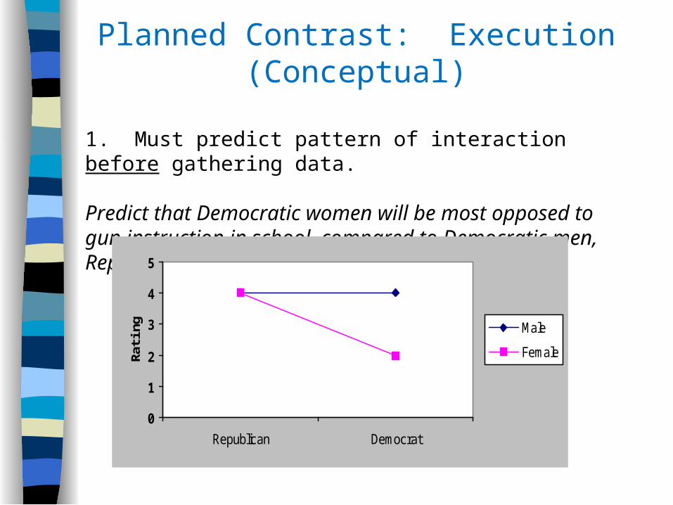
Planned Contrast: Execution (Conceptual)

1. Must predict pattern of interaction before gathering data. Predict that Democratic women will be most opposed to gun instruction in school, compared to Democratic men, Republican men, and Republican women.

0

1

2

3

4

5

Republican Democrat

Rat

ing Male

Female

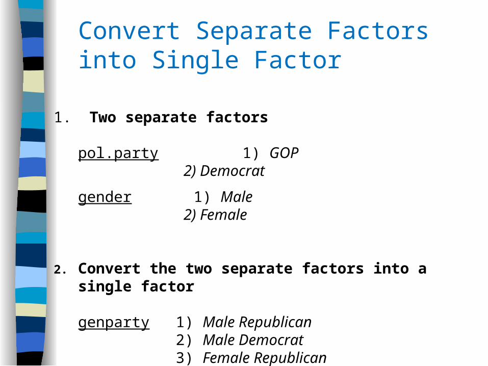
Convert Separate Factors into Single Factor

1. Two separate factors

pol.party 1) GOP 2) Democrat

gender 1) Male 2) Female

2. Convert the two separate factors into a single factor

genparty1) Male Republican2) Male Democrat3) Female Republican4) Female Democrat

Convert Separate Factors into Single FactorSPSS Syntax (commands)

genparty1 = Male Republican2 = Male Democrat3 = Female Republican4 = Female Democrat

Converting Multi-factors into Single Factor for Planned Contrast

Political Party Male Female

Republican 5.00 4.75

Democrat 4.50 2.75

Gender

Converted into single factor with four levels

GENPARTY

1 = Male/Republican 5.002 = Male/Democrat 4.503 = Female/Republican 4.754 = Female/Democrat 2.75

Planned Contrast: Execution (Conceptual) 3. Conduct one-way ANOVA, with new single variable as predictor.

4. Assign weights to the four levels, as follows:

1) Male Republican -12) Male Democrat -13) Female Republican -14) Female Democrat 3

* Weights indicate which sub-groups are to be compared. * Weights must add up to zero

5. Planned contrast then limits comparison to the indicated groups, but “counts” all subjects in terms of degrees of freedom and computation of error. This provides greater predictive power. This is even true if weight for some group(s) set at zero.

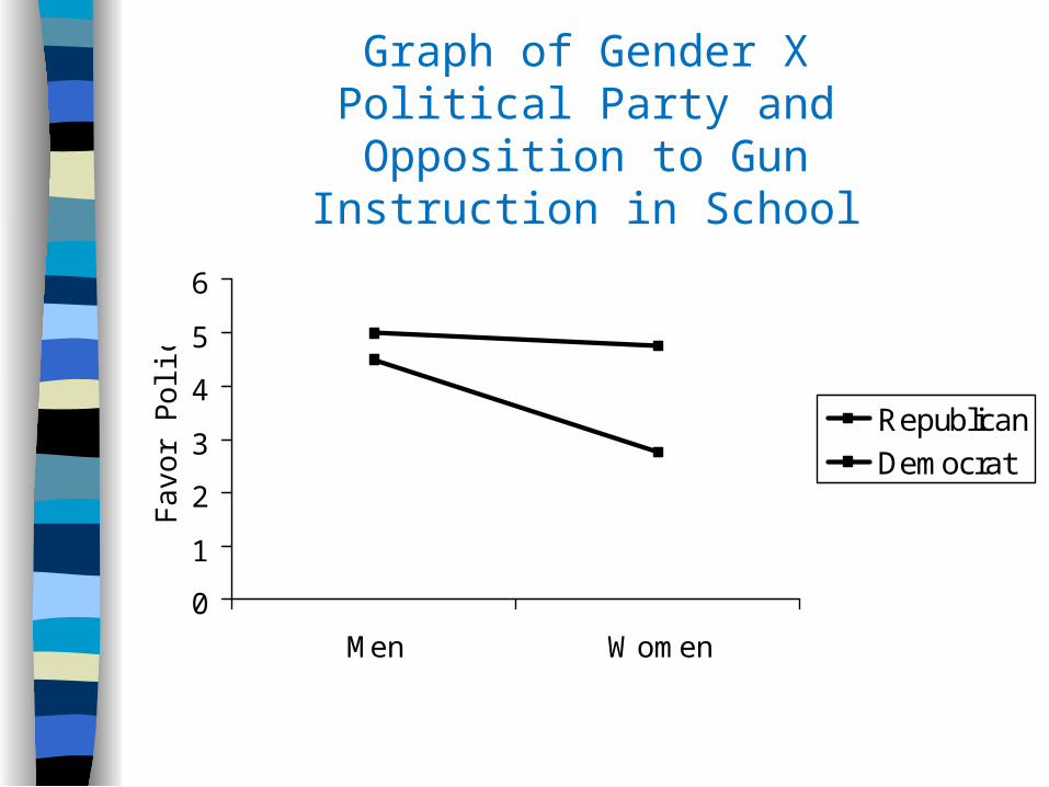
Graph of Gender X Political Party and Opposition to Gun Instruction in School

0

1

2

3

4

5

6

Men Women

Fa

vor

Po

licy

Republican

Democrat

Univariate Analysis of Variance [DataSet1] Descriptive Statistics

Dependent Variable: gunctrl

5.0000 .81650 4

4.5000 1.29099 4

4.7500 1.03510 8

4.7500 .95743 4

2.7500 .95743 4

3.7500 1.38873 8

4.8750 .83452 8

3.6250 1.40789 8

4.2500 1.29099 16

partyrepublican

democrat

Total

republican

democrat

Total

republican

democrat

Total

gendermale

female

Total

Mean Std. Deviation N

Tests of Between-Subjects Effects

Dependent Variable: gunctrl

12.500a 3 4.167 4.000 .035

289.000 1 289.000 277.440 .000

4.000 1 4.000 3.840 .074

6.250 1 6.250 6.000 .031

2.250 1 2.250 2.160 .167

12.500 12 1.042

314.000 16

25.000 15

SourceCorrected Model

Intercept

gender

party

gender * party

Error

Total

Corrected Total

Type III Sumof Squares df Mean Square F Sig.

R Squared = .500 (Adjusted R Squared = .375)a.

Orthogonal Interaction

Descriptives

gunctrl

4 5.0000 .81650 .40825 3.7008 6.2992 4.00 6.00

4 4.5000 1.29099 .64550 2.4457 6.5543 3.00 6.00

4 4.7500 .95743 .47871 3.2265 6.2735 4.00 6.00

4 2.7500 .95743 .47871 1.2265 4.2735 2.00 4.00

16 4.2500 1.29099 .32275 3.5621 4.9379 2.00 6.00

male republican

male democrat

female republican

female democrat

Total

N Mean Std. Deviation Std. Error Lower Bound Upper Bound

95% Confidence Interval forMean

Minimum Maximum

ANOVA

gunctrl

12.500 3 4.167 4.000 .035

12.500 12 1.042

25.000 15

Between Groups

Within Groups

Total

Sum ofSquares df Mean Square F Sig.

Planned Contrast, Page 1

Note: This is ANOVA p value, NOT contrast p value

Contrast Coefficients

-1 -1 -1 3Contrast1

malerepublican

maledemocrat

femalerepublican

femaledemocrat

genparty

Planned Contrast, Page 2

Contrast Tests

Contrast

Assumes eq. var.

Doesn’t assume eq. var.

Contrast value

-6.000

-6.000

Std.Error

1.768

1.696

-3.394

-3.539

12

5.501

.005

.014

t df Sig. (2 –tailed)

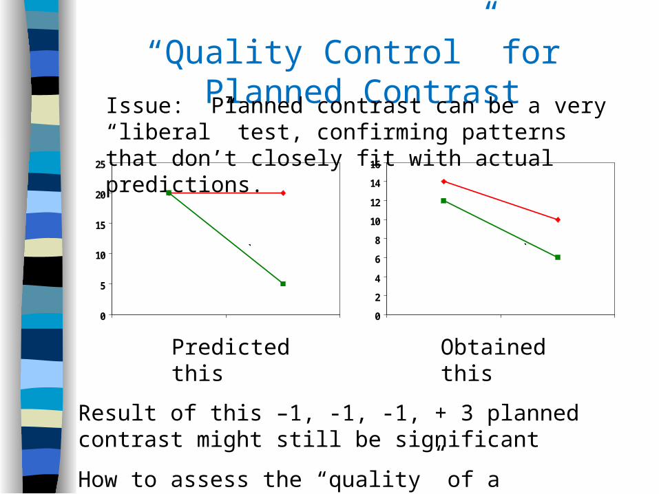
“Quality Control” for Planned ContrastIssue: Planned contrast can be a very “liberal” test, confirming patterns that don’t closely fit with actual predictions.

Predicted this Obtained this

Result of this –1, -1, -1, + 3 planned contrast might still be significant

How to assess the “quality” of a significant planned contrast?

0

5

10

15

20

25

`

0

2

4

6

8

10

12

14

16

`

Analysis of Residual Variance

Logic of test:

Did (Between groups effect – Contrast effect) leave significant amount of systematic (non-random) variance unexplained?

If so, then the contrast did not do a good job. It did not explain the outcome fully.

However, if “what’s left over” (i.e., between effect – contrast) is not significant, then the contrast accounts for most of thetreatment.

In this case, the contrast did do a good job.

Contrast Should “Absorb” Most of Between-Groups Effect

─ ═

Between Groups

Variance

Contrast Effect

Remaining Variance

Steps in Analysis of Residual Variance Test

1. Get SPSS printout of planned contrast

2. Get t of contrast, square it to get contrast F (t = F )

3. Compute SS contrast (SSc): Multiply contrast F by mean sq. w/n (MSw) of oneway ANOVA. This results in SS contrast (SSc).

4. Compute SS residuals (SSr): Get SS between (SSb) from oneway, and subtract SSc. (SSb – SSc) = SS residuals (SSr)

5. Compute MS contrast (MSc): Divide SSr by df, which is (oneway df – planned contrast df). This produces the MS contrast (MSc)

6. Compute F residuals: Divide MSc by MSw. MSc/MSw = F residuals

7. Compute df for F resid: numerator df = (df oneway – df contrast; see 5, above), denominator df = df within (from oneway).

8. Check this F in F table from any stats book. If significant, contrast is not a good fit. If not significant, the contrast is a good fit.

Residuals Analysis Test

1. Get SPSS printout of planned contrast

2. F of contrast (Fcont) = t2; t = -3.39 t2 = 11.49

3. SScontrast (SScont): F cont X MSw = 11.49 X 1.04 = 11.95

4. SSresiduals (SSres): SSbetween (SSb) = 12.50

SSb – SScont = 12.50 – 11.95 = .55

5a. Contrast df = df oneway – df contrast = 15 -12 = 3

5b. MScontrast (MScont) = SSres / contrast df = .55/3 = 0.18

6. F residuals (Fresid): Divide MScont by MSw = 0.18/1.04 = .17

7. DF for Fresid = df contrast (see 5a, above), df within: (3, 12)

8. F table at (3, 12) df, for criterion p < .25; F = 1.56

9. Obtained Fresid = 0.17 < 1.56, therefore residual is not significant, therefore contrast result is a good fit for data.

Post Hoc Tests

Do female democrats differ from other groups?

1 = Male/Republican 5.002 = Male/Democrat 4.503 = Female/Republican 4.754 = Female/Democrat 2.75

Conduct three t tests? NO. Why not? Will capitalizes on chance.

Solution: Post hoc tests of multiple comparisons.

Post hoc tests consider the inflated likelihood of Type I error

Kent's favorite—Tukey test of multiple comparisons, which is the most generous.

NOTE: Post hoc tests can be done on any multiple set of means, not only on planned contrasts.

Conducting Post Hoc Tests

1. Recode data from multiple factors into single factor, as per planned contrast. 2. Run oneway ANOVA statistic 3. Select "posthoc tests" option.

ONEWAY gunctrl BY genparty /CONTRAST= -1 -1 -1 3 /STATISTICS DESCRIPTIVES /MISSING ANALYSIS /POSTHOC = TUKEY ALPHA(.05).

Selected post-hoc test

Note: Not necessary to conduct planned contrast to conduct post-hoc test

Descriptives

gunctrl

4 5.0000 .81650 .40825 3.7008 6.2992 4.00 6.00

4 4.5000 1.29099 .64550 2.4457 6.5543 3.00 6.00

4 4.7500 .95743 .47871 3.2265 6.2735 4.00 6.00

4 2.7500 .95743 .47871 1.2265 4.2735 2.00 4.00

16 4.2500 1.29099 .32275 3.5621 4.9379 2.00 6.00

male republican

male democrat

female republican

female democrat

Total

N Mean Std. Deviation Std. Error Lower Bound Upper Bound

95% Confidence Interval forMean

Minimum Maximum

ANOVA

gunctrl

12.500 3 4.167 4.000 .035

12.500 12 1.042

25.000 15

Between Groups

Within Groups

Total

Sum ofSquares df Mean Square F Sig.

Post hoc Tests, Page 1

Multiple Comparisons

Dependent Variable: gunctrl

Tukey HSD

.50000 .72169 .898 -1.6426 2.6426

.25000 .72169 .985 -1.8926 2.3926

2.25000* .72169 .039 .1074 4.3926

-.50000 .72169 .898 -2.6426 1.6426

-.25000 .72169 .985 -2.3926 1.8926

1.75000 .72169 .125 -.3926 3.8926

-.25000 .72169 .985 -2.3926 1.8926

.25000 .72169 .985 -1.8926 2.3926

2.00000 .72169 .070 -.1426 4.1426

-2.25000* .72169 .039 -4.3926 -.1074

-1.75000 .72169 .125 -3.8926 .3926

-2.00000 .72169 .070 -4.1426 .1426

(J) genpartymale democrat

female republican

female democrat

male republican

female republican

female democrat

male republican

male democrat

female democrat

male republican

male democrat

female republican

(I) genpartymale republican

male democrat

female republican

female democrat

MeanDifference

(I-J) Std. Error Sig. Lower Bound Upper Bound

95% Confidence Interval

The mean difference is significant at the .05 level.*.

Post Hoc Tests, Page 2

Data Management Issues

Setting up data file

Checking accuracy of data

Disposition of data Why obsess on these details? Murphy's Law

If something can go wrong, it will go wrong, and at the worst possible time.

Errars Happin!

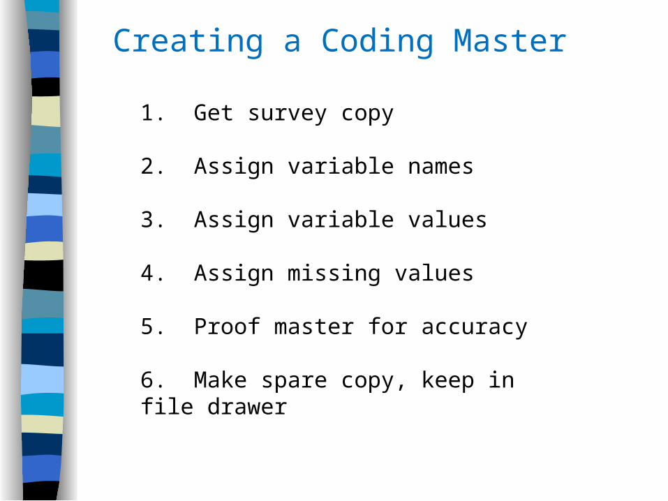
Creating a Coding Master

1. Get survey copy 2. Assign variable names 3. Assign variable values 4. Assign missing values 5. Proof master for accuracy 6. Make spare copy, keep in file drawer

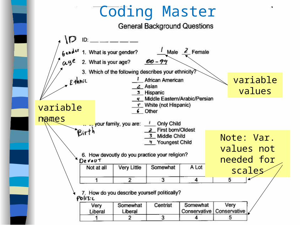
Coding Master

variable names

variable values

Note: Var. values not needed for scales

Cleaning Data Set

1. Exercise in delay of gratification 2. Purpose: Reduce random error 3. Improve power of inferential stats.

Complete Data Set

Note: Are any cases missing data?

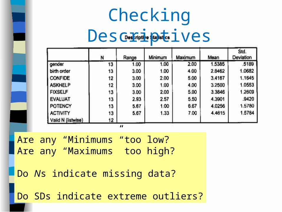
Are any “Minimums” too low? Are any “Maximums” too high?

Do Ns indicate missing data?

Do SDs indicate extreme outliers?

Checking Descriptives

Do variables correlate in the expected manner?

Checking Correlations Between Variables

Using Cross Tabs to Check for Missing or Erroneous Data Entry

Case A: Expect equal cell sizesGender 

Oldest Youngest Only Child

Males 10 10 20

Females 5 15 20

TOTAL 15 25 40

Case B: Impossible outcomeNumber of Siblings 

Oldest Youngest Only Child

None 4 3 6

One 3 4 0

More than one 3 4 2

TOTAL 10 10 8

Storing Data

Raw Data

1. Hold raw data in secure place

2. File raw data by ID #

3. Hold raw date for at least 5 years post publication, per APA Automated Data

1. One pristine source, one working file, one syntax file

2. Back up, Back up, Back up

` 3. Use external hard drive as back-up for PC

File Raw Data Records By ID Number

01-20 21-40 41-60 61-80 81-100 101-120

COMMENT SYNTAX FILE GUN CONTROL STUDY SPRING 2007

COMMENT DATA MANAGEMENT

IF (gender = 1 & party = 1) genparty = 1 .EXECUTE .IF (gender = 1 & party = 2) genparty = 2 .EXECUTE .IF (gender = 2 & party = 1) genparty = 3 .EXECUTE .IF (gender = 2 & party = 2) genparty = 4 .EXECUTE .

COMMENT ANALYSES

UNIANOVA gunctrl BY gender party /METHOD = SSTYPE(3) /INTERCEPT = INCLUDE /PRINT = DESCRIPTIVE /CRITERIA = ALPHA(.05) /DESIGN = gender party gender*party .

ONEWAY gunctrl BY genparty /CONTRAST= -1 -1 -1 3 /STATISTICS DESCRIPTIVES /MISSING ANALYSIS /POSTHOC = TUKEY ALPHA(.05).

Save Syntax File!!!

Research Project NotebookPurpose: All-in-one handy summary of research project

Content: 1. Administrative (timeline, list of staff, etc.)2. Overview3. Experiment Materials

* Surveys* Consents, debriefings* Manipulations* Procedures summary/instructions

4. IRB materials* Application* Approval

5. Data* Coding forms* Syntax file* Primary outcomes