planning as refinement search: a unified framework for

Planning as Refinement Search: A unified framework forcomparative analysis of Search Space Size and

Performance

Subbarao Kambhampati�

Department of Computer Science and EngineeringArizona State University, Tempe, AZ 85287-5406

Email: [email protected]

ASU CSE Technical Report 93-004June, 1993

AbstractIn spite of the long history of classical planning, there has been very little comparative analysis

of the search space characteristics of the multitude of existing planning algorithms. This hasseriously inhibited efforts to fruitfully intergrate various approaches. In this paper we show thatviewing planning as a general refinement search provides a unified framework for comparing thesearch spaces of various planning strategies, and in predicting their performance. We will providea generic refinement search algorithm for planning, and show that all planners that search in thespace of plans are special cases of this algorithm. In this process, we will provide a rationalreconstruction of main ideas of refinement planning algorithms. We will then develop a model forestimating search space size of a refinement planner, and use this model to analyze a variety oftradeoffs between search space size, refinement cost and performance in refinement planning.

�This research is supported in part by National Science Foundation under grant IRI-9210997, and ARPA/RomeLaboratory planning initiative under grant F30602-93-C-0039.

0

1 Introduction

[...] Search is usually given little attention in this field, relegated to a footnoteabout how ‘‘Backtracking was used when the heuristics didn’t work.’’

Drew McDermott, [12, p. 413]

The idea of generating plans by searching in the space of (partially ordered or totally ordered)plans has been around for almost twenty years, and has received a lot of formalization in the pastfew years. Much of this formalization has however been limited to providing semantics for plansand actions, and proving soundness and completeness of planning algorithms. There has beenvery little comparative analysis of the search space characteristics of the multitude of existingclassical planning algorithms. There is a considerable amount of disagreement and confusion onthe role and utility of even such long-standing concepts as ‘‘goal protection’’, and ‘‘protectionintervals’’ -- not to mention the more recent ideas such as ‘‘systematicity’’ -- on the search spacecharacteristics of planning algorithms. One reason for this state of affairs is the seemingly differentvocabularies and/or frameworks within which many of the algorithms are usually expressed. Thelack of a unified framework for viewing planning algorithms has hampered comparative analyses,which in turn has severely inhibited fruitful integration of competing approaches.1

In this paper, we shall show that viewing planning as a refinement search provides a unifiedframework within which a variety of refinement planning algorithms can be effectively compared.We will start by characterizing planning as a refinement search, and provide semantics for partialplans and plan refinement operations. We will then provide a generic refinement planningalgorithm in terms of which the whole gamut of the so-called plan-space planners, which search inthe space of partial plans, can be expressed. We will use this unifying model to provide a rationalreconstruction of main ideas of refinement planning algorithms. This reconstruction facilitatesseparation of important ideas underlying individual algorithms from ‘‘brand-names’’, and thusprovides a rational basis for fruitfully integrating the various approaches. Finally, we develop amodel for estimating the search space size of a refinement planner, and use it to analyze the tradeoffsprovided by many approaches for improving performance by reducing search space size. As ourmodel does not assume any restrictions on action representations, it also facilitates evaluation ofthese approaches terms of their ability to scale up to more expressive action representations.

This paper is organized as follows: Section 2 reviews the objectives of classical planning,and defines the notions of solutions and completeness. Section 3 introduces general refinementsearch, and characterizes planning as a refinement search. It also provides semantics for partialplans in terms of refinement search, and develops a generic algorithm for refinement planning. InSection 4, this generic algorithm is used as a backdrop to provide a rational reconstruction of themain ideas of existing refinement planners. Particular attention is paid to the variety of techniques

1The work of Barrett and Weld [24] as well as Minton et. al. [15, 16] are certainly steps in the right direction.However, they do not tell the full story since the comparison there was between a specific partial order and total orderplanner. The comparison between different partial order planners itself is still largely unexplored.

1

used by planners to avoid looping, redundancy and non-minimal plans. Section 5 provides aqualitative model for estimating search space size of refinement planners, and uses it to analyzethe tradeoffs provided by a variety of approaches for improving performance through search spacereduction, including ‘‘systematicity’’, ‘‘strong systematicity’’, and ‘‘conflict deferment’’. Section6 summarizes the contributions of the paper and discusses potential applications of the frameworkfor refinement planning developed in this paper. Related work is discussed throughout the paperat appropriate places.

2 Goals, Solutions and Completeness in classical planning

Whatever the exact nature of the planner the ultimate aim of (classical) planning is to find a groundoperator sequence, which when executed will produce desired behaviors or sequences of worldstates. Thus, goals of planning should be seen as specifications on the desired behaviors (e.g. aspredicates on state sequences). A planning problem is thus specified by providing the descriptionof the initial state, and a specification of behavioral constraints. Most classical planning techniqueshave traditionally concentrated on the sub-class of goals called the goals of attainment, whichessentially constrain the agent’s attention to behaviors that end in world states satisfying desiredproperties. Unless otherwise stated, this is the class of goals we shall also be considering in thispaper.

The operators (aka actions) in classical planning are modeled as general state transformationfunctions. We will be assuming that the domain operators are described in STRIPS representationwith Add, Delete and Precondition formulas. The subset of this representation where all threeformulas can be represented as conjunctions of function-less first order literals, and all the variableshave infinite domains, will be referred to as TWEAK representation (c.f. [1, 9]).

Given this vocabulary, a solution for a planning problem can be formally defined as:

Definition 1 (Solution) A ground operator sequence S : o1; o2; � � � on is said to be a solution to aplanning problem [I;G], where I is the initial state of the world, and G is the specification of thedesired behaviors, if (i) if S is executable, i.e.,

I ` prec(o1)

o1(I) ` prec(o2)

� � �

on�1(on�2 � � � (o1(I))) ` prec(on)

(where prec(o) denotes the precondition formula of the operator o) and (ii) the sequence of statesI; o1(I); � � � ; on(on�i � � � (o1(I))) satisfies the behavioral constraints specified in the planning

2

goals. For goals of attainment, this latter requirement is stated solely in terms of the last stateresulting from the plan execution:

on(on�i � � � (o1(I))) ` G

The definition of solution, given above, admits many redundant operator sequences as solutions.Suppose we are interested in goals of attainment, and the operator sequence S is a solution. From S

it is possible to derive potentially infinite number of other solutions by adding additional operatorswhich are executable, and do not interact with the existing operators of S. The presence of suchredundant solutions necessitates focus on minimal solutions:

Definition 2 (Minimal Solutions) A solution S is said to be minimal,2 if no operator sequenceobtained by removing some of the steps from S is also a solution.

A specific type of non-minimal solutions, called ‘‘bloated solutions,’’ are of particular interest(see below):

Definition 3 (Bloated Solutions) A solution S is said to be bloated (c.f. [12]) if the operatorsequence S0 obtained by deleting some operator o 2 S, is also a solution. A solution that is notbloated is called an un-bloated solution.

(Note that un-bloated solutions are not necessarily minimal; it may be possible to removea non-singleton set of steps from them, while still keeping them as a solution.) Completenessresults for classical planners are typically stated and proved with respect to some class of minimalsolutions.3:

Definition 4 (Completeness) A planner is said to be complete if it can find all minimal solutionsfor every solvable problem.

Many planners described in the literature are in fact complete for the larger class of unbloatedsolutions [23, 12]. Despite the statement of completeness results in terms of minimal plans,the search spaces of most classical planners do however contain bloated solutions; the extent ofbloated plan generation does vary from planner to planner. We will see that the desire to avoidplanning decisions that lead to non-minimal solutions, is one of the implicit driving forces behindthe development of many important ideas in planning algorithms.

2Notice that minimal solutions are defined with respect to the solution criterion. For example, in most classicalplanning systems dealing with goals of attainment, any solution which gives rise to state-cycles (e.g. the sequence ofactions Open the door, Close the door one after other lead us back to the same state) are non-minimal. However, if thegoal of the planner itself was to exhibit a behavior (state sequence) containing the same state more than once, theymay not be non-minimal.

3The definition of completeness with respect to all rather than a minimal solution is in a way ironic consideringthat most practical planners require only one solution for a given problem, and optimality of solutions has not been aprimary consideration in classical planning.

3

3 Planning as Refinement Search

Almost all classical planners that search in the space of plans use refinement search to navigatethe space of ground operator sequences and find a solution for the given planning problem. Arefinement search (or split-and-prune search [19]) can be visualized either as a process of startingwith a partial solution and adding detail to the partial solutions until it satisfies the solutionconstraints, or equivalently, as a process of starting with the set of all potential candidates, andsplitting the set repeatedly until a solution candidate can be picked up from one of the sets inbounded time.4 The set of all candidates for the refinement search is denoted by =. The denotationof a search node N in refinement search, written as [[N ]], is a subset of =. The denotation of theinitial search node is the set of all candidates, =.

In the case of planning, = is the set of all ground operator sequences. Suppose the domaincontains three ground actions a1, a2 and a3, then the regular expression fa1ja2ja3g� woulddescribe the potential solution space for this domain. Each search node corresponds to some subsetof these ground operator sequences.

Although it is conceptually simple to think of search nodes in refinement search in terms oftheir denotations (i.e, sets of potential candidates), we obviously do not want to represent thecandidate sets explicitly in our implementations. Instead, the candidate set is typically implicitlyrepresented as a generalized constraint set (c.f. [5] such that every potential candidate that isconsistent with the constraints in that set is taken to belong to the candidate set of the search node.(Because of this, search nodes in refinement search are often seen also as ‘‘partial solutions’’.)

3.1 Semantics of Partial Plans

In the case of planning, search nodes can be seen as a set of constraints defining partial plans (inthe following, we will be using the terms ‘‘search node’’ and ‘‘partial plan’’ interchangeably). Atan abstract level, the search-node (partial plan) representation used by all refinement planners canbe described in terms of a 5-tuple:

hT;O;B;ST ;Li

where:

� T is the set of actions (step-names) in the plan; T contains two distinguished step names tIand tG.

� ST is a symbol table, which maps step names to domain operators. It always maps thespecial step tI to the dummy operator start, and tG to the dummy operator fin. The

4Pearl defines termination conditions of a split-and-prune strategy in a slightly different manner, requiring that thethe set be split repeatedly until a singleton set containing a solution candidate is reached. The termination conditiondiscussed here is more general-- search terminates as soon as a set of candidates is generated from which the solutionconstructor function can pick a solution candidate. It allows the complexity to be shared between the solutionconstructor function and the children generator. (This idea was suggested by David McAllester).

4

effects of start and the preconditions of fin correspond to the initial and final states ofthe plan, respectively.

� O is a partial ordering relation over T . For the special case where O defines a total orderingon the steps of T , P is called a totally ordered plan.

� B is a set of codesignation (binding) and non-codesignation (prohibited bindings) constraintson the variables appearing in the preconditions and post-conditions of the operators.

� L is a set of auxiliary constraints on the orderings and bindings among the steps. Exampleof an auxiliary constraint that we shall see latter (Section 4.2.4)is a exhaustive causal link:5

fsgp! w where s;w 2 T and p 2 preconditions(w)

This constraint is interpreted as:

‘‘s comes before w and gives p to w. No other step in the plan is allowed tocome between s and w and add or delete p.’’

We shall now formally define the candidate set of a partial plan:

Definition 5 (Candidate set of a Partial plan) Given a search node N with the partial planP : hT;O;B;ST ;Li, a ground operator sequence S is said to belong to [[N ]] if and only if thereexists a partial mapping between the operators of S and steps of P such that S satisfies all theconstraints of P . That is, S contains the operators corresponding to all the steps of P (exceptingthe dummy steps start and finish) in an ordering that is consistent with O and bindingsconsistent with B, and S also satisfies the constraints of L.6

As an example, suppose the partial plan of the node N is given by the constraint set*ftI; t1; t2; tGg; ftI � t1; t1 � t2; t2 � tGg; ;;ft1 ! o1; t2 ! o2; tI ! start; tG ! finishg; ;

+

The ground operator sequence o1; o3; o2 is consistent with the constraints of the partial plan, andthus belongs to the candidate set of N . If the partial plan contains an exhaustive causal link (seeabove) as an auxiliary constraint:

5Auxiliary constraints can be more expressive than this. For example, an auxiliary constraint may express theconstraint that a particular step must always be in a specific absolute position in every candidate, or that a particularoperator must not come more than once in any candidate. The former can be used to model state based plannersthat allow step additions only at either end of the partial plan. The latter may be useful when dealing with planningsituations where not all goals are goals of attainment.

6It is helpful to think of L as a filter on the candidates that satisfy the other constraints of P.

5

*ftI ; t1; t2; tGg; ftI � t1; t1 � t2; t2 � tGg; ;;

ft1 ! o1; t2 ! o2; tI ! start; tG ! finishg; fft1gP! t2; ft2g

Q! tGg

+

Then, candidate (ground operator sequence) o1; o3; o2 is consistent with the constraints of thepartial plan, and thus belongs to the candidate set of N if and only if o3 does not have P as an addor delete literal. Similarly, the candidate o1; o2; o5 belongs to the candidate set of N if and only ifo5 does not add or delete Q.

Partial order vs. Total order planning: The only difference between partial order and total orderplanners are the extent of ordering in the partial plans. In total order planners, the partial planP : hT;O;B;ST ;Li of every search node is totally ordered (i.e., O defines a total ordering onT ), while in partial order planners it may be partially or totally ordered. The primary motivationbehind partial order planning is efficiency -- by deferring orderings among operators, partial orderplanners avoid premature commitment and the consequent unnecessary backtracking, therebyimproving performance [24, 9]. It is important to note that while partial order and total orderplanners use different representation constraints on the partial plans, the main goal of planning ineither case still remains finding a ground operator sequence that is executable and satisfies goalcriteria. In particular, partial order planners do not aim to find least constrained partially orderedoperator sequences. It is easy to see that a total ordering places more constraints on the partial planthan a partial ordering. Thus, all else being equal, the difference between a total ordering plannerand a corresponding partial ordering planner is merely that the candidate sets (denotations) of thethe former are on the average smaller than that of the latter. As we shall see latter, this tends toreduce the overall size of search space of partial order planners, while at the same time increasingthe cost of refinement in partial order planning. We will also see that from a refinement searchpoint of view, partial order planning is more natural than total order planning. The motivations forthe latter come in terms of the refinement cost.

Ground Linearizations and Candidate sets: As mentioned earlier, partial plans can also be seenas partial solutions to the planning problems. Previous formalizations of refinement planning,especially that of Chapman’s TWEAK, took this approach and discussed notions of correctnessof partial plans. At this point, it is useful to introduce some of that terminology and relate it tocandidate set based semantics of partial plans.

Definition 6 (Ground Linearizations and Safe Ground Linearizations) A ground lineariza-tion (aka completion) of a partial plan P :hT;O;B;ST ;Li is a fully instantiated total ordering ofthe steps of P that is consistent with O (i.e., a topological sort) and B.

A ground linearization is said to be a safe ground linearization if and only if it alsosatisfies all the auxiliary constraints.

For the example plan

6


ft1 ! o1; t2 ! o2; tI ! start; tG ! finishg; fft1gP! t2; ft2g

Q! tGg

+

discussed above, tIt1t2tG is the only ground linearization, and it is also a safe ground linearization.Note that safe ground linearizations are related to minimal candidates in the following sense:

Proposition 1 (Candidate Sets and Safe Ground Linearizations) Every candidate S belongingto the candidate set of a node N : P : hT;O;B;ST ;Li is either a minimal candidate, in thatit exactly matches a safe ground linearization of N (except for the dummy steps tI and tG, andmodulo the mapping of ST ), or is a safe augmentation of a minimal candidate obtained by addingadditional ground operators without violating any auxiliary constraints.

Once again, for our example plan above, o1o2 is a minimal candidate because it exactly matchesthe safe ground linearization tIt1t2tG, under the mapping ST . The ground operator sequenceo1o3o2o4, where o3 does not add or delete P , and o4 does not add or delete Q, is a candidate of thisplan. It can be obtained by augmenting the minimal candidate o1o2 with the ground operators o3

and o4 without violating auxiliary constraints.We will now define the notion of consistency of a partial plan/search node:

Definition 7 (Consistency of search nodes) A search node is consistent if it has a non-emptycandidate set (or alternately, the set of constraints in the search nodes are satisfiable).

Nodes with empty candidate sets obviously cannot lead to a solution candidate and thus mustbe pruned. Given the relation between safe ground linearizations and candidate sets of a partialplan, it follows that:

Proposition 2 A search node in refinement planning is consistent if and only if the correspondingpartial plan has at least one safe ground linearization.

We will also define a related planning-specific notion called safety of partial plans, which willbe useful in discussing conflict resolution strategies used by many refinement planners:

Definition 8 (Safety of partial plans) A partial plan is said to be safe if all its ground lineariza-tions are safe

It is easy to see that safety of partial plans is a stronger constraint than consistency.

Correctness of conditions w.r.t. ground linearizations: For the special case of goals ofattainment, the correctness of a partial plan can be defined solely in terms of establishment of thepreconditions of all the steps in the plan. A precondition of a partial plan P : hT;O;B;ST ;Li is atwo tuple hC;ni, where n 2 T , and C is a precondition of n. hC;ni is said to be true in a ground

7

linearization of P , if there is a step n0 which comes before n in the total ordering and n has aneffect C , and no step between n0 and n deletes C . If hC;ni is not true, then it is false in that groundlinearization. hC;ni is said to be necessarily true in P if it is true in every ground linearizationof P . It is said to be necessarily false if it is false in every ground linearization of P . In manyinstances hC;ni is neither necessarily true, nor necessarily false; in this case we call it possiblytrue7 (i.e., it is true in some ground linearizations and false in others).

Chapman’s definition of correctness of partial plans can be cast in our terminology as:

Definition 9 (Partial plan correctness) A partial plan is said to be correct if and only if eachof its ground linearizations exactly matches a solution candidate for the problem (modulo themapping in ST ).

3.2 A generic algorithm template for refinement planning

A refinement search is specified by providing a set of refinement operators (strategies) R, anda constructor function sol. The search process starts with the initial node �, and consists ofgenerating children nodes by application of refinement operators. A refinement operator (strategy)R 2 R is a function that maps subsets of = (the set of all candidates) to sets of subsets of =, suchthat if a subset s � = is mapped to the set of subsets fs1; s2 � � � sng, then 8i si � s. Refinementoperators can thus be seen as set splitting operations on the candidate sets of search nodes -- theymap a search node N to a set of children nodes fN 0

ig such that 8i [[N 0i ]] � [[N ]]. Another

example of an auxiliary constraint may be that a particular operator must not come more than oncein any candidate.

Definition 10 (Completeness and Systematicity of a Refinement Strategy) Let R be a refimentstrategy that maps a node N to a set of children nodes fN 0

ig. R is said to be complete ifSi[[N

0i ]] � [[N ]] (i.e., no candidate is lost in the process of refinement).

R is said to be systematic if 8N 0

i;N 0

j[[N 0

i ]] \ [[N 0j]] � ;.

The search process involves selecting a candidate set and refining it (splitting it) into subsets.The search terminates when a node n is found for which the constructor function returns a solutioncandidate. A constructor function (aka solution constructor function) sol is a 2-place functionwhich takes a search node and a solution criterion as arguments. It may return either one of threevalues:

1. *fail*, meaning that no candidate in [[N ]] satisfies solution criterion

2. Some candidate c 2 [[N ]] which satisfies the solution criterion (i.e., c is a solution candidate)

7Note that the notion of ‘‘truth’’ here is conditional on executability. Just because a condition hC; ni is necessarilytrue, it doesn’t mean that some ground linearization of P can be executed to produce C before n. See [9] for furtherdiscussion on this distinction.

8

Algorithm: Refinement Search(sol;R)1. Initialize Search queue with �, the node with null constraint set

Begin Loop2. If search queue is empty, terminate with failure3. Else, non-deterministically pick a node n from the search queue4. If sol(n,G) returns a candidate c, return it with success5. Else, choose some refinement operator R 2 R,

(Not a backtrack point.)6. generate R(n), the refinements of n with respect to R.7. Prune any nodes in R(n) that are inconsistent.8. Add the remaining nodes in R(n) to the search queue.

End Loop

Figure 1: A generic Refinement search strategy

3. ?, meaning that sol can neither construct a solution candidate, nor determine that no suchcandidate exists.

In the first case, N will be pruned. In the second case search terminates with success, and inthe third, N will have to be refined further.

N is called a solution node if the call sol(N ;G) returns a solution candidate. Given thesedefinitions, the algorithm template in Figure 1 describes the general refinement search strategy8. Arefinement search is complete, in the technical sense that it will find a solution candidate eventuallyif one exists, as long as all of its refinement strategies are complete (see above).

The procedure Find-plan in Figure 2 and the procedure Refine-Plan in Figure 3instantiate the refinement search within the context of planning. In particular, they describea generic refiment-planning algorithm, which can be specific instantiations of which cover thecomplete gamut of refinement planners, including partial ordering, total ordering, unambiguous,

8While there are several similarities between this algorithm and classical branch and bound search algorithm [17],there is one important difference worth noting: Branch and bound search typically assumes that all the candidates aresolutions, and searches for an optimal solution candidate. Thus, the pruning part in line 7 of the refinement searchalgorithm in Figure 1 is similar to, but weaker than the pruning criteria used in branch and bound algorithms [17]. Byreplacing line 7 with a pruning criterion that prunes nodes such that the cost of the best possible solution candidate intheir denotation is provably larger than the cost of best possible solution candidates in other nodes, we get branch andbound algorithm.

9

causal-link based, systematic, etc. The procedures are modular in that individual steps can beanalyzed and instantiated relatively independently. Furthermore, the algorithm itself does notassume any specific restrictions on action representation. The procedures thus provide a uniformbasis for understanding and comparing various planning algorithms in terms of search space sizeand performance.

The procedure Refine-Plan specifies the refinement operations done by the planningalgorithm. The goal selection step picks a goal to work on next. The establishment step enumeratesall possible ways of establishing the selected goal and generates one refinement (partial plan) foreach establishment choice. The book keeping step adds auxiliary constraints to each partial plan,to avoid violating this establishment decision in latter refinements. The consistency check stepchecks to see if each refinement (partial plan) is consistent (i.e., has non-empty candidate set). Insome sense, these are the only required steps. The refinement stops when the solution constructionfunction (in Find-Plan procedure) can construct a solution candidate from the search node itpicks for refinement.

An important consideration in refinement planning is cost of refinement. Complete consistencycheck turns out to be NP-hard for most common auxiliary constraints, making refinement costnon-polynomial. When the satisfiability of a set of constraints is intractable, we can still achievepolynomial refinement cost by refining the partial plans into a set of mutually exclusive andexhaustive constraint sets such that the consistency of each of those refinements can be checkedin polynomial time. It is to this end that some planners use either a pre-ordering step (such astotal ordering), or a conflict resolution step. The net effect of both these steps is to further refinethe refinements generated by the establishment step, by adding additional ordering and bindingconstraints, until the consistency of each refinement can be checked with cheaper (polynomialtime) consistency checks (see next section). In contrast to conflict resolution step, which isexplicitly geared towards consistency check, pre-ordering is in general geared towards makinghandling of partial plan, including consistency check and truth criterion interpretation, tractable.

From the description, it is clear that refinement (or candidate set splitting) is done in threedifferent stages-- as a part of establishment of new goals (we call this the establishment refinement),in pre-ordering the plan (called pre-ordering refinement), and in conflict resolution (called conflict-resolution refinement). In each refinement strategy, the added constraints include step addition,ordering addition, binding addition, as well as addition of auxiliary constraints. Although, for thesake of exposition the algorithm is written with the three refinement strategies in a particular serialorder, they can be done in any particular order. Conceptually, we can imagine the planner’s mainsearch loop to consist of picking a partial plan from the search queue, picking one of the refinementstrategies, and generating refinements of the partial plan with respect to that refinement, pruninginconsistent refinements. The planner will never have to backtrack on the choice of refinementstrategies -- the completeness of the algorithm will be preserved irrespective of the order in whichthe individual refinements are employed.

As we shall discuss in the next section, the traditional instantiations of all three individualrefinement strategies (see below) can be shown to be complete in that every ground operator

10

Algorithm Find-Plan(I;G)Parameters: sol: Solution constructor function.

1. Construct the null plan P; : hftI ; tGg; ftI � tGg; ;; ftI ! start; tG ! finishg; ; ;i, where tIis a dummy action with no preconditions, and the assertions in I as its effects, and tG is a dummyaction with no effects, and the assertions in G as the effects.

2. Initialize search queue with P;

3. Begin Loop

(a) Nondeterministically pick a node N with a corresponding partial plan P from the searchqueue.

(b) If sol(P) returns a solution, return it, and terminate.

(c) If sol(P) returns �fail�, skip to Step 3a.

(d) Call Refine-plan(P) (See Figure 3) to generate refinements of P .

(e) Add all the refinements to the search queue; Go back to 3a.

End Loop

Figure 2: A generic planning algorithm for refinement planning: Initial Call

sequence belonging to the candidate set of the parent plan will be a candidate of at least one ofthe refinements generated by each refinement strategy. Thus, all instantiations of refine-planwith these refinement strategies are also complete in the following technical sense: If there is asolution candidate in the candidate set of the initial (null plan), and if the solution constructorfunction is capable of picking that solution candidate given a sufficiently refined candidate setcontaining it, then any instantiation of Refine-Plan, with such a solution constructor function,will eventually terminate with success under all admissible search regimes.

.

4 A Rational Reconstruction of main ideas of Refinement Plan-ning

In this section, we shall use the generic refinement planning algorithm formulated in the previoussection as a backdrop to provide a rational reconstruction of some of the main ideas of refinement

11

Algorithm Refine-Plan(P)Parameters: pick-open: the routine for picking open conditions. pre-order: the routine whichadds orderings to the plan to make conflict resolution tractable. conflict-resolve:the routine whichresolves conflicts with auxiliary constraints.

1. Goal Selection: Using the pick-open function, pick an open goal hC; ni (where C is a preconditionof node n) from P to work on. Not a backtrack point (See Section 4.1.1)

2.1. Goal Establishment: Non-deterministically select an establisher step n0 for hC; ni. Introduce enoughconstraints into the plan such that (i) n0 will make C true, and (ii) C will persist until n. n mayeither already be in the plan, or may be a new step introduced into the plan. Backtrack point; allestablishers need to be considered (See Section 4.1)

2.2. Book Keeping: Add auxiliary constraints noting the establishment decisions, to ensure that thesedecisions are not violated by latter refinements. The auxiliary constraints may be one of goalprotection, protection intervals or contributor protection. (see Section 4.2)

3. Refinements to make plan handling/consistency check tractable (Optional) This step further refinesthe refinements generated by establishment decision.

3.a. Pre-Ordering: Use some static mechanism to impose additional orderings between steps of therefinements generated by the establishment check, with the objective of making handling ofthe partial plan (including consistency check, truth criterion interpretation) tractable Backtrackpoint; all interaction orderings need to be considered. (See Section 4.3.1)

OR

3.b. Conflict Resolution: Add orderings and bindings to resolve conflicts between the steps of theplan, and the plan’s auxiliary constraints. Backtrack point; all possible conflict resolutionconstraints need to considered. (See Section 4.3.2)

5. Consistency Check: If the partial plan is consistent, return it. If it is inconsistent (i.e., has no safeground linearizations), prune it. (See Section 4.3).

Figure 3: A generic algorithms for refinement planning: Refinement Procedure

12

planning algorithms. We will pay special attention to the search space characteristics. Unlessspecifically stated otherwise, for ease of exposition, we will be addressing the refinement of groundpartial plans.

4.1 Establishment

The most fundamental refinement operation is the so-called establishment operation. This consistsof adding constraints to the partial plan to establish some open condition hC;ni of the plan, whereC is a precondition of step n in the partial plan of the search node. Establishments can be donewith the help of existing steps in the plan (aka simple establishment), or by adding a new step tothe plan (aka step addition). In either case, establishment introduces new subgoals (in the formof the preconditions and secondary preconditions of the steps taking part in establishment; seebelow), as well as new ordering and binding constraints. The process continues until all open goalsare established.

First formalizations of refinement planning (e.g. [27, 1]) assumed that goal establishmentrequires ability to check the truth of arbitrary conditions in partial order plans. The Q&A procedurein Tate’s Nonlin [27], provided the first formal specification of necessary and sufficient conditionsfor ensuring the truth of a proposition in a ground partially ordered plan. Later work by Chapman’sTWEAK [1], extended this truth criterion to partially ordered partially instantiated plans. (see[1, 9] for more details). The truth criteria provide a way of checking the executability of a plan(and, for goals of attainment, also provide a way of checking goal satisfaction). When a particularcondition is not true, the establishment step adds enough constraints to make it necessarily true bythe truth criterion.

A problem with truth criterion based approaches is that interpreting truth-criterion becomesNP-hard for anything more expressive than TWEAK action representation.9 This makes refinementnon-polynomial. Since the objective of planning is to make a condition necessarily true, rather thancheck if a condition is necessarily true, it should be possible to avoid interpreting truth criterion,and just add sufficient constraints on the plan to ensure that the condition is necessarily true10,thus delegating all constraint satisfaction to the consistency check step. Pednault’s secondarypreconditions based theory of establishment [20, 21] was the first to formally advocate thisapproach. In Pednault’s theory, establishment essentially involves selecting some step n0 (eitherexisting or new) from the plan, and adding enough constraints to the plan such that (a) n0 � n

and (b) n0 causes C to be true after it (Pednault calls these causation preconditionsPC

n0) and (c)C is preserved by every step s0 possibly coming in between n0 and n (these are the preservationpreconditions

QCn ). For Tweak action representation, causation preconditions are expressible

as codesignation constraints among the variables of the plan, while preservation conditions areexpressible as non-codesignation constraints. For actions with conditional effects, causation and

9In fact, even within TWEAK representation, allowing finite-domain variables will make truth-criterion NP-hard10This essentially pushes the complexity into the consistency check.

13

preservation preconditions may also involve new subgoals at the corresponding steps. In that case,these subgoals are added to the list of open conditions that the planner has to work on.

4.1.1 Goal Selection

The establishment step assumes that the planner has selected a particular precondition of the planfor establishment in the current iteration. As far as the soundness and completeness of the planningalgorithm is concerned, the goal selection can be done in any arbitrary fashion, and a refinementplanner will never have to backtrack on the goal selection decision. There is a considerable amountof lee-way in selecting the goals. If precondition abstraction hierarchies are available, we can usethem to guide the selection. Even when such information is not available, there may be severalstatic goal ordering mechanisms. One particular static goal selection algorithm that is used inmany planners (such as UA and TWEAK) is to pick a goal that is not necessarily true. The costof this technique varies based on the nature of the partial plans maintained by the planner, and theexpressiveness of the action representation used. For unrestricted partially ordered plans containingactions with conditional effects, this goal selection strategy is NP-hard. For planners that maintainrestricted types of partial orderings, such as total orderings, or unambiguous orderings (c.f. [15];also see Section 4.3.1), this cost can be tractable. It is important to note that although in the pastdifferent ‘‘brand-name’’ planning algorithms have been associated with different goal selectionstrategies, the decision on which selection strategy to pick is relatively independent of the way restof the steps of the algorithm are instantiated. For example, there is no reason why SNLP cannotuse an MTC based goal selection strategy.

4.2 Book Keeping and Posting of Auxiliary Constraints

4.2.1 Motivation

It is possible to limit refinement to establishment operations alone and still get a sound and completeplanner. Chapman’s Tweak [1] is such a planner. It continues the establishment cycle until all thegoals and preconditions are necessarily true. Unfortunately, TWEAK turns out to have a lot ofredundancy in its search space. In particular, the example (a) in Figure 4 (originally from [15])shows that TWEAK may find the same solution candidate in multiple different search branches.(That is, the candidate sets of the search nodes in different branches overlap.) Furthermore, sinceTWEAK does not keep track of which goals it already achieved and which it is yet to achieve, itmay achieve and violate a goal/subgoal arbitrarily many times within the same refinement branch.This causes unnecessary looping and can generate many non-minimal solutions. Example (b) inFigure 4 shows a scenario where TWEAK repeatedly achieves and clobbers the conditions Q andR at action a1. In fact, in this example, TWEAK would loop infinitely if the action a4 is notavailable.

Although the presence of looping and non-minimal solutions in the search space is not somuch of a problem for planners using best-first search strategies and addressing solvable problems

14

(assuming that the ranking function takes into account the number of steps in the plan), it canbe much more problematic when the underlying search strategy is depth-first. In Example (b) ofFigure 4, a depth first search would have wasted a considerable amount effort on the loopingbranch, before reaching the depth bound and backtracking. This is where the book-keeping andconflict resolution steps comes in. Because the origins and motivations behind book keepingapproaches are generally misunderstood, in the following subsections, we will first provide arational reconstruction of the motivations behind the various approaches.

4.2.2 Book-keeping through Goal Protection

The looping behavior in the TWEAK example above could have been avoided had TWEAK kepttrack of the goals that it had already worked on, and avoided working on them again. In particular,suppose in a partial plan, the condition hC;niwhich has already been considered by TWEAK once,is seen to be necessarily false. In this case TWEAK can prune the plan without loss of completeness(i.e., no minimal solutions will be lost). The rationale is that when hC;ni was first considered,the planner would have considered all possible ways of establishing C at n, and thus pruning aplan where an already established condition is necessarily violated, does not affect completenessin terms of minimal solutions.11 This type of protection is known as goal protection. In terms ofthe refinement planning algorithm in Figure 3, goal protection adds an auxiliary constraint of theform hC;ni with the semantics that every candidate of the partial plan must have C true before n.

One way of implementing this book-keeping is to keep a list of closed-goals (i.e., goalswhich have already been considered by the establishment refinement step once), and whenever anew step is introduced into the plan, recheck to see if any of the closed-goals are possibly violated.If such ‘‘interactions’’ are discovered, then the planner could add additional orderings (constraints)to prune any unsafe ground linearizations (so that these linearizations will not be rechecked). Ifthis process leads to an inconsistent set of orderings, then the plan does not have any safe groundlinearizations, and thus can be pruned.

This technique for goal protection can be improved slightly-- rather than check for violationof every previously achieved goal on closed-goals list every time, we can keep track of theestablishment dependencies imposed at the time each goal hC;ni is made true, as a causal link

of the form fn0g C! n, where n0 is the step that was originally used to establish C at n. Whennew steps are introduced into the plan, we first check to see if the new step possibly violates thiscausal dependency (i.e., if it possibly comes in between n0 and n and deletes C). Only when thishappens, do we have to use the full-blown truth criterion to check whether or not C is necessarilytrue at step n. This is exactly the strategy followed by Tate’s Nonlin12 Nonlin maintained the

11This essentially bounds the maximum depth of the search space to be proportional to the number of preconditionsof the solution. Notice also that doing this does not avoid the looping problem completely. It is still possible to havelong chains of operators of type n0 and n00 such that n0 establishes C00 for n00, but needs C0 which can only be givenby n00; see below.

12In this paper, we will only be concentrating on the goal establishment and conflict resolution aspects of Nonlin,

15

causal dependencies in a structure called GOST, and used them to reduce the number of calls to thecostlier truth criterion (Q&A procedure).

An important, and often misunderstood ([14]) point to note about Nonlin’s strategy of keepingcausal links is that causal links were merely book-keeping devices for facilitating goal protection.From the planner’s point of view, the contributors of a causal link do not play any role in thesemantics of auxiliary constraints. In particular, suppose Nonlin finds that one of the causal linksof the current plan, fn0g C

! n, is violated, but the condition hC;ni itself is still true according toQ&A (presumably because of the effects of some other step n00 in the plan). In this case, Nonlinsimply replaces fn0g C! n with fn00g C! n and continues. Thus the causal link fn0g C! n doesnot preclude C from being violated in the interval hn0; ni. It merely implies that hC;ni has beenworked on once and the planner will ensure that it is not violated within this branch.13

4.2.3 Goal Protection by Protection Intervals

Although Nonlin does not use causal links as protection intervals, there have however been otherplanners, such as Pedestal [12], UCPOP [23], which do interpret a causal link fn0g C

! n as aprotection interval and consider any step s that can possibly intervene between n0 and n and deleteC as a threat (or conflict) that needs to be resolved by adding additional constraints to the partialplan. To understand this use of protection intervals, we have to recall that unlike TWEAK andNonlin, many planners do not explicitly use the truth criterion to check for goal protection. Amajor reason for this is that interpretation of a necessary and sufficient truth criterion is intractablefor actions more expressive than TWEAK action representation. Whenever a new step is added,checking to see if any of the previously achieved goals, or causal links, are violated will makerefinement intractable.14 Furthermore, since our ultimate goal is to avoid violating previouslyachieved goals (rather than merely checking if they are violated), we can avoid interpreting truthcriterion, and add constraints on the plan directly to ensure that newly added step preserves all thepreviously achieved goals. In Pednault’s terms, this involves adding preservation preconditions toensure that the new step will avoid violating the previously achieved goals.

Making the new step explicitly preserve all previously achieved goals is over-conservative andcan lead to loss of completeness. What we really want to do is to make the new step s preservea condition C if and only if C is required at some step n such that s comes possibly before n,and possibly after n0 (where n0 is an establisher of C). This is exactly where protection intervals

and ignore such additional features as hierarchical task reductions.13In some sense, this is as it should be. After all, since classical planning within STRIPS representation merely

needs that certain conditions be true at certain steps (the so-called ‘‘point protections’’), from the point of viewof soundness and completeness, there is no motivation for protecting a condition over a specific interval. (We areassuming that the planner is only interested in goals of attainment. The situation changes if we are also interested ingoals of maintenance: e.g.: Hold block ‘‘A’’ in the right hand, while stacking blocks ‘‘B’’ and ‘‘C’’ on ‘‘D’’ and ‘‘E’’respectively. Here, the protection intervals are necessary as a part of goal satisfaction.)

14Even Nonlin’s method of keeping causal links and checking if the new step violates the causal link is stillintractable for expressive action representations.

16

Figure 4: Examples showing redundancy and looping in TWEAK search space. In all the examples,the operators are shown with preconditions on the right side, and effects on the left (with ‘‘+’’sign for add list literals, and ‘‘�’’ sign for delete list literals). The Init and Goal lists specify theproblem. The example on left is adopted from Minton et. al.

help. Specifically, we say that the new step s has to preserve a condition C if and only if thereis a protection interval fn0g C

! n belonging to the plan such that s can possibly come between n0

and n. In this case, either we can order s to not come in the interval hn0; ni, or let it come butadd the preservation preconditions

QCs to the plan. This is the strategy followed by planners such

as Pedestal [12] and UCPOP [23].15 This strategy effectively shifts the complexity of consistencycheck from refinement to search space size.

4.2.4 Redundancy elimination through Contributor Protection

Although goal protection avoids working on the same goal more than once within the samebranch, it does not completely remove redundancy from the search space. Specifically, the samecandidate plan may be looked at in many different search branches. McAllester and Rosenblitt[14] were the first to point out that by using causal links as strong commitments to contributors,rather than as protection intervals or as support structures for goal protection, it is possible tomake the planner systematic in the sense that no two search nodes in different branches will haveoverlapping candidate sets. (Note: a formal characterization of systematicity appears in Section5.2.1). Specifically, McAllester suggests treating a causal link fsg

p! w, as the commitment that s

will be the effective contributor (i.e., last step before w that provides p) of p for w in every solution

15SNLP is functionally very similar, but it is best understood in terms of contributor protection.

17

S1 S2 Fin

(P,Q)

+P+P,+Q<S1,Q,Fin>

<S2,P,Fin>

Figure 5: A non-minimal plan produced in spite of exhaustive causal links

derived from the partial plan. Causal links with these semantics are called exhaustive causal links(c.f. [6]).

Seen as an auxiliary constraint, an exhaustive causal link fsgp! w has the semantics that no

candidate of the partial plan shall have an operator adding or deleting p between the operatorscorresponding to s and w. It can be shown that posting exhaustive causal links as auxiliaryconstraints removes the redundancy in the search space by guaranteeing that no two partial plansin different branches of the search tree can have overlapping candidate sets (see Section 5.2.1).

Once again, it is easy to see that soundness and completeness are not affected by this form ofcommitment. The rationale is that at the time hp;wi was considered by the planner for expansion,all possible operators that can establish p at w have been considered and placed in different searchbranches. Thus pruning a branch where the original establisher of that branch no longer holds, doesnot lead to incompleteness (since the any eventual new establisher for hp;wi will also be presentin one of the choices that were considered originally). It is also easy to see that that commitment toexhaustive causal links also implies that the planner will never work on any goal more than once.

It is instructive to note that although exhaustive causal links avoid the redundancy, and preventlooping of the kind discussed above, they are not completely immune to non-minimal solutions.For example, the plan shown in Figure 5 does have each precondition supported by a safeexhaustive causal link. However, solutions based on it are clearly non-minimal since S2 can beremoved without violating the correctness of the plan. If S2 were to be a more general actionwith conditional effects, then all the work done on establishing the causation preconditions

PPS2 is

wasted, and any steps resulting from that will be redundant.

4.3 Consistency Check, Pre-ordering and Conflict Resolution

We have seen above that in terms of our refinement planning framework, all book keepingstrategies add auxiliary constraints on the plan. The auxiliary constraints can all be represented interms of causal links of the form fn0g

P! n, where an effect of step n0 was used to make P true at n.

The semantics of the auxiliary constraint however depend on the particular book keeping strategy.For book keeping based on goal protection (e.g., NONLIN [27]), the auxiliary constraint requiresthat every candidate of the partial plan must have P true before the operator corresponding to step

18

n. For book keeping based on protection intervals (e.g., PEDESTAL [12]), the auxiliary constraintrequires that no candidate of the partial plan can have P deleted between operators correspondingto n0 and n. Finally, for book keeping based on contributor commitment, the auxiliary constraintrequires that no candidate of the partial plan can have P either added or deleted between operatorscorresponding to n0 and n.

The idea of consistency check is to prune inconsistent nodes (i.e., nodes with empty candidatesets) from the search space, there by improve the performance of the overall refinement search.(Thus, from completeness point of view, consistency check is really an optional step.) Theconsistency check involves ensuring that the partial plan has at least one safe ground linearization.This requires checking each ground linearization against all the auxiliary constraints. For generalpartial orderings, consistency check is intractable in the face of any of the above auxiliaryconstraints. This is where the pre-ordering and conflict resolution steps come in to play a usefulrole. Both of them aim to make the consistency check polynomial. In the case of pre-ordering,this aim is achieved by restricting the type of partial orderings in the plan such that we can checkconsistency with respect to auxiliary constraints without explicitly enumerating all the groundlinearizations. In the case of conflict resolution, the partial plan is refined until each possibleviolation of the auxiliary constraint (called conflict) is individually resolved. In the process,additional orderings and bindings are added to the partial plan, and checking consistency will nowamount to checking ordering and binding consistency. The former is always polynomial, while thelatter is polynomial for variables with infinite domains.

4.3.1 Pre-ordering for tractable plan handling

The general idea behind pre-ordering strategies is to limit the class of partial plans encountered bythe planner to some restricted class which can be handled in a tractable fashion.

From a consistency check point of view, pre-ordering strategies use some static mechanismto split the partial plan by introducing additional orderings into it such that the consistency checkdoesn’t have to deal with exponential ground linearizations of the partial plan. One well-knownpre-ordering approach is to introduce orderings into the partial plan until it becomes totallyordered. In this case, the consistency check can be done in polynomial time since there is only onelinearization to worry about. A more interesting approach, proposed by Minton et. al. [16, 15], isto introduce orderings until the plan becomes unambiguous.

Definition 11 (Unambiguous Plan) A ground partial plan P is said to be unambiguous , ifevery precondition hC;ni of the plan is either true in all completions (ground linearizations) orfalse in all completions.

Unambiguity is achieved by ordering every pair of steps that can possibly interact with eachother. Two steps t1 and t2 interact with each other if t1 has an add list literal p and p is either

19

a precondition or a delete literal of t2.16 For unambiguous plans, goal protection and protectioninterval constraints can be checked in polynomial time -- we simply have to pick one groundlinearization and see if it is consistent. If it is, then every linearization is consistent; if it is not,then every linearization is inconsistent. It is also possible to get polynomial consistency check forexhaustive causal links by generalizing the definition of interaction to include the case where twosteps share a common effect (see Section 4.5).

Apart from making consistency check tractable, pre-ordering strategies also help bound thecost of interperting modal truth criterion over pre-ordered plans. For example, unambiguous plansalso allow polynomial check for necessary truth of any condition in the plan. Polynomial necessarytruth check can be useful in goal selection and termination tests. In fact, unambiguous plans wereoriginally used in UA [16] for this purpose.

4.3.2 Conflict Resolution

As discussed in the beginning of Section 4.3, conflict resolution step can be seen as a method toresolve all possible violations of auxiliary constraints one by one, so that the consistency of theresulting plan can be checked by a polynomial time order consistency check.

To do this, conflict resolution strategies keep track of potential violations of each auxiliaryconstraint. Suppose the auxiliary constraints in question are exhaustive causal links. An exhaustivecausal link fsg

p! w (s;w 2 T ) is possibly violated whenever there is a step t that can come

between s and w in some linearizations, and either t adds p (in which case t rather than s is theeffective contributor of p to w), or t deletes p (in which case, some step that comes necessarilyafter t must eventually be the effective contributor). This potential violation of fsg

p! w by t is

considered a conflict, and t is considered a threat to the causal link. If t is adding p then it iscalled a called a +ve threat of the causal link, and if t is deleting p, then it is called a -ve threat.

Given a conflict consisting of a causal link fsgp! w and a threat t, it is clear that no ground

linearization of the partial plan where t can come between s and w will ever be consistent withrespect to fsg

p! w, and thus will not be a safe ground linearization. Equivalently, any ground

linearization that is consistent with fsgp! w will have t either before s or after w. Thus, resolution

of this conflict consists of generating two refinements of the partial plan, one with the additionalordering t � s and the other with the ordering w � t. At this point, the conflict between t andfsg

p! w is resolved in both these refinements. Conflict resolution continues by detecting further

conflicts in these refinements, and resolving them by generating further refinements.At the end of this process, enough ordering constraints17 would have been added to the plan

to resolve all conflicts. At this point, the consistency of the partial plan just depends on its order

16Note that in the description of UA in [16], Minton et. al. assume an action representation in which each delete listliteral is included in the precondition list. Because of this, they define interaction solely in terms of overlap betweeneffects of t1 and preconditions of t2. The restriction on the action representation is however an unnecessary one. Here,we remove the restriction, and change the interaction definition accordingly.

17for non-propositional plans, the constraints may also involve non-codesignation constrains

20

consistency, which is polynomial. It is instructive to note that a side effect of full conflict resolutionis that every consistent plan is also safe, i.e., all its ground linearizations are safe (see Section 3.1).Similar threat and conflict definitions can be made for other auxiliary constraints. As remarkedin Section 4.2.3, conflict resolution in more expressive action representation may involve addingadditional sub-goals to the plan (as dictated by the preservation preconditions).

4.4 Solution Constructor function

As we discussed earlier, conceptually the only constraints on sol are that it signal success if itis able to find a solution candidate from the candidate set of the search node; and failure if it canguarantee that the candidate set does not contain any solution candidate. If it does neither, thenthe search node will be refined further. Broadly, there are two types of termination conditions thathave been used by planners dealing with attainment goals:

MTC Based Solution Constructor (termination condition) Using the modal truth criterion, testif the preconditions as well as secondary preconditions (posted by establishment and conflictresolution steps) of each of the steps are necessarily true in the partial plan. If the testsucceeds, then return an operator sequence matching a safe ground linearization of the plan.

Protection Based Solution Constructor (termination condition) Check if every preconditionof every step in the given partial plan is supported by a causal link, and none of thepreconditions are violated in the range specified by the supporting causal link (equivalently,no causal link has a -ve threat). If yes, then return an operator sequence matching a safeground linearization of the plan.

The cost of the MTC based termination check depends on the expressiveness of actionrepresentation as well as the flexibility of plan representation. For the general class of partiallyordered plans, it is polynomial only for TWEAK action representation, and becomes NP-hard ifactions are allowed to have conditional effects. It is, however, possible to keep this terminationcheck tractable if additional restrictions are imposed on the class of partial orderings. In particular,if the partial plans are either totally ordered or unambiguously ordered, then the termination checkcan be carried out in polynomial time (see Section 4.3.1).

The cost of protection based termination check depends largely on the particular conflictresolution strategy used by the planner. In planners such as Pedestal, SNLP and UCPOP, whichincrementally keep track of conflicts for every causal link, and resolve them during planning, thischeck essentially involves looking up to see if there are any open conditions (a plan preconditionthat is not yet considered by the establishment refinement), and if there are any threats to theexisting causal links. If the answer to these queries is no, then the termination check succeeds.This check can be done in O(1) time.

Notice that in order to be able to use the protection-based termination check, the planner mustestablish each plan precondition individually. In contrast, the MTC based termination check may

21

Planner Termination Check Goal Selection Book-keeping Strategy used to makeconsistency check tractable

Tweak [1] MTC-based Pick if not nec. true None None(O(n4) for TWEAK rep; (O(n4) for TWEAK rep;NP-hard with Cond. Eff) NP-hard with Cond. Eff)

UA [16] MTC-based Pick if nec.false None Unambiguous orderingO(n4) always O(n4) always

Nonlin [27] Q&A based Arbitrary Goal Protection via Q&A Conflict ResolutionO(1) (aided by Causal links)

TOCL [24] Protection based Arbitrary Contributor protection Total orderingO(1) O(1)

Pedestal [12] Protection based Arbitrary Goal Protection by Total orderingO(1) O(1) protection intervals;

SNLP [14] Protection based Arbitrary Contributor protection Conflict resolutionO(1) O(1)

UA-SNLP Protection based O(1)/ Arbitrary O(1)/ Contributor protection Unambiguous Ordering(Section 4.5) MTC based/O(n4) Pick if nec. false. /O(n4)

Table 1: Characterization of several existing planning algorithms in terms of the generic algorithmRefine-Plan

terminate even before all goals are explicitly established by the planner. The important point tonote however is that the choice of termination test is to some extent independent of the way therest of the algorithm is instantiated. For example, even though SNLP algorithm given in [14] useda protection-based termination test, it can be easily replaced by the MTC based termination check,with its attendant tradeoffs.

It is also important to remember that the two solution constructor functions discussed aboveare by no means the only alternatives. The only fundamental constraint on the solution constructorfunction is that it pick a solution candidate from the candidate set of the given partial plan (if oneexists). There is complete flexibility on the way this is accomplished. For example, it is possibleto formulate a constructor function that searches in the space of ground linearizations of the partialplan, looking for a safe ground linearization, and if one is found, returns the matching candidate.This latter check is clearly exponential for general partial orderings. But, it has the advantageof avoiding the dependency on the truth criteria or conflict resolution completely. The issue ofwhether or not such strategies will provide better overall performance than the two strategiesdiscussed above, still needs to be investigated.

4.5 Integrating Competing Approaches: Case study of UA-SNLP

Table 1 characterizes a variety of planning algorithms in terms of our generic refinement planningalgorithm. One of the important benefits of our unified framework for refinement planningalgorithm is that it clarifies the motivations behind main ideas of many refinement planners,and thus makes it possible to integrate competing approaches. As a way of demonstrating this,

22

we describe a hybrid planning algorithm called UA-SNLP, which uses book keeping based onexhaustive causal links (thus ensuring systematicity, see Section 5.2.1), but achieves tractableconsistency check via a pre-ordering strategy motivated by that used in UA, rather than a conflictresolution strategy (see Table 1). In the following, we describe the pre-ordering strategy ofUA-SNLP.

Given a partially ordered plan hT;O;B;ST ;Li, two steps t1; t2 are said to be interacting ifthey are unordered with respect to each other, t1 has an effect p and.

1. either t2 has p in its precondition list or

2. t2 has p in its delete list or

3. t2 has p in its add list

The pre-ordering step for UA-SNLP consists of ordering any newly introduced step withrespect to each step with which it interacts. Once the step is pre-ordered this way, the consistencycheck with respect to the exhaustive causal links can be done in polynomial time, since eitherevery linearization of the plan is safe, or no linearization is safe. Thus, for each partial plan comingout of the pre-ordering step, we can simply take a single linearization of that plan and check if thatlinearization satisfies the causal links. If it does, then the plan as a whole is included in the searchqueue. If any of the causal links are violated by the linearization, then the plan as a whole has nosafe linearizations, and can be pruned.

It is worth noting that if we are only interested in goal protection based conflict resolution, thenwe can ensure polynomial time conflict resolution even without the third check in the definitionof interaction. The first two are sufficient to guarantee unambiguity of partial plan, which in turnwould guarantee that each precondition is either necessarily true or necessarily false. The lastcase adds additional ordering to ensure that +ve threat resolution is also polynomial. The additionof this last case provides a sufficient (rather than necessary) grounds for ensuring systematicityof the overall algorithm. The polynomial conflict resolution can be retained for more expressiveaction representations containing conditional effects by making the definition of interaction moreconservative (as described in [16]).

UA-SNLP presents an interesting contrast to SNLP -- both are systematic and provide tractableconsistency check. While SNLP achieves tractable consistency check by conflict resolution,UA achieves it by a pre-ordering strategy that depends on interactions between steps. SinceUA-SNLP’s notion of interaction between steps does not depend on the causal links supportedby the respective steps, UA-SNLP will order more than SNLP will. On the flip-side, however,UA-SNLP avoids the necessity to detect conflicts, and more importantly, ensures tractable truthcriterion check. This latter ability allows UA-SNLP to use goal selection and termination criteriathat are intractable for SNLP (for more expressive action representations).

We have implemented UA-SNLP, and have found that in some circumstances UA-SNLP doesbetter than UA as well as SNLP. A more comprehensive evaluation of this algorithm, as well as a

23

generalization implemented over UCPOP, a causal link based planner for actions with conditionaland universally quantified effects, are currently under way. A further discussion of some of theproperties of UA-SNLP algorithm appears in Section 5.5.

5 Search Space size, refinement cost and Performance

In this section, we will demonstrate the analytical power of the unified framework, developedin the previous sections, by using it as a backdrop to analyze a variety of search space size vs.refinement cost vs. performance tradeoffs in refinement planning. We will start by developing amodel for estimating the search space size of a refinement planner, and use it to characterize andanalyze the tradeoffs of the various approaches to bounding search space size. Throughout thissection, we will see that there is an ever-present tradeoff between refinement cost and search-spacesize: most approaches for reducing search space size increase the refinement cost. Because of this,polynomial refinement cost will be an important consideration in evaluating various approachesfor reducing search space size. Unless otherwise stated, we will be considering refinement ofground partial plans for ease of exposition.

5.1 A model for estimating search space size

Let = be the set of all candidates (ground operator sequences) for a refinement planner. Tocharacterize the size of the refinement search space, we shall look at a termination search tree,which is any search tree such that all the leaf nodes of the tree are either solution nodes (i.e., solwill return a candidate) or failure nodes (i.e., either it has no further refinements, or sol willreturn *fail*, implying that there is no solution candidate in the candidate set of that node). Weshall call the set of leaf nodes of the termination tree, the termination fringe, } of the refinementsearch. In the following, we shall be using the size of the termination fringe as a measure of thesize of the search tree.18

At the outset, we recognize that union of candidate sets (denotations) of all the nodes in thetermination fringe must be equal to the overall candidate space (=). To get an idea of the size ofthe termination fringe, we need to have an idea of the average size of the denotations of the fringenodes. Let us denote this quantity by � � 0. Since the same candidate may fall in the candidate setof more than one node, we also need to take into account the measure of redundancy. Let �(� 1)be the average number of fringe nodes whose denotations contain a given candidate. With thisinformation, we can estimate the size of the termination fringe as:

j}j � � = j=j � � (1)

j}j =j=j � �

�(2)

18This is reasonable since the total size of the search tree is of the order of the size of its fringe.

24

Search space size is only one factor affecting the worst case performance of a planner. Theother factor is the average cost of refinement. If< is the average cost of refinement, then the worstcase planning effort is given by the product of search space size and refinement cost:

Cost = <� j}j (3)

From equation 2, it is clear that the larger � is and the closer to one � is, the smaller the size ofthe search space. Reducing � involves designing refinement operators that split the candidate setof a node into non-overlapping subsets. This idea is formalized as systematicity below. The sizeof � is affected by several factors.

Least Commitment � will be larger if the refinement operators, on the average, split a node’scandidate set into fewer number of children nodes. In the case of planning, this means thatall else being equal, planners that do not employ conflict-resolution and pre-ordering step (inthe algorithm in Figure 3) will have larger � than planners which use them.19 However, thelatter will in general have non-polynomial refinement cost, since consistency check withoutconflict resolution or pre-ordering is NP-hard in general.

Stronger termination check The earlier in search we are able to pick a solution candidate, thelarger is the value of �. In the case of planning, a planner that uses a termination check basedon TWEAK truth criterion will be able to terminate before explicitly establishing each opencondition. It thus leads to larger � values than one which uses a protection based terminationcondition, requiring the planner to explicitly work on each of the goals. Thus, the formerhas a larger value of � (and thus smaller search space) than the latter, all else being equal.

Stronger pruning check � will be larger if the refinement search is able to prune unpromisingnodes earlier. In the case of planning, this means that a planner with a sol function thathas a strong pruning component will have a smaller search space than one without such apruning component.

We will discuss the utility of each of these approaches to reducing search space size in turn.These discussions will foreground the fact that there is a tradeoff between refinement cost andsearch space size: most methods for reducing j}j wind up increasing <.

19It is important to note that search space size is determined by the combined effect of � and �. For example, in[16], it is shown that even though TWEAK avoids pre-ordering step used by UA, TWEAK can nevertheless have alarger search space size. This is because of redundancy in TWEAK’s search space: the larger value of � is offset by acorrespondingly larger value of � in TWEAK.

25

5.2 Bounding Search Space with the size of the candidate Space: Systematicityand Strong Systematicity

In this section, we will look at the notions of ‘‘systematicity’’ in planning from the point of viewof refinement search. We will clarify the bounds systematicity places on the size of the searchspace, and look at the costs and benefits of enforcing those bounds.

5.2.1 Systematicity

In terms of bounding the search space size, the minimal guarantee one would like to provide is thatthe size of the search space will not be more than the size of the overall candidate space j=j. Tryingto do this gets us to two important notions of irredundancy in refinement planning: systematicityand strong systematicity.

Definition 12 (Systematicity of Refinement Search) A refinement search is said to be systematicif for any two nodes N and N 0 falling in different branches of the search tree, the candidate setsrepresented by N and N 0 are disjoint. That is, [[N ]] \ [[N 0]] = ;.

Since the solution constructor function of a refinement search, by definition, looks for asolution candidate within the candidate set of a search node, if the candidate sets of search nodeson the termination fringe are non-overlapping (as is guaranteed by systematicity property), thesearch will never return the same solution candidate more than once. Thus, we have:20

Proposition 3 A systematic refinement search will never return the same solution candidate inmore than one search branch.

Clearly, for a systematic planner, �, the redundancy factor is 1. The definition also implies thateach (minimal) solution candidate is found in at most one search branch. The following propertyis a direct consequence of this definition.

Proposition 4 In a systematic refinement search, the sum of the cardinalities of the candidatesets of the termination fringe will be no larger than the size of potential candidate set =. (I.e., ifP

Ni2}j[[Ni]]j � j=j).

The straightforward, if highly impractical, way of guaranteeing systematicity would be toenumerate the candidate sets of every new search node, and remove the redundant candidates. Amore practical option involves ensuring that individual refinements are systematic:

20Other researchers (e.g. [4]), have used this latter notion of solution systematicity as the definition of systematicity.This definition turns out to be problematic since for unsolvable problems, there are no potential solutions and thus anysearch strategy would be considered systematic by it. Our formulation of systematicity avoids this problem. It is alsomore general and entails their definition as a corollary. Finally, it also allows the formulation of the notion of strongsystematicity (see below), and thereby providing an additional finer distinction between systematic planners.

26

Definition 13 (Systematic Refinements) A refinement strategy R is said to be systematic if forevery pair of refinements Ni;Nj of a node N generated by R, [[Ni]] \ [[Nj]] = ;.

If every refinement strategy used in refinement search is systematic, then it is easy to see thatthe overall search is systematic. From our discussion in Section 4.1, we recall that the fundamentalrefinement operation in the refine-plan algorithm in Figure 3 is the establishment refinement(i.e., refining a partial plan to make an additional subgoal true). The other (optional) refinementoperations are pre-ordering and conflict resolution.

We will start with the systematicity of establishment refinement. As we saw, book-keepingstep is used to avoid undoing and/or repeating previous establishment decisions. establishmentrefinement adds auxiliary constraints. For the establishment refinement to be systematic, theauxiliary constraints must ensure that the candidate sets of the refinements will not overlap.McAllester and Rosenblitt [14] noted that adding exhaustive causal links as auxiliary constraintsprovides sufficient constraint on the candidate sets of the nodes to ensure non-overlapping candidatesets.

In terms of the algorithm in Figure 3, whenever a plan P is refined by establishing a conditionhC;ni with the help of the effects of a step n0, the exhaustive causal link fn0g C

! n is added tothe refinement as an auxiliary constraint. Different refinements of P generated on the basis of thesubgoal hC;ni will have different exhaustive causal links supporting hC;ni. With this restriction,it can be shown that establishment refinement operation always splits the candidate set of a nodeinto non-overlapping subsets.

As McAllester points out in [14], this property follows from the fact that exhaustive causallinks provide a way of uniquely naming steps independent of step names. To understand this,consider the following partial plan:

N : hftI ; t1; tGg; ftI � t1; t1 � tGg; ;; ft1 ! o1; tI ! start; tG ! finishg; fft1gP! tGgi

where the step t1 is giving condition P to tG, the goal step. Suppose t1 has a preconditionQ. Suppose further that there are two operators o2 and o3 respectively in the domain which canprovide the literal Q. The establishement refinement generates two partial plans:

N1 :


ft1 ! o1; t2 ! o2; tI ! start; tG ! finishg; fft1gP! tG; ft2g

Q! tGg

+

N2 :



Q! tGg

+

Consider the step t2 inN1. This can be identified independent of its name in the following way:

‘‘The step which gives Q to the step which in turn gives P to the dummy final step’’

27

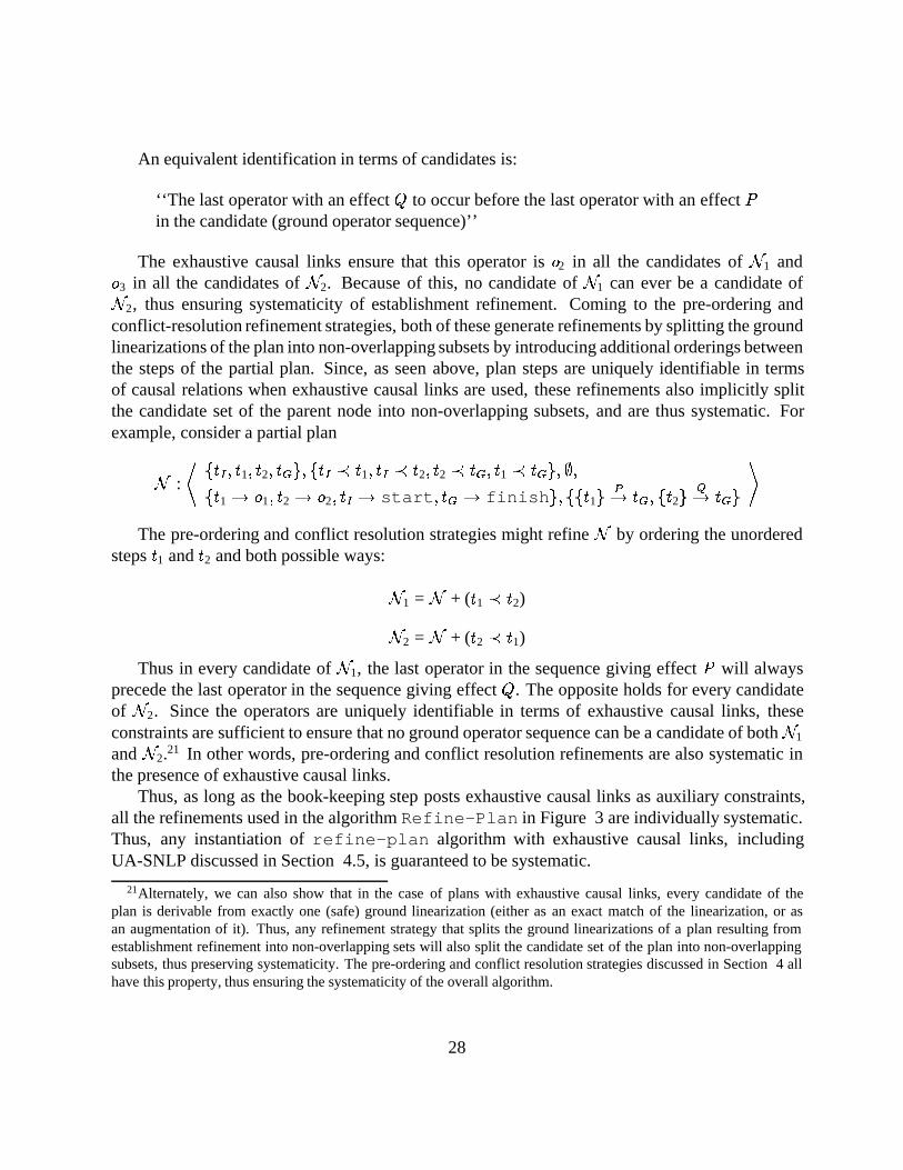
An equivalent identification in terms of candidates is:

‘‘The last operator with an effect Q to occur before the last operator with an effect Pin the candidate (ground operator sequence)’’

The exhaustive causal links ensure that this operator is o2 in all the candidates of N1 ando3 in all the candidates of N2. Because of this, no candidate of N1 can ever be a candidate ofN2, thus ensuring systematicity of establishment refinement. Coming to the pre-ordering andconflict-resolution refinement strategies, both of these generate refinements by splitting the groundlinearizations of the plan into non-overlapping subsets by introducing additional orderings betweenthe steps of the partial plan. Since, as seen above, plan steps are uniquely identifiable in termsof causal relations when exhaustive causal links are used, these refinements also implicitly splitthe candidate set of the parent node into non-overlapping subsets, and are thus systematic. Forexample, consider a partial plan

N :

*ftI ; t1; t2; tGg; ftI � t1; tI � t2; t2 � tG; t1 � tGg; ;;


Q! tGg

+

The pre-ordering and conflict resolution strategies might refine N by ordering the unorderedsteps t1 and t2 and both possible ways:

N1 = N + (t1 � t2)

N2 = N + (t2 � t1)

Thus in every candidate of N1, the last operator in the sequence giving effect P will alwaysprecede the last operator in the sequence giving effect Q. The opposite holds for every candidateof N2. Since the operators are uniquely identifiable in terms of exhaustive causal links, theseconstraints are sufficient to ensure that no ground operator sequence can be a candidate of bothN1

and N2.21 In other words, pre-ordering and conflict resolution refinements are also systematic inthe presence of exhaustive causal links.

Thus, as long as the book-keeping step posts exhaustive causal links as auxiliary constraints,all the refinements used in the algorithm Refine-Plan in Figure 3 are individually systematic.Thus, any instantiation of refine-plan algorithm with exhaustive causal links, includingUA-SNLP discussed in Section 4.5, is guaranteed to be systematic.

21Alternately, we can also show that in the case of plans with exhaustive causal links, every candidate of theplan is derivable from exactly one (safe) ground linearization (either as an exact match of the linearization, or asan augmentation of it). Thus, any refinement strategy that splits the ground linearizations of a plan resulting fromestablishment refinement into non-overlapping sets will also split the candidate set of the plan into non-overlappingsubsets, thus preserving systematicity. The pre-ordering and conflict resolution strategies discussed in Section 4 allhave this property, thus ensuring the systematicity of the overall algorithm.

28

Systematicity and overlapping linearizations: In the past, there has been a tendency to identifythe redundancy in the search space with overlapping linearizations of partial plans in the searchspace (e.g. [15, 7, 4]). From the formulation in this section, we note that systematicity implies onlythat no two partial plans in different branches of the search can share a safe ground linearization.Sharing of unsafe ground linearizations doesn’t affect systematicity since candidate set of a partialplan is related only to the safe ground linearizations (see Section 3.1). In particular, it is easy to seethat no augmentation of an operator sequence matching an unsafe ground linearization will ever bea candidate for a partial plan with auxiliary constraints specified by exhaustive causal links. Theproposition below thus follows:

Proposition 5 Systematicity implies non-overlapping ground linearizations only when all theplans in the search space are safe (i.e., all their ground linearizations are safe).

As remarked in Section 4.3.2, planners that do full conflict resolution (i.e., resolve all conflictsto auxiliary constraints before the next establishment cycle), maintain safe partial plans in theirsearch space. If such planners are systematic, then no two plans in different branches in theirsearch space will have overlapping ground linearizations.

Conflicting interpretations of Systematicity: There have been several conflicting interpretationsof ‘‘systematicity’’ of partial-order planning in the literature. Some researchers (c.f. [3]) haveinterpreted McAllester’s systematicity claim to mean that even though the same operator sequencemay appear in more than one branch, it will never have the same causal structure. This notionof causal structure systematicity is considerably weaker than the notion of systematicity whichwe defined above, and which is guaranteed by SNLP. Systematicity is stated in terms of operatorsequences rather than in terms of step names and causal structures. This is reasonable because stepnames and causal links are artifacts of the particular planning strategy, while systematicity shouldbe defined with respect to the space of potential candidates.

5.2.2 Strong Systematicity

Given a systematic refinement planner we have:

j}j =j=j

�

Thus, to bound search space size by the size of candidate space, we only need to bound theaverage size of the candidate set of the fringe nodes, �. This however turns out to be tricky. Inparticular, it is possible for the nodes in the termination fringe to have an empty candidate set (i.e.,there is no ground operator sequence satisfying the constraints of the partial plan corresponding tothat search node). The presence of such nodes can drive down the average size of the candidatesets �, and thus increase the size of the search space (we shall see an example of this in Figure 6).One way to guarantee that � � 1 would be to ensure that there are no inconsistent nodes in thesearch space with empty candidate sets. This leads us to the notion of strong systematicity.

29

Definition 14 (Strong Systematicity) A refinement search is said to be strongly systematic, ifand only if it is systematic and every node in the search tree is consistent.

From the definition of strong systematicity, we have � � 1 and thus j}j � j=j.

Proposition 6 The size of the termination fringe of a search tree generated by a strongly systematicrefinement search is strictly bounded by the size of the candidate space (i.e. j=j).

To convert a systematic search into a strongly systematic one, we only need to ensure thatevery node in the search space is consistent. Thus strong systematicity is guaranteed as long asthe consistency check is strong enough to prune all inconsistent partial plans generated by theplan refinements. Here, once again, we see a tradeoff between search space size and cost ofrefinement: As we discussed in Section 4.3, checking consistency of general partial orderingsagainst a set of exhaustive causal links is NP-hard [25]. The alternative of using pre-ordering orconflict resolution strategies to make consistency check tractable involves considerable amount ofadditional refinement over and above that required for establishment, and thus reduces �, there byincreasing the search space size.

It is interesting to note that pre-ordering and conflict resolution strategies provide strongsystematicity by ensuring that each partial plan in the search queue is safe. Strong systematicity,on the other hand, only requires consistency rather than safety. In Section 5.3, we will look at thepossibility of delaying or ignoring resolution of some conflicts (there by reducing the search spacesize), while still preserving strong systematicity.

5.2.3 On the Utility of Systematicity

Having spent considerable effort in clarifying the nature of systematicity in refinement planning,we shall now explore the practical utility of systematicity. As our discussion in Section 4.2demonstrated, systematicity is a natural culmination of efforts to reduce looping, redundancy andnon-minimal solutions in search space of refinement planners. The fact that contributor protection,which in some sense is a natural extension of protection intervals, and goal protection, can provablyeliminate redundancy from search space is quite pleasing.

In terms of the overall search space size, book keeping strategies, including those guaranteeingsystematicity, essentially allow planner to stop refining a partial plan earlier than would be thecase without book keeping (by adding auxiliary constraints to make the plan inconsistent). Thistends to increase � and thereby reduce the search space size. At the same time, if consistencycheck is done via conflict resolution/pre-ordering to ensure tractability, then this introduces morerefinement than would be done by a planner without any book-keeping strategy, and thus tends toreduce � and increase search space size. (Note that the increase in the search space size in thelatter case is not caused by systematicity, but rather by the way in which consistency check isimplemented)

30

Even if the search space size is smaller with systematicity, the performance of a planner doesnot depend solely on the worst case search space size. Like other forms of systematic search(c.f [11]), systematicity (or elimination of redundancy) in refinement planning is achieved atthe expense of increased commitment -- in this case to particular establishment structures (orcontributors). The elimination of redundancy afforded by systematicity (strong systematicity, tobe precise) can be very helpful when the solution density is very low, as it prevents the plannerfrom considering the same failing candidates more than once. However, when the solution densityis not particularly low, redundancy in the search space is only one of the many factors affectingthe performance of a refinement planner. Another (perhaps equally) important factor, in suchsituations, is the level of commitment in the planner. The use of protection intervals and causallinks, while reducing redundancy, also result in increased commitment to particular establishmentstructures. Increased commitment leads to higher backtracking, which in turn can adversely affectthe performance. This is in contrast to planners such as TWEAK, which avoid all forms of goalprotection and contributor protection, but at the expense of increased redundancy.

In Section 4.2, we emphasized that systematicity should not be seen in isolation, but ratheras part of a spectrum of methods for reducing redundancy in the search space. Our discussionin 4.2 suggests that every thing else (e.g., pre-ordering, conflict-resolution, termination and goalselection strategies) being equal, a planner that uses book-keeping based on exhaustive causallinks (like SNLP), and a planner that ignores book-keeping (like TWEAK), are in some senseat the extremes of the spectrum of approaches to redundancy-commitment tradeoff in refinementplanning. In [6, 7], we provided empirical support to the hypothesis that better approaches tothis tradeoff may lie in the middle of these two extremes. In particular, we showed that plannersusing multi-contributor causal structures may out-perform both TWEAK and SNLP under certaincircumstances. The latter maintain causal links, but do allow change of causal contributor duringplanning.

On a related note, the discussion in this paper also sheds some light on several extantmisconceptions about the role and utility of systematicity property.22 Since McAllester’s SNLPwas the first planner to state and claim this property, there has been a general tendency to attributeany and every perceived disadvantage of SNLP algorithm to its systematicity. For example, ithas been claimed ( e.g. [10]) that use of causal links and systematicity increases the effectivedepth of the solution both because it works on +ve as well as -ve threats, and because it forces theplanner to work on each precondition of the plan individually. Viewing SNLP as an instantiation ofRefine-Plan template, we see that it corresponds to several relatively independent instantiationdecisions, only one of which, viz., the use of exhaustive causal links in the book-keeping step, has adirect bearing on the systematicity of the algorithm. As we discussed above, and in Section 4.3, theuse of exhaustive causal links does not, ipso facto, increase the solution depth in any way. Rather,the increase in solution depth is an artifact of the particular solution constructor function, andconflict resolution and/or preordering strategies used in order to get by with tractable termination

22We have already addressed the misconceptions about the definition of systematicity property in the previoussections.

31

and consistency checks. As mentioned in Section 4.4, it is in principle possible to design aninstantiation of Refine-Plan which only uses an establishment based refinement, coupled witha more flexible, if costlier, solution constructor function (such as MTC-based constructor). Such aplanner clearly does not affect the solution depth -- both because it does not force the planner towork on each individual precondition separately, and because without conflict resolution, there isno notion of +ve (or -ve) threat resolution.

5.3 Reducing Search Space size by deferring conflicts

We have noted earlier (Section 4.3.2) that conflict resolution provides polynomial consistencycheck by further refining the refinements generated by the establishment step. From Equation2, we can see that every time we split a search node, we reduce � and thus increase the searchspace size. Furthermore, many of the conflicts in planning are ephemeral, in that in the course ofother goal establishments, they may naturally disappear. Thus, resolving conflicts as soon as theyappear may split the candidate set of a search node more than necessary, thereby reducing � andincreasing the search space size (see equation 2). This motivates the idea of deferring resolutionof some conflicts. In this section, we shall evaluate a variety of ideas for conflict deferment interms of our model of refinement planning.

To begin with, it is worth reiterating the fact that the strategies used to implement conflictresolution deferment and consistency check have no effect on the systematicity. Systematicityis a property of candidate sets, and as soon as the appropriate auxiliary constraint is added to apartial plan, its candidate set is determined. Further refinements of that partial plan by pre-orderingand conflict-resolution strategies, will not introduce any redundancy as long as they partition thecandidate sets; as discussed in Section 5.2.1). More practically, since solution-constructor functionwill only check for solution candidate within the candidate set of the given plan, the planner willnever return the same solution more than once.23

Strong systematicity, however, is a different matter. In general, arbitrary conflict defermentwill preserve strong systematicity only when the consistency check employed by the planner iscomplete. As mentioned in Section 4.3, a complete consistency check is exponential in most cases.Many implemented planners, such as SNLP, UCPOP and PEDESTAL, use polynomial consistencycheck that is only complete in the presence of undeferred conflict resolution. Specifically, a partialplan may be inconsistent as a whole (i.e., has empty candidate set), but the deferment of conflictresolution makes polynomial consistency check miss this inconsistency (as it may not yet havetranslated into order/binding inconsistency). While the inconsistency will be detected ultimately,arbitrary amount of refinement work may be done on inconsistent nodes in the mean time; thusdestroying strong systematicity. This point is illustrated in a telling fashion by the examplein Figure 6, which compares complete search space generated by systematic SNLP with thatgenerated by a variant called SNLP0 that postpones +ve threats, for the same planning problem.

23Although Harvey et. al. also make this point [4], our formulation of systematicity in Section 5.2.1 makes it selfevident.

32

Figure 6: Example demonstrating that arbitrary threat deferment does not ensure minimal worstcase search space size

The planner on the left is strongly systematic, while the one on the later is systematic but notstrongly systematic. Clearly, SNLP0 has a larger search space than that of SNLP. More over, theadditional nodes are all those with empty candidate sets (and will be pruned ultimately when theplanner attempts to resolve the +ve threats). This also points out that all else being equal a plannerwhich is merely systematic (and not strongly systematic) may have a larger search space than acorresponding planner that is not systematic. For example, it is easy to show that a planner whichcompletely ignores +ve threats (such as Pedestal [12]), is un-systematic (i.e., contains overlappingcandidate sets). However, it would stop before resolving the positive threats, and thus wouldgenerate a smaller search space than SNLP0. (Notice also that the search space of SNLP0 containspartial plans with overlapping linearizations. As remarked earlier, this does affect systematicity,since all the overlapping linearizations correspond to unsafe ground linearizations.)

In general, the only form of conflicts that can be deferred without affecting strong systematicityare those which can be provably resolved independently of how other conflicts are resolved (thisensures that consistency is not affected bya the deferment). However, it is often intractable to checkdynamically whether an conflict is of this type; thus increasing the refinement cost. Smith and Peot[25] propose an attractive alternative that relies on a tractable pre-processing step to recognizesome of the conflicts that are provably resolvable. Our discussion above shows that deferringconflicts based on such an analysis clearly preserves strong systematicity. In the following we willlook at some static threat deferment strategies.

33

5.3.1 Static conflict deferment strategies

Our discussions on search space size have until now concentrated on propositional planning withTWEAK representation. When we go to non-propositional planning, an important question is

regarding the definition of conflicts. Suppose we have a causal link fn0gP (x;y)! n and a step s

which can come between n0 and n and which has a delete literal P (u; v). The question is whetheror not s should be treated as a conflict (threat) by SNLP. McAllester [14] avoids this problem byusing an independent lifting transformation -- the question of whether P (x; y) is equal to P (u; v)is left to the lifting transformer, which will nondeterministically return either ‘‘yes’’ with bindingconstraints [x � u; y � v] or ‘‘no’’ with one of the bindings [x 6� u; y � v], [x 6� u; y 6� v] and[x � u; y 6� v]. The planner simply adds these constraints to the binding constraints of the plan,and does conflict resolution (i.e., add either promotion or demotion) if the answer was yes; orignores the conflict if the answer is no. If the added binding constraints are inconsistent with theexisting binding constraints in the plan, the plan eventually gets pruned by consistency checkingroutines.24

We can in fact improve the search space size by avoiding calling the lifting transformer alltogether. We can say that s is a threat if and only if it can fall between n0 and n and P (u; v)necessarily codesignates with P (x; y) modulo the binding constraints on the plan. Since mostconflicts of this type of are ephemeral, which will disappear when the variables concerned getbound to constants in the process of establishing various goals, the strategy of ignoring a conflictuntil it is necessarily codesignating, avoids splitting the search nodes unnecessarily and thusincreases �, (thereby reducing the size of the search space). Furthermore, as long as all variablesoccurring in the effects of an operator also occur in at least one of the preconditions (as is the casein most planning domains), and the initial state of the problem is completely ground, by the timeall establishments are completed, every possible conflict involving a variable will either becomea necessary conflict or a necessary non-conflict. Thus, there will never be a situation when therefinement cycle ends before resolving all conflicts.

Unfortunately however, this idea also can increase refinement cost for action representationsmore expressive than that of TWEAK. In particular, if we have variables with finite domains,checking whether the effects of a threat necessarily codesignate with a supported condition isNP-hard, thus making conflict detection itself intractable.

Further, deferring threats in this fashion does not in general preserve strong systematicity. Ifthe variables have finite domains, it is possible that a set of conflicts are all individually separable,but all of them are not separable together. As an example, consider a partial plan with two conflicts:

24It is interesting to note that the lifting idea introduced in McAllester’s paper, is not used in other implementationsof SNLP. The most popular implementation of SNLP, done by Barrett and Weld, (hence forth referred to as UW-SNLP)

defines s to be a threat to link fn0gP (x;y)! n as long as P (u; v) can possibly unify fsg

p! w, if v has an add or delete

literal q such that q can possibly unify with p modulo the bindings on the current plan. To resolve a threat, UW-SNLPeither (a) adds the binding [x � u; y � v] and promotes or demotes s or (b) orders s to come necessarily between n0

and n (this avoids redundancy with respect to promotion and demotion strategies) makes one partial plan for each ofthe non-overlapping binding sets [x 6� u; y � v], [x 6� u; y 6� v] and [x � u; y � v].

34

ft1gP (A)! t2 t3 and ft01g

Q(B)! t02 t3, where t3 has two delete list literals P (x) and Q(x), and x

has the domain fA;Bg. Here, both conflicts are individually separable, but in conjunction, theyare unseparable. The only general way to guarantee strong systematicity in such cases is to checkif the conflicts are resolvable together. The latter makes the deferment check intractable. Thistype of scenario does not occur for TWEAK representation which assumes variables with infinitedomains, because for infinite domain variables, a set of non-codesignation constraints will neverentail a codesignation constraint.

(In [22] Peot and Smith describe a planner called DSep which is a variant of SNLP that defersthreats until they are ‘‘unseparable’’, i.e., necessarily codesignating, and provide a proof that DSepsearch space is no larger than that of SNLP which folds conflict resolution into establishment. Ourdiscussion above shows that their proof holds only for the case of variables with infinite domains.For variables with finite domains, DSep will allow inconsistent nodes into its search space as wellas refine them. SNLP which folds conflict resolution into establishment would have pruned suchplans early on. Thus, it is possible for DSep to have a larger search space.)

5.4 Effect of Termination and Pruning Checks on Search Space Size

The solution constructor function, sol, used by the planner can also have an effect on the searchspace size of the refinement planner: The earlier in search we are able to pick a solution candidate,the larger the value of �. In the case of planning, a planner that uses a termination check based on anecessary and sufficient truth criterion will be able to terminate before explicitly establishing eachopen condition, than one which uses a protection interval/causal link based termination condition,requiring the planner to explicitly work on each of the goals. Thus, the former has a larger valueof � (and thus smaller search space) than the latter, all else being equal. Once again, the flip side isthat for general partial order planners with expressive action representations, checking necessarytruth of a condition is intractable.

Another way the sol function can reduce the search space size is by pruning unpromisingnodes earlier. Recall that sol function prunes a partial plan, when it can guarantee that there is nosolution candidate in the candidate set of that node. By pruning such nodes as early as possible,the planner can increase the size of candidate sets of the failing nodes in the termination fringe,there by increasing � and reducing the size of the search space. Pruning involves computing macrocharacteristics of the candidate set of the node, analyzing it with respect to the outstanding goals,and showing that it does not contain a solution candidate with respect to them. This latter is bestseen as a look-ahead computation. Few classical refinement planners employ this type of pruning.An example is the FORBIN planner [2], which does a significant amount of look-ahead schedulingbefore allowing a partial plan to enter the search queue and expanded. Once again, there is atradeoff between the cost of the pruning strategy and the extent to which it can reduce the searchspace size [8].

35

5.5 Effect of pre-ordering and Conflict Resolution Strategies under Depth-firstregimes

In the previous sections, we noted that pre-ordering and conflict resolution strategies, while provid-ing tractable consistency check, also further refine the refinements provided by the establishmentstep. They thus increase the search space size by reducing �. While this would imply thatpre-ordering and conflict resolution strategies would explore more nodes in breadth-first searchregimes, it does not predict the size of the search space explored under depth-first search regimes.In this section, we will use our model of refinement planning to analyze these strategies underdepth-first regime. To simplify the analysis, we will consider four planners that use contributorprotection and guarantee strong systematicity: SNLP which uses conflict resolution to ensuretractable refinement; SNLP*, which is like SNLP, but uses a non-polynomial consistency checkinstead of conflict resolution; UA-SNLP which uses pre-ordering to ensure tractable refinement;and finally, TOCL which uses total ordering.

Since pre-ordering and conflict resolution split a search node into multiple search nodes, it isclear that the value of � is largest in SNLP*, and correspondingly smaller in SNLP, UA-SNLP,and TOCL. Thus, the search space sizes of the planners increase in the order SNLP* � SNLP �UA-SNLP � TOCL.

To estimate the size of the search space explored under depth-first regimes, we need to estimatethe probability of making successful choice. Suppose we assume that all the planners pick thenext node to be refined randomly from the set of refinements that they generated. In terms ofcost of depth-first search, the critical question is ‘‘what is the probability that each planner picks arefinement that contains at least one solution candidate.’’ We shall use the somewhat inaccurateterm ‘‘success probability’’ to refer to this probability. Even small changes in this probability canhave dramatic effects on performance since picking a wrong refinement at the very beginning ofsearch can have very high impact on the performance of depth-first search.

Consider a search node N that SNLP* picked up for refinement. Suppose the averagebranching factor of SNLP’s refinement strategy is b. SNLP will thus refine N into a set of bchildren nodes fN1;N2; � � � ;Nbg. Since SNLP* is systematic, the candidate sets of these nodesdefine a partitioning of the candidate set of N . Under depth first strategy, SNLP* will then pickone of the nodes, Ni, for refinement.

Since SNLP, UA-SNLP and TOCL differ from SNLP* only in terms of additional refinementsthey employ (to provide tractable consistency check), we can look at their operation as furtherrefining each Ni into some partition of its candidate set fN 1

i ;N2i ; � � � ;N

mi g (as dictated by the

pre-ordering/conflict resolution strategy), and selecting the next node to be refineed from this set.It is clear that the success probability of SNLP, UA-SNLP and TOCL are connected to the

success probability of SNLP* (since after all they are taking the refinements of SNLP and splittingthem further). Suppose Ni contains mi solution candidates. As long as pre-ordering partitionsNi into mi or less refinements such that each refinement has a solution candidate, the successprobability will tend to increase or remain the same. If on the other hand, Ni is split into more

36

than mi refinements, then the success probability will tend to decrease. (this means that anypre-ordering choice which splits nodes containing no solution candidates will tend to reduce thesuccess probability). Even whenNi is split into less than mi refinements, if the solution candidatesare non-uniformly distributed such that not all refinements have solution candidates in them, thenonce again, the success probability will tend to decrease.

The above discussion shows that only when the pre-ordering/conflict resolution strategy isclairvoyant enough to split each Ni based on the number of solution candidates in the node, is itlikely to increase the success probability. The pre-ordering/conflict resolution strategies used bySNLP, UA-SNLP and TOCL, use the constraints on the current partial plan, rather than knowledgeabout the number of solution candidates in a given node. Thus, they split the nodes in a somewhatuniform fashion that is oblivious to the number of solution candidates in the node. Thus, unlessthe domain is such that the syntactic splitting done by the pre-ordering strategies will have highcorrelation with the number of solution candidates in each node, there is no reason to expect thatSNLP, UA-SNLP and TOCL will preserve or increase the success probability compared to SNLP*.

If we approximate the behavior of all the refinement strategies as a random partitioning ofcandidate set ofN into some number of children nodes, then it is possible to provide a quantitativeestimate of the success probabilities of all the three planners. To do this, let us assume as beforethat b is the average number of children nodes generated by the refinement strategy of SNLP*. Letus assume that to begin with N has m solution candidates in its candidate set. SNLP* partitionsthe candidate set of SNLP into b new refinements. The success probability of SNLP* is justthe probability that a random node picked from these b new nodes contains at least one solutioncandidate. This is just equal to q(m; b) where q(m;n) is the binomial distribution:25

q(m;n) =m�1Xi=0

m

n

!1

nm�i

�1�

1n

�i

Now suppose that the average splitting factor of SNLP is ss (i.e., SNLP splits each SNLP*node into su new nodes). This means that SNLP splitsN into b� ss nodes. The success probabilityof SNLP is thus q(m; b� ss). Similarly, if we assume that su and st as the splitting factors forUA-SNLP and TOCL respectively, then their success probabilities are q(m; b� su), q(m; b� st)respectively. Since TOCL’s preordering strategy is more eager than that of UA-SNLP, whileUA-SNLP orders steps based on effects and preconditions, without regard to the causal links, weexpect ss � su � st.

It can be easily verified that for fixed m, q(m;n) monotonically decreases with increasing n.Thus

q(m; b) � q(m; b� ss) � q(m; b� su) � q(m; b� st)

That is, under the random partitioning assumptions, the four planners, in the increasing orderof success probability are: SNLP* � SNLP � UA-SNLP � TOCL. (Although lower success

25q(m;n) is the probability that a randomly chosen urn will contain at least one ball, whenm balls are independentlyrandomly distributed into n urns. This is equal to probability that a randomly chosen urn will have all m balls plus theprobability that it will have m � 1 balls and so on plus the probability that it will have 1 ball.

37

probability will suggest higher search space size, in terms of performance, the performance penaltyof the larger search space size may still be offset by the reduced per-node refinement cost.)

6 Concluding Remarks

Much of the formalization work in classical planning concentrated on soundness and completenessof the planning algorithms. Very little comparative analysis has been done on the search spacecharacteristics of the multitude of existing planning algorithms. We believe that the large part ofthe reason for this lack was the seemingly different vocabularies/frameworks within which manyof the algorithms have been expressed.

In this paper, we have shown that if we take the view of planning as refinement searchseriously, then we can indeed provide a generic refinement planning algorithm such that thefull variety of classical planning algorithms can be expressed as specific instantiations of thisalgorithm. We have used our generic refinement planning algorithm to provide a coherent rationalreconstruction of main ideas of classical planning algorithms. We have shown that this typeof unified approach facilitates separating important ideas from ‘‘brand names’’ of the planningalgorithms with which they have been associated in the past. The usual differentiations betweenplanning algorithms such as ‘‘total order vs. partial order’’, ‘‘systematic vs. non-systematic’’,‘‘causal link based vs. non-causal link based’’, ‘‘truth criterion based vs. secondary preconditionbased’’, and ‘‘TWEAK representation vs. ADL representation’’ have are all properly groundedwithin this unified refinement search framework. In many cases, the differences are shown to bea spectrum rather than dichotomy. All this, in turn facilitates a fruitful integration of competingapproaches. We demonstrated this by providing a hybrid planning algorithm called UA-SNLP thatborrows ideas from two seemingly different planning algorithms.

Our model of refinement planning clarifies the nature and utility of several oft-misunderstoodideas for bounding search space size, such as goal protection, protection intervals, and systematicity.We provided a clear formulation of the notion of systematicity and clarified several misconceptionsabout this property. Our model also provides a basis for analyzing a variety of ideas for improvingplanning performance, such as conflict deferment, deliberative goal selection strategies, leastcommitment, polynomial time consistency checks, etc., in terms of the tradeoffs between searchspace size and refinement cost that they offer. Because of our unified treatment, we were ableto evaluate the utility of particular approaches not only for propositional STRIPS and TWEAKrepresentations, but also under more expressive representations such as ADL. Our comparativeanalysis of the utility of pre-ordering and and conflict resolution techniques on the successprobability of the planner show that the unified model also provides leverage in estimatingexplored search space in depth first regimes.

Our work also has important implications to the research on comparative analyses of partialorder planning techniques. In the past, such comparative analyses tended to focus on a wholistic‘‘black-box’’ view brand-name planning algorithms, such as TWEAK and SNLP (c.f. [10]). We

38

believe that it is hard to draw meaningful conclusions from such comparisons since when seen asinstantiations of our Refine-Plan algorithm, they differ in a variety of dimensions (see Table1). A more meaningful approach, facilitated by the unified framework of this paper, involvescomparing instantiations of Refine-Plan that only differ in a single dimension. For example, ifour objective is to judge the utility of specific protection (book-keeping) strategies, we could keepeverything else constant and vary only the book keeping step in Refine-Plan. In contrast, whenwe compare TWEAK with SNLP, we are not only varying the protection strategies, but also the goalselection, conflict resolution and termination (solution constructor) strategies, making it difficultto form meaningful hypotheses from empirical results. After all, the fact that SNLP algorithmuses a protection-based termination check, and an arbitrary goal selection method, also does notmean that any instantiation of Refine-Plan that uses exhaustive causal links must use the sametermination and goal-selection checks. In particular, it is perfectly feasible to construct a planningalgorithm which uses MTC-based goal-selection and termination constraints like TWEAK, butemploys exhaustive causal links (like SNLP). A comparison between this algorithm and TWEAKwill clearly shed more light on the effect of exhaustive causal links and systematicity on planningperformance. Similar experimental designs can be made for comparing the utility of pre-orderingstrategies, conflict resolution strategies, termination criteria and goal selection criteria, based onthe Refine-Plan algorithm template.

While refinement search provides a unified framework for many classical planning algorithms,it is by no means the sole model of planning in town. The so called transformational approachesto planning [13] provide an important alternative approach. The latter may be better equipped tomodel the HTN planners such as SIPE, NONLIN and OPLAN, which view planning as the processof putting together relatively stable canned plan fragments, and teasing out interactions betweenthem, rather than as a process of starting with null plan and adding constraints.26 On a related note,our current framework does not adequately account for the so-called state-based planners. We arecurrently working towards rectifying this situation.

The most significant contribution of our paper is that it provides a framework for foregroundingand analyzing a variety of tradeoffs within a single coherent refinement search framework. Whileour analysis has been qualitative in many places, we believe that this work provides the basis forfurther quantitative/empirical analysis of several tradeoffs. Exploration of these tradeoffs providesan important avenue for future research.

Acknowledgements

I benefited greatly from the (e-mail) discussions with David McAllester on the nature of generalrefinement search. Discussions with Bulusu Gopi Kumar helped significantly in clarifying mythinking on a variety of issues; most notably on the material in Section 5.5. Thanks are also due to

26Similar views are expressed by McDermott. In [13], he suggests that the plan-fragments used by hierarchicalplanners ought to be written in such a way that even with no further planning at all they can be conjoined with otherplans (although the result may be suboptimal). The purpose of planning is then to remove the resulting inefficiencies.

39

Mark Drummond, Will Harvey, Laurie Ihrig, Suresh Katukam, Richard Korf, Pat Langley, SteveMinton, Ed Pednault, Mark Peot, Dave Smith, Austin Tate and Dan Weld for helpful commentsduring the course of this research.

References

[1] D. Chapman. Planning for conjunctive goals. Artificial Intelligence, 32:333--377, 1987.

[2] T. Dean, R.J. Firby, and D. Miller. Hierarchical planning involving deadlines, travel timeand resources Computational Intelligence, Vol. 4, 381-398 (1988).

[3] S. Hanks and D. Weld. Systematic Adaptation for Case-Based Planning. In Proc. 1st Intl.Conf. on AI Planning Systems, 1992.

[4] W.D. Harvey and M.L. Ginsberg and D.E. Smith. Deferring Conflict Resolution RetainsSystematicity. Submitted to AAAI-93.

[5] J. Jaffar and J. L. Lassez. Constraint logic programming. In Proceedings of POPL-87, pages111--119, 1987.

[6] S. Kambhampati. Multi-Contributor Causal Structures for Planning: A Formalization andEvaluation. Arizona State University Technical Report, CS TR-92-019, July 1992. (Toappear in Artificial Intelligence. A preliminary version appears in the Proc. of First Intl. Conf.on AI Planning Systems, 1992).

[7] S. Kambhampati. On the Utility of Systematicity: Understanding tradeoffs between redun-dancy and commitment in partial order planning In Proceedings of IJCAI-93, Chambery,France, 1993.

[8] S. Kambhampati and E. Cohen. On the utility of minimality-based pruning algorithms inpartial order planning. ASU CSE Technical Report (In Preparation).

[9] S. Kambhampati and D.S. Nau. On the Nature and Role of Modal Truth Criteria in PlanningTech. Report. ISR-TR-93-30, Inst. for Systems Research, University of Maryland, March,1993.

[10] C. Knoblock and Q. Yang. A Comparison of the SNLP and TWEAK planning algorithms. InProc. of AAAI Spring Symp. on Foundations of Automatic Planning: The Classical Approachand Beyond. March, 1993.

[11] P. Langley. Systematic and Nonsystematic search strategies. In Proc. 1st Intl. Conferenceon AI Planning Systems, June 1992.

[12] D. McDermott. Regression Planning. Intl. Jour. Intelligent Systems, 6:357-416, 1991.

40

[13] D. McDermott. Transformational planning of reactive behavior. Yale University TR CSDRR-941, December, 1992.

[14] D. McAllester and D. Rosenblitt. Systematic Nonlinear Planning. In Proc. 9th AAAI, 1991.

[15] S. Minton, J. Bresina and M. Drummond. Commitment Strategies in Planning: A ComparativeAnalysis. In Proc. 12th IJCAI, 1991.

[16] S. Minton, M. Drummond, J. Bresina and A. Philips. Total Order vs. Partial Order Planning:Factors Influencing Performance In Proc. KR-92, 1992.

[17] D.S. Nau, V. Kumar and L. Kanal. General Branch and Bound, and its relation to A� andAO� Artificial Intelligence, Vol. 23, 1984, pp. 29-58.

[18] N.J. Nilsson. Principles of Artificial Intelligence. Tioga Publishers, Palo Alto, CA, 1980.

[19] J. Pearl. Heuristics: Intelligent Search Strategies for Computer Problem Solving. Addison-Wesley, Reading, Massachusettes (1984).

[20] E.P.D. Pednault. Synthesizing Plans that contain actions with Context-Dependent EffectsComputational Intelligence, Vol. 4, 356-372 (1988).

[21] E.P.D. Pednault. Generalizing nonlinear planning to handle complex goals and actions withcontext dependent effects. In Proc. IJCAI-91.

[22] M.A. Peot and D.E. Smith. Threat-Removal Strategies for Nonlinear Planning. In Proc.AAAI-93

[23] J.S. Penberthy and D. Weld. UCPOP: A Sound, Complete, Partial Order Planner for ADL.In Proc. KR-92, November 1992.

[24] A. Barrett and D. Weld. Partial Order Planning: Evaluating Possible Efficiency GainsTechnical Report 92-05-01, Department of Computer Science and Engineering, Universityof Washington, Seattle, WA, June 1992.

[25] D.E. Smith and M.A. Peot. Postponing Simple Conflicts in Nonlinear Planning. In Workingnotes of AAAI Spring Symp. on Foundations of Automatic Planning: The classical approachand Beyond.

[26] G.J. Sussman. A Computer Model of Skill Acquisition. American Elsevier, New York, 1975

[27] A. Tate. Generating Project Networks. In Proceedings of IJCAI-77, pages 888--893, Boston,MA, 1977.

[28] Q. Yang, J. Tenenberg and S. Woods. Abstraction in nonlinear planning University ofWaterloo Technical Report CS-91-65, 1991.

41

Contents

1 Introduction 1

2 Goals, Solutions and Completeness in classical planning 2

3 Planning as Refinement Search 43.1 Semantics of Partial Plans : : : : : : : : : : : : : : : : : : : : : : : : : : : : : : : : : : 43.2 A generic algorithm template for refinement planning : : : : : : : : : : : : : : : : : : : : 8

4 A Rational Reconstruction of main ideas of Refinement Planning 114.1 Establishment : : : : : : : : : : : : : : : : : : : : : : : : : : : : : : : : : : : : : : : : 13

4.1.1 Goal Selection : : : : : : : : : : : : : : : : : : : : : : : : : : : : : : : : : : : : 144.2 Book Keeping and Posting of Auxiliary Constraints : : : : : : : : : : : : : : : : : : : : : 14

4.2.1 Motivation : : : : : : : : : : : : : : : : : : : : : : : : : : : : : : : : : : : : : : 144.2.2 Book-keeping through Goal Protection : : : : : : : : : : : : : : : : : : : : : : : 154.2.3 Goal Protection by Protection Intervals : : : : : : : : : : : : : : : : : : : : : : : 164.2.4 Redundancy elimination through Contributor Protection : : : : : : : : : : : : : : 17

4.3 Consistency Check, Pre-ordering and Conflict Resolution : : : : : : : : : : : : : : : : : : 184.3.1 Pre-ordering for tractable plan handling : : : : : : : : : : : : : : : : : : : : : : : 194.3.2 Conflict Resolution : : : : : : : : : : : : : : : : : : : : : : : : : : : : : : : : : 20

4.4 Solution Constructor function : : : : : : : : : : : : : : : : : : : : : : : : : : : : : : : : 214.5 Integrating Competing Approaches: Case study of UA-SNLP : : : : : : : : : : : : : : : : 22

5 Search Space size, refinement cost and Performance 245.1 A model for estimating search space size : : : : : : : : : : : : : : : : : : : : : : : : : : 245.2 Bounding Search Space with the size of the candidate Space: Systematicity and Strong

Systematicity : : : : : : : : : : : : : : : : : : : : : : : : : : : : : : : : : : : : : : : : : 265.2.1 Systematicity : : : : : : : : : : : : : : : : : : : : : : : : : : : : : : : : : : : : 265.2.2 Strong Systematicity : : : : : : : : : : : : : : : : : : : : : : : : : : : : : : : : : 295.2.3 On the Utility of Systematicity : : : : : : : : : : : : : : : : : : : : : : : : : : : : 30

5.3 Reducing Search Space size by deferring conflicts : : : : : : : : : : : : : : : : : : : : : : 325.3.1 Static conflict deferment strategies : : : : : : : : : : : : : : : : : : : : : : : : : 34

5.4 Effect of Termination and Pruning Checks on Search Space Size : : : : : : : : : : : : : : 355.5 Effect of pre-ordering and Conflict Resolution Strategies under Depth-first regimes : : : : : 36

6 Concluding Remarks 38

i

List of Figures

1 A generic Refinement search strategy : : : : : : : : : : : : : : : : : : : : : : : 92 A generic planning algorithm for refinement planning: Initial Call : : : : : : : : 113 A generic algorithms for refinement planning: Refinement Procedure : : : : : : : 124 Examples showing redundancy and looping in TWEAK search space. In all the

examples, the operators are shown with preconditions on the right side, and effectson the left (with ‘‘+’’ sign for add list literals, and ‘‘�’’ sign for delete list literals).The Init and Goal lists specify the problem. The example on left is adopted fromMinton et. al. : : : : : : : : : : : : : : : : : : : : : : : : : : : : : : : : : : : : 17

5 A non-minimal plan produced in spite of exhaustive causal links : : : : : : : : : 186 Example demonstrating that arbitrary threat deferment does not ensure minimal

worst case search space size : : : : : : : : : : : : : : : : : : : : : : : : : : : : 33

ii

planning as refinement search: a unified framework for

Documents