plant intelligence based metaheuristic optimization algorithms · 2017-11-01 · plant intelligence...

Artif Intell Rev (2017) 47:417–462DOI 10.1007/s10462-016-9486-6

Plant intelligence based metaheuristic optimizationalgorithms

Sinem Akyol1 · Bilal Alatas2

Published online: 30 May 2016© Springer Science+Business Media Dordrecht 2016

Abstract Classical optimization algorithms are insufficient in large scale combinatorialproblems and in nonlinear problems. Hence, metaheuristic optimization algorithms havebeen proposed. General purpose metaheuristic methods are evaluated in nine differentgroups: biology-based, physics-based, social-based, music-based, chemical-based, sport-based, mathematics-based, swarm-based, and hybrid methods which are combinations ofthese. Studies on plants in recent years have showed that plants exhibit intelligent behaviors.Accordingly, it is thought that plants have nervous system. In this work, all of the algorithmsand applications about plant intelligence have been firstly collected and searched. Informationis given about plant intelligence algorithms such as Flower Pollination Algorithm, InvasiveWeed Optimization, Paddy Field Algorithm, Root Mass Optimization Algorithm, ArtificialPlant Optimization Algorithm, Sapling Growing up Algorithm, Photosynthetic Algorithm,Plant Growth Optimization, Root Growth Algorithm, Strawberry Algorithm as Plant Prop-agation Algorithm, Runner Root Algorithm, Path Planning Algorithm, and Rooted TreeOptimization.

Keywords Plant intelligence · Global optimization · Metaheuristic methods

1 Introduction

Most of the optimization algorithms need mathematical models for system modelling andobjective function. Establishment of a mathematical model is mostly hard for complex sys-tems. Even though the model is established, it cannot be used due to high cost of solution

B Sinem [email protected]

Bilal [email protected]

1 Department of Computer Engineering, Tunceli University, Tunceli, Turkey

2 Department of Software Engineering, Firat University, Elazig, Turkey

123

http://crossmark.crossref.org/dialog/?doi=10.1007/s10462-016-9486-6&domain=pdf

418 S. Akyol, B. Alatas

time. Classical optimization algorithms are insufficient in large-scale combinational and non-linear problems. Such algorithms are not effective in adaptation a solution algorithm for agiven problem. In most cases, this requires some assumptions whose approval of validitycan be difficult. Generally, because of natural solution mechanism of classical algorithms,significant problem is modeled the way that algorithm can handle it. Solution strategy of clas-sical optimization algorithms generally depends on type of objective and constraints (linear,non-linear etc.) and depends on type of variables (integer, real) used in modelling of prob-lem. Furthermore, effectiveness of the classical algorithms highly depends on solution space(convex, non-convex etc.), the number of decision variable, and the number of constraints inproblem modelling.

Another important deficiency is that; if there are different types of decision variables,objectives, and constraints, general solution strategy is not presented for implemented prob-lem formulation. In other words, most of algorithms solve models which have certain type ofobject function or constraints. However, optimization problems in many different areas suchas management science, computer, and engineering require concurrently different types ofdecision variables, object function, and constraints in their formulation. Therefore, meta-heuristic optimization algorithms are proposed. These algorithms become quite popularmethods in recent years, due to their good computation power and easy conversion. Inother words, a metaheuristic program, written for a specific problem with a single objec-tive function, can be adapted easily to a multi objective version of this problem or a differentproblem.

Studies in recent years indicate that plants also exhibit intelligent behaviors. Accordingto this, it is thought that plants have nervous system. For example, in roots, imported lightand poison information are transmitted to growth center in root tips and the roots performorientation according to that. Additionally, it is thought that plants make contact with externalworld using electric current.An example for this is defensemechanismwhich is shownagainstto aphid or caterpillar by plants. After the first developed attack, plants produce secretionswhich can make worse taste or which can poison their enemy.

Inspiring by the flow pollination process of flowery plants, Flower Pollination Algorithm(FPA), has been developed in 2012 by Yang (2012). Invasive Weed Optimization (IWO),inspired from the phenomenon of colonization of invasiveweeds in nature, has been proposedby Mehrabian and Lucas (2006). It is based on ecology and weed biology. Paddy FieldAlgorithm (PFA), which simulates growth process of paddy fields, is another plant basedmetaheuristic algorithm and has been proposed by Premaratne et al. (2009). Root MassOptimization (RMO) is based on the process of root growth and has been proposed byQi et al. 2013. Artificial Plant Optimization Algorithm (APOA) simulates growth modelof plants which includes photosynthesis and phototropism mechanism (Zhao et al. 2011).Sapling Growing up Algorithm (SGuA) is a computational method based on cultivating,growing up, and mating of saplings and it is developed for efficient solutions to search andoptimization problems (Karci 2007a).

Photosynthetic Algorithm (PA) is based on the processes of Calvin–Benson cycle andphotorespiration cycle for the plants (Murase 2000). Plant Growth Optimization (PGO) isproposed to simulate plant growth with a realistic way considering the spatial occupancy,account branching, phototropism, and leaf growth. Themain purpose of the model is to selectactive point by comparing themorphogen concentration for increasing theL-system (Cai et al.2008). Root Growth Algorithm (RGA) is another plant based metaheuristic algorithm andsimulates root growth of plants based on L-system (Zhang et al. 2014).

Strawberry algorithm has been proposed as an exemplar of Plant Propagation Algorithm(PPA). It maps an optimization problem onto survival optimization problem of strawberry

123

Plant intelligence based metaheuristic optimization algorithms 419

plant and adopts strategy of survival in the environment for searching points in the searchspace which give the best values and ultimately the best value (Salhi and Fraga 2011). RunnerRoot Algorithm (RRA) is inspired by plants such as strawberry and spider plants which arespread through their runners and also which develop roots and root hairs for local searchfor minerals and water resources (Merrikh-Bayat 2015). Path Planning Algorithm is basedon plant growth mechanism (PGPP) which uses phototropism, negative geotropism, apicaldominance, and branching as basic rules (Zhou et al. 2016). One of themost recent plant basedalgorithm is Rooted Tree Optimization (RTO) and it is based on the intelligent behaviors ofroots which select their orientation according to the wetness (Labbi et al. 2016). Researchesabout new versions and applications of these algorithms incrementally continue.

In this work, in the second part, the information is given about metaheuristic optimizationand it is mentioned that why metaheuristic algorithms are needed. In the third part, plantintelligence is mentioned; optimization algorithms developed inspired by plant intelligenceare examined and related works with these algorithms are described. FPA, IWO, PFA, RMOAlgorithm, APOA, SGuA, PA, PGO, RGA, Strawberry Algorithm as PPA, RRA, PGPP,and RTO are explained. In the fourth part, discussions about general evaluations of thesealgorithms are presented and in the fifth part, the work is concluded along with future works.

2 Metaheuristic optimization

In most of the real life problems, solution space of the problem is infinite or it is too largefor assessment of all the solutions. Therefore, with evaluating solutions, a good solution isneeded to be found in acceptable time. Actually, for such problems, evaluating solutions inacceptable time has the samemeaningwith evaluating “some solutions” in the whole solutionspace. Selection of some solutions depending on what and how they are selected changesaccording to metaheuristic method. It cannot be guaranteed that optimal solution is includedin the solutions which get involved in the evaluation. Therefore, the solution, proposed bymetaheuristic methods for an optimization problem, must be perceived as a good solution,not as an optimal solution (Cura 2008).

They are criteria or computer methods identified in order to decide effective ones ofvarious alternative movements for achieving any purpose or the goal. Such algorithms haveconvergence property, but they cannot guarantee exact solution, they can only guarantee asolution which closes to exact solution.

The reasons of why metaheuristic algorithms are needed are as follows:

(a) Optimization problem can have a structure that the process of finding the exact solutioncannot be defined

(b) Metaheuristic algorithms can bemuch simpler from the point of decisionmaker, in termsof comprehensibility.

(c) Metaheuristic algorithms can be used as a part of process of finding the exact solution,and learning purpose.

(d) Generally, the most difficult parts of real world problems (which purposes and whichrestrictions must be used, which alternatives must be tested, how problems data must becollected) are neglected in the definitions made with mathematical formulas. Faultinessof the data used in process of determining model parameters can cause much largererrors than sub-optimal solution produced by metaheuristic approach (Karaboga 2011).

General purposed metaheuristic methods are evaluated in eight different groups whichare biology based, physic based, swarm based, social based, music based, chemistry based,

123


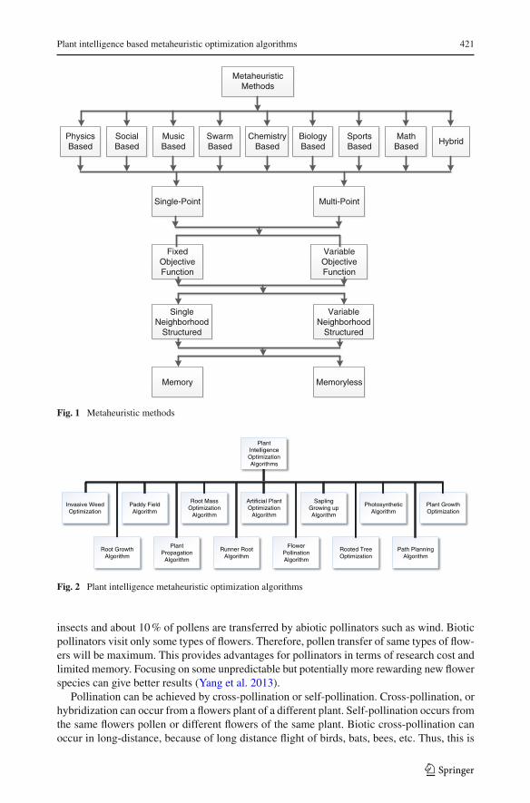
sport based, and math based. Furthermore, there are hybrid methods which are combina-tion of these. These mentioned methods are presented in Fig. 1. Genetic Algorithm (GA)(Holland 1975), differential evolution algorithm (Storn and Price 1995), and biogeography-based optimization (Simon 2008) are biology based; parliamentary optimization algorithm(Borji 2007), teaching-learning-based optimization (Ghasemi et al. 2015; Rao et al. 2011),and imperialist competitive algorithm (Atashpaz-Gargari and Lucas 2007a, b; Ghasemi et al.2014) are social based; artificial chemical reaction optimization algorithm (Alatas 2011a)and chemical reaction optimization (Lam and Li 2010) are chemistry based; harmony searchalgorithm (Geem et al. 2001) is music based; gravitational search algorithm (Rashedi et al.2009), intelligent water drops algorithm (Shah-Hosseini 2009), and charged system search(Kaveh and Talatahari 2010) are physics based; Particle Swarm Optimization (PSO) algo-rithm (Kennedy and Eberhart 1995), cat swarm optimization (Chu et al. 2006), ant colonyalgorithm (Dorigo et al. 1991), monarch butterfly optimization (Wang et al. 2015), groupsearch optimizer (He et al. 2006, 2009), and cuckoo search via Levy flights (Yang and Suash2009) are swarm based; league championship algorithm (Kashan 2009) is sport based; andbase optimization algorithm (Salem 2012), and Matheuristics (Maniezzo et al. 2009) aremath based algorithms and methods. Cultural algorithm (Jin and Reynolds 1999) and colo-nial competitive differential evolution (Ghasemi et al. 2016) can be classified as both biologybased and social based algorithm.

Although there are many successful search and optimization algorithms and techniquesin the literature; design, development, and implementation of new techniques is an importanttask under the philosophy of improvement in the scientific field and always searching todesign better. The best algorithm that gives the best results for all the problems has not yetbeen designed, that is why constantly new artificial intelligence optimization algorithms areproposed or some efficient additions or modifications have been performed to the existingalgorithms.

3 Plant intelligence optimization algorithms

As a result of previous studies, it is observed that plants have gender identity and immunesystem. Furthermore, recent studies show that plants exhibit intelligent behavior. Accordingto this, it is thought that plants have nervous system. For example, in roots, imported lightand poison data are transmitted to growth centers in root tips, and roots perform orientationaccording to this. As another consideration, plants are considered to be contacting with theexternal world by electric currents. Defense mechanism, which is shown against to aphid orcaterpillar by plants, can be shown as an example for this. After the first attack takes place,plants will worsen their taste or produce secretions which can poison their enemy.

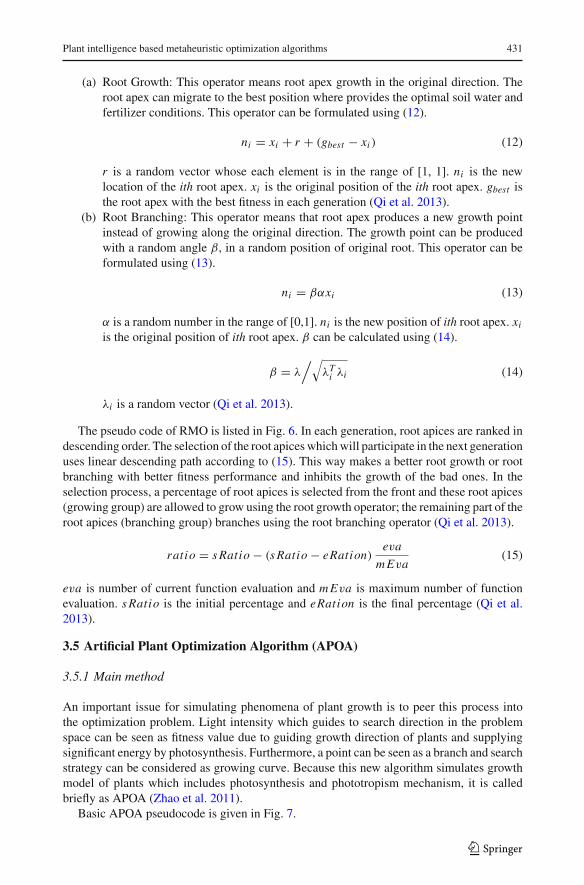
The metaheuristic optimization algorithms which are developed by inspiration from plantintelligence have been shown in Fig. 2 and explained in subsections.

3.1 Flower Pollination Algorithm (FPA)

3.1.1 Characteristic of flower pollination

It is estimated that, in nature, there are over a quarter of a million types of flowery plants.Approximately 80% of all plant species are flowery plant. Flowery plants have been evolv-ing for more than 125 million years. The main objective of a plant is reproducing throughpollination. About 90% of pollens are transferred by biotic pollinators such as animals and

123


Metaheuristic Methods

Physics Based

Social Based

Music Based

Swarm Based

Chemistry Based

Biology Based

Hybrid

Single-Point Multi-Point

Fixed Objective Function

Variable Objective Function

Single Neighborhood

Structured

Variable Neighborhood

Structured

Memory Memoryless

Sports Based

Math Based

Fig. 1 Metaheuristic methods

Plant Intelligence Optimization Algorithms

Flower Pollination Algorithm

Invasive Weed Optimization

Paddy Field Algorithm

Root Mass Optimization

Algorithm

Artificial Plant Optimization

Algorithm

Sapling Growing up Algorithm

Plant Growth Optimization

Root Growth Algorithm

Photosynthetic Algorithm

Plant Propagation

Algorithm

Rooted Tree Optimization

Path Planning Algorithm

Runner Root Algorithm

Fig. 2 Plant intelligence metaheuristic optimization algorithms

insects and about 10% of pollens are transferred by abiotic pollinators such as wind. Bioticpollinators visit only some types of flowers. Therefore, pollen transfer of same types of flow-ers will be maximum. This provides advantages for pollinators in terms of research cost andlimited memory. Focusing on some unpredictable but potentially more rewarding new flowerspecies can give better results (Yang et al. 2013).

Pollination can be achieved by cross-pollination or self-pollination. Cross-pollination, orhybridization can occur from a flowers plant of a different plant. Self-pollination occurs fromthe same flowers pollen or different flowers of the same plant. Biotic cross-pollination canoccur in long-distance, because of long distance flight of birds, bats, bees, etc. Thus, this is

123


considered as global pollination. In addition to this, bees and birds are able to move with theLevy flight behavior (Yang et al. 2013).

3.1.2 FPA

FPA, inspired by the flow pollination process of flowery plants, was developed in 2012 byYang (2012). The following 4 rules are used as a matter of convenience.

(1) Biotic cross-pollination can be thought as global pollination process. Pollen-carryingpollinators move according to a Levy flight process (Rule 1).

(2) Self-pollination and local pollination are used for local pollination (Rule 2).(3) Pollinators such as birds and bees can develop flower persistence (Rule 3).(4) A switch probability p ∈ [0, 1], which is slightly biased towards local pollination, can

control the switching or interaction of global and local pollination (Rule 4).

The above rules must be converted to appropriate updating equations for formulation ofupdating formulas. For example, flower pollen gametes aremoved by pollinators such as birdsand bees in the global pollination process. Pollen can be transferred over a long distance,because pollinators can often fly and move over a much longer range. Therefore, Rule 1 andRule 3 (flower persistence) can be represented mathematically as (1).

xt+1i = xti + γ L (λ)

(g∗ − xti

)(1)

xti , is the pollen i , or xi solution vector in iteration t , γ is a scale factor to control the stepsize. L (λ) is the parameter corresponding to the pollination power, more specially it is theLevy-flights based step size, g∗ is the current best solution found among all solutions atthe current iteration/generation. Levy flight can be used effectively to simulate pollinators’movements (Yang et al. 2013).

L ∼ λ� (λ) sin (πλ/2)

π

1

s1+λ, (s � s0 > 0) (2)

Here � (λ) is the standard gamma function and this distribution is valid for large steps s > 0.It must be |s0 � 0| in theory, but in practice, s0 can be as small as 0.1. However, it is not trivialto generate pseudo-random step sizes which conform to the Levy distribution. There are a fewmethods for drawing these type pseudo-random numbers. One of the most efficient methodsis using two Gaussian distributions U and V , which is the so-called Mantegna algorithm fordrawing step size s.

s = U

|V |1/λ ,U ∼ N(0, σ 2) , V ∼ N (0, 1) (3)

In (3), U ∼ (0, σ 2

)means that the samples are drawn from a Gaussian normal distribution

with a variance of σ 2 and a zero mean. The variance can be calculated as (4) (Yang et al.2013).

σ 2 ={

� (1 + λ)

λ� [(1 + λ) /2].sin (πλ/2)

2(λ−1)/2

}1/λ

(4)

This formula seems complicated, but for a given λ value it is only a constant. For example,if λ = 1, than the gamma functions become � (1 + λ) = 1, � ([1 + λ/2]) = 1.

σ 2 ={

1

1x1.sin (πx1/2)

20

}1/1

= 1 (5)

123


Flower Pollination AlgorithmObjective function min or max f(x), x=(x1, x2, ..., xd)Initialize a population of n flower/pollen gametes with random solutions.Find the best solution in the populationDefine a switch probability Define a stopping criterion While ()

For i=1 : n (all n flowers in the population)If rand<p, Draw a (d-dimensional) step vector L which obeys Levy distribution Do global pollination via Eq. (1)Else Draw from a uniform distribution in [0,1] Do local pollination via Eq. (6) End IfEvaluate new solutionsIf new solutions are better, than update them in the populationFind current best solution

End WhileOutput is the best solution found

Fig. 3 Pseudo code of FPA

It is proved mathematically that Mantegna algorithm can produce random samples whichobey the required distribution (2) correctly (Yang et al. 2013).

Both of rules (2) and (3) can be represented as (6) for local pollination.

xt+1i = xti + ∈

(xtj − xtk

)(6)

Here xtj and xtk are pollens in different flowers of the same plant species. This essentiallymimics flower constancy in a limited neighborhood.Mathematically, if xtj and x

tk are selected

from the same population or come from the same species; this equivalently becomes a localrandom walk if ∈ is drawn from a uniform distribution in [0, 1].

In principle, flower pollination activities can occur both at local and global levels, at allscales. However, substantially, the flowers in the not-far-away or adjacent flower patches aremore likely to be pollinated by local flower pollen than those far away. Therefore, value ofthe switch probability can be taken as p = 0.8. The pseudo code of FPA is shown in Fig. 3.

3.1.3 Studies with FPA

Yang et al. (2013, 2014) used FPA for solving multi-objective optimization problems. Pro-posed algorithm was tested in multi-objective test functions and it has been seemed thatthis algorithm has a better convergence speed compared to other algorithms Lenin (2014)proposed a hybrid algorithm, which is a combination of chaotic harmony search algorithmand FPA, for solving reactive power dispatch problem. Standard FPA was integrated with theharmony search algorithm to improve the search accuracy .

Wang and Zhou (2014) proposed dimension by dimension improvement based FPA, formulti-objective optimization problem. They also applied local neighborhood search strat-egy in this improved algorithm for enhancing the local searching ability. Yang et al. (2013)

123


indicated that, it is important to balance exploration and exploitation for any metaheuris-tic algorithm. Because, interaction of these two components could significantly affect theefficiency. Therefore, they studied FPA with Eagle Strategy.

Abdel-Raouf et al. (2014a) used FPA with chaos theory for solving definite integral.Additionally, they proposed a hybrid method which was a combination of FPA and PSOfor improving search accuracy. They used it for solving constrained optimization problems(Abdel-Raouf et al. 2014b). They also proposed a new hybrid algorithm combined with FPAand chaotic harmony search algorithm, to solve Sudoku puzzles (Abdel-Raouf et al. 2014c).Sundareswaran et al. proposed a modification for steps of traditional GA, used for PVMinverter, by imitating flower pollination and subsequent seed production in plants (Sulaimanet al. 2014). Prathiba et al. set the real power generations using FPA, for minimizing thefuel cost, in economic load dispatch, which is the main optimization task in power systemoperation (Prathiba et al. 2014).

Łukasik andKowalski (2015) studied FPA for continuous optimization and they comparedsolutions with PSO. Platt used FPA in the calculation of dew point pressures of a systemexhibiting double retrograde vaporization. The main idea was to apply a new algorithmicstructure in a hard nonlinear algebraic system arising from real-world situations (Platt 2014).Kanagasabai and RavindhranathReddy (2014) proposed a combination of FPA and PSO forsolving optimal reactive power dispatch problem. Sakib et al. 2014 compared FPA with BatAlgorithm. They tested these two algorithms on both unimodal and multimodal, low andhigh dimensional continuous functions and they observed that FPA gave better results.

3.2 Invasive Weed Optimization (IWO)

3.2.1 The inspiration phenomenon

IWO, inspired from the phenomenon of colonization of invasive weeds in nature, is proposedby Mehrabian and Lucas (2006). IWO is based on ecology and weed biology. It was seemedthat mimicking invasive weeds properties, leads a powerful optimization algorithm. In acropping field, weed colonization’s behavior can be explained as follows:

Weeds invade a cropping system by the way of disperse. They occupy suitable fieldsbetween plants. Each invasive weed takes the unused resources in the field, and becomes aflowering plant, and produces new invasive weeds independently. Number of new invasiveweed produced by each flowering herb depends on fitness of flowering plants in the colony.These weeds provide better adaptation to the environment and grow faster by taking moreunused resources and produce more seeds. The new produced weeds randomly spread overthe field and grow to flowering plants. This process continues until reaching the maximumnumber of weed in the field because of limited resources. Weeds with better fitness can onlysurvive and can produce new plants. The competition between weeds causes them to becomewell adapted and evolved over time (Karimkashi and Kishk 2010).

3.2.2 Algorithm

The new key terms used for explaining this algorithm should be introduced, before consid-ering the algorithm process. Some of these terms are shown in Table 1. Each individual oragent is called as a seed, or a set containing a value of each optimization variable. Each seedgrows to a flowering plant in colony. The meaning of a plant is an individual or an agentafter evaluating its fitness. Therefore, growing a seed to a plant corresponds to evaluating thefitness of an agent (Karimkashi and Kishk 2010).

123


Table 1 Some of the key terms used in IWO

Agent/seed Each individual containing a value of each optimizationvariable in the colony

Fitness A value representing the goodness of solution for each seed

Plant A seed after evaluating its fitness

Colony all seeds or individuals

Size of population Number of plants in the colony

Maximum number of plants The maximum number of plants allowed to produce new seedin the colony

For simulating the colonizing behavior of weeds following steps are accepted and flow-chart of the simulation is shown in Fig. 4.

1. Primarily, N parameters (variable) that need to be optimized must be selected. Then, inN -dimensional solution space, a maximum and a minimum value must be assigned foreach of these variables (Defining the solution space) (Karimkashi and Kishk 2010).

2. A finite number of seeds are distributed randomly on the defined solution space. Inanother words, each seed randomly takes position in N -dimensional solution space.Position of each seed is an initial solution, which contains N values for the N variables,of optimization problem (Initializing a population).

3. Each of initial seed grows to a flowering plant. The fitness function, defined for repre-senting goodness of the solution, returns a fitness value for each seed. Seed is called asa plant, after assigning the fitness value to the corresponding seed (Evaluate fitness ofeach individual) (Karimkashi and Kishk 2010).

4. Flowering plants are ranked according to fitness value assigned to them, before theyproduce new seeds. Then, each flowering plant produces seeds according to its rankingin the colony. In other words, the number of seed production of each plant depends onits fitness value or ranking and it increases from the minimum possible seeds (Smin) tomaximumpossible seeds (Smax ). These seeds, which solve the problem better correspondthe plants which are more adapted to the colony and therefore, they produce more seed.This step, by allowing all of the plants to participate in the reproduction contest, addsan important property to the algorithm (Ranking population and producing new seeds)(Karimkashi and Kishk 2010).

5. In this step, produced seeds are spread to location of produced plant with equal-averageby normally distributed random numbers on the search space. At the present time step,the standard deviation (SD) can be expressed by (7).

σi ter = (i termax − i ter)n

(i termax )n

(σi ini tial − σ f inal

) + σ f inal (7)

Here, i termax is number of maximum iteration. σi ini tial and σ f inal are initial and finalstandard deviation respectively, and n is nonlinear modulation index. Algorithm startswith a high initial SD which can be explored by optimizer through the whole solutionspace. By increasing the number of iterations, for finding the global optimal solution, SDvalue is decreased gradually to search around the local minimum or maximum (Disper-sion) (Karimkashi and Kishk 2010).

6. New seeds grow to flowering plant, after all seeds have found their positions on thesearch space, and then, they are ranked with their parents. The plants in low rankings in

123


Start

Define the solution space

Create the initial population

Evaluate the fitness of each individual and rank the population

Eliminate the individuals with low fitness for reaching the maximum

number of plants

Reproduce each individual according to its rank

Disperse the new seeds over the solution space

Evaluate the fitness of each individual and rank the population

Finished?

Keep the best individual

Finish

No

Yes

Fig. 4 Flowchart of IWO algorithm

the colony are eliminated for reaching number of maximum plant in the colony (Pmax ).The number of fitness evaluation, population size, is more than the maximum number ofplants in the colony (Competitive exclusion) (Karimkashi and Kishk 2010).

7. Survived plants produce new seeds according to their ranking in the colony. The processis repeated at step 3, until the maximum number of iteration is reached or fitness criterionis met (Repeat) (Karimkashi and Kishk 2010).

3.2.3 Selection of control parameter values

Three parameters among all parameters affect the convergence of the algorithm; initial SS,σi ini tial , final SS, σ f inal , and nonlinear modulation index, n, must be tuned carefully for

123


obtaining proper value ofSS in each iteration according to (7).Ahigh initial standard deviationmust be chosen aggressively for allowing algorithm to discover the whole search space.

3.2.4 Studies with IWO

Mallahzadeh et al. (2008) used IWO for antenna configurations. Feasibility, efficiency andeffectiveness of algorithm were examined with a set of antenna configurations for opti-mization of antenna problems. Karimkashi and Kishk (2010) applied IWO for differentelectromagnetic problems. They used IWO in linear array antenna synthesis, in the design ofaperiodic thinned array antennas, and U-slot patch antenna for desired dual-band character-istics. Rad and Lucas (2007) did work on recommender system which makes personalizationaccording to features of user-profile. For each user, they used IWO to find the optimal prior-ities.

Roy et al. (2011) presented IWO for the design of non-uniform, planar, and circularantenna arraywhich can achieveminimum side lobe levels for a specific first null beamwidth.For current application, they introduced more explorative routine which changes standarddeviation of the seed population of classical IWO algorithm. Basak et al. (2010) used IWOto solve real parameter optimization problem which was related to design of time-modulatedlinear antenna arrays withMain Lobe BeamWidth, ultra-low Side Lobe Level, and Side BandLevel. They included properties to classical IWO which were two parallel populations anda more explorative routine of changing the mutation step-size with iterations. Monavar andKomjani (2011) proposed a new approach using Jerusalem cross-shaped frequency selectivesurfaces as an artificial magnetic ground plane, for improving the bandwidth of a micro-strippatch antenna. They used IWO to achieve optimal sizes of the JC_FSS element and the patchantenna.

Zaharis et al. (2012) introduced the improved adaptive beamforming technique of antennaarrays. This technique was implemented by IWO with adaptive dispersion. Unlike conven-tional IWO, seeds, produced by a weed, were distributed in the search space with a standarddeviation, determined byfitness value ofweed; and in thisway they increased the convergencespeed. Main purposes of Kostrzewa and Josinski (2009) study were to adapt the idea of theIWO to the problem of predetermining the progress of distributed data merging process, andto compare the results with the results obtained from evolutionary algorithm. Mehrabian andYousefi-Koma (2007) developed a new approach for optimization of piezoelectric actuatorsin vibration suppression. They used IWO for maximizing of the frequency response functionpeaks, which reduced the vibration of smart fin. Ahmadi and Mojallali (2012) introduced anovel hybrid optimization algorithm using advantage of the stochastic properties of chaoticsearch and IWO. In order to deal with the weakness of conventional method, they presentedchaotic IWO which incorporated the capabilities of chaotic search methods.

Nikoofard et al. (2012) presented a proposal for multi-objective IWO based on non-dominant solutions ranking. This proposed algorithm was evaluated through a number ofwell-known benchmarks for multi-objective optimization. Li et al. (2011) mentioned thatthere was no analytical formula for the Yagi-Uda antenna design. Therefore, for gettingthe highest directivity, they integrated full-wave solver with IWO to optimize the variableparameters of Yagi-Uda antenna. Pourjafari and Mojallali (2012) used IWO for solving non-linear equations systems and they could find all real and complex root of a system. Ghasemiet al. (2014) presented a chaotic IWO algorithm based on chaos theory. They investigated itsperformance for control variables of optimal power flow with non-smooth and non-convexgenerator fuel cost curves.

123


3.3 Paddy Field Algorithm (PFA)

PFA was proposed by Premaratne et al. (2009) in 2009. PFA is a novel biology based algo-rithm which simulates growth process of paddy fields. Multi-objective optimization problemis considered as the growth process of rice in the PFA. Standard paddy field process can bedivided into five parts: initialization, selection, sowing, pollination, and distribution. Consid-ering a terminating condition, these five parts generate a cycle. When stopping criterion isreached, the cycle is terminated. Most seed-producing plant has a chance to survive and toreproduce. The selected plant offers the best solution in multi-objective optimization prob-lems. Standard PFAwas proposed to solvemulti-objective optimization problem (Premaratneet al. 2009).

When seeds are sowed in a non-uniformarea, the fertile soil and soilmoisture have an effecton the growth of seeds. The seeds, which fall on the area with fertile soil and soil moisture,grow as the best plants which produce most seed. When seeds grow to plant, pollinationaffects reproduction. Generally, the pollen carried by the wind is related with populationdensity. High population density of plants gets more pollen and producesmore seeds. Highestseed-producing plants are considered as the optimal solution of the optimization problem.PFA simulates the growth process of paddy field; candidate solutions make growth towardsoptimal solution. PFA is similar to GA, but it does not mean that there are cross-over betweenindividuals. Therefore, it is easy to direct PFAby the programs. The flowchart of PFA is shownin Fig. 5 (Premaratne et al. 2009; Wang et al. 2011).

PFA works on principle of reproduction based on proximity to the general solution andpopulation density similar to the plant population (Premaratne et al. 2009).

Assume that fitness function y = f (x), x = [x1, x2, . . . , xn]. Each vector x = xi isknown as a seed or a plant, and its fitness value can be represented by y. Each dimensionalityof seed must be in the range of x j ∈ [a, b].

Standard PFA, which simulates growth process, contains five main parts. These five mainparts are: initiation, selection, sowing, pollination, and distribution. Bad seeds are eliminatedat the end of an iteration count.After the good seeds are stored, better seeds are produced.Can-didate solutions move toward the optimal solution during the cycle (Premaratne et al. 2009).

Step 1 InitializationEach seed in the standard PFA represents a candidate solution. In a multi-objective opti-

mization problem, seed is a vector. Algorithm initially works by distributing seeds randomlyin the parameter space, to keep the seed variety (Premaratne et al. 2009).

Step 2 SelectionPFA is similar to GA. During evolution, populations, which cannot adapt to the environ-

ment, are eliminated. Generally, an objective function of a multi-objective problem is seenas a fitness function. After calculating fitness value of each seed, the best plants are selectedaccording to a threshold value. nthmost appropriate individual can be selected as the thresh-old operator. Plants will be eliminated whose fitness value is lower than the threshold value(Kong et al. 2012).

Step 3 SowingSeeds are distributed randomly and the soil is non-uniform; therefore some lucky seeds

are growing with fertile soil and good drainage. The probability of producing more seeds ishigh. Seeds in the best location would be the best plants which produce the most amountsof seed and expressed as qmax . Therefore, fitness value can be associated with productioncapacity of plants. Greater fitness value means plants produce more seeds. The total amountof seeds produced by plants can be expressed as a function associated with fitness of plantand maximum number of seeds:

123


Fig. 5 Flowchart of PFA

Assign initial values

Calculate the fitness of individuals

Selection

Sowing

Pollination

Distribution

Terminating condition

Output

Yes

No

s = qmax ∗[

y − ytymax − yt

](8)

ymax is the maximum fitness value, y indicates fitness value of each seed, and yt is the mostappropriate nth individual selected as the threshold value (Kong et al. 2012).

Step 4 PollinationSeed is available only if it is pollinated. Pollination depends on density of population. The

neighbors’ number of a plant can indicate the density of population. Therefore, the numberof active seed produced by a plant can be expressed as:

Sv = U ∗ s (9)

where 0 ≤ U ≤ 1 and u(x j , xk

) = ‖x j − xk‖ − a < 0 (Kong et al. 2012).To obtain the number of neighbors of a plant, a sphere of radius a is used. Two plants such

as x j and xk will be neighbors if they are in the sphere, and thus, neighbors’ number of eachplant v j can be determined. The maximum neighbors’ number of the plant in the populationcan be expressed as vmax (Kong et al. 2012).

123


After calculating the number of neighbors for each individual and themaximumneighbors’number of the best plant, pollination factor for this plant can be obtained as:

Uj = e

∣∣∣

v jvmax

−1∣∣∣

(10)

Step 5 DistributionThe new seed can be distributed according to a Gaussian distribution, and the cycle starts

again from the selection process.

Xi+1seed = N

(xi , δ

)(11)

Gaussian distribution is determined by average and variance. In PFA, vi represents average, δis often coefficient of experimental set emission.During the emission, according to aGaussiandistribution, a vi plant produces Sv vector. Thus, Xi+1

seed is a matrix. The number of lines isdetermined by the number of viable seeds of each plant (Sv), and the number of columns isdetermined by the size of a plant. Distribution process, if the best plant corresponds to a localoptimum, provides to drop distributed seeds into the parameter space corresponding to thegeneral optimum.Older plants selected in the selection process and newplants produced in thedistribution process create new generations. Then, the cycle continuous until the terminationconditions are achieved (Premaratne et al. 2009).

3.3.1 Studies with PFA

Kong et al. (2012) reported that when the number of solutions was over the range in PFA, dueto executing a lot of redundant iterations, the efficiency of algorithm became low. Therefore,they proposed a hybrid algorithm composed by PFA and Pattern Search Algorithm. Finalresults were found by pattern search based on the result of PFA. Wang et al. (2011) proposedPFA for the selection of Radial Basis Functions neural network center parameters. Chenget al. (2011) used PFA for designing of PID controller of a high-order system.

3.4 Plant Root Growth

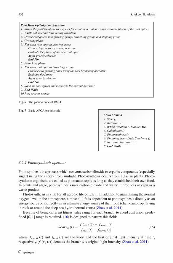
3.4.1 Root Mass Optimization (RMO) Algorithm

Root growth offers a great inspiration to propose a novel optimization algorithm. The objec-tive function is considered as growth environment of the plant roots. The apices of the initialroot forms a root mass. Each root apex can be considered as a solution of the problem. Theroots turn the direction where provides optimal soil, water, and fertilizer conditions; thus theycan reproduce. This process can be simulated as an optimizing process in the soil replacedwith an objective function. According to this view, Qi et al. (2013) proposed RMO algorithm.

Some rules make improvements in the root growth behavior of RMO:

(1) All root apices forms a root mass. Two operators, including the root regrowth and theroot branching, need to improve root growth behavior. Each root apex grows using oneof these two operators.

(2) Root mass are divided into three groups according to their fitnesses. The group withbetter fitness is called as re-growing group. The group with worse fitness, called as stopgroup, stops growing. The group, remaining from the root mass, is called as branchinggroup. The meaning of the two operators, including root growth and root branching, arelisted below (Qi et al. 2013).

123


(a) Root Growth: This operator means root apex growth in the original direction. Theroot apex can migrate to the best position where provides the optimal soil water andfertilizer conditions. This operator can be formulated using (12).

ni = xi + r + (gbest − xi ) (12)

r is a random vector whose each element is in the range of [1, 1]. ni is the newlocation of the ith root apex. xi is the original position of the ith root apex. gbest isthe root apex with the best fitness in each generation (Qi et al. 2013).

(b) Root Branching: This operator means that root apex produces a new growth pointinstead of growing along the original direction. The growth point can be producedwith a random angle β, in a random position of original root. This operator can beformulated using (13).

ni = βαxi (13)

α is a random number in the range of [0,1]. ni is the new position of ith root apex. xiis the original position of ith root apex. β can be calculated using (14).

β = λ/√

λTi λi (14)

λi is a random vector (Qi et al. 2013).

The pseudo code of RMO is listed in Fig. 6. In each generation, root apices are ranked indescending order. The selection of the root apiceswhichwill participate in the next generationuses linear descending path according to (15). This way makes a better root growth or rootbranching with better fitness performance and inhibits the growth of the bad ones. In theselection process, a percentage of root apices is selected from the front and these root apices(growing group) are allowed to grow using the root growth operator; the remaining part of theroot apices (branching group) branches using the root branching operator (Qi et al. 2013).

ratio = sRatio − (sRatio − eRation)eva

mEva(15)

eva is number of current function evaluation and mEva is maximum number of functionevaluation. sRatio is the initial percentage and eRation is the final percentage (Qi et al.2013).

3.5 Artificial Plant Optimization Algorithm (APOA)

3.5.1 Main method

An important issue for simulating phenomena of plant growth is to peer this process intothe optimization problem. Light intensity which guides to search direction in the problemspace can be seen as fitness value due to guiding growth direction of plants and supplyingsignificant energy by photosynthesis. Furthermore, a point can be seen as a branch and searchstrategy can be considered as growing curve. Because this new algorithm simulates growthmodel of plants which includes photosynthesis and phototropism mechanism, it is calledbriefly as APOA (Zhao et al. 2011).

Basic APOA pseudocode is given in Fig. 7.

123


Root Mass Optimization Algorithm1. Install the position of the root apices for creating a root mass and evaluate fitness of the root apices2. While not meet the terminating condition 3. Divide root apices into growing group, branching group, and stopping group4. Growing phase5. For each root apex in growing group

Grow using the root growing operatorEvaluate the fitness of the new root apexApply greedy selectionEnd For

6. Branching phase7. For each root apex in branching group

Produce two growing point using the root branching operatorEvaluate the fitness Apply greedy selectionEnd For

8. Rank the root apices and memorize the current best root9. End While10.Post process results

Fig. 6 The pseudo code of RMO

Fig. 7 Basic APOA pseudocode

Main Method1. Start ()2. Iteration 13. While Iteration < MaxIter Do4. Calculation()5. Photosynthesis()6. Phototropism - Light Tendency ()7. Iteration Iteration + 18. End While

3.5.2 Photosynthesis operator

Photosynthesis is a process which converts carbon dioxide to organic compounds (especiallysugar) using the energy from sunlight. Photosynthesis occurs from algae in plants. Photo-synthetic organisms are called as photoautotrophs as long as they established their own food.In plants and algae, photosynthesis uses carbon dioxide and water; it produces oxygen as awaste product.

Photosynthesis is vital for all aerobic life on Earth. In addition to maintaining the normaloxygen level in the atmosphere, almost all life is dependent to photosynthesis directly as anenergy source or indirectly as an ultimate energy source of their food (chemoautotroph livingin rock or around the deep-sea hydrothermal vents) (Zhao et al. 2011).

Because of being different fitness value range for each branch, to avoid confusion, prede-fined [0, 1] range is required. (16) is designed to narrow this field:

Scoreu (t) = f (xu (t)) − fworst (t)

fbest (t) − fworst (t)(16)

where fworst (t) and fbest (t) are the worst and the best original light intensity at time t ,respectively, f (xu (t)) denotes the branch u’s original light intensity (Zhao et al. 2011).

123


Fig. 8 Steps of photosynthesisoperator in APOA Photosynthesis ()

1. For i=1 to m Do2. Calculate the light intensity 3. Calculate the photosynthesis rate4. End Do

Photosynthesis rate plays an important role in measuring how much energy is produced.Until today,manymodels have been proposed such as rectangular hyperbolicmodel, and non-rectangular hyperbolic model. As the most important model, rectangular hyperbolic model isused successfully and extensively to simulate photosynthesis rate. For instance, rectangularhyperbolic model is used to measure the energy received for each branch.

PRu (t) = αScoreu (t) · Pmax

αScoreu (t) + Pmax− Rd (17)

where PRu (t) represents photosynthesis rate of u branch at time t , Scoreu (t) represents thelight intensity, α is the initial quantum efficiency, Pmax is the maximum net photosyntheticrate, and Rd is dark respiration rate. α, Pmax , and Rd are three parameters which control thesize of the photosynthesis rate (Zhao et al. 2011).

In each iteration, all branches grow with the energy obtained from photosynthesis accord-ing to (17). Steps of photosynthesis operator are listed as shown in Fig. 8 (Zhao et al. 2011).

3.5.3 Phototropism operator

Phototropism is usually seen in plants, but also can occur in other organisms like fungi. Thecells on the plants far from the light, have a chemical that reacts when phototropism occurs.Therefore plants have elongated cells on the farthest side from the light. Phototropism is oneof the tropismormovements that plants respond to external stimuli. Growth away from light iscalled as negative phototropism and growth towards a light source is a positive phototropism.Most plants exhibit positive phototropism, while their roots usually exhibit negative pho-totropism. Some vine shoot tips which allow growth towards to darkness, suspended solidsand climbing, exhibit negative phototropism (Zhao et al. 2011).

Each branchwill be attracted by these positions with high light intensity; therefore, branchuin iteration t will take the following action:

xu (t) = xu (t − 1) + Gp · Fu (t) · rand() (18)

where Gp is a parameter reflecting the conversion rate and used for controlling the growthrate per unit time. Fu is the growth force which is directed by photosynthesis rate, rand()

represents a random number sampled with a uniform dispersion (Zhao et al. 2011).For each branch u, Fu (t) is calculated as (19):

Fu (t) = Ftotalu (t)

‖Ftotalu (t) ‖ (19)

Ftotalu (t) is calculated as (20):

Ftotalu (t) =

∑

u �= j

Fu, j (t) (20)

and

123


Phototropism1. For i=1 to m Do2. Sort fitness values of all branches, take the better half of population as

growing-motion branches, in addition to this take the other half of population as maturing-motion branches

3. Update the positions for growing-motion branches4. Update the positions for maturing-motion branches5. End Do

Fig. 9 The steps of phototropism operator

Fu, j (t) ={0, i f ‖xu (t) − x j (t) ‖ = 0

coe · e−dimPR j (t)−e−dimPRu (t)

‖xu(t)−x j (t)‖ , otherwise(21)

where dim represents the dimensionality of the problem, coe is a parameter used to controldirection of movement.

coe ={1, i f f (xu (t)) − f

(x j (t)

)> 0,

−1, otherwise(22)

Furthermore, a small probability pm is introduced to reflect some random events

xu (t) = L + (U − L) · rand1(), i f (rand2(), pm) (23)

where L and U are the lower and upper limits in the problem space, rand1() and rand2()are two random numbers with uniform distribution, respectively. The steps of phototropismoperator are listed as shown in Fig. 9 (Zhao et al. 2011).

3.5.4 Studies with APOA

The structure prediction of Toy model of protein folding is one of the bioinformatics prob-lems. Cui et al. (2012) proposed APOA which could reach the local optimum easily andcould find the global optimum with a larger probability. Furthermore, they used splittingstrategy to improve the performance. Cui et al. (2013a) reported that in standard APOA, pho-tosynthesis operator was selected only as rectangular hyperbolic, and some light-responsivecurves could increase the photosynthesis sensitivity. They used three different curves for it.In another study, they used Gravitropism mechanism (Cui et al. 2013b). Liu and Cui (2013)proposed a new hybrid APOA based Golden Section which increased the population densityfor protein folding problem. Furthermore; a famous local search strategy, Limited MemoryBroyden–Fletcher–Shanno, was used to make an effective local search. Yu et al. 2013 pro-posed APOAwith correlation branch which was no direct communication between branchesunlike standard APOA.

Cai et al. (2012) chose seven classic models for research. These were rectangular hyper-bolic model, non-rectangular hyperbolic model, updated rectangular hyperbolic model,parabolic model, straight-line model and, two exponential curve models. Cai et al. (2013)designed binary-coded version of APOA and used this in Hydrophobic-Polar model whichwas simplest gridmodel in the protein structure prediction problem.Cui et al. (2014) designeda new dynamic local search strategy because exploitation capability is not suffice in APOA.Cai et al. (2014) indicated that in standard APOA there is no branching in each branch,

123


on the contrary, in the real tree there are many branches in each branch. They incorpo-rate two selection strategies into standard version for avoiding to this, and they tested it inDV-Hop algorithm. Zhao et al. (2011) proposed APOA to solve constrained optimizationproblems.

3.6 Sapling Growing up Algorithm (SGuA)

It is a computational method based on cultivating, growing up, and mating of saplings whichis developed for searching and optimization problems. SGuA is discovered by Karci and hiscolleagues in 2006.

As a first step for this method, in sowing sapling, there must be equal length distanceto each direction to each other. There are four operators for SGuA: Mating, Branching,Vaccinating, and Surviving (Karci 2007a, b, c; Karci and Alatas 2006).

The processes of SGuA can be explained by the following two phases:Sowing Phase—Uniformed sampling: Saplings are scattered evenly to solution space.Growing up Phase—This phase contains three operators:Mating operator aims to generate

new saplings by mating of currently available saplings. Mating operator is a global searchoperator based on data exchange between two saplings (Karci 2007a, b, c; Karci and Alatas2006).

Branching operator aims to generate new saplings from currently available saplings byusing probabilisticmethod to determine the branching position of currently available saplings.Vaccinating operator aims to generate new saplings from currently available similar saplings.Vaccinating operator is a search operator which uses similar saplings (Karci 2007a, b, c; Karciand Alatas 2006).

3.6.1 Sowing saplings

In the first place, a solution space Z is defined as Z = {z0, z1, . . . , zs−1} and it is assumedthat this solution space is in binary. In this solution space, assuming that each sapling hastwo branches, then it is in the form Z = {00, 01, 10, 11} (Karci 2007a, b, c; Karci and Alatas2006).

Firstly, two saplings S0 and S1 are arranged as S0 = {u1, u2, . . . , un} and S1 ={l1, l2, . . . , ln}. n is the length of the sapling and this case is assumed as k = 1. ui , 1 ≤ i ≤ n,is the upper bound for the corresponding variable, and li , 1 ≤ i ≤ n, is the lower bound forthe corresponding variable. Then a dividing factor, k, is determined. Firstly, k = 2 and twoextra saplings S3, S4 are derived from S0, S1. S0 is divided into two parts of equal length,by this way 4 saplings

(22 = 4

)are derived from S0. But one becomes similar to S0, and

one becomes similar to S1. Then two saplings different from S0 and S1 are derived (Karci2007a, b, c; Karci and Alatas 2006).

S3 = {l1 + (u1 − l1) ∗ r, l2 + (u2 − l2) ∗ r, . . . , ln/2

+ (un/2 − ln/2

) ∗ r, ln/2+1 + (un/2+1 − ln/2+1

) ∗ r, ln/2+2 + (un/2+2 − ln/2+2

) ∗ r}

(24)

and

S4 = {l1 + (u1 − l1) ∗ (1 − r) , l2 + (u2 − l2) ∗ (1 − r) , . . . , ln/2 + (

un/2 − ln/2)

∗ (1 − r) , ln/2+1+(un/2+1−ln/2+1

) ∗ (1 − r) , ln/2+2+(un/2+2−ln/2+2

) ∗ (1 − r)}

(25)

123


Generating Initial Garden//G, garden, I indice set and Ie enlarged indice set1. Create two saplings. Such as G[1] contains upper bounds for all variables as branches, and the other one

G[2]contains lower bounds for all variables as branches.2. Indice 33. k 24. While P is not saturated Let ie be an element of Ie and enlarged with each ie bit value and this bit value corresponds to the parti 1 While P is not saturated and all saplings are not generated for a specific value of (and 2 -2 )Do i as a bit number and ie corresponds to the enlarged value of i. Each bit of i is enlarged up to the

corresponding part of G[0] and G[1].For j1 to n DoIf, Jth bit of ie is 1 then branch of P[Index] is equal to G[1]*r.Otherwise jth branch of G[Index] is equal to G[2]*r.r is a random number in interval [0,1], and it is a real number Index Index+1i i+1

+1

Fig. 10 Generating of initial saplings in SGuA

Here, r is a random number in the range of 0 ≤ r < 1. Same method will be applied toremaining saplings in the garden by increasing the value of k. In case of k = 3, there will be6 saplings obtained from S1 (Karci 2007a, b, c; Karci and Alatas 2006).

S5 = {l1 + (u1 − l1) ∗ r, . . . , l2n/3 + (

u2n/3 − l2n/3) ∗ r, l2n/3+1

+ (u2n/3+1 − l2n/3+1

) ∗ (1 − r) , . . . , ln + (un − ln) ∗ (1 − r)}

(26)

S6 = {l1 + (u1 − l1) ∗ r, . . . , ln/3 + (

un/3 − ln/3) ∗ r, ln/3+1 + (

un/3+1 − ln/3+1)

∗ (1 − r) , . . . , l2n/3 + (u2n/3 − l2n/3

)

∗ (1 − r) , l2n/3+1 + (u2n/3+1 − l2n/3+1

) ∗ r, . . . ,}ln + (un − ln) ∗ (1 − r) (27)

S7 = {l1 + (u1 − l1) ∗ r, . . . , ln/3 + (

un/3 − ln/3) ∗ r, ln/3+1 + (

un/3+1 − ln/3+1)

∗ (1 − r) , . . . , ln + (un − ln) ∗ (1 − r)} (28)

S8 = {l1 + (u1 − l1) ∗ (1 − r) , . . . , ln/3 + (

un/3 − ln/3) ∗ (1 − r) , l2/3+1

+ (un/3+1 − ln/3+1

) ∗ r, . . . , ln + (un − ln) ∗ r}

(29)

S9 = {l1 + (u1 − l1) ∗ (1 − r) , . . . , ln/3 + (

un/3 − ln/3) ∗ (1 − r) , ln/3+1

+ (un/3+1 − ln/3+1

) ∗ r, . . . , l2n/3 + (u2n/3 − l2n/3

) ∗ r, l2n/3+1

+ (u2n/3+1 − l2n/3+1

) ∗ (1 − r) , . . . ,}ln + (un − ln) ∗ (1 − r) (30)

S10 = {l1 + (u1 − l1) ∗ (1 − r) , . . . , l2n/3 + (

u2n/3 − l2n/3) ∗ (1 − r) , l2n/3+1

+ (u2n/3+1 − l2n/3+1

) ∗ r, . . . , ln + (un − ln) ∗ r}

(31)

In binary case, current value is complemented instead of multiplying of a random value bythe current value. Sapling derivation goes on up to fulfilling the population. Pseudo code ofinitially generated saplings in SGuA is shown in the Fig. 10 (Karci 2007a, b, c; Karci andAlatas 2006).

123


Fig. 11 Mating process in SGuA

Fig. 12 Branching process in SGuA

3.6.2 Growing up saplings

Growing up phase contains three operators:Mating,Branching, andVaccinating. If the gardenG(), contains |G| number of saplings, then the current garden is replaced by the |G| numberof the best saplings of the offspring garden and the current garden. In other words, there isn’tany stochastic process in selection of the next generation garden (Karci 2007a, b, c; Karciand Alatas 2006).

(a) Mating: The purpose of the mating operator is generating a new sapling fromthe currently available saplings by replacing the currently available information with themakeshifts. S1 = {

s1,1, s1,2, . . . , s1,i , . . . , s1,n}and S2 = {

s2,1, s2,2, . . . , s2,i , . . . , s2,n}are

two saplings. The distance between S1 and S2 affects the mating process by taking place orby not taking place in the process and it depends on the distance between the current pair.Pm(S1, S2), is the mating probability of S1 and S2 saplings and it can be linear or exponen-tial. The pseudo code of mating operator is given in the Fig. 11 (Karci 2007a, b, c; Karci andAlatas 2006).

(b) Branching: S1 = {s1,1, s1,2, . . . , s1,i , . . . , s1,n

}is a sapling. If one of the branch

occurs in the point s1,i , then the probability of occurring of a branch in the point s1,i , i �= j ,can be calculated in two ways: linear and non-linear. The distance between s1,i and s1, j canbe considered as |i − j | or | j − i |. This process is shown in Fig. 12 (Karci 2007a, b, c; Karciand Alatas 2006).

(c) Vaccinating: Vaccinating process is performed between two saplings in the caseof dissimilarities of these saplings in this algorithm. Dissimilarities of saplings affects theperformance of vaccinating process and at the same time performance of vaccinating processis proportional in the case of dissimilarities of these two saplings. The pseudo code ofvaccinating operator is given in Fig. 13 (Karci 2007a, b, c; Karci and Alatas 2006).

123


Fig. 13 Vaccinating process in SGuA

Sapling Growing up Algorithm 1. t 0 2. Sowing Sapling (G(t)) 3. Computation of Objective Function (G(t)) 4. While terminating criteria are not met Do 4.1. G1(t) Mating (G(t)) 4.2. G2(t) Branching (G(t)) 4.3. G3(t) Vaccinating (G(t)) 4.4. Computation of Objective Function 4.5. G(t+1) Selection 4.6. t t+1

Fig. 14 Pseudocode of SGuA

3.6.3 SGuA

SGuA uses the similarity in the garden to generate the better saplings (Mating process). Thisis a cultural interaction process. Vaccinating process is the opposite of mating by the fact thatvaccinating operator uses the dissimilarity in the garden. That is why; it is also the oppositeof cultural interaction. Branching process is a unary operator which aims to embed the newinformation to the current solution set and to delete the information from the current solutionset. Steps of SGuA are listed in the Fig. 14.

For determining the quality of saplings, objective function is used. Objective function isdenoted as a function which considers each sapling as a solution and used as a solution for theproblem and the obtained results are the values of the objective function (Karci 2007a, b, c;Karci and Alatas 2006).

3.7 Photosynthetic Algorithm (PA)

Photosynthesis is one of the most important biochemical events. The most interesting photo-synthetic reactions are considered as “dark reactions”.Dark reactions consist of a biochemicalprocess which are combinations of Calvin–Benson cycle and photorespiration. The productof dark reaction is carbohydrates, like DHAP. PA uses the rules which regulate the conversionof carbon molecules from one substance to another in Calvin–Benson cycle, and photorespi-ration reactions. Replaced parts or shuffling are used to simulate the PA. PA is firstly proposedin 2000 byMurase. They chose analysis of the invert finite element to test the performance ofPA as a typical optimization or parameter estimation (Murase 2000). Okayama and Murase(2002) chose Vizier problem as a typical optimization problem to show the performance of

123


3 CO2

Ribulose di- phosphate (RuBP)

3-phosphoglyceric acid

1,3-diphosphoglyceric

acid

Glyceraldehyde3-phosphate




Glucose and other sugars

6 ATP

6 ADP3 ADP

3 ATP

6 NADPH

6 NADP+

6

CALVIN – BENSON CYCLE

Input

Output

Rubisco

PHASE 1: Carbon Fixation

PHASE 2: Reduction

PHASE 3: Regeneration of

Acceptor (Rubisco)

Fig. 15 Calvin–Benson cycle in PA

PA. Alatas (2011b) used PA in bioinformatics problems such as discovering association rulesin biomedical data and multiple-sequence alignment.

Fig. 15 shows the diagram of Calvin–Benson cycle. In this diagram, each row representsconversion of each molecule of each metabolite. Cycle can be separated into three phases.

(1) Fixation of CO2 by ribulose bisphosphate carboxylase (Rubisco) and formation of 3phosphoglycerate.

(2) Reduction of 3 phosphoglycerate to triose-P by the actions of glycerate-3-P kinase andNADP-dependent glyceraldehyde-P dehydrogenase.

(3) Regeneration of ribulose 1,5 bisphosphate by conversion of five C3 units into three C5units (Alatas 2011b).

Rubisco (Ribulose-1,5-bisphosphate carboxylase/oxygenize) is a bi-functional key enzy-me which fixes CO2 in chloroplasts of organisms that photosynthesize by their owncarboxylase operation. In addition to carboxylation, Rubisco can also be bind to the O2.CO2 and O2 compete with each other in the active region of Rubisco. Rubisco fixes thecarbon dioxide when carbon dioxide concentration is high. However, when oxygen concen-tration is high, Rubisco binds oxygen instead of carbon dioxide. To catalyze this oxygenactivity Rubisco’s tendency increases much with temperature than its carboxylase activity.Rubisco would prefer 100 more O2 than CO2; however, O2 concentration in the atmosphere

123


PEROXISOME

RuBP

Glycerate-3-P Glycerate

Glycolate-2-P

Glycolate

ATPADP

Pi

O2

CALVIN CYCLE

CHLOROPLAST

Fig. 16 Photorespiration in PA

is much higher than CO2’s concentration, that is why; Rubisco fixes one molecule of O2 foreach three molecule of CO2. In active parts of Rubisco, one molecule of phosphoglycerateand one molecule of phosphoglycolate form a toxic product when O2 is substituted insteadof CO2. Plants can metabolize the phosphoglycolate by photorespiration process. For thisreason, glycolate metabolism is correlated with photorespiration. Energy is required in thisprocess and also it is the reason of reduced carbon as CO2. Fig. 16 shows the part of thephotorespiratory pathway depends to Rubisco (Alatas 2011b).

In the first stage of Calvin–Benson cycle, the rules that are regulating conversion of carbonmolecules from one substance to another and the reaction located in chloroplast subcellularcompartment for photorespiration are used by PA. DHAP, the product of photosynthesis,serves to provide information strings of the algorithm. When it is not possible to improve thequality of products, then the optimum point is reached. The quality of a product is evaluatedaccording to the fitness value. Fig. 17 shows a flow diagram of the processes of the PA.

Algorithm starts with the random generation of intensity of light. Fixation rate of CO2 isevaluated according to the (32) which is based on the light intensity.

Either Calvin–Benson cycle or photorespiration cycle is selected for the next processingaccording to the fixation rate. Bits, values or parts of strings are exchanged or shuffledaccording to the recombination of carbon molecules in photosynthetic pathways in bothcycles. GAPs, the intermediate information strings, are generated after some iterations. EachGAP consists of appropriate bits, strings, or values. The fitness of these GAPs are thenevaluated. The best fitting GAP proceeds as a DHAP (Alatas 2011b).

One of the unique features of the algorithm is production of stimulation function. Ran-domly changing light intensity which alters the influence degree on renewing elements ofRuBP by photorespiration creates the stimulation. The frequency of the stimulation cycle byphotorespiration can be calculated with the CO2 fixation rate in (32).

123


• Initialize the algorithm parametersDHAPsParamaters for CO2 fixation (Affinity, Max. fixation rate)

Generate light intensity level

• Initialize the problem parameters Objective function (f(x))Decision variable (xi)Number of decision variables (N)Boundary constraints

• Calculate CO2 concentration• Determine O2 / CO2 concentration ratio• Determine CB / photorespiration

frequency ratio

Termination criteria met? END

Calvin-Benson Cycle?Photorespiration Cycle?

Photorespiration Cycle(Shuffle)

Calvin-Benson Cycle (Exchange parts)

Evalutation of DHAP

Yes

No

PhotorespirationB-C

Cycle finished? Cycle finished?

No No

Yes Yes

Fig. 17 Flow diagram of PA

C = Vmax

1 + AL

(32)

C : CO2 Fixation rateVmax : Maximum CO2 fixation rateA: Affinity of CO2

L: Light intensity

123


All parameters that are given in (32) can be determined; however, these values can beassigned within a realistic range and they don’t need to be empirical. Light intensity mightbe randomly generated by the computer when PA is executed. Time-varying actual lightintensity might be used as an alternative with on-line measuring system. For this phase,chaotic sequences may also be used. Change of light intensity as a stimuli is effective inreducing the occurring of local minimum traps in the search process. CO2 concentrationin the leaf varies according to the CO2 fixation rate. O2 and CO2 concentration ratios areevaluated to determine the ratio of calculation frequency of Calvin–Benson cycle to thephotorespiration cycle (Alatas 2011b).

3.8 Plant Growth Optimization (PGO)

PGO, which is simple but effective algorithm, is proposed to simulate plant growth with arealistic way considering the spatial occupancy, account branching, phototropism, and leafgrowth. The main purpose of the model is to select active point by comparing the morphogenconcentration for increasing the L system (Cai et al. 2008).

PGOhas somemajor differences fromnatural plant growthprocess. PGO takes the solutionspace as growth areas of artificial plant, a point of plant as a potential solution for problem.The algorithm searches optimal point in solution space according two behaviors:

1. Produce newpointswith branching to search in optimal areawhich consists of the optimalsolution;

2. The growth of leaves around the branching point to find accurate solutions in the localarea;

Considering the definitions given in the previous section, the pseudocode of PGO algo-rithm is shown in Fig. 18 (Cai et al. 2008).

Ai ={1 − f (xi )− fmin∑N

j=1[ f (x j)− fmin], f (xi ) > fmin

1, f (xi ) = fmin

i = 1, 2, . . . , N (33)

α = α/0.9 β = β/0.9 (34)

One execution of procedure from Step 2 through Step 6 is called as a generation or a cycle(Cai et al. 2008).

3.9 Root Growth Algorithm (RGA)

3.9.1 Description for growth behaviors of root system

A plant starts from a seed, and root growth is indispensable for the plant growth. All theroots of a plant can be seen as a system composed of a large number of root hairs and rootapices. In the late 1960s, Lindenmayer proposed L-systems for modeling of the plant growthprocess. L-Systems are based on simple rewrite rules and branching rules, and make a formaldefinition successfully for plant growth. In this algorithm, L-Systems are used for describinggrowth behavior of the root system (Zhang et al. 2014):

(1) A seed sprouts in the soil, and partly realizes growth as a plant stem above the soilsurface. The other part of the seed grows downward to be the plant’s root system. Thenew root hairs grow from the root apex.

(2) The newer root hairs grow from the root apices of old root hairs. Repeated behavior ofroot system is called as branching of root apices.

123


Plant Growth Optimization Algorithm 0. Start 1. Initialize:

Set NG=0 (NG is generation counter) Set NC=0 (NC is convergence counter) Set NM=0 (NM is counter of mature points) Set the upper limit of the branching points N and initialize other parameters Randomly select the branch point N0 and perform the leaf growth

2. Assign morphogen Calculate the fitness of leaf point Assign morphogen concentration of each branch using (33).

3. Branching Select randomly two critical point between 0 and 1 and dispose by (34). Produce new points with branching in four modes.

4. Selection mechanism Perform the leaf growth in all of the points Gather mature branching points the number of which is ( ) according to maturity mechanism Set Produce a new point in the center of crowded area and select the best point to substitute the crowded points. Eliminate branching points with low competition ability and select N branching point for next generation.

5. Competition Compare the current point with the mature points and get the best fitness value fmax

else Set else Set

6. Check the termination conditions: If ( ) Go to step2 else Exit

7. Stop

Fig. 18 Pseudocode of PGO Algorithm

(3) Most of the root hairs and root apices are similar. All of the plant’s root system has aself-similar structure. Root system of each plant consists of large number of root apicesand root hairs with similar structure (Zhang et al. 2014).

3.9.2 Plant morphology

The effects of the root and rhizosphere characteristics on the plant resource efficiency areimportant. Uneven concentration of nutrients in the soil makes root hair growing in differentdirections. This characteristic of root growth is associated with the model of morphologyin the biological theory. The formation of model can be considered as a complex processthat cells are differentiated and create new spatial structure. When the rhizomes of the rootsystem grows, three or four growth points with different rotation direction will be formedat each root apex. The rotation diversifies the growth direction of root apex. Root hairscontain cells whose root apices in the germinating place are undifferentiated. These cellsare regarded as fluid bags in which there are homogeneous chemical components. One ofthe chemical components is a version of growth hormone called as morphactin. Morphactin

123


concentration is a parameter of morphogenesis model. The parameter ranges between 0 and1. The morphactin concentration determines whether cells start to divide or not. When cellsstart to divide, root hairs are visible (Zhang et al. 2014).

As regards to the root growth process, in biology, there are following consequences:

(1) If the plant root system has more than one root apex which can germinate, root hairsdepends on their morphactin concentration. The probability of germination of new roothairs is higher from the root apices with larger morphactin concentration than root apiceswith less one.

(2) Morphactin concentration in the cell is not static, but it depends on its surrounding,in other words spatial distribution of nutrients in the soil. After the new root hairsgerminate and grow, morphactin concentration will be reallocated between new rootapices in parallel with new concentration of nutrients in the soil (Zhang et al. 2014).

To simulate the above process, it is assumed that the multicellular closed system is constant(considered as 1) in morphactin state space. If there are n root apices xi (i = 1, 2, . . . , n)

which are D-dimensional vectors, morphactin concentration of any cell is defined asEi (i = 1, 2, . . . , n). Morphactin concentration of each root apex can be expressed as fol-lows:

Ei = 1/ f (xi )∑ni=1 1/ f (xi )

(35)

f (xi ) is the objective function which shows the spatial distribution of nutrients in the soil. In(35), themorphactin concentration of each root apex is determined by relative position of eachpoint and environmental information in this position (objective function value). Therefore, nroot apices correspond to the n morphactin concentration values. When root hairs germinate,morphactin concentration can be changed (Zhang et al. 2014).

3.9.3 Branching of the root tips

Branching of the root apices, proposed in root growth model, is important for simulation andembodied algorithm. There are four rules for root branching as follows (Zhang et al. 2014):

(1) Plant growth begins from seed.(2) In each cycle of growth process, some excellent root apiceswhich have largermorphactin

concentration (fitness value in the embodied algorithm) are selected for branching.(3) Distance should not be close between selected root apices in order to make spatial

distribution wider and increase the diversity of fitness value.(4) If number of selected root apices is equal to predefined value, the cycle of selection

process ends (Zhang et al. 2014).

In memory, to produce a new growth point from the old root apex, the proposed modeluses following statement:

pgl j = f (x) ={xi j + (

2 × δi j − 1), j = k

xi j , j �= k(36)

k ∈ {1, 2, . . . , D} and j ∈ {1, 2, . . . , D} are randomly selected indexes. pgl (i = 1, 2, . . . ,S) are S new growth point. δi j is a random number within the range [−1, 1] (Zhang et al.2014).

123


3.9.4 Root hair growth

After new growth points are produced, root hairs begin to grow from these growth points.Root hair growth depends on its growth angle and growth length. Growth angle is a vec-tor to measure the growth direction of the root hair. Randomly generated growth angleϕi (i = 1, 2, . . . , n) can be expressed as follows:

(φ1, φ2, . . . , φD) = rand (D) (37)

ϕi = (φ1, φ2, . . . , φD)√

φ21 +φ2

2 + . . . + φ2D

(38)

The growth length of each root hair is defined as δi (i = 1, 2, . . . , n), which is an importantparameter in root growth model. Some strategies of tuning parameter can produce multipleversions of the root growth model. After growth, a new root apex can be obtained by thefollowing expression (Zhang et al. 2014):

xi = xi + δiϕi (39)

Some rules are defined as follows to simulate the trophotropism of the root system:

(1) If the morphactin concentration (fitness) of the new root apex is better than the old onein the same t cycle, the root apex will continue to grow. A new root apex in the innerloop can be expressed as:

xti = xti + δiϕi (40)

However, the number of iterations in the inner loop is a predefined value. If the numberof iterations in the inner loop is equal to a predefined value, the inner loop stops (Zhanget al. 2014).

(2) If the morphactin concentration of the new root apex is worse than the old one in thesame t cycle, the root apex will stop growing and t = t + 1. A new root apex can beexpressed as:

xt+1i = xt+1

i + δiϕi (41)

3.9.5 RGA

The proposed root growth model is embodied as RGA for simulating root growth of plantsand optimization of higher-dimensional numerical functions. The growth length of each roothair and the threshold of distance between the roots apices are important parameters for RGA.The flowchart of RGA is shown in Fig. 19. The pseudo-code for RGA is listed in Fig. 20(Zhang et al. 2014).

3.10 The Strawberry Algorithm as Plant Propagation Algorithm (PPA)

Strawberry plants belong to the rose family. Strawberry-growing industry began in Paris inthe 17th century by European diversity. Amede-Francois Freizer, who was a mathematicianand an engineer, was hired by Louis XIV in 1714 for drawing the map of South America,and he returned from Chile with Chilean strawberry plant which gives large fruits.

It is assumed that, strawberry plants, aswell as other plants, have anunderlyingpropagationstrategy. This strategy is developed over time for ensuring to survive in species. In otherwords,

123


According to RGA rules, initialize parameters and seed position

Evaluate fitness values of all root tips

Select the root tips with the larger fitness value

Branching of the selected root tips

Root hair growing and produce new root tips

The number of root tips exceeds the predefined

value

Remove the root tips with the less fitness value

Adjust root growth length

Stopping criterion is reached?

End

Yes

No

No

Yes

Fig. 19 The flowchart of the RGA

a plant makes an effort to have children in areas which provide essential nutrients and growthpotential. When a plant is in a good point, it sends lots of short runner, and when a plant isin a weak point, it sends longer runners for searching better points. Long runners are few,because they are investments. The plant may not have sufficient resource for sending manytypes of runners (Salhi and Fraga 2011).

123


Root Growth AlgorithmSet t:=0;Initialize. Randomize position of a seed and parametersWhile (the termination conditions are not met)For (each root tip x) Select S root tips pgEnd ForFor (each root tip selected pg) Produce n new growing points using (36)End For For (each root tip x) Produce new root tips using (39)End For Tune the parameter Set t:=t+1;End While

Fig. 20 Pseudocode for the RGA

It is predictable that with these observations and assumptions, strawberry plants andother plants can solve survival problem to grow in a particular environment. The mentionedapproaches here contain mapping an optimization problem onto survival optimization prob-lem of strawberry plant and adopting strategy of survival in the environment for searchingpoints in the search space which give best values and ultimately the best value.

The strawberry algorithm is an exemplar of PPA. There are two features to emit allsuccessful algorithms/heuristics for global optimization: concentration or intensification anddiversification or exploration. While diversification provides searching to prevent jammingin a review of local optimum, concentration provides local search and convergence to a localoptimum. This two features are contradictory and the success of any implementation of asearch algorithm depends on the balance between these two features (Salhi and Fraga 2011).

This strawberry approach applies concentration by sending a large number of short runnersfrom good solutions. It sends less but longer runner from the less good solutions to applydiversification. The full algorithm is presented in Fig. 21.

Asmany algorithms of this nature, PPA requires customization through the introduction ofsome auxiliary functions and assignment of values to a set of parameters. These parametersand functions for PPA are: size of population, a fitness function, the number of runners willbe created for each solution, and distance for each runners (Salhi and Fraga 2011).

PPA is based on population of shoots each of which represents a solution in the searchspace. It is assumed that each shoot is taken to be equivalent to evaluated objective function.Each shoot will subsequently be sent to explore the solution space around it. The numberof shoots is given by this parameter and it is shown as m in the algorithm. Algorithm isrepeatedly run with sending runners from shoots in each generation. This parameter providesa termination condition based on howmany times runners are transmitted, and is representedby gmax .

The solutions in the population will be sorted according to their fitness. This fitness willnaturally be a function of value of objective function. However, the real relationship betweenfitness and objective function can be tailored for discussed specific problem. Although thisis recommended for algorithm representation of fitness value supported by f (x) function,

123


Plant Propagation Algorithm Require: objective Generate a population P={ } g 1

For g 1 To Do compute { = f({ ), sort P in descending order of N create new population

For each { Do {best m only} set of runners where both the size of the set and the distance for each runner

(individually) is proportional to the fitness {append to population; death occurs by omission above}

End For P {new population}

End For Return P, the population of solutions

Fig. 21 The pseudo code of PPA

f (x) ∈ [0, 1], if not, the equations used to determine the number of runners and the distanceto be run for each runner should be modified (Salhi and Fraga 2011).

Functions are used to determine the number of runners and the distance each of whichshould be traveled by runners are described below. They require that fitness values lie strictlyin (0, 1). To ensure this, the fitness value f (x) described above is mapped:

N (x) = 1

2(tanh (4 f (x) − 2) + 1) (42)

The number of runners produced by a solution should be proportional with its fitness. Bydefault, function in (43) can be used:

nr = nmax Nir (43)

nr is the number of runners produced for generating solution i in current iteration, aftersorting; nmax is the number of runners to generate. Ni is mapped fitness of solution i ;and r ∈ [0, 1] is a randomly selected number for each individual in each generation. Thecombination of the fitness mapping function and ceiling operator provides that all solutiongenerates at least one runner, even for the fittest solutions, ones with fi (x) ≡ 0. The fittestsolutions will generate at most nmax runners (Salhi and Fraga 2011).

The distance of each runner is inversely proportional with its growth as (44):

dr, j = 2 (1 − Ni ) (r − 0.5) (44)

j = 1, . . . , n. n is the size of the search space. Each dr, j will be in the range [−1, 1]. dr, jis computed and which runner and what extend it spreads are determined. The calculateddistance will be used for updating i solution based on the limit on x j .

x∗j = x j + (

b j − a j)dr, j ) (45)

This x∗j values are set to make sure that new produced points are within the limits

[a j , b j

]

(Salhi and Fraga 2011).

123


3.10.1 Studies with PPA

Sulaiman et al. (2014) usedmodified PPA for constrained engineering optimization problems.Sulaiman et al. (2016) introduced a robust and efficient version of PPA and they providedmore effective and improved variants of it on standard continuous optimization test problemin high sizes. Birds and animals provide dispersion of the seeds into the environment, whilethey are feeding from plants. Sulaiman and Salhi presented a seed based PPA by modellingthis situation (Sulaiman and Salhi 2015).

3.11 Runner Root Algorithm (RRA)

RRA is inspired by plants such as strawberry and spider plants which are spread through theirrunners and also which develop roots and root hairs for local search for minerals and waterresources. Similar to other metaheuristics, RRA does not apply same number of functionevaluation at all iterations. More precisely, for optimal solution (exploitation procedure) inRRA, global search is performed at all iterations, while local search is performed only whenglobal search does not lead to a significant improvement in the value of cost function. Theonly similarity between this algorithm and PPA is in using the idea of runners (Merrikh-Bayat2015).

Obviously, in order to arrive at a numerical optimization algorithm inspired by plants suchas strawberry, it is needed to model the behavior of these plants by simple but effective rules.In this algorithm, it is assumed that the behaviors of such plants can be effectively modelledthrough the following three facts:

• Each strawberry mother plant spreads through their runners. These runners rise randomlyand each one leads to a new daughter plant (global search with big steps for resources).

• Each strawberry mother plant improves its roots and root hairs randomly (local searchwith relatively big steps and small steps for resources).

• Daughter strawberry plants which have access to rich resources, produce more runnersand roots, grow fast, and, therefore, cover larger areas. On the other hand, daughter plantswhich move to poor resources will probably die (Merrikh-Bayat 2015).

3.11.1 Mathematical Description of RRA

Similar to othermetaheuristic optimization algorithm, this algorithm, beginswith a uniformlydistributed random initial population, each called a mother plant in domain of the problem.The number of the mother plants is considered to be equal to Npop . Then, any mother plantat each iteration, except the fittest one, produces a daughter plant randomly in the domainof the problem (global search for better solutions). The distance of this each daughter plantfrom the mother plant is controlled by a parameter called drunner . The fittest mother plantproduces a daughter plant exactly at the same location as itself. Npop daughter plants areproduced using this procedure. It is assumed that in RRA, at each iteration each motherplant is moved to a position referred by the daughter plant. If at least one of these daughterplants provides a significant improvement in the value of cost function compared with oneof those obtained from the beginning of the algorithm, all of the mother plants required forthe next iteration are selected from these daughter plants using a combination of elite androulette wheel selection methods. More precisely, in this case, one of the necessary Npop

mother plants of the next iteration is considered to be equal to fittest daughter plant of thecurrent iteration (elite selection), and the others are obtained by applying the roulette wheel

123


method. In other words, while a significant decrease is observed in the value of cost function,the algorithm continuously examines the domain of the problem for better solutions throughrunners which improve only around the available solution. The amount of this improvementis measured by a parameter called tol.

However, if none of the resulting daughter plants leads to a pretty good value for costfunction, algorithm starts to local search procedure through roots and root hairs. In this case,the algorithm assumes that the fittest daughter plant is in the same valley as the unknownglobal best solution. Therefore, if any improvements observed by applying a random changeto each variable of this daughter plant, the algorithm accepts it. In other words, if the changewhich applies to some of the variables of the fittest daughter plant leads to a better solution,the algorithm accepts it and applies a random change to the other variable of the resulteddaughter plant. If not, the previous value of this variable is retained and a random changeis applied to the next variable of that daughter plant. This procedure is applied to all of thevariables of the fittest daughter plant. This strategy guarantees that the general movementof the fittest daughter plant, which may be the global best solution, will be towards to thenearest minimum point in the same valley. From this case, the fittest daughter plant may belocated in a valley that too flat or narrow, and both large and small random changes should beapplied to each variable of the fittest daughter plant. In conclusion, in each iteration, a globalsearch procedure is performed and a daughter plant is produced for all of the each motherplant. If none of the resulting daughter plant provides a significant improvement at the costfunction value, the variables of the fittest daughter plant are subjected to random changeswith both small and large steps (Merrikh-Bayat 2015).

The local search is not applied to all daughter plants which can significantly save thenumber of function evaluations and at all iterations. In addition to this, to increase the func-tionality, algorithm needs to be equipped with a restart strategy, because algorithm may befalling into the point trap of local optimum. For this purpose, after the global and poten-tial local search, if the relative improvement is less than tol, value of the counter calledstall_coune is incremented by 1; if not, value of the counter is equal to 0. If the value of thiscounter is equal to a predefined stall_max value, the algorithm is started with a random initialpopulation. In other words, in this case, all the solutions obtained so far are discarded, andonly the fittest solution obtained at the last iteration is memorized for comparison with thesolutions previously or subsequently obtained to determine the best solution.

For following unconstrained optimization problem min f (x)

xl ≤ x ≤ xu) (46)

f : Rm → R is m-variable cost function to be minimized, x∗ = argmin f (x) ∈ Rm is the

best global solution to be calculated, and xl , xu ∈ Rm are two vectors indicating the lower

and upper bound of variables. In case of dealing with a constrained optimization problem,standard methods can be used for converting to an unconstrained equivalent. As previouslymentioned, RRA begins with a set of Npopm-dimensional randomly generated vectors in thedomain of problem each serves as an initial mother plant. Then, in each iteration, any motherplant except the fittest one randomly generates a daughter plant and the fittest mother plantgenerates a daughter plant exactly equal to itself. Let xkmother (i) is the location of the kthmother plant k = 1, . . . , Npop at the ith iteration where x1mother (i) is the fittest daughter plantof the previous iteration and xkdaughter (i) k = 2, . . . , Npop are the mother plants selectedamong the daughter plants of the last iteration using the roulette wheel method. Thus, withusing this notation, the location of the kth daughter plant at the ith iteration, xkdaughter (i), iscalculated as:

123


xkdaughter (i) ={x1mother (i) , k = 1

xkmother (i) + drunner × rk, k = 2, . . . , Npop

(47)

where, rk ∈ Rm is a vector whose entries are random numbers with uniform in the range [-0.5,

0.5], and drunner is a scaler which represents the maximum distance of daughter plants toits mother plant. According to (47), the best daughter plant of the last iteration is consideredas a mother plant in current iteration. In addition, to calculate any daughter plant, a randomvector rk should be created (Merrikh-Bayat 2015).

The cost function is considered at the location of daughter plant as calculated in (47). Ifat least one of these daughter plant leads a significant improvement in the value of the costfunction compared with the best daughter plant of the previous iteration, for instance, if theinequality

∣∣∣∣∣∣

mink=1,...,Npop f(xkdaughter (i)

)− mink=1,...,Npop f

(xkdaughter (i − 1)

)

mink=1,...,Npop f(xkdaughter (i − 1)

)

∣∣∣∣∣∣≥ tol (48)

is satisfied, algorithm does not start to local search as long as (48) means that global searchis still effective. If the cost function is defined as if denominator of (48) has a chance to beequal to zero, the absolute difference can be used instead of the term side of it. But, if (48) isnot satisfied, local search should be performed. For this purpose, let the best daughter plantfrom those calculated is represented as xdaughter,best (i), and a vector obtained by applyinga random change to kth entry of xdaughter,best (i) is represented as xperturbed,k , for example

xperturbed,k = diag {1, 1, . . . , 1, 1 + drunner nk, 1, . . . , 1} × xdaughter,best (i) (49)

drunner is the same as before, nk (k = 1, . . . ,m) is a random number with normally dis-tributed (μ = 0 and σ = 1), and diag {1, 1, . . . , 1, 1 + drunner nk, 1, . . . , 1} is a diagonalmatrix whose all diagonal elements, except kth element, are equal to unity, and kth one isequal to 1 + drunner nk . To make local search, for k = 1, xperturbed,k is calculated from(49). If f

(xperturbed,1

)< f (xdaughter,best (i)), then xdaughter,best (i) ← xperturbed,1, else

xdaughter,best (i) is remained unchanged. Then, xperturbed,k is calculated for k = 2 from (49)using calculated xdaughter,best (i). Again if, f

(xperturbed,2

)< f (xdaughter,best (i)), then

xdaughter,best (i) ← xperturbed,2, else xdaughter,best (i) is remained unchanged. This proce-dure is repeated for all m variables of xdaughter,best (i). So far, local search with large steps(model of the root functions in nature) is completed. Now, a local search with small steps(model of root hairs function in nature) should be treated. (50) is used for this task:

xperturbed,k = diag {1, 1, . . . , 1, 1 + drootrk, 1, . . . , 1} × xdaughter,best (i) (50)

droot is a constant scalar which is considered as much smaller than drunner , xdaughter,best (i)is final result of local search with random large steps which is done before, andrk (k = 1, . . . ,m) is a random number with uniform distribution in the range [−0.5, 0.5](Merrikh-Bayat 2015).

After local search is performed (if necessary), mother plants of next iteration are selectedamong the daughter plants of current iteration using a combination of elite and roulette wheelselection. Elite selection can be as simple as the following:

x1mother (i + 1) ← xdaughter,best (i) (51)

123


Before applying roulette wheel method to select the remaining required mother plant of nextiteration, the fitness of kth daughter plant is calculated as follows:

f i t(xkdaughter (i)

)= 1

a + f(xkdaughter (i)

)− f

(xdaughter,best (i)

) (52)

a is a positive real constant controlled the selection pressure. After calculating the fitnessvalue, the selection probability of kth daughter plant as a mother plant of next iteration, pk ,is calculated as follows:

pk =f i t

(xkdaughter (i)

)

∑Npopj=1 f i t

(x jdaughter (i)

) (53)

The pseudo code of RRA is presented in Fig. 22 (Merrikh-Bayat 2015).

3.12 Path Planning Algorithm based on Plant Growth Mechanism (PGPP)

PGPP is established by extracting data processing mechanism in plant growth process. PGPPtakes the plant bud as the main computing unit to search optimal plant. The growth of buds atdifferent speeds and directions in PGPP embodies the group search capability. PGPP definesthe seed germ as starting point and the light source as destination. PGPP discretizes plantgrowth period and replaces it with iterative calculations. During each iteration, it is assumedthat plant growth behaviors remain the same. With the plant growth, the path which reachesthe light source first is the best growth path. The path is planned according to this.

PGPP extracts phototropism, negative geotropism, apical dominance, and branching inplant growth as basic rules (Zhou et al. 2016).

Phototropism is the phenomenon consisting only towards the glare of one direction lightsource, and represents the plant adaptive mechanism to poor lighting. It is induced by thechanges of the oxygen concentration in the light side and dark side. In PGPP, phototropismis summarized as follows: bud growth direction depends on the ambient light intensity in alimited reference area. Light intensity of calculation point is inversely proportional to thesquare of the distance between calculation point and destination point. Moreover, in orderto pay attention to the shadow of the barrier in the reference range, the light intensity of thepoints under it requires a correction. The calculated light intensity is used for determiningthe growth rate and the growth direction of the bud.

Negative geotropism is the characteristic that front end of plant grows away from theground and toward the sky. It is the complement of phototropism mechanism. Gravity vectorintroduces the effect of negative geotropism into PGPP. The line between the starting pointand the ending point is defined as the vertical direction. Gravity vector becomes pointed fromdestination point to starting point. Both of negative geotropism and phototropism have aneffect on the growth direction of the bud (Zhou et al. 2016).

Apical dominance is restraining effect on the growth in buds of lateral branches and issprouting caused by apical bud of main branch which includes effect on the growth angleof lateral branches. It is due to the effect of two aspects. One of these is polarity of auxintransport. The other one is different response of the bud to auxin concentration. The polaritytransport causes the buds of branches have a high oxygen concentration. Meanwhile, apicalbud of main branch has appropriate auxin concentration to promote its growth, and apicaldominance occurs. The transport amount of auxin polarity is determined by the differencesbetween ages of branches.

123


Fig. 22 The pseudo code of RRA

Branchmeans sprouting newbranches frommain branch to absorb the sunlight. Branchingis used to perform the search path diversity. It provides to PGPP for finding optimal pathrather than a suboptimal path. When branches grow to branching age, PGPP judges whetherto branch in a random way. The growth direction of the bud in the new branch depends onlight intensity distribution of bud in original branch. The light intensity of new bud in newbranch is randomly selected from the top five large light intensity values of original bud(Zhou et al. 2016).

123


Fig. 23 The flowchart of PGPP

Start

Initialize

Light Intensity Calculation

Random Branch

Growth Vector Calculation

Plant Growth

Reach Target?

End

Yes

No

Output Path

3.12.1 Basic processes

PGPP includes six basic steps. The flowchart of PGPP is shown in Fig. 23.

Step 1: Initialization. Initialize variables such as plant and light intensity. Indicate themap data. Set the starting point as the growth point of the first bud.Step 2: Calculation of light intensity. Calculate the light intensity in the reference range.Step 3: Random branching. If themain branch reaches the branching condition, randomlycreate new branches.Step 4: Calculation of growth vector. Calculate growth vector of light intensity and auxinconcentration of the all buds. Then, to obtain the new growth vector, calculate weightedsum of the last period growth vector, gravitational growth vector, and light intensitygrowth vector.

123


Step 5: Plant growth. Each bud performs cell division until a new cell reaches the destina-tion according to its growth vector. If any cell reaches the destination, route search endsand then proceeds to the next step. Otherwise, all the buds no sooner finish the growthof this period than go back to the second step.Step 6: Way output. Way planning ends. The optimal way can be established from thestart point to the destination point through being searched the parent cell by cell (Zhouet al. 2016).

3.13 Rooted Tree Optimization (RTO)

3.13.1 Roots look for water

A root has a limited capacity, but a group of roots can find together the best location to getwater and their density positions around this location or around the way which connectsthe water resource with the plant. To create the algorithm, a presumptive behavior whichis a way how the roots decide together, is added for selecting their orientation according tothe wetness degree where the root head is in. These roots move randomly, but when one ormore of them finds the wetness, to get the original location of the water and to strengthentheir presence around this location, they call other roots. According to RTO algorithm, thesolutions remote from water resources are omitted or replaced with the new roots orientedrandomly. Moreover, the solutions remote from water resources can be changed by the rootswhich are next to the best root of the previous generation. The roots with significant wetnessdegree retain their orientation (Labbi et al. 2016).

3.13.2 RTO

Similar to other methods, the proposed algorithm starts by randomly creating an initialpopulation. Some terms used for determining how initial population of RTO algorithmmovesto a new one, are:

• Root: a candidate or proposed solution• Degree of wetness (Dw): a term that evaluates a candidate and gives fitness degree

between population segments (Labbi et al. 2016).

3.13.2.1 The rate of the nearest root to water (Rn)It is the rate which represents number of candidates according to the total population that

need rally around the wetter locations. The new population of root, which is the closest tothe water is calculated as follows:

xnew (i, I t + 1) = xbest (I t) + c1 × Dw (i) × randn × l/ (N × I t) (54)

I t is a step in the iteration. xnew (I t + 1) is the new candidate for the iteration (I t + 1);xbest (I t) is the best solution from the previous generation. i is the number of candidate, Nis the population scale.l is the upper bound of parameter, and randn is a random number inthe range of [−1, 1]. Then a new point xnew is lower and upper bounded (Labbi et al. 2016).

3.13.2.2 The rate of the continuous root in its orientation (Rc)It is the rate of members which are directed from the previous way because of closing to

the water. The new population of the random root is calculated as:

123


xnew (i, I t + 1) = x (i, I t) + c2 × Dw (i) × rand ×(xbest (I t) − x (i, I t)

)(55)

x (I t) is the previous candidate for the iteration I t , and rand is a random number in therange of [0, 1] (Labbi et al. 2016).

3.13.2.3 The rate of the random root (Rr )It is the rate which represents the number of candidates according to the total population

that is randomly distributed at search area, in order to increase the uptake rate of the generalsolution. In addition, it changes roots with a weak wetness degree from the last generation.The new population of random root is calculated as:

xnew (i, I t + 1) = xr (I t) + c3 × Dw (i) × randn × l/I t (56)

xr is randomly selected individual from theprevious generation; c1, c2, and c3 are configurableparameters.

Rn, Rr , and Rc ratios are experimentally determined according to the investigated prob-lem. These ratios are considered as variables affecting the convergence. Rr value is alwayssmall compared with others, because it aims to reserve the randomness to be far from localsolutions. Dw value is added from the search function of roots for determining a search areaaccording to candidate force (Labbi et al. 2016).

3.13.3 RTO algorithm

The steps of RTO algorithm can be summarized as follows:

Step 1: Randomly create the first generation which consists of N candidates withinvariable limits in the search area, and set the numerical values of Rn , Rr , and Rc ratios.Step 2: Evaluate the whole population members for measuring Dw as following:

Dw (i) =⎧⎨

⎩

fimax(fi)

for the maximum objective

1 − fimax(fi)

for the minimum objective, i = 1, 2, . . . , N (57)

or directly use the fitness regardless of the suitable formula.Step 3: Reproduce and replace with the new population. According to Rn , Rr , and Rc

reorder the population using the (54)-(56), according to wetness degree to replace withthe new population.Step 4: If the termination conditions are not reached, go back to step 2 (Labbi et al. 2016).

Fig. 24 shows the pseudocode of RTO algorithm. It includes two basic procedures: (a)start (b) repeated body until termination conditions cannot be reached.

4 Discussions

Depending on the source of inspiration, all of the plant based metaheuristic algorithms in theliterature have been searched and collected for the first time to present a relatively compre-hensive list and to inspire further research. One of the research works in the related literatureconsist of comparing one of these plant based algorithms to the other nature inspired algo-rithms. Theseworks have experimentally shown that someplant intelligence based algorithmsare better than other nature inspired methods although it is still not quite understood why.Especially, the older plant intelligence based algorithms have been compared with GA andPSO.Algorithmswhich lack certain basic capabilities such as themixing and diversity among

123


RTO AlgorithmBegin//InitializationSet the rates Rn, Rr, and Rc parametersGive the maximum number of iterations: MaxIte, and the population scale: the RTOsizeSet iteration counter it=1Generate the initial population X(1) randomly within the search range of (Xmin, Xmax) //Loop Repeat

Evaluate the Dwi for each root //DW: Fitness, root: IndividualReorder the population according to the witness degreeIdentify the candidate according to the wetness place Xbest //the global best in whole populationFor i=1 : Rr×theRTOsize Do

Selected individual Xr(it) randomly from the current population

Xi(it+1)=Xr

(it)+c1×DWi×randn×|Xmin +Xmax|/itEnd ForFor i=Rr×theRTOsize+1 To (Rr+Rn)×theRTOsize Do

Xi(it+1)=Xbest+c3×DWi×randn×|Xmin +Xmax|/(it×theRTOsize)

End ForFor i=(1-Rc)×theRTOsize+1 To theRTOsize Do

Xi(it+1)=Xi

(it)+c1×DWi×rand×(Xbest-Xi(it))

End ForUpdate Xbest

it=it+1Until For a stop ciriterion is not satisfied //&it<MaxIteEnd

Fig. 24 The pseudocode of RTO algorithm

the solutions can be thought as badly designed. Most of the plant based metaheuristic searchand optimization algorithms which have been searched and collected for the first time in thispaper have been developed relatively more recently and there is not any work about compar-ing all of their performances in the selected complex benchmark or engineering problemssatisfying the equal conditions. Equal conditions mean using the same starting and termi-nation criterion, equal number of starting search points, the same benchmark function withequal dimensions and intervals for these dimensions, same hardware running the algorithms,same programming languages, and maybe the same programmer. Thus, it can be concludedthat there is not a single software available for evaluating all these new plant based algorithmsover different types of benchmark functions; this provides an opportunity for the researchcommunity to develop the unified software that could be used to simulate the performanceof these algorithms over benchmark problems used for search and optimization.

Software which can be developed in near future can also be extended for solving variousother types of discrete, combinatorial, NP hard, multi-objective, complex optimization prob-lems etc. It can be concluded that metaheuristic algorithms inspired from plant behaviorshave much room to grow since this research community is quite young. Thus, this paperwould act as a boon to the research community in identifying the research prospects in thefield of metaheuristic optimization.

If more works are performed in relatively more recent plant based algorithms, they canhave bothmixing and diversity control so that the algorithms can explore the vast search spaceefficiently, while converge relatively more quickly. Some good and relatively old algorithmssuch as FPA and SGuA have both global search and intensive local search capabilities, which

123


balance the exploration and exploitation, and they seem partly more efficient in unimodaland multimodal functions or problems. Their solution quality in terms of mean objectivevalue is much better and the value of the standard deviation indicates that the results obtainedfrom them are more consistent due to the huge number of works on their performances.More works should be performed for more recent algorithms such as RTO and PGPP whichhave been proposed in 2016, RRA and PPA which have been proposed in 2015 in orderto increase the performance in terms of convergence, precision, robustness, and generalperformance.

In future, more comprehensive evaluation of all plant inspired metaheuristic algorithmswith graphical and tabular analysis may be focused on. Their variants containing multi objec-tivity, dynamic parameter selection, different initial populationmethods, different terminationcriterion, discrete versions, and their hybrids with other metaheuristic or heuristic meth-ods may be proposed for efficient solutions as these plant based metaheuristic algorithmshave high potential to solve various search and optimization problems in different areas.Researchers should be encouraged to implement a detailed performance analysis of thesealgorithms truly to pick up the best methods for different types of hard problems. Therefore,searching and collecting all of the plant based metaheuristic algorithms in the literature forthe first time and inspiring more research to gain better insight into efficient algorithms andsolve large-scale real-world problems has been aimed with this paper.

5 Conclusions

Although there are many successful search and optimization algorithms and techniques inthe literature; design, development, and implementation of new techniques is an importanttask under the philosophy of improvement in the scientific field and always searching todesign better. Best algorithm that gives the best results for all of the problems have not yetbeen designed, that is why constantly new artificial intelligence optimization algorithms areproposed or some efficient additions or modifications have been performed to the existingalgorithms.

In recent years, researchers have shown that plants exhibit intelligent behaviors. Althoughthere are thirteen different plant intelligence based metaheuristic search and optimizationalgorithms, they are not known by the researchers of the related area. However, they seemto be very popular in solving of high-dimensional and hard problems due to their efficiencyand robustness.

In this paper, all of the metaheuristic algorithms inspired from plant intelligence havebeen firstly searched, collected, and their properties are introduced in a smooth way. In thisway, the main algorithm and source of inspiration are introduced. Besides, the basic steps ofthe plant intelligence based optimization algorithms are demonstrated. Consequently, studiesabout related algorithms are shown to reveal how those algorithms helped solving of complexproblems.

This paper will help the related researchers to rapidly gain information about novel tech-niques, the differences between these techniques, and adopting them for different types ofcomplex search and optimization problems.

123


References

Abdel-Raouf O, Abdel-Baset M, El-henawy I (2014a) An improved flower pollination algorithm with chaos.Int J Edu Manage Eng 4:1

Abdel-Raouf O, Abdel-Baset M, El-henawy I (2014b) A new hybrid flower pollination algorithm for solvingconstrained global optimization problems. Int J Appl Op Res 4:1–13

Abdel-RaoufO, El-Henawy I,Abdel-BasetM (2014c)Anovel hybrid flower pollination algorithmwith chaoticharmony search for solving sudoku puzzles. Int J Mod Edu Comput Sci 6:38

Ahmadi M, Mojallali H (2012) Chaotic invasive weed optimization algorithm with application to parameterestimation of chaotic systems. Chaos Solitons fractals 45:1108–1120

Alatas B (2011a) ACROA: artificial chemical reaction optimization algorithm for global optimization. ExpertSyst Appl 38:13170–13180

Alatas B (2011b) Photosynthetic algorithm approaches for bioinformatics. Expert Syst Appl 38:10541–10546Atashpaz-Gargari E, LucasC (2007a) Imperialist competitive algorithm: an algorithm for optimization inspired

by imperialistic competition. In: 2007 IEEE congress on evolutionary computation. 25–28 Sept. pp 4661–4667. doi:10.1109/CEC.2007.4425083

Atashpaz-Gargari E, LucasC (2007b) Imperialist competitive algorithm: an algorithm for optimization inspiredby imperialistic competition. In: IEEE congress on evolutionary computation. CEC 2007, pp 4661–4667.doi:10.1109/CEC.2007.4425083

Basak A, Pal S, Das S, Abraham A, Snasel V (2010) A modified invasive weed optimization algorithm fortime-modulated linear antenna array synthesis. In: IEEE congress on evolutionary computation (CEC).18–23 July. pp 1–8. doi:10.1109/CEC.2010.5586276

Borji A (2007) A new global optimization algorithm inspired by parliamentary political competitions.In: MICAI 2007: advances in artificial intelligence. Springer, pp 61–71. doi:10.1007/978-3-540-76631-5_7

Cai W, Yang W, Chen X (2008) A global optimization algorithm based on plant growth theory: plant growthoptimization. In: 2008 International conference on intelligent computation technology and automation(ICICTA). 20–22 Oct. pp 1194–1199. doi:10.1109/ICICTA.2008.416

Cai X, Fan S, Tan Y (2012) Light responsive curve selection for photosynthesis operator of APOA. Int JBio-Inspired Comput 4:373–379. doi:10.1504/IJBIC.2012.051411

Cai X, Li P, Wu X (2014) Artificial plant optimization algorithm with double selection strategies for DV-Hop.Sensor Lett 12:1383–1387. doi:10.1166/sl.2014.3356

Cai X,WuX,Wang L, KangQ,WuQ (2013) Hydrophobic-polar model structure prediction with binary-codedartificial plant optimization algorithm. J Comput Theor Nanosci 10:1550–1554. doi:10.1166/jctn.2013.3439

Cheng M, Dawei D, Pandeng Z, Jia L, Fei L (2011) A novel method using PFA in parameters turning of PIDcontroller of high-order system. In: 2011 IEEE international conference on information and automation(ICIA). 6–8 June, pp 662–665. doi:10.1109/ICINFA.2011.5949076

Chu S-C, Tsai P-W, Pan J-S (2006) Cat swarm optimization. In: PRICAI 2006: trends in artificial intelligence.Springer. pp 854–858. doi:10.1007/978-3-540-36668-3_94

Cui Z, Fan S, Zeng J, Shi Z (2013) Artificial plant optimisation algorithm with three-period photosynthesis.Int J Bio-Inspired Comput 5:133–139. doi:10.1504/IJBIC.2013.053507

Cui Z, Liu D, Zeng J, Shi Z (2012) Using splitting artificial plant optimization algorithm to solve toy modelof protein folding. J Comput Theor Nanosci 9:2255–2259. doi:10.1166/jctn.2012.2647

Cui Z, Liu W, Dai C, Chen W (2014) Artificial plant optimization algorithm with dynamic local search foroptimal coverage configuration. Sensor Lett 12:118–122. doi:10.1166/sl.2014.3238

Cui Z, Liu X, Liu D, Zeng J, Shi Z (2013) Using gravitropism artificial plant optimization algorithm to solvetoy model of protein folding. J Comput Theor Nanosci 10:1540–1544. doi:10.1166/jctn.2013.3437

Cura T (2008) Modern sezgisel teknikler ve uygulamaları. Papatya Yayıncılık,Dorigo M, Maniezzo V, Colorni A (1991) The ant system: an autocatalytic optimizing process. Technical

ReportGeemZW,Kim JH, LoganathanG (2001)A newheuristic optimization algorithm: harmony search. Simulation

76:60–68Ghasemi M, Ghavidel S, Akbari E, Vahed AA (2014) Solving non-linear, non-smooth and non-convex opti-

mal power flow problems using chaotic invasive weed optimization algorithms based on chaos. Energy73:340–353. doi:10.1016/j.energy.2014.06.026

Ghasemi M, Ghavidel S, Rahmani S, Roosta A, Falah H (2014b) Novel hybrid algorithm of imperialistcompetitive algorithm and teaching learning algorithm for optimal power flow problemwith non-smoothcost functions. Eng Appl Artif Intell 29:54–69. doi:10.1016/j.engappai.2013.11.003

123

http://dx.doi.org/10.1109/CEC.2007.4425083



http://dx.doi.org/10.1007/978-3-540-76631-5_7

http://dx.doi.org/10.1007/978-3-540-76631-5_7

http://dx.doi.org/10.1109/ICICTA.2008.416

http://dx.doi.org/10.1504/IJBIC.2012.051411

http://dx.doi.org/10.1166/sl.2014.3356

http://dx.doi.org/10.1166/jctn.2013.3439


http://dx.doi.org/10.1109/ICINFA.2011.5949076

http://dx.doi.org/10.1007/978-3-540-36668-3_94



http://dx.doi.org/10.1166/sl.2014.3238


http://dx.doi.org/10.1016/j.energy.2014.06.026

http://dx.doi.org/10.1016/j.engappai.2013.11.003


Ghasemi M, Taghizadeh M, Ghavidel S, Abbasian A (2016) Colonial competitive differential evolution: anexperimental study for optimal economic load dispatch. Appl Soft Comput 40:342–363. doi:10.1016/j.asoc.2015.11.033

GhasemiM, TaghizadehM, Ghavidel S, Aghaei J, Abbasian A (2015) Solving optimal reactive power dispatchproblem using a novel teaching-learning-based optimization algorithm. EngAppl Artif Intel 39:100–108.doi:10.1016/j.engappai.2014.12.001

He S,WuQH, Saunders JR (2006) A novel group search optimizer inspired by animal behavioural ecology. In:2006 IEEE international conference on evolutionary computation. 1272–1278. doi:10.1109/CEC.2006.1688455

He S, Wu QH, Saunders JR (2009) Group search optimizer: an optimization algorithm inspired by animalsearching behavior. IEEE Trans Evolut Comput 13:973–990. doi:10.1109/TEVC.2009.2011992

Holland J (1975) Adaption in natural and artificial systems. The University of Michigan Press, Ann ArborJin X, Reynolds RG (1999) Using knowledge-based evolutionary computation to solve nonlinear constraint

optimization problems: a cultural algorithm approach. In: 1999 IEEE congress on evolutionary compu-tation, CEC 99. vol. 3. pp. 1678. doi:10.1109/CEC.1999.785475

Kanagasabai L, RavindhranathReddy B (2014) Reduction of real power loss by using fusion of flower polli-nation algorithm with particle swarm optimization. J Inst Ind Appl Eng 2:97–103

Karaboga D (2011) Yapay Zeka Optimizasyon Algoritmaları. Nobel Yayın DagıtımKarci A (2007a) Human being properties of saplings growing up algorithm. In: IEEE international conference

on computational cybernetics. ICCC2007. 19–21Oct. pp 227–232. doi:10.1109/ICCCYB.2007.4402039Karci A (2007b) Natural inspired computational intelligence method: saplings growing up algorithm. In: IEEE

international conference on computational cybernetics. ICCC2007. 19–21Oct. pp 221–226. doi:10.1109/ICCCYB.2007.4402038

Karci A (2007c) Theory of saplings growing up algorithm. In: adaptive and natural computing algorithms.lecture notes in computer science. Berlin: Springer. Heidelberg. pp 450–460. doi:10.1007/978-3-540-71618-1_50

KarciA,AlatasB (2006) ThinkingCapability of saplings growing up algorithm. In: Intelligent data engineeringand automated learning—IDEAL 2006. vol 4224. Lecture notes in computer Science. Springer, Berlin,pp 386–393. doi:10.1007/11875581_47

Karimkashi S, Kishk AA (2010) Invasive weed optimization and its features in electromagnetics. IEEE TransAntennas Propag 58:1269–1278. doi:10.1109/TAP.2010.2041163

Kashan AH (2009) League championship algorithm: a new algorithm for numerical function optimization.In: IEEE international conference of soft computing and pattern recognition. SOCPAR’09. pp 43–48.doi:10.1109/SoCPaR.2009.21

Kaveh A, Talatahari S (2010) A novel heuristic optimization method: charged system search. Acta Mechanica213:267–289. doi:10.1007/s00707-009-0270-4

Kennedy J, Eberhart R (1995) Particle swarm optimization. In: IEEE international conference on neuralnetworks. Piscataway, NJ. pp 1942–1948

Kong X, Chen YL, Xie W, Wu X (2012) A novel paddy field algorithm based on pattern search method. In:2012 International conference on information and automation (ICIA). 6–8 June. pp 686–690. doi:10.1109/ICInfA.2012.6246764

Kostrzewa D, Josinski H (2009) The comparison of an adapted evolutionary algorithm with the invasive weedoptimization algorithm based on the problem of predetermining the progress of distributed data mergingprocess. In: Man-Machine Interactions. vol 59. Adv Intel Soft Comput. Berlin: Springer Heidelberg. pp505–514. doi:10.1007/978-3-642-00563-3_53

Labbi Y, Attous DB, Gabbar HA, Mahdad B, Zidan A (2016) A new rooted tree optimization algorithm foreconomic dispatch with valve-point effect. Int J Electr Power Energy Syst 79:298–311. doi:10.1016/j.ijepes.2016.01.028

Lam AYS, Li VOK (2010) Chemical-reaction-inspired metaheuristic for optimization. IEEE Trans EvolutComput 14:381–399. doi:10.1109/TEVC.2009.2033580

Lenin K (2014) Shrinkage of active power loss by hybridization of flower pollination algorithm with chaoticharmony search algorithm. Control Theory Inform 4:31–38

Li Y, Yang F, OuYang J, Zhou H (2011) Yagi-Uda antenna optimization based on invasive weed optimizationmethod. Electromagnetics 31:571–577. doi:10.1080/02726343.2011.621108

Liu D, Cui Z (2013) Protein folding structure prediction with artificial plant optimization algorithm basedgolden section and limited memory Broyden–Fletcher–Goldfarb–Shanno. J Bionanosci 7:114–120.doi:10.1166/jbns.2013.1103

Łukasik S, Kowalski P (2015) Study of flower pollination algorithm for continuous optimization. In: Intelligentsystems’2014. vol 322.Advances in intelligent systems and computing. Springer International Publishing.pp 451–459. doi:10.1007/978-3-319-11313-5_40

123

http://dx.doi.org/10.1016/j.asoc.2015.11.033


http://dx.doi.org/10.1016/j.engappai.2014.12.001



http://dx.doi.org/10.1109/TEVC.2009.2011992


http://dx.doi.org/10.1109/ICCCYB.2007.4402039



http://dx.doi.org/10.1007/978-3-540-71618-1_50

http://dx.doi.org/10.1007/978-3-540-71618-1_50

http://dx.doi.org/10.1007/11875581_47

http://dx.doi.org/10.1109/TAP.2010.2041163

http://dx.doi.org/10.1109/SoCPaR.2009.21

http://dx.doi.org/10.1007/s00707-009-0270-4

http://dx.doi.org/10.1109/ICInfA.2012.6246764

http://dx.doi.org/10.1109/ICInfA.2012.6246764

http://dx.doi.org/10.1007/978-3-642-00563-3_53

http://dx.doi.org/10.1016/j.ijepes.2016.01.028

http://dx.doi.org/10.1016/j.ijepes.2016.01.028


http://dx.doi.org/10.1080/02726343.2011.621108

http://dx.doi.org/10.1166/jbns.2013.1103

http://dx.doi.org/10.1007/978-3-319-11313-5_40


Mallahzadeh ARR, Oraizi H, Davoodi-Rad Z (2008) Application of the invasive weed optimization techniquefor antenna configurations. Prog Electromag Res 79:137–150. doi:10.2528/PIER07092503

Maniezzo V, Stützle T, Voss S (2009) Matheuristics: hybridizing metaheuristics and mathematical program-ming, vol 10. Springer, New York

Mehrabian AR, Lucas C (2006) A novel numerical optimization algorithm inspired from weed colonization.Ecol Inform 1:355–366. doi:10.1016/j.ecoinf.2006.07.003

Mehrabian AR, Yousefi-Koma A (2007) Optimal positioning of piezoelectric actuators on a smart fin usingbio-inspired algorithms. Aerosp Sci Technol 11:174–182. doi:10.1016/j.ast.2007.01.001

Merrikh-Bayat F (2015) The runner-root algorithm: a metaheuristic for solving unimodal and multimodaloptimization problems inspired by runners and roots of plants in nature. Appl Soft Comput 33:292–303.doi:10.1016/j.asoc.2015.04.048

Monavar FM, Komjani N (2011) Bandwidth enhancement of microstrip patch antenna using jerusalem cross-shaped frequency selective surfaces by invasive weed optimization approach. Prog Electromagn Res121:103–120. doi:10.2528/PIER11051305

MuraseH (2000) Finite element inverse analysis using a photosynthetic algorithm. Comput Electr Agr 29:115–123. doi:10.1016/S0168-1699(00)00139-3

NikoofardAH,Hajimirsadeghi H, Rahimi-KianA, Lucas C (2012)Multiobjective invasiveweed optimization:application to analysis of pareto improvement models in electricity markets. Appl Soft Comput 12:100–112. doi:10.1016/j.asoc.2011.09.005

Okayama T, Murase H (2002) Solution for N-Queens problem using a photosynthetic algorithm. In: 15thTriennial World Congress IFAC

Platt GM (2014) Computational experiments with flower pollination algorithm in the calculation of doubleretrograde dew points. Int Rev Chem Eng 6(2):95–99

Pourjafari E, Mojallali H (2012) Solving nonlinear equations systems with a new approach based on invasiveweed optimization algorithm and clustering. Swarm Evolut Comput 4:33–43. doi:10.1016/j.swevo.2011.12.001

Prathiba R, Moses MB, Sakthivel S (2014) Flower pollination algorithm applied for different economic loaddispatch problems. Int J Eng Technol 6:1009–1016

Premaratne U, Samarabandu J, Sidhu T (2009) A new biologically inspired optimization algorithm. in: 2009international conference on industrial and information systems (ICIIS). 28–31 Dec. pp 279–284. doi:10.1109/ICIINFS.2009.5429852

Qi X, Zhu Y, Chen H, Zhang D, Niu B (2013) An idea based on plant root growth for numerical optimization.In: Intelligent computing theories and technology. vol 7996. Lecture notes in computer science. Springer,pp 571–578. doi:10.1007/978-3-642-39482-9_66

Rad HS, Lucas C (2007) A recommender system based on invasive weed optimization algorithm. In: IEEEcongress on evolutionary computation, CEC 2007. 25–28 Sept. pp 4297–4304. doi:10.1109/CEC.2007.4425032

Rao RV, Savsani VJ, Vakharia DP (2011) Teaching-learning-based Optimization: a novel method for con-strained mechanical design optimization problems. Computer-Aided Des 43:303–315. doi:10.1016/j.cad.2010.12.015

Rashedi E, Nezamabadi-Pour H, Saryazdi S (2009) GSA: a gravitational search algorithm. Inf Sci 179:2232–2248. doi:10.1016/j.ins.2009.03.004

Roy GG, Das S, Chakraborty P, Suganthan PN (2011) Design of non-uniform circular antenna arrays using amodified invasive weed optimization algorithm. IEEE Trans Antennas Propag 59:110–118. doi:10.1109/TAP.2010.2090477

Sakib N, Kabir M, Subbir M, Alam S (2014) A comparative study of flower pollination algorithm and batalgorithm on continuous optimization problems. Int J Appl Inf Syst 7:19–20

SalemSA (2012)BOA: a novel optimization algorithm. In: IEEE2012 InternationalConference on engineeringand technology (ICET). pp 1–5. doi: 10.1109/ICEngTechnol.2012.6396156

Salhi A, Fraga ES (2011) Nature-inspired optimisation approaches and the new plant propagation algorithm.In: The international conference on numerical analysis and optimization (ICeMATH ’11). Yogyakarta,Indonesia

Shah-Hosseini H (2009) The intelligent water drops algorithm: a nature-inspired swarm-based optimizationalgorithm. Int J Bio-Inspired Comput 1:71–79. doi:10.1504/IJBIC.2009.022775

Simon D (2008) Biogeogr Based Optim. IEEE Trans Evolut Comput 12:702–713. doi:10.1109/TEVC.2008.919004

Storn R, Price K (1995) Differential evolution: a simple and efficient adaptive scheme for global optimizationovercontinuous spaces. Technical Report TR-95-012. vol 3. ICSI Berkeley

Sulaiman M, Salhi A (2015) A seed-based plant propagation algorithm: the feeding station model. Sci WorldJ 2015:16. doi:10.1155/2015/904364

123

http://dx.doi.org/10.2528/PIER07092503

http://dx.doi.org/10.1016/j.ecoinf.2006.07.003

http://dx.doi.org/10.1016/j.ast.2007.01.001



http://dx.doi.org/10.1016/S0168-1699(00)00139-3


http://dx.doi.org/10.1016/j.swevo.2011.12.001

http://dx.doi.org/10.1016/j.swevo.2011.12.001

http://dx.doi.org/10.1109/ICIINFS.2009.5429852

http://dx.doi.org/10.1109/ICIINFS.2009.5429852

http://dx.doi.org/10.1007/978-3-642-39482-9_66



http://dx.doi.org/10.1016/j.cad.2010.12.015

http://dx.doi.org/10.1016/j.cad.2010.12.015

http://dx.doi.org/10.1016/j.ins.2009.03.004



http://dx.doi.org/10.1109/ICEngTechnol.2012.6396156




http://dx.doi.org/10.1155/2015/904364


Sulaiman M, Salhi A, Fraga ES, Mashwani WK, Rashidi MM (2016) The plant propagation algorithm:modifications and implementation. Sci Int 28

Sulaiman M, Salhi A, Selamoglu BI, Kirikchi OB (2014) A plant propagation algorithm for constrainedengineering optimisation problems. Math Probl Eng 2014:10. doi:10.1155/2014/627416

Sundareswaran K, Nayak PS, Sankar P, Kumar VV (2014) Inverter harmonic elimination through flowerpollination enhanced genetic algorithm. Int J Adv Trends Comput Sci Eng 3:342–348

Wang G-G, Deb S, Cui Z (2015) Monarch butterfly optimization. Neural Comput Appl. doi:10.1007/s00521-015-1923-y

Wang R, Zhou Y (2014) Flower pollination algorithmwith dimension by dimension improvement. Math ProblEng. doi:10.1155/2014/481791

Wang S, Dai D, Hu H, Chen YL, Wu X (2011) RBF neural network parameters optimization based on paddyfield algorithm. In: 2011 IEEE international conference on information and automation (ICIA). 6–8 June.pp 349–353. doi:10.1109/ICINFA.2011.5949015

Yang X-S (2012) Flower Pollination Algorithm for global optimization. In: Unconventional computation andnatural computation. Springer. pp 240–249. doi:10.1007/978-3-642-32894-7_27

Yang X-S, KaramanogluM, He X (2013)Multi-objective flower algorithm for optimization. Procedia ComputSci 18:861–868. doi:10.1016/j.procs.2013.05.251

Yang X-S, Karamanoglu M, He X (2014) Flower pollination algorithm: a novel approach for multiobjectiveoptimization. Eng Optim 46:1222–1237. doi:10.1080/0305215X.2013.832237

YangXS, Suash D (2009) Cuckoo search via levy flights. In:World Congress on nature & biologically inspiredcomputing. NaBIC 2009. 9–11 Dec. pp 210–214. doi:10.1109/NABIC.2009.5393690

Yu B, Cui Z, Zhang G (2013) Artificial plant optimization algorithm with correlation branches. J BioinformIntel Control 2:146–155. doi:10.1166/jbic.2013.1039

Zaharis ZD, Skeberis C, Xenos TD (2012) Improved antenna array adaptive beamforming with low side lobelevel using a novel adaptive invasive weed optimization method. Prog Electromag Res 124:137–150.doi:10.2528/PIER11120202

Zhang H, Zhu Y, Chen H (2014) Root growth model: a novel approach to numerical function optimizationand simulation of plant root system. Soft Comput 18:521–537. doi:10.1007/s00500-013-1073-z

Zhao Z, Cui Z, Zeng J, Yue X (2011) Artificial plant optimization algorithm for constrained optimizationproblems. In: 2011 Second international conference on innovations in bio-inspired computing and appli-cations (IBICA). 16–18 Dec.. pp 120–123. doi:10.1109/IBICA.2011.34

Zhou Y, Wang Y, Chen X, Zhang L, Wu K (2016) A Novel path planning algorithm based on plant growthmechanism. Soft Comput 1–11: doi:10.1007/s00500-016-2045-x

123

http://dx.doi.org/10.1155/2014/627416

http://dx.doi.org/10.1007/s00521-015-1923-y

http://dx.doi.org/10.1007/s00521-015-1923-y

http://dx.doi.org/10.1155/2014/481791

http://dx.doi.org/10.1109/ICINFA.2011.5949015

http://dx.doi.org/10.1007/978-3-642-32894-7_27

http://dx.doi.org/10.1016/j.procs.2013.05.251

http://dx.doi.org/10.1080/0305215X.2013.832237

http://dx.doi.org/10.1109/NABIC.2009.5393690

http://dx.doi.org/10.1166/jbic.2013.1039


http://dx.doi.org/10.1007/s00500-013-1073-z

http://dx.doi.org/10.1109/IBICA.2011.34

http://dx.doi.org/10.1007/s00500-016-2045-x

plant intelligence based metaheuristic optimization algorithms · 2017-11-01 · plant intelligence...

Documents