plasma antennas - bbs.hwrf.com.cnbbs.hwrf.com.cn/downmte/plasma antennas-2011.pdf · 2 plasma...
TRANSCRIPT


Plasma Antennas
Theodore Anderson
a r techhouse . com
Library of Congress Cataloging-in-Publication DataA catalog record for this book is available from the U.S. Library of Congress.
British Library Cataloguing in Publication DataA catalogue record for this book is available from the British Library.
ISBN-13: 978-1-60807-143-2
Cover design by Vicki Kane
© 2011 ARTECH HOUSE685 Canton StreetNorwood, MA 02062
All rights reserved. Printed and bound in the United States of America. No part of this book may be reproduced or utilized in any form or by any means, electronic or mechanical, including photocopying, recording, or by any information storage and retrieval system, without permission in writing from the publisher.
All terms mentioned in this book that are known to be trademarks or service marks have been appropriately capitalized. Artech House cannot attest to the ac-curacy of this information. Use of a term in this book should not be regarded as affecting the validity of any trademark or service mark.
10 9 8 7 6 5 4 3 2 1

This book is dedicated to Nadine J. Morancy and Professor Igor Alexeff


vii
Contents Foreword xv
Preface xvii
Acknowledgments xxi
1 Introduction 1
References 7
2 Plasma Physics for Plasma Antennas 13
2.1 Mathematical Models of Plasma Physics 13
2.2 Man-Made Plasmas and Some Applications 14
2.3 Basic Physics of Reflection and Transmission from a Plasma Slab Barrier 15
2.4 Experiments of Scattering Off of a Plasma Cylinder 17
2.5 Governing Plasma Fluid Equations for Applications to Plasma Antennas 18
2.6 Incident Signal on a Cylindrical Plasma 21

2.7 Fourier Expansion of the Plasma Antenna Current Density 22
2.8 Plasma Antenna Poynting Vector 22
2.9 Some Finite Element Solution Techniques for Plasma Antennas 252.9.1 Barrier Penetration 282.9.2 Calculation of Scaling Function 28
References 30
3 Fundamental Plasma Antenna Theory 31
3.1 Net Radiated Power from a Center-Fed Dipole Plasma Antenna 31
3.2 Reconfigurable Impedance of a Plasma Antenna 33
3.3 Thermal Noise in Plasma Antennas 34
References 36
4 Building a Basic Plasma Antenna 37
4.1 Introduction 37
4.2 Electrical Safety Warning 37
4.3 Building a Basic Plasma Antenna: Design I 38
4.4 Building a Basic Plasma Antenna: Design II 41
4.5 Materials 42
4.6 Building a Basic Plasma Antenna: Design III 44
viii PlasmaAntennas
5 Plasma Antenna Nesting, Stacking Plasma Antenna Arrays, and Reduction of Cosite Interference 45
5.1 Introduction 45
5.2 Physics of Reflection and Transmission of Electromagnetic Waves Through Plasma 45
5.3 Nested Plasma Antenna Concept 485.3.1 Example of Nested Plasma Antennas 485.3.2 Schematic Conceptual Design of Stacked Plasma Antenna Arrays 48
5.4 Cosite Interference Reduction Using Plasma Antennas 49
5.5 Plasma Antenna Nesting Experiments 50
References 51
6 Plasma Antenna Windowing: Foundation of the Smart Plasma Antenna Design 53
6.1 Introduction 53
6.2 The Smart Plasma Antenna Design: The Windowing Concept 536.2.1 Multiband Plasma Antennas Concept 566.2.2 Multiband and Multilobe or Both Plasma Antennas Concept 56
6.3 Theoretical Analysis with Numerical Results of Plasma Windows 576.3.1 Geometric Construction 596.3.2 Electromagnetic Boundary Value Problem 63
Contents ix

6.3.3 Partial Wave Expansion: Addition Theorem for Hankel Functions 646.3.4 Setting Up the Matrix Problem 656.3.5 Exact Solution for the Scattered Fields 666.3.6 Far-Field Radiation Pattern 666.3.7 Eight-Lobe Radiation Patterns for the Plasma Antenna Windowing Device 676.3.8 Dissipation in the Plasma Window Structure: Energy Conservation in an Open Resonant Cavity 67
References 78
7 Smart Plasma Antennas 79
7.1 Introduction 79
7.2 Smart Antennas 79
7.3 Early Design and Experimental Work for the Smart Plasma Antenna 80
7.4 Microcontroller for the Smart Plasma Antenna 84
7.5 Commercial Smart Plasma Antenna Prototype 86
7.6 Reconfigurable Bandwidth of the Smart Plasma Antenna 86
7.7 Effect of Polarization on Plasma Tubes in the Smart Plasma Antenna 88
7.8 Generation of Dense Plasmas at Low Average Power Input by Power Pulsing: An Energy-Efficient Technique to Obtain High-Frequency Plasma Antennas 90
7.9 Fabry-Perot Resonator for Faster Operation of the Smart Plasma Antenna 93
x PlasmaAntennas
7.9.1 Mathematical Model for a Plasma Fabry-Perot Cavity 957.9.2 Slab Plasma 967.9.3 Cylindrical Plasma 98
7.10 Speculative Applications of the Smart Plasma Antenna in Wireless Technologies 1037.10.1 Introduction 1037.10.2 GPS-Aided and GPS-Free Positioning 1037.10.3 Multihop Meshed Wireless Distribution Network Architecture 1067.10.4 Reconfigurable Beamwidth and Lobe Number 1087.10.5 Adaptive Directionality 1107.10.6 Cell Tower Setting 111
References 112
8 Plasma Frequency Selective Surfaces 113
8.1 Introduction 113
8.2 Theoretical Calculations and Numerical Results 1148.2.1 Method of Calculation 1158.2.2 Scattering from a Partially Conducting Cylinder 117
8.3 Results 1238.3.1 Switchable Bandstop Filter 1238.3.2 Switchable Reflector 124
References 127
9 Experimental Work 129
9.1 Introduction 129
9.2 Fundamental Plasma Antenna Experiments 129
Contents xi

9.3 Suppressing or Eliminating EMI Noise Created by the Spark-Gap Technique 138
9.4 Conclusions on the Plasma Reflector Antenna 140
9.5 Plasma Waveguides 140
9.6 Plasma Frequency Selective Surfaces 141
9.7 Pulsing Technique 144
9.8 Plasma Antenna Nesting Experiment 146
9.9 High-Power Plasma Antennas 1489.9.1 Introduction 1489.9.2 The High-Power Problem 1489.9.3 The High-Power Solution 1509.9.4 Experimental Confirmation 1519.9.5 Conclusions on High-Power Plasma Antennas 152
9.10 Basic Plasma Density and Plasma Frequency Measurements 154
9.11 Plasma Density Plasma Frequency Measurements with a Microwave Interferometer and Preionization 1549.11.1 Experiments on the Reflection in the S-Band Waveguide at 3.0 GHz with High Purity Argon Plasma 159
9.12 Ruggedization and Mechanical Robustness of Plasma Antennas 1629.12.1 Embedded Plasma Antenna in Sandstone Slurry 1639.12.2 Embedded Plasma Antenna in SynFoam 163
xii PlasmaAntennas

9.13 Miniaturization of Plasma Antennas 168
References 169
10 Directional and Electronically Steerable Plasma Antenna Systems by Reconfigurable Multipole Expansions of Plasma Antennas 171
10.1 Introduction 171
10.2 Multipole Plasma Antenna Designs and Far Fields 171
References 175
11 Satellite Plasma Antenna Concepts 177
11.1 Introduction 177
11.2 Data Rates 177
11.3 Satellite Plasma Antenna Concepts and Design 180
References 184
12 Plasma Antenna Thermal Noise 187
12.1 Introduction 187
12.2 Modified Nyquist Theorem and Thermal Noise 188
References 193
About the Author 195
Index 197
Contents xiii


xv
Foreword
I have known Dr. Ted Anderson for 25 years as a colleague, scientist, re-searcher at a naval laboratory, and technical consultant to his company, Ha-leakala Research and Development, Inc. His new book, Plasma Antennas, represents the latest and most comprehensive contribution to the field, and is a unique blend of theory, experiments, the latest developments, prototyping, and intellectual property.
Plasma antennas are at the cutting edge of electromagnetic signal re-ception and transmission technology, clearly disruptive and rich in potential applications that will prove game-changing to the antenna industry in the near future. The property that is most intriguing, useful and unique is the “stealth” that gaseous antennas (vice metal) provide, which essentially makes them invisible to counterdetection. The military applications are just now being realized and appreciated. The commercial applications are multiple, including mobile satellite HDTV reception without moving parts, and last-mile secure communications.
This book will stand as the ultimate source on plasma antenna technol-ogies for use by graduate students and practicing engineers for years to come. Ted holds more than 20 U.S. patents covering all aspects of plasma antenna technologies, including the rapidly developing market for smart antennas as well as basic physics phenomena.
Dr. Richard NadolinkNewport Engineering Science Co.
Former chief technology officer and director of researchNaval Undersea Warfare Center
Newport, Rhode IslandJuly 2011


xvii
Preface
Having a background in both plasma physics and antenna engineering, I began thinking about plasma antennas while working at the Naval Undersea Warfare Center (NUWC) in 1996.
Soon after, I submitted ten patent applications on plasma antennas through the NUWC patent office. Since leaving NUWC in 1999, I founded Haleakala Research and Development, Inc. and patented over ten more in-ventions on plasma antennas. The word Haleakala was chosen as the name of the company because in Hawaiian, Haleakala means “house of the sun” and plasma antennas are composed of ionized gas just as the sun is.
I met Professor Igor Alexeff in 1999 and we have worked together on plasma antennas since. We published peer reviewed journal articles on plasma antennas, plasma frequency selective surfaces (FSSs), and plasma waveguides. We presented at numerous conferences with symposium articles. Professor Alexeff is a very well known experimental plasma physicist and a close friend. Professor Alexeff ’s genius in experimental physics helped advance plasma antenna tech-nology to the current level and his work is well documented in this book.
Through my work and the work of and several consultants to Haleakala Research and Development, Inc., we developed several prototypes of plasma antennas including the smart plasma antenna. A video of the smart plasma antenna appears on the Web site www.ionizedgasantennas.com.
This book covers plasma frequency selective surfaces and plasma wave-guides in addition to plasma antennas.
Plasma antennas, plasma frequency selective surfaces, and plasma waveguides are in the partially or fully ionized gaseous state and have greater flexibility than corresponding metal antennas that the gaseous state and re-configurable plasma density can provide. The properties of plasma physics give plasma antennas, plasma frequency selective surfaces, and plasma wave-guides unique properties that have no counterpart in metal antennas, metal

xviii PlasmaAntennas
waveguides, and metal frequency selective surfaces. For example, the smart plasma antenna uses plasma physics to steer and shape the antenna beam by using a plasma shutter concept called plasma windowing. This could be done with metal shutters, but with much less speed and effectiveness. Another unique property of plasma is that it can be made to appear and disappear. This cannot be done with metal. Plasma frequency selective surfaces can give reconfigurable filtering. Plasma waveguides and plasma coaxial cables can be used as reconfigurable feeds to better match antennas.
Plasma antennas do need to be partially ionized or fully ionized to con-duct current. However, plasma antennas need not be on all the time. A plasma antenna can be created on demand. The energy to maintain the plasma can be greatly reduced from a continuous supply of energy by for example pulsing the plasma every few milliseconds with microsecond pulses.
In the fixed or static mode, plasma antennas will give the same radia-tion patterns as corresponding metal antennas of the same shape and size and operated at the same power and frequencies. However, the strength of plasma antennas is primarily in the reconfigurable dynamic modes that metal anten-nas do not have. Even in the static mode, it has been observed that in the plasma reflector antenna side lobes were less than in the corresponding metal reflector antenna. No theory has been developed to explain this, but it may be based in the “soft” surface effects of the plasma. Another significant discovery is that in the higher frequencies plasma antennas have less thermal noise than corresponding metal antennas. This applies in the fixed and static as well as the dynamic and reconfigurable modes. This is proved as a modification of the standard Nyquist theorem in Chapter 12.
Higher-frequency plasma antennas can transmit and receive through lower frequency plasma antennas, with the consequence of eliminating or reducing cosite antenna interference.
This book provides a solid understanding of theory, experiments, and the design and prototype development of plasma antennas. Basic plasma physics is covered in the book for the reader unfamiliar with the topic. The versatility of the book will be of interest to the plasma theorist, the plasma experimental-ist, the antenna engineer, the microwave engineer, the prototype developer, the network communications engineer, the wireless engineer, and the amateur ham radio enthusiast. Universities, corporations, and government laboratories involved in the future of wireless technology should benefit from this book. Professionals will also find thorough coverage of the technical underpinnings of plasma antennas, as well as important discussions on applications.
Within these pages the reader will learn a good overview of plasma antennas and the book itself in Chapter 1, basic plasma physics enough to

understand plasma antennas in Chapter 2, and the fundamentals of plasma antenna radiated power, impedance , and thermal noise in Chapter 3.
Instructions for building simple plasma antennas using COTS mate-rials is in Chapter 4; some of the very unique properties of plasma anten-nas including the important topic of cosite interference are in Chapter 5; the research and development of the smart plasma antenna are in Chapter 6 and 7; reconfigurable filtering of electromagnetic waves in Chapter 8; exten-sive experimental work on plasma antennas, plasma waveguides, and plasma frequency selective surfaces in Chapter 9; alternate designs of smart plasma antennas in Chapter 10; reflective and refractive plasma satellite antennas in Chapter 11; and, lastly, the remarkable property that plasma antenna thermal noise is less than in corresponding metal antennas at the higher frequencies in Chapter 12.
The interest in plasma antennas is growing. In Australia, under Borg, significant work on plasma antennas has been done. Groups around the globe are beginning to do research and development on plasma antennas. It is my hope that this book will accelerate the interest, research and development, prototype development, and commercialization of plasma antennas, plasma frequency selective surfaces, and plasma waveguides.
Preface xix


xxi
Acknowledgments
I am indebted to the contributions of consultants to Haleakala Research and Development, Inc., on plasma antenna technology, and their work is re-flected in this book. Among them is Professor Igor Alexeff. Professor Alexeff is a very well known experimental plasma physicist and a close friend. Profes-sor Alexeff ’s experimental genius helped advance plasma antenna technology to the current level and his work is well documented in this book. Together we published peer reviewed journal articles on plasma antennas, plasma fre-quency selective surfaces (FSSs), and plasma waveguides. We presented at numerous conferences with symposium articles.
Other contributors to the plasma antenna technology developed by Ha-leakala Research and Development, Inc. and reflected in this book are Jeff Peck, Fred Dyer, and Dr. Jim Raynolds.
I would like to thank Chuck Nash, Rich Owen, Dr. Richard Nado-link, and Barry Ashby for connecting me to DOD applications of the plasma antenna. I would also like to thank my patent attorneys Peter Michalos and Tom Kulaga for filing and prosecuting my plasma antenna patents. I would like to thank attorneys Richard Weinstein and Sharon and Jed Babbin for legal advice concerning Haleakala Research and Development, Inc. I am in-debted to Dr. Theresa Baus and patent attorney Jim Kasischke both of the Naval Undersea Warfare Center for processing the Navy license to Haleakala Research and Development Inc. on the ten patents I assigned to the US Navy on plasma antennas. Special thanks to Nadine J. Morancy for business de-velopment work on plasma antennas. The author appreciates Peter Witts of Peter Witts, CPA PC, for advice pertaining to Haleakala Research and Devel-opment, Inc. on contracts for the plasma antenna and accounting work.
Finally, I am indebted to the people at Artech House who made this book possible. These people included Mark Walsh, senior acquisitions editor, Deir-dre Byrne, acquisitions editor, Judi Stone, executive editor, and Erin Donahue, production editor. All have been very supportive and excited about this book.


1Introduction
This book is intended to present theory, experiments, prototypes, concepts, future possibilities, and future speculation of plasma antennas.
Chapter 2 covers the mathematics and physics of plasma enough for understanding the rest of the book. Chapter 2 also connects plasma physics to the Poynting vector used in antenna theory. From the Poynting vector, antenna terms such as directivity and beamwidth can be calculated.
The references in this introduction can be used throughout the book to enhance the reader’s understanding of the material. Readers can broaden their understanding of plasma physics by reading [1] and [2]. References [3] and [4] or similar texts can be used as references in electrodynamics. The author particularly recommends [5] for an understanding of basic plasma physics and/or electrodynamics. Excellent references for antenna theory are [6] and [7]. Since fluid models of plasma physics can be used to derive the Poynting vector, intensity, and directivity of plasma antennas; reference [8] is an excellent reference on fluid dynamics.
Chapter 3 covers basic plasma antenna theory and gives results for net radiated power of a plasma antenna, plasma antenna impedance, and thermal noise in plasma antennas. The reader can build plasma antennas by follow-ing the instructions in Chapter 4. Any one trying to build a plasma antenna according to the methods in this chapter should consult a licensed electrical safety expert before proceeding.

PlasmaAntennas
The advantages that plasma antennas have in plasma antenna nesting, stacking plasma antenna arrays, and reduction of cosite interference are dis-cussed in Chapter 5. The theory of plasma antenna windowing as a unique way of developing a smart antenna is presented in Chapter 6. Chapter 7 covers the development of the smart plasma antenna [9–19] and some of the possible applications. Reconfigurable and tunable electromagnetic filtering by plasma frequency selective surfaces (FSS) [20] is presented in Chapter 8. It is recommended that the reader refer to [21] for conventional frequency selective surfaces (FSS) theory.
Chapter 9 covers a wide range of plasma antenna experiments and pro-totype development. This chapter also includes a section on ruggedization and miniaturization of plasma antennas. Chapter 10 covers multipole expan-sions of plasma antennas, which, for example, have significant applications for low frequency electronically steerable antennas that can fit on vehicles. Multipole expansion theory can be found throughout [3] and in [22]. Refer-ence [23] has an excellent multipole expansion theory. Various unique designs of satellite plasma antennas, which are electronically steerable by varying the plasma density are given in Chapter 11. Excellent references for Chapter 11 are [24] and [25]. A rigorous analysis of plasma antenna thermal noise and a comparison to metal antenna thermal noise is given in Chapter 12. Excellent references on thermal noise are: [26–29].
Plasma antennas have more degrees of freedom than metal antennas, making their applications have enormous possibilities. Plasma antennas use partially or fully ionized gas as the conducting medium instead of metal to create an antenna. The advantages of plasma antennas are that they are highly reconfigurable and can be turned on and off. Research to reduce the power required to ionize the gas used in plasma antennas at various plasma densities is important and has produced excellent results. Since 1993 contributions to plasma antennas have mainly been made by a few groups in the United States and Australia but is spreading to other parts of the globe.
The Naval Research Laboratory in the United States under Manheimer et al. [30, 31] developed the reflector plasma antenna called the agile mir-ror, which could be oriented electronically and had the capability of provid-ing electronic steering of a microwave beam in a radar or electronic warfare system.
Moisan et al. [32] have proposed that a plasma column could be driven directly from one end by excitation of an RF plasma surface wave. His paper was the foundation of research on plasma antennas in Australia under Borg et al. [33, 34] and they used surface waves to excite the plasma column. Borg et al. used one electrode to simplify the antenna design. The need for two

Introduction
electrodes is eliminated and the plasma column projects from the feed point. The frequency range studied was between 30 MHz to 300 MHz.
In the United States, Anderson and Alexeff [35–37] did theoretical work, experiments, and built prototypes on plasma antennas, plasma wave-guides, and plasma frequency selective surfaces. Their research and develop-ment focused on reducing the power required to ionize a plasma tube with higher plasma densities and frequencies, plasma antenna nesting, cosite in-terference reduction, thermal noise reduction, and the development of the smart plasma antenna.
They have built and tested plasma antennas from 30 MHz to 20 GHz. They also have reduced the power required to maintain ionization in a plasma tube to an average power of 5 watts or less at 20 GHz. This is much less than the power required to turn on a florescent lamp. It is anticipated that power requirements will continue to decrease. In 2003, Jenn [38] wrote an excellent survey of plasma antennas, but much progress has been made since then.
One must distinguish the difference between the plasma frequency and the operating frequency of the plasma antenna. The plasma frequency is a measure of the amount of ionization in the plasma and the operating fre-quency of the plasma antenna is the same as the operating frequency of a metal antenna. The plasma frequency of a metal antenna is fixed in the X-ray region of the electromagnetic spectrum whereas the plasma frequency of the plasma antenna can be varied. Most of the greatest applications of the plasma antenna are when the plasma frequency is varied in the RF spectrum. In this sense, the metal antenna, with large(compared to the operating frequency) and fixed plasma frequency, is a special case of the plasma antenna. High fre-quency plasma antennas refer to plasmas that have a high operating frequency and low frequency plasma antennas refer to plasma antennas that have a low operating frequency. Do not confuse plasma antenna operating frequency with plasma or excitation frequency.
High frequency plasma antennas can transmit and receive through lower frequency plasma antennas. This is not possible with metal antennas. Because of this principle, higher frequency plasma antennas can be nested inside lower frequency plasma antennas and the higher frequency plasma antennas can transmit and receive through the lower frequency plasma antennas. Higher frequency plasma antenna arrays can transmit and receive through lower fre-quency plasma antenna arrays. Cosite interference occurs when larger fre-quency antennas block or partially block the radiation patterns of smaller higher frequency antennas. With plasma antennas, cosite interference can be eliminated or reduced because higher frequency plasma antennas can transmit and receive through lower frequency plasma antennas. Interference among
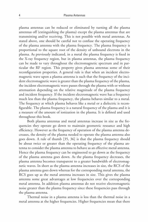
PlasmaAntennas
plasma antennas can be reduced or eliminated by turning all the plasma antennas off (extinguishing the plasma) except the plasma antennas that are transmitting and/or receiving. This is not possible with metal antennas. As stated above, one should be careful not to confuse the operating frequency of the plasma antenna with the plasma frequency. The plasma frequency is proportional to the square root of the density of unbound electrons in the plasma. As previously indicated, in a metal the plasma frequency is fixed in the X-ray frequency region, but in plasma antennas, the plasma frequency can be made to vary throughout the electromagnetic spectrum and in par-ticular the RF region. This property gives plasma antennas some of their reconfiguration properties. A general rule is that when an incident electro-magnetic wave upon a plasma antenna is such that the frequency of the inci-dent electromagnetic wave is greater than the plasma frequency of the plasma, the incident electromagnetic wave passes through the plasma with or without attenuation depending on the relative magnitude of the plasma frequency and incident frequency. If the incident electromagnetic wave has a frequency much less than the plasma frequency, the plasma behaves similar to a metal. The frequency at which plasma behaves like a metal or a dielectric is recon-figurable. The plasma frequency is a natural frequency of the plasma and it is a measure of the amount of ionization in the plasma. It is defined and used throughout this book.
Both plasma antennas and metal antennas increase in size as the fre-quencies they operate go down to maintain geometric resoance and high efficiency. However as the frequency of operation of the plasma antenna de-creases, the density of the plasma needed to operate the plasma antenna also goes down. A rule of thumb [35, 36] is that the plasma frequency should be about twice or greater than the operating frequency of the plasma an-tenna to consider the plasma antenna to behave as an effective metal antenna. Hence the plasma frequency can be engineered to go down as the frequency of the plasma antenna goes down. As the plasma frequency decreases, the plasma antenna becomes transparent to a greater bandwidth of electromag-netic waves. In short as the plasma antenna increases in size, the RCS of the plasma antenna goes down whereas for the corresponding metal antenna, the RCS goes up as the metal antenna increases in size. This gives the plasma antenna some great advantages at low frequencies over the corresponding metal antenna. In addition plasma antennas do not receive electromagnetic noise greater than the plasma frequency since these frequencies pass through the plasma antenna.
Thermal noise in a plasma antenna is less than the thermal noise in a metal antenna at the higher frequencies. Higher frequencies mean that there

Introduction
is a point in the RF spectrum in which the thermal noise of plasma antennas is equal to the thermal noise of metal antennas. At higher frequencies than this point, the plasma antenna thermal noise decreases drastically compared to a metal antenna. Below this point the thermal noise of the plasma an-tenna is greater than a metal antenna. For a flourescent tube that is used as a plasma antenna, the point where the thermal noise of the plasma antenna is equal to the metal antenna is about 1.27 GHz. This point can be decreased in frequency by decreasing the plasma pressure. The plasma in the plasma antennas are inert gases that operate at energies and frequencies in which Ramsauer–Townsend effects apply.
Ramsauer–Townsend effects mean that the electrons in the plasma dif-fract around the ions and neutral atoms in the plasma. This means that the collision rate of the unbound electrons in the plasma with ions and neutral atoms is small and much smaller than in a metal. This phenomenon contrib-utes to the lower thermal noise that plasma antennas have over corresponding metal antennas.
Satellite plasma antennas benefit from the lower thermal noise at the frequencies they operate. Ground-based satellite antennas point at space where the thermal noise is about 5K. A low thermal noise, a high data rate satellite plasma antenna system is possible with low noise plasma feeds and a low noise receiver. Satellite plasma antennas can operate in the reflective or refractive mode. Satellite plasma antennas need not be parabolic but can be flat or conformal and effectively parabolic. Electromagnetic waves reflecting off of a bank of plasma tubes get phase shifted as a function of the plasma density in the tube. This becomes an effective phased array except that the phase shifts are determined by the plasma density. If the plasma density in the tubes is computer controlled, the reflected beam can be steered or focused even when the bank of tubes is flat or conformal. In the refractive mode, the refraction of electromagnetic waves depends upon the density of the plasma. In the refractive mode, steering and focusing can be computer controlled even when the bank of tubes is flat or a conformal shape. For two-dimensional steering and/or focusing, two banks of plasma tubes are needed. Feed horns and receivers can be put behind satellite plasma anten-nas operating in the refractive mode. This eliminates the problem of the blind spot and feed losses caused by the feed horn and receiver in front of a metal satellite antenna.
The above phenomena of using a bank of plasma tubes to focus elec-tromagnetic waves is also known as a convergent plasma lens. A conver-gent plasma lens can focus electromagnetic waves to decrease beamwidths, increase directivity, and increase antenna range. A divergent plasma lens can

PlasmaAntennas
also be created. Both convergent and divergent plasma lenses lead to recon-figurable beamwidths.
High powered plasma antennas have been developed which transmit 2 MW and more in the pulsed mode.
Pulsing techniques instead of applying continuous energy were devel-oped to increase the plasma density and decrease the amount of energy to maintain the plasma. The early techniques used spark gap techniques for pulsing. This technique produced some EMI noise, which was suppressed using circuit techniques. Techniques that did not use spark gap techniques to produce pulsing did not produce EMI noise. Continuous energy applications to ionize and maintain ionization did not produce EMI noise.
No infrared signature of the plasma antenna when the plasma is con-tained in glass tubes has been observed. This is partly due to infrared radia-tion not penetrating glass and that the plasma in a plasma antenna is not a blackbody radiator.
Related to plasma antennas, plasma frequency selective surfaces, plasma waveguides, and plasma coaxial cables have been developed. Unlike metal fre-quency selective surfaces, plasma frequency selective surfaces have the prop-erties of reconfigurable filtering of electromagnetic waves. This could have tremendous advantages to radome design. Plasma frequency selective surfaces can be reconfigured by varying the plasma density, varying the shape of the elements, or tuning any number of the plasma FSS elements on or off. Plasma wave guides and plasma coaxial cables can be stealth-like plasma antennas, they can operate at low frequencies, and be invisible at high frequencies. Plasma waveguides and coaxial cables can be feeds for plasma antennas. Plasma feeds as well as the plasma antennas have reconfigurable impedances. If the imped-ance of the plasma antenna is changed, the impedance of the plasma feeds can be changed to maintain impedance matching.
In the history of antennas, it has been difficult to develop low frequency directional and electronically steerable antennas that fit on land vehicles and air-craft. Low frequency means the wavelength is on the order or larger than the ve-hicle. With plasma antennas this is possible with multipole expansions of clusters of plasma antennas that are all within a wavelength of each other. This depends on the ability of turning plasma antennas on or off (extinguishing the plasma) to create reconfigurable multipoles of plasma antennas that can be rotated in time creating directional and steerable antenna beams. This is not possible with metal antennas because the metal cannot be turned on and off.
In this book, plasma antennas were fed by capacitive sleeves placed around the plasma tubes. Plasma antennas can also be fed inductively.

Introduction
For research purposes, fluorescent and neon tubes have been used to build plasma antennas since they are inexpensive. The fact that you can use COTS tubes as plasma antennas gives the plasma antenna an advantage. COTS tubes may be all that is needed for many applications or deployments. This makes the technology less costly and more appealing. In addition fluo-rescent and neon tubes are not trivial technologies. The proliferation and commonalty of fluorescent and neon tubes may make them seem like unso-phisticated technologies. However, they are sophisticated.
Plasma antennas have been housed in a synthetic foam called SynFoam. When this synthetic foam hardens it makes very strong and lightweight tubes that can be used as plasma tubes to make plasma antennas. These rugged tubes can be readily manufactured.
SynFoam [39] has been tested to have an index of refraction close to one and hence is very transparent to electromagnetic waves. SynFoam is very heat resistant. The ruggedized smart plasma antenna shown in Figure 7.13 of Chapter 7 uses SynFoam to house the plasma.
Gorilla glass by Corning [40] and Lexan glass [41] tubes are also op-tions for housing plasmas.
Plasma antennas can also be miniaturized and contained in commer-cially available cold cathode tubes [42] used for liquid crystal displays. Ball and socket glass tubes [43] inserted inside plastic tubes can be used to make flexible plasma antennas that can be shaped in various forms.
In summary, the plasma of plasma antennas can be housed in Synfoam, miniaturized cold cathode tubes, ball and socket glass tubes, Lexan glass, and Gorilla glass by Corning. These materials can readily be manufactured. References [44–72] will also give readers with an additional understanding of plasma antennas, plasma waveguides, plasma frequency selective surfaces, and plasma filters.
References
[1] Krall, N., and A. Trivelpiece, PrincipalsofPlasmaPhysics, McGraw-Hill Inc., 1973.
[2] Chen, F., IntroductiontoPlasmaPhysicsandControlledFusion,Springer, 2006.
[3] Jackson, J.D., ClassicalElectrodynamics, New York: John Wiley & Sons, 1998.
[4] Ulaby, F.T., FundamentalsofAppliedElectromagnetics, Prentice Hall, 1999.
[5] Feynman, R., R. Leighton, and M. Sands, TheFeynmanLecturesonPhysics, Vol. 1–3, Pearson Addison Wesley, 2006.
PlasmaAntennas
[6] Kraus, J., and R. Marhefka, AntennasforAllApplications,ThirdEdition, McGraw-Hill, 2002.
[7] Balanis, C., AntennaTheory,SecondEdition, John Wiley & Sons, 1997.
[8] Landau, L.D., and E.M. Lifshitz, FluidMechanics,SecondEdition, Vol. 6, Reed Educa-tional & Professional Publishing Ltd., 2000.
[9] http://www.ionizedgasantennas.com.
[10] http://www.drtedanderson.com.
[11] http://ieeexplore.ieee.org/Xplore/login.jsp?url=http%3A%2F%2Fieeexplore.ieee.org%2Fiel5%2F4345408%2F4345409%2F04345600.pdf%3Farnumber%3D4345600&authDecision=-203.
[12] http://www.haleakala-research.com/uploads/operatingplasmaantenna.pdf.
[13] Anderson, T., “Multiple Tube Plasma Antenna,” U.S. Patent 5,963,169, issued Octo-ber 5, 1999.
[14] Anderson, T., and I. Alexeff, “Reconfigurable Scanner and RFID,” Application Serial Number 11/879,725. Filed 7/18/2007.
[15] Anderson, T., “Configurable Arrays for Steerable Antennas and Wireless Network In-corporating the Steerable Antennas.” U.S. Patent 7,342,549, issued March 11, 2008.
[16] Anderson, T., “Reconfigurable Scanner and RFID System Using the Scanner”. U.S. Patent 6,922,173, issued July 26, 2005.
[17] Anderson, T., “Configurable Arrays for Steerable Antennas and Wireless Network In-corporating the Steerable Antennas,” U.S. patent 6,870,517, issued March 22, 2005.
[18] Anderson, T., and I. Alexeff, “Theory and Experiments of Plasma Antenna Radia-tion Emitted Through Plasma Apertures or Windows with Suppressed Back and Side Lobes,” InternationalConferenceonPlasmaScience, 2002.
[19] Anderson, T., “Storage And Release Of Electromagnetic Waves by Plasma Antennas and Waveguides,” 33rdAIAAPlasmadynamicsandLasersConference, 2002.
[20] Anderson, T., and I. Alexeff, “Plasma Frequency Selective Surfaces,” IEEETransactionsonPlasmaScience, Vol. 35, No. 2, April 2007, p. 407.
[21] Munk, B.A., FrequencySelectiveSurfaces, Wiley Interscience, 2000.
[22] Feynman, R., R. Leighton, and M. Sand, The Feynman Lectures on Physics. Vol. 2, Chapter 6, 1966.
[23] Balanis, C., AntennaTheory,SecondEdition, John Wiley & Sons, pp. 785–835.
[24] Pierce, A.D., Acoustics:AnIntroductiontoItsPhysicalPrinciplesandApplications, Sec-tion 4-4 Dipoles and Quadrupoles, 1989.
[25] Linardakis, P., G. Borg, and N. Martin, “Plasma-Based Lens for Microwave Beam Steering,” ElectronicsLetters, Vol. 42, No. 8, April 13, 2006, pp. 444–446.
Introduction
[26] Reif, F., Fundamentals of Statistical and Thermal Physics, McGraw-Hill, 1965, pp. 585–589.
[27] Anderson, T., “Electromagnetic Noise from Frequency Driven and Transient Plas-mas,” IEEEInternationalSymposiumonElectromagneticCompatibility,SymposiumRe-cord, Vol. 1, Minneapolis, MN, August 19–23, 2002.
[28] Anderson., T., “Control of Electromagnetic Interference from Arc and Electron Beam Welding by Controlling the Physical Parameters in Arc or Electron Beam: Theoretical Model,” 2000IEEESymposiumRecord, Vol. 2, pp. 695–698.
[29] Pierce, A.D., Acoustics:AnIntroductiontoItsPhysicalPrinciplesandApplications, Sec-tion 2-10, published by the American Physical Society through the American Institute for Physics, 1989.
[30] Manheimer, W., “Plasma Reflectors for Electronic Beam Steering in Radar Systems,” IEEETransactionsonPlasmaScience, Vol. 19, No. 6, December 1993, p. 1228.
[31] Mathew, J., et al., “Electronically Steerable Plasma Mirror for Radar Applications,” IEEE InternationalRadarConference, June 1995, p. 742.
[32] Moisan, M., A. Shivarova, and A.W. Trivelpiece, “Surface Waves on a Plasma Col-umn”, Phys.Plasmas, Vol. 20, 1982.
[33] Borg, G., et al., “Plasmas as Antennas: Theory, Experiment, and Applications,”Physicsof Plasmas, Vol. 7, No. 5, May 2000, p. 2198.
[34] Borg, G.G., et al., “Application of plasma columns to radiofrequency antennas,” Appl.Phys.Lett. Vol. 74, 1999.
[35] Alexeff, I , and T. Anderson., “Experimental and Theoretical Results with Plasma An-tennas,” IEEETransactionsonPlasmaScience, Vol. 34, No. 2, April 2006.
[36] Alexeff, I., and T. Anderson,“Recent Results of Plasma Antennas,” PhysicsofPlasmas, Vol. 15, 2008.
[37] http://www.aps.org/meetings/unit/dpp/vpr2007/upload/anderson.pdf.
[38] Jenn, D.C., “Plasma Antennas: Survey of Techniques and the Current State of the Art,” Naval Postgraduate School, September 29, 2003, http://faculty.nps.edu/jenn/pubs/PlasmaReportFinal.pdf.
[39] http://www.udccorp.com/products/synfoamsyntacticfoam.html.
[40] http://www.corninggorillaglass.com/.
[41] http://en.wikipedia.org/wiki/Lexan.
[42] http://www.jkllamps.com/files/BF20125-28B.pdf.
[43] http://en.wikipedia.org/wiki/Ground_glass_joint.
[44] Anderson, T., Plasma Devices For Steering and Focusing Antenna Beams; patent ap-plication number 20110025565; Filed July 22, 2010.

0 PlasmaAntennas
[45] Hambling, D., ScientistsControlPlasmaforPracticalApplications; Popular Mechanics; July 2010; page 18; http://www.popularmechanics.com/technology/engineering/news/scientists-control-plasma-for-practical-applications.
[46] Ashley, S., Aerial Stealth, Scientific American, February 2008 issue, page 22, “http://www.scientificamerican.com/article.cfm?id=aerial-stealth”.
[47] http://www.aps.org/meetings/unit/dpp/vpr2007/upload/anderson.pdf.
[48] http://www.msnbc.msn.com/id/22113395/ns/technology_and_science-innovation/t/new-radio-antenna-made-star-material/.
[49] http://www.livescience.com/2068-radio-antenna-plasma.html.
[50] http://pop.aip.org/phpaen/v15/i5/p057104_s1?view=fulltext&bypassSSO=1.
[51] http://ieeexplore.ieee.org/Xplore/login.jsp?url=http%3A%2F%2Fieeexplore.ieee.org%2Fiel5%2F27%2F33960%2F01621284.pdf%3Farnumber%3D1621284&authDecision=-203.
[52] http://www.scribd.com/doc/45554477/Operating-Plasma-Antenna, www.scribd.com/doc/45554477/Operating-Plasma-Antenna.
[53] ieeexplore.ieee.org/iel5/27/33960/01621284.pdf?arnumber=1621284.
[54] http://www.mendeley.com/research/experimental-theoretical-results-plasma-antennas/
[55] http://www.mdatechnology.net/update.aspx?id=a4112.
[56] http://www.afsbirsttr.com/Library/Documents/Innovation-092908-Haleakala-AF05-041.pdf.
[57] http://www.antennasonline.com/AST-Conf11/ast11_program.php#ha.
[58] Anderson, T., U.S. Pat. No. 6,806,833: Confined Plasma Resonance Antenna andPlasmaResonanceAntennaArray, issued Oct. 19, 2004 with inventor Theodore R. Anderson.
[59] Anderson, T., U.S. Pat. No. 6,674,970: PlasmaAntennawithTwo-FluidIonizationCurrent, issued Jan. 6, 2004.
[60] Anderson, T., U.S. Pat. No. 6,657,594: PlasmaAntennaSystemandMethod, issued Dec. 2, 2003.
[61] Anderson, T., Aiksnoras, R., U.S. Pat. No. 6,650,297: LaserDrivenPlasmaAntennaUtilizingLaserModifiedMaxwellianRelaxation, issued Nov. 18, 2003.
[62] Anderson, T., U.S. Pat. No. 6,169,520: PlasmaAntennawithCurrentsGeneratedbyOpposedPhotonBeams, issued Jan. 2, 2001.
[63] Anderson, T., Aiksnoras, R., U.S. Pat. No. 6,087,993: PlasmaAntennawithElectro-OpticalModulator, issued July 11, 2000.
[64] Anderson, T., U.S. Pat. No. 6,046,705: StandingWavePlasmaAntennawithPlasmaReflector, issued April 4, 2000.
Introduction
[65] Anderson, T., U.S. Pat. No. 6,118,407: HorizontalPlasmaAntennausingPlasmaDriftCurrents, issued Sept. 12, 2000.
[66] Anderson, T., U.S. Pat. No. 6,087,992: AcousticallyDrivenPlasmaAntenna. issued July 11, 2000.
[67] Anderson, T., and I. Alexeff, Reconfigurable Electromagnetic Waveguide, U.S. Patent No. 6,624,719, issued September 23, 2003.
[68] Anderson, T., and I. Alexeff, ReconfigurableElectromagneticPlasmaWaveguideUsedasaPhaseShifterandaHornAntenna, U.S. Patent No. 6,812,895, issued November 2, 2004.
[69] Norris, E., Anderson, T., Alexeff, I. ReconfigurablePlasmaAntenna, U.S. Pat. No. HY-PERLINK “http://patft.uspto.gov/netacgi/nph-Parser?Sect2=PTO1&Sect2=HITOFF&p=1&u=%2Fnetahtml%2FPTO%2Fsearch-bool.html&r=1&f=G&l=50&d=PALL&RefSrch=yes&Query=PN%2F6369763” \l “h0#h0” HYPERLINK “http://patft.uspto.gov/netacgi/nph-Parser?Sect2=PTO1&Sect2=HITOFF&p=1&u=%2Fnetahtml%2FPTO%2Fsearch-bool.html&r=1&f=G&l=50&d=PALL&RefSrch=yes&Query=PN%2F6369763” \l “h2#h2” 6,369,763, issued April 9, 2002.
[70] Anderson, T., Alexeff, I., Antenna Having Reconfigurable Length, U.S. Pat. No 6,710,746, issued March 23, 2004.
[71] Alexeff, I., Anderson, T., Norris, E., ReconfigurablePlasmaAntennas, U.S. Pat. No 6,876,330, issued April 5, 2005.
[72] http://www.pdf-archive.com/2011/03/14/lockheedmartin/lockheedmartin.pdf.

13
2Plasma Physics for Plasma Antennas
2.1 Mathematical Models of Plasma Physics
Readers can broaden their understanding of plasma physics by reading Krall [1] and Chen [2]. The author particularly recommends the Feynman lectures [3] for an understanding of basic plasma physics. The kinetic description of plasma can be made by a many body description governed by the Liouville equation. From the Liouville equation, the Boltzmann transport equation and the collisionless Boltzmann equation or the Vlasov equation can be de-rived to give a kinetic description of the plasma.
Plasma antenna characteristics are much better described by the fluid model. Macroscopic variables of the plasma are given in the fluid model. These macroscopic variables include density, particle flux, velocity, current density, heat flux, and the pressure tensor. Similar to a description given by the Navier-Stokes and continuity equations of classic fluid dynamics, the fluid model of the plasma is given in terms of momentum equations, conti-nuity equations, and Maxwell’s equations.
The two-fluid model of plasma physics describes the electrons and ions as conducting fluids that are couples through momentum transfer collisions and Maxwell’s equations. The set of equations involved include continuity, momentum, and Maxwell’s equations. In the two-fluid equations ions and electrons are indentified as separate species.

14 PlasmaAntennas
The one-fluid model of plasma physics combines the density and veloc-ity of the electrons and ions. The variables include total mass density, center of mass velocity, electric field, and charged density.
The magnetohydrodynamic (MHD) equations of one-fluid plasma physics are obtained by using long spatial scale phenomena, low frequencies, and collisions sufficiently frequent that the plasma is isotropic at all times.
A plasma is very rich in wave phenomena, and the fluid models can describe much of it. The fluid equations can be linearized in the wave phe-nomena assuming small amplitude waves. Once perturbed harmonic wave quantities are substituted into the fluid and Maxwell’s equations, the result-ing equations are linearized. From the resulting linearized equations, various plasma wave phenomena can be solved.
One solution of the linearized equations corresponds to electromag-netic oscillations at the plasma frequency. These oscillations are called plasma oscillations, Langmuir oscillations, and space charge waves. These oscillations are dispersionless in a cold plasma. They have a group velocity of zero and do not propagate in a cold plasma. The plasma oscillations have a nonzero phase velocity.
2.2 Man-Made Plasmas and Some Applications
Plasmas can be generated by the application of electric and/or magnetic fields, RF heating, and laser excitation. The type of power source used to generate the plasma can be DC, RF, laser, and microwave. The pressure at which plas-mas operate can be vacuum pressure (< 10 mTorr or 1 Pa), moderate pressure (~1 Torr or 100 Pa), or atmospheric pressure (760 Torr or 100 kPa). A plasma can be fully ionized or partially ionized. Using temperature descrip-tions of a plasma, a plasma can be thermal, in which case the electron and ion temperature are equal to each other and the gas temperature (Te = Tion = Tgas). A plasma can be nonthermal or “cold” plasma, in which case the elec-tron temperature is much greater than the ion temperature and the ion tem-perature is equal to the gas temperature(Te >> Tion = Tgas). A plasma can be characterized by the electrode configurations used to generate the plasma. The interaction of the plasma with a magnetic field can characterize a plasma in the following ways: Magnetized (both ion and electrons are trapped in Larmor orbits by the magnetic field); partially magnetized (the electrons but not the ions are trapped by the magnetic field); or nonmagnetized (the magnetic field is too weak to trap the particles in orbits but may generate Lorentz forces.). Vari-ous applications of plasmas besides antennas are fusion, magnetohydrodynmaic

PlasmaPhysicsforPlasmaAntennas 15
generators, populsion, and glow discharge plasmas that include fluorescent tubes. Glow discharge plasmas are nonthermal plasmas generated by the ap-plication of DC or low frequency RF (<100 kHz) electric field to a gas be-tween two metal electrodes. Capacitively coupled plasmas are similar to glow discharge plasmas, but generated with high-frequency RF electric fields, typi-cally 13.56 MHz differ from glow discharges in that the sheaths are much less intense. Microfabrication and integrated circuit manufacturing industries for plasma etching and plasma enhanced chemical vapor deposition use capaci-tively coupled plasmas. Inductively coupled plasmas have similar applications but the electrode consists of a coil wrapped around the discharge volume that inductively excites the plasma. RF heating of a plasma is done in some fusion designs. An arc discharge plasma is a high-power thermal discharge of very high temperature (~10,000 K). A corona discharge is a nonthermal discharge generated by the application of high voltage to sharp electrode tips and can be used in ozone generators and particle precipitators.
2.3 Basic Physics of Reflection and Transmission from a Plasma Slab Barrier
The reflection and transmission coefficients for electromagnetic waves im-pinging on a plasma rectangular slab are [4]:
−=
+p
p
k kR
k ko
o (2.1)
2
p
kT
k k=
+o
o (2.2)
where k0 is the wavenumber of the impinging electromagnetic wave, kp is the wavenumber of the electromagnetic wave in the plasma, c is the speed of light, and w is the frequency of the impinging electromagnetic wave.
2 2 2k cο ω= (2.3)
and
22 2 2
21p
pk cω
ωω
= −
(2.4)
16 PlasmaAntennas
and
=
24p
e
nemπω
(2.5)
n is the unbound electron density and a measure of the amount of ionization. e is the charge on the electron and me is the electron mass. Equation (2.5) is known as the plasma frequency. It is a natural frequency of the plasma and is a measure of the amount of ionization in a plasma. The reader should not confuse the plasma frequency with the operating frequency of a plasma an-tenna. In this case, the plasma frequency is in Gaussian units. See (5.1) for the conversion of the plasma frequency to mks units.
If the density of the plasma is high enough such that
<< pω ω (2.6)
then
= −1R (2.7)
and
= 0T (2.8)
Thus, the plasma reflects waves with a frequency below the plasma fre-quency with the same amplitude and phase as though the plasma were re-placed by a perfect conductor.
In the case, the incident frequency of the electromagnetic wave is much greater than plasma frequency as in the case of very low-density plasmas, the reflection coefficient, R, is zero, and the transmission coefficient, T, is 1.
>> pω ω (2.9)
= 0R (2.10)
and
=1T (2.11)
However, when the plasma density is in between these extremes, such that
≤ ppω ω (2.12)

PlasmaPhysicsforPlasmaAntennas 17
or
≥ pω ω (2.13)
Then there is a combination of absorption, reflection, and transmission.This phenomenon is dependent on the relative values of w and wp in-
dependent of the absolute values of w and wp. This can occur anywhere on the spectrum.
2.4 Experiments of Scattering Off of a Plasma Cylinder
A cylinder is a basic geometry of antennas and frequency selective surfaces (FSS) and experiments on scattering off of cylindrical plasmas can give valu-able information on the utility of plasma antennas and plasma FSS.
Tonks [5] studied plasma discharge columns and was the first to per-form experiments of scattering electromagnetic waves off of a plasma column at resonance. A summary of the Tonks’ experiment can be found in Krall and Trivelpiece [6]. A wave from a signal source is propagated into a wave-guide with dimensions corresponding to a cutoff wavelength of 10 cm. A thermionic-arc discharge column is situated at right angles to the incident waveguide electric field. Two direction couplers sample the amplitude of the incident wave and the amplitude of the reflected wave. The experiment con-sists of measuring the ratio of the scattered power reflected by the plasma to the power incident on the plasma as a function of the density of the plasma. The discharge column is a thermionic-arc discharge in mercury vapor at a pressure (10-3 Torr) such that the plasma electron density is proportional to the dc current in the discharge. The plasma is collisionless since the mean free path of plasma electrons is much greater than the diameter of the plasma columns.
The wavelength of the incident wave is much greater than the radius of the plasma column so thatthe electric field in the vicinity of the plasma column is nearly irrotational and the electric field can be derived from a scalar potential.
The electrical potential satisfies Laplace’s equation with no zvariation, both inside and outside the plasma.
The boundary conditions at a dielectric-vacuum interface are that the normal component of the displacement and tangential component of the electric field be continuous. These conditions are satisfied at the plasma-air boundary.

18 PlasmaAntennas
Satisfaction of the boundary conditions gives the potential inside the plasma in terms of the incident amplitude and frequency and it is shown that the field in the plasma becomes large (resonant) when the frequency is:
=
2pω
ω
(2.14)
where the 2 is characteristic of the cylindrical geometry and wp is the plasma frequency.
=
24 op
n em
πω
(2.15)
This is the main and largest resonance peak. Other and smaller scatter-ing peaks satisfy the Bohm-Gross dispersion relation given by:
2 2 23p
e
Tk
mκω ω= +
(2.16)
Since the plasma column is resonant at = 2pω ω , the electrons in the column oscillate in response to the driving electric field. This motion reradi-ates, or scatters, the incident field in cylindrical waves. Since the motion of the electrons in the plasma is largest at resonance, the scattered power will be a maximum at resonance.
It may be possible to harness these resonance effects to the advantage of plasma antennas over metal antennas.
2.5 Governing Plasma Fluid Equations for Applications to Plasma Antennas
The plasma charge and current densities are defined by:
( , ) [ ( , ) ( , )]r t e p r t n r tρ = − (2.17)
and
( , ) [ ( , ) ( , ) ( , ) ( , )]PJ r t e p r t V r t n r t V r t= −
(2.18)

PlasmaPhysicsforPlasmaAntennas 19
respectively. In (2.17) and (2.18), ( , )p r t and ( , )n r t refer to the volume number density of positive and negative charges, respectively, e is the elemen-tary unit of charge ( , )n r t (taken to be a positive number), and ( , )pV r t
and ( , )nV r t are the respective velocity fields associated with positive and negative
charges.Local charge imbalance gives rise to an electrostatic potential f, which
is determined by Poisson’s equation:
2 ( , ) 4 [ ( , )] ( , )r t p r t n r tφ π∇ = − − (2.19)
Note that the equations in this chapter are in cgs units.We assume a fixed degree of ionization of the plasma so that we can as-
sume each charge species to be locally conserved. This assumption gives rise to continuity equations connecting the charge and current densities of each charge species separately:
∂= −∇ ⋅
∂ p
pJt
ρ
(2.20)
and
∂ = −∇ ⋅∂
nnJ
tρ
(2.21)
where we have taken the following definitions for the individual charge and current densities:
= ( , ) ( , )p r t ep r tρ (2.22)
= ( , ) ( , ) ( , )p pJ r t eV r t p r t (2.23)
= − ( , ) ( , )n r t en r tρ (2.24)
= − ( , ) ( , ) ( , )nJ r t eV r t n r t (2.25)
In order to obtain a set of linear equations, we will consider small devia-tions from charge neutrality. We thus write:

20 PlasmaAntennas
= + ( , ) ( , )op r t p p r tδ (2.26)
= +( , ) ( , )on r t n n n tδ (2.27)
where for a neutral system no = po and we assume the terms dp and dn are small. Using (2.26) and (2.27), linearize the continuity equations as follows:
∂= − ∇ ⋅
∂ p
o pep Vt
ρ
(2.28)
∂ = + ∇ ⋅∂
no nen V
tρ
(2.29)
Lastly, changes in the velocity fields are governed by Newton’s equa-tions of motion:
( , ) ( , )
pp p
dV AM V e E r t r t
dt tγ φ
∂+ = + −∇ − ∂
(2.30)
for the positive charges and
( , ) ( , )n
n ndV A
M V e E r t r tdt t
γ φ ∂+ = + −∇ − ∂
(2.31)
for the negative charges. In (2.30) and (2.31) E is an externally applied electric
field, M is the mass of the positive species (typically ions), A is the magnetic vector potential, and m is the mass of the negative species (typically electrons). We have also included phenomenological damping terms characterized by the collision frequencies gp and gn, respectively, for the positive and negative species.
Now we derive the equation of motion for the current density by differ-entiating (2.18) and substituting (2.28), (2.29), (2.30), and (2.31), to give
2 ( ) ( )o op o p o n
pJ A ne E eV p V eV n V
t t M mφ
∂ ∂ = −∇ − + + − ∇ ⋅ − − ∇ ⋅ ∂ ∂
(2.32)

PlasmaPhysicsforPlasmaAntennas 21
Next we linearize by dropping the last two terms in (2.32). Another simplification occurs by noting that typically the ionic mass is much larger than the electron mass M >> m justifying the neglect of the p0/M term in (2.32). Physically this corresponds to the assumption that positive charge density is essentially uniform with the constant value po.
This completes the derivation of the fluid model. The following three linear equations must be solved simultaneously:
2
4pJ A
J Et t
ωγ φ
π ∂ ∂+ = −∇ − ∂ ∂
(2.33)
∂ = ∇ ⋅∂
J
tρ
(2.34)
∇ = −2 4φ πρ (2.35)
We have dropped the subscript on the collision frequency (gn ® g) and we have introduced the plasma frequency, which is again defined by:
=
24 op
n em
πω
(2.36)
which is the frequency of free plasma oscillations in the absence of an applied field (i.e., for the case
E = 0).
2.6 Incident Signal on a Cylindrical Plasma
The application of the plasma fluid equations to a cylindrical geometry is given next. An antenna signal represented as an incident field is assumed to be a plane wave polarized along the length of the plasma column. The field in (2.33) is simply given by
⊥= − ⋅
0ˆ( , ) cos( )E r t zE t k rω (2.37)
where ⊥k , the propagation vector, lies in the x-y plane. Assume that the plasma
exists in a transparent container consisting of a right circular cylinder of length L

22 PlasmaAntennas
aligned with the z-axis and radius a. We restrict attention to wavelengths 0 £ l £ L and we assume that a << L (in practice, we take a = L /6). With these assump-tions we can neglect the spatial dependence of the phase factor in (2.37) and we take
w= ˆ( , ) cos( )oE r t zE t (2.38)
2.7 Fourier Expansion of the Plasma Antenna Current Density
Equations (2.33), (2.34), and (2.35) can be combined to give a single equa-tion in terms of the plasma antenna current density
J , which can be solved
by Fourier transformation upon applying the appropriate boundary condi-tions. Physically the current density must vanish at the ends of the cylindrical container [i.e., J(z = 0; t) = J(z = L; t) = 0]. Therefore, we expand the current density in a Fourier sine series:
∞≡ = + ∑
1
ˆ( , ) ( , ) cos( ) sin( / )lJ r t J z t z t a l z Lω α π
(2.39)
By a simple manipulation of (2.34) and (2.35) and the substitution of (2.39), we have the following forms for ∇
φ and ∂ ∂
J t:
∞∇ = + ∑
1
4sin( ) sin( / )t l z L
πφ ω α πω
(2.40)
and
∞∂ = − +∂ ∑
1
ˆ sin( ) sin( / )J
z t l z Lt
ω ω α π
(2.41)
2.8 Plasma Antenna Poynting Vector
The intensity pattern of the plasma antenna is related to the time averaged Poynting vector. These quantities can be solved by calculating the potentials and fields in the far field.

PlasmaPhysicsforPlasmaAntennas 23
In the far-field approximation, the vector and scalar potentials are given by:
−′⋅′= ∫ ˆ( , ) ( , )
jkrjr r ke
A r t dr J r t erc
(2.42)
and
′⋅− ′= ∫ ˆ( , ) ( , ) jr r ke jkr
r t dr r t er
φ ρ
(2.43)
where the unit vector n points in the direction of the observation point ˆ /n r r= .At this point it is convenient to switch to complex exponentials for the
time dependence as well as the spatial dependence as indicated in (2.42) and (2.43). The conversion is made by the following two replacements:
− + −+ → ( )cos( ) jkr j t krt e e ω αω α (2.44)
and
− + −+ → − ( )sin( ) jkr j t krt e je ω αω α (2.45)
Upon substituting (2.17) and (2.39) into (2.42) and (2.43) and invok-ing (2.44) and (2.45), we obtain integrals for the vector and scalar potentials that can be evaluated in a closed form.
Once the plasma current and charge densities are obtained from the plasma fluid equations, the plasma antenna far field potentials can be solved for. When the potentials are calculated, the corresponding fields can be computed:
∂= ∇ −∂
1 AE
c tφ
(2.46)
where
∂∇ ⋅ + =∂
2 0c Atφ
(2.47)
and
= ∇×
B A (2.48)

24 PlasmaAntennas
In carrying out the differentiations in (2.46) and (2.48), we need only retain terms of order O(1/r) as these are the only ones that contribute in the far field. In particular, we find that lowest-order term arising from ∇
φ is of
order O(1/r2) and can thus be neglected.
= ×
*Re8c
P E Bπ
(2.49)
Once the time-averaged Poynting vector is obtained, the total radiated power, intensity pattern, and directivity of the plasma antenna can be com-puted.
The radial component of the time averaged Poynting vector:
* * *ˆRe Re8 8
rc c
P E B n E B E Bθ φ φ θp π = × ⋅ = −
(2.50)
where the last term on the right-hand side vanishes because Ef = 0. In keeping only the O(1/r) terms, we find /B A rφ θ≈ ∂ ∂ and (1/ ) /E c A tθ θ= − ∂ ∂ , where we use the relation ˆˆ ˆcos( ) sin( )z r θ θ θ= − to extract Aq from (2.42). The results are:
= ( , ) ( , )E r t B r tφ θ (2.51)
Substituting (2.51) into (2.50) and dividing by the incident flux,
= 2
8inc o
cP E
π (2.52)
yield the elastic differential scattering cross section:
=
Ω2el r
inc
d Pr
d Pσ
(2.53)
The integral yields the total elastic scattering cross section,
= Ω = Ω Ω ∫ ∫2 sinel elel
d dd d
d dσ σσ π θ θ
(2.54)

PlasmaPhysicsforPlasmaAntennas 25
2.9 Some Finite Element Solution Techniques for Plasma Antennas
A good conductor is characterized by the limit of large plasma frequency in comparison to the incident frequency. In the limit in which the plasma fre-quency vanishes, the plasma elements become completely transparent.
We turn now to the numerical solution (private communication with Esmaeil Farshi, 2007) of the problem of electromagnetic waves interacting with a partially to perfectly conducting cylinder of plasma of unit radius. The conductivity and the scattering properties of the cylinder are specified by the incident and plasma frequency. Solving the wave equation for the electric field,
∂∇ =∂
22
2 21 D
Ec t
(2.55)
subject to the boundary conditions that the tangential electric and magnetic fields must be continuous at the cylinder boundary. The interaction of the cylinder with an incident plane wave of a single frequency is considered.
In cylindrical geometry, the wave equation takes the form of Bessel’s equation:
∂ ∂ ∂+ + + =∂∂ ∂
2 22
2 2 21 1
0E E E
k Eερ ρρ ρ ϕ
(2.56)
where k = w/c and (r, j) are cylindrical polar coordinates.Some solutions of a finite element code to solve these equations are
presented. Figure 2.1 is a sketch of the problem at hand showing electro-magnetic waves interacting with a plasma cylinder of unit radius at right angles.
In the linear approximation, the induced charges and currents in the homogeneous plasma medium represent only the modification of wave prop-agation characteristics in a medium, as compared to the vacuum (i.e., the modification of the complex refractive index). In this case, the frequency and dispersion law of a propagating wave are strictly constant. In the presence of fluctuations in a medium, the situation is significantly altered. Thus, if the density of charged particles fluctuates, the induce current will also fluctuate,

26 PlasmaAntennas
that is, frequency and propagation orientation (scattering), or even the oc-currence of waves of another kind (transformation). In turn, new waves alter the plasma state, giving rise to induced currents associated with them, and they are also able to influence the propagation of the fundamental wave. The process of complex nonlinear interaction between fields and currents occurs in the plasma. We can deal separately with incident and scattered waves and assume the field of the incident wave and plasma parameters to be assigned.
Here we consider the scattering process of the electromagnetic waves in a plasma. This process is of self-important value from the point of view of studying wave propagation and absorption. For simplicity, we deal only with the isotropic plasma. Then we can assert that for the region of transparency of propagating waves w ñ wp, the plasma can be referred to as a purely electron gas, and the effects associated with the spatial dispersion of electric permittiv-ity can be neglected (i.e., a simple expression) and
2
2( ) 1pω
ε ωω
= −
(2.57)
can be used for dielectric permittivity. The barrier penetration of electric field versus w/wp will be calculated.
Figure 2.1 Cylinderoftheplasmaofaunitradius.

PlasmaPhysicsforPlasmaAntennas 27
For solutions of finite element code for various ratios of w/wp, the elec-tric field is plotted at various points within the plasma cylinder with radius of unity in Figures 2.2, 2.3, and 2.4. In all cases, the amplitude of the electric field is normalized with a maximum value of one. The reader can ignore the finite element code information around these figures.
Figure 2.2 Forthecaseofw=3wp.PlasmacylinderofunitradiusistransparenttoincidentEMwave.Theamplitudeoftheelectricfieldisnormalizedwithamaximumvalueofone.
Figure 2.3 Forthecaseofw=0.1wp.Strongdecayinsidetheplasmacylinderofunitra-dius.Theamplitudeoftheelectricfieldisnormalizedwithamaximumvalueofone.

28 PlasmaAntennas
2.9.1 Barrier Penetration
According to these results and results not shown, we plot a barrier penetra-tion of the electric field versus w/wp in Figure 2.5.
2.9.2 Calculation of Scaling Function
In the previous section the barrier penetration of the electric field versus w/wp was plotted. The results from the analysis of the scattering from a partially conducting cylinder can be obtained from the computed results for a per-fectly conducting cylinder. The difference between the partially conducting and perfectly conducting cylinders is the amplitudeof the current modes.
The reflectivity of a partially conducting cylinder can be determined from that of the perfectly conducting cylinder by scaling the reflectivity of the per-fectly conducting cylinder by some appropriately chosen scaling function. This conclusion follows from the fact that the reflectivity is directly proportional to the squared amplitude of the current distribution on the scattering elements.
We define the scaling function as:
= − 2( , ) 1.0p outS Eν ν (2.58)
Figure 2.4 Forthecaseofw=0.5wp.InthiscasethereissomeattenuationoftheEfieldamplitudeinaplasmacylinderofunitradius.Theamplitudeoftheelectricfieldisnormal-izedwithamaximumvalueofone.

PlasmaPhysicsforPlasmaAntennas 29
Figure 2.5 Barrierpenetrationofelectricfiledversusw/wp.
Figure 2.6 Scalingfunctionversusw /wpincylindricalgeometryforscatteringfromacyl-inderwithaunitradius.
30 PlasmaAntennas
where Eout is the total tangential electric field evaluated just outside of the cylinder. Clearly, from the results of the previous section, the scaling function takes on the values:
≤ ≤0.0 ( , ) 1.0pS ν ν (2.59)
for the fixed incident frequency n as the plasma frequency takes on the values:
≤ ≤ ∞0.0 pν (2.60)
The plot of scaling function versus w/wp has been calculated. This func-tion was obtained from the solution of the problem of scattering from a par-tially conducting, infinitely long cylinder with a unit radius using a finite element code. Then, according to these results, we plot the scaling function of the electric field (Figure 2.6). The scaling function is also used in Section 8.2.2.
References
[1] Krall, N., and A. Trivelpiece, PrinciplesofPlasmaPhysics, McGraw-Hill Inc., 1973.
[2] Chen, F. F., Introduction toPlasmaPhysicsandControlledFusion, Volume1, Second Edition, Springer, 1984.
[3] Feynman, R., R. Leighton, and M. Sands, TheFeynmanLectures onPhysics, Com-memorative Issue, Three Volume Set, Addison-Wesley, 1989.
[4] Krall, N., and A. Trivelpiece, Principles ofPlasmaPhysics, McGraw-Hill Inc., 1973, Section 4.5.1.
[5] Tonks, L., “The High Frequency Behavior of a Plasma,” Phys.Rev. Vol. 37, 1931, p. 1458.
[6] Krall, N., and A. Trivelpiece,Principles ofPlasmaPhysics, McGraw-Hill Inc., 1973, pp. 157–67.

31
3Fundamental Plasma Antenna Theory
3.1 Net Radiated Power from a Center-Fed Dipole Plasma Antenna
In the case of plasma antennas, plasma fluid models [1, 2] can be used to calculate plasma antenna characteristics. For example, we proceed with the derivation of net radiated power from a center-fed dipole plasma antenna with a triangular current to obtain an analytical solution. For simplicity, the equations are linearized and one dimension is considered with the plasma antenna dipole antenna oriented along the z-axis.
The momentum equation for electron motion in the plasma is:
( )j td
m v q Eedt
ωυ υ φ + = − −∇
(3.1)
where m is the mass of the electron, u is the electron velocity in the fluid model, n is the collision rate, e is the charge on the electron, E is the electric field, w is the applied frequency in radians per second, and f is the electric potential.
The continuity equation for electrons in the plasma is:
0 0
nn
t zυ∂ ∂+ =
∂ ∂ (3.2)
where n is the perturbed electron density and no is the background plasma density.

32 PlasmaAntennas
Combining the momentum equation with the continuity equation yields:
20
2( )
jn q En
v j z z
φω ω
∂ ∂= − − ∂ ∂ (3.3)
Gauss’s law is given as:
2
2
qn
z
φε
∂ =∂
(3.4)
The dielectric constant for the plasma is defined as:
2
1( )
p
jv
ωε
ω ω= −
− (3.5)
where
2
po
nqm
ωε
=
(3.6)
is the plasma frequency.Assuming the plasma antenna is a center fed dipole antenna with a
triangular current distribution as given in Balanis [3] and substituting (3.4), (3.5), and (3.6) into (3.3), and integrating over the length of the antenna, we obtain for the dipole moment of the plasma antenna:
20 0
22 [ ( ) ]p
q n E dp a
m jvω ω ω=
+ − (3.7)
where a is the cross-sectional area of the plasma antenna and d is the length of the plasma antenna.
The total radiated power is then given by
2 22
012rad
kP p
cω
πε=
(3.8)
where k is the wavenumber.

FundamentalPlasmaAntennaTheory 33
Substituting (3.7) into (3.8) yields:
2 202 4
2 2 2 2 2( )
( ) ( )48 [( ) ]
orad p
p
a EP kd
cε ωω
π ω ω ν ω
= − + (3.9)
In (3.9) we see that the net radiated power for a plasma antenna is uniquely a function of the plasma frequency and collision rates.
3.2 Reconfigurable Impedance of a Plasma Antenna
Beginning with the z-component of magnetic vector potential satisfying the Helmholtz equation in the plasma:
22 2 2 2
2 ( ) ( ) ( ) ( ) 0z z zd d
r A kr r A kr k r A krdrdr
ν ν νn+ + − =
(3.10)
We obtain the magnetic field H by taking the curl of the magnetic vec-tor potential:
r z
r r k
H xAr z
A rA A
φ
φφ
∂ ∂ ∂= ∇ =∂ ∂ ∂
(3.11)
zAH
r∂= −∂
(3.12)
and
z zE j Aωµ= − (3.13)
In cylindrical coordinates, we obtain the magnetic and electric fields. We can then obtain the current and voltage across the antenna. By taking the ratio of the voltage to the current, we obtain the impedance of the plasma antenna. The vector equation satisfies the Helmholtz equation in cylindrical coordinates. The solutions are in terms of Bessel functions. The arguments

34 PlasmaAntennas
of the Bessel functions are imaginary for frequencies less than the plasma fre-quency and real for frequencies greater than the plasma frequency. The wave number inside the plasma is:
2 2
0 2 21 1p pk k jkο
ω ωω ω
= − = − −
(3.14)
The vector potential satisfies Bessel’s equation and has the solution
0( )zvA J jkυ γ= (3.15)
where
0k jk γ= − (3.16)
and
2
2 1pω
γω
= −
(3.17)
pω ω< (3.18)
The impedance becomes:
0 022 0 1 0
( ) ( )( ) ( )
z
z
j lA kr j lI k rVZ
A krI a k I k rar
ωµ ωµ γπ γ γπ
−= = =∂
∂
(3.19)
By varying the plasma density, we can vary the g and hence reconfigure the impedance between the plasma antenna and connecting lines or feeds and/or free space.
3.3 Thermal Noise in Plasma Antennas
See Anderson [4–6] for previous derivations on thermal noise. The correla-tion for the thermal noise voltage V(t) is given as:
20( ) ( ) ( ) ( / )i i i iR V t V t Vτ τ τ τ= + = −
(3.20)
FundamentalPlasmaAntennaTheory 35
Assume that the stochastic nature of plasma thermal noise is Poisson distributed. Using the Wiener-Khintchine theorem [7,8], we obtain the power spectral density of plasma noise.
0
2
0
( ) 4 ( )cos(2 )
4 exp( )cos(2 )ii
H f R f d
V v f d
τ π τ τ
τ π τ λ
∞
∞
=
= −
∫
∑∫
(3.21)
where R is the resistance in the plasma and e is the charge of the electron.The voltage fluctuation V is related to the electron velocity fluctuation
u as follows:
i i
eV R u
l=
(3.22)
Hence, the thermal noise power spectral density becomes:
22
0
Re( ) 4 exp cos( )H f u d
lτ ωτ τ
τ− = ∫
02 2
0
22
2
Re4
1
1/Re4
1 ( / )
ul
ul
τω τ
νω ν
= +
= +
(3.23)
where n is the collision frequency. Using the relationship from kinetic theory:
21 12 2
m u kT=
(3.24)

36 PlasmaAntennas
and the conductivity relationship:
2nem
σν
=
(3.25)
Substituting these quantities into the power spectral density for the plasma noise yields:
2
2
( ) 4
1plasma
RH f kT
ων
=+
(3.26)
For a solid current carrying metal:
( ) 4metalH f kTR= (3.27)
Hence, under certain conditions (see Chapter 12), the thermal noise of the plasma antenna is less than that of a corresponding metal antenna. The thermal noise derivation is more rigorously derived in Chapter 12.
References
[1] Krall, N., and A. Trivelpiece, PrinciplesofPlasmaPhysics, New York: McGraw-Hill, 1973, pp. 84–98.
[2] Chen, F., IntroductiontoPlasmaPhysicsandControlledFusion, Volume1, 2nd ed., New York: Plenum Press, 1984, pp. 53–78.
[3] Balanis, C., AntennaTheory, 2nd ed., 1997, New York: John Wiley & Sons, , p. 143.
[4] Anderson, T., “Electromagnetic Noise from Frequency Driven and Transient Plas-mas,” IEEE International Symposium on Electromagnetic Compatibility, Symposium Record, Vol. 1, Minneapolis, MN, August 19–23, 2002.
[5] Anderson, T., “Control of Electromagnetic Interference from Arc and Electron Beam Welding by Controlling the Physical Parameters in Arc or Electron Beam: Theoretical Model,” 2000 IEEE Symposium Record, Vol. 2, pp. 695–698.
[6] http://www.mrc.uidaho.edu/~atkinson/Huygens/PlasmaSheath/01032529.pdf.
[7] Reif, F., Fundamentals of Statistical and Thermal Physics, 1965, McGraw-Hill, pp. 587–589, 585–587.
[8] Pierce, A. D., “Acoustics: An Introduction to Its Physical Principles and Applications”, Acoustical Society of America, 1989, pp. 85–88.

37
4Building a Basic Plasma Antenna
4.1 Introduction
A simple plasma antenna can be built to demonstrate basic operation or as a class project [private communication with Fred Dyer, 2011]. Fortunately, ordinary fluorescent bulbs are an abundant and inexpensive source for the plasma element of an easily assembled plasma antenna. They are available in many sizes and shapes that are appropriate for various frequencies and appli-cations. Probably the most useful fluorescent bulbs are ones with a U shape that have electrode ends which can be placed inside a metal enclosure with only the glass tube exposed as an antenna (see Figure 4.1).
4.2 Electrical Safety Warning
Anyone trying to build a plasma antenna according to the methods in this chapter should consult a licensed electrical safety expert before proceeding. After consulting a licensed electrical safety expert, proceed as follows. Use a three-wire grounded power cord and securely attach the green ground wire to the metal enclosure. Install an appropriately sized fuse or circuit breaker to pro-tect from short circuits or overloads. Always unplug the unit before modifying or working inside. A battery-operated plasma antenna also contains potentially lethal high voltages. Several hundred volts are required to start a fluorescent lamp. Disconnect the battery and discharge capacitors before working inside.

38 PlasmaAntennas
4.3 Building a Basic Plasma Antenna: Design I
The plasma antenna shown in Figure 4.1 operates as a receiver for the stan-dard 88–108-MHz FM radio band. The large aluminum box is used as a base for the fluorescent lamp, to house the ballast and variable voltage trans-former, and as an RF shield to ensure that only the plasma inside the tube is acting as an antenna. A standard magnetic ballast appropriate for the tube is used, with a Variac variable voltage transformer controlling the input voltage to the ballast. Once the lamp is started with full 115 VAC input, the Variac can be used to lower ballast power voltage and therefore lower average current in the fluorescent bulb.
Plasma inside the fluorescent lamp acts as an antenna in exactly the same way as if it were a wire of the same shape. Note the small RF coupling box enveloping the lamp (Figure 4.1). This box has a BNC connector and coaxial cable connecting to a box (see the right side of Figure 4.1) containing the FM radio. RF coupling to the plasma column is through a metal sleeve surrounding a short length of the tube (see Figure 4.2). This provides capaci-
Figure 4.1 PlasmaantennausingastandardU-shapefluorescentlampandballast.Avari-ablevoltagetransformer(Variac)controlsplasmacurrentanddensity.AnFMreceiverisintheboxontherightwithacoaxialcableconnectedtoacapaci-tivecouplersurroundingthefluorescentlamp(ontheleftsideofthelamp).

BuildingaBasicPlasmaAntenna 39
tive coupling for the FM signal from the plasma column inside the tube to the coaxial cable then to the FM receiver.
To test the plasma antenna, first turn on the fluorescent lamp with the Variac adjusted to 115-V AC. Next turn on the FM radio and tune in to any FM radio station. Turning the lamp off deactivates the antenna and the FM station is no longer heard, only static. The current in the fluorescent lamp (and therefore the plasma density) can be lowered by reducing voltage on the Variac. As the current (plasma density) is slowly lowered, a point will be noted when the FM radio station reception disappears into static. This threshold current will be low compared to the normal operating current of the lamp, and the light from the tube will dim considerably.
The plasma antenna described here uses a standard magnetic ballast, but an electronic ballast (also standard for the particular lamp) will work equally well. These ballasts use AC voltage and current to run the lamp, generating electrical noise that potentially will cause RF interference with the
Captivecouplingsleeve
BNC connector
Metal boxfor shielding
Fluorescent bulb
Figure 4.2 Plasmacapacitivesleevecouplingasanantennafeed.Inductivecouplingcanalsobeused.

40 PlasmaAntennas
received signal. This is why an FM radio is used, which is quite immune to the AM electrical noise caused by the ballast. A similar AM antenna can be built if the standard fluorescent ballast is replaced with a constant current DC power supply. Without noise from a ballast, the standard 500–1,600-kHz AM stations can be easily received. Since the AM band is much lower in fre-quency than the FM band, a much lower corresponding current (and plasma density) is required. A simple DC supply can be made with a high voltage power supply connected to the fluorescent lamp through an in-line series re-sistor. The open circuit voltage from the power supply must be high enough to initially ignite the plasma and the series resistor limits current to an ap-propriate constant operating point.
Using a switching power supply as the DC power source can cause a problem with AM reception. Harmonics from the switching oscillator in the power supply tend to cause interference with the AM signal to be received. A simple analog high-voltage supply has the advantage of not producing high
Figure 4.3 CompactplasmaantennawithbatteryoperatedFMradioandremovablefluo-rescenttube.

BuildingaBasicPlasmaAntenna 41
frequency noise. If the small size and efficiency of a switching supply are needed, then the switching supply can be shielded in a separate box with fil-tering, or a special-purpose switching supply designed for low RF emissions can be used.
4.4 Building a Basic Plasma Antenna: Design II
A similar plasma antenna using a smaller fluorescent lamp is shown in Fig-ure 4.3. The capacitive RF coupling sleeve and a compact battery operated pocket FM radio are both contained inside a single small aluminum box. A miniature electronic ballast with a power switch is located inside the black plastic box. Not shown in Figure 4.3 is a plug-in 12-volt power supply that
Figure 4.4 This plasma antenna has no external wires other than the one going to thecharger.Oncethebatteryischarged,thechargercableshouldbeunplugged,leavingaself-containedplasmaantennawithminimalinterferencefromstraysignals.

42 PlasmaAntennas
is also connected to the ballast. Nonconductive plastic rods are attached to the tuning and power/volume controls on the pocket radio. These rods are connected to the two small knobs shown in Figure 4.3 through holes in the aluminum box. Plastic rods are used to keep out RF interference that would otherwise conduct into the box via metal connecting rods. Placing the ca-pacitive coupler and radio in the same box has the advantage of eliminating possible RF interference caused by external cables and an additional box con-taining the FM receiver.
4.5 Materials
Materials needed for simple battery powered plasma antenna are:
A small pocket FM radio, with volume and tuning controls that can be modified by attaching plastic (~1/4 inch) rods extending to the outside of the metal enclosure.
•
Figure 4.5 TheplasmaantennainFigure4.4fromadifferentvantagepoint.

BuildingaBasicPlasmaAntenna 43
An aluminum or steel box. A cast aluminum enclosure works best because it has a single cover plate firmly attached by screws.
A ballast. A 12-volt DC ballast can be removed from a battery- powered fluorescent closet light, available from stores such as Home Depot or Walmart.
A 12-volt battery, preferably rechargeable. A small ~ 1 ampere-hour battery will run the lamp for about 2 hours.
A fluorescent lamp. A PLL 18/65 or similar used for desk lamps. Any small lamp can be used. It does not need to be specifically designed to work with the ballast.
A short wire can be used to bring the signal from the fluorescent tube and sleeve coupler to the radio antenna rod. No impedance matching is re-quired, although a matching network would probably allow the antenna to be more sensitive and receive weaker FM signals.
•
•
•
•
Figure 4.6 TheplasmaantennainFigure4.4fromadifferentvantagepoint.

44 PlasmaAntennas
4.6 Building a Basic Plasma Antenna: Design III
The plasma antenna shown in Figure 4.4 and other photos of the same plasma antenna are shown in Figures 4.5, 4.6, and 4.7 have no external wires, other than the one going to the charger. Once the battery is charged, the charger cable should be unplugged, leaving a self-contained plasma antenna with minimal interference from stray signals.
Using the plasma antenna as an FM receiver has the practical advantage that it can be used anywhere without the need for a transmitter, test meters, or an oscilloscope. The antenna is tested simply by turning the fluorescent lamp on or off while leaving the radio on. Radio stations will be received when the lamp is turned on, but only static is heard when the lamp is off. It can be shown that the plasma is acting as the antenna by placing a metal sleeve around the fluorescent lamp to block FM signals. This can be a large soup can with both ends removed. Since the wavelength (~ 3m) is large com-pared to the diameter of the can, the RF cannot enter the top of the open sleeve.
Figure 4.7 TheplasmaantennainFigure4.4fromadifferentvantagepoint.

45
5Plasma Antenna Nesting, Stacking Plasma Antenna Arrays, and Reduction of Cosite Interference
5.1 Introduction
Plasma (ionized gas) conducts current and one can create an antenna from plasma. The advantage of the plasma is that it can be created on demand and one plasma antenna can be reconfigured in time or space to a variety of beamwidths, band-widths, directivities, and radiation patterns. Higher-frequency plasma antennas can transmit and receive through lower-frequency plasma antennas, as discussed later. This is not possible with metal antennas. However, low-frequency plasma antenna signals will be affected by higher-frequency plasma antenna signals in the same way that they would by a metal antenna.
5.2 Physics of Reflection and Transmission of Electromagnetic Waves Through Plasma
An electromagnetic wave of frequency w is incident on a plasma with a plasma frequency wp where the plasma frequency is proportional to the density of unbound electrons in the plasma or the amount of ionization in the plasma. The plasma frequency is defined as:

46 PlasmaAntennas
24 ep
n eme
πω =
(5.1)
22
4
qe
πε=
where ne is the density of unbound electrons, e is the charge on the electron, and me is the mass of an electron.
If the frequency of the incident electromagnetic wave on the plasma is much greater than the plasma frequency such that w >>wp, the electromag-netic wave passes through the plasma unattenuated [1].
A rule of the thumb for a working plasma antenna is that the plasma frequency should be approximately twice the antenna frequency [2, 3].
Internal vertical polarizedplasma antenna Outside circularly
polarized helicalplasma antenna
Figure 5.1 Plasmadipoleantennaisnestedinsideaplasmahelicalantenna.Anestedplasmaantennasystemcanaccommodateverticaland/orleft-handcircu-larlypolarized(LHCP)orright-handcircularlypolarized(RHCP).Theycanbothtransmitandreceivesimultaneouslyorbyturningoneoffandoperat-ingtheother.Thetwoantennasshareacommonaxisandactasoneunit.Thehelicalplasmaantennacanalso transmitandreceive in theend-firemode.

PlasmaAntennaNesting,StackingPlasmaAntennaArrays 47
Therefore, the higher the frequency of the plasma antenna or plasma an-tenna array, the higher the plasma density in that plasma antenna or plasma antenna array. Hence, the higher-frequency plasma antennas or plasma an-tenna arrays will transmit and receive signals through the lower-frequency plasma antennas or plasma antenna arrays, and the bandwidths of the sig-nals of the plasma antennas and plasma antenna arrays add. Any number of plasma antennas or plasma antenna arrays can be excited or turned off to create a multiband effect. In Figure 5.1 a plasma dipole antenna of higher frequency is nested in the lower-frequency helical antenna. The antenna signal of the plasma dipole antenna passes through the helical antenna oper-ating at a lower frequency and the two bandwidths add.
In plasma antenna nesting, where the plasma antennas are nested like the layers of an onion, the higher-frequency plasma antenna can transmit and receive through the lower-frequency plasma antenna. Power and bandwidths will add.
Plasma antenna systems can accommodate vertical and/or circularly po-larized antennas (Figure 5.1) by nesting vertical plasma antennas inside loop, helical, or spiral plasma antennas. Both plasma antennas can be operated simultaneously or one turned off while the other operates.
Innermost and highestfrequency at, for example,20 GHznested plasmaantenna
Intermediatefrequency at, forexample, 200 MHznested plasmaantenna
Outermost andlowest frequency,for example,20 MHz nestedplasma antenna
Figure 5.2 Schematicconceptualdesignofnestedplasmaantennas.
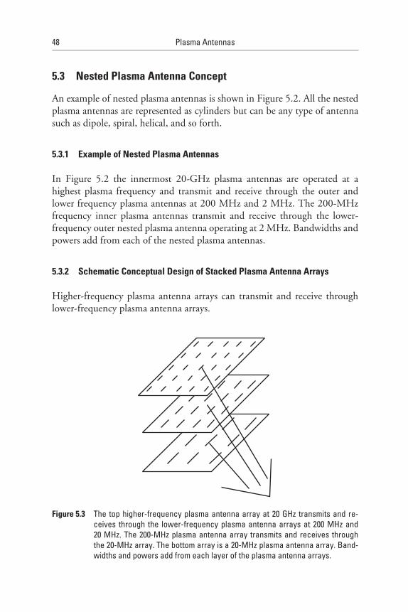
48 PlasmaAntennas
5.3 Nested Plasma Antenna Concept
An example of nested plasma antennas is shown in Figure 5.2. All the nested plasma antennas are represented as cylinders but can be any type of antenna such as dipole, spiral, helical, and so forth.
5.3.1 Example of Nested Plasma Antennas
In Figure 5.2 the innermost 20-GHz plasma antennas are operated at a highest plasma frequency and transmit and receive through the outer and lower frequency plasma antennas at 200 MHz and 2 MHz. The 200-MHz frequency inner plasma antennas transmit and receive through the lower- frequency outer nested plasma antenna operating at 2 MHz. Bandwidths and powers add from each of the nested plasma antennas.
5.3.2 Schematic Conceptual Design of Stacked Plasma Antenna Arrays
Higher-frequency plasma antenna arrays can transmit and receive through lower-frequency plasma antenna arrays.
Figure 5.3 Thetophigher-frequencyplasmaantennaarrayat20GHztransmitsandre-ceives through the lower-frequencyplasmaantennaarraysat200MHzand20MHz.The200-MHzplasmaantennaarraytransmitsandreceivesthroughthe20-MHzarray.Thebottomarrayisa20-MHzplasmaantennaarray.Band-widthsandpowersaddfromeachlayeroftheplasmaantennaarrays.
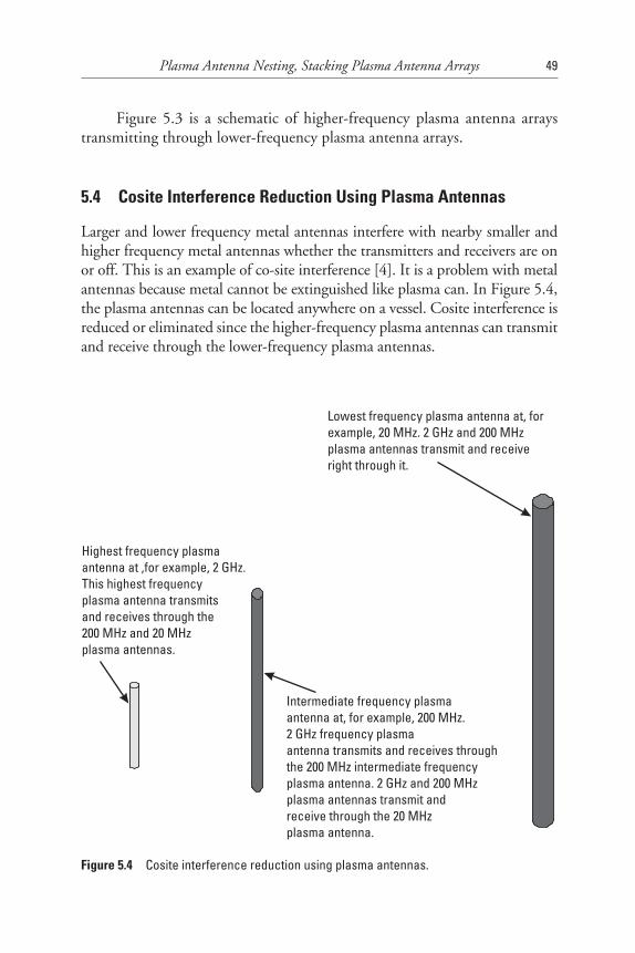
PlasmaAntennaNesting,StackingPlasmaAntennaArrays 49
Figure 5.3 is a schematic of higher-frequency plasma antenna arrays transmitting through lower-frequency plasma antenna arrays.
5.4 Cosite Interference Reduction Using Plasma Antennas
Larger and lower frequency metal antennas interfere with nearby smaller and higher frequency metal antennas whether the transmitters and receivers are on or off. This is an example of co-site interference [4]. It is a problem with metal antennas because metal cannot be extinguished like plasma can. In Figure 5.4, the plasma antennas can be located anywhere on a vessel. Cosite interference is reduced or eliminated since the higher-frequency plasma antennas can transmit and receive through the lower-frequency plasma antennas.
Lowest frequency plasma antenna at, forexample, 20 MHz. 2 GHz and 200 MHzplasma antennas transmit and receiveright through it.
Highest frequency plasmaantenna at ,for example, 2 GHz.This highest frequencyplasma antenna transmitsand receives through the200 MHz and 20 MHzplasma antennas.
Intermediate frequency plasmaantenna at, for example, 200 MHz.2 GHz frequency plasmaantenna transmits and receives throughthe 200 MHz intermediate frequencyplasma antenna. 2 GHz and 200 MHzplasma antennas transmit andreceive through the 20 MHzplasma antenna.
Figure 5.4 Cositeinterferencereductionusingplasmaantennas.

50 PlasmaAntennas
5.5 Plasma Antenna Nesting Experiments
The basic object is to demonstrate that a high-frequency plasma antenna can transmit through an operating low-frequency plasma antenna.
Figure 5.5 is our nested plasma antenna experimental prototype.Two plasma antennas were used at operating transmitting frequencies
of 4 and 8 GHz. The higher frequency plasma antenna was a half-circle of plasma tubes (fluorescent lamps). These tubes are energized by high-current pulses of a 2-ms duration repeated every millisecond, which forms a dense steady-state plasma. The lower-frequency plasma antenna consisted of two tubes directly in front of the broadband receiving microwave horn. Both low and high frequencies are received by a broadband microwave horn, amplified by a traveling wave tube amplifier, and displayed on a panoramic receiver.
The experimental results are shown in Figure 5.6. When the 4-GHz plasma antenna is not energized, the 8-GHz plasma antenna signal appears. However, the 4-GHz signal is not visible, even though the 4-GHz transmit-ter is operating. When the 4-GHz plasma antenna is energized, both the 8- and 4-GHz signals are received. In this case, the 8-GHz plasma antenna signal is penetrating the plasma antenna operating at 4 GHz. Note that the 8-GHz signal is not appreciably attenuated by the operating 4-GHz plasma antenna. The gain for both traces is the same. Only the baseline has been moved to display before and after traces on the same display. The plasma density of the 4 GHz plasma antenna was chosen so that the 8-GHz signal passes through the antenna. This section is related but different to the plasma
Figure 5.5 Ournestedplasmaantennaexperimentalprototype.

PlasmaAntennaNesting,StackingPlasmaAntennaArrays 51
antenna nesting experiment in Section 9.8. Figure 9.18 is similar to Figure 5.6, but different because the lower frequency in Section 9.8 is less than the lower frequency in Section 5.5.
References
[1] Krall, N., and A. Trivelpiece, PrinciplesofPlasmaPhysics, McGraw-Hill Inc., 1973, pp. 151.
[2] Alexeff, I. , and T. Anderson., “Experimental and Theoretical Results with Plasma Antennas,” IEEETransactionsonPlasmaScience, Vol. 34, No. 2, April 2006.
[3] Alexeff, I., and T. Anderson, “Recent Results of Plasma Antennas,” PhysicsofPlasmas, Vol. 15, 2008.
[4] http://www.armymars.net/ArmyMARS/MilInfo/FM11-53-Combat-Net-Radio/app%20b.doc
Figure 5.6 The experimental results of plasma antenna nesting. The top oscilloscopetracesonlyifthe8-GHzplasmaantennaisonandthe4-GHzplasmaantennaisoff.Inthebottomtracebothplasmaantennasareonandthe8-GHzplasmaantennasignal transmits throughthe4-GHzplasmaantennasignalandbotharereceived.Thiscannotbedonewithmetalantennas.


53
6Plasma Antenna Windowing: Foundation of the Smart Plasma Antenna Design
6.1 Introduction
An alternate to the following analysis can be made by using a mutual imped-ance model found in Kraus and Marhefka [1]. This model can be extended from metal antennas to plasma antennas. Using this model, a matrix for cur-rents in the plasma antennas can be used to derive the radiated antenna field. This approach is not given here.
Readers should take note, however, that the impedance is the plasma antenna is reconfigurable, as the derivation in Chapter 3 shows.
Various applications of the smart plasma antenna with the plasma win-dowing concept appear in patents and papers by T. Anderson or T. Anderson et al. [2–14]. An alternative to developing smart plasma antennas is using computer-controlled plasma antenna multipole expansions (see Chapter 10) and computer-controlled smart satellite plasma antennas (see Chapter11).
6.2 The Smart Plasma Antenna Design: The Windowing Concept
Figures 6.1 through 6.4 show the plasma windowing concept. Figures 6.1 and 6.2 are schematics of single lobe, multilobe, and mutiband plasma antennas with the windwoing concept. Figure 6.2 [private communication with Ken Connor, 2004] and Figure 6.3 [private communication with Azimi-Sadjadi

54 PlasmaAntennas
Antenna radiation pattern
Transparent plasmawindow or plasma filter
External plasmablanket or plasma
radome
Internal metal orplasma antenna suchas an omnidirectionalbiconical antenna
Figure 6.1 Schematicofasingle-lobeplasmawindowingantenna.
Figure 6.2 Schematicofamultilobeandamultibandplasmawindowingantenna.

PlasmaAntennaWindowing:FoundationoftheSmartPlasmaAntennaDesign 55
Figure 6.3 Topviewschematicoftheplasmawindowingantenna.
Figure 6.4 Schematicofabeamformingforaplasmawindowingdirectionalantennabyde-activatingtwoplasmatubesthatanantennapatternwithtwolobescanachieve.
Babak, 2005]. The concept of creating antenna array characteristics with or without multiple elements is to surround a plasma antenna by a plasma blan-ket in which the plasma density can be varied. In regions where the plasma frequency is much less than the antenna frequency, the antenna radiation passes through as if a window exists in the plasma blanket. In regions where the plasma frequency is high, the plasma behaves like a perfect reflector with a reactive skin depth. Hence, by opening and closing a sequence of these plasma windows, we electronically steer or direct the antenna beam into any

56 PlasmaAntennas
and all directions. This antenna design has the inherent characteristics of smartness. When the correct DSP with feedback and controls are used, this design converts this plasma antenna design into a smart antenna. The advan-tages of the plasma blanket windowing design are:
1. Beam steering of one omnidirectional antenna in the center with the plasma physics of plasma windowing;
2. A reconfigurable directivity and beamwidth;
3. The ability of the beamwidth to vary from an omnidirectional ra-diation pattern with all the plasma windows open to a directional radiation pattern with less than all the plasma windows open.
The beamwidth is reconfigurable from an omnidirectional radiation pattern with all the plasma windows open (plasma tube or tubes off or at a density or densities below cutoff) or a very directional radiation pattern transmit-ting or receiving through open plasma window (low density plasma) with diminished sidelobes (plasma soft surface effects). This can result in higher directivity and gain than a metal antenna of the same size.
This design can also replace all the metal antenna elements in a con-ventional adaptive array with plasma antenna elements. The advantage of the plasma antenna elements is that any combination of them can be turned on or off (extinquished). Mutual interference among the antenna elements is greatly reduced because the plasma antennas can be created or extinguished on demand. This design can also obtain further resolution and flexibility with even greater degrees of freedoms by replacing the metal antenna elements in a conventional array by the plasma windowing antennas.
6.2.1 Multiband Plasma Antennas Concept
A radiation pattern can transmit and receive through an open plasma FSS window in, for example, in the L, S, and X-bands sequentially in time using software capable of modulating between bands and frequencies. A multiband reception system would eliminate the need to build, transport, and maintain multiple receiving dishes in the field as well as reduce the topside weight and superstructure size on ships.
6.2.2 Multiband and Multilobe or Both Plasma Antennas Concept
Radiation patterns transmitting and receiving through an open plasma filter win-dow is an example in the L, S, and X-bands simultaneously. A multiband recep-
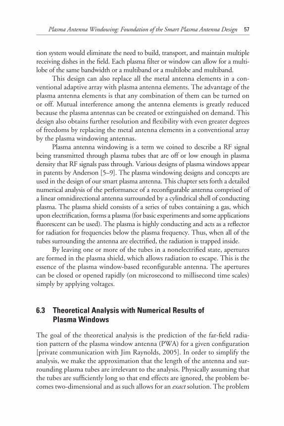
PlasmaAntennaWindowing:FoundationoftheSmartPlasmaAntennaDesign 57
tion system would eliminate the need to build, transport, and maintain multiple receiving dishes in the field. Each plasma filter or window can allow for a multi-lobe of the same bandwidth or a multiband or a multilobe and multiband.
This design can also replace all the metal antenna elements in a con-ventional adaptive array with plasma antenna elements. The advantage of the plasma antenna elements is that any combination of them can be turned on or off. Mutual interference among the antenna elements is greatly reduced because the plasma antennas can be created or extinguished on demand. This design also obtains further resolution and flexibility with even greater degrees of freedoms by replacing the metal antenna elements in a conventional array by the plasma windowing antennas.
Plasma antenna windowing is a term we coined to describe a RF signal being transmitted through plasma tubes that are off or low enough in plasma density that RF signals pass through. Various designs of plasma windows appear in patents by Anderson [5–9]. The plasma windowing designs and concepts are used in the design of our smart plasma antenna. This chapter sets forth a detailed numerical analysis of the performance of a reconfigurable antenna comprised of a linear omnidirectional antenna surrounded by a cylindrical shell of conducting plasma. The plasma shield consists of a series of tubes containing a gas, which upon electrification, forms a plasma (for basic experiments and some applications fluorescent can be used). The plasma is highly conducting and acts as a reflector for radiation for frequencies below the plasma frequency. Thus, when all of the tubes surrounding the antenna are electrified, the radiation is trapped inside.
By leaving one or more of the tubes in a nonelectrified state, apertures are formed in the plasma shield, which allows radiation to escape. This is the essence of the plasma window-based reconfigurable antenna. The apertures can be closed or opened rapidly (on microsecond to millisecond time scales) simply by applying voltages.
6.3 Theoretical Analysis with Numerical Results of Plasma Windows
The goal of the theoretical analysis is the prediction of the far-field radia-tion pattern of the plasma window antenna (PWA) for a given configuration [private communication with Jim Raynolds, 2005]. In order to simplify the analysis, we make the approximation that the length of the antenna and sur-rounding plasma tubes are irrelevant to the analysis. Physically assuming that the tubes are sufficiently long so that end effects are ignored, the problem be-comes two-dimensional and as such allows for an exactsolution. The problem
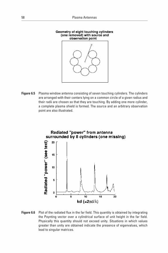
58 PlasmaAntennas
Figure 6.5 Plasmawindowantennaconsistingofseventouchingcylinders.Thecylindersarearrangedwiththeircenterslyingonacommoncircleofagivenradiusandtheirradiiarechosensothattheyaretouching.Byaddingonemorecylinder,acompleteplasmashieldisformed.Thesourceandanarbitraryobservationpointarealsoillustrated.
Figure 6.6 Plotoftheradiatedfluxinthefarfield.Thisquantityisobtainedbyintegratingthe Poynting vector over a cylindrical surface of unit height in the far field.Physically this quantity should not exceed unity. Situations in which valuesgreaterthanunityareobtainedindicatethepresenceofeigenvalues,whichleadtosingularmatrices.

PlasmaAntennaWindowing:FoundationoftheSmartPlasmaAntennaDesign 59
Figure 6.7 Far-fieldradiationpatternsforvarioussolutionsofgeometryillustratedinFigure6.5.
is therefore posed as follows: (1) assume that a wire (the antenna) is located at the origin and carries a sinusoidal current of some specified frequency and amplitude; (2) next assume that the wire (can be a metal or plasma antenna) is surrounded by a collection of cylindrical conductors each of the same ra-dius and distance from the origin; and (3) solve for the field distribution everywhere in space and thus obtain the radiation pattern.
6.3.1 Geometric Construction
One particular configuration for the PWA is illustrated in Figure 6.5 for the case of seven cylinders adopting the following simple geometric construction for creating the plasma shield. Plots of radiated power and radiation patterns of the PWA configuration of Figure 6.5 are given in Figures 6.6 and 6.7. The next geometry of the PWA is given in Figure 6.8 with 15 touching cylinders where one is removed from a 16-cylinder geometry. The radiated power and radiation pattern of the PWA given in Figure 6.9 is given in Figure 6.10. Figure

60 PlasmaAntennas
6.11 shows the half beamwidth versus the wavelength for the PWA configura-tions of Figures 6.5 and 6.8. For a complete shield we assume that N cylinders are placed with their centers lying along a common circle chosen to have the source antenna as its center. Thus, choose some distance from the origin d and divide the circle of radius d into equal segments subtending the angles
2 /l l Nψ π= (6.1)
Figure 6.9 Plotofthefar-fieldfluxradiatedfromthe15-cylinderplasmawindowantenna.AsinFigure6.6,thisplotincludesallsolutionsincludingnonphysicalsolutionsforwhichthefluxexceedsunity.
Figure 6.8 Plasmawindowconsistingof15touchingcylinders.

PlasmaAntennaWindowing:FoundationoftheSmartPlasmaAntennaDesign 61
Figure 6.10 Far-fieldradiationpatternsforthe15-cylinderplasmaantennaforseveralofthesolutionsillustratedinFigure6.9.
where the integer l takes on the values l = 0, 1, …, (N - 1). The apertures are formed by simply excluding various cylinders from consideration.
Until this point, we have considered only touching cylinders; however, there is no need to restrict our attention only to touching cylinders. In the following analysis, it is convenient to specify the cylinder radius through the use of a dimensionless parameter t, which takes on values between zero and unity (i.e., 0 £ t £ 1), where t = 0 corresponds to a cylinder of zero radius (i.e., a wire) and t = 1 corresponds to the case of touching cylinders. More explicitly, the radius of a given cylinder (all cylinder radii assumed to be equal) is given in terms of the parameter t, the distance of the cylinder to the origin d, and the number of cylinders needed for the complete shield N by the expression:
sin( / )a d Nτ π= (6.2)

62 PlasmaAntennas
Defining a number of geometric parameters that are needed in the analysis that follows, the coordinates specifying the center of a given cylinder are given in circular polar coordinates by (d, yl) and in Cartesian coordinates by:
cos(2 / )lxd d l Nπ= (6.3)
and
sin(2 / )lyd d l Nπ= (6.4)
Defining the displacement vector pointing from cylinder l to cylinder q by the equation:
lq q ld d d= −
(6.5)
the magnitude of this vector is given by:
2 1 cos( )lq q ld ψ ψ= − −
(6.6)
Figure 6.11 Beam half-width versus wavelength for the two plasma window antennaconfigurations,definedastheangleatwhichthefar-fieldradiationpatternisreducedbyafactorofone-half.

PlasmaAntennaWindowing:FoundationoftheSmartPlasmaAntennaDesign 63
The angle ylq is subtended by vectors qd
and .qd
In other words, if we
consider the triangle consisting of the three sides ,qd
,ld
and ,lqd
the angle
ylq is the angle opposite to the side .lqd
This angle is easily obtained by the following two relations:
cos( ) cos( ) cos( )lq lq q q l ld d dψ ψ ψ= − (6.7)
and
sin( ) sin( ) sin( )lq lq q q l ld d dψ ψ ψ= − (6.8)
Lastly, defining the coordinates of the observation point relative to the source as well as with respect to coordinate systems centered on the conduct-ing cylinders, the coordinates of the observation point ρ with respect to the source are denoted by (r, f). To specify the observation point with respect to cylinder q, and defining the displacement vector:
q qdρ ρ= − (6.9)
the coordinates of the observation point in the system centered on cylinder q are thus (rq, fq), which are determined in the same way that the coordinates dlq and ylq were obtained earlier.
To complete the specification of the geometric problem and specify the coordinates of the source with respect to each of the coordinate systems centered on the cylinders, obviously, the distance coordinate dls of the source with respect to the coordinate system centered on cylinder l is given by dlq = d. The angular coordinate yls is easily seen to be given by:
ls lψ ψ π= + (6.10)
6.3.2 Electromagnetic Boundary Value Problem
The solution to the boundary value problem is obtained by assuming the cylinders to be perfect conductors, which forces the electric fields to have zero tangential components on the surfaces of the cylinders. Enforcing this con-dition on each of the cylinders leads to N linear equations for the scattering coefficients. The consequence is an N ´ N linear algebraic problem, which is then solved by matrix inversion.
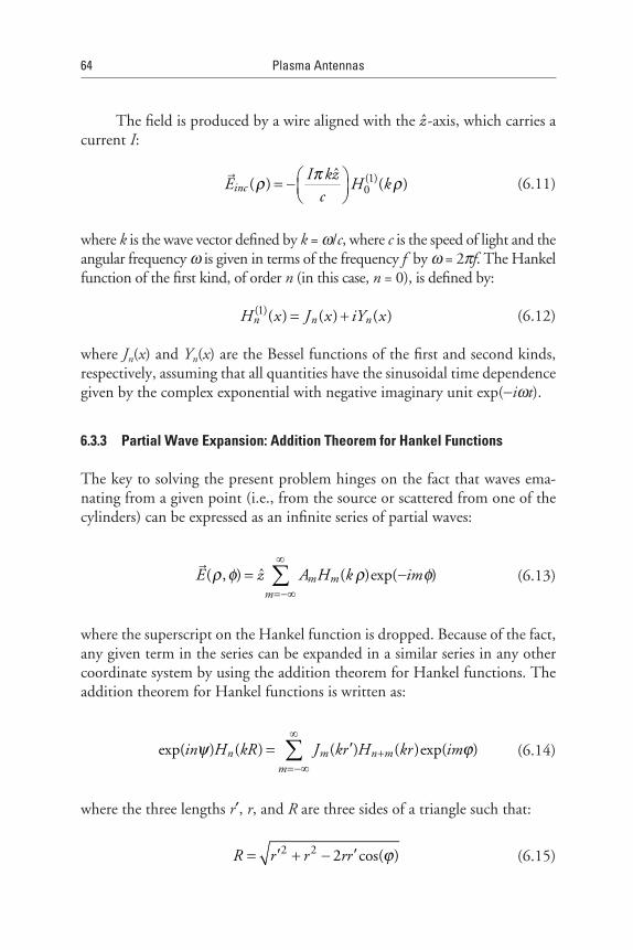
64 PlasmaAntennas
The field is produced by a wire aligned with the z −-axis, which carries a current I:
(1)0
ˆ( ) ( )inc
I kzE H k
cπρ ρ = −
(6.11)
where k is the wave vector defined by k = w/c, where c is the speed of light and the angular frequency w is given in terms of the frequency f by w = 2pf. The Hankel function of the first kind, of order n(in this case, n = 0), is defined by:
(1)( ) ( ) ( )n n nH x J x iY x= + (6.12)
where Jn(x) and Yn(x) are the Bessel functions of the first and second kinds, respectively, assuming that all quantities have the sinusoidal time dependence given by the complex exponential with negative imaginary unit exp(-iwt).
6.3.3 Partial Wave Expansion: Addition Theorem for Hankel Functions
The key to solving the present problem hinges on the fact that waves ema-nating from a given point (i.e., from the source or scattered from one of the cylinders) can be expressed as an infinite series of partial waves:
ˆ( , ) ( )exp( )m mm
E z A H k imρ φ ρ φ∞
=−∞= −∑
(6.13)
where the superscript on the Hankel function is dropped. Because of the fact, any given term in the series can be expanded in a similar series in any other coordinate system by using the addition theorem for Hankel functions. The addition theorem for Hankel functions is written as:
exp( ) ( ) ( ) ( )exp( )n m n m
m
in H kR J kr H kr imψ ϕ∞
+=−∞
′= ∑
(6.14)
where the three lengths r¢, r, and R are three sides of a triangle such that:
2 2 2 cos( )R r r rr ϕ′ ′= + − (6.15)

PlasmaAntennaWindowing:FoundationoftheSmartPlasmaAntennaDesign 65
where r¢ < r and y is the angle opposite to the side r¢. Another way to express this is:
exp( )exp(2 )
exp( )r r i
ir r i
ϕψϕ
′− −=
′− (6.16)
6.3.4 Setting Up the Matrix Problem
A system of N linear equations for the scattering coefficients is obtained by expanding the total field in the coordinate system of each cylinder in turn and imposing the boundary condition that the tangential component of the field must vanish on the surface of each cylinder.
We write the total field as the sum of the incident field incE
plus the scattered field, which is written as:
1
0
( )exp( )N M
qscat n n q q
q n M
E A H k inρ φ−
= =−= ∑ ∑
(6.17)
where the sum has been truncated over the angular variable and retained terms in the range -M £ n £ M.
Next isolate a particular cylinder, say, cylinder l, and express all fields in the coordinate system centered on cylinder l. Upon setting the total field equal to zero and rearranging and obtaining:
−≠ =−
= − − −
+ −
∑ ∑
2
( )exp[ ( ) ] ( )
( )
( )exp( ) ( )
( )
Mm ql
m lq m n lq nmq l n M
mls m ls
m
J kaA i m n H kd A
H ka
I J kaim H kd
H kac
ψ
πω ψ
(6.18)
this can be written compactly in matrix notation as
A D A Kα αβ β α
β= +∑
(6.19)
by adopting the composite index a º (l, m) and b º (q, m). By writing this symbolically as A =DA + K and collecting terms, we obtain (I - D)A = K,
66 PlasmaAntennas
where I is the unit matrix. This equation is solved for the scattering coeffi-cients with matrix inversion to yield:
1( )A I D K−= − (6.20)
6.3.5 Exact Solution for the Scattered Fields
The solution derived in the previous section is formally exact. In practice, one chooses a specific range for the angular sums: -M £ n £ M, which leads to an N(2M + 1)-dimensional matrix problem, the solution of which gives 2M + 1 scattering coefficients .q
nA The quality of the solution is judged by succes-sively increasing the value of M until convergence is reached.
Lastly, it is convenient to use the addition theorem to express all of the scat-tered fields in terms of the coordinate system centered on the source. Thus,
1
0
( )exp( ) ( )exp( )N M M
qn n q q p p
q n M p M
A H k in B H k ipρ φ ρ φ−
= = =−≡∑ ∑ ∑
(6.21)
from which, obtaining the new coefficients as:
1
0
( )exp[ ( ) ]N M
qp n p n q q
q n M
B A J kd i p n ψ−
−= =−
= − −∑ ∑
(6.22)
6.3.6 Far-Field Radiation Pattern
Now for convenience we choose the amplitude of the source current so as to obtain unit flux in the absence of the cylinders. In other words, we choose the source field to be given by:
0
2( )inc
kE H k
cπ ρ= −
(6.23)
Now verifying that this gives unit flux, the far-field limit of the Hankel function is:
2( ) exp[ ( ((2 1) /4]mH k i k m
kρ ρ π
π ρ≈ − +
(6.24)

PlasmaAntennaWindowing:FoundationoftheSmartPlasmaAntennaDesign 67
and the magnetic field is obtained from the electric field as:
inc inc
icB E
ω−= ∇×
(6.25)
The radiation intensity is obtained from these fields by computing the Poynting vector:
[ ]
8c
P E Bπ
∗= ℜ ×
(6.26)
by integrating this over a cylindrical surface of unit height, at a distance r, and obtaining the unit flux as stated.
Now, by extracting a factor of 2 / ,k cπ the total electric field can be expressed as:
0
2( ) ( )exp( )
M
n nn M
kE H k B H k in
cπ ρ ρ φ
=−
= − −
∑
(6.27)
Using this in the earlier expressions gives the Poynting vector. The far-field radiation pattern is obtained by plotting the radial component of the Poynting vector at a given distance (in the far field) as a function of the angle.
6.3.7 Eight-Lobe Radiation Patterns for the Plasma Antenna Windowing Device
Figures 6.12 through 6.19 are plots of multilobe radiation patterns from multiple plasma windows in the plasma windowing antenna.
6.3.8 Dissipation in the Plasma Window Structure: Energy Conservation in an Open Resonant Cavity
Details of research building on previous work with the plasma window structure are now developed. To review, we are considering a structure com-posed of a linear radiating antenna surrounded by plasma tubes. The pur-pose of such a structure is to actively tune the radiation pattern by selectively

68 PlasmaAntennas
“opening” and “closing” apertures in the structure by varying the reflectivity of the plasma tubes comprising the cavity. For example, by de-ionizing the plasma in a single tube (i.e., by turning off the ionizing current source), an aperture is created and a directed beam of radiation is formed. Multilobe radiation patterns are also easily created.
A formalism that can correctly describe the behavior of the structure for all frequencies of excitation is developed. Theorectical results in previous sections of this chapter successfully described the behavior of the structure for frequencies not coincident with cavity resonances. Cavity resonances cor-respond to self-sustaining, localized electromagnetic oscillations that do not radiate. At sufficiently low frequencies there are no cavity resonances. With increasing frequency, however, cavity resonances become more closely spaced and become increasing difficult to avoid. In order to achieve tightly focused
Figure 6.12 Arrangementofplasmatubestoproduceaneight-mainloberadiationpattern.
Figure 6.13 Sixteen-loberadiationpatternforfrequency(kd=14).

PlasmaAntennaWindowing:FoundationoftheSmartPlasmaAntennaDesign 69
radiation patterns, we must work at high frequencies. This situation demands an approach that can correctly describe the behavior of the structure for all frequencies.
For example, consider the radiated power for an eight-cylinder plasma window with one and two apertures (one and two plasma tubes turned off) as illustrated in Figure 6.20.
The solutions (assuming a fixed current strength) are strictly valid only where the radiated power is less than or equal to unity. We see that by open-ing a second aperture (turning off a second plasma tube) there is a larger range for which the solution is not valid. This problem gets progressively worse as the frequency is increased.
Figure 6.14 Furtherfrequencyincrease(kd=15)increasesthemagnitudeofeightofthemainlobeswhiledecreasingthemagnitudeoftheeightothers.
Figure 6.15 Increasingstill(kd=16)makestheeightfoldradiationpatternevenmorepro-nounced.

70 PlasmaAntennas
We now briefly review the previous treatment of the plasma window structure and motivate the present research. In the previous approach we assumed a given current distribution on the radiating antenna. The current on the antenna produced a source field that interacted with the plasma tubes. The starting point for this treatment is the inhomogeneouswave equation for the electric field in the presence of a time-dependent current density. This equation reads:
22
2 24 ( , )
( , )J r t
E r ttc c
ω 𠶶
∇ + =
(6.28)
This equation was solved with a specified form for the right-hand side subject to the boundary condition that the fields vanish on the surface of the
Figure 6.16 Frequencykd=17.
Figure 6.17 Frequencykd=18.

PlasmaAntennaWindowing:FoundationoftheSmartPlasmaAntennaDesign 71
plasma tubes (assumed for simplicity to be perfect conductors). Equation (6.28) however, is not applicable at a cavity resonance. At such a resonance, the right-hand side of this equation vanishes and one must solve the resulting homogeneousequation.
In the present treatment we take a different approach to describe the current on the source antenna. Rather than prescribing a particular current on the source, we instead specify a fixed oscillating driving electric field in the antenna. For such an antenna in free space (i.e., in the absence of the plasma tubes), the driving field sets up the oscillating current and the antenna radiates as usual. Inside the plasma window structure, however, the moving charges comprising the current interact, not only with the driving field but also with the electric fields reflected back from the plasma tubes.
We therefore must set up an equation of motion for the charges in the antenna and include all forces acting on the charges. These forces consist of:
Figure 6.18 Frequencykd=19.
Figure 6.19 Frequencykd=20.
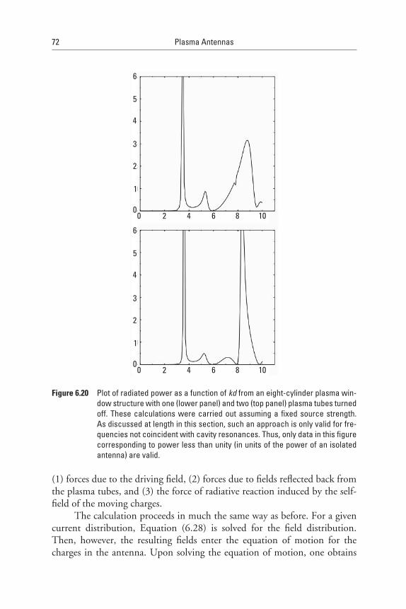
72 PlasmaAntennas
(1) forces due to the driving field, (2) forces due to fields reflected back from the plasma tubes, and (3) the force of radiative reaction induced by the self-field of the moving charges.
The calculation proceeds in much the same way as before. For a given current distribution, Equation (6.28) is solved for the field distribution. Then, however, the resulting fields enter the equation of motion for the charges in the antenna. Upon solving the equation of motion, one obtains
Figure 6.20 Plotofradiatedpowerasafunctionofkdfromaneight-cylinderplasmawin-dowstructurewithone(lowerpanel)andtwo(toppanel)plasmatubesturnedoff.Thesecalculationswerecarriedoutassumingafixedsourcestrength.Asdiscussedatlengthinthissection,suchanapproachisonlyvalidforfre-quenciesnotcoincidentwithcavityresonances.Thus,onlydatainthisfigurecorrespondingtopowerlessthanunity(inunitsofthepowerofanisolatedantenna)arevalid.
Q20: Or do you mean section?

PlasmaAntennaWindowing:FoundationoftheSmartPlasmaAntennaDesign 73
the value of the current, which in turn determines the strength of the fields. As one approaches a cavity resonance, the strength of the reflected field increases and becomes comparable in strength to the driving field. The phase of the reflected field, as well as the self-field (giving rise to radiative reaction), tends to cancel out the influence of the driving field. At a cavity resonance we have two possibilities: (1) either the total current [on the right side of (6.1) goes to zero, or (2) it be-comes out of phase with the driving field. In either case, the driving field does no net work on the current distribution, and in turn there is no radiation despite the presence of the nonzero oscillating fields of the cavity resonance.
We turn now to the technical details of the new approach. First we must consider the phenomenon of radiative reaction induced by the self-field of the oscillating charge. We wish to calculate the work done per unit time by the source field on the charge distribution in the antenna and compare it to the power radiated by the antenna in the far field. We start by considering an isolated linear antenna in free space. If we don’t consider the force of radiative reaction, we are led to the erroneous conclusion that the source field does no work on the charges. We reach this conclusion as follows. If we solve New-ton’s equation of motion for a charge in the presence of the driving field, we find that the resulting current is out of phase with the driving field and thus no net work is done. The radiative reaction force, however, produces a com-ponent of the current that is in phase with the driving field and thus leads to the correct answer for the work done on the charge by the driving field (i.e., the work done per unit time equals the power radiated by the antenna).
In detail, the electric field produced by a linear antenna is given by:
(1)02
ˆ( , ) ( )I
E H zc
πωρ ω ω ρ−=
(6.29)
where I is the current, w is the frequency, c is the speed of light in vacuum, and ρ
is a vector describing the observation point in the plane perpendicular to the axis of the antenna which is taken to be the z-axis. The function on the right-hand side of (6.29) is the Hankel function of the first kind: (1)
0 00 ( ) ( ) ( )H x J x iN x= + , where J0(x) is the zeroth-order Bessel function (not to be confused with the current density) and N0(x) is the Neumann function. The self-field giving rise to radiative
reaction is obtained by evaluating the real part of (1)0 ( )H ω ρ (i.e., 0( )J ω ρ ) on
the antenna axis. The self-field is then:
2self
IE
c
πω−=
(6.30)

74 PlasmaAntennas
If we assume the current to be of the form I(t) = I0sin(wt), the average work done per unit time by the self-field is:
1/ 20
20 2
selfI
dtE Ic
ω πω−⋅ =∫
(6.31)
Since the self-field acts in opposition to the applied field, the amount of work done by the source field is the absolute valueof (6.30), which is exactly equalto the power radiated by the antenna. Thus, energy is conserved.
We now write Newton’s equation of motion for a charge in the antenna in the presence of the source field as well as the self-field:
( )source selfmz q E E= + (6.32)
We first this equation with the source-field only, in order to fix the val-ues of various constants. The desired result is to obtain a current of the form I(t) = I0cos(wt) = Re(I0e–iwt). As we will find, since this current (without the source field) is out of phase with the driving field, we take for simplicity the driving field to be of the form –Re(iE0e–wt) = –sin(wt), and, following stan-dard practice, we work with the complex quantities in solving the equations and take the real parts at the end.
By solving this equation, we find the position versus time z(t); differen-tiating this gives the velocity v(t). We assume a wire of a circular cross-section a. The current density is given by J = qrv where r is the number density of charges in the wire and q is the charge on a given carrier (i.e., electron).
Using these definitions, with the solutions of (6.32) we obtain for the current density
0( ) i tqEJ t e
mωρ
ω−=
(6.33)
The magnitude of the current at the origin is given by multiplying the magnitude of the current density by the cross-sectional area of the wire as:
0 0
qaI E a qz
mρ ρ
ω= =
(6.34)
where in the last equality we have expressed the magnitude of the current in terms of the velocity. Using this value of the current in the definition of the

PlasmaAntennaWindowing:FoundationoftheSmartPlasmaAntennaDesign 75
self-field allows us to express the radiative reaction force as a velocity-depen-dent damping force. The radiative reaction field (with (6.34) substituted into (6.30)) becomes:
2selfqa
E zc
πωρ= −
(6.35)
Using this form gives the equation of motion for a charge in the pres-ence of the driving field and the radiative reaction as:
0i tmz iqE e zω γω−= − − (6.36)
where we have defined the damping constant:
2
a q
c
ρ πγ ≡
(6.37)
Solving (6.36) for the current density, we find the correct result (details not shown) for the work done by the driving field acting on the radiating charges to be given by the absolute value.
Now we generalize to include the influence of the fields reflected back to the source by the plasma tubes. This approach will allow us to correctly describe the situation near a cavity resonance.
From previous reports we found the fields scattered fields from the plasma tubes to be of the form:
1(1)
0
( )exp( )N
qs n n q q
q n
E A H k inρ φ−
== ∑∑
(6.38)
where ,( )q qρ φ are the coordinates of the field point in a system centered on a cylinder (plasma tube) number q and the wave number is defined as k = w/c. The coefficients q
nA are proportional to the net current on the source antenna determined self-consistently including the effects of the scattered fields as well as the radiative reaction field. Thus, we write the coefficients as:
q qn nA zAγω≡ (6.39)

76 PlasmaAntennas
where the coefficient qnA is solved for a fixed current strength by inverting a
matrix problem as described in previous analysis.Now using the addition theorem for Hankel functions, we evaluate the
scattered field of (6.38) at the origin (i.e., on the axis of the source antenna):
(0, ) ( )sE zRω γω ω= (6.40)
where the frequency-dependent function R(w) is given by:
1(1)( ) ( )exp( )
Nqn n q q
q n
R z A H kd inω γω ψ−
= ∑∑
(6.41)
where ( , )q qd ψ
are the coordinates of the cylinder number q in the system centered on the source antenna axis.
Now the complete equation of motion including all fields is written as:
0 (1 ( ))i tmz qE e z Rω γω ω−= − − − (6.42)
This equation is easily solved for the current density:
20( / )
( ) (1 )
i tq E eJ
m g i f
ωρ ωγ γ
−=
+ + − (6.43)
where we have defined the quantities f and g to be the real and imaginary parts of the double summation in (6.41) as:
( )Rf ig
zω
γω≡ +
(6.44)
Note in (6.43) that the real and imaginary parts of the scattered field act in different ways. The real part f is in phase with the radiative reaction force and is of the opposite sign. As we will see, when this quantity cancels the radiative reaction, no net power is radiated and we have localized fields of the cavity resonance. The imaginary part of the reflected field gives rise to

PlasmaAntennaWindowing:FoundationoftheSmartPlasmaAntennaDesign 77
mass renormalization as we see from the term (m + g g) in the denominator of (6.43).
Next we calculate the work done by source field as the time average of the source field times the current density of (6.43). The result is given by:
2 2( / )(1 )
2
I c fP
π ω −=
(6.45)
where the current is given in terms of the current density by multiplying by the cross-sectional area of the wire: I = aJ. Equation (6.45) has the form for an isolated antenna multiplied by the correction factor (1 - f). It is this cor-rection factor that will correctly account for the presence of cavity resonances. Equation (6.45) is the principal result of this section.
Note that from (6.43) and (6.45) two possibilities can occur for cavity resonances. In once case, 1 - f = 0 in (6.45), and no net power is radiated while the current density of is nonzero. This corresponds to a cavity mode with a nonzero field at the presence of the antenna. The other possibility oc-curs when the quantity R(w) diverges. In this case the power vanishes because the denominator of |I|2 diverges faster than the correction factor (1 - f) in (6.45). This corresponds to a cavity resonance with a node at the antenna axis. Lastly, in the absence of the reflecting plasma tubes, f = 0, and we recover the correct result for an isolated radiating antenna.
The problem of a radiating antenna has been formulated in the plasma win-dow structure in order to correctly account for the presence of cavity resonances. This was done by considering the solution of the classical equation of motion for a charge in the antenna in the presence of a driving field in addition to the force of radiative reaction as well as forces due to fields reflected back to the source by the plasma tubes (treated here as perfectly conducting cylinders). The work done by the source field was calculated on the radiating charge and we find it to be of the well-known form for an isolated radiating antenna with a correction due to the cavity fields. It is this correction that will lead to zero radiated fields for frequen-cies corresponding to cavity resonances. It was shown that in the absence of the reflecting cylinders, the correct result for an isolated antenna can be recovered. The new formula was analyzed to show that zero net radiated power can occur for two different kinds of cavity resonances: ones with and without nodes at the position of the radiating antenna. Ongoing research is devoted to proving that the work done by the source field on the radiating charges is correctly equal to the power radiated in the far field.

78 PlasmaAntennas
References
[1] Kraus, J., and R. Marhefka, Antennas for All Applications, 3rd ed., New York: McGraw-Hill, 2001, pp. 444–454.
[2] www.ionizedgasantennas.com.
[3] www.haleakala-research.com.
[4] www.drtedanderson.com.
[5] Anderson, T., “Multiple Tube Plasma Antenna,” U.S. Patent No. 5,963,169, issued Oct. 5, 1999.
[6] Anderson, T., and I. Alexeff, “Reconfigurable Scanner and RFID,” Application Serial Number 11/879,725, Filed 7/18/2007.
[7] Anderson, T., “Configurable Arrays for Steerable Antennas and Wireless Network In-corporating the Steerable Antennas,” U.S. Patent No. 7, 342,549, issued March 11, 2008.
[8] Anderson, T., “Reconfigurable Scanner and RFID System Using the Scanner,” U.S. patent 6,922,173, issued July 26, 2005.
[9] Anderson, T., “Configurable Arrays for Steerable Antennas and Wireless Network In-corporating the Steerable Antennas,” U.S. Patent No. 6,870,517, issued March 22, 2005.
[10] Anderson, T., and I. Alexeff, “Theory and Experiments of Plasma Antenna Radia-tion Emitted Through Plasma Apertures or Windows with Suppressed Back and Side Lobes,” InternationalConferenceonPlasmaScience, 2002.
[11] Anderson, T., “Storage and Release of Electromagnetic Waves by Plasma Antennas and Waveguides,” 33rdAIAAPlasmadynamicsandLasersConference, 2002.
[12] Anderson, T., and I. Alexeff, “Plasma Frequency Selective Surfaces,” InternationalCon-ferenceonPlasmaScience, 2003.
[13] Anderson, T., and I. Alexeff, “Theory of Plasma Windowing Antennas,” IEEEICOPS, Baltimore, June 2004.
[14] http://www.haleakala-research.com/uploads/operatingplasmaantenna.pdf.

79
7Smart Plasma Antennas
7.1 Introduction
This chapter expands on Chapter 6. A smart plasma antenna has been de-veloped [1–5]. Various applications of the smart plasma antenna appear in patents and papers by Anderson or Anderson et al. [3–14].
To get the full appreciation of the smart plasma antenna, please play the video of the smart plasma antenna on www.ionizedgasantennas.com or www.drtedanderson.com.
7.2 Smart Antennas
A smart antenna is a system of antenna arrays with smart signal processing algorithms. The smart antennas are used to identify the direction of arrival of the signal, to calculate beamforming vectors, and to track and locate the antenna beam on the mobile/target. Early smart antennas were designed for governmental use in military applications, which used directed beams to hide transmissions from an enemy. Presently smart antennas may have many ap-plications, including cell phones because they provide greater capacity and performance benefits than standard antennas.

80 PlasmaAntennas
Smart antennas are divided two main types:
1. Switched beam smart antennas in which a decision is made as to which beam to access, at any given point in time, based upon the requirements of the system;
2. Adaptive array smart antennas, which allow the antenna to steer the beam to any direction of interest while simultaneously nulling interfering signals.
7.3 Early Design and Experimental Work for the Smart Plasma Antenna
A prototype smart plasma antenna based on the plasma windowing of Chap-ter 6 has been developed. Figures 7.1 through 7.4 show the initial experimen-tal setups and initial equipment. The object is to have an antenna observe a
Figure 7.1 Photo of the initial construction of the laboratory smart plasma antenna. Ametaldipoleantennaisinthecenterandissurroundedbyfluorescenttubes.
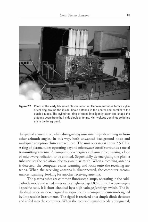
SmartPlasmaAntenna 81
designated transmitter, while disregarding unwanted signals coming in from other azimuth angles. In this way, both unwanted background noise and multipath reception clutter are reduced. The unit operates at about 2.5 GHz. A ring of plasma tubes operating beyond microwave cutoff surrounds a metal transmitting antenna. A computer de-energizes a plasma tube, causing a lobe of microwave radiation to be emitted. Sequentially de-energizing the plasma tubes causes the radiation lobe to scan in azimuth. When a receiving antenna is detected, the computer ceases scanning and locks onto the receiving an-tenna. When the receiving antenna is disconnected, the computer recom-mences scanning, looking for another receiving antenna.
The plasma tubes are common fluorescent lamps, operating in the cold-cathode mode and wired in series to a high-voltage DC supply. To de-energize a specific tube, it is short-circuited by a high-voltage Jennings switch. The in-dividual tubes are de-energized in sequence by a computer, custom-designed by Impeccable Instruments. The signal is received on a simple diode detector and is fed into the computer. When the received signal exceeds a designated,
Figure 7.2 Photooftheearlylabsmartplasmaantenna.Fluorescenttubesformacylin-dricalringaroundtheinsidedipoleantennainthecenterandparalleltotheoutside tubes.Thecylindrical ringof tubes intelligentlysteerandshape theantennabeamfromtheinsidedipoleantenna.High-voltageJenningsswitchesareintheforeground.

82 PlasmaAntennas
adjustable threshold, the computer ceases scanning, and holds this window open. If the received signal subsequently drops below this threshold, the com-puter recommences the scanning process (see Figure 7.4). Beam forming for a plasma windowing directional antenna. The present scanning rate can be adjusted from milliseconds to about a second per tube.
The basic idea is to have an intelligent antenna look in space for a trans-mitter or receiver, lock on to the receiver or transmitter direction when found to increase signal to noise ratio, disconnect from the receiver or transmitter direction when the signal is lost, and resume scanning.
A directional plasma antenna in operating condition, the required scan-ning electronics, and a receiver that detects the desired signal were used. Fig-ure 7.5 is a block diagram of the apparatus desired.
The three items that we have on hand are:
1. The computer input interface: This measures the peak signal from the receiver and inputs this signal into one memory channel in the computer. There will be one memory channel for each angle at which the plasma antenna can be directed. In the present prelimi-
Figure 7.3 Laboratorysetupforearlysmartplasmaantennaexperiments.Anearlysmartplasmaantennaisontheright.High-voltageJenningsswitchesareinthefore-groundofthesmartplasmaantenna.

SmartPlasmaAntenna 83
nary configuration, the signal is a slow pulse of zero to about 50V. A simple diode pulse stretcher to convert the signal to quasi-dc was used.
2. The computer itself: The computer will make one complete scan over all of the included memory channels. It will then compare the signals from all the memory channels. The computer will decide which channel has the largest signal and will lock onto the signal in that channel. It will continue to monitor the input signal. When the input signal falls below a specified threshold (transmitter off ), the lock onto the signal will be terminated, and the computer will resume scanning. The scanning time in this preliminary configura-tion may be quite slow—one channel per second.
3. Thecomputeroutputinterface: Each memory channel should have an output coupler to an element of the plasma antenna. In the pres-ent, temporary configuration, each plasma element is activated by a Jennings high-voltage switch, which requires 110-V AC.
Experimental measurements of the plasma windowing in the smart plasma antenna indicated the directivity as indicated in Figure 7.6.
Figure 7.4 Earlyoperatingunittodrivetheexperimentalsmartplasmaantenna.Thebarlampsshowthesignalstrengthineachchannel.Itislockedonthemiddlechannel.

84 PlasmaAntennas
7.4 Microcontroller for the Smart Plasma Antenna
Today smart antennas have become a serious research and development topic and they are in the process of getting smarter. Smart antennas have the ca-pability to extend the range and increase efficiency of communications for nearly wireless communications technology.
A microcontroller (Figure 7.7) to control the plasma antenna intel-ligently has been built. A BASIC Stamp 2 is used as a microcontroller. A BASIC Stamp includes a BASIC Interpreter chip, internal memory (RAM and EEPROM), a 5-volt regulator, a number of general-purpose I/O pins (TTL-level, 0-5 volt), and a set of built-in commands for math and I/O pin operations. Our BASIC Stamp module is capable of running a few thousand instructions per second and was programmed with a BASIC pro-gramming language. The BASIC Stamp module was connected to a power source and then connected to a PC or laptop and programmed. Then a computer program was written in that particular BASIC Stamp module and was run.
Figure 7.5 Blockschematicofthesmartplasmaantennaproject.

SmartPlasmaAntenna 85
Three input channels (A, B, and C), were used, and more could be added and the system could easily control more channels. The system will detect these input channels, and by comparing signals coming from these channels, our sys-tem will decide to click to a certain switch. The system may repeat this operation in interval times from less than a millisecond to several tens of seconds. The result is that our plasma antenna windowing device acted as smart device.
The plasma windowing device with plasma tubes both parallel and per-pendicular to the antenna polarization has been investigated (see Figure 7.8).
Figure 7.6 Transmittedsignalsfromthesmartplasmaantennathroughaplasmawindowshowingthedirectivity.
Figure 7.7 ABASICStamp2microcontroller.

86 PlasmaAntennas
7.5 Commercial Smart Plasma Antenna Prototype
Figures 7.9 through 7.12 show the smart plasma antenna commercial pro-totype [private communication with Jeff Peck, 2006]. Figure 7.13 shows the ruggedized smart plasma antenna prototype. The smart plasma antenna currently weighs about 15 pounds. It can steer the antenna beam 360° in milliseconds. The future prototypes could steer in microseconds using Fabry-Perot-Etalon effects. It is an intelligent, high-performance steerable antenna with compact size and light weight, and it is stealth and jam-resistant.
7.6 Reconfigurable Bandwidth of the Smart Plasma Antenna
The smart plasma antenna consists of a plasma antenna surrounded by a ring of computer-controlled plasma tubes. If the plasma frequency in this ring
Figure 7.8 Twosuperimposedphotos.Thefirstphotoshowssignalscutoffwiththeelectricfieldperpendiculartotheplasmatubes.Thesecondshowscutoffwiththeelec-tricfieldparalleltotheplasmatubes.Thetimescaleis1millisecondperdivision.Notethatthecutoffislongerforthefieldperpendiculartotheplasmatubes,butthedifferenceisnotsignificant.However,forsmalladvantages,itmaybebetterinsomecircumstancestohavethepolarizationparalleltotheplasmatubesandinothercircumstancesperpendiculartotheplasmatubes.Thiswasat6.5GHz.
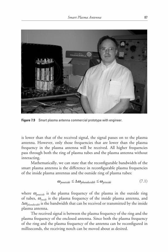
SmartPlasmaAntenna 87
is lower than that of the received signal, the signal passes on to the plasma antenna. However, only those frequencies that are lower than the plasma frequency in the plasma antenna will be received. All higher frequencies pass through both the ring of plasma tubes and the plasma antenna without interacting.
Mathematically, we can state that the reconfigurable bandwidth of the smart plasma antenna is the difference in reconfigurable plasma frequencies of the inside plasma antennas and the outside ring of plasma tubes:
poutside pbandwidth pinsideω ω ω≤ ∆ ≤ (7.1)
where wpoutside is the plasma frequency of the plasma in the outside ring of tubes, winside is the plasma frequency of the inside plasma antenna, and Dwpbandwidth is the bandwidth that can be received or transmitted by the inside plasma antenna.
The received signal is between the plasma frequency of the ring and the plasma frequency of the enclosed antenna. Since both the plasma frequency of the ring and the plasma frequency of the antenna can be reconfigured in milliseconds, the receiving notch can be moved about as desired.
Figure 7.9 Smartplasmaantennacommercialprototypewithengineer.

88 PlasmaAntennas
7.7 Effect of Polarization on Plasma Tubes in the Smart Plasma Antenna
Plasma tubes will intercept microwaves regardless of polarization (Figures 7.14 and 7.15).
A plasma shield has been designed intended to protect sensitive micro-wave equipment from intense electronic warfare signals. A layer of plasma tubes is used as a microwave reflector. The plasma tubes work extremely well
Figure 7.10 Smartplasmaantennacommercialprototype.

SmartPlasmaAntenna 89
in intercepting microwave radiation when the incident wave electric field is parallel to the tubes (see Figure 7.14). However, if the electric field is perpen-dicular to the tubes, the normally induced plasma current cannot flow, and the plasma effects are not expected to appear. When the plasma tubes were experimentally tested with the electric field perpendicular to the tubes, the plasma tubes not only intercepted the microwave signal, but the observed cutoff with a pulsed plasma lasted about twice as long.
Figure 7.11 Smart plasma antenna commercial prototype with open plasma windowindicator.
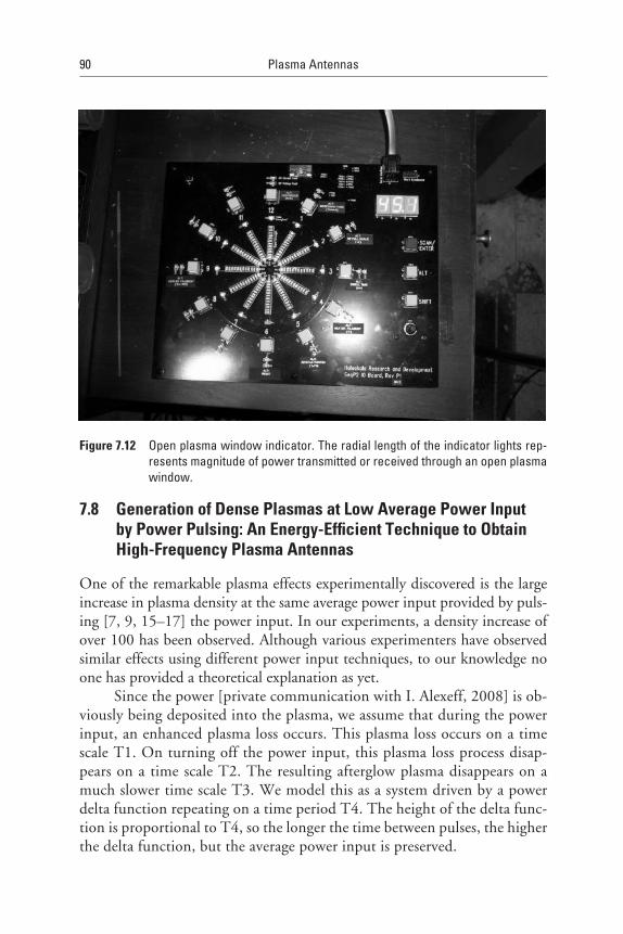
90 PlasmaAntennas
7.8 Generation of Dense Plasmas at Low Average Power Input by Power Pulsing: An Energy-Efficient Technique to Obtain High-Frequency Plasma Antennas
One of the remarkable plasma effects experimentally discovered is the large increase in plasma density at the same average power input provided by puls-ing [7, 9, 15–17] the power input. In our experiments, a density increase of over 100 has been observed. Although various experimenters have observed similar effects using different power input techniques, to our knowledge no one has provided a theoretical explanation as yet.
Since the power [private communication with I. Alexeff, 2008] is ob-viously being deposited into the plasma, we assume that during the power input, an enhanced plasma loss occurs. This plasma loss occurs on a time scale T1. On turning off the power input, this plasma loss process disap-pears on a time scale T2. The resulting afterglow plasma disappears on a much slower time scale T3. We model this as a system driven by a power delta function repeating on a time period T4. The height of the delta func-tion is proportional to T4, so the longer the time between pulses, the higher the delta function, but the average power input is preserved.
Figure 7.12 Openplasmawindowindicator.Theradiallengthoftheindicatorlightsrep-resentsmagnitudeofpowertransmittedorreceivedthroughanopenplasmawindow.

SmartPlasmaAntenna 91
As a first approximation on a single pulse basis, we obtain
2 4
1 5expAG
SS
N T TN T T
= −
(7.2)
where NAG is the afterglow density during pulsing and Nss is the density during steady-state operation. In our experiments, T4 is about 1,000 times T5 (the du-ration of the delta function). If we assume that the fast decay process T1 is of the same approximate length as the time in which this decay process disappears from T2, the calculation in (7.2) yields a density enhancement of about 300. This number agrees with our observed density enhancement. This calculation ignores
Figure 7.13 Ruggedizedsmartplasmaantennaprototype.

92 PlasmaAntennas
Figure 7.14 AttenuationE-fieldparalleltotubes.Asinglepulsewasappliedtotheplasma.Thisexperimentwithanoscilloscopeshows thatwhen theplasmadensitydecreases,cutofftransitionstoareceivedsignalbytheplasma.Theplasmatubesworkextremelywellininterceptingmicrowaveradiationwhentheinci-dentwaveelectricfieldisparalleltothetubes.
Figure 7.15 AttenuationE-fieldperpendiculartotubes.Asinglepulsewasappliedtotheplasma.Theplasmatubesareexperimentallytestedwiththeelectricfieldperpendiculartothetubes.Thisphotoshowsthattheplasmatubesnotonlyinterceptedthemicro-wavesignal,buttheobservedcutoffwithapulsedplasmalastedabouttwiceaslongasthetimethattheplasmadensitydecreasedandthesignalwasreceivedbytheplasma.

SmartPlasmaAntenna 93
plasma left over from the preceding pulse, but most of this is dumped by the ef-fects of the pulse. In any case it can only improve plasma density conditions.
7.9 Fabry-Perot Resonator for Faster Operation of the Smart Plasma Antenna
Fabry-Perot-Etalon effects are well known in optics and Figure 7.16 gives ba-sic instruction of the Fabry-Perot-Etalon effects in the optical region. During transmission of the inside antenna of the smart plasma antenna design, the signal can pass through an open plasma window by turning off the plasma in the plasma window or sufficiently decreasing the density of the plasma in the plasma window to allow the signal to pass through. A faster technique is to increase the plasma density in the plasma tubes so that Fabry-Perot-Etalon effects are met and the signal will pass through. The smart plasma antenna can be programmed to meet the Fabry-Perot-Etalon conditions.
The characteristic decay time of the plasma after power turnoff is typi-cally many milliseconds, so the opening time of such a barrier generally is pre-dicted to also be many milliseconds. However, such a barrier can be opened on a time scale of microseconds. This is done by increasing the plasma den-sity rather than waiting for it to decay. There are two layers of plasma. A standing wave is produced between the two layers that results in microwave transmission, analogous to the transmission found in an optical Fabry-Perot resonator. The secret lies in the boundary layer behavior of the plasma. Once microwave cutoff occurs, one would expect the plasma behavior to be static. What actually occurs is that at microwave cutoff is that the reflection is in phase with the incident wave, in analogy to an open coaxial line. (The elec-tron and displacement currents are equal, but out of phase.) As the plasma density further increases, the reflection smoothly changes from in phase to 180° out of phase, in analogy to a shorted coaxial line. (The reflection current is much greater than the displacement current.)
The boundary condition at a vacuum-plasma interface of the reflected electric field in terms of the incident electric field is:
0
11
ri
E Eiββ
− = + (7.3)
where the phase shift is given by
2
2 1pω
βω
= − (7.4)

94 PlasmaAntennas
The consequence of this phase shift is that, given any kind of a plasma resona-tor, if the plasma density is raised high enough, the resonance required for the Fabry-Perot effect to take place must occur.
The advantage of this method is that the plasma density can be in-creased by ionization in microseconds, releasing the microwave radiation. Normally the release of microwave radiation requires the plasma to decay, which occurs in a time of milliseconds.
Experiments on Fabry-Perot effects have been done in a cylindrical ring of plasma tubes resonance cavity. Radiation escaped in experiments even though those plasma tubes were above microwave cutoff. This behavior may be predicted theoretically in that the phase of the reflection in the cutoff state varies the phase angle from 0° to 180°, causing the resonance in the cavity to form. What this means for plasma application is that microwave emission may be turned on in the ionization time scale of microseconds, rather than in the plasma delay time scale of milliseconds.
The cavity has interior surfaces that reflect a wave, usually electromag-netic, of a specific frequency. When a wave that is resonant with the cavity enters, it bounces back and forth within the cavity with low loss. As more wave energy enters the cavity, it combines with and reinforces the standing wave, increasing its intensity. A common example of cavity resonators in-cludes the klystron tube.
Fabry-Perot cavities are small devices. They are built out of small, half-silvered mirrors. Light entering them gets trapped inside. Once inside a Fabry-Perot cavity, certain wavelengths of light are positively reinforced, while most wavelengths destructively interfere with each other. Fabry-Perot cavities can be used to isolate a single wavelength of light. Because they isolate only one wavelength of light, Fabry-Perot cavities are instrumental in making laser light, wavelength filters, or calibration instruments. Fabry-Perot cavi-ties can be built to pass almost any wavelength of light. Some Fabry-Perot cavities can be controlled by an electronic circuit to block or pass a variable wavelength.
An array of cylindrical plasma tubes may lead to a plasma Fabry-Perot cavity resonator upon excitation of internal electromagnetic waves. When the size of the radius in the cylindrical ring plasma tubes is almost equal by the wavelength of microwave, a resonance behavior has been observed. In such a case the radiation escapes so that even those plasma tubes are above microwave cutoff. This resonance behavior has been observed for some other harmonics. The resonance frequency changes with the diameter of the cylin-drical ring of plasma tubes.

SmartPlasmaAntenna 95
7.9.1 Mathematical Model for a Plasma Fabry-Perot Cavity
Here we try to develop a mathematical model for reflection in the Fabry- Perot cavity resonator. The general equations may be written as:
0 .Eε ρ∇ = (7.5)
E i Bω∇× = (7.6)
0 2
iB J E
c
ωµ∇× = −
(7.7)
. 0B∇ =
By considering 2
1p
pω
εω
= −
, where wp is plasma frequency, and
Figure 7.16 InstructiveschematicfortheFabry-Perot-Etaloneffectinoptics.
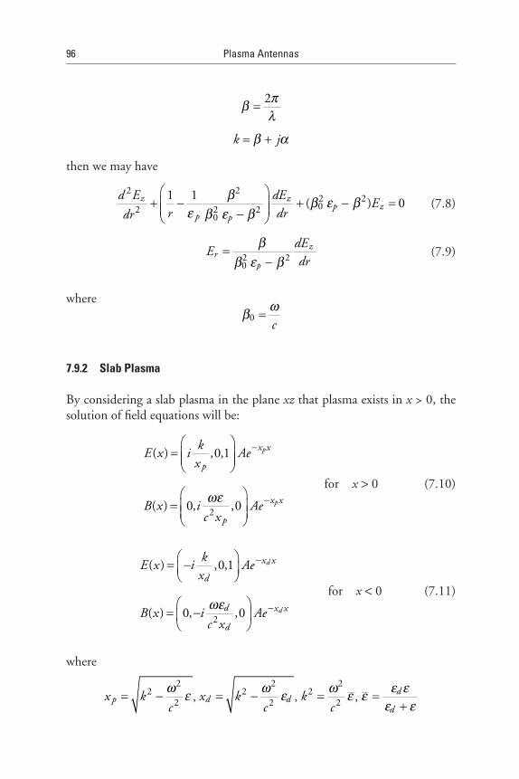
96 PlasmaAntennas
2πβλ
=
k jβ α= +
then we may have
2 22 202 2 2
0
1 1( ) 0z z
p zp p
d E dEE
r drdr
β β ε βε β ε β
+ − + − = −
(7.8)
2 20
zr
p
dEE
drβ
β ε β=
− (7.9)
where
0
cωβ =
7.9.2 Slab Plasma
By considering a slab plasma in the plane xz that plasma exists in x > 0, the solution of field equations will be:
2
( ) ,0,1
( ) 0, ,0
p
p
x x
p
x x
p
kE x i Ae
x
B x i Aec x
ωε
−
−
=
=
for x > 0 (7.10)
2
( ) ,0,1
( ) 0, ,0
d
d
x x
d
d x x
d
kE x i Ae
x
B x i Aec x
ωε
−
−
= −
= −
for x < 0 (7.11)
where
22
2px kc
ω ε= − ,
22
2d dx kc
ω ε= − ,
22
2kc
ω ε= ,
d
d
ε εεε ε
=+

SmartPlasmaAntenna 97
and
1/22
0p
e nm
ωε
=
Then, by considering
e = er + iei
and
2( )( , ) 1
( )p r
ri
ωε ω
ω ω ν= −
+
we will have:
( ) 1/22 2 21
2r i r
cωβ ε ε ε= + + , and ( )1/2
2 2 21
2r i r
cωβ ε ε ε= + −
(7.12)
where
ε ε ε ε εεε ε ε+ +=+ +
2 2
2 2( )
( )r i r d d
rr d i
,
ε εε
ε ε ε=
+ +
2
2 2( )i d
ir d i
Then
εωε ε
=− +( )
pd
xc
,
ω εε ε
=− +( )
dd
dx
c
Then we will have
ω ε ω ε εα εω ε ε ε
− − += − − +
2( )
exp exp2( )
px x r r di
c r d re i x
c 0x > (7.13)
ω ε ω ε εαω ε ε ε ε
− = − + − +
3exp exp
2( ) ( )d d d ix x
c r d r d
e i xc
0x < (7.14)

98 PlasmaAntennas
7.9.3 Cylindrical Plasma
1
1
21
1
20
1
( )( )
( )
( )( )
( )
( )( )
( )
pr R
p
pr r R
p
p pz r R
p
I x rB r B
I x R
I x rkcE r B
I x R
ic x I x rE r B
I x R
ϕ
ωε
ωε
=
=
=
=
=
=
for r< R (7.15)
1
1
21
1
20
1
( )( )
( )
( )( )
( )
( )( )
( )
dr R
d
dr r R
d
p dz r R
d
K x rB r B
K x R
kc K x rE r B
K x R
ic x K x rE r B
K x R
ϕ
ωε
ωε
=
=
=
=
=
=
for r> R (7.16)
Then we will have
β β ε = − 2 2 1/2
0( ) (0) (0) ( )z pE r E I r
ωω
ωω
− −
≈ + −
2
2
2
2
1 1
1 1
pz
p
E (7.17)
In general the governing equations are given below as (7.18) through (7.27).
BE
t∂∇× = −∂
(7.18)
0o o
EB j
tµ µ ε ∂∇× = +
∂
(7.19)
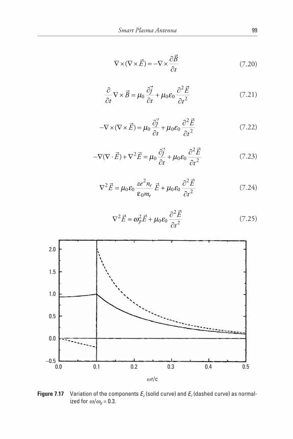
SmartPlasmaAntenna 99
∂∇× ∇× = −∇×∂
( )
BE
t (7.20)
2
0 0 0 2
j EB
t t tµ µ ε∂∂ ∂∇× = +
∂ ∂ ∂
(7.21)
µ µ ε∂ ∂−∇× ∇× = +
∂ ∂
2
0 0 0 2( )j E
Et t
(7.22)
µ µ ε∂ ∂−∇ ∇⋅ +∇ = +
∂ ∂
22
0 0 0 2( )j E
E Et t
(7.23)
2 22
0 0 0 0 20
e
e
ze n EE E
m tµ ε µ ε
e∂∇ = +∂
(7.24)
ω µ ε ∂∇ = +
∂
22 2
0 0 2pE
E Et
(7.25)
Figure 7.17 VariationofthecomponentsEz(solidcurve)andEr(dashedcurve)asnormal-izedforw /wp=0.3.
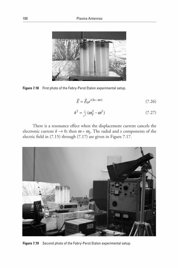
100 PlasmaAntennas
( )
0i kx tE E e ω−=
(7.26)
ω ω= −2
2 2 21 ( )pc
k (7.27)
There is a resonance effect when the displacement current cancels the electronic current k ® 0; then w = wp. The radial and z components of the electric field in (7.15) through (7.17) are given in Figure 7.17.
Figure 7.18 FirstphotooftheFabry-PerotEtalonexperimentalsetup.
Figure 7.19 SecondphotooftheFabry-PerotEtalonexperimentalsetup.

SmartPlasmaAntenna 101
A cylindrical ring of pulsed plasma tubes containing an antenna operat-ing at 3.65 GHz. was tested, as shown in Figure 7.18. The complete installa-tion including the receiving horn is shown in Figure 7.19. A metal reflector behind the plasma tube structure was placed at an angle of 45°, reflecting the backward-directed microwaves upward to prevent interference effects from microwaves reflected from the laboratory wall. Careful tests showed that the antenna radiation primarily was directed upward at an angle of about 30°, so the receiving antenna was oriented accordingly.
The resulting received signal is shown in Figure 7.20. The plasma, when pulsed upon, first completely cuts off the microwave signal. The signal then rises to complete transmission. However, as the plasma further decays, the signal de-creases and then rises again to complete transmission. We interpret the first trans-mission peak to the Fabry-Perot effect. The effect is completely reproducible and varies with the transmitter frequency. The theoretical calculation of the phase shift on the plasma boundary as a function of plasma density is reproduced next.
When working with a complete cylindrical ring of plasma tubes with an antenna in the center, we observe a resonance in that microwaves penetrate the plasma ring when the plasma is above cutoff. Such an effect is observed in
Figure 7.20 Photo of the oscilloscope of Fabry-Perot Etalon experiment. The plasma,whenpulsedupon,firstcompletelycutsoffthemicrowavesignal.Thesig-nalthenrisestocompletetransmission.However,astheplasmafurtherde-cays,thesignaldecreasesandthenrisesagaintocompletetransmission.WeinterpretthefirsttransmissionpeaktotheFabry-Peroteffect.Theef-fectiscompletelyreproducible,andvarieswiththetransmitterfrequency.
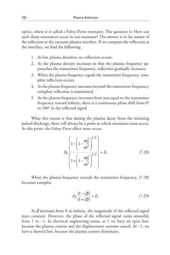
102 PlasmaAntennas
optics, where it is called a Fabry-Perot resonator. The question is: How can such sharp resonances occur in our resonator? The answer is in the nature of the reflection at the vacuum-plasma interface. If we compute the reflection at the interface, we find the following:
1. At low plasma densities, no reflection occurs.
2. As the plasma density increases so that the plasma frequency ap-proaches the transmitter frequency, reflection gradually increases.
3. When the plasma frequency equals the transmitter frequency, com-plete reflection occurs.
4. As the plasma frequency increases beyond the transmitter frequency, complete reflection is maintained.
5. As the plasma frequency increases from just equal to the transmitter frequency toward infinity, there is a continuous phase shift from 0° to 180° in the reflected signal.
What this means is that during the plasma decay from the initiating pulsed discharge, there will always be a point in which resonance must occur. At this point, the Fabry-Perot effect must occur.
ωω
ωω
− − = + −
1/22
2
0 1/22
2
1 1
1 1
p
r
p
E E (7.28)
When the plasma frequency exceeds the transmitter frequency, (7.28) becomes complex.
0
(1 )(1 )
ri
E Eiββ
− =+
(7.29)
As b increases from 0 to infinity, the magnitude of the reflected signal stays constant. However, the phase of the reflected signal varies smoothly from 1 to -1. In electrical engineering terms, at 1 we have an open line, because the plasma current and the displacement currents cancel. At -1, we have a shorted line, because the plasma current dominates.
SmartPlasmaAntenna 103
This shift of phase in the reflected signal introduces many new possi-bilities and applications for our plasma antennas. This means that our switch-ing speeds for the storability of the plasma windowing antenna is greatly enhanced because we do not have to reduce the plasma density to get a trans-mission trough it. Our initial tests show that by using the Fabry-Perot Etalon effect we can increase the plasma antenna switching and steering speeds from milliseconds to microseconds.
More definitive tests on our Fabry-Perot plasma resonator have been made. The idea is that a ring of plasma tubes containing plasma above mi-crowave cutoff may experience a resonance that allows microwave radiation to escape from the resonator have been made. The advantage of this method is that the plasma density can be increased by ionization in microseconds, re-leasing the microwave radiation. Normally the release of microwave radiation requires the plasma to decay, which occurs on a time of milliseconds.
The advanced theory of the microwave plasma Fabry-Perot cavity reso-nator for faster plasma antenna switching speeds has successfully been com-pared to previous experimental results and tests.
7.10 Speculative Applications of the Smart Plasma Antenna in Wireless Technologies
7.10.1 Introduction
This section considers speculative possibilities [private communication with Shivkumar Kalyanaraman, Alejandra Mercado, and Azimi-Sadjadi Babak, 2005] of applications of smart plasma antennas for wireless technologies. The author would like the reader to consider these possibilities while bearing in mind that the smart plasma antenna is untested in these environments.
7.10.2 GPS-Aided and GPS-Free Positioning
Routing methods rely on the position information of nodes of the network. In this section we explain how using smart plasma antennas can enhance the GPS-aided positioning. A method that exploits pattern programmability of smart plasma antennas for GPS-free positioning is proposed.
7.10.2.1 GPS-AidedPositioning
GPS is a widely used positioning technology that allows few meters of ac-curacy when it is used in the stand-alone mode or even millimeter accuracy

104 PlasmaAntennas
when it is used in the differential mode. To reach such accuracy, many sources of position error should be estimated and/or eliminated. These sources of er-ror are differential, receiver clock bias, satellite clock bias, ephemeris error, ionospheric delay, tropospheric delay, integer ambiguity(cycles), and mul-tipath error. Among all these sources of error multipath is the only source that cannot be estimated and eliminated. We remind the reader that posi-tioning technique in GPS algorithm is based on triangulation. It means that a receiver measures its distance from the four or more satellites and based on these measurement finds its location. Any path that is not line of sight does not reflect the true distance between the satellite and GPS receiver. To reduce the effect of multipath error, the GPS antennas are designed so that the mul-tipaths caused by the sea or ground are attenuated, but these antennas cannot eliminated the multipaths caused by other objects such as buildings or hills.
Smart plasma antennas may for the first time provide a practical program-mable antenna pattern that can effectively eliminate all unwanted paths and therefore significantly reduce multipath-induced error. The possibility exists that smart plasma antenna radiation patterns can be programmed so that each satellite in view is assigned a lobe in the pattern. To account for mobile receivers and satellite movement, a beam-steering algorithm could adaptively point these beams towards the associated satellite. Figure 7.21 shows how smart plasma antennas may be used to eliminate multipath in GPS-aided positioning.
7.10.2.2 GPS-FreePositioning
Although the GPS provides acceptable accuracy when four or more satellites are in view, natural or man-made obstacles can easily block the satellite signals,
Figure 7.21 Thesmartplasmaantennamayeliminatemultipath-inducedpositioningerrorinGPSpositioning.

SmartPlasmaAntenna 105
and the GPS signal is not available for positioning inside buildings. Even when a GPS signal is available, it is not always possible to use this technology, because the communication unit may not have enough battery life to power up a GPS receiver or simply because it is not economically feasible to have a GPS receiver in the unit. For all these reasons GPS-free positioning is an important part of academic research and an industrial challenge. A GPS-free positioning tech-nique using a smart plasma antenna may estimate the angle of arrival (AoA) of the received signal and for position estimation.
Since the plasma tube can be activated and deactivated very quickly, the plasma antenna can be considered to be a fast, steerable directional antenna. The access point or a mobile node can obtain information about the location of another node by using the following method. It first sends a message start-ing from the first beam. Then it waits for the node in this direction to respond. Upon receiving the message, a node responds by sending back an acknowledg-ment. The first node then stores the beam direction of that node. After that or a timeout indicating that there is no node residing in this direction, the antenna steers to the next beam and likewise to cover the whole 360°. This steering/response method is used to acquire the spatial signature of each user.
The access point or mobile node sequentially steers the beam towards different directions, so that the entire space is covered. The objective of the localization protocol is to locate all users as fast as possible.
So far, we suppose that acknowledgment in each directional beam is contention-free. We need to consider the situation that there is more than one node in some directions. In this case, some back-off mechanism can be used. The same directional beam of the first node may have to send the message multiple times to locate all the neighbors. The space is successively scanned by a beam until all the direction of neighbors are found and the pro-cedure is repeated for all users equipped with plasma antennas.
Once the network nodes have the AoA information, they can use it in a position estimation. It is assumed that some nodes in the network have their position information beforehand. These nodes are called anchor nodes. Using the anchor nodes, we explain how the other nodes in the network can locate themselves in the same coordinate system.
In Figure 7.22 we assume that nodes 1 and 2 are the anchor nodes. Using a smart plasma antenna, each node can estimate the angel of arrival for i, j = 1, …, 6. It is obvious that node 3 can find its position by just measuring the angle of arrival and knowing the position of nodes 1 and 2. Node 4 can use the position of nodes 3 and 1 and the angle of arrival to estimate its position. This process can be repeated for nodes 5 and 6 and other nodes if applicable. If nodes are capable of measuring their distance from one another, we can use
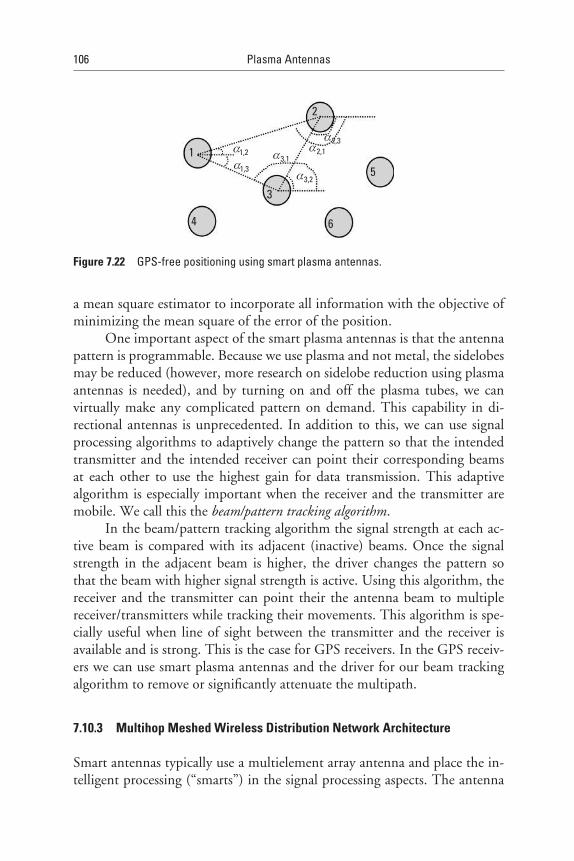
106 PlasmaAntennas
a mean square estimator to incorporate all information with the objective of minimizing the mean square of the error of the position.
One important aspect of the smart plasma antennas is that the antenna pattern is programmable. Because we use plasma and not metal, the sidelobes may be reduced (however, more research on sidelobe reduction using plasma antennas is needed), and by turning on and off the plasma tubes, we can virtually make any complicated pattern on demand. This capability in di-rectional antennas is unprecedented. In addition to this, we can use signal processing algorithms to adaptively change the pattern so that the intended transmitter and the intended receiver can point their corresponding beams at each other to use the highest gain for data transmission. This adaptive algorithm is especially important when the receiver and the transmitter are mobile. We call this the beam/patterntrackingalgorithm.
In the beam/pattern tracking algorithm the signal strength at each ac-tive beam is compared with its adjacent (inactive) beams. Once the signal strength in the adjacent beam is higher, the driver changes the pattern so that the beam with higher signal strength is active. Using this algorithm, the receiver and the transmitter can point their the antenna beam to multiple receiver/transmitters while tracking their movements. This algorithm is spe-cially useful when line of sight between the transmitter and the receiver is available and is strong. This is the case for GPS receivers. In the GPS receiv-ers we can use smart plasma antennas and the driver for our beam tracking algorithm to remove or significantly attenuate the multipath.
7.10.3 Multihop Meshed Wireless Distribution Network Architecture
Smart antennas typically use a multielement array antenna and place the in-telligent processing (“smarts”) in the signal processing aspects. The antenna
Figure 7.22 GPS-freepositioningusingsmartplasmaantennas.
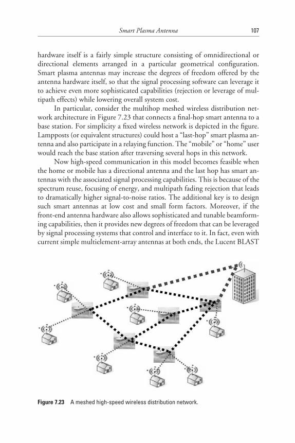
SmartPlasmaAntenna 107
hardware itself is a fairly simple structure consisting of omnidirectional or directional elements arranged in a particular geometrical configuration. Smart plasma antennas may increase the degrees of freedom offered by the antenna hardware itself, so that the signal processing software can leverage it to achieve even more sophisticated capabilities (rejection or leverage of mul-tipath effects) while lowering overall system cost.
In particular, consider the multihop meshed wireless distribution net-work architecture in Figure 7.23 that connects a final-hop smart antenna to a base station. For simplicity a fixed wireless network is depicted in the figure. Lampposts (or equivalent structures) could host a “last-hop” smart plasma an-tenna and also participate in a relaying function. The “mobile” or “home” user would reach the base station after traversing several hops in this network.
Now high-speed communication in this model becomes feasible when the home or mobile has a directional antenna and the last hop has smart an-tennas with the associated signal processing capabilities. This is because of the spectrum reuse, focusing of energy, and multipath fading rejection that leads to dramatically higher signal-to-noise ratios. The additional key is to design such smart antennas at low cost and small form factors. Moreover, if the front-end antenna hardware also allows sophisticated and tunable beamform-ing capabilities, then it provides new degrees of freedom that can be leveraged by signal processing systems that control and interface to it. In fact, even with current simple multielement-array antennas at both ends, the Lucent BLAST
Figure 7.23 Ameshedhigh-speedwirelessdistributionnetwork.

108 PlasmaAntennas
(Bell Labs Layered Space-Time) system has demonstrated tremendous spec-tral efficiency of 20 bits/Hz.
In wireless communications that employ smart antennas, the bases use signal processing techniques to virtually direct the antenna array gain lobes towards the direction of the desired signals, as well as directing the gain nulls towards the direction of interfering signals. Since wireless signals experience multipath scattering, the most prominent multipath signals can be used by a RAKE receiver to enhance the signal to interference and noise ratio (SINR) and thus improve the quality of the link. In such a setting, the base would use a training sequence to determine the direction of the desired multipath signals and direct the lobes of the antenna array towards them.
The number of lobes that can be directed and the number of nulls de-pends on the number of antenna elements in the array. The beamwidth of each lobe depends on the distance between the elements. A higher number of an-tenna elements provide a higher number of lobes to capture several multipath and thus improve the SINR (signal to interference and noise ratio). However, the increase in antenna elements also implies a higher computational cost, since the dimension of the problem increases with the number of antennas.
7.10.4 Reconfigurable Beamwidth and Lobe Number
The beamwidth of the antenna array lobes is chosen so as to minimize the gain towards interfering signals. The narrower the beamwidth, the more iso-lation is provided for the desired signal. However, we have another trade-off, since a narrow beamwidth requires longer training signals to secure the direction of the desired signal. An unreliable estimate of the desired signal direction with a narrow beam may result in severe attenuation of the desired signal, which defeats the purpose of the antenna array.
A smart plasma antenna allow new degrees of freedom and simulate the gains (such as distance, bandwidth, and efficiency) achievable using outdoor fad-ing and propagation models and advanced signal processing capabilities [e.g., multiple-input-multiple-output (MIMO) processing]. The challenge is to choose an array configuration that provides adequate SINR levels while requiring a low computational cost. The utility of this arrangement can be seen in Figure 7.24.
Most communications systems experience peak time periods as well as low demand periods. During the peak hours, the system resources are strained to provide adequate SINR levels. Even with code division multiple access (CDMA) systems, the cross-correlation between user codes is not zero, so the presence of a large number of undesired signals increases the interference. In

SmartPlasmaAntenna 109
this case, we would want very narrow gain lobes to attenuate as many undesired signals as possible. This can be appreciated in Figure 7.24(a). Also in Figure 7.24(a), we see that the presence of a large number of scattering surfaces can be used with BLAST to increase the signal strength. Both of these techniques will improve the link quality, but they will require a large number of calculations.
Figure 7.24(b) shows the opposite situation with few interferers and fewer scattering surfaces. In this situation, we may significantly reduce the complexity of an antenna array problem by using fewer and wider lobes.
The signal-to-noise ratio levels and directions of service can be deter-mined by performing a 360° sweep by each of our smart antennas. In order to distinguish between users of a given sector, as well as lower power usage, a user spreading code can be applied to users of each sector.
This setup provides mobility, since the periodic scanning performed by our smart antennas allows all users as well as all ad hoc nodes to move about without losing the network contact. Each user may be served by any node, which allows for additional flexibility.
Figure 7.24 (a)Antennalobesforpeakhourservicewithmanyinterferingsignalsormanyreflectingsurfaces.(b)Antennalobesforalowdemandperiodorfewreflect-ingsurfaces.

110 PlasmaAntennas
7.10.5 Adaptive Directionality
The adaptive directionality of the smart plasma antennas provides a plethora of advantages. The directivity of each antenna beam minimizes the power levels broadcast that might interfere with adjacent users. In this sense, it pro-vides a form of SDMA. The directivity of the antenna also reduces the power levels that could be detected by unfriendly agents. The adaptive nature of the smart plasma antenna allows the beam to follow the user with a minimum of computation required, as well as to alter the beamwidth depending on if the user is in an area of high user density or requiring greater stealth, where the beam can be made very narrow, or if the user is relatively isolated moving at a great speed, where the beam can be made wider.
In order to further reduce the transmission power levels, thus conserv-ing battery power and concealing the position of the users and nodes, a low spreading gain code can be applied to each user’s signal. The low gain permits us to maintain a high data rate. The highly directional property of our smart antenna does not require a high gain for multiple access. A low tap Walsh code would be enough to permit very low transmission levels, and good pro-tection for each user. In addition, automatic power control can be imple-mented to decrease the collective power transmission of the entire network.
In a military setting, where our goals are to provide as much flexibility, mobility, stealth, and protection from jamming as possible, we tailor our design to meet these needs. We consider a wireless ad hoc network, where there are several nodes deployed that provide a network backbone. An example is the Humvees in Figure 7.25. Each Humvee is equipped with a smart plasma an-
Figure 7.25 Smartplasmaantennawithavariablenumberoflobeswithadaptivebeam-widthsanddirections.

SmartPlasmaAntenna 111
tenna, where each of our smart plasma antennas can create a variable number of antenna gain lobes of adaptive beamwidth and direction. Each soldier has a low power omnidirectional antenna that is served by the Humvee that can offer the best signal-to-noise ratio and has the capacity to serve that user.
The signal-to-noise ratio levels and directions of service can be deter-mined by performing a 360° sweep by each of our smart antennas. In order to distinguish between users of a given sector, as well as lower power usage, a user spreading code can be applied to users of each sector.
This setup provides mobility, since the periodic scanning performed by smart antennas allows all users as well as all ad hoc nodes to move about without losing the network contact. Each user may be served by any node, which allows for additional flexibility.
7.10.6 Cell Tower Setting
In a civilian setting, where goals are to provide low cost and flexibility, we can use the directivity of a smart antenna as a form of implementing SDMA. Figure 7.26 shows an example of this.
In this case, consider the angle of service for each user can be estimated by a pair of omnidirectional antennas placed on the same tower. This setup allows the array of smart antennas to provide uninterrupted service to users without having to estimate the direction of service. The adaptive beamwidth can be ad-justed to accommodate users who are in close proximity, providing protection from interference for each user. The variable number of beams from our smart antenna allows the base to service a variable number of users at diverse locations.
Figure 7.26 Smartplasmaantennasoncelltowers.
112 PlasmaAntennas
This eliminates the need for a technician to install additional antennas or make changes when new users initiate service or when other users terminate service.
References
[1] http://ieeexplore.ieee.org/Xplore/login.jsp?url=http%3A%2F%2Fieeexplore.ieee.org%2Fiel5%2F4345408%2F4345409%2F04345600.pdf%3Farnumber%3D4345600&authDecision=-203.
[2] http://www.haleakala-research.com/uploads/operatingplasmaantenna.pdf.
[3] www.ionizedgasantennas.com.
[4] www.haleakala-research.com.
[5] www.drtedanderson.com.
[6] Anderson, T., “Multiple Tube Plasma Antenna,” U.S. Patent No. 5,963,169, issued Oct. 5, 1999.
[7] Anderson, T., and I. Alexeff, “Reconfigurable Scanner and RFID,” Application Serial Number 11/879,725, Filed 7/18/2007.
[8] Anderson, T., “Configurable Arrays for Steerable Antennas and Wireless Network Incorporating the Steerable Antennas,” U.S. Patent No. 7, 342,549, issued March 11, 2008.
[9] Anderson, T., “Reconfigurable Scanner and RFID System Using the Scanner,” U.S. patent 6,922,173, issued July 26, 2005.
[10] Anderson, T., “Configurable Arrays for Steerable Antennas and Wireless Network Incorporating the Steerable Antennas,” U.S. Patent 6,870,517, issued March 22, 2005.
[11] Anderson, T., and I. Alexeff, “Theory and Experiments of Plasma Antenna Radia-tion Emitted Through Plasma Apertures or Windows with Suppressed Back and Side Lobes,” InternationalConferenceonPlasmaScience, 2002.
[12] Anderson., T., “Storage and Release of Electromagnetic Waves by Plasma Antennas and Waveguides,” 33rdAIAAPlasmadynamicsandLasersConference, 2002.
[13] Anderson, T., and I. Alexeff, “Plasma Frequency Selective Surfaces,” InternationalCon-ferenceonPlasmaScience, 2003.
[14] Anderson, T., and I. Alexeff, “Theory of Plasma Windowing Antennas,” IEEEICOPS, Baltimore, MD, June 2004.
[15] I. Alexeff, “Pulsed Plasma Element,” US patent 7,274,333, issued September 25, 2007.
[16] T. Anderson, “Tunable Plasma Frequency Devices,” US patent, 7,292,191, issued November 6, 2007.
[17] T. Anderson, “Tunable Plasma Frequency Devices,” US patent, 7,453,403, issued November 18, 2008.
113
8Plasma Frequency Selective Surfaces
8.1 Introduction
Plasma frequency selective surfaces [1] use plasma as a substitute for metal in a frequency selective surface (FSS). Frequency selective surfaces have been used for filtering electromagnetic waves. Each FSS layer has to be modeled using numerical methods and the layers are stacked in such a way to cre-ate the desired filtering. Genetic algorithms are used to determine the stack-ing needed for the desired filtering. This is a complicated and numerically expensive process. A method is developed to replace metal in an FSS with plasma elements. The plasma frequency selective surfaces can be tuned to a desired filtering by varying the density in the plasma elements. This could save much of the routine analysis involved in the standard analysis of conven-tional FSS structures. The user simply tunes the plasma to get the filtering desired. Plasma elements offer the possibility of improved shielding along with reconfigurability and stealth. Plasma FSS can be made transparent by turning the plasma off. This extends our previous scientific achievements in the development of the plasma antenna.
As the density of the plasma is increased, the plasma skin depth becomes smaller and smaller until the elements behave as metallic elements and we create filtering similar to FSS with metallic elements. Up until the metallic mode for the plasma, our theory and experiments showed that the plasma FSS had a continuous change in filtering. A basic mathematical model for a plasma FSS is developed by modeling the plasma elements as half-wavelength
114 PlasmaAntennas
and full-wavelength dipole elements in a periodic array on a dielectric sub-strate. The theoretical model with numerical predictions predicted results in good agreement with our experiments on the plasma FSS. Theoretically Floquet’s theorem is used to connect the elements. The transmission and re-flection characteristics of the plasma FSS as a function of plasma density are developed. Frequencies from around 900 MHz to 12 GHz are utilized with a plasma density around 2 GHz. The plasma tubes continuously vary the plasma density and observe the tunability of the reflection and transmission of electromagnetic waves. As the plasma density decays, the amount of trans-mitted electromagnetic energy increases as expected. However, at electromag-netic signals at frequencies well above the plasma frequency, the plasma FSS is transparent. The polarization of the transmitting antenna is rotated by 90° and produces a similar but reduced effect.
An array of plasma frequency selective surfaces was modeled. Similarly, A plasma FSS has been made in the laboratory. The theory and experiment were in close agreement. The plasma FSS is unique and new to the field of electromagnetic filtering. The potential payoff for this technology is high and the risk is moderate. It is moderate since we have developed plasma antennas with transmitters, but the plasma FSS is in some ways easier to develop since it does not require transmitters.
The plasma FSS can shield antennas, military electronics, and radar sys-tems in a tunable way. If no shielding is needed, turning the plasmas off causes the shield to be invisible. Plasma FSS allows users to filter out any undesirable radiation, but at the same time allows users to enable operations outside that band. The potential for technology transfer is significant since the plasma FSS can be tuned to filter out unwanted radiation from commercial products or tuned to filter electromagnetic emissions to meet FCC EMC requirements.
8.2 Theoretical Calculations and Numerical Results
Central to the theoretical modeling is the numerical calculation of the scaling function shown in Figure 8.1. An FSS dipole array consists of a periodic ar-ray of vertically aligned scattering elements. In traditional FSS structures, the scattering elements would be made of some material possessing good electri-cal conductivity (and thus high reflectivity).
For a plasma FSS structure, we imagine a scattering element to consist of gaseous plasma contained in a tube. The purpose of the present investiga-tion is to determine the electromagnetic scattering properties of the array as a function of the reflectivity of the plasma elements.

PlasmaFrequencySelectiveSurfaces 115
8.2.1 Method of Calculation
The response (reflection and transmission) of the plasma FSS is calculated in two stages: (1) the response for a perfectly conducting structure is given, and then (2) we scale the reflectivity by a function that depends on the incident frequency and the plasma frequency so as to account for the scattering prop-erties of the plasma. Details of these two steps will now be presented [private communication with Jim Raynolds].
8.2.1.1 PeriodicMomentMethod
In the first stage of calculation, we use the Periodic Moment Method as de-scribed in [2]. The elements are approximated as thin flat wires. The scat-tered electric field produced by an incident plane wave of a single frequency is given by:
ˆ
|| ||ˆ ˆ( ) [( )( ) ( )( )]2
j R r
Ax y yk n
Z eE R I n P n P
D D r
β ±− ⋅∞ ∞
⊥ ± ⊥ ±=−∞ =−∞
= − +∑ ∑ (8.1)
The quantities in this equation are defined as follows. The quantity IA is the current induced in a single element by the incident plane wave (see [2]), Z is the impedance of the medium that we take to be free space (Z = 377W), R is the position vector of the observation point, and the scattering vector is defined by:
± = ± +ˆ ˆ ˆ ˆx y zr xr yr zr (8.2)
with
= +x x
xr s k
Dλ
,
= +z zz
r s nDλ
(8.3)
and
2 2
1y x zx z
r s k s nD Dλ λ = − + − +
(8.4)
In these equations, sx and sz are the components of the unit vector speci-fying the direction of the incident plane wave. The array is assumed to lie in the x-z plane with repeat distances Dx and Dz, and the directions ± y indicate the forward and backscattering directions, respectively. Note that for suf-ficiently high values of the integers, n and k, the scattering vector component ry becomes imaginary corresponding to evanescent modes.
116 PlasmaAntennas
The remaining quantities (in the square brackets of the expression for the scattered field) are related to the way in which the incident electric field generates a voltage in an array element as described in detail in [2]. The volt-age induced in a scattering element by the incident field is given by:
ˆ( ) ( )V R E R pP= ⋅ (8.5)
where ( )E R is the electric field vector of the incident plane wave, p is a unit vector describing the orientation of the scattering element, and P is the pat-tern function for the scattering element and is defined by:
ˆ ˆ1( )
( )j lp st
tElement
P I l e dlI R
b− ⋅= ∫ (8.6)
where It(l) is the current distribution on the element located at ,R ( )tI R is the current at the terminals of the scattering element (e.g., at the center of a dipole antenna), s is the unit vector denoting the plane wave incident direc-tion, and b = 2p/l is the wave number. The unit vectors ⊥ n and ||n, which describe the electric field polarization, are defined by:
2 2
ˆ ˆˆ z x
x z
xr zrn
r r⊥
− +=+
(8.7)
and
⊥ = × = − + + − +
2 2||
2 2
1ˆ ˆ ˆ ˆ ˆ ˆ( ) .x y x z y zx z
n n r xr r y r r zr rr r
(8.8)
The quantities ^P and ||P are given by multiplying the pattern function by the appropriate direction cosine: ˆ ˆ ,P p nP⊥ ⊥= ⋅ and || ||ˆ ˆP p nP= ⋅ The ef-fective terminal current IA, which enters the equation for the scattered electric field, is obtained from the induced voltage and the impedance as:
=
+A
A L
VI
Z Z (8.9)
where ZL is the self-impedance of the scattering element andZA is the imped-ance of the array.
As in all moment methods, some approximation must be made regard-ing the detailed current distribution on the scattering elements. In order to

PlasmaFrequencySelectiveSurfaces 117
calculate the pattern function, we assume the current distribution to be a superposition of current modes. The lowest-order mode is taken to be a sinu-soidal distribution of the form:
=0( ) cos( / )I z z lπ (8.10)
where we assume the scattering element to be a conductor of length l centered at the origin. Thus, the lowest-order mode corresponds to an oscillating cur-rent distribution of wavelength l = 2l. This lowest-order mode gives rise to a radiation pattern equivalent to a dipole antenna with a current source at the center of the dipole. In effect, this mode divides the scattering elements of Figure 8.2 into two segments. The next two higher-order modes are con-structed by dividing each half of the scattering element into two more seg-ments. These modes are written as:
= ∓1,2( ) cos[2 ( /4)/ ]I z z l lπ (8.11)
Physically these modes correspond to current distributions of wave-length l = l centered at ± l/4. The solution of the problem is then obtained by solving a matrix problem to determine the coefficients of the various modes in the expansion of the currents. For the frequencies considered in this chapter, only the lowest-order mode is considered making the calcula-tions extremely fast.
8.2.2 Scattering from a Partially Conducting Cylinder
In order to calculate the reflection from an array of plasma elements, we make the physically reasonable assumption that (to a first order) the induced current distribution in a partially conducting plasma differs from that of a perfectly conducting scattering element only to the extent that the amplitude is different. In the limit of high conductivity, the current distribution is the same as for a perfect conductor, and in the limit of zero conductivity, the current amplitude is zero.
The scattered electric field is directly proportional to the induced cur-rent on the scattering element. In turn, the reflectivity is thus directly propor-tional to the square of the induced current in the scattering element. Thus, to find the reflectivity of the plasma array, we determine the functional depen-dence of the induced squared current versus the electromagnetic properties of the plasma and scale the reflectivity obtained for the perfectly conducting case accordingly.

118 PlasmaAntennas
In order to obtain the scaling function for the squared current, we consider the following model problem. The problem of scattering is solved from an infinitely extended dielectric cylinder possessing the same dielectric properties as a partially ionized, collisionless plasma. Assuming the dielectric function for the plasma takes the following form:
= −
2
2( ) 1 pνε ω
ν (8.12)
where n is the frequency of the incident electromagnetic wave and np is the plasma frequency defined by:
=
21 42
pne
mπν
π (8.13)
where n is the density of ionized electrons, and e and m are the electron charge and mass, respectively. A good conductor is characterized by the limit of large plasma frequency in comparison to the incident frequency. In the limit in which the plasma frequency vanishes, the plasma elements become completely transparent.
Turning to the solution of the problem of scattering from a partially conducting cylinder, the conductivity and thus the scattering properties of the cylinder are specified by the single parameter np. Solving the wave equa-tion for the electric field:
∂∇ =∂
22
2 21 D
Ec t
(8.14)
subject to the boundary conditions that the tangential electric and magnetic fields must be continuous at the cylinder boundary, considering the scatter-ing resulting from the interaction of the cylinder with an incident plane wave of a single frequency. Therefore, assuming all fields to have the harmonic time dependence:
−i te ω (8.15)
where w = 2pn is the angular frequency, we are adopting the physics conven-tion for the time dependence. Personnel more familiar with the electrical engineering convention can easily convert all subsequent equations to that convention by making the substitution i ® - j.
PlasmaFrequencySelectiveSurfaces 119
Next we assume the standard approximation relating the displacement field to the electric field via the dielectric function:
=( ) ( ) ( )D Eω ε ω ω (8.16)
By imposing cylindrical symmetry, the wave equation takes the form of Bessel’s equation:
∂ ∂ ∂+ + + =∂∂ ∂
2 22
2 2 21 1
0E E E
k Eερ ρρ ρ ϕ
(8.17)
where k = w/c and ( r, j) are cylindrical polar coordinates. The general so-lution of this equation consists of linear combinations of products of Bes-sel functions with complex exponentials. The total field outside the cylinder consists of the incident plane wave plus a scattered field of the form:
∞
=−∞= + ∑cos ( )ik im
out m mm
E e A H k eρ ϕ ϕρ (8.18)
where Am is a coefficient to be determined and Hm(kr) = Jm(kr) + iYm(kr) is the Hankel function that corresponds to outgoing cylindrical scattered waves. The field inside the cylinder contains only Bessel functions of the first kind since it is required to be finite at the origin:
∞
=−∞= ∑ ( ) im
in m mm
E B J k e ϕρ ε (8.19)
To facilitate the determination of the expansion coefficients Am and Bm, the incident plane wave is given as an expansion in the Bessel functions:
∞
=−∞= ∑cos ( )ik m
mm
e i J kρ ϕ ρ (8.20)
To enforce continuity of the electric field at the boundary of the cylinder:
= = =( , ) ( , )in outE a E aρ ϕ ρ ϕ (8.21)
where the cylinder is assumed to have radius a. The next boundary condi-tion is obtained by imposing continuity of the magnetic field. From one of Maxwell’s equations (Faraday’s law), we obtain:

120 PlasmaAntennas
= − ∇×(1/ )H i k E (8.22)
The electric field is assumed aligned with the cylinder axis (TM polar-ization). This is the only case of interest since the scattering of the TE wave is minimal. The tangential component of the magnetic field is thus:
∂= − − ∂ (1/ ) zE
H i kϕ ρ (8.23)
By imposing the continuity of this field along with the continuity of the electric field, the following set of equations that determine the expansion coefficients is obtained:
+ =( ) ( ) ( )mm m m mi J ka A H ka B ka ε (8.24)
and
′ ′ ′+ =( ) ( ) ( )mm m m m mi J ka A H ka B J ka ε ε (8.25)
where the primes on the Bessel and Hankel functions imply differentiation with respect to the argument.
These equations are easily solved for the expansion coefficients:
( ( ) ( ) ( ) ( ))
( ( ) ( ) ( ) ( ))
mm m m m
mm m m m
i J ka J ka J ka J kaA
H ka J ka H ka J ka
ε ε εε ε ε
′ ′− −=′ ′−
(8.26)
and
′ ′−=′ ′−
( ( ) ( ) ( ) ( ))
( ) ( ) ( ) ( )
mm m m m
mm m m m
i J ka H ka J ka H kaB
H ka J ka H ka J kaε ε ε (8.27)
Inspection of these coefficients shows that in the limit e ® 1 (i.e., zero plasma frequency) we obtain Am ® 0 and Bm ® im. Thus, in this limit, the scattered field vanishes and the field inside the cylinder simply becomes the incident field as expected.
The opposite limit of a perfectly conducting cylinder is also established fairly easily but requires somewhat more care. Consider first the field inside the cylinder, which must vanish in the perfectly conducting limit. A typical term in the expansion of the electric field inside the cylinder is of the form:

PlasmaFrequencySelectiveSurfaces 121
( )m mB J kρ ε (8.28)
The perfect conductivity limit corresponds to taking the limit np ® ¥ at fixed n. In this limit →− 2 2/ ,pε ν ν and thus → / .piε ν ν For a large imaginary argument, the Bessel functions diverge exponentially. Therefore:
→ →
( ) 0m m
pB J k O
nρ εn
(8.29)
Lastly, we must establish that the tangential electric field just outside the cylinder vanishes in the perfect conductivity limit as expected. Using the fact that the Bessel functions diverge exponentially for large imagi-nary argument gives the following limit for the scattered wave expansion coefficient:
−→ ( )( )
mm
mm
i J kaA
H ka (8.30)
Thus, a typical term in the expansion for the scattered wave, evaluated just outside the cylinder, has the following limit:
→−( ) ( )mm m mA H ka i J ka (8.31)
which exactly cancels the corresponding term in the expansion of the incident plane wave.
The scaling function defined next is used for the analysis of the scatter-ing from a partially conducting cylinder to obtain a reasonable approxima-tion to the scattering from a partially conducting plasma FSS array based on the computed results for a perfectly conducting array.
Proceed based on the following observations/assumptions:
1. The reflectivity of the plasma FSS array is determined entirely in terms of the scattered field in contrast to the transmitted field, which depends on both the incident and scattered fields.
2. The shape of the current modes on the partially conducting (plasma) FSS array is the same as for the perfectly conducting array.
3. The only difference between the partially conducting and perfectly conducting arrays is the amplitude of the current modes.
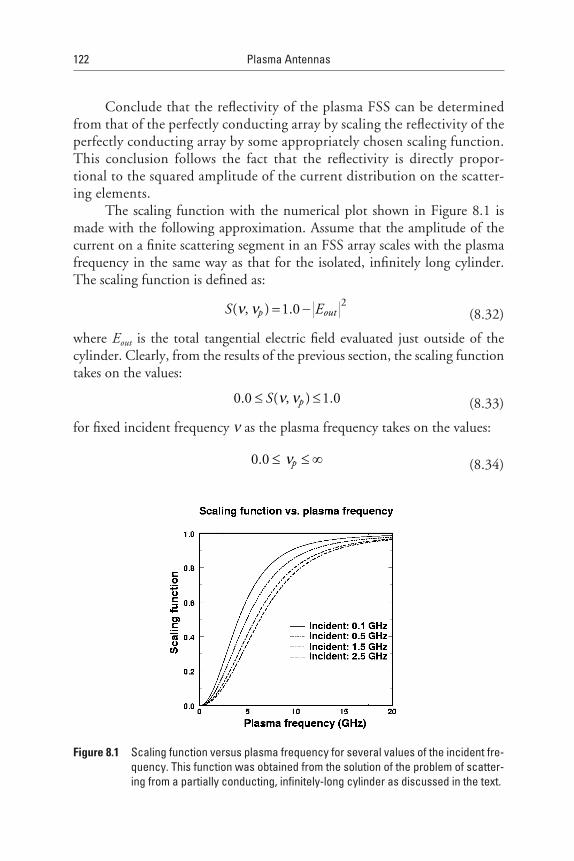
122 PlasmaAntennas
Conclude that the reflectivity of the plasma FSS can be determined from that of the perfectly conducting array by scaling the reflectivity of the perfectly conducting array by some appropriately chosen scaling function. This conclusion follows the fact that the reflectivity is directly propor-tional to the squared amplitude of the current distribution on the scatter-ing elements.
The scaling function with the numerical plot shown in Figure 8.1 is made with the following approximation. Assume that the amplitude of the current on a finite scattering segment in an FSS array scales with the plasma frequency in the same way as that for the isolated, infinitely long cylinder. The scaling function is defined as:
= − 2( , ) 1.0p outS Eν ν (8.32)
where Eout is the total tangential electric field evaluated just outside of the cylinder. Clearly, from the results of the previous section, the scaling function takes on the values:
≤ ≤0.0 ( , ) 1.0pS ν ν (8.33)
for fixed incident frequency n as the plasma frequency takes on the values:
≤ ≤ ∞0.0 pν (8.34)
Figure 8.1 Scalingfunctionversusplasmafrequencyforseveralvaluesoftheincidentfre-quency.Thisfunctionwasobtainedfromthesolutionoftheproblemofscatter-ingfromapartiallyconducting,infinitely-longcylinderasdiscussedinthetext.

PlasmaFrequencySelectiveSurfaces 123
This function is plotted versus np for several values of the incident frequency.
8.3 Results
Two cases are presented: (1) an array designed to have a well-defined reflec-tion resonance near 1 GHz (a bandstop filter), and (2) an array designed to operate as a good reflector for similar frequencies.
8.3.1 Switchable Bandstop Filter
Each scattering element is assumed to be 15 cm in length and 1 cm in diameter. The vertical separation is taken to be 18 cm, while the lateral separation is taken to be 10 cm. The results for the perfectly conducting case, along with those for several values of the plasma frequency, are pre-sented in Figure 8.2. A well-defined reflectivity resonance exists at 1 GHz. This result indicates that appreciable reflection occurs only for plasma fre-quencies above 2.5 GHz. The results of Figure 8.2 illustrate the essence of the plasma FSS: a highly reflective bandstop filter can be achieved and can be switched on and off simply by controlling the properties of the plasma. The results for the perfectly conducting case along with those for several values of the plasma frequency are presented in Figure 8.3. A well-defined reflectivity resonance exists at 1 GHz. This result indicates that appreciable reflection occurs only for plasma frequencies above 2.5 GHz. The results of Figure 8.3 illustrate the essence of the plasma FSS: a highly reflective band stop filter can be achieved with can be switched on and off simply by controlling the properties of the plasma.
Figure 8.2 SchematicrepresentationofanFSSdipolearray.
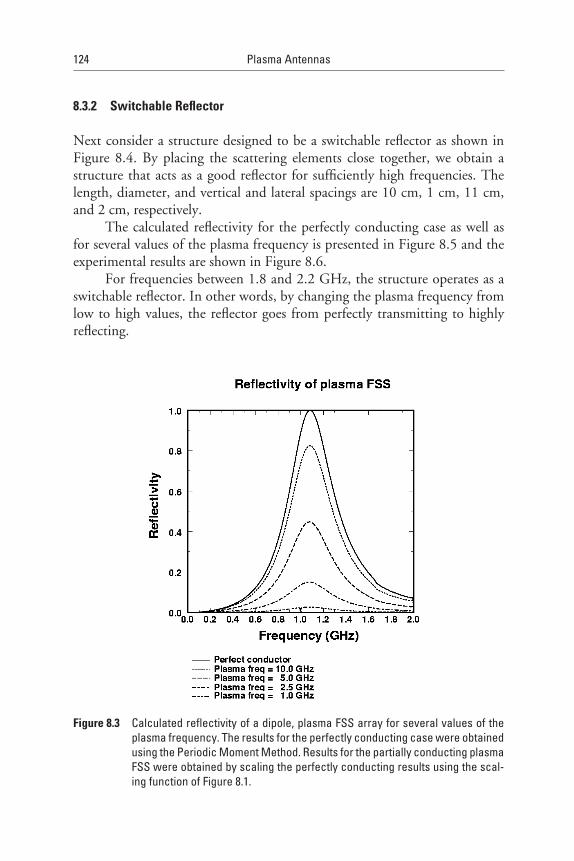
124 PlasmaAntennas
8.3.2 Switchable Reflector
Next consider a structure designed to be a switchable reflector as shown in Figure 8.4. By placing the scattering elements close together, we obtain a structure that acts as a good reflector for sufficiently high frequencies. The length, diameter, and vertical and lateral spacings are 10 cm, 1 cm, 11 cm, and 2 cm, respectively.
The calculated reflectivity for the perfectly conducting case as well as for several values of the plasma frequency is presented in Figure 8.5 and the experimental results are shown in Figure 8.6.
For frequencies between 1.8 and 2.2 GHz, the structure operates as a switchable reflector. In other words, by changing the plasma frequency from low to high values, the reflector goes from perfectly transmitting to highly reflecting.
Reflectivity
Figure 8.3 Calculatedreflectivityofadipole,plasmaFSSarrayforseveralvaluesoftheplasmafrequency.TheresultsfortheperfectlyconductingcasewereobtainedusingthePeriodicMomentMethod.ResultsforthepartiallyconductingplasmaFSSwereobtainedbyscalingtheperfectlyconductingresultsusingthescal-ingfunctionofFigure8.1.

PlasmaFrequencySelectiveSurfaces 125
In this case, the scattering elements are chosen to be 10 cm in length and 1 cm diameter. The vertical spacing is 11 cm, and the horizontal spacing is 2 cm.
The superposition of the experimental and theoretical work is given in Figure 8.7 and shows good agreement. In this comparison of theoretical
Figure 8.5 Reflectivity for switchable plasma reflector illustrated. For frequencies be-tween 1.8 and 2.2 GHz, the structure operates as a good reflector for suffi-cientlyhighvaluesoftheplasmafrequency.
Figure 8.4 Illustration of a switchable reflector. The length, diameter, and vertical andlateralspacingsare10cm,1cm,11cm,and2cm,respectively.
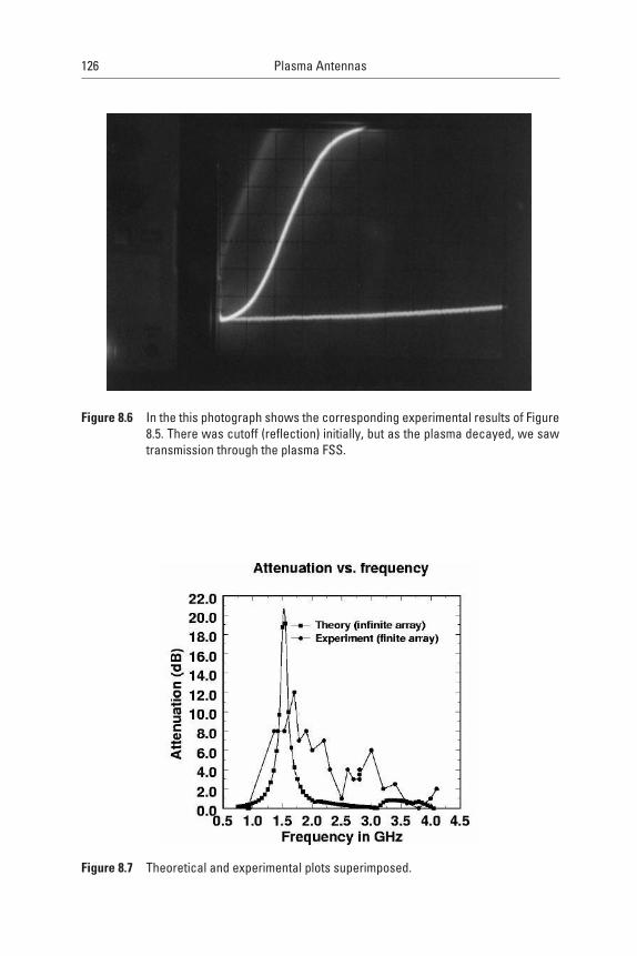
126 PlasmaAntennas
Figure 8.6 InthethisphotographshowsthecorrespondingexperimentalresultsofFigure8.5.Therewascutoff(reflection)initially,butastheplasmadecayed,wesawtransmissionthroughtheplasmaFSS.
Figure 8.7 Theoreticalandexperimentalplotssuperimposed.

PlasmaFrequencySelectiveSurfaces 127
calculations on plasma FSS and the corresponding experiments on plasma FSS for attenuation versus incident frequency, the plasma tubes were 4 and 5 inches long with the metal ends included. The plasma tubes were 2 inches apart horizontally and one inch apart vertically. Differences are due mainly to the fact that the theoretical plot was an infinite array and the experimental plot was a finite array. The peak resonance in the theoretical and experimen-tal plots was very close, and the subpeaks in the experimental are due to the finite size of the array. An alternate to this analysis can be made by using a mutual impedance model found in Kraus and Marhefka [3], which can apply to a finite array. This model can be extended from metal antennas to plasma antennas. Using this model, a matrix for currents in the plasma antennas can be used to derive the radiated antenna field. This approach given here is similar to the approach by Munk [2] on metal FSS.
References
[1] Anderson, T., and I. Alexeff, “Plasma Frequency Selective Surfaces,” IEEETransactionsonPlasmaScience, Vol. 35, No. 2, April 2007, p. 407.
[2] Munk, B. A., FrequencySelectiveSurfaces, New York: Wiley-Interscience, 2000.
[3] Kraus, J., and R. Marhefka, Antennas for All Applications, 3rd ed., New York: McGraw-Hill, 2001, pp. 444–454.

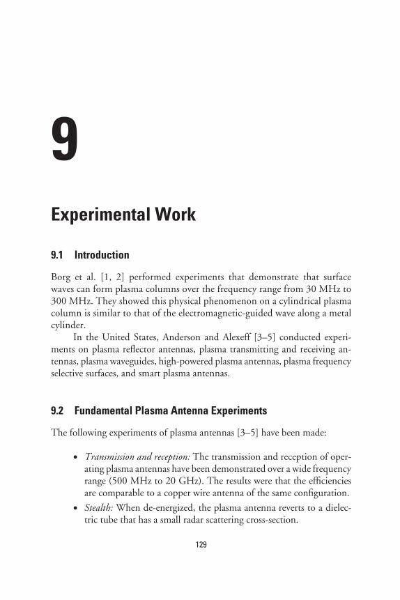
129
9Experimental Work
9.1 Introduction
Borg et al. [1, 2] performed experiments that demonstrate that surface waves can form plasma columns over the frequency range from 30 MHz to 300 MHz. They showed this physical phenomenon on a cylindrical plasma column is similar to that of the electromagnetic-guided wave along a metal cylinder.
In the United States, Anderson and Alexeff [3–5] conducted experi-ments on plasma reflector antennas, plasma transmitting and receiving an-tennas, plasma waveguides, high-powered plasma antennas, plasma frequency selective surfaces, and smart plasma antennas.
9.2 Fundamental Plasma Antenna Experiments
The following experiments of plasma antennas [3–5] have been made:
Transmission and reception: The transmission and reception of oper-ating plasma antennas have been demonstrated over a wide frequency range (500 MHz to 20 GHz). The results were that the efficiencies are comparable to a copper wire antenna of the same configuration.
Stealth: When de-energized, the plasma antenna reverts to a dielec-tric tube that has a small radar scattering cross-section.
·
·

130 PlasmaAntennas
Reconfigurability: At 3 GHz a parabolic plasma reflector has been developed. When energized, it reflects the radio signal. When de-energized, the radio signal passes freely through it.
Shielding: The plasma reflector, when placed over a receiving horn and energized, prevents an unwanted 3-GHz signal from entering. When the antenna is de-energized, the signal passes through freely.
Protection from electronic warfare: When a plasma reflector antenna operates and reflects a signal at 3 GHz, a signal at 20 GHz freely passes through the same reflector. The idea is that a plasma antenna can be so configured that a high-frequency, electronic warfare signal can pass through the antenna without appreciable interaction, while the an-tenna is transmitting and receiving signals at a lower frequency.
Ruggedization and mechanical robustness: In one design, the glass tubes comprising the plasma antenna are encapsulated in a dielectric block. In a second design, the plasma antennas are composed of flex-ible plastic tubes.
Mechanical reconfigurability: An operating plasma antenna composed of flexible plastic tubes has been mechanically manipulated, in par-ticular, a plasma antenna that may be compressed and stowed when not being used.
Plasma waveguides: A coaxial plasma waveguide has been developed. The advantage of such a waveguide is that it reverts to dielectric tubes when de-energized and does not have large radar cross-section.
A coaxial plasma closing switch is shown in Figure 9.1. In this switch, the outer conductor is a metal shell, and the inner conductor is a plasma discharge tube. When the tube was not energized, the outer shell comprises a metal waveguide beyond cutoff, and no radiation is transmitted. When the plasma discharge tube was energized, the apparatus becomes a coaxial wave-guide, and the transmission of radio signals was excellent.
A version of the first plasma antenna is shown in Figure 9.2(a). Under the proper conditions, it was found that the plasma antenna transmitted and received signals virtually identically to a metal antenna in the static mode for the same shape of antennas and frequency. The plasma antenna has the added advantage of reconfigurability.
In Figure 9.2(b) the signal strength was measured by using a panoramic receiving horn antenna. A panoramic receiver is a receiver that can be ad-justed to receive a wide range of frequencies. The received signal strength from a transmitting folded dipole plasma antenna [similar to Figure 9.2(a)]
·
·
·
·
·
·

Experimental Work 131
and a folded metal dipole antenna of the same dimensions are plotted in Figure 9.2(b). This shows that the transmitting plasma antenna is virtually the same as the corresponding metal antenna in the static nonreconfigurable mode. How-ever, many of the advanatages of plasma antennas are in reconfiguration.
An early plasma parabolic reflector antenna is shown in Figure 9.3. With this apparatus, stealth, reconfigurability, and protection from electronic warfare are demonstrated.
The following tests on comparing a plasma reflector antenna and a metal reflector antenna were done at the Malibu Research anechoic cham-ber in 2002. Reflected patterns were measured for a conventional reflector antenna and a plasma tube reflector for performance comparison. In these experiments, the antenna configurations were designed as an offset-fed, cy-lindrical parabolic reflector.
The conventional solid antenna is a parabolic cylinder 28 inches high by 36.5 inches long, with the parabolic shape in the vertical dimension. It is an offset design, with the parabolic segment being the outer 28 inches of a 52-inch diameter dish. The focal distance for the parabola is 13 inches, which yields a 13-inch depth for the parabola at the highest point. The antenna is fed by a line source feed, which is accomplished by the use of a pillbox an-tenna. The pillbox antenna is mounted at the front of the reflector antenna,
Figure 9.1 Coaxialplasmaonaswitch.

132 PlasmaAntennas
Figure 9.2 (a)Earlyplasmaantenna.(b)Signalstrengthofabasicplasmatransmittingfoldeddipole.Antennasimilartotheplasmaantennainpart(a)comparedtothecorre-spondingmetalfoldeddipoleantenna.SignalstrengthisindBm.Theargongasplasmaantennareceivedsignalstrengthisgivenbyacurvewithsolidblackdots.Thecorrespondingmetalantennareceivedsignalstrengthisgivenbyacurvewithsolidblacksquares.Thepanoramichornreceiverwasused.

Experimental Work 133
in the prime focus configuration, and has a flared mouth to provide a nominal –10-dB amplitude taper across the vertical dimension of the reflector. The pillbox feed is itself a parabola in the lengthwise dimension. The focal dis-tance of the pillbox parabola is 9 inches, and the depth of the pillbox includ-ing feed flare is approximately 14 inches. The plate spacing of the feed parallel plates was chosen to allow the resulting horizontal polarization (i.e., the electric field is parallel to the long dimension of the reflector). The frequency of opera-tion for the test was selected to be 3.0 GHz, which is well within the bandwidth of the WR-284 waveguide being used in the design. A photograph of the solid metal reflector antenna is seen in Figure 9.4.
The plasma configuration consists of simply replacing the solid reflec-tor metal surface with a plasma tube configuration having the same nominal shape and dimensions. A photograph of this system is shown in Figure 9.5.
The plasma reflector is comprised of 17 fluorescent light tubes, with a nominal projected tube-to-tube spacing of 1.5 inches. The tube spacing was
Figure 9.3 Earlyplasmareflectorantenna.
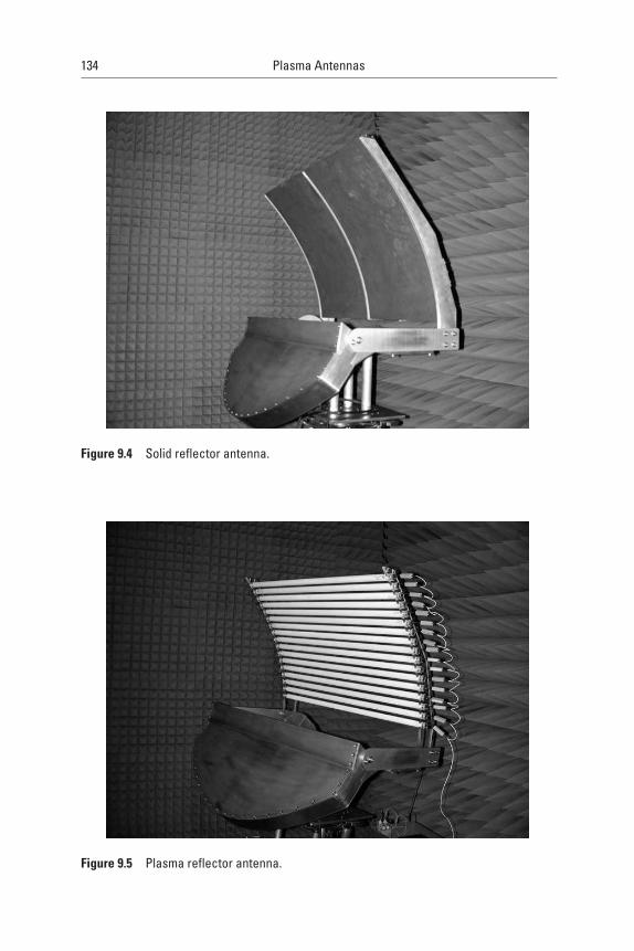
134 PlasmaAntennas
Figure 9.4 Solidreflectorantenna.
Figure 9.5 Plasmareflectorantenna.
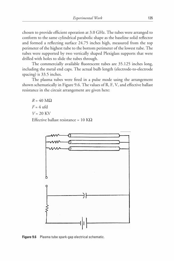
Experimental Work 135
chosen to provide efficient operation at 3.0 GHz. The tubes were arranged to conform to the same cylindrical parabolic shape as the baseline solid reflector and formed a reflecting surface 24.75 inches high, measured from the top perimeter of the highest tube to the bottom perimeter of the lowest tube. The tubes were supported by two vertically shaped Plexiglass supports that were drilled with holes to slide the tubes through.
The commercially available fluorescent tubes are 35.125 inches long, including the metal end caps. The actual bulb length (electrode-to-electrode spacing) is 33.5 inches.
The plasma tubes were fired in a pulse mode using the arrangement shown schematically in Figure 9.6. The values of R, F, V, and effective ballast resistance in the circuit arrangement are given here:
R = 40 MWF = 4 ufd
V = 20 KV
Effective ballast resistance = 10 KW
Figure 9.6 Plasmatubespark-gapelectricalschematic.

136 PlasmaAntennas
Antenna patterns were measured at 3.0 GHz. Sample antenna patterns for the reference solid metal reflector antenna and for the proof-of-principle plasma reflector antenna are plotted together in Figure 9.7. As seen in Fig-ure 9.7, the patterns are a very good match between the proof-of-principle plasma antenna and those of the reference solid conventional antenna.
Figure 9.7 also shows the received signal from the plasma antenna when the tubes are not energized. It is seen that the received signal has dropped by approximately –20 dB. This signal level is primarily due to reflections from the plasma containers and the electrodes. This level could easily be reduced to below the –30-dB level with proper design attention.
Figures 9.7 and 9.8 show that the plasma antenna reflector antenna had lower sidelobes than the corresponding metal reflector antenna. No theory has been done to date to predict this effect, but it may be due to the soft surface effects of the plasma reflective to the metal.
Figure 9.7 Radiationpatterns.

Experimental Work 137
The noise level introduced to the receiver by the plasma reflective sur-face was also measured. The received signal at the output of the antenna was amplified to a level to ensure that the receive system noise was dominant and not the set by the thermal noise of the spectrum analyzer. The noise level was monitored with the signal off and the tubes not energized. The plasma tubes were then energized and the change in noise level was monitored. Noise spikes corresponding to an equivalent temperature increase of approx-imately 400K were observed with each plasma firing. The plasma pulse has a rise time of a few nanoseconds with a long decay time. It was suspected that the rapidly changing current at the onset of the pulse was radiating in the 3.0-GHz region. An experiment was conducted by laying an insulated wire near the feed horn with the same current limiting resister and then letting the spark-gap fire (without energizing the plasma tubes), causing a current pulse to occur. The noise generated and monitored by the spectrum analyzer was very similar to that generated by the plasma tubes. This tended to verify that the noise was generated by the fast rise time nature of the pulse and not the plasma gas.
The spark-gap technique to produce pulsing produced some EMI noise, but the smart plasma antenna did not use a spark-gap technique to produce the pulsing, and no EMI noise was measured.
Reduced sidelobe levelsfor plasma antenna
−40 −40 −30Degrees
−20 −10 0 10 20 30 40
−35
−30
−25
−20
−15
−10
−5
0
Figure 9.8 Plasmaantennareducedsidelobes.

138 PlasmaAntennas
9.3 Suppressing or Eliminating EMI Noise Created by the Spark-Gap Technique
The approach shown in Figure 9.9 applies to the noise generated by the spark-gap technique for pulsing. Techniques that were developed for the smart plasma antenna did not use a spark-gap technique for pulsing and EMI pulser noise was not an issue. EMI noise produced by the pulsing apparatus was greatly reduced or eliminated using these techniques.
In some experiments using the spark-gap-pulsing technique, EMI sig-nals leak into the receiver from the pulser system. By rewiring the pulser and making it electrically symmetric to the ground, the pulsed noise source is converted from a monopole to a multipole and the EMI noise from spark-gap pulsing is greatly reduced. At the most sensitive panoramic receiver set-ting, the pulser noise is comparable to thermal noise. Figure 9.10 shows the
+10 KV
+10 KV
Spark gap
Plasma tube (6)
Spark gap
10 F−9
1 MΩ
1 MΩ
10 F−9
Plasma tube (6)
1 MΩ
Symmetric less-noisy setup
Previous noisy setup
Noise reduction
Figure 9.9 Circuitdiagramswithplasmaantennasforsuppressingpulsernoise.

Experimental Work 139
Figure 9.10 Signalwithpulseroff.
Figure 9.11 Signalwithpulseronwithnoisereduction.

140 PlasmaAntennas
oscilloscope signal with the pulser off, and Figure 9.11 shows the oscilloscope signal with the pulser on showing noise reduction.
9.4 Conclusions on the Plasma Reflector Antenna
The performance of the proof-of-principle plasma antenna was excellent when compared to the solid reflector. The measured patterns and gain were very similar between the two configurations. The stealth nature of this antenna approach can be easily recognized as the antenna essentially disappears to a radar signal when the tubes are not energized. A reduction of –20 dB was demonstrated, which can easily be reduced to less than –30 dB with careful design. These measured results are outstanding considering that the plasma reflector design was restricted to tubes that were commercially available. This plasma antenna was used in a high-current, short-pulse configuration. For stealth projects, the first metal reflector could be encased inside the body of a structure.
9.5 Plasma Waveguides
A second, antenna-related plasma application is a plasma waveguide [6, 7], as shown in Figure 9.12. Here an inner conductor comprises one plasma tube surrounded by an outer shell of eight plasma tubes.
When the gas is excited into a plasma, the structure transmits radiation almost as well as a coaxial cable, but when it is off, the transmitted signal decreases by over 100 dB—a factor of 1010. Such plasma waveguides could convey radiation to the antennas on the mast of a ship, yet become transpar-ent to radiation when de-energized.
Figures 9.13 and 9.14 are schematics of two types of plasma waveguide designs. When the plasma in the inner tube is on, electromagnetic waves propagate down the waveguide. When the inner plasma tube is turned off, the waveguide is below cutoff and no propagation occurs.
The inner cylinder is filled with plasma (darkened area), and the outer annular ring is filled with plasma. A nonconducting region (white) is in be-tween the inner cylinder and outer cylindrical annular ring. The plasma skin depth is reconfigurable creating a reconfigurable waveguide. Radar signals would pass through a de-energized waveguide rather than be reflected. In fact, these waveguides could pass in front of operating antennas and be virtu-ally invisible when off.

Experimental Work 141
9.6 Plasma Frequency Selective Surfaces
For more material on plasma frequency selective surfaces, refer to Chapter 8. A third plasma antenna application is reconfigurability. The effects of a re-configurable plasma frequency selective surface (FSS) filter are shown in Fig-ure 9.15.
Putting a plasma FSS between a transmitter and a receiver removes the second and higher harmonics (2 dB per square). In the first oscilloscope trace, we observe several spectral lines emitted from an oscillator driven to a nonlinear
Figure 9.12 Plasmawaveguide.
Figure 9.13 Aninsideplasmatubeinametalorplasmawaveguide.

142 PlasmaAntennas
Figure 9.14 Asecondplasmawaveguidedesign.
Figure 9.15 Plasma frequency selective surface (FSS) filter removes the second andhigherharmonics.

Experimental Work 143
limit. In the second oscilloscope trace, several of the higher-frequency lines have been removed by energizing a plasma FSS filter placed between the transmitter and the receiver. Figures 9.16 and 9.17 are photographs of the plasma FSS setup.
Figure 9.16 Photographof the labsetupshowing thebuiltplasmaFSSwithdipoleele-mentsandthehornreceiverantenna.
Figure 9.17 Close-upphotoofanexperimentalsetupplasmaFSSwithdipoleelements.
144 PlasmaAntennas
9.7 Pulsing Technique
Plasma tubes can be ionized by DC. However, if the tubes are ionized by extremely short bursts of DC, the following remarkable improvements can be made. The plasma is produced in an extremely short time: -2 ms, but the plasma persists for a much longer time, 1/100 second. This is the reason why fluorescent lamps can operate on 60-Hz or 50-Hz electric power. Conse-quently, if the pulsing rate is increased to 1 kHz, the tubes are operating at an essentially constant density.
There are three benefits to this new mode of operation.
1. The exciting current is on for only 2 ms, while it is off for 1 ms. Therefore, the discharge current is only on for 0.2% of the time, so current-driven instabilities are not present for most of the time. However, the current-driven instabilities have proven to not be a problem. In general, operating the plasma tubes in the noncurrent-carrying, afterglow state should produce considerably less noise than in operating in the current-carrying state. Even in the current-driven state, we have found that the thermal noise in the plasma antenna is less than that of that of a metal antenna. This is true for frequencies above 1 GHz for a fluorescent tube and for lower fre-quencies if the pressure is reduced.
2. Unexpectedly, the plasma density produced by the pulsed-power technique is considerably higher than the plasma density produced by the same power supplied in the steady-state. This observation produces two beneficial results. The plasma antenna can operate at much higher plasma frequencies and densities than before in the steady-state without destroying the discharge tube electrodes. Formerly, using commercial fluorescent tubes, we were limited to steady-state operation below 800 MHz. Now several gigahertz can be operated. The upper frequency limit has not been explored.
3. The plasma antennas can operate at much higher plasma frequen-cies and densities using lower average consumption. This results in much lower power consumption.
One of the remarkable plasma effects experimentally discovered is the large increase in plasma density at the same average power input provided by pulsing the power input [8–12]. In these experiments, a density increase of over 100 has been observed. Although various experimenters have observed

Experimental Work 145
similar effects using different power input techniques, to our knowledge no one has provided a theoretical explanation as of yet.
Since the power [13] is obviously being deposited into the plasma, we assume that during the power input, an enhanced plasma loss occurs [private communication with I. Alexeff, 2007]. This plasma loss occurs on a time scale T1. By turning off the power input, this plasma loss process disappears on a time scale T2. The resulting afterglow plasma disappears on a much slower time scale T3. We model this as a system driven by a power delta function repeating on a time period T4. The height of the delta function is proportional to T4, so the longer the time between pulses, the higher the delta function, but the average power input is preserved.
As a first approximation on a single pulse basis, we obtain
= −
2 4
1 5expAG
SS
N T TN T T
(9.1)
where NAG is the afterglow density during pulsing and Nss is the density dur-ing steady-state operation. In our experiments, T4 is about 1,000 times T5 (the duration of the delta function). If we assume that the fast decay process T1 is of the same approximate length as the time in which this decay process disappears on T2, this calculation yields a density enhancement of about 300. This number agrees with our observed density enhancement. This calcula-tion ignores the plasma left over from the preceding pulse, but most of this is dumped by the effects of the pulse. In any case, it can only improve plasma density conditions.
Plasma tubes(12 total)
Spark gap
10−
1.5 * 10 6 ohm
Fan toextinguish arc
Figure 9.18 Earlypulsingapparatus.

146 PlasmaAntennas
Figure 9.18 is a schematic of our pulsing apparatus. A 0–30-KV sup-ply is connected to an RC supply comprising a 1.5-MW resistor feeding a nanofarad capacitor.
The resultant high-voltage arc over a spark gap provided a pulsed cur-rent to the fluorescent lamps, up to 12 wired in series. When operating arc high pulsing frequencies—1 kHz and up—the spark gap tends to go over to a steady-state arc. A small blower has been placed on the spark gap to flush out the ionized air. In practice, this solution works very well.
Figure 9.19 shows the pulsing plasma tubes and the receiving horn.In conclusion, the recent inclusion of a pulsed power supply for the
plasma tubes provides reduced noise, higher steady-state DC plasma density, and reduced power consumption.
9.8 Plasma Antenna Nesting Experiment
This section is related but different to the plasma antenna nesting experiment from Section 5.5. Figure 9.18 is similar to Figure 5.6, but different because the lower frequency in Section 9.8 is less than the lower frequency in Section 5.5.
Figure 9.19 Pulsingplasmatubesandreceivinghorn.
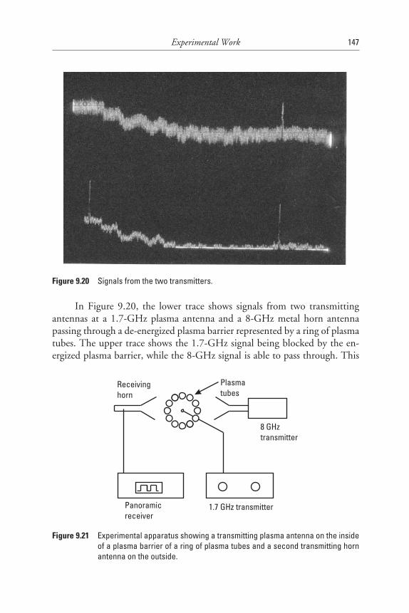
Experimental Work 147
In Figure 9.20, the lower trace shows signals from two transmitting antennas at a 1.7-GHz plasma antenna and a 8-GHz metal horn antenna passing through a de-energized plasma barrier represented by a ring of plasma tubes. The upper trace shows the 1.7-GHz signal being blocked by the en-ergized plasma barrier, while the 8-GHz signal is able to pass through. This
Figure 9.20 Signalsfromthetwotransmitters.
Panoramicreceiver
1.7 GHz transmitter
Receivinghorn
8 GHztransmitter
Plasmatubes
Figure 9.21 Experimentalapparatusshowingatransmittingplasmaantennaontheinsideofaplasmabarrierofaringofplasmatubesandasecondtransmittinghornantennaontheoutside.

148 PlasmaAntennas
means that the energized plasma barrier has a plasma frequency that is greater than 1.7 GHz but less than 8 GHz.
The received signal with the plasma on shows considerably more noise than that with the plasma off. The noise signal apparently is not present on the microwave signal, but is due primarily to receiver pickup via the power line. Disconnecting the receiving antenna from the panoramic receiver does not change the observed noise level.
In Figure 9.21 a plasma transmitting antenna is placed inside a ring of plasma tubes acting as a barrier. A second transmitting horn antenna is placed outside the ring of plasma tubes. The two signals are received by a receiving horn antenna outside the ring of plasma tubes when the plasma frequency in these tubes is below 1.7 GHz or turned off.
9.9 High-Power Plasma Antennas
9.9.1 Introduction
The objective is to operate plasma antennas at high power. Plasma antennas have been successfully operated at over 2 MW in the pulsed mode. There is a simple technique of increasing the output power of the pulsed system by factors of 2 in an extremely simple fashion. This development may be of great use in electronic warfare.
9.9.2 The High-Power Problem
Consider a high-voltage system charging a coaxial cable. A spark gap connects this coaxial cable to another coaxial cable terminating in an antenna. A photo of such a cable system is shown in Figure 9.22. This system has been observed to radiate pulsed energy at over 2 MW. The apparatus used is shown in Fig-ure 9.23. The problem is that, in general, the power supply is voltage limited by spark-overs. The coaxial cable system, on the other hand, can stand enor-mous voltages on a short time basis.
One way around the power supply voltage limitation is to charge a very low impedance line. The low impedance line discharges through a spark gap into a line with a tapered impedance. For example, if the line corre-sponds to an impedance of 10 ohms, and the line increases in impedance to 300 ohms, which matches the antenna to space, the voltage rises by a factor of
300/10, and the power rises by a factor of 30 over that if the 300-ohm line were charged directly by the power supply. Such a tapered line has been used
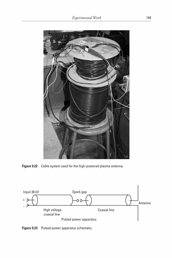
Experimental Work 149
Figure 9.22 Cablesystemusedforthehigh-poweredplasmaantenna.
Input 30 kV
Antenna
Spark gap
High voltagecoaxial line
Pulsed power apparatus
Coaxial line−
+
Figure 9.23 Pulsedpowerapparatusschematic.
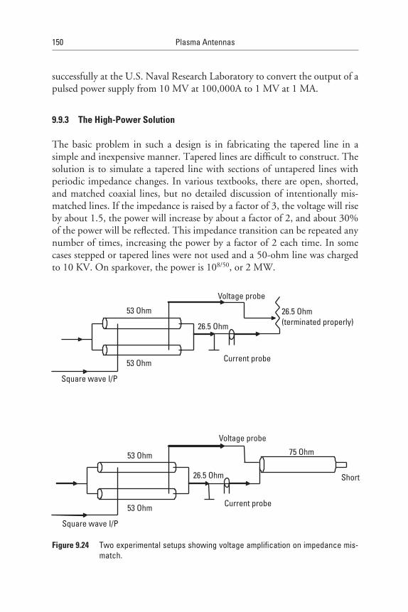
150 PlasmaAntennas
successfully at the U.S. Naval Research Laboratory to convert the output of a pulsed power supply from 10 MV at 100,000A to 1 MV at 1 MA.
9.9.3 The High-Power Solution
The basic problem in such a design is in fabricating the tapered line in a simple and inexpensive manner. Tapered lines are difficult to construct. The solution is to simulate a tapered line with sections of untapered lines with periodic impedance changes. In various textbooks, there are open, shorted, and matched coaxial lines, but no detailed discussion of intentionally mis-matched lines. If the impedance is raised by a factor of 3, the voltage will rise by about 1.5, the power will increase by about a factor of 2, and about 30% of the power will be reflected. This impedance transition can be repeated any number of times, increasing the power by a factor of 2 each time. In some cases stepped or tapered lines were not used and a 50-ohm line was charged to 10 KV. On sparkover, the power is 108/50, or 2 MW.
Square wave I/P
Square wave I/P
53 Ohm
53 Ohm
53 Ohm
53 Ohm
Current probe
Current probe
26.5 Ohm
26.5 Ohm
Voltage probe
Voltage probe
75 Ohm
26.5 Ohm(terminated properly)
Short
Figure 9.24 Twoexperimentalsetupsshowingvoltageamplificationonimpedancemis-match.

Experimental Work 151
9.9.4 Experimental Confirmation
This apparatus was fabricated as shown in Figure 9.24, in which two 53-ohm lines are connected in parallel, yielding a 25.5-ohm line. This line is con-nected to a 75-ohm line, yielding the 3:1 desired mismatch. The lines are driven by a pulser on a Tektronix oscilloscope. The lines are very long, about 100 meters in length, which sufficiently slows down the phenomenon that it can be observed on a conventional oscilloscope.
Experimental data are shown in Figures 9.25 and 9.26. In Figure 9.25 the 25.5 compound line is terminated by a potentiometer, which is adjusted to properly terminate the line, as observed by minimal reflections. The termi-nation value was measured by an ohm-meter to be the desired value of about 25 ohms. The voltage (bottom trace) rises by about 2 squares, while the cur-rent (top trace) also rises by about 2 squares.
Then the potentiometer is replaced by the 75-ohm line. The voltage, as expected, rises to about 3 squares, while the current declines to about 1 square. Thus, the power through the 75-ohm line is now double what it would have been if excited directly by the power supply. This is accomplished with a little power loss.
The schematic of the high power plasma antenna is given in Figure 9.27.
Figure 9.25 The25.5compoundlineterminatedbyapotentiometer.

152 PlasmaAntennas
9.9.5 Conclusions on High-Power Plasma Antennas
9.9.5.1 High-PowerOperationofPlasmaAntenna
A coaxial cable was charged to 25 KV. It was discharged through a spark gap into a second coaxial cable coupled to a plasma antenna. The radiation was
Figure 9.26 Thepotentiometerreplacedbythe75-ohmline.
25 KV
1 Mega Ohm
Coaxial cable
Plasma tubes
Comparativemetalantenna
Pulse power unit - 2.5 MW
Figure 9.27 Schematicofhighpowerplasmaantenna.Ifthepulsedpowerrepetitionrateishighenough,theplasmadensityismaintainedfrompulsetopulse.

Experimental Work 153
picked up on a panoramic receiver or an oscilloscope. A comparison of the plasma antenna with the metal antenna was performed. The received signals were comparable. The calibration of the power output was done by feeding the metal antenna with a local oscillator. The power received from the previ-ous step was compared with that of the pulsed power supply, verifying that the pulsed power output was 2.5 MW.
A simple way of arbitrarily increasing the power in a pulsed power sys-tem has been demonstrated, using only conventional coaxial lines. This is a significant advance in pulse-power technology, and this technique in further experiments will be used on plasma antennas. There is an increase of trans-mitted power and loss of efficiency as the number of feed cables connecting to the terminating cable is increased. Each feed cable is assumed to have the same impedance as the terminating cable.
A 2-MW pulsed power supply was tested on a plasma antenna. In the transmitting mode, the plasma antenna was as efficient as a metal antenna for high power. The plasma antenna has the added advantages of reconfigurability, which a metal antenna does not have. This reconfirms what was found for lower powers. A megawatt power supply was tested on a plasma antenna. A pulsed power supply similar to the one used at the Naval Research Laboratory was used to generate megawatt radiation pulses with metal antennas. The design of the apparatus is shown in Figure 9.27. A section of the 50-ohm coaxial cable is charged to 25 kV. It then discharges through a spark gap into a second section of coaxial cable and then into four fluorescent lamps connected in series, form-ing a loop antenna. Previous experiments have shown that if the pulse repetition rate is over a kilohertz, the plasma in the fluorescent lamps is in essentially the steady-state. The pulse of microwave radiation entering the plasma antenna ra-diates and is received on a small wire antenna about 1 meter away. The received signal is about 5 volts in amplitude. Since the input impedance of the antenna is 50 ohms, as determined by terminating resistors, the received power is 0.5 watt. The frequency of the radiation is about 13 MHz, in approximate agreement with the Naval Research Laboratory results with metal antennas. To calibrate the power output from the transmitter, the plasma antenna was replaced with a wire loop antenna of the same physical dimensions. The received power from the pulsed power transmitter was the same as for the plasma antenna. The wire antenna was disconnected from the pulsed power supply and was connected to a 10-MHz transmitter, and the received power on a panoramic receiver was mea-sured. The transmitter was connected directly into the panoramic receiver, the signal strength to the previous value was adjusted, and the attenuation needed to do so was recorded. The attenuation required was 70 dB. If the power received is multiplied from the pulsed power supply via the plasma antenna by 70 dB, the

154 PlasmaAntennas
radiated power from the plasma antenna is 5 MW. This result is in agreement with the measured radiation output from the Naval Research Laboratory, except that they used a metal antenna in a plasma antenna. The power output from the pulsed plasma antenna was impressive. A handheld fluorescent lamp was used and illuminated by radiation from the pulsed power supply. The radiation does not ignite the fluorescent lamps unless they are preignited. In addition, there was an attempt to calibrate the plasma antenna by coupling in radiation from a 10-MHz oscillator. The oscillator was immediately destroyed, a result that would be expected for electronic warfare.
9.10 Basic Plasma Density and Plasma Frequency Measurements
Plasma density can be estimated experimentally by the reflection and trans-mission of electromagnetic waves in scattering from plasma. Please review Chapter 2 for the derivation of reflection and transmission coefficients of electromagnetic waves impinging on plasma as a function of plasma density or plasma frequency.
One plasma tube of the smart plasma antenna successfully blocked satel-lite frequencies in a DIRECTV system, as seen in Figure 9.28. The same energy was used in this experiment as in the operation of the smart plasma antenna. This means that the plasma frequency in the smart plasma antenna operation in the on mode was higher than the satellite frequencies used by DIRECTV.
The plasma reflector antenna in Figure 9.5 reflected a 3-GHz signal, in-dicating that the plasma frequency in this experiment is greater than 3 GHz, as indicated in Figure 9.7.
9.11 Plasma Density Plasma Frequency Measurements with a Microwave Interferometer and Preionization
A Ku-band (12.4 to 18 GHz) microwave interferometer was constructed and put into operation and measured the plasma density of several commercial plasma tubes [private communication with L. Barnett, 2004]. A high-power pulse modulator and S-band magnetron with a WR284 waveguide measure-ment system was put into operation. A plasma tube was placed into a WR284 waveguide. The first observations made are applicable to the reconfigurability aspect.
The interferometer measured the time variation of plasma frequency/density of a test plasma tube. It is a quality instrument that can accurately

Experimental Work 155
measure phase shifts to at least 0.5° and can operate over a range of approxi-mately 12 to 18 GHz with a tunable YIG oscillator. It utilizes two small antenna probes approximately 5 mm long placed on each side of a plasma column, a precision calibrated phase shifter in the reference leg.
A 40-dB isolator for minimal interaction was placed between the legs and YIG microwave source. A double-balanced mixer for 12- to 18-GHz in-put to the RF and LO ports was used with DC to 3-GHz IF output range to detect the phase and be read by an oscilloscope. The legs of the interferometer had long WR62 waveguide sections to prevent S-band pulse signals from entering and interfering with the measurements.
This was a high-quality 12- to 18-GHz microwave interferometer in the Ku-band waveguide. It has its own built-in YIG tunable source, isolators, calibrated phase shifter, mixer, and so forth. It should be capable of measur-ing a fraction of a degree of phase shift from a small thickness (e.g., 1 cm) plasma and of accurately measuring plasma density from 3 to 18 GHz in both high-speed pulsed (the mixer has a DC to 3-GHz bandwidth, output) and DC plasma discharges.
Figure 9.28 Onetubeof thesmartplasmaantennawasplaced in frontof thehornre-ceiverantenna inaDIRECTVsatellite frequency.Thesatellite frequenciesweresuccessfullyblocked,indicatingthattheplasmafrequencyinthesmartantenna plasma tubes was greater than the satellite frequencies used byDIRECTV.
156 PlasmaAntennas
Both legs of the interferometer were balanced so that approximately equal amounts of waveguide and coaxial line are in each leg to reduce phase noise and drift contributions from the YIG source.
While the instantaneous phase shift can be read directly from the oscilloscope during a plasma pulse, the oscilloscope phase shift can be accurately measured by the precision phase shifter during the pulse by comparing the phases of points of the respective pulse waveform. This compensates for possible varying levels of attenuation through the plasma path during a pulse. The first operation of the interferometer on a plasma tube was to place the probes on each side of the glass tube of a commercial 25-W compact fluorescent lamp (CFL) of approximately 1-cm ID tube diameter. A nominal 6° phase shift was obtained that was modulated by the 40-kHz lamp driver oscillator and the 120 Hz of a full wave rectifier that produces the DC for the oscillator. This produced approximately 6° of average phase shift. The 40-kHz modulation is approximately 3° peak to peak; 6° of plasma phase shift at 14.64 GHz represents a 3.8-GHz plasma frequency.
After an extended warm-up time (1 hour), the phase shift increased to 10°, corresponding to a plasma frequency of 4.8 GHz. The calculations are based on a simple plasma theoretical phase shift in an infinite plasma. The finite tube diameter may have an effect on the measurement; however, simple tests indicate that most of the coupling between the probes is via the plasma path, so we believe the calculation is reasonable—but should be considered as an approximate measure of the plasma frequency and density. Finding that existing commercial CFL plasma tubes with plasma densities potentially already high enough for an S-band microwave antenna, which require only a few tens of watts of CW ionization power in 40-inch tube lengths and have lifetimes of 20,000 hours or more, gave encouragement that very high plasma density tubes can readily be made that will operate in the CW mode necessary for a receive application to be 10 GHz or even higher and have thousands of hours of lifetime.
The S-band modulator system with a pulse S-band magnetron is now in operation and can initially produce pulses at 2.88 GHz up to 134 kW in a WR284 measurement system with directional couplers to measure forward, reflected, and transmitted power. The system should be capable of at least 300 kW, but a bad reverse voltage suppression rectifier on the thyratron lim-its the voltage.
A straight folded 13-W, approximately 23-cm-long CFL tube has been put into the WR284 waveguide and pulse microwave power applied at 2.88 GHz. At approximately 2-ms pulse width and low duty (e.g., 10 pps),

Experimental Work 157
the tube does not self-ionize up to approximately 75 kW. Above approxi-mately 100 kW, the tube self-ionizes quickly (e.g., a submicrosecond) and the RF is highly reflected. In the 75- to 100-kW range, the self-ionization is erratic and can occur at random times in the pulse and is duty dependent. With a shorter pulse width of 0.4 ms, the tube will not ionize at 100 kW up to 40 pps. With a low level of externally applied preionization power (just enough to barely keep the CFL continuously ionized), RF pulse power at all levels in the range of 50–100 kW reflects. While the plasma density is not measured yet, with simultaneously pulsed RF it is most likely that the plasma frequency of the preionization is well below 2.88 GHz and the RF pulse quickly raises (probably in nanoseconds) the plasma density to the level to reflect the 2.88-GHz pulse.
The applied power to the plasma tube in the WR284 waveguide cor-responds to power densities at typical antenna reflector surfaces for many tens of megawatts of radar power (depending on the size of the reflector, of course). While further quantification is required, this does demonstrate that it is possible for unexcited plasma tubes to not be excited by the high power RF pulses of a typical radar operating even up to megawatt levels, and that the same tubes can easily be preionized to reflect a pulse when needed.
At powers under approximately 75 to 100 kW at 2.88 GHz, no preion-ization, the plasma tube does not self-ionize or reflect the RF in a 2-mS pulse, 40 pps. Above approximately 100 kW, the tube self-ionizes in approximately 100–200 ns and reflects the pulse. With the lowest level of externally applied preionization that can be applied and keep the tube barely lit, the HP RF pulses easily ionize (very fast, a submicrosecond) and reflect. A circulator was added to the magnetron output to prevent reflection from getting back to the magnetron and produced quantitative data and photos.
The 100 kW in a WR284 waveguide represents a power density cor-responding to many tens of megawatts of radar power at the surface of a typical radar reflector. This showed that self-ionization will not be a serious problem and possibly that a low power level of preionization is all that is need to select particular tubes to reflect (at least on transmit mode—the receive-only mode will need high-power preionization, of course—that has already been seen up to 5-GHz CW interferometer measured plasma density and can go higher). The CFL tube was mounted in the HP wave-guide. A variable low-frequency ionization power was applied to the tube, from 0% to about 200% rated tube power, and applied some simultaneous ionization. The GE straight compact fluorescent lamps (CFL) were used. One was put in the waveguide, via a hole with RF chokes (to keep the RF in), to get the interferometer on it and obtain a reflection versus a plasma

158 PlasmaAntennas
frequency plot at 2.88 GHz and up to 134 kW. A stable 134-kW pulse RF output was measured at 2.88 GHz with a magnetron. Up to at least 300 kW with this modulator was expected, but there was a damaged rectifier in the modulator that prevented going higher in power (causes the application of a high reverse voltage on the thyratron that causes a reverse breakdown at a higher voltage). This produced more power than originally wanted (60 kW). Since the experiments were done with small plasma tubes of plasma fre-quency in the 1- to 10-GHz range, experiments were done with a couple of 1-cm-long vertical probes spaced at 2 cm, and the transmitted signal at approximately 12 GHz was measured. A 1-cm diameter metal cylinder with an axis vertical was put between them, and the signal decreased by more than 13 dB. This shows that the plasma frequency can readily measured
Figure 9.29 Reflection experiments at 4.6 Torr. A negative polarity microwave detectorwasusedsothatthemaximumreflectionisatthebottomofthescreenwithzeroatthetop.Inthesereflectiontestphotos100%refectionisthreedivisionsfromthebottomscopelineand0%reflectionisgivenatthetopofthetraceat2.0divisionsfromthetop.Thehigh-voltageexcitationpulseisinthefirst2mssotheplasmadensityisessentiallyconstantinthefirst0.5to2msanddeclinesafterwards.Noresonanceisobservedatthispressure.

Experimental Work 159
in a small tube, as most of the signal goes from one probe to the other and passes through a 1-cm-wide space. When a 1-cm or wider plasma becomes conducting to the RF (e.g., plasma frequency exceeding the RF), the signal will be highly attenuated. The time evolution of plasma density to pulse cur-rent and microwave pulses were measured. At 12 GHz waveguide sections can be used as cutoff filters to prevent high-power 3 GHz from entering the interferometer system.
9.11.1 Experiments on the Reflection in the S-Band Waveguide at 3.0 GHz with High Purity Argon Plasma
This section concerns the reflection in the S-band waveguide at 3.0 GHz with high purity argon plasma [private communication with L. Barnett, 2004] (see Figures 9.29 through 9.34). A negative polarity microwave detector was
Figure 9.30 Reflectionexperimentsat3.4Torr.ThepressureisdifferentfromthepressureusedformeasurementsasshowninFigure9.29,butotherconditionsandscalesarethesame.Aresonance(thedipshowsincreasedreflection)isobservedatthispressure.

160 PlasmaAntennas
used so that the maximum reflection is at the bottom of the screen with zero at the top.
In these reflection test photos 100% RF refection from the plasma is three divisions from the bottom scope line and 0% RF reflection from the plasma is given at the top of the trace at 2.0 divisions from top. The high-voltage excitation pulse is in the first 2 ms, so the plasma is essentially con-stant in the first 0.5 to 2 ms and declines afterwards. The pure argon plasma does not persist nearly as long as the mercury plasmas of previous tests, but the argon shows resonance and low noise figure, which was much less than that for mercury. Note the absence resonance at a high pressure of 4.6 Torr. The resonance peak becomes more pronounced up to 380 mTorr and then becomes less pronounced as the pressure decreases to 80 mTorr. The reflec-tion falls off much faster (than the 4.6 Torr case that does not show reso-
Figure 9.31 Reflectionexperimentsat2.0Torr.Thepressureisdifferentfromthepressureusedformeasurementsasshownintheotherfiguresintheset(Figures9.29–9.34),butotherconditionsandscalesarethesame.Aresonance(dipshowsincreased reflection) is observed at this pressure and is more pronouncedthantheresonanceat3.4Torr.

Experimental Work 161
nance) after a resonance, even though there is still significant plasma, just no reflection when the applied RF is above the plasma frequency when there is a clear plasma resonance. There is always some reflection when the plasma fre-quency is above the RF. The maximum peak reflection with the 380-mTorr plasma is approximately 90% as compared to a solid metal pin reflector. Figure 9.29 shows essentially no resonance, and Figures 9.30 and 9.31 show a relatively weak resonance. Interferometer measurements were not made, but from the photos and previous experience the peak plasma frequency is estimated to be in the 4–6-GHz range in Figures 9.32 through 9.34 that show strong resonance. A small diameter tube with approximately 1-cm di-ameter plasma was used. These reflection tests are with a 10-inch homemade tube with variable pressure high purity argon in the S-band waveguide at a 3.00-GHz source and a 3-GHz, 0.4-GHz bandwidth interdigital filter.
Figure 9.32 Reflectionexperimentsat1.1Torr.Thepressureisdifferentfromthepressureusedformeasurementsasshownintheotherfiguresintheset(Figures9.29–9.34),butotherconditionsandscalesarethesame.Aresonance(dipshowsincreased reflection) is observed at this pressure and is more pronouncedthantheresonanceat2.0Torr.
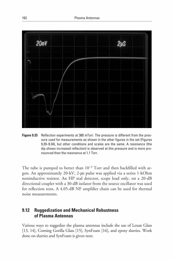
162 PlasmaAntennas
The tube is pumped to better than 10-3 Torr and then backfilled with ar-gon. An approximately 20-kV, 2-ms pulse was applied via a series 1-kOhm noninductive resistor. An HP xtal detector, scope load only, on a 20-dB directional coupler with a 30-dB isolator from the source oscillator was used for reflection tests. A 4.05-dB NF amplifier chain can be used for thermal noise measurements.
9.12 Ruggedization and Mechanical Robustness of Plasma Antennas
Various ways to ruggedize the plasma antennas include the use of Lexan Glass [13, 14], Corning Gorilla Glass [15], SynFoam [16], and epoxy slurries. Work done on slurries and SynFoam is given next.
Figure 9.33 Reflectionexperimentsat380mTorr.Thepressureisdifferentfromthepres-sureusedformeasurementsasshownintheotherfiguresintheset(Figures9.29–9.34), but other conditions and scales are the same. A resonance (thedipshowsincreasedreflection)isobservedatthispressureandismorepro-nouncedthantheresonanceat1.1Torr.

Experimental Work 163
9.12.1 Embedded Plasma Antenna in Sandstone Slurry
The plasma U-shaped antenna in Figure 9.35 was embedded in a sandstone epoxy slurry that solidified. This embedded antenna transmits and receives quite well and has survived several years of hard treatment.
9.12.2 Embedded Plasma Antenna in SynFoam
The plasma tubes have been housed in a strong, lightweight synthetic foam called SynFoam (see Figure 9.36) made by the Utility Development Cor-poration [16]; this foam can be molded into various shapes. SynFoam is a high-performance syntactic foam combining high strength, heat resistance, and light weight with very low moisture absorption. SynFoam’s syntactic
Figure 9.34 Reflectionexperimentsat80mTorr.Thepressureisdifferentfromthepres-sureusedformeasurementsasshownintheotherfiguresintheset(Figures9.29–9.34),butotherconditionsandscalesarethesame.Aresonance(thedipshowsan increasedreflection) isobservedat thispressureand is lesspro-nouncedthantheresonanceat380mTorr.

164 PlasmaAntennas
foam products feature a density of less than 20 pcf and a compressive strength greater than 2,000 psi. The index of refraction of the SynFoam is nearly 1, so it is transparent to RF signals.
Work is currently being done to house the plasma antenna directly in the SynFoam without using glass tubes at all. If this succeeds, a great deal of progress will be done to ruggedize plasma antennas.
Figure 9.35 Embeddedplasmaantennainasandstoneepoxyslurrythatsolidified.Notethatthereflectionoflightfromtheglasstubecontainingtheplasmagivesametallicappearancebutitisglass.
Figure 9.36 SynFoamhousingforplasmatubes.Experimentsareplannedusingthecavi-ties in the SynFoam to directly house the plasma gas without using glasstubesatall.

Experimental Work 165
9.12.2.1 SynFoamTransmissionandReflectionExperiments
Initial tests have been done on SynFoam (shown in Figures 9.37 through 9.41) in regard to plasma antennas. SynFoam has been found to be transparent to RF radiation and it can be ignored in RF reception and transmission characteris-tics. This is shown in Figures 9.37 through 9.41. SynFoam can have a radome support structure, which is durable, lightweight, and inexpensive.
9.12.2.2 IndexofRefractionMeasurementsofSynFoam
The index or refraction of SynFoam was measured at 4.02 GHz as follows. The microwave signal was emitted from a microwave horn and passed through a SynFoam slab 6.5 inches thick, was reflected from a metal plate and passed back through the SynFoam, reentered the microwave horn, was extracted by a directional coupler, and was observed on a panoramic receiver. As a metal plate was moved back and forth, interference occurred on the received signal. The SynFoam slab was rotated, essentially increasing the distance that the mi-crowaves passed through the slab. When the slab was rotated to 45°, there was a minimum in the received signal. This indicated that a microwave signal was retarded by a half-wavelength during its two passages through the SynFoam.
Figure 9.37 SetupofSynFoamtomeasuretheindexofrefractionbymeasuringthephaseshift.
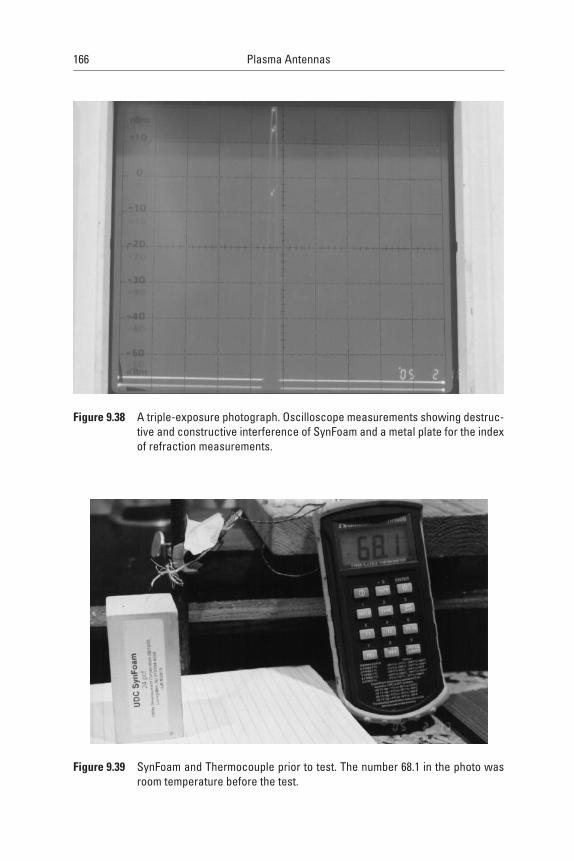
166 PlasmaAntennas
Figure 9.38 Atriple-exposurephotograph.Oscilloscopemeasurementsshowingdestruc-tiveandconstructiveinterferenceofSynFoamandametalplatefortheindexofrefractionmeasurements.
Figure 9.39 SynFoamandThermocouplepriortotest.Thenumber68.1inthephotowasroomtemperaturebeforethetest.

Experimental Work 167
Figure 9.40 SynFoam and Thermocouple after test indicating insignificant damage at1,200°Fin30-secondintervals.Thenumber498inthephotoisthetemperatureaftersignificantcooling.
Figure 9.41 SynFoam after test indicating insignificant damage at 1,200°F in 30-secondintervals.
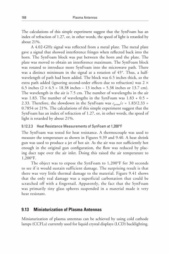
168 PlasmaAntennas
The calculations of this simple experiment suggest that the SynFoam has an index of refraction of 1.27, or, in other words, the speed of light is retarded by about 21%.
A 4.02-GHz signal was reflected from a metal plate. The metal plate gave a signal that showed interference fringes when reflected back into the horn. The SynFoam block was put between the horn and the plate. The plate was moved to obtain an interference maximum. The SynFoam block was rotated to introduce more SynFoam into the microwave path. There was a distinct minimum in the signal at a rotation of 45°. Thus, a half-wavelength of path had been added. The block was 6.5 inches thick, so the extra path added (ignoring second-order effects due to refraction) was 2 ´ 6.5 inches (2 ´ 6.5 = 18.38 inches – 13 inches = 5.38 inches or 13.7 cm). The wavelength in the air is 7.5 cm. The number of wavelengths in the air was 1.83. The number of wavelengths in the SynFoam was 1.83 + 0.5 = 2.33. Therefore, the slowdown in the SynFoam was cprime/c = 1.83/2.33 = 0.7854 or 21%. The calculations of this simple experiment suggest that the SynFoam has an index of refraction of 1.27, or, in other words, the speed of light is retarded by about 21%.
9.12.2.3 HeatResistanceMeasurementsofSynFoamat1,200°F
The SynFoam was tested for heat resistance. A thermocouple was used to measure the temperature as shown in Figures 9.39 and 9.40. A heat shrink gun was used to produce a jet of hot air. As the air was not sufficiently hot enough in the original gun configuration, the flow was reduced by plac-ing duct tape over the air inlet. Doing this raised the air temperature to 1,200°F.
The object was to expose the SynFoam to 1,200°F for 30 seconds to see if it would sustain sufficient damage. The surprising result is that there was very little thermal damage to the material. Figure 9.41 shows that the only real damage was a superficial carbonation that could be scratched off with a fingernail. Apparently, the fact that the SynFoam was primarily tiny glass spheres suspended in a material made it very heat resistant.
9.13 Miniaturization of Plasma Antennas
Miniaturization of plasma antennas can be achieved by using cold cathode lamps (CCFLs) currently used for liquid crystal displays (LCD) backlighting.

Experimental Work 169
These tubes come in many sizes and shapes and are available for most elec-tronics distributors (see [17]).
Ball-and-socket glass tubes inside plastic tubes can also be used for the miniaturization of plasma antennas. In this case, plastic tubes prevent air from contacting plasma and ball-and-socket joints allow for the bending and flexibility of plasma tubes (see [18]).
References
[1] Borg, G., et al., “Plasmas as Antennas: Theory, Experiment, and Applications,” Physics of Plasmas, Vol. 7, No. 5, May 2000, p. 2198.
[2] Borg, G. G., et al., “Application of Plasma Columns to Radiofrequency Antennas,” Appl. Phys. Lett., Vol. 74, No. 3272, 1999.
[3] Alexeff, I., and T. Anderson., “Experimental and Theoretical Results with Plasma Antennas,” IEEE Transactions on Plasma Science, Vol. 34, No. 2, April 2006.
[4] Alexeff, I., and T. Anderson, “Recent Results of Plasma Antennas,” Physics of Plasmas, Vol. 15, 2008, p. 057104.
[5] Anderson, T., and I. Alexeff, “Plasma Frequency Selective Surfaces,” IEEE Transactions on Plasma Science, Vol. 35, No. 2, April 2007, p. 407.
[6] Anderson, T., and I. Alexeff, “Reconfigurable Electromagnetic Waveguide,” U.S. Pat-ent No. 6,624,719, issued September 23, 2003.
[7] Anderson, T., and I. Alexeff, “Reconfigurable Electromagnetic Plasma Waveguide Used as a Phase Shifter and a Horn Antenna,” U.S. Patent No. 6,812,895, issued November 2, 2004.
[8] Anderson, T., and I. Alexeff, “Reconfigurable Scanner and RFID,” Application Serial Number 11/879,725, Filed 7/18/2007.
[9] Anderson, T., “Configurable Arrays for Steerable Antennas and Wireless Network Incorporating the Steerable Antennas,” U.S. Patent No. 7,342,549, issued March 11, 2008.
[10] Alexeff, I., “Pulsed Plasma Element,” U.S. patent 7,274,333, issued September 25, 2007.
[11] Anderson, T., “Tunable Plasma Frequency Devices,” U.S. Patent No. 7,292,191, is-sued November 6, 2007.
[12] Anderson, T., “Tunable Plasma Frequency Devices,” U.S. Patent No. 7,453,403, issued November 18, 2008.
[13] http://en.wikipedia.org/wiki/Lexan.

170 PlasmaAntennas
[14] http://www.ehow.com/facts_5612189_lexan-glass_.html.
[15] http://www.corninggorillaglass.com/.
[16] http://www.udccorp.com/products/SynFoamsyntacticfoam.html.
[17] http://www.jkllamps.com/files/BF20125-28B.pdf.
[18] http://en.wikipedia.org/wiki/Ground_glass_joint.

171
10Directional and Electronically Steerable Plasma Antenna Systems by Reconfigurable Multipole Expansions of Plasma Antennas
10.1 Introduction
The following multipole designs of plasma antennas are a result of perfectly zero mutual inductance for extinguished plasma antenna. PIN diodes can substantially reduce mutual impedance in similar metal antenna designs, but not as perfectly as extinguished plasma antennas can. The reader should re-view multipole expansions in Jackson [1], Feynman [2], and Pierce [3].
10.2 Multipole Plasma Antenna Designs and Far Fields
Steerable, directional, smart plasma antennas [private communication with I. Alexeff, 2007] can be made from a cluster of plasma antennas (Figure 10.1) when properly designed and programmed. In the far field such a configuration

172 PlasmaAntennas
can be a multipole expansion of transmitting and receiving plasma antennas when two or more plasma antennas are on and the rest are turned off (plasma gone).
To give the reader a better understanding of how the configuration of plasma tubes can have engineering form, the schematic in Figure 10.2 shows how the plasma antennas are housed in a rigid and hardened foam called SynFoam. SynFoam has an index of refraction close to 1 and is essentially transparent to electromagnetic waves.
The resulting electric far field from the two plasma antennas that are on and oscillating out of phase while the rest of the plasma antennas are off (as shown in Figure 10.3) is:
Figure 10.1 Topviewofaplasmaantennasurroundedbyaringofplasmaantennas.
Figure 10.2 TheplasmaantennaconfigurationofFigure10.1housedinSynFoam.

DirectionalandElectronicallySteerablePlasmaAntennaSystems 173
= − − +0 0cos ( cos ) cos ( cos )
2 2L L
E E k x E k xθ θ
(10.1)
where the angle q is given in Figure 10.4.Assume that the wavelength is large compared to the plasma antenna
system of diameter L so that:
<1
2kL
(10.2)
The resulting electric field is:
= 0(sin ) cosE E kx kL θ (10.3)
The electric field shows that this is a two-lobe radiation pattern but di-rectional, and the two lobes of the plasma antenna are oscillating out of phase.
Figure 10.3 A multipole plasma antenna configuration with two outside plasma antennasoscillatingoutofphasetoformadipole.Therestoftheplasmaantennasareoff.Thex-axisinallcasesconnectstheplasmaantennasthatareoff.Thex-axisandthereforetheantennalobescanberotatedorchangedasplasmaantennasareturnedonoroff.
Figure 10.4 Schematic todefinetheangleq.The lineconnectingtheplasmaantennasthatareonisdefinedasthex-axisforanyorientationofplasmaantennasthatareon.
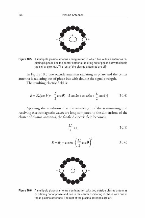
174 PlasmaAntennas
In Figure 10.5 two outside antennas radiating in phase and the center antenna is radiating out of phase but with double the signal strength.
The resulting electric field is:
= − − + +0[cos ( cos ) 2cos cos ( cos )]
2 2L L
E E k x kx k xθ θ
(10.4)
Applying the condition that the wavelength of the transmitting and receiving electromagnetic waves are long compared to the dimensions of the cluster of plasma antennas, the far-field electric field becomes:
<1
2kL
(10.5)
= −
2
0 cos cos2
kLE E kx θ
(10.6)
Figure 10.5 Amultipoleplasmaantennaconfigurationinwhichtwooutsideantennasra-diatinginphaseandthecenterantennaradiatingoutofphasebutwithdoublethesignalstrength.Therestoftheplasmaantennasareoff.
++−
Figure 10.6 Amultipoleplasmaantennaconfigurationwithtwooutsideplasmaantennasoscillatingoutofphaseandoneinthecenteroscillatinginphasewithoneoftheseplasmaantennas.Therestoftheplasmaantennasareoff.

DirectionalandElectronicallySteerablePlasmaAntennaSystems 175
This is a two-lobe plasma antenna with both lobes in phase.In Figure 10.6 the two outside plasma antennas are radiating out of
phase (a dipole). The center antenna is oscillating in phase with one of the antennas (in this case, the one on the right).
Using the long wavelength condition,
<1
2kL
(10.7)
the resulting far-field radiation E field from this plasma antenna configura-tion is:
0[1 cos ]sinE E kxθ= + (10.8)
This result represents a one-lobe directional radiation pattern.Multipole expansions of plasma antennas in which some are on and
the others are off yield directional antennas which can be steered by turning some of the plasma antennas on and off in a sequence. The key is that plasma antennas can be turned on or off, which is not possible with metal antennas. Smart plasma antennas can be designed when these multipole plasma antenna designs are computerized. Designs based on this concept are very applicable for mounting low-frequency, directional, and steerable smart antennas on vehicles, ships, and aircrafts where space is small. However, the applications are at all frequencies provided that the wavelength is long compared to the diameter of the cluster of plasma antennas.
References
[1] Jackson, J. D., ClassicalElectrodynamics, New York: John Wiley & Sons, 1962, 1975, 1998.
[2] Feynman, R., R. B. Leighton, and M. Sands, TheFeynmanLecturesonPhysics, Com-memorative Issue, Three-Volume Set, Reading, MA: Addison-Wesley, 1989.
[3] Pierce, A., Acoustics: An Introduction to Its Physical Principles and Applications, Section 4-4, Melville, MY: The American Physical Society through the American In-stitute for Physics, 1989.


177
11Satellite Plasma Antenna Concepts
11.1 Introduction
The reader should review satellite and reflector antennas in Kraus and Mar-hefka [1] and Balanis [2]. Plasma antennas have much less thermal noise (see Chapter 12) than metal antennas at satellite frequencies. Plasma antennas with plasma feeds (plasma waveguides and coaxial cables have been built) and low noise receivers can have higher data rates than corresponding metal antennas at satellite frequencies.
11.2 Data Rates
This section concerns data rates for comparison of plasma antennas with cor-responding metal antennas [3]. Keep in mind that what is important is the thermal noise of the entire antenna system and not just the antenna. Often-times the antenna is not the most important contributor of thermal noise in an antenna system. Satellite antennas that point to space interact with an equivalent thermal noise temperature of space and/or the sky of 5K. Never-theless, it is instructive to compare the data rates based on the thermal noise differences of a plasma antenna and a corresponding metal antenna [private communication with I. Alexeff].

178 PlasmaAntennas
Since noise is a random number, it accumulates as the square root of the integration time. For example, reducing the noise by a factor of 2 should up the data input rate by a factor of 4. Accumulated noise = random noise * square root of time. Our signal is coherent, and increases linearly with time. Accumulated signal = signal input * time. Thus, by keeping the accumulated signal to the accumulated noise constant so we can see our signal over the noise, and reducing the random noise by a factor of 2, our integrating time is reduced (because of the square root) by a factor of 4.
AS º Accumulated signal;
AN º Accumulated noise;
SI º Signal input;
RN º Random noise;
RNp º Random noise for plasma antenna;
RNm º Random noise for metal antenna;
t º integration time;
DRm º Data rate of metal antenna;
DRp º Data rate of plasma antenna.
The accumulated signal is given as the product of the signal input and integration time.
( )=AS SI t (11.1)
The accumulated noise is given as the product of the random noise and the square root of the integration time.
( )=AN RN t (11.2)
The ratio of the accumulated signal to the accumulated noise is:
= =AS SI t SI
tAN RN RNt
(11.3)
The random noise of the plasma antenna is reduced by a factor of 1/n compared to the random noise of a metal antenna
= m
pRN
RNn
(11.4)

Satellite Plasma Antenna Concepts 179
Substituting the random noise of the plasma antenna in terms of the random noise of the metal antenna and using expressions for the plasma and metal integration times yields:
2
/ mp p m
mm
AS SI SI SIt n t t
AN RN n RN RN= = =
(11.5)
=2p mn t t (11.6)
The data rates of the plasma antenna are now given in terms of the data rates of the metal antennas.
2 21/ ( 1/ )p p m mDR t n t n DR≡ = =
(11.7)
or
= 2p mDR n DM (11.8)
where n is the factor in which random noise is increased by using a metal antenna instead of a plasma antenna. As shown in Chapter 12, n >>1 for a fluorescent tube above 1.27 GHz, the thermal noise is less than in metal.
Focused and/or steered microwaves
Figure 11.1 Steering and focusing when the plasma density is above cutoff (reflectivemode).IncidentRFwavesontherightimpingeonplasmatubeswithdifferentdensities,butwiththeplasmadensitiesabovecutoff(reflectivemode).Focus-ingorsteeringcanbeachieveddependingonhowtheplasmadensitiesarevariedfromtubetotube.

180 PlasmaAntennas
Receiving or transmitting plasma orMetal horn antenna carrying signal toTV, and so forth.
Figure 11.2 Steering and focusing in two dimensions when the plasma frequency orplasmadensityisabovecutoff(reflectivemode).Basicplasmasatellite(otherfrequenciesapply)reflectorantennadesignwithtwobanksofperpendicularplasmatubesforsteeringand/offocusingintwodimensions.Thissystemcanapply to both a moving surface or a static surface and steer and/or focussatellitesignalsbyvaryingtheplasmadensityamongtheplasmatubeswithcomputercontrolsinspaceand/ortime.Thefirstbankoftubesontherighthasaplasmafrequencyorplasmadensitybelowcutoffandsteersandfo-cusesbyrefraction.Thesecondsetoftubesontherightsteersandfocusesbyreflectionandhasaplasmafrequencyorplasmadensityabovecutoff.
11.3 Satellite Plasma Antenna Concepts and Designs
An arrangement of plasma antennas can be flat and effectively parabolic. An arrangement of plasma antennas can electronically focus and steer RF signals without phased arrays [private communication with I. Alexeff]. Applications can be for both static (e.g., DIRECTV) and dish antennas attached to ve-hicles, ships, or aircraft.

Satellite Plasma Antenna Concepts 181
Figure 11.3 Steeringandfocusingintwodimensionswithbanksoftubesdisplacedwhentheplasmafrequencyorplasmadensityisabovecutoff(reflectivemode).OntheleftabandoftubescontainingplasmareflectsEMwavesandsteersandfocusesthebeaminonedirection.Ontherightaperpendicularbankoftubescontainingplasmareflects,steers,andfocusestheEMwavesintheperpen-diculardirection.AhornantennainthelowerrighttransmitsorreceivestheEMwaves.Thebanksoftubescontainingplasmacanbeflushwithasurfaceorsupportedinotherways.
Figures 11.1, 11.2, and 11.3 are schematics of RF wave beam steer-ing when the plasma densities or plasma frequencies of the plasma in the tubes are above cutoff. This is the reflective mode. Figures 11.4 and 11.5 are schematics of RF wave beam steering when the plasma densities or plasma frequencies are below cutoff. This is the refractive mode.
A plasma layer can reflect microwaves if the incident electromagnetic wave frequency is less than the plasma frequency [3]. A plane surface of plasma can steer and focus a microwave beam on a time scale of milliseconds. Cutoff is defined as the displacement current and the electron current cancelation

182 PlasmaAntennas
when electromagnetic waves impinge on a plasma surface. The electromag-netic waves are cut off from penetrating the plasma. The basic observation is that a layer of plasma beyond microwave cutoff reflects microwaves with a phase shift that depends on plasma density.
Exactly at cutoff, the displacement current and the electron current cancel. Therefore, there is an antinode at the plasma surface, and the electric field reflects in phase. As the plasma frequency or plasma density increases from cutoff, the reflected field increasingly reflects out of phase.
Hence, the reflected electromagnetic wave is phase-shifted depending on the plasma frequency or plasma density. This is similar to the effects of phased array antennas with electronic steering except that the phase shift-ing and hence steering and focusing come from varying the density of the plasma from one tube to the next and phase shifters used in phased array technology are not involved.
Steering and Focusing when the PlasmaFrequency or Plasma Density is Below Cutoff
Refractive Mode
Figure 11.4 Steeringandfocusingwhentheplasmafrequencyorplasmadensityisbelowcutoffrefractivemode.IncidentRFwavesontheleftimpingeonplasmatubeswith different densities but with the plasma frequencies or plasma frequen-ciesorplasmadensitiesbelowcutoff.Focusingorsteeringcanbeachieveddependingonhowtheplasmafrequenciesorplasmadensitiesarevariedfromtubetotube.

Satellite Plasma Antenna Concepts 183
Plasma physics allows us to use a layer of plasma tubes to reflect micro-waves [3]. By varying the plasma density in each tube, the phase of the reflected signal from each tube can be altered. The reflected signal can be steered and focused in analogy to what occurs in a phased array antenna. The steering and focusing of the mirror can occur on a time scale of milliseconds.
Plasma satellite (works at other operating frequencies) antenna is mounted between the received or transmitted antennasignals in which thetwo banks of tubeswith plasma withvariable plasmafrequency or densityfrom one tube to the next to steer andfocus the antennabeam.
Receiving or transmitting plasma or metal horn antenna carrying signal to TV, and so forth.This system eliminates the parabolic dish.
Figure 11.5 Steeringandfocusingintwodimensionswhentheplasmafrequencyorplasmadensityisbelowcutoff(refractivemode).Basicplasmasatellite(worksatotherfrequencies)antennadesignwithtwobanksofperpendicularplasmatubesforsteeringand/orfocusingintwodimensionswithplasmafrequenciesorplasmadensitiesbelowcutoff.Thisisintherefractivemode,notthereflectivemode.Thissystemcanapplytobothamovingsurfaceorastaticsurfaceandsteerand/orfocussatellitesignalsbyvarying theplasmadensityamong theplasma tubeswithcomputercontrolinspaceand/ortime.
184 PlasmaAntennas
Steering and focusing can also be achieved when the plasma density is below cutoff (see Figure 11.4). The steering and focusing of impinging elec-tromagnetic waves by plasma below cutoff are a consequence of the plasma lens effect. See Chen [4] and Linardakis et al. [5].
An effective Snell’s law causes refraction of electromagnetic waves passing through a plasma of variable density (plasma density varying from container to container containing plasma). The speed of electromagnetic waves in a plasma is a function of plasma frequency or plasma density.
Feed horns and receivers can be put behind satellite plasma antennas operating in the refractive mode. This eliminates the problem of the blind spot and feed losses caused by the feed horn and receiver in front of a metal satellite antenna. This phenomenon is also known as a convergent or convex plasma lens. A convergent plasma lens can focus electromagnetic waves to decrease beamwidths and increase directivity and antenna range. A divergent plasma lens can also be created. Both convergent and divergent plasma lenses lead to reconfigurable beamwidths.
An electronically steerable and focusing plasma reflector antenna can be made by having plasma densities in the tubes above cutoff but with the plasma densities varying from tube to tube. An electronically steerable and focusing bank of plasma tubes can be made by having plasma densities in the tubes below cutoff but with the plasma frequencies or plasma densities varying from tube to tube. Electronic steering and focusing in either of these cases can be made in two dimensions by having two perpendicular banks of tubes. This can also steer and focus horizontal, vertical, circular, and ellipti-cally polarized signals.
With plasma electronic steering and focusing, parabolic reflector anten-nas are not needed. This is in many ways a superior alternative to electronic steering with phased arrays.
More research, both experimentally and theoretically, is needed on the effects of plasma density fluctuations. On various prototypes to date, for ex-ample, on the plasma reflector antenna at 3 GHz, density fluctuations have been insignificant or nonexistent and have had no effect on performance.
References
[1] Kraus, J., and R. Marhefka, Antennas for All Applications, 3rd ed., New York: McGraw-Hill, 2002, Section 21-14.
[2] Balanis, C., Antenna Theory, 2nd ed., New York: John Wiley & Sons, 1997, Chapter 15.

Satellite Plasma Antenna Concepts 185
[3] Krall, N., and A. Trivelpiece, Principles of Plasma Physics, New York: McGraw-Hill, 1973, Sections 4.5.1 and 4.5.2.
[4] Chen, F., Introduction to Plasma Physics and Controlled Fusion, Volume 1, 2nd ed., New York: Plenum Press, 1984, p. 119.
[5] Linardakis, P., G. Borg, and N. Martin, “Plasma-Based Lens for Microwave Beam Steering,” Electronics Letters, Vol. 42, No. 8, April 2006, pp. 444–446.

187
12Plasma Antenna Thermal Noise
12.1 Introduction
G. G. Borg et al. [1] discussed noise by comparing the noise spectra of recep-tion of three antennas. Two antennas are plasma antennas and one antenna is a metal antenna. The frequency of reception was a 21-MHz, 1-mW source. The first antenna was a plasma antenna of length 1.2m driven by 240-V, 50-Hz AC applied between electrodes. The second antenna was 2.2m in length and driven by surface wave excitation of 140 MHz. The third antenna was a metal antenna, but no length was specified. Borg et al. [1] concluded that the noise performances of the surface wave driven plasma antenna and the metal antenna were the same, but the 50-Hz AC driven plasma antenna had noise floors 10 to 30 dB higher across the band. It is shown below that the thermal noise in a plasma antenna as a fluorescent tube is lower than a corre-sponding metal antenna above 1.27 GHz, but higher below 1.27 GHz. This crossover point can be reduced by lowering the pressure in the fluorescent tube. However, Borg et al. concluded that low-frequency driven AC or DC excited plasma tubes would have limited applications in communications. However, Anderson and Alexeff built such plasma antennas with fluorescent tubes, which receive FM and AM signals well. Borg et al. also concluded that plasma antennas operating at low-frequency AC or at DC would have to be operated in the afterglow for reception. It is not clear why there would be afterglow if there is no pulsing. See Chapter 4 and [2]. Borg et al. [1] also concluded that plasma antennas operating at low-frequency AC or at DC

188 PlasmaAntennas
would have to be operated in the afterglow for reception. It is not clear why there would be afterglow if there is no pulsing. Again, Anderson and Alexeff built low-frequency AC and DC plasma antennas that receive FM and AM signals well.
12.2 Modified Nyquist Theorem and Thermal Noise
This material is an expansion of the work in [3] for the standard Nyquist’s theorem in which the well-known result is H = 4RKT, where H is the noise spectrum as volts squared per hertz (not watts), R is the resistance of the ob-ject in ohms (not ohms per unit length), K is Boltzmann’s constant in Joules per degree K, and T is the temperature in degrees K.
The equation is a low-frequency approximation, but this approxima-tion is correct, since in metals the collision frequency is a terahertz.
The correction term found by Anderson [4–6] is derived here.
= +
2
2
14
(2 )1
cc
H RKTπυν
(12.1)
where u is the frequency of the transmitter in hertz and ncc is the electron-gas atom collision frequency in hertz.
The correlation function for the noise voltage V(t) is:
( )ττ τ τ τ= = + = −∑ ∑ ∑ 2
0( ) ( ) ( ) ( )i i i i
i i i
R R V t V t V
(12.2)
assuming that the stochastic nature of plasma thermal noise is Poisson dis-tributed. Using the Wiener-Khintchine theorem [3, pp. 585–587; 7], we obtain the power spectral density of plasma noise.
¥
¥
= =
-
ò
åò
0
2
0
( ) 4 ( )cos(2 )
4 exp( )cos(2 )i cci
H f R f d
V f d
t p t t
ν t p t l
(12.3)
PlasmaAntennaThermalNoise 189
where R is the resistance in ohms and e is the charge of the electron, and the collision frequency is:
ν τ= 1cc
o (12.4)
The voltage fluctuation V is related to the electron velocity fluctuation u as follows:
=i i
eV R u
l (12.5)
ρ ρ= =l A
R RA l
where R is the resistance in Ohms and e is the charge of the electron. A is the cross-sectional area of a plasma section of constant radius, l is the length of the plasma section, and r is the resistivity in ohms-meters. Hence, the ther-mal noise power spectral density becomes:
τ ωτ ττ-æ öæ ö= ç ÷ ç ÷è ø è øò
22
0
Re( ) 4 exp cos( )H f n u d
l
τω τ
νων
æ ö= ç ÷è ø +
æ ö= ç ÷è ø æ ö+ ç ÷è ø
22 0
2 20
22
2
Re4
1
Re 1/4
1
cc
cc
n ul
n ul
(12.6)
where
=∑
22
n
ii
u n u (12.7)
where ncc is the collision frequency and n is the number of plasma particles.Using the relationship from kinetic theory:
=21 1
2 2m u kT
(12.8)

190 PlasmaAntennas
and the conductivity relationship:
= =
2 1
cc
n'em
σ ν ρ
(12.9)
where the plasma density is:
′ = =n nn V Al (12.10)
Substituting these quantities into the power spectral density for the plasma noise yields:
( )( )
τ νω τ ω
n
= = = + +
222 20
2 2 20
Re Re 1/( ) 4 4
1 1
cc
cc
H f n u n ul l
= = = + + +
22 2
2 2 2 2 2
2 2 2
Re 4 4 4
1 1 1cccc cc
cc cc cc
le nn kRT kRT e n kRTA
Almvl m l mv
ρρ
ν ω ω ων ν ν
′ = = + + +
2
2 2 2
2 2 2
4 ) 4 4(1)
1 1 1cc
cc cc cc
e n kRT kRT kRTm
ρ ρσ ν ω ω ω
ν ν ν (12.11)
( )ων
=+
2
2
4
1cc
RH f kT
(12.12)
For a metal antenna, ncc >> w.
=( ) 4metalH f kTR (12.13)

PlasmaAntennaThermalNoise 191
To compare the noise [private communication with Igor Alexeff, 2008] in a given spectral region, R and ncc for metals and for plasmas must be obtained. Considering the operation at 10 GHz (3-cm wavelength), in metals nc from [2] is 1 THz.
For the resistance, assume a rod 1 cm square in a cross-section and 3 cm long. The resistance of copper is 1.692exp(–6) [8], so the metal antenna would be 5.076exp(–6) ohms if skin depth were to be neglected.
Skin depth is given by
122
σµω (12.14)
where s is the conductivity, m is the permittivity, and w is the angular frequency of the microwaves (radians per second or 2pu in hertz).
The skin depth is 2exp(–5) cm. Hence, the resistivity corresponds to a copper sheet is 3 cm long, 4 cm wide, and 2exp(–5) cm thick. This corresponds to a resistance of 0.063 ohm. The temperature of the copper is 300K.
For the plasma, the collision frequency is computed as follows. In [9], the pressure in a fluorescent tube is a maximum of 2 mmHg. The electron-gas atom scattering cross-section, corresponding to an electron tempera-ture of 1 electron-volt, is deep in the Ramsauer minimum. The mean free path is about 1 cm at a pressure of 1 mmHg. This gives a scattering cross- section of 2.8exp(–17) cm squared (it is at the Ramsauer minimum), at a pressure of 1 mmHg.
The electron velocity corresponds to 1 electron-volt. The thermal ve-
locity is = KTv
m where v is the velocity, K is Boltzmann’s constant,T is the
electron temperature, and m is the electron mass. Inserting the proper values gives an electron thermal velocity of 4.2exp(7) cm per second. Using the atom density at s mmHg to be 7.02exp(17) per cc, the collision frequency is computed to be 82 MHz. Actually, if the tube is about 1 cm in diameter, the collision frequency at the wall exceeds this.
In regards to the resistance of the tube, Cobine [8] gave the voltage drop for a 9-inch tube to be 45 and for a 48-inch tube to be 108. Subtract-ing these to get rid of the cathode drop and to find the voltage drop on the positive column, we get 1.62 volts per inch, or 0.638 volt per cm. The current ranged from 0.15 to 0.42 ampere. Since the tube has essentially a voltage drop independent of the current, we use the 0.42-ampere value. This yields a resistance of 1.52 ohms per cm. For a 3-cm-long column of plasma, we have 4.56 ohms.

192 PlasmaAntennas
Computing the noise figure in volts squared per hertz, the metal gives us 1.04exp(–21).
For the plasma antenna at 10 GHz, we obtain 4.29exp(–24).Thus, in this frequency range, the noise in the plasma antenna is much
less than the metal antenna. Of course, at low enough frequencies, the in-equality is reversed, but we can address that by reducing the gas pressure in custom-made plasma tubes.
Note that we used the upper limit for gas pressure in this report on the plasma tube. In the patent application, pressures 2,000 times lower have been used [10]. Using the lowest pressure would reduce the plasma noise by about a factor of 2,000.
Keep in mind that this analysis has been and is for a fluorescent lamp. Plasma antennas have been made out of fluorescent lamps because they are inex-pensive and the use of fluorescent lamps shows that people can do research and development and build prototypes of the plasma antenna technology cheaply.
When plasma antennas are ruggedized with custom-made plasma tubes, the gas pressure inside the plasma tubes can be made much less than in a fluorescent bulb and can lower the frequency at which the plasma antenna thermal noise is equal to the metal antenna thermal noise.
Using the highest gas pressure in a fluorescent tube of 2 millimeters, the frequency at which the plasma antenna and the metal antenna have the same thermal noise is 1.27 GHz. Using the lowest gas pressure of a fluorescent tube of 1 micron, this crossover frequency at which the plasma antenna thermal noise and the metal antenna thermal noise are equal is much lower. Above the crossover frequency of the thermal noise of the plasma antenna and the metal antenna, the plasma antenna thermal noise drops rapidly.
As stated earlier, custom-made plasma tubes can be made such that pressure is much lower than in a fluorescent lamp. This would give a number in which the thermal noise of the plasma antenna and the metal antennas are equal much lower than a 1.27-GHz antenna frequency.
Again, fluorescent tubes have been used often to make plasma antennas be-cause this has been an inexpensive way to do plasma antenna research and devel-opment. Custom-made plasma tubes are being planned to have a rugged design and to have lower noise than metal antennas over a very wide frequency range. A patent has been filed on low thermal noise designs of plasma antennas [11].

PlasmaAntennaThermalNoise 193
References
[1] Borg, G. G., et al., “Plasmas as Antennas: Theory, Experiment, and Applications,” PhysicsofPlasmas, Vol. 7, No. 5, May 2000, p. 2198.
[2] www.ionizedgasantennas.com.
[3] Reif, F., Fundamentals of Statistical and Thermal Physics, New York: McGraw-Hill, 1965, Sections 5.15 and 5.16, pp. 585–589.
[4] Anderson, T., “Electromagnetic Noise from Frequency Driven and Transient Plas-mas,” IEEE International Symposium on Electromagnetic Compatibility, SymposiumRecord, Vol. 1, Minneapolis, MN, August 19–23, 2002.
[5] http://www.mrc.uidaho.edu/~atkinson/Huygens/PlasmaSheath/01032529.pdf.
[6] Anderson, T., “Control of Electromagnetic Interference from Arc and Electron Beam Welding by Controlling the Physical Parameters in Arc or Electron Beam: Theoretical Model,” 2000IEEESymposiumRecord, Vol. 2, 2000, pp. 695–698.
[7] Pierce, A. D., Acoustics: An Introduction to Its Physical Principles and Applications, Section 2-10, Melville, NY: American Physical Society/American Institute for Physics, 1989. pp. 85–88.
[8] CRCHandbookChemistryandPhysics, 85th Edition, 2004.
[9] Cobine, J. D., Gaseous Conductors Theory and Engineering Applications, New York: McGraw-Hill, 1941.
[10] U.S. Patent, “Plasma Tube Pressures,” No. 1,790,153, issued January 27, 1931.
[11] Anderson, T., and I. Alexeff, “High SNR Plasma Antenna,” Application Serial Number 12/324,876, November 27, 2008.


195
About the Author
Dr. Theodore R. Anderson (sometimes referred to as Dr. Ted Anderson) is a foremost authority and pioneer on plasma antennas. Dr. Anderson has over 20 issued patents on plasma antennas, plasma frequency selective sur-faces, and plasma waveguides. He has published several peer reviewed jour-nal articles on plasma antennas, and has presented at many conferences with symposium papers on plasma antennas. He founded Haleakala Research and Development, Inc. in 2002, which became a company focused on the plasma antenna technology. His contact information is tedanderson@haleakala- research.com; [email protected]; and 518–409–1010.
Dr. Anderson received his Ph.D. in physics from New York University in 1986, an M.S. in physics from New York University in 1979, and an M.S. in applied science from New York University in 1983. He also studied foun-dations of quantum mechanics and mathematical scattering theory under the renowned physicist J. M. Jauch at the Department de Physique Theorique at the University in Geneva, Geneva, Switzerland.
He has published in the areas of plasma antennas, plasma physics, electrodynamics, fluid dynamics, acoustics, hydroacoustics, atomic physics, foundations of quantum mechanics, and mathematical scattering theory. He considers himself a generalist with wide interests in physics and engineering.
His corporate experience has been in nuclear engineering at Gibbs and Hill Inc., fluid dynamics and acoustics at Electric Boat, General Dynamics; antennas, fluid dynamics, hydroacoustics, and acoustics at the Naval Under-sea Warfare Center; and submarine nuclear engineering at Knolls Atomic Power Laboratory.
Dr. Anderson has taught a variety of subjects in several universities including mechanical, ocean engineering, marine sciences, and astronomy at the University of Connecticut, Avery Point; electrical, mechanical, and nuclear engineering at Rensselaer Polytechnic Institute at both the Troy and Hartford campuses; mechanical engineering at Union College; electrical
Art_Anderson_ATA.indd 195 Manila Typesetting Company 06/24/2011 01:20PM

196 PlasmaAntennas
engineering, mechanical engineering, and business statistics (in the business school) at the University of New Haven; mechanical, aeronautical, and man-agement engineering at the University of Bridgeport; electrical engineering at Cooper Union School of Engineering; and physics and astronomy at Hunter College.
Dr. Anderson is a theatre and opera enthusiast and is working on a play. He has been a competitive power lifter and has set several records in New England and has won more than 40 trophies in this sport.
Please see the Web site: www.ionizedgasantennas.com for more infor-mation.
Art_Anderson_ATA.indd 196 Manila Typesetting Company 06/24/2011 01:20PM

Index
Accumulated noise, 178Adaptive array smart antennas, 80Adaptive directionality
advantages, 110illustrated, 110signal-to-noise ratio levels, 111smart plasma antennas, 110–11
See also Smart plasma antennasAgile mirror, 2Antenna lobes, 109
Ball-and-socket glass tubes, 169Ballasts, 39Barrier penetration, 28–29
electric field, 27plot, 29
BASIC Stamp 2, 84, 85BASIC Stamp module, 84Battery powered plasma antenna, 42–43Beam/pattern tracking algorithm, 106Bessel functions
divergence, 121field inside cylinder, 119zeroth-order, 73
Bessel’s equation, 25Bohm-Gross dispersion, 18Building plasma antennas, 37–44
design I, 38–41design II, 41–43design III, 44
electrical safety warning, 37introduction to, 37materials, 42–43
Cartesian coordinates, 62Cell towers
angle of service, 111benefits of plasma use with, 111–12smart plasma antennas on, 111–12
Coaxial plasma closing switch, 130, 131Code division multiple access (CDMA), 108Cold cathode lamps (CCFLs), 168Collision frequency, 191Compact fluorescent lamps (CFL), 157Corning Gorilla Glass, 162Cosite interference
occurrence of, 3reduction, 49
COTS tubes, 6Current density
definition of, 18equation solution, 76Fourier expansion of, 22
Custom-made plasma tubes, 192Cylindrical plasma
defined, 101Fabry-Perot resonators, 98–103plasma decay, 102plasma frequency, 102resonance, 101–2
197

Cylindrical plasma (continued)switching speeds, 103
Cylindrical symmetry, 119
Data rates, 177–79Dielectric constant, 32Dielectric permittivity, 26Dielectric-vacuum interface, 17Discharge columns, 17Driving field, 75
Elastic differential scattering cross section, 24Electrical safety warning, 37Electric fields
aligned with cylinder axis, 120barrier penetration, 26continuity at cylinder boundary, 119expansion of, 120–21linear antenna, 73polarization, 116scattered, 117tangential component of, 121wave equation for, 118
Electromagnetic boundary value problem,63–64
Electronic warfare protection experiments,130
Electronscontinuity equation, 31ionized, 118motion, 31perturbed density, 31temperature, 191velocity fluctuation, 35, 189
Embedded plasma antennasin sandstone slurry, 163in SynFoam, 163–68
Epoxy slurries, 162Excitation frequency, 3Expansion coefficients, 119Experimental work, 129–68
high-power plasma antennas, 148–54introduction to, 129miniaturization, 168–169plasma antenna, 129–37plasma antenna nesting, 146–48plasma density measurements, 154–62plasma frequency measurements, 154–62plasma FSS, 141–43plasma waveguides, 140–41
pulsing technique, 144ruggedization, 162–68
Fabry-Perot cavitiesdefined, 94interior surfaces, 94mathematical model for, 95–96
Fabry-Perot effects, 94, 102Fabry-Perot-Etalon effects, 93, 95Fabry-Perot resonators
advanced theory, 103cylindrical plasma, 98–103definitive tests, 103experimental setup, 100oscilloscope, 101reflection in, 95slab plasma, 96–97for smart plasma antenna, 93–103
Far-field radiation patterns15-cylinder plasma antenna, 61
for geometry solutions, 59plasma windows, 66–67PWA, 57
Finite element solution techniques, 25–30Fluid model, 13Fluorescent lamps, 38, 39Frequency selective surfaces (FSS)
layers, 113plasma, 113–27
Gauss’s law, 32Glow discharge plasmas, 15Gorilla glass tubes, 7GPS-aided positioning, 103–4GPS-free positioning, 104–6
beam/pattern tracking algorithm, 106illustrated, 106localization protocol, 105plasma tubes, 105research, 105
Hankel functionsaddition theorem, 64–65, 76partial wave expansion and, 64–65
Heat resistance, SynFoam, 168High-frequency plasma antennas, 3–4High-power plasma antennas, 148–54
cable system used for, 149conclusions on, 152–54experimental confirmation, 150–51
198 Plasma Antennas

introduction to, 148operation of, 152–54problem, 148pulsed power apparatus schematic, 149schematic, 152solution, 150voltage amplification on impedancemismatch, 150
Homogeneous wave equation, 71
Index of refraction, SynFoam, 165–68, 172Infrared signatures, 6Inhomogeneous wave equation, 70Interference
cosite, reduction, 49plasma antennas, 3–4windowing and, 56
Lexan glass, 7, 162Liquid crystal displays (LCDs), 168Localization protocol, 105Lucent BLAST system, 107–8
Magnetic ballast, 39Magnetic fields, 120Magnetohydrodynamic (MHD) equations,
14Man-made plasmas, 14–15Materials, for battery powered plasma
antennas, 42–43Matrix problem, 65–66Maxwell’s equations, 119–20Mechanical reconfigurability experiments,
130Mechanical robustness, 162–68Microcontroller, for smart plasma antenna,
84–86Microwave interferometers
balanced legs, 156instantaneous phase shift measurement,
156Ku-band waveguide, 155plasma density/frequency measurementswith, 154–62reflection experiments, 158, 159–62
Miniaturization, of plasma antennas,168–169
Modified Nyquist theorem, 188–92Momentum equation, 31
Multihop meshed wireless distributionnetwork architecture, 106–8
defined, 107illustrated, 107Lucent BLAST system, 107–8signal to interference and noise ratio
(SINR), 108Multipath-induced positioning error, 104Multiple-input-multiple output (MIMO)
processing, 108Multipole plasma antenna designs, 171–75
far fields and, 171–75housed in SynFoam, 172introduction to, 171key to, 175oscillating out/in phase, 174oscillating out of phase to form dipole,
173radiating in phase, 174ring, 172in steerable system, 171–75
Nested plasma antennasconcept, 48–49dipole inside helical, 46example of, 48experimental apparatus, 147experiments, 50–52, 146–48schematic conceptual design, 47testing, 47
Net radiated power, 31–33Neumann function, 73Newton’s equations of motion, 20Noise
accumulated, 178figure, computing, 191power spectral density, 188–89, 190random, 178–79thermal, 4–5, 34–36, 187–92
Nyquist theorem, 188
One-fluid model, 14Open plasma window indicator, 89, 90Organization, this book, 1–2
Partial wave expansion, 64–65Periodic Moment Method, 115–17Phase shift, 156Phenomenological damping, 20
Index 199

Plasma antenna arraysbandwidth, 47stacked, 48–49
Plasma antennasbuilding, 37–44characteristics of, 2cosite interference reduction with, 49COTS tubes as, 6embedded, 163–68experimental work, 129–37finite element solution techniques, 25–30with fluorescent and neon tubes, 6as FM antennas, 44high-frequency, 3–4high-power, 148–54infrared signature and, 6interference, 3–4miniaturization, 168nested, 46–49net radiated power, 31–33operating frequency, 3plasma fluid equations and, 18–21plasma physics for, 13–30Poynting vector, 22–24prototypes, 3RCS, 4reconfigurable impedance, 33–34reconfigurable multipole expansions of,
171–75reflector, 2ruggedization, 162–68satellite, 5, 177–84smart, 53–77, 79–112in SynFoam, 6–7testing, 39theory, 31–36thermal noise, 4–5, 34–36, 187–92windowing, 53–77
Plasma capacitive sleeve coupling, 39Plasma charge
definition of, 18local imbalance, 19
Plasma coaxial cables, 6Plasma cylinders
defined, 17incident signal, 21–22isolation of, 65in plasma waveguides, 140reflectivity of, 28
scattering off, 17–18touching, 61of unit radius, 26
Plasma density, 16cutoff, 182estimating, 154measurements with microwave
interferometer, 154–62phase-shifted electromagnetic waves and,
182by pulsed power technique, 144steering/focusing and, 179, 181, 182, 183
Plasma fluid equations, 18–21application of, 21charge densities from, 23plasma current from, 23
Plasma frequencyexcitation frequency versus, 3measurements, 154measurements with microwave
interferometer, 154–62of metal antenna, 3as natural frequency of plasma, 4proportional to density of unbounded
electrons, 4scaling function versus, 122selective surfaces, 6switchable reflector, 125as twice the operating frequency, 4
Plasma frequency selective surfaces, 113–27change in filtering, 113dipole array schematic, 123experimental setup, 143experimental work, 141–43laboratory, 114lab setup, 143method of calculation, 115–17Periodic Moment Method, 115–17in removing second/higher harmonics,
142results, 123–27scattering from partially conducting
cylinder, 117–23shielding, 114structure, 114switchable bandstop filter, 123switchable reflector, 124–27theoretical calculations and numerical
results, 114–23
200 Plasma Antennas

transmission and reflection characteristics,114
between transmitter and receiver, 141–43transparency, 113
Plasma physics, 13–30electromagnetic waves, 45–47mathematical models of, 13–14one-fluid model, 14of reflection and transmission, 15–17two-fluid model, 13
Plasma reflector antennascomparison tests, 131conclusions on, 140early, 131illustrated, 133, 134noise level, 137plasma configuration, 133plate spacing, 133radiation patterns, 136sidelobes, 136, 137tube spacing, 133–35
Plasmascurrent conduction, 45dense, generation at low average power
input, 90–93dielectric constant, 32electromagnetic waves, 26, 45–47electron motion, 31fixed degree ionization, 19glow discharge, 15man-made, 14–15power spectral density, 36wave phenomenon, 14
Plasma shields, 88–89Plasma transmitting folded dipole antennas,
132Plasma tubes
arrangement of, 68attenuation E-field parallel to, 92attenuation E-field perpendicular to, 92custom-made, 192cylindrical ring of, 101–2fluorescent lamps, 81in GPS-free positioning, 105ionization, 144parallel and perpendicular, 85plasma reflector antennas, 133–35plasma waveguides, 141polarization effect on, 88–90
pulse mode, 135pulsing techniques, 146to reflect microwaves, 183satellite plasma antennas, 181, 183in smart plasma antennas, 81source field interaction, 70spark-gap electrical schematic, 135SynFoam housing for, 164
Plasma waveguides, 6, 140–41defined, 130design illustration, 142illustrated, 141plasma tubes, 141types of, 140
Plasma window antenna (PWA)beam half-width versus wavelength, 62far-field radiation pattern, 57geometric construction, 59–63half beamwidth versus wavelength, 60radiated influx plot, 58seven cylinders, 58
Plasma windowsdissipation in, 67–77electromagnetic boundary value problem,
63–64far-field radiation pattern, 66–67fifteen touching cylinders, 60matrix problem, 65–66moving charges, 71open indicator, 89, 90opening/closing apertures, 68partial wave expansion, 64–65plasma radome made of, 54scattering fields solution, 66theoretical analysis, 57–77
See also WindowingPolarization
effect on plasma tubes, 88–90electric field, 116
Potentiometers, 151, 152Power pulsing, 90–93Poynting vector, 22–24
radial component, 67radiation intensity by computing, 67time-averaged, 24
Pulsed power apparatus, 149Pulsing techniques, 5
afterglow density, 145apparatus, 145
Index 201

Pulsing techniques (continued)experiments, 144–46plasma loss, 145plasma tubes, 146
Radiated powernet, 31–33total, 32
Radiation patternsfar-field, 57, 59for plasma antenna windowing device,
67–77plasma reflector antennas, 136PWA configuration, 59sixteen-lobe, 68windowing and, 56–57
RAKE receivers, 108Ramsauer-Townsend effects, 5Random noise, 178–79Reconfigurability
experiments, 130mechanical, 130
Reconfigurable bandwidth, 86Reconfigurable beamwidth, 108–9Reconfigurable impedance, 33–34Reconfigurable multipole expansions,
171–75Reflection coefficients, 15, 16Resonance effect, 100Ruggedization, 162–68
experiments, 130methods, 162sandstone slurry, 163SynFoam, 163–68thermal noise and, 192
Ruggedized smart plasma antenna prototype,91
Sandstone slurry, 163Satellite plasma antennas, 5, 177–84
arrangement of, 180concepts and designs, 180–83data rates, 177–79introduction to, 177plasma tubes, 181, 183steering and focusing, 180
See also Plasma antennasS-band modulator system, 156S-band waveguide reflection experiments,
159–62
negative polarity microwave detector, 158pressure, 159, 160, 161, 162
Scaling functioncalculation of, 28–30definition of, 28plasma frequency versus, 122plot, 29, 30in scattering analysis, 121for squared current, 118
Scatteringanalysis with scaling function, 121fields, 66, 75from partially conducting cylinder,
117–23Self-field, 73, 74Shielding experiments, 130Signal to interference and noise ratio (SINR),
108Skin depth, 191Slab plasma, Fabry-Perot resonators, 96–97Smart antennas, 79–80
adaptive array, 80defined, 79switched beam, 80uses, 79
Smart plasma antennasapplications in wireless technologies,
103–12block schematic, 84commercial prototype, 86commercial prototype illustration, 88computer, 83computer input interface, 82–83computer output interface, 83concept, 82design, 53–57early design and experimental work,
80–84early lab photo, 81Fabry-Perot resonator for, 93–103introduction to, 79laboratory setup, 82microcontroller for, 84–86with open plasma window indicator, 89polarization effect on plasma tubes, 88–90programmable antenna pattern, 106prototype, 80reconfigurable bandwidth, 86–87ruggedized prototype, 91
202 Plasma Antennas

scanning rate, 82video, 79windowing concept, 53–57
See also Plasma antennasSnell’s law, 184Source field, 77Spark gap techniques, 5–6, 137
circuit diagrams, 138electrical schematic, 135EMI noise suppression/elimination,
138–40experiments using, 138oscilloscope, 139, 140
Stacked plasma antenna arrays, 48–49Stealth experiments, 129Steerable plasma antenna systems, 171–75Switchable bandstop filter, 123Switchable reflector, 124–27
experimental results, 126illustrated, 125plasma frequency, 125theoretical/experimental plots exposed,
126Switched beam smart antennas, 80SynFoam, 6–7, 162
block rotation, 168defined, 163destructive/constructive interference, 166embedded plasma antennas, 163heat resistance measurement of, 168housing for plasma tubes, 164index of refraction, 172index of refraction measurement, 165–68RF radiation transparency, 165transmission and reflection experiments,
165
Thermal noise, 4–5, 34–36, 187–92
derivations on, 34introduction to, 187–88modified Nyquist theorem and, 188–92plasma versus metal antennas, 177–78power density spectrum, 35power spectral density, 189ruggedization and, 192
Transmission coefficients, 15Transmission/reception experiments, 129Two-fluid model, 13
Velocity-dependent damping force, 75Voltage fluctuation, 35, 189
Wave phenomenon, 14Wiener-Khintchine theorem, 35, 188Windowing, 53–77
advantages, 56beam forming schematic, 55beamwidth, 56concept, 53–57defined, 57device with plasma tubes, 85interference and, 56plasma antenna, top view, 55radiation patterns and, 56–57single-lobe plasma antenna, 54
Wireless technology applicationsadaptive directionality, 110–11cell tower setting, 111–12GPS-aided positioning, 103–4GPS-free positioning, 104–6introduction to, 103multihop meshed wireless distributionnetwork architecture, 106–8reconfigurable beamwidth and lobe
number, 108–9See also Smart plasma antennas
Index 203


专注于微波、射频、天线设计人才的培养 易迪拓培训 网址:http://www.edatop.com
射 频 和 天 线 设 计 培 训 课 程 推 荐
易迪拓培训(www.edatop.com)由数名来自于研发第一线的资深工程师发起成立,致力并专注于微
波、射频、天线设计研发人才的培养;我们于 2006 年整合合并微波 EDA 网(www.mweda.com),现
已发展成为国内最大的微波射频和天线设计人才培养基地,成功推出多套微波射频以及天线设计经典
培训课程和 ADS、HFSS 等专业软件使用培训课程,广受客户好评;并先后与人民邮电出版社、电子
工业出版社合作出版了多本专业图书,帮助数万名工程师提升了专业技术能力。客户遍布中兴通讯、
研通高频、埃威航电、国人通信等多家国内知名公司,以及台湾工业技术研究院、永业科技、全一电
子等多家台湾地区企业。
易迪拓培训课程列表:http://www.edatop.com/peixun/rfe/129.html
射频工程师养成培训课程套装
该套装精选了射频专业基础培训课程、射频仿真设计培训课程和射频电
路测量培训课程三个类别共 30 门视频培训课程和 3 本图书教材;旨在
引领学员全面学习一个射频工程师需要熟悉、理解和掌握的专业知识和
研发设计能力。通过套装的学习,能够让学员完全达到和胜任一个合格
的射频工程师的要求…
课程网址:http://www.edatop.com/peixun/rfe/110.html
ADS 学习培训课程套装
该套装是迄今国内最全面、最权威的 ADS 培训教程,共包含 10 门 ADS
学习培训课程。课程是由具有多年 ADS 使用经验的微波射频与通信系
统设计领域资深专家讲解,并多结合设计实例,由浅入深、详细而又
全面地讲解了 ADS 在微波射频电路设计、通信系统设计和电磁仿真设
计方面的内容。能让您在最短的时间内学会使用 ADS,迅速提升个人技
术能力,把 ADS 真正应用到实际研发工作中去,成为 ADS 设计专家...
课程网址: http://www.edatop.com/peixun/ads/13.html
HFSS 学习培训课程套装
该套课程套装包含了本站全部 HFSS 培训课程,是迄今国内最全面、最
专业的HFSS培训教程套装,可以帮助您从零开始,全面深入学习HFSS
的各项功能和在多个方面的工程应用。购买套装,更可超值赠送 3 个月
免费学习答疑,随时解答您学习过程中遇到的棘手问题,让您的 HFSS
学习更加轻松顺畅…
课程网址:http://www.edatop.com/peixun/hfss/11.html
`

专注于微波、射频、天线设计人才的培养 易迪拓培训 网址:http://www.edatop.com
CST 学习培训课程套装
该培训套装由易迪拓培训联合微波 EDA 网共同推出,是最全面、系统、
专业的 CST 微波工作室培训课程套装,所有课程都由经验丰富的专家授
课,视频教学,可以帮助您从零开始,全面系统地学习 CST 微波工作的
各项功能及其在微波射频、天线设计等领域的设计应用。且购买该套装,
还可超值赠送 3 个月免费学习答疑…
课程网址:http://www.edatop.com/peixun/cst/24.html
HFSS 天线设计培训课程套装
套装包含 6 门视频课程和 1 本图书,课程从基础讲起,内容由浅入深,
理论介绍和实际操作讲解相结合,全面系统的讲解了 HFSS 天线设计的
全过程。是国内最全面、最专业的 HFSS 天线设计课程,可以帮助您快
速学习掌握如何使用 HFSS 设计天线,让天线设计不再难…
课程网址:http://www.edatop.com/peixun/hfss/122.html
13.56MHz NFC/RFID 线圈天线设计培训课程套装
套装包含 4 门视频培训课程,培训将 13.56MHz 线圈天线设计原理和仿
真设计实践相结合,全面系统地讲解了 13.56MHz线圈天线的工作原理、
设计方法、设计考量以及使用 HFSS 和 CST 仿真分析线圈天线的具体
操作,同时还介绍了 13.56MHz 线圈天线匹配电路的设计和调试。通过
该套课程的学习,可以帮助您快速学习掌握 13.56MHz 线圈天线及其匹
配电路的原理、设计和调试…
详情浏览:http://www.edatop.com/peixun/antenna/116.html
我们的课程优势:
※ 成立于 2004 年,10 多年丰富的行业经验,
※ 一直致力并专注于微波射频和天线设计工程师的培养,更了解该行业对人才的要求
※ 经验丰富的一线资深工程师讲授,结合实际工程案例,直观、实用、易学
联系我们:
※ 易迪拓培训官网:http://www.edatop.com
※ 微波 EDA 网:http://www.mweda.com
※ 官方淘宝店:http://shop36920890.taobao.com
专注于微波、射频、天线设计人才的培养
官方网址:http://www.edatop.com 易迪拓培训 淘宝网店:http://shop36920890.taobao.com