plasma waves and instabilities - princeton university

Plasma Waves and Instabilities

Lecture notes (under development)

Last modified: December 5, 2021

Contents

Preface vi

I Introduction 1

1 Electromagnetic dispersion 21.1 Basic equations . . . . . . . . . . . . . . . . . . . . . . . . . . . . . . . . . . . . . . . . 2

1.1.1 Maxwell’s equations . . . . . . . . . . . . . . . . . . . . . . . . . . . . . . . . . 21.1.2 Electrodynamics in a linear medium . . . . . . . . . . . . . . . . . . . . . . . . 31.1.3 Dispersion operators . . . . . . . . . . . . . . . . . . . . . . . . . . . . . . . . . 5

1.2 Waves in homogeneous linear media . . . . . . . . . . . . . . . . . . . . . . . . . . . . 61.2.1 Basic concepts . . . . . . . . . . . . . . . . . . . . . . . . . . . . . . . . . . . . 61.2.2 Dispersion relations . . . . . . . . . . . . . . . . . . . . . . . . . . . . . . . . . 81.2.3 Quasimonochromatic waves . . . . . . . . . . . . . . . . . . . . . . . . . . . . . 9

2 A sneak preview: waves in cold nonmagnetized plasma 122.1 Basic equations . . . . . . . . . . . . . . . . . . . . . . . . . . . . . . . . . . . . . . . . 12

2.1.1 Plasma model . . . . . . . . . . . . . . . . . . . . . . . . . . . . . . . . . . . . . 122.1.2 Dispersion properties . . . . . . . . . . . . . . . . . . . . . . . . . . . . . . . . . 13

2.2 Homogeneous plasma . . . . . . . . . . . . . . . . . . . . . . . . . . . . . . . . . . . . . 142.2.1 General considerations . . . . . . . . . . . . . . . . . . . . . . . . . . . . . . . . 142.2.2 Static magnetic-field mode . . . . . . . . . . . . . . . . . . . . . . . . . . . . . 152.2.3 Electrostatic Langmuir oscillations . . . . . . . . . . . . . . . . . . . . . . . . . 162.2.4 Transverse electromagnetic waves . . . . . . . . . . . . . . . . . . . . . . . . . . 16

2.3 Wave transformations in inhomogeneous plasma . . . . . . . . . . . . . . . . . . . . . . 172.3.1 WKB approximation . . . . . . . . . . . . . . . . . . . . . . . . . . . . . . . . . 172.3.2 Field structure near a cutoff . . . . . . . . . . . . . . . . . . . . . . . . . . . . . 182.3.3 Oblique incidence on a cutoff region . . . . . . . . . . . . . . . . . . . . . . . . 19

Appendices for Part I 23AI.1 Analytic properties of response functions . . . . . . . . . . . . . . . . . . . . . . . . . 23

Problems for Part I 25PI.1 Electrostatic approximation . . . . . . . . . . . . . . . . . . . . . . . . . . . . . . . . . 25PI.2 Photon wave function in cold magnetized plasma . . . . . . . . . . . . . . . . . . . . . 25PI.3 Beam–plasma instability (cold electrostatic limit) . . . . . . . . . . . . . . . . . . . . . 26PI.4 Surface waves . . . . . . . . . . . . . . . . . . . . . . . . . . . . . . . . . . . . . . . . . 27

i

CONTENTS ii

II Basic theory of quasimonochromatic waves 28

3 Asymptotic expansion of dispersion operators 293.1 Problem setup . . . . . . . . . . . . . . . . . . . . . . . . . . . . . . . . . . . . . . . . 293.2 Notation . . . . . . . . . . . . . . . . . . . . . . . . . . . . . . . . . . . . . . . . . . . . 303.3 Wigner–Weyl transform . . . . . . . . . . . . . . . . . . . . . . . . . . . . . . . . . . . 313.4 Envelope equation . . . . . . . . . . . . . . . . . . . . . . . . . . . . . . . . . . . . . . 333.5 How to use the envelope equation . . . . . . . . . . . . . . . . . . . . . . . . . . . . . . 35

4 Equations of geometrical optics 384.1 Scalar-wave model . . . . . . . . . . . . . . . . . . . . . . . . . . . . . . . . . . . . . . 384.2 Ray equations . . . . . . . . . . . . . . . . . . . . . . . . . . . . . . . . . . . . . . . . . 41

4.2.1 Consistency relations . . . . . . . . . . . . . . . . . . . . . . . . . . . . . . . . . 414.2.2 Hamilton’s equations for rays . . . . . . . . . . . . . . . . . . . . . . . . . . . . 424.2.3 Alternative forms of the ray equations . . . . . . . . . . . . . . . . . . . . . . . 43

4.3 Amplitude equation . . . . . . . . . . . . . . . . . . . . . . . . . . . . . . . . . . . . . 434.4 ∗Spin Hall effect of light . . . . . . . . . . . . . . . . . . . . . . . . . . . . . . . . . . . 45

5 Wave action, energy, and momentum 465.1 Wave action . . . . . . . . . . . . . . . . . . . . . . . . . . . . . . . . . . . . . . . . . . 465.2 Wave energy . . . . . . . . . . . . . . . . . . . . . . . . . . . . . . . . . . . . . . . . . 505.3 Wave momentum . . . . . . . . . . . . . . . . . . . . . . . . . . . . . . . . . . . . . . . 525.4 Example: α channeling . . . . . . . . . . . . . . . . . . . . . . . . . . . . . . . . . . . . 52

Problems for Part II 54PII.1 Single-wave dynamics within geometrical optics . . . . . . . . . . . . . . . . . . . . . 54PII.2 Coupling of resonant waves, mode conversion . . . . . . . . . . . . . . . . . . . . . . 54

III Waves in plasmas: fluid theory 57

6 Waves in cold magnetized plasma 586.1 Basic equations . . . . . . . . . . . . . . . . . . . . . . . . . . . . . . . . . . . . . . . . 586.2 Susceptibility and dielectric tensor . . . . . . . . . . . . . . . . . . . . . . . . . . . . . 606.3 General dispersion relation . . . . . . . . . . . . . . . . . . . . . . . . . . . . . . . . . 616.4 Eigenmodes . . . . . . . . . . . . . . . . . . . . . . . . . . . . . . . . . . . . . . . . . . 63

6.4.1 Cutoffs and resonances . . . . . . . . . . . . . . . . . . . . . . . . . . . . . . . . 636.4.2 Low-frequency limit . . . . . . . . . . . . . . . . . . . . . . . . . . . . . . . . . 646.4.3 Parallel propagation (θ = 0) . . . . . . . . . . . . . . . . . . . . . . . . . . . . . 656.4.4 Perpendicular propagation (θ = π/2) . . . . . . . . . . . . . . . . . . . . . . . . 686.4.5 Propagation at a general angle . . . . . . . . . . . . . . . . . . . . . . . . . . . 686.4.6 ∗Level repulsion . . . . . . . . . . . . . . . . . . . . . . . . . . . . . . . . . . . 70

7 Waves in warm fluid plasma 727.1 Introduction . . . . . . . . . . . . . . . . . . . . . . . . . . . . . . . . . . . . . . . . . . 727.2 Nonmagnetized plasma . . . . . . . . . . . . . . . . . . . . . . . . . . . . . . . . . . . . 73

7.2.1 Basic equations . . . . . . . . . . . . . . . . . . . . . . . . . . . . . . . . . . . . 737.2.2 Dielectric tensor . . . . . . . . . . . . . . . . . . . . . . . . . . . . . . . . . . . 737.2.3 High-frequency oscillations: Langmuir waves . . . . . . . . . . . . . . . . . . . 767.2.4 Low-frequency oscillations: Debye shielding and ion sound . . . . . . . . . . . . 76

7.3 Magnetized plasma . . . . . . . . . . . . . . . . . . . . . . . . . . . . . . . . . . . . . . 77

ii

CONTENTS iii

Problems for Part III 79PIII.1 Methods of cold-plasma diagnostics . . . . . . . . . . . . . . . . . . . . . . . . . . . 79PIII.2 Wave transformations in the ionosphere . . . . . . . . . . . . . . . . . . . . . . . . . 80PIII.3 MHD waves . . . . . . . . . . . . . . . . . . . . . . . . . . . . . . . . . . . . . . . . . 80

IV Waves in plasmas: kinetic theory 83

8 Introduction to kinetic theory of plasma waves 848.1 Introduction . . . . . . . . . . . . . . . . . . . . . . . . . . . . . . . . . . . . . . . . . . 84

8.1.1 Distribution function . . . . . . . . . . . . . . . . . . . . . . . . . . . . . . . . . 848.1.2 Liouville’s theorem . . . . . . . . . . . . . . . . . . . . . . . . . . . . . . . . . . 85

8.2 Vlasov equation . . . . . . . . . . . . . . . . . . . . . . . . . . . . . . . . . . . . . . . . 868.2.1 Macroscopic fields and collision operator . . . . . . . . . . . . . . . . . . . . . . 868.2.2 Linearized Vlasov equation . . . . . . . . . . . . . . . . . . . . . . . . . . . . . 86

8.3 Phase mixing . . . . . . . . . . . . . . . . . . . . . . . . . . . . . . . . . . . . . . . . . 87

9 Eigenmodes in kinetic theory 899.1 Case–van Kampen modes . . . . . . . . . . . . . . . . . . . . . . . . . . . . . . . . . . 899.2 Initial-value problem . . . . . . . . . . . . . . . . . . . . . . . . . . . . . . . . . . . . . 91

9.2.1 Equation for the field spectrum . . . . . . . . . . . . . . . . . . . . . . . . . . . 919.2.2 Dispersion relation and quasimodes . . . . . . . . . . . . . . . . . . . . . . . . . 93

10 Dispersion properties of nonmagnetized plasma 9510.1 Dielectric properties . . . . . . . . . . . . . . . . . . . . . . . . . . . . . . . . . . . . . 95

10.1.1 Susceptibility at Imω > 0 . . . . . . . . . . . . . . . . . . . . . . . . . . . . . . 9510.1.2 Susceptibility at any Imω: Landau’s rule . . . . . . . . . . . . . . . . . . . . . 9510.1.3 General dielectric tensor . . . . . . . . . . . . . . . . . . . . . . . . . . . . . . . 97

10.2 Dielectric properties of isotropic plasma . . . . . . . . . . . . . . . . . . . . . . . . . . 9710.2.1 Dielectric tensor . . . . . . . . . . . . . . . . . . . . . . . . . . . . . . . . . . . 9710.2.2 Transverse waves . . . . . . . . . . . . . . . . . . . . . . . . . . . . . . . . . . . 9710.2.3 Longitudinal waves . . . . . . . . . . . . . . . . . . . . . . . . . . . . . . . . . . 98

10.3 Stability of electrostatic oscillations . . . . . . . . . . . . . . . . . . . . . . . . . . . . . 9910.3.1 Nyquist theorem . . . . . . . . . . . . . . . . . . . . . . . . . . . . . . . . . . . 10010.3.2 Single-peak distributions . . . . . . . . . . . . . . . . . . . . . . . . . . . . . . . 10110.3.3 Double-peak distributions . . . . . . . . . . . . . . . . . . . . . . . . . . . . . . 102

11 Electrostatic waves in isotropic Maxwellian plasma 10311.1 Susceptibility of Maxwellian plasma . . . . . . . . . . . . . . . . . . . . . . . . . . . . 103

11.1.1 Plasma dispersion function . . . . . . . . . . . . . . . . . . . . . . . . . . . . . 10311.1.2 An alternative derivation using Landau’s rule . . . . . . . . . . . . . . . . . . . 10511.1.3 General susceptibility . . . . . . . . . . . . . . . . . . . . . . . . . . . . . . . . 106

11.2 Asymptotics . . . . . . . . . . . . . . . . . . . . . . . . . . . . . . . . . . . . . . . . . . 10611.2.1 Warm species . . . . . . . . . . . . . . . . . . . . . . . . . . . . . . . . . . . . . 10611.2.2 Hot species . . . . . . . . . . . . . . . . . . . . . . . . . . . . . . . . . . . . . . 107

11.3 Waves . . . . . . . . . . . . . . . . . . . . . . . . . . . . . . . . . . . . . . . . . . . . . 10811.3.1 Langmuir waves . . . . . . . . . . . . . . . . . . . . . . . . . . . . . . . . . . . 10811.3.2 Ion acoustic waves . . . . . . . . . . . . . . . . . . . . . . . . . . . . . . . . . . 109

iii

CONTENTS iv

12 Landau damping and kinetic instabilities 11112.1 Passing and trapped particles . . . . . . . . . . . . . . . . . . . . . . . . . . . . . . . . 11112.2 Wave–particle energy exchange . . . . . . . . . . . . . . . . . . . . . . . . . . . . . . . 113

12.2.1 Direct Landau damping: wave dissipation . . . . . . . . . . . . . . . . . . . . . 11312.2.2 Inverse Landau damping: wave amplification . . . . . . . . . . . . . . . . . . . 11412.2.3 Saturated states, BGK waves . . . . . . . . . . . . . . . . . . . . . . . . . . . . 115

13 Dispersion properties of magnetized plasma 11713.1 General dispersion operator from kinetic theory . . . . . . . . . . . . . . . . . . . . . . 117

14 Waves in magnetized plasma 11914.1 Basic equations . . . . . . . . . . . . . . . . . . . . . . . . . . . . . . . . . . . . . . . . 11914.2 Perpendicular propagation: general considerations . . . . . . . . . . . . . . . . . . . . 12014.3 Waves in the upper-hybrid frequency range . . . . . . . . . . . . . . . . . . . . . . . . 120

14.3.1 Electrostatic approximation . . . . . . . . . . . . . . . . . . . . . . . . . . . . . 12014.3.2 Electromagnetic dispersion . . . . . . . . . . . . . . . . . . . . . . . . . . . . . 12214.3.3 EBW application to plasma heating . . . . . . . . . . . . . . . . . . . . . . . . 123

14.4 Waves in the lower-hybrid frequency range . . . . . . . . . . . . . . . . . . . . . . . . . 12414.4.1 Electrostatic dispersion relation . . . . . . . . . . . . . . . . . . . . . . . . . . . 12414.4.2 IBW application to plasma heating . . . . . . . . . . . . . . . . . . . . . . . . . 126

15 Collisionless dissipation in magnetized plasma 12715.1 Single-particle picture . . . . . . . . . . . . . . . . . . . . . . . . . . . . . . . . . . . . 12715.2 Power absorption in Maxwellian plasma: basic formulas . . . . . . . . . . . . . . . . . 12815.3 Landau damping . . . . . . . . . . . . . . . . . . . . . . . . . . . . . . . . . . . . . . . 12915.4 Transit-time magnetic pumping . . . . . . . . . . . . . . . . . . . . . . . . . . . . . . . 12915.5 Cyclotron damping . . . . . . . . . . . . . . . . . . . . . . . . . . . . . . . . . . . . . . 131

16 Quasilinear theory 13416.1 Introduction . . . . . . . . . . . . . . . . . . . . . . . . . . . . . . . . . . . . . . . . . . 134

16.1.1 One wave: nonlinearities due to trapped particles . . . . . . . . . . . . . . . . . 13416.1.2 Two waves: Chirikov criterion . . . . . . . . . . . . . . . . . . . . . . . . . . . . 13416.1.3 Many waves: statistical quasilinear approach . . . . . . . . . . . . . . . . . . . 135

16.2 Basic equations . . . . . . . . . . . . . . . . . . . . . . . . . . . . . . . . . . . . . . . . 13516.2.1 Equation for the distribution function . . . . . . . . . . . . . . . . . . . . . . . 13616.2.2 Diffusion coefficient . . . . . . . . . . . . . . . . . . . . . . . . . . . . . . . . . 13816.2.3 Field equations . . . . . . . . . . . . . . . . . . . . . . . . . . . . . . . . . . . . 138

16.3 Properties and applications of quasilinear theory . . . . . . . . . . . . . . . . . . . . . 13916.3.1 Conservation laws . . . . . . . . . . . . . . . . . . . . . . . . . . . . . . . . . . 13916.3.2 Quasilinear evolution: broadband bump-on-tail instability . . . . . . . . . . . . 140

17 Dressed particles and ponderomotive forces 14217.1 Quasilinear theory for inhomogeneous time-dependent plasma . . . . . . . . . . . . . . 142

17.1.1 Equation for the average distribution . . . . . . . . . . . . . . . . . . . . . . . . 14217.1.2 Oscillation centers . . . . . . . . . . . . . . . . . . . . . . . . . . . . . . . . . . 144

17.2 Interaction with on-shell waves . . . . . . . . . . . . . . . . . . . . . . . . . . . . . . . 144

Appendices for Part IV 146AIV.1 Plasma dispersion function . . . . . . . . . . . . . . . . . . . . . . . . . . . . . . . . 146

iv

CONTENTS v

Problems for Part IV 148PIV.1 Wave propagation: initial-value problem . . . . . . . . . . . . . . . . . . . . . . . . . 148PIV.2 Longitudinal waves in Lorentzian plasma . . . . . . . . . . . . . . . . . . . . . . . . 148PIV.3 Alfven resonance . . . . . . . . . . . . . . . . . . . . . . . . . . . . . . . . . . . . . . 149PIV.4 Two-stream instability in Lorentzian plasma . . . . . . . . . . . . . . . . . . . . . . 150PIV.5 Weibel instability . . . . . . . . . . . . . . . . . . . . . . . . . . . . . . . . . . . . . . 150PIV.6 Plasma susceptibility in magnetic field . . . . . . . . . . . . . . . . . . . . . . . . . . 151PIV.7 Kinetic waves propagating parallel to magnetic field . . . . . . . . . . . . . . . . . . 152PIV.8 Kinetic whistler waves . . . . . . . . . . . . . . . . . . . . . . . . . . . . . . . . . . . 152PIV.9 Cyclotron heating . . . . . . . . . . . . . . . . . . . . . . . . . . . . . . . . . . . . . 152

Appendices 155

A Abbreviations 155

B Notation 156

C Conventions 159C.1 Numbers and matrices . . . . . . . . . . . . . . . . . . . . . . . . . . . . . . . . . . . . 159C.2 Geometry . . . . . . . . . . . . . . . . . . . . . . . . . . . . . . . . . . . . . . . . . . . 159

Bibliography 161

v

Preface

Plasmas support a wide variety of waves. These waves significantly determine plasma dynamics, andthey are also indispensable for plasma manipulation and diagnostics.

Studying plasma waves is an essential part of studying plasma physics and its applications. It is alsouseful for understanding waves in general, because the complexity of waves in plasmas demands aparticularly systematic approach to wave theory.

This course is intended as an introduction into physics of (mostly linear) plasma waves and brieflycovers the following general topics:

• concept of linear dispersion;

• dispersion operators and their symbols;

• geometrical-optics approximation;

• envelope equation, ray tracing, mode conversion;

• transport of the wave action, energy, and momentum;

• dispersion properties of nonmagnetized and magnetized plasma within fluid and kinetic models;

• basic types of plasma waves and their applications to plasma manipulation and diagnostics;

• basic instabilities and mechanisms of collisionless dissipation;

• nonlinear saturation of kinetic instabilities, elements of quasilinear theory.

For in-depth discussions of these topics, see additional literature, for example, Refs. [1–8].

vi

Part I

Introduction

The purpose of this first, intentionally haphazard, part of the course is to familiarizereaders with some basic vocabulary of plasma-wave theory. The concepts introduced inthis part will be used later for developing a more systematic theory.

1

Lecture 1

Electromagnetic dispersion

In this introductory lecture, we introduce the concept of electromagnetic dispersion in application toa general linear medium, without focusing on effects specific to plasmas.

1.1 Basic equations

1.1.1 Maxwell’s equations

Any wave propagating in a medium that contains electric charges involves oscillations of electriccurrents, which cause oscillations of electromagnetic fields. Because of this, studying waves in suchmedia usually starts with considering Maxwell’s equations,

∂tE = c∇×B − 4πj (Ampere’s law), (1.1a)

∂tB = −c∇×E (Faraday’s law), (1.1b)

∇ ·E = 4πρ (electric Gauss’s law), (1.1c)

∇ ·B = 0 (magnetic Gauss’s law), (1.1d)

where E and B are the electric and magnetic field, respectively, j is the current density, ρ is thecharge density, and c is the speed of light. (Gaussian units will be used throughout the course.)

Magnetic Gauss’s law can be considered as an initial condition for Faraday’s law, because

∂t(∇ ·B) = ∇ · ∂tB = −c∇ · (∇×E) = 0, (1.2)

where we used the fact that the divergence of a curl is identically zero. Similarly, electric Gauss’s lawcan be considered as an initial condition for Ampere’s law, because

∂t(∇ ·E − 4πρ) = ∂t(∇ ·E) + 4π∇ · j = c∇ · (∇×B) = 0, (1.3)

where we used charge conservation:

∂tρ+∇ · j = 0. (1.4)

In this sense, not all of Eqs. (1.1) are entirely independent from each other, and it will be sufficientfor us to use only a subset of them for studying waves. We will return to this subject later.

2

LECTURE 1. ELECTROMAGNETIC DISPERSION 3

1.1.2 Electrodynamics in a linear medium

Effects caused by a medium enter Eqs. (1.1) only through ρ and j, and ρ can be expressed through jvia Eq. (1.4); thus, a model for j of needed. In this course, we will mostly assume that the medium(in our case, plasma) is linear. This means that j will be assumed to depend on E linearly,1 i.e.,

j = j(i) + j(f), j(i) = σE. (1.5)

The “induced” current density j(i) is determined by medium’s response to the electric field, and thelinear operator σ that determines this response is called conductivity.2 The remaining, “free” currentdensity, j(f), is independent of E; it includes the current density that is prescribed externally, andit can also include a (generally time-dependent) current density that is determined by the initialconditions. For this reason, specifying the representation (1.5) requires specifying the initial momentof time since which the dynamics is considered. We will denote this moment as t0; then, by definition,

j(t = t0) = j(f)(t = t0), j(i)(t = t0) = 0. (1.6)

Below, we consider j(f) as prescribed and discuss how to model the induced current density j(i).In some cases, the latter can be as simple as

j(i)(t,x) = σ(t,x)E(t,x), (1.7)

where σ is some matrix function or even a scalar. This model is commonly known as Ohm’s law. Itis also called the local-response model, because it assumes that the current at a given location (t,x)is determined by the field only at the same location (t,x). Such an approximation can be reasonable,for example, for modeling strongly collisional media. However, in general, j(i)(t,x) can also dependon E(t′,x′) at (t′,x′) other than (t,x). Such media are called dispersive. Nonlocality in time is calledtemporal dispersion, and nonlocality in space is called spatial dispersion.

The general induced current in a dispersive medium can be expressed as a functional

j(i)(t,x) =

t

t0

dt′ ∞−∞

dx′Σ(t,x, t′,x′)E(t′,x′). (1.8)

The tensor Σ(t,x, t′,x′), which is the “coordinate” (time-space) representation of σ (see also Box 1.1),can be formally defined as a functional derivative

Σ(t,x, t′,x′) =δj(t,x)

δE(t′,x′). (1.9)

In other words, it serves as the weight function that determines how much the fieldE(t′,x′) contributesto the current j(i)(t,x). The fact that the integration domain in Eq. (1.10) is limited to t′ < t reflectscausality ; that is, the current at a given time t can be affected by past fields (t′ < t) but not by futurefields (t′ > t). One can also replace the upper integration limit t in Eq. (1.8) with ∞,

j(i)(t,x) =

∞t0

dt′ ∞−∞

dx′Σ(t,x, t′,x′)E(t′,x′), (1.10)

assuming the convention that Σ(t,x, t′,x′) = 0 for all t′ > t.Below, we will often express σ and related quantities through the frequency operator ω and the

wavevector operator k:

ω.= i∂t, k

.= −i∇, (1.11)

1We do not involveB here because for oscillatory fields that we are interested in,B can always be expressed throughEusing Faraday’s law. For stationary fields, the general form of the induced current density is j(i) = σE + κB.

2We use caret ˆ to denote integral operators, including differential operators as a special case.

3


Box 1.1: An alternative coordinate representation of σ

The current density j(i) is also often expressed in the following alternative form:

j(i)(t,x) =

∞t0

dt′ ∞−∞

dx′ Σ

(t+ t′

2,x+ x′

2, t− t′,x− x′

)E(t′,x′),

where the “symmetrized” kernel Σ is connected with the previously introduced Σ as follows:

Σ(t, x, τ, s) = Σ(t+ τ/2, x+ s/2, t− τ/2, x− s/2)

(and X is defined similarly through X ). As to be discussed in Lecture 3, the Fourier transformof Σ with respect to τ and s is the Weyl symbol of σ, which is a more natural quantity than theFourier transform of Σ.

where.= denotes definitions. In particular, using Eq. (1.4), one can express ρ through E via ω:

−i ωρ+∇ · j(f) +∇ · (σE) = 0. (1.12)

Although ω is not invertible, one can define its right inverse ω−1 as

(ω−1f)(t).= −i

t

t0

dt′ f(t′), ω−1ω 6= ωω−1 = 1. (1.13)

Using this notation, one can write the solution of Eq. (1.12) as

ρ = ρ(f) −∇ · (i ω−1σE), (1.14)

where ρ(f) may include contributions from initial conditions and j(f) but is independent of E. It isalso convenient to introduce the susceptibility operator

χ =4πi

ωσ (1.15)

(we assume the notation 1/ω ≡ ω−1), which we also represent as

(χE)(t,x) =

t

t0

dt′ ∞−∞

dx′X (t,x, t′,x′)E(t′,x′), (1.16)

and the dielectric operator

ε = 1 + χ. (1.17)

where 1 is a unit matrix operator. Then, Eq. (1.14) can be written as ρ = ρ(f) + ρ(i). Here, the“induced” charge density is given by

ρ(i) = −∇ · P (1.18)

and P is the so-called electric polarization, which is understood as the electric dipole moment perunit volume [9] and is defined as3

P.=χ

4πE. (1.19)

3In this course, we define χ using Stix’s notation [1]. Sometimes, though, the factor 4π is absorbed in the definitionof χ; then, ε = 1 + 4πχ and P

.= χE.

4


Also, the field εE = E+4πP is called the electric displacement field. With these, Maxwell’s equations(1.1) can be re-written as follows:

∂t(εE) = c∇×B − 4πj(f), (1.20a)

∂tB = −c∇×E, (1.20b)

∇ · (εE) = 4πρ(f), (1.20c)

∇ ·B = 0. (1.20d)

1.1.3 Dispersion operators

Waves are usually defined as fields that are periodic or quasiperiodic in time and (or) space.4 Forthe purpose of this course, we adopt a different definition; namely, the term “(linear) wave” will beapplied to any solution of Eqs. (1.20). In particular, we will discuss superpositions of quasiperiodicfields, as well as rapidly growing and dissipating fields, which are generally not quasiperiodic. In thissense, Eqs. (1.20) will be called wave equations.

We now seek to represent these equations in a more compact form that contains fewer independentvariables. Because the electric and magnetic Gauss’s laws can be considered as initial conditions(Sec. 1.1.1), it will be enough for us to limit our consideration to Ampere’s and Faraday’s laws. Letus consider the curl of Eq. (1.20b) and substitute Eq. (1.20a) for ∇×B. Then, one obtains

∇×∇×E +1

c2∂2(εE)

∂t2= −4π

c2∂j(f)

∂t. (1.21)

We will limit our consideration to regions where the external currents are zero. This does not auto-matically mean that j(f) is zero, because the initial conditions can give rise to time-dependent currents(Sec. 1.1.2), including currents resonant to waves of interest. Such currents can significantly affectthe wave propagation. However, we will postpone a detailed discussion of this subject until Part IV.For the time being, let us simply assume that: (i) the integral (1.8) that defines j(i) converges att0 → −∞ and (ii) the initial conditions at t0 → −∞ do not affect waves of interest at finite t. Onecan expect this to be a reasonable assumption, for example, in collisional media, because collisionsdestroy information about the initial conditions naturally. Also, if the wave amplitude grows, thenj(i) is determined by E mainly from the recent past and, again, the initial conditions at t0 → −∞should not matter. Hence, we adopt t0 → −∞, so σE is given by the following integral that convergesby our assumption:

(σE)(t,x) =

t

−∞dt′

∞−∞

dx′Σ(t,x, t′,x′)E(t′,x′), (1.22)

and we also adopt j(f) = 0. Then, Eq. (1.21) can be written as

DEE = 0, DE.=c2

ω2(kk† − 1 k2) + ε. (1.23)

The operator DE will be called the (electromagnetic) dispersion operator.Note that other representations of the wave equation are also possible. For example, it can be

convenient to use the electrostatic potential (Problem PI.1) or the magnetic field (Sec. 2.3.3) insteadof E, or even give up the very notion of the dielectric operator (Problem PI.2).

4Global modes, which are described by discrete variables ψ(t), are also waves in the sense that ψ(t) can be consideredas time-dependent fields ψ(t,x) on zero-dimensional coordinate space (dimx = 0).

5


1.2 Waves in homogeneous linear media

Even without source terms, Eq. (1.23) remains a complicated integro-differential equation that inpractice can be solved only numerically. However, it can be made tractable if the underlying mediumis homogeneous (both in time and in space) or weakly inhomogeneous. The case of weakly inhomo-geneous media is more relevant for practical applications, but the corresponding theory is relativelycomplicated, so it is left to future lectures (Part II). Here, we consider waves in strictly homogeneousmedia in order to introduce some basic concepts that we will need to use later.

1.2.1 Basic concepts

A homogeneous linear medium is defined as a medium where Σ(t,x, t′,x′) may depend on (t,x) onlyrelatively to (t′,x′). Specifically, this means that Σ is representable as5

Σ(t,x, t′,x′) = Σ(t− t′,x− x′), (1.24)

which automatically leads to a similar expression for X :

X (t,x, t′,x′) = X (t− t′,x− x′). (1.25)

Then, from Eq. (1.22),

(σE)(t,x) =

t

−∞dt′

∞−∞

dx′ Σ(t− t′,x− x′)E(t′,x′)

=

∞0

dτ

∞−∞

ds Σ(τ, s)E(t− τ,x− s). (1.26)

Accordingly, Σab(t,x) can be understood as the ath component of the current, ja(t,x), produced bythe bth component of the electric field of the form6 Eb(t

′,x′) = δ(t′ − 0)δ(x′).It is easy to see from here that homogeneous linear media support monochromatic waves, that is,

waves of the form (Box 1.2)

E(t,x) = EEEEE e−iωt+ik·x, (1.27)

where the amplitude EEEEE , the frequency ω, and the wavevector k are complex constants. Indeed, in thiscase, Eq. (1.26) leads to

(σE)(t,x) =

∞0

dτ

∞−∞

ds Σ(τ, s)EEEEE e−iω(t−τ)+ik·(x−s) (1.28)

=

[ ∞0

dτ

∞−∞

ds Σ(τ, s) e iωτ−ik·s]E(t,x). (1.29)

Let us denote the expression in the square brackets as σ(ω,k),

σ(ω,k).=

∞0

dt

∞−∞

dx Σ(t,x) e iωt−ik·x. (1.30)

This function is called the spectral representation of σ, or simply the spectral conductivity, becauseσ(ω,k) is obtained from Σ by applying the Fourier transform in space and the Laplace transformin time. The physical meaning of this quantity can be understood by noticing that according to

5To put it differently, the function Σ introduced in Box 1.1 is independent of t and x.6The added 0 in the argument of the delta function denotes an infinitesimal positive value. This shift ensures that

the time integral over the domain (t0, t) is well defined, tt0

dt′ δ(t− t′ − 0)= t−t00 dτ δ(τ − 0)=

∞−∞ dτ δ(τ) = 1, while t

t0dt′ δ(t− t′)=

∞0 dτ δ(τ) is undefined. In our special case, t0 → −∞, but this is not essential.

6


Box 1.2: Complex representation of real fields

Although the actual electric field is real, the sourceless wave equations that we work with allowsolutions in a complex form. These equations have real coefficients, so for any complex field Ec

that is a solution (the index c stands for “complex”), the complex-conjugate field E∗c is a solutiontoo, and so is any linear combination of the two. Hence, one can search for real E in the form

E = ReEc = 1/2 (Ec +E∗c).

To simplify the notation, we will not distinguish E and Ec where it is not essential.

Eq. (1.26), j is a convolution of Σ and E; thus, its spectral representation j(ω,k) is simply propor-tional to the spectral representation E(ω,k) of the electric field with the proportionality coefficientσ(ω,k):7

j(ω,k) = σ(ω,k)E(ω,k). (1.31)

Since Σ(t,x) = 0 at t < 0, the integral over t in Eq. (1.30) can be formally extended to −∞,

σ(ω,k) =

∞−∞

dt

∞−∞

dx Σ(t,x) e iωt−ik·x. (1.32)

Still, it should not be confused with the Fourier transform, because ω is generally complex. Since|Σ(t,x)e−iωt+ik·x| = |Σ(t,x)|e−ωi t, either ωi

.= Imω should be sufficiently large or the response func-

tion Σ(t,x) should diminish rapidly enough at t→∞ for the integral (1.30) to converge. In particular,if Σ(t,x) ∝ e−νt with constant ν, then the integrals (1.30) and (1.32) exist provided that

ωi + ν > 0. (1.33)

These are the same requirements as those adopted in Sec. 1.1.3; that is, applicability of our theory isfacilitated by collisions and by exponential growth of the wave amplitude. See also Appendix AI.1 forbasic properties of response functions like σ.

From the spectral representation of σ, one readily finds the spectral representation of ε, which isknown as the dielectric tensor :

ε(ω,k) = 1 + χ(ω,k), (1.34)

with 1 being the unit matrix. Here, χ is the spectral representation of χ; it is defined by analogywith Eq. (1.30) and given by

χ(ω,k) =4πi

ωσ(ω,k), (1.35)

as shown in Box 1.3. Then, the wave equation (1.23) can be written as follows:8

DE(ω,k)E = 0, DE(ω,k) = NN † − 1N2 + ε(ω,k). (1.36)

The matrixDE is called a dispersion matrix or dispersion tensor, andN is the refractive-index vector:

N.= ck/ω. (1.37)

7See theory of the Fourier and Laplace transforms. We will revisit this topic in Part IV, where we will also discussproperties of the Laplace transform in more detail.

8Keep in mind that all functions of (ω,k) are introduced here strictly for homogeneous media. The only fundamentalobjects in inhomogeneous media are operators, because their representations can be defined in more than one way andcan differ significantly. For example, “the dielectric tensor” of inhomogeneous plasma is undefined until a convention isspecified for the mapping ε→ ε(t,x, ω,k). Except in special settings, such as cold stationary plasmas, one should notexpect ε(t,x, ω,k) to be a meaningful quantity if it is obtained simply by taking ε(ω,k) of homogeneous plasma andreplacing the constant plasma parameters with functions of (t,x). We will revisit this issue in Part II (Box 3.2).

7


Box 1.3: Derivation of Eq. (1.35)

From Eqs. (1.5), (1.15), (1.16), and (1.25), one finds

4πj(i) = ∂t(χE) = F (t,x) +

t

t0

dt′ ∞−∞

dx′ [∂tX (t− t′,x− x′)]E(t′,x′),

F (t,x).=

∞t0

dx′ X (0,x− x′)E(t,x′).

For t = t0, this gives F (t0,x) = 4πj(i)(t0,x) = 0 for any E; thus, one also has X (0,x) = 0 atall x. Then, the above equation can be written as

4π(σE)(t,x) =

t

t0

dt′ ∞−∞

dx′ [∂tX (t− t′,x− x′)]E(t′,x′),

which means that ∂tX = 4πΣ. Then, from Eq. (1.30), one finds

4πσ(ω,k) =

∞0

dt

∞−∞

dx [∂tX (t,x)] e iωt−ik·x = iωχ(ω,k),

where we used integration by parts and X (0,x) = 0. This leads to Eq. (1.35).

1.2.2 Dispersion relations

As seen from the previous section, equations describing electromagnetic waves in linear media can beexpressed as

Dab(ω,k)ψb = 0. (1.38)

The function ψ is an electric field in Eq. (1.36), but in general it can also be a different field (forexample, see Problems PI.1 and PI.2), so we leave it unspecified in this section. Equation (1.38)indicates that ψ can be nonzero only if

detD(ω,k) = 0, (1.39)

or simply D = 0 whenD = D is scalar. This can be considered as an equation for ω(k), which is calleda dispersion relation. The solutions for ω at given k, ω = ωq(k), are called dispersion branches. Notethat they are generally complex, and we will assume the following notation throughout the course:

ω = ωr + iωi , ωr

.= Reω, ωi

.= Imω. (1.40)

Depending on the number of these branches b,9 or the order of the wave equation, the waves areattributed as scalar waves (b = 1) or as vector waves (b > 1); see also Box 1.4.

A spatially monochromatic field with a given wavevector k can contain contributions from multiplebranches, called (eigen)modes, and can be expressed as follows:10

ψ(t,x) =∑q

ψqe−iωq(k)t+ik·x, (1.41)

9Integral wave equations generally yield infinitely many branches and will be discussed in Part IV.10When solutions for ω are degenerate, it is in principle possible to have solutions ∝ tae−iωq(k)t+ik·x with natural a.

However, this is not typical for waves of our interest, so we will not consider such cases.

8


Box 1.4: Scalar waves vs. vector waves

Any differential equation ∂mt ψ = F[ψ, ∂tψ, . . . ∂m−1t ψ] (where F may be an integral transform

in x) can be represented as ∂tψ = F(ψ), where ψ = (ψ1, . . . ψm−1)ᵀ is a vector of dimensionm × dimψ, with ψ1

.= ψ, ψ2

.= ∂tψ, . . . , ψm

.= ∂m−1

t ψ. Assuming F is linear, such an equa-tion generally has b = m×dimψ roots, so it describes vector waves unless ψ is scalar and m = 1.

For example, consider the Schrodinger equation and the Klein–Gordon equation from quantummechanics. (As will be discussed later, they also emerge in plasma-wave theory.) The Schrodingerequation has dimψ = m = 1, so b = 1; i.e., it has only one dispersion branch and thus thecorresponding waves are true scalar waves. The Klein–Gordon equation also has dimψ = 1; butin this case, m = 2, so b = 2, and the corresponding waves are vector waves. The representationof the Klein–Gordon equation as a first-order equation for a two-dimensional vector is known asthe Feshbach–Villars representation. A similar reduction of plasma-wave equations to first-ordervector equations is discussed, for example, in Problem PI.2.

where the coefficients ψq are determined by the initial conditions. Each of these coefficients must

satisfyD[ωq(k),k]ψq = 0. Thus, it can be expressed as ψq = Aqhq(k), where Aq is a scalar amplitudeand hq(k) is a unit polarization vector11 defined via

D[ωq(k),k]hq(k) = 0, |hq| = 1. (1.42)

In general, dimhq = dimψ can be different from dimx (Problem PI.2), in which case hq may nothave a clear physical meaning. But let us mention the important special case when ψ is a complexified(Box 1.2) single-mode electric field on a three-dimensional space, with the real field being

E(t,x) = Re[EEEEE e−iωq(k)t+ik·x], EEEEE = hqE . (1.43)

If hq is parallel to some fixed coordinate axis a (hq = ea, where ea is the unit vector along the aaxis), such a field is called linearly polarized, because E remains parallel to the a axis at all times. Ifhq = (ea±i eb)/

√2 (here

√2 is added only to ensure the normalization |hq| = 1), then E2

a+E2b = const.

This means that E at given x rotates in the (a, b) plane with a constant amplitude, so the electricfield is called circularly polarized in this plane. Similarly, if hq = (ea + iςeb)/

√2 with general real ς,

the trajectory of E in the (a, b) plane at fixed x is an ellipse, so the field is called elliptically polarized.

1.2.3 Quasimonochromatic waves

Let us consider localized wave packets, which can be viewed as superpositions of monochromatic waveswith various real k:

ψ(t,x) =∑q

ψq(t,x), ψq =

∞−∞

dk

(2π)nψq(k) e−iωq(k)t+ik·x. (1.44)

Here, n.= dimx is the dimension of the underlying coordinate space (dimx and dimψ are generally

unrelated) and the factor (2π)n has been added for convenience; see below. Equation (1.44) showsthat individual branches of the dispersion relation contribute to the total field independently.12 Hence,from now on, we will consider only one branch and omit the branch index q for brevity:

ψ(t,x) =

∞−∞

dk

(2π)nψ(k) e−iω(k)t+ik·x. (1.45)

11A polarization vector should not be confused with the electric polarization introduced in Sec. 1.1.2.12This is true only in a homogeneous medium, as will be discussed later.

9


Suppose a quasimonochromatic wave, i.e., a wave such that ψ(k) is localized around some k = k0,so only small κ

.= k − k0 contribute to the integral (1.45). For simplicity, let us assume that ωi is

small enough, so we can expand ω(k) as follows:

ω = ω0 + iγ + vg · κ, (1.46)

where ω0.= ωr (k0), γ

.= ωi (k0), and vg is the group velocity given by

vg.=

[∂ωr (k)

∂k

]k=k0

. (1.47)

This leads to

ψ(t,x) = eik0·(x−vpt)+γt

∞−∞

dκ

(2π)nψ(k0 + κ) e iκ·(x−vgt), (1.48)

where we introduced the “phase velocity”

vp.=k0

k0

ω0

k0. (1.49)

(The corresponding phase speed is vp = ω/k.) This can also be written equivalently as

ψ(t,x) = Ψ(t,x) e ik0·(x−vpt), (1.50)

Ψ(t,x).= e

γt

∞−∞

dκ

(2π)nψ(k0 + κ) e iκ·(x−vgt), (1.51)

and as can be checked by direct substitution, Ψ satisfies

(∂t + vg · ∇ − γ)Ψ = 0. (1.52)

Aside from the uniform amplification factor eγt, the wave envelope Ψ(t,x) depends on (t,x) onlythrough the combination x− vgt, so the envelope is stationary in the frame moving with velocity vg.This mIn Lecture 5, we will explicitly show that for linear waves, vg is also the velocity of the waveaction (“photons”), energy, and momentum.] Likewise, the phase factor in Eq. (1.50) depends on(t,x) only through the combination x − vpt, so vp serves as the velocity of phase fronts; hence thename phase velocity. The geometrical meaning of vg and vp, which can be very different, is illustratedin Fig. 1.1. Also note that we neglected ∂2

kkωr . This term can be important at large t, when thepulse starts to experience distortion due to the difference in the group velocities that correspond todifferent k (Exercise 1.1). Confusingly enough, this distortion is called dispersion too (cf. Sec. 1.1.2),and waves with zero ∂2

kkωr are called dispersionless. Such waves include light in vacuum and soundwaves in neutral gases.

Exercise 1.1: Show that if the first-order expansion of ωr in κ [Eq. (1.46)] is replaced withthe second-order expansion of ωr in κ, then Eq. (1.52) acquires a form similar to the Schrodingerequation of a free quantum particle,

(∂t + vg · ∇ − γ)Ψ = i/2 Θ : ∇∇Ψ, (1.53)

where Θ.= ∂2

kkωr is a symmetric matrix and : denotes double contraction; i.e., A : B =tr (AB) ≡ AabBba. What new effect does the term Θ bring in? Estimate the time scale onwhich this effect becomes noticeable for a pulse with a given initial width.

The above discussion shows that dispersion relations ω(k) contain information not only aboutmonochromatic oscillations but also about the evolution of wave packets. Because of this, dispersionrelations are particularly important and will be the primary focus of this course.

10


Figure 1.1: A schematic of a localized quasimonochromatic scalar wave ψ(t, x) on a one-dimensionalspace x (lighter regions correspond to larger ψ2). The straight colored lines show the directions of thecorresponding group velocity (yellow) and phase velocity (cyan).

11

Lecture 2

A sneak preview: waves in coldnonmagnetized plasma

In this lecture, we illustrate the key concepts introduced in Lecture 1 and also give a sneak previewof the generic transformations of waves in inhomogeneous plasmas, which will be discussed moresystematically in Part II. To do this, we describe waves in cold nonmagnetized plasmas as a simpleexample. We will also discuss these waves later in a broader context.

2.1 Basic equations

2.1.1 Plasma model

As discussed in Lecture 1, describing electromagnetic waves in a dispersive medium starts with devel-oping a model for the electric current density j. In classical plasma, j can be written as

j =∑s

esnsvs =∑s

es(n0s + ns)(v0s + vs). (2.1)

Here, the summation is taken over all species s, es are charges of these species (e.g., for electrons,ee = −e < 0), ns are the corresponding densities, and vs are the corresponding flow velocities. Tildesdenote that the corresponding quantities are small linear perturbations, while background currentsand fields are denoted with index 0. For simplicity, we assume that there are no background flows,v0s = 0, so ns0 may not depend on t but may depend on x. In this case,

j = j =∑s

esn0svs +∑s

esnvs ≈∑s

esns0vs, (2.2)

where nsvs is omitted because it is of the second order in E.To calculate vs, let us consider the momentum equation

∂vs∂t

+ (vs · ∇) vs =esms

[E +

1

cvs × (B0 + B)

]− ∇Psmsns

+Cs. (2.3)

Let us assume for now that there is no background magnetic field (B0 = 0); then, the magnetic partof the Lorentz force is quadratic in E and thus can be neglected. The term (vs · ∇) vs is negligible forthe same reason. Let us also assume that the pressure term ∇Ps can be neglected too. (The validityconditions of this approximation will become clear when we study kinetic theory.) For the collision

12

LECTURE 2. A SNEAK PREVIEW: WAVES IN COLD NONMAGNETIZED PLASMA 13

term Cs, we adopt a simple model Cs = −νsvs, where νs = νs(x) serves as the collision rate. Then,Eq. (2.3) becomes

∂vs∂t

= −νsvs +esms

E. (2.4)

This leads to the following equation for the current density:

∂js∂t

= −νsjs +ω2ps

4πE, (2.5)

where we introduced the so-called plasma frequencies

ωps.=

√4πns0e2

s

ms. (2.6)

2.1.2 Dispersion properties

Equation (2.5) is an inhomogeneous partial differential equation (PDE), so its general solution isa general solution j

(f)s (t,x) of the corresponding homogeneous equation plus a particular solution

j(i)s (t,x) of the inhomogeneous equation:

js = j(f)s +

iω2ps

4π(ω + iνs)E,

∂j(f)s

∂t= −νsj(f)

s . (2.7)

Since the total current density is a sum of js, one can introduce the conductivity σs for each speciesindependently, with the total conductivity σ being the sum over those of the individual species,

σ =∑s

σs. (2.8)

Also note that in our problem, all these operators are scalar operators, σs = σs, and the same appliesto χ and ε. In summary then, an inhomogeneous stationary cold nonmagnetized plasma withoutaverage flows is characterized by the following operators:

σs =iω2ps

4π(ω + iνs), χs = −

ω2ps

ω(ω + iνs), ε = 1−

∑s

ω2ps

ω(ω + iνs). (2.9)

In order to find the operators (ω + iνs)−1 explicitly, let us directly integrate Eq. (2.5). This leads

to (Exercise 2.1)

j(f)s (t,x) = j(f)

s (t0,x) e−νs(x)(t−t0), j(i)s (t,x) =

ω2ps

4π

t

t0

dt′ eνs(x)(t′−t)E(t′,x). (2.10)

Exercise 2.1: Derive Eq. (2.10).

From here, we can readily infer the coordinate representation (1.24) of the conductivity operator:

Σs = Σs, Σs(t,x, t′,x′) =

ω2ps(x)

4πe−νs(x)(t−t′)δ(x− x′)H(t− t′), (2.11)

13


where we have added the Heaviside step function H(t − t′) to emphasize that Σ(t,x, t′,x′) ≡ 0 fort′ > t. The presence of the delta function in Eq. (2.11) signifies that the plasma response is local inspace, so there is no spatial dispersion.1

The effect of the conductivity operator on the electric field can now be written as

(σsE)(t,x) =

t

t0

dt′ ∞−∞

dx′ω2ps(x)

4πe−νs(x)(t−t′)δ(x− x′)E(t′,x′)

=ω2ps(x)

4π

t

t0

dt′e−νs(x)(t−t′)E(t′,x). (2.12)

For fields monochromatic in time with frequency ω > −iνs, this yields

(σsE)(t,x) =iω2ps(x)

4π(ω + iνs(x))E(t,x). (2.13)

Because x enters here only as a parameter, one can introduce the local conductivities, the localsusceptibilities, and the local dielectric tensor as functions of (ω;x):

σs(ω;x) =iω2ps

4π(ω + iνs), χs(ω;x) = −

ω2ps

ω(ω + iνs), ε(ω;x) = 1−

∑s

ω2ps

ω(ω + iνs), (2.14)

where the dependence on x enters through ω2ps and νs.

2.2 Homogeneous plasma

2.2.1 General considerations

In plasma that is spatially homogeneous, the functions (2.14) are independent of x, so there exist wavesthat are monochromatic in x, i.e., have a well-defined wavevector k. Let us search for such wavesassuming the coordinates x = x, y, z such that k is directed along the x axis. The correspondingdispersion tensor [Eq. (1.36)] can be written as

DE(ω,k) =

ε(ω) 0 00 ε(ω)−N2 00 0 ε(ω)−N2

, (2.15)

and as a reminder, N.= ck/ω. The corresponding dispersion relation detDE(ω,k) = 0 can be written

as

ε(ω) [ε(ω)−N2]2 = 0, (2.16)

so it has solutions of two types:

ε(ω) = 0 and ε(ω) = N2. (2.17)

Since ω2ps ∝ m−1

s and mi me, the ion contribution to the dispersion of cold nonmagnetizedplasma is typically negligible. Assuming that this is the case, we obtain

ε(ω) ≈ 1−ω2pe

ω(ω + iνe). (2.18)

1The absence of spatial dispersion is due to the fact that we have neglected the plasma temperature and averageflows. These effects will be discussed later.

14


Then, ε(ω) = 0 leads to a quadratic equation for ω and thus has two solutions, while ε(ω) = N2 leadsto a cubic equation for ω and thus has three solutions, so there are five modes overall. Although exactsolutions for ω(k) are possible in both cases, it is more instructive to consider the regime when νe issmall. By assuming ω νe and justifying this assumption a posteriori one obtains

ω ≈ ±ωpe −iνe2, (2.19a)

ω ≈ ±√ω2pe + c2k2 − iνe

2

ω2pe

c2k2 + ω2pe

. (2.19b)

If one assumes that ω is of order νe instead, one similarly obtains

ω ≈ −iνec2k2

c2k2 + ω2pe

. (2.19c)

Because Eq. (2.16) has exactly five roots, no solutions other solutions are possible.Note that all five modes (2.19) satisfy ωi > −νe. Thus, the applicability condition of our theory,

νe + ωi > 0, is satisfied and the result (2.19) can be trusted. One might wonder if this happenedby accident, and the answer is no. As seen from Eq. (1.8), Σ is just the current density producedby a field that is delta-shaped in time (and in space). In contrast, the solutions (2.19) describecollective oscillations, in which particles remain coupled with nonzero self-consistent field at all t. Ascollisions dissipate the electron energy, this loss is partially compensated from the energy of the field,so the current dissipates slower than electrons would slow down without the wave. This argumentalso extends to general collisional plasmas, so in such plasmas one can always obtain σ(ω,k) from σsimply by replacing ω with ω (assuming that the plasma parameters are time-independent). However,this is not the case in collisionless plasmas,2 where the total macroscopic field can dissipate while theresponse of individual particles does not. For the time being, we will always assume some amountof collisional dissipation to ensure the applicability of our general approach; i.e., collisionless plasmaswill be considered as collisional plasmas with infinitesimally small but positive νs:

νs → 0 + . (2.20)

In what follows, Eq. (2.20) will always be assumed for simplicity, in which case ε is simplified as

ε(ω) = 1−ω2p

ω2, ωp

.=

√∑s

ω2ps. (2.21)

“The” plasma frequency ωp absorbs information about both electrons and ions, so we do not haveto neglect the ion response to treat dispersion relations analytically. Then the resulting three wavemodes are as follows.

2.2.2 Static magnetic-field mode

Let us discuss Eq. (2.19c) first, because this is the simplest case. In the collisionless limit, it has zerofrequency, ω = 0, so often it is not even considered as a wave per se. This mode consists of staticcurrents, which create a nonuniform magnetic field but no electric field. Such static magnetic-field“waves” are of interest in some cases [10] but will not be discussed further.

2Since no plasma is purely collisionless, the distinction between “collisionless” and “collisional” can be tricky. In anutshell, (relevant) wave modes are defined differently when the collision rates are small enough, and then, in a way,small collision rates cease to matter. We will return to this subject in the second half of the course.

15


2.2.3 Electrostatic Langmuir oscillations

Equation (2.19a), which corresponds to ε(ω) = 0, in the collisionless limit becomes

ω2 = ω2p. (2.22)

This shows that ωp is the frequency of natural oscillations of cold plasma. Consequently, it is alsocommon to refer to the mode (2.22) as “the” plasma oscillations, as opposed to other waves andoscillations that can also exist in plasma.

The waves governed by Eq. (2.22) are nondissipative and can have any phase velocity vp =(k/k)(ωp/k), because while ω is fixed by Eq. (2.22), k can be any vector. In contrast, the groupvelocity vg

.= ∂kω(k) is identically zero for these waves. Also, the wave polarization h is found from

the field equation DE(ω,k)h = 0, where EEEEE is the complex amplitude of the electric field (Sec. 1.2.2).At ω2 = ω2

p, this equation becomes 0 0 00 N2 00 0 N2

hxhyhz

= 0, (2.23)

so hy = hz = 0. In other words, the field is linearly polarized (Sec. 1.2.2) parallel to k, so the wave islongitudinal and therefore electrostatic (Exercise 2.2).

Exercise 2.2: Derive a PDE for the electron-density perturbations in this wave using thelinearized continuity equation for the electron density, the linearized momentum equation for theelectron velocity, and the electrostatic dispersion relation derived in Lecture 1.

In electron–ion plasma, one has ωp ≈ ωpe (due to mi me), in which case the plasma oscillationscan be interpreted as oscillations of electrons relative to the stationary neutralizing ion background.These oscillations were discovered by Langmuir and Tonks in the 1920s [11], so they are commonlycalled electron Langmuir oscillations. The terms is also often shortened to just “Langmuir oscillations”,but note that ion Langmuir oscillations are possible too. They occur at ωp ≈ ωpi when electrons arehot enough to have negligible susceptibility. We will discuss this subject in Lecture 7.

2.2.4 Transverse electromagnetic waves

Equation (2.19b), which corresponds to ε(ω) = N2, in the collisionless limit becomes

ω2 = ω2p + k2c2. (2.24)

Unlike Langmuir oscillations, these are electromagnetic waves with transverse polarization. Thismeans that their electric field is perpendicular to the wavevector, so there are two independent trans-verse modes overall. They can be chosen as the modes with the polarization vector h along, say, they axis and the z axis, respectively. Alternatively, one can define them as the two circularly polarized(Sec. 1.2.2) modes with opposite, left and right, polarization. (This flexibility is removed when plasmais magnetized; see Lecture 6.)

The transverse electromagnetic waves have a superluminal phase velocity,

vp =ω

k>kc

k= c, (2.25)

and their group velocity is given by

vg =c2

vp< c. (2.26)

At ω ωp, these waves become the usual vacuum light waves.

16


2.3 Wave transformations in inhomogeneous plasma

Now let us discuss how waves propagate in inhomogeneous cold nonmagnetized stationary plasma.Because there is no spatial dispersion in cold stationary plasma, the dispersion operator in this case isthe same as the matrix (2.15) except k must be replaced with the operator k = −i∇. We will focus ontransverse electromagnetic waves described by Eq. (2.24) and consider how they transform in simplegeometries. The transformations that we will discuss are of interest in that they are characteristic ofgeneric waves in inhomogeneous media. Hence, the material below is intended as a motivation for amore general theory, a subject that will be discussed in Part II.

2.3.1 WKB approximation

Let us start with considering a stationary (∂t = −iω) transverse wave propagating along the x axis incollisionless stationary plasma. Finding the wave field in this case is a boundary-value problem. Wewill assume that the field at the boundary has no dependence on y or z and that ωp = ωp(x), so wecan adopt ∂y = ∂z = 0 everywhere. The direction of the field polarization h

.= E/E is perpendicular

to the x axis but otherwise unimportant. In any case, ∇ · E = 0, so Eq. (1.23) becomes

d2Edx2

+ q(x)E = 0, (2.27)

where we have adopted the notation E = Re [hE(x)e−iωt] and introduced

q(x).=ω2

c2ε(ω;x) =

ω2 − ω2p(x)

c2. (2.28)

Now that the coefficients of the wave equation explicitly depend on x, a spatially monochromaticwave is no longer a solution. But let us assume (until Sec. 2.3.2) that the plasma parameters changealong x slowly, the condition for which is yet to be specified. Then locally, q can be consideredconstant, so

√q serves as the local wavenumber k. [This can be seen by comparing Eq. (2.28) with

the homogeneous-plasma dispersion relation (2.24) or simply by solving Eq. (2.27) locally under theapproximation of constant q.] This interpretation is justified provided that k is reasonably well defined,i.e., if the corresponding wavelength λ

.= 2π/k has a small gradient (which is a dimensionless quantity):

dλ

dx 1, λ =

2π√q. (2.29)

Then, it is possible to construct an asymptotic solution of Eq. (2.27) using the so-called Wentzel–Kramers–Brillouin (WKB) approximation. We will not review the general WKB method here, butwill rather present an ad hoc solution of Eq. (2.27) sufficient for our purposes. (In Part II, we willadopt an alternative approach, which is easier to apply in the general case.)

Let ε 1 be the corresponding characteristic value of dλ/dx ∼ (Lc√q)−1, where Lc is some

constant characteristic scale of the plasma density. Then, Eq. (2.27) can be written as

ε2E ′′ +Q(ξ)E = 0, (2.30)

where the prime denotes d/dξ, ξ.= x/Lc, and Q(ξ)

.= (εLc)

2q(x) is an order-one function withQ′ ∼ Q. Let us search for a solution in the form E = e iS(ξ)/ε, where S is a complex function of theform S = S0 + εS1 + ε2S2 . . . with order-one Sn. Then, Eq. (2.30) yields3

Q− S′20 + ε(iS′′0 − 2S′0S′1) +O(ε2) = 0. (2.31)

3f = O(εα) means “f is of order εα”, or more precisely, there is constant M such that |f | ≤Mεα for small enough ε.

17


Since the equality is supposed to hold for all small ε, this leads to

S′20 = Q, S′1 = i/2S′′0 /S′0, (2.32)

and the terms Sn>1 will be ignored because including them changes E only by O(ε). Then,

S0 = ±

dξ√Q(ξ), S1 =

i

4lnQ(ξ) + const, (2.33)

so the field can be expressed as follows:

E(x) =A

4√q(x)

exp

[± i

dx√q(x)

], (2.34)

where A is an arbitrary complex constant and ± correspond to the waves propagating in the ±xdirections, respectively. Since Eq. (2.27) is linear, any linear combination of the solutions with plusand minus sign is also a solution.

The WKB solution (2.34) corroborates our expectation that the local wavevector k(x), definedas the gradient of the phase, is the same4 as that predicted by the homogeneous-plasma dispersionrelation (2.24); i.e., k(x) = ±

√q(x). Equation (2.34) also shows the field amplitude changes as

|E | ∝ [q(x)]−1/4, so

|E(x)|2√q(x) = const. (2.35)

This coincides with the well-known adiabatic invariant of a harmonic oscillator [our original Eq. (2.27)is the equation of a harmonic oscillator], which is the ratio of the oscillator’s energy and frequency [12].A more general form of this conservation law will be discussed in Lecture 5.

2.3.2 Field structure near a cutoff

Equations (2.34) and (2.35) predict |E | → ∞ at q → 0, or at the “critical density”, which correspondsto ω2 = ω2

p. This is an artifact of the WKB approximation, which is inapplicable at small q, asseen from Eq. (2.29). The critical point q = 0 corresponds to a cutoff (a type of caustic), wherethe homogeneous-plasma dispersion relation (2.24) predicts k2 to change sign (Box 2.1). Beyond thecutoff (i.e., at ω2

p > ω2), the wavenumber is imaginary. Such waves are called evanescent and do nottransport energy (Exercise 2.3). This means that a wave has to experience reflection near a cutoff.

Exercise 2.3: Show that the time-average Poynting vector of an evanescent wave with a singleimaginary wavevector is zero. Explain how waves can carry electromagnetic energy across afinite-width region where they are evanescent.

Let us assume a linear approximation for ω2p(x) and choose coordinates such that the cutoff cor-

responds to x = 0, with waves propagating at x < 0 and evanescent at x > 0. Then locally,

ω2p(x) = ω2

(1 +

x

Lc

), Lc > 0. (2.36)

Equation (2.27) becomes

d2Edη2

− ηE = 0, η.=x

`, `

.=

(Lcc

2

ω2

)1/3

. (2.37)

4Although this is always true approximately, we will show in Lecture 4 that a small deviation from the homogeneous-plasma dispersion relation is possible in some cases.

18


-20 -15 -10 -5η

-0.4

-0.2

0.2

0.4

0.6

0.8E

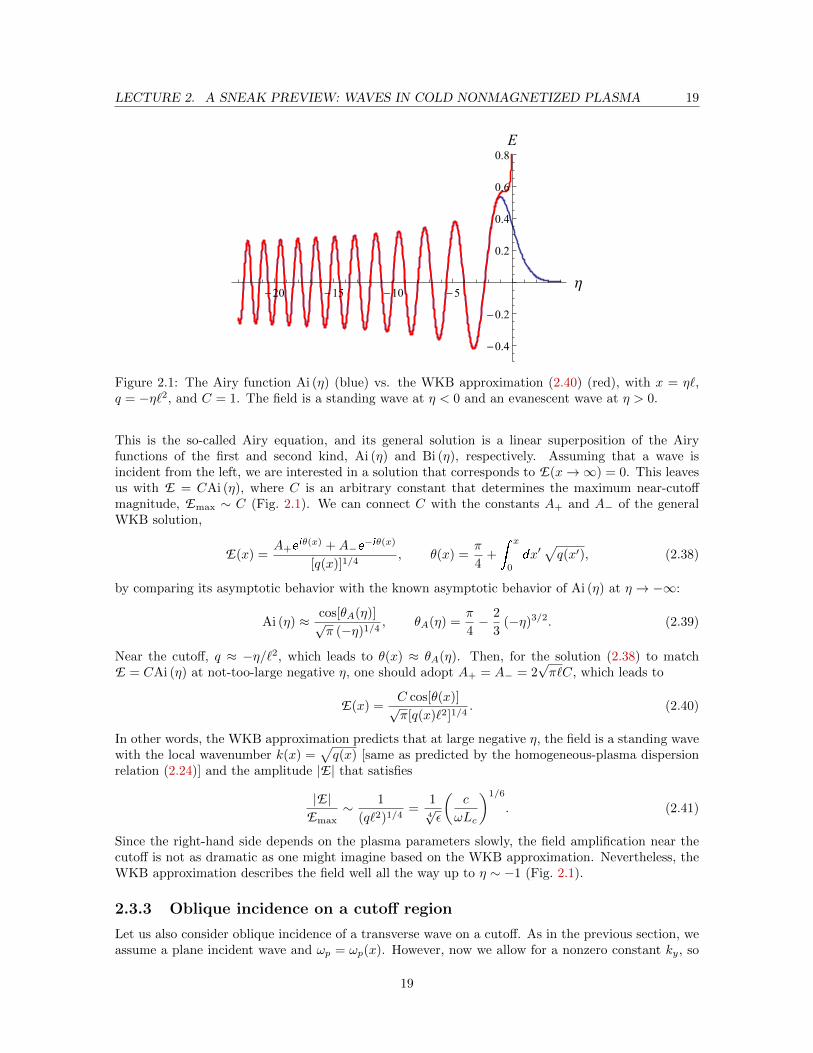
Figure 2.1: The Airy function Ai (η) (blue) vs. the WKB approximation (2.40) (red), with x = η`,q = −η`2, and C = 1. The field is a standing wave at η < 0 and an evanescent wave at η > 0.

This is the so-called Airy equation, and its general solution is a linear superposition of the Airyfunctions of the first and second kind, Ai (η) and Bi (η), respectively. Assuming that a wave isincident from the left, we are interested in a solution that corresponds to E(x→∞) = 0. This leavesus with E = CAi (η), where C is an arbitrary constant that determines the maximum near-cutoffmagnitude, Emax ∼ C (Fig. 2.1). We can connect C with the constants A+ and A− of the generalWKB solution,

E(x) =A+e

iθ(x) +A−e−iθ(x)

[q(x)]1/4, θ(x) =

π

4+

x

0

dx′√q(x′), (2.38)

by comparing its asymptotic behavior with the known asymptotic behavior of Ai (η) at η → −∞:

Ai (η) ≈ cos[θA(η)]√π (−η)1/4

, θA(η) =π

4− 2

3(−η)3/2. (2.39)

Near the cutoff, q ≈ −η/`2, which leads to θ(x) ≈ θA(η). Then, for the solution (2.38) to matchE = CAi (η) at not-too-large negative η, one should adopt A+ = A− = 2

√π`C, which leads to

E(x) =C cos[θ(x)]√π[q(x)`2]1/4

. (2.40)

In other words, the WKB approximation predicts that at large negative η, the field is a standing wavewith the local wavenumber k(x) =

√q(x) [same as predicted by the homogeneous-plasma dispersion

relation (2.24)] and the amplitude |E | that satisfies

|E |Emax

∼ 1

(q`2)1/4=

14√ε

(c

ωLc

)1/6

. (2.41)

Since the right-hand side depends on the plasma parameters slowly, the field amplification near thecutoff is not as dramatic as one might imagine based on the WKB approximation. Nevertheless, theWKB approximation describes the field well all the way up to η ∼ −1 (Fig. 2.1).

2.3.3 Oblique incidence on a cutoff region

Let us also consider oblique incidence of a transverse wave on a cutoff. As in the previous section, weassume a plane incident wave and ωp = ωp(x). However, now we allow for a nonzero constant ky, so

19


Box 2.1: Reinstating the WKB approximation near cutoffs

In principle, the WKB approximation can be reinstated near a cutoff by changing the represen-tation of the field equation. For example, consider the Airy equation (2.37) in the operator form,k2E + xE = 0. In the usual, coordinate representation, one has x = x and k = −i∂x. (Here, weblur the distinction between the dimensionless η and −i∂η on one side and the dimensional x and−i∂x on the other side for simplicity.) However, we can adopt the wavevector representation (cf.momentum representation in quantum mechanics), i.e., take the Fourier transform of the Airyequation. Then, x = i∂k and k = k, so the equation becomes

k2E + i∂kE = 0,

where E is the Fourier spectrum of E . This new equation can be solved using the WKBmethod. In fact, the corresponding WKB approximation, E = const × exp(ik3/3), is an exactsolution. Mapping it back to the coordinate space is only a matter of calculating the integraldk exp(ikx+ ik3/3), which can be done at various levels of accuracy.

One can also use a more general class of transforms called metaplectic transforms. The lattercan rotate (more generally, perform symplectic transformations of) the “phase space” (x, k)such that in the new phase space (x′, k′), the wavenumber k′ is never zero and thus cutoffs areeliminated [13] (Fig. 2.2). The Fourier transform can be considered as a particular case of themetaplectic transform that corresponds to 90 rotation.

the electric and magnetic fields can be written as follows:

E = Re [EEEEE(x)e−iωt+ikyy], B = Re [BBBBB(x)e−iωt+ikyy]. (2.42)

Two distinct wave patterns can be formed in this case, depending on the wave polarization. Below,we briefly discuss both cases.

TE wave

Let us start with the transverse-electric (TE) polarization (Fig. 2.3), which corresponds to Ex = Ey =

0. Since ∂zEz = 0, one has ∇ · E = 0, which leads to the following equation for Ez:

0 = ∇2Ez +ω2

c2ε(ω;x)Ez =

d2Ez

dx2+

1

c2[ω2 − c2k2

y − ω2p(x)]Ez. (2.43)

This equation is similar to Eq. (2.27) up to replacing ω2 → ω2− c2k2y. Thus, the field forms the same

WKB/Airy profile (Fig. 2.1), except the cutoff is shifted to the location where ω2p(x) = ω2 − k2

yc2, in

agreement with the homogeneous-plasma dispersion relation (2.24).

TM wave

Let us also consider the transverse-magnetic (TM) polarization (Fig. 2.3). In this case, ∇ · E isnonzero, which means that a transverse wave is coupled to the oscillations of the charge density, ρ,through Gauss’s law (1.1c). Similarly, ρ is coupled to E via (Exercise 2.4)

∂2t ρ+ ω2

pρ = f , f = − e2

me∇n0e · E. (2.44)

Equation (2.44) can be understood as the electrostatic wave equation for free Langmuir oscillationsdriven by an external force f ∝ E. If this force has a resonant frequency ω = ±ωp, the magnitude ofρ can become large. Then, several scenarios are possible.

20


Figure 2.2: An illustration of cutoff elimination using the metaplectic transform (Box 2.1): the phasespace is continuously transformed such that the wavenumber remains constant and thus a wave neversees a cutoff in this transforming frame. In the simplest case, the transformation is a rotation by somenonzero angle α, with α = 90 corresponding to the Fourier transform.

Figure 2.3: A schematic of transverse-wave oblique incidence on plasma with background electrondensity n0e = n0e(x) illustrating the difference between a TE wave and a TM wave. The vertical redline indicates the critical-density region, where ω2

p(x) = ω2. The dashed red line indicates the cutoffregion, where ω2

p(x) = ω2 − k2yc

2. Waves are propagating on the left and evanescent on the right.The background color intensity illustrates the background density, with darker colors correspondingto higher densities.

21


0x

Ex

Figure 2.4: A typical Ex [Eq. (2.46), numerical solution] for intermediate β and weak dissipation,with the boundary conditions corresponding to vanishing Bz at x → ∞. Here, ε(ω;x) is given byEq. (2.18), with ω2

p(x) given by Eq. (2.36).

When the angle β between k and ∇n0e approaches zero, one recovers the usual WKB/Airy profilediscussed above. Likewise, if β is large, one can expect from Eq. (2.24) that the wave is reflectedmuch earlier than it reaches the critical-density region. Then, f is extremely small in the resonanceregion, so Langmuir oscillations are not excited (unless the collision rate is also extremely small) anda TM wave behaves just like a TE wave. However, at intermediate β, the coupling of a TM wave withLangmuir oscillations can be substantial and results in a significant peak of the wave field near thecritical region. This can be described by the following equations (Exercise 2.4)

d2Bz

dx2− ∂ ln ε(ω;x)

∂x

dBz

dx+

[ω2

c2ε(ω;x)− k2

y

]Bz = 0, (2.45)

Ex = − ckyBz

ωε(ω;x), Ey =

ic

ωε(ω;x)

dBz

dx. (2.46)

A typical Ex [Eq. (2.46)] for intermediate β is shown in Fig. 2.4, where the Airy pattern is seen on theleft and a large near-singular field is seen near the Langmuir resonance. (For details and asymptoticanalytic solutions, see Ref. [14].) Note that a small collision rate has to be added to keep the wavefield finite. This is due to the fact that energy is continuously deposited by the incoming wave intoLangmuir oscillations and cannot escape the critical-density region, because Langmuir waves are tiedto this region and because they cannot dissipate collisionlessly in cold plasma. One can show thatadding thermal effects removes both these limitations.

The coupling of TM waves with Langmuir oscillations is an example of mode conversion, which ismathematically similar to quantum tunneling. Note that this effect is completely missed within thehomogeneous-plasma analysis (Sec. 2.2), where the two transverse modes have identical propertiesand are completely uncoupled from Langmuir oscillations. To capture polarization effects robustlyand in a general geometry, a more systematic theory is needed. Later, we will present such theory,which will be readily applicable to almost any dispersion operators.

Exercise 2.4: Derive Eqs. (2.44)–(2.46).

22

Appendices for Part I

AI.1 Analytic properties of response functions

Here, we briefly summarize some important properties of response functions that commonly emergein theory of dispersion. We will be concerned only with temporal dynamics, so possible dependenceof these functions on spatial coordinates and wavevectors will be ignored.

Let us consider a general system whose response j (which may or may not be the current density)to an external force E (which may or may not be the electric field) is linear, i.e., can be expressed interms of some Green’s function Σ:

j(t) =

t

0

dt′ Σ(t− t′)E(t′). (2.47)

Let us assume that our system is stable in the sense that a response to a delta-shaped field eventuallyfades away, i.e., Σ(t→ +∞) = 0.5 Then, the integral that determines its Laplace image,

σ(ω) =

∞0

dt e iωtΣ(t), (2.48)

converges for all ω that satisfy Imω ≥ 0. Similarly, if Σ(t) fades away faster than any power of t att→∞ (which is typically the case, as discussed in Lecture 8), then all integrals of the form

Jn[Σ](ω).=

∞0

dt e iωt(it)nΣ(t) (2.49)

converge too. [The square brackets denote that Jn is a functional of Σ, and (ω) denotes that Jndepends on ω, as usual.] Since Jn[Σ](ω) = σ(n)(ω), where (n) is the nth derivative, this means thatall derivatives of σ(ω) are well defined at Imω ≥ 0. This proves the following theorem:

Theorem: σ(ω) is analytic in the upper half of the complex-ω plane.

Next, note that the function σ(ω) ≡ J0[Σ](ω) =∞

0dt e iωtΣ(t) can be expressed as follows:

J0[Σ](ω) =

∞0

dt

d

dt

[e iωt

iωΣ(t)

]− e iωt

iωΣ′(t)

=

1

iω

[eiωtΣ(t)

] ∣∣∞0− 1

iω

∞0

dt e iωtΣ′(t)

= − Σ(0)

iω− J0[Σ′](ω)

iω. (2.50)

5This does not rule out collective instabilities, where the field itself grows in time. In the sense assumed here, theresponse of a current to an external field, which is described by the conductivity operator σ, is typically stable. (Systemsexhibiting avalanche ionization are exceptions.) In contrast, the response of a self-consistent field to an external current,which is described by D−1

E , is often not.

23

APPENDICES FOR PART I 24

[Here, we have assumed that the function Σ is also sufficiently well behaved so that Σ(0) and J [Σ′] arefinite.] The function Σ(t) is determined by microscopic processes that have some nonzero minimumtime scale T . Then, roughly, |J [Σ′]| . |J [Σ]|/T . Hence, at ω T −1, the second term on the right-hand side of Eq. (2.50) can be neglected compared to the term on the left-hand side. Thus, at largeenough ω, one has σ(ω) ≈ iΣ(0)/ω, and in particular,

σ(ω →∞) = 0. (2.51)

In combination with Eq. (2.51), the analyticity of σ(ω) in the upper half of the complex-ω plane(proven above) leads to some interesting properties of the functions

σr (ω).= Reσ(ω), σi (ω)

.= Imσ(ω). (2.52)

These properties are derived as follows. Let us consider real ω0 and the integral

I(ω0).=

C

dωσ(ω)

ω − ω0, (2.53)

where C is a contour that goes along the real axis and encircles the pole at ω = ω0 from above. Onone hand, one can rewrite I(ω0) as

I(ω0) =

∞−∞

dωσ(ω)

ω − ω0− iπσ(ω0), (2.54)

where

denotes the Cauchy principal value of the corresponding integral. On the other hand, onecan close the contour C through a semicircle C+ with radius R→∞ at Imω > 0, because the integralover C+ is zero. [This is because at ω →∞, the integrand decreases faster than 1/ω due to σ(ω)→ 0.]But σ(ω)/(ω − ω0) is analytic everywhere within the closed contour, so the integral over this closedcontour must be zero. Therefore, I(ω0) = 0, which means

σ(ω0) = − i

π

∞−∞

dωσ(ω)

ω − ω0. (2.55)

By taking the real and imaginary parts of Eq. (2.55), one obtains that σr and σi are connected viathe Hilbert transform; namely,

σr (ω0) =1

π

∞−∞

dωσi (ω)

ω − ω0, (2.56a)

σi (ω0) = − 1

π

∞−∞

dωσr (ω)

ω − ω0. (2.56b)

These are known as the Kramers–Kronig relations. They show that having nonzero σi at some frequen-cies implies having nonzero σr at some (possibly, different) frequencies, and vice versa. Notably, thecollisionless dissipation discussed in Part IV can be anticipated from the Kramers–Kronig relations.

24

Problems for Part I

PI.1 Electrostatic approximation

In some cases, a wave can be considered electrostatic, meaning that its electric field is approximatelyrepresentable as (minus) the gradient of an electrostatic potential, E ≈ −∇ϕ. Such waves can beeasier to describe, because instead of the multiple components of E, one can work with a singlefunction ϕ. Here, you are asked to explore the electrostatic-wave approximation for a homogeneousstationary medium.

(a) Consider the components of E parallel and perpendicular to the wavevector, E‖ and E⊥. UsingEq. (1.36), estimate the ratio of |E‖| and |E⊥| at sufficiently large N and argue that

N2 εab for all a and b (2.57)

is a sufficient condition for a wave to be electrostatic.

(b) Assuming that the field is electrostatic and that the medium is described by an unspecifieddielectric tensor ε, derive the corresponding dispersion relation from Gauss’s law. Show that thesame result is obtained from Eq. (1.36) if one takes for granted that the field is electrostatic.

(c) In a gyrotropic medium with no spatial dispersion, the dielectric tensor has the form

ε(ω,k) =

ε⊥(ω) −ig(ω) 0ig(ω) ε⊥(ω) 0

0 0 ε‖(ω)

. (2.58)

Consider an electrostatic wave propagating with a such medium with k = k⊥, 0, k‖. (One canalways choose axes such that ky = 0.) Substitute this k and Eq. (2.58) for ε into the dispersionrelation derived in problem (b). Using your result, show that the group velocity of such a waveis orthogonal to the wave phase velocity.

PI.2 Photon wave function in cold magnetized plasma

Consider a cold plasma formed by N species with charges es, masses ms, and unperturbed densitiesn0s = n0s(x). Assume that this plasma is immersed in a stationary magnetic field B0(x) and has noaverage flows.

(a) Show that the combination of the linearized momentum equation for the fluid velocities vs,Ampere’s law for the wave electric field E, and Faraday’s law for the wave magnetic field E canbe represented together in the form

i∂tψ = Hψ, (2.59)

25

PROBLEMS FOR PART I 26

or equivalently, Dψψ = 0 with Dψ = ω − H, where ψ is a 3(N + 2)-dimensional real vectorfield (the same equation can be expressed without i) and the Hamiltonian H being the followingHermitian operator:

H =

−α ·Ω1(x) 0 . . . 0 iωp1(x) 00 −α ·Ω2(x) . . . 0 iωp2(x) 0...

.... . .

......

...0 0 . . . −α ·ΩN (x) iωpN (x) 0

−iωp1(x) −iωp2(x) . . . −iωpN (x) 0 icα · k0 0 . . . 0 −icα · k 0

. (2.60)

Here, Ωs.= esB0(x)/(msc), ωps

.= es

√4πn0s(x)/ms (note that this definition is slightly differ-

ent from the one that we used earlier), and α.= (αx, αy, αz)

ᵀ is the column vector comprised ofthe following Hermitian matrices:6

αx.=

0 0 00 0 −i0 i 0

, αy.=

0 0 i

0 0 0−i 0 0

, αz.=

0 −i 0i 0 00 0 0

. (2.61)

Note that Eq. (2.59) is similar to the Schrodinger equation for vector particles. (This becomeseven more evident if one multiplies it by ~ and expresses the right-hand side through the mo-mentum operator p

.= ~k instead of the wavevector operator k.) Thus, ψ can be understood as

the photon wave function in cold plasma (cf. the photon wave function in vacuum [15]).

Hint: Use ψ = (ζ1, ζ2, . . . , ζN , E, B)ᵀ, where ζs is a rescaled vs, with the rescalingfactor that you are asked to find. Also use that for any three-component columnvectorsA and B, one hasA×B = −i(α·A)B, as can be verified by direct calculation.

(b) Calculate |ψ|2, which is the same as ψ2 here. What is the physical meaning of this quantity?Show that

dx |ψ(t,x)|2 ≡ 〈ψ|ψ〉 is conserved.

Hint: In the last question, use Eq. (2.59) and the fact that H is Hermitian. Do notuse the explicit formula (2.60), or your calculations will be much longer than necessary.

(c) Argue that cold-plasma modes governed by Eq. (2.59) cannot be unstable, irrespective of howinhomogeneous the plasma and B0 are.7

Hint: This can be argued in one sentence.

PI.3 Beam–plasma instability (cold electrostatic limit)

Consider one-dimensional nonmagnetized collisionless cold homogeneous stationary electron plasmawith motionless ions. Suppose that bulk electrons have the average density n0 and zero averagevelocity. Consider also a cold electron beam with some average density nb and some average velocity vb.

(a) Consider bulk electrons and beam electrons as different species. Show that the beam-electronsusceptibility in the spectral representation is given by χb(ω, k) = −ω2

b/(ω − kvb)2, where ωb.=√

4πnbe2/me. (You may adopt ω = ω and k = k.)

6Notably, αa belong to the family of Gell–Mann matrices, which serve as infinitesimal generators of SU(3).7This is true only for cold plasma without flows. Otherwise, H is different and generally has different properties.

26

PROBLEMS FOR PART I 27

(b) Calculate the plasma dielectric function ε(ω, k) and write down the general dispersion relationof electrostatic oscillations.

(c) How many branches does this dispersion relation have?

(d) Show graphically, by qualitatively analyzing the function ε(ω, k) derived in (b) and using youranswer from (c), that such plasma is unstable at small enough k.

(e) For the unstable regime, plot Reω and Imω as functions of k. (You may do it qualitatively orby solving the dispersion relation numerically, but make sure to plot all branches.)

(f) Assuming η.= nb/n0 is a small parameter, show that the maximum of the growth rate γ scales

as γmax ∝ η1/3. (If a beam is warm, which case will be studied later in this course, the scalingfor γ can be different.)

Hint: Use the fact that, to the zeroth order in η, the unstable branch has ω = kvb[as you should be able to see from (e)]. Show that to the leading order, γ → ∞ atk = ±ωp0/vb, where ω2

p0.=√

4πn0e2/me. Hence, adopt k = ±ωp0/vb as the optimumwavenumber for the instability and then find γ more accurately.

PI.4 Surface waves

Here, you are asked to study azimuthally symmetric electromagnetic waves propagating along a cold-plasma column of finite radius a. Assume the cylindrical coordinates (r, θ, z), where z is the axis ofsymmetry, and E = Re (EEEEE e−iωt+ikzz), with constant ω and kz. For simplicity, consider only TMwaves, i.e., waves with Bz = 0.

Hint: Remember that the tangential component of the electric field is always continuousat the plasma boundary. Make sure you understand why.

(a) Using Maxwell’s equations for the three components of the electric field E and the three com-ponents of the magnetic field B, show that the above assumptions lead to Eθ = Br = Bz = 0at r 6= a. (Assume that ε 6= 0.) Argue that in this problem, Bθ is continuous at the plasmaboundary.

(b) Show that ∇ · E = 0 at r 6= a. Using this, show that Ez satisfies the modified Bessel equation

d2Ez

dζ2+

1

ζ

dEz

dζ− Ez = 0. (2.62)

Here ζ.= κr, κ2 .

= k2z+ω2

p/c2−ω2/c2, ωp(r < a) = ωp0 is a nonzero constant, and ωp(r > a) = 0.

Using the continuity of Ez at r = a, find Ez(r) as a piecewise-analytic function. (Rememberthat your solution is supposed to be finite everywhere, including r → 0 and r →∞.)

(c) Using the continuity of Bθ at r = a (which can be expressed through dEz/dζ), show that thedispersion relation is (

1−ω2p

ω2

)1

κina

I1(κina)

I0(κina)+

1

κouta

K1(κouta)

K0(κouta)= 0. (2.63)

Here, In and Kn are modified Bessel functions of the first and second kind, respectively; also,κin

.= κ(r < a) and κout

.= κ(r > a).

(d) Solve Eq. (2.63) numerically. Plot ω(kz) and Ez(r) for several values of a/δc, where δp.= c/ωp0.

Explain the results qualitatively.

27

Part II

Basic theory ofquasimonochromatic waves

In this part of the course, we outline a general asymptotic theory of quasimonochro-matic waves in linear dispersive media. In the context of fusion research, our discussionis particularly relevant to waves in the electron-cyclotron and lower-hybrid ranges of fre-quencies, which correspond to mm and cm wavelengths, respectively (Part III). For waveswith longer wavelengths, such as those in the ion-cyclotron range, our discussion is relevantqualitatively.

28

Lecture 3

Asymptotic expansion of dispersionoperators

In this lecture, we derive an approximate envelope equation for a general quasimonochromatic waveby asymptotically expanding the wave dispersion operator. In doing so, we also introduce the Wigner–Weyl transform, which is a central element of modern wave theory and will be used also in other partsof the course.

3.1 Problem setup

Let us consider a general wave ψ governed by

Dψ = 0, (3.1)

where D is a linear dispersion operator. We will assume that the wave remains quasimonochromatic,so ψ can be split into a rapid real phase θ (“eikonal”, to be specified in Lecture 4) and a slow complexenvelope Ψ:

ψ = eiθΨ. (3.2)

Then, the quantities

w.= −∂tθ, k

.= ∇θ (3.3)

represent the local frequency and the local wavevector (note that they are real by definition), and

τ.=

2π

w, λ

.=

2π

k(3.4)

are the local temporal period and the local spatial period (wavelength). Suppose the characteristictemporal and spatial scales of Ψ, w, k, and of the medium are limited from below by some values Tcand Lc, respectively. Then, we introduce a “geometrical-optics parameter”

ε.= max

τ

Tc,λ

Lc

1. (3.5)

Our goal is to develop an approximate geometrical-optics (GO)1 theory that captures the leading-order effects caused by nonzero ε. This will be done by approximating the dispersion operator D tothe first order in ε, which involves three main steps:

1The name “GO” is determined by the fact that the regime ε 1 was initially studied for optical waves. Higher-ordertheories include the quasioptical approximation and the paraxial approximation as a special case (Box 3.1).

29

LECTURE 3. ASYMPTOTIC EXPANSION OF DISPERSION OPERATORS 30

(i) map the operator D to some function D,

(ii) approximate the function D using ε as a small parameter,

(iii) and map the approximated function back to the operator space.

To ensure that D be efficiently expandable in ε, the mapping will be done using the Wigner–Weyltransform (WWT).2 But let us introduce some basic notation first.

3.2 Notation

To shorten the calculations, we will describe the wave propagation in terms of spacetime coordi-nates xα, or in the invariant notation, x = x0,x, where x0 .

= ct and xa with a > 0 are spatialcoordinates. The dimension of the coordinate space n

.= dimx can be any n ≥ 0. The spacetime

dimension is n.= dim x = n + 1 and restricted to n ≥ 1. For simplicity, we restrict our consideration

to spacetimes Mn with the Minkowski metric gαβ = gαβ = diag −1, 1, 1, . . ..3 Then, w and k can beexpressed through the components of the row vector

kα.= −∂αθ = (−w/c, k)α, (3.6)

where ∂α.= ∂/∂xα; in particular, k0 = −w/c. The corresponding column vector has components

kα = gαβkβ , where gαβ is the inverse metric. In case of the Minkowski metric, gαβ = gαβ , sok0 = −k0 = w/c and ka = ka, or in the invariant form, k = (w/c, k)ᵀ. This implies

k · x = gαβ kαxβ = kαx

α = −k0x0 + kaxa = −wt+ k · x. (3.7)

The operators ω.= i∂t and k

.= −i∇ that we introduced earlier can be similarly expressed through

kα.= −i∂α. (3.8)

By analogy with quantum mechanics, let us consider scalar fields on Mn as vectors |ψ〉 in thecorresponding Hilbert space. Then, any scalar function ψ(x) can be understood as the x-representationof the corresponding vector |ψ〉; namely, ψ(x′) = 〈x′|ψ〉. Here, |x′〉 is the normalized eigenvector ofthe coordinate operator x that corresponds to the eigenvalue x′; i.e.,

x |x′〉 = x′ |x′〉 , 〈x′|x′′〉 = δ(x′ − x′′), (3.9)

sodx′ |x′〉〈x′| is a unit operator. (All integrals are taken on (−∞,+∞) unless specified otherwise.)

Accordingly, any (Mψ)(x) can be expressed as

(Mψ)(x) = 〈x|Mψ〉 ≡ 〈x|M |ψ〉 =

dx′ 〈x|M |x′〉〈x′|ψ〉 =

dx′M(x, x′)ψ(x′), (3.10)

where M(x, x′).= 〈x|M |x′〉 is the x-representation of M . Similarly, one can introduce the normalized

eigenvectors of the wavevector operator k,

k |k′〉 = k′ |k′〉 , 〈k′|k′′〉 = δ(k′ − k′′), (3.11)

and define the k-representation of vectors as 〈k|ψ〉 and of operators as 〈k|M |k′〉 (Exercise 3.1).

2Reported here is a modern approach to GO [16, 17]. Earlier formulations of GO [18] do not use the term WWTexplicitly but still follow similar steps.

3Readers who are not familiar with tensor analysis may consider upper-index and lower-index quantities as indepen-dent functions formally defined through the formulas below.

30


Exercise 3.1: Show that 〈x|k〉 = 〈k|x〉∗ = (2π)−n/2e ik·x.

For N-component vector fields

ψ =

ψ1

ψ2

. . .ψN

, (3.12)

where ψu are scalar fields on Mn and N may or may not coincide with n, we similarly introduce

|ψ〉 =

|ψ1〉|ψ2〉. . .|ψN〉

(3.13)

via ψu(x′) = 〈x′|ψu〉. Then, operators on vector fields are considered as matrices of operators that acton the field components; i.e.,

(Muvψv)(x) =

dx′Muv(x, x

′)ψv(x′), Muv(x, x

′) = 〈x|Muv|x′〉 , (3.14)

the k-representations of matrix operators are introduced similarly.

3.3 Wigner–Weyl transform

The WWT4 can be understood as a “mixed”, or “phase-space”, representation of an operator. Unlikethe x- and k-representations, which involve projections either on |x〉 or on |k〉, the WWT projects anoperator on both |x〉 and |k〉 simultaneously. In a nutshell, the WWT maps M to a linear combinationof 〈x|M |k〉 and 〈k|M |x〉 with all possible x and k and the coefficients such that this mapping has“natural” properties. This is more easily seen from the definition of the WWT that is formulated interms of the “phase-space” coordinates z

.= x, k [2, 19, 20]. Here, though, we will use a less elegant

definition that is perhaps easier to absorb. This definition is as follows.For any given scalar operator M , its Weyl image M(x, k) ≡ W [M ], also called the (Weyl) symbol

of M , is a function defined on the 2n-dimensional real space (x, k) as follows:

M(x, k).=

ds 〈x + s/2|M |x− s/2〉 e−ik·s. (3.15)

One can also understand M(x, k) as the Fourier image of M(x, s).= M(x + s/2, x − s/2) with respect

to s at fixed x = x (cf. Box 1.1):

M(x, k) =

ds M(x, s) e−ik·s. (3.16)

The inverse WWT4 W −1 maps any given function M(x, k) to an operator M via [19]

M =1

(2π)n

dx dk ds |x + s/2〉M(x, k) e ik·s 〈x− s/2| . (3.17)

4The direct WWT is also called the Wigner transform. The inverse WWT is also called the Weyl transform.

31


For M that is a matrix of operators Muv, the corresponding symbol M(x, k) is defined as the matrixwhose elements are the symbols of Muv. Also note that the WWT commutes with the Hermitianconjugation:

W [M†] = M†(x, k). (3.18)

As a corollary (Problem 3.2), the Hermitian and anti-Hermitian parts [Eq. (C.3)] of M and M satisfy

MH(x, k) = W [MH], MA(x, k) = W [MA]. (3.19)

Exercise 3.2: Prove Eqs. (3.18) and (3.19). Show that the symbol of a Hermitian operator is aHermitian matrix or, in case of a scalar operator, a real function.

The WWT is a natural mapping between operators and functions on phase space in the followingsense. The symbol of a unit operator is unity:

W [1] =

ds 〈x + s/2|1|x− s/2〉 e−ik·s

=

ds 〈x + s/2|x− s/2〉 e−ik·s

=

ds δ(s) e−ik·s

= 1. (3.20)

The symbol of an operator that can be represented as a function of the coordinate operator x is thesame function of x:

W [F (x)] =

ds 〈x + s/2|F (x)|x− s/2〉 e−ik·s

=

dsF (x− s/2) 〈x + s/2|x− s/2〉 e−ik·s

=

dsF (x− s/2)δ(s) e−ik·s

= F (x). (3.21)

Similarly, the symbol of an operator that can be represented as a function of the wavevector operatork is the same function of k (Exercise 3.3):

W [G(k)] =

ds 〈x + s/2|G(k)|x− s/2〉 e−ik·s = G(k). (3.22)

Also, the symbol of an operator representable as F (x) +G(k) is F (x) +G(k). In summary then,

1⇔ 1, x⇔ x, k⇔ k, F (x) +G(k)⇔ F (x) +G(k), (3.23)

where ⇔ denotes the correspondence between operators and their symbols.

Exercise 3.3: Prove Eq. (3.22) using the result from Exercise 3.1.

32


In the general case, though, the correspondence ⇔ is more complicated than swapping (x, k) and(x, k). For example,

W [kF (x)] =

ds e−ik·s 〈x + s/2|kF (x)|x− s/2〉

=

dk′ ds e−ik·s 〈x + s/2|k′〉 kF (x− s/2) 〈k′|x− s/2〉

=

dk′ ds e−ik·s 〈x + s/2|k′〉 k′F (x− s/2) 〈k′|x− s/2〉

=

dk′

(2π)nds k′F (x− s/2) e i(k

′−k)·s

=

dk′

(2π)nds (k′ + k)F (x− s/2) e ik

′·s

= k

dk′

(2π)ndsF (x− s/2) e ik

′·s − i

dk′

(2π)ndsF (x− s/2) ∂se

ik′·s

= k

dsF (x− s/2)δ(s) + i

dk′

(2π)nds ∂s[F (x− s/2)] e ik

′·s

= kF (x)− i

2∂x

dk′

(2π)ndsF (x− s/2) e ik

′·s

= kF (x)− i

2∂xF (x). (3.24)

Using Eq. (3.18), one also obtains

W [F (x)k] =(W [(F (x)k)†]

)†=(W [kF †(x)]

)†=[kF †(x)− i/2 ∂xF

†(x)]†

= F (x)k + i/2 ∂xF (x), (3.25)

and as a corollary,

kF (x), F (x)k ⇔ 1/2 [F (x)k + kF (x)] . (3.26)

The terms ∂αF in Eqs. (3.24) and (3.25) emerge because x and k do not commute,

[xα, kβ ] = iδαβ . (3.27)

These terms are of order ε and vanish in the GO limit (ε→ 0). Similarly, for a general M = M (0)(x, k),where M (0) is any combination of x and k, one has

W [M ] = M (0)(x, k) +O(εM (0)

). (3.28)

3.4 Envelope equation

Now, let us return to Eq. (3.1), multiply it by e−iθ(x), and rewrite the result as follows:

DΨ = 0, D .= e−iθ(x)D e

iθ(x). (3.29)

The operator D serves as the envelope dispersion operator and can also be expressed in the followinginvariant form:

D = e−iθ(x)D e

iθ(x). (3.30)

33


By definition [Eq. (3.15)], the symbol of D is

D(x, k) =

ds 〈x + s/2|e−iθ(x)D e

iθ(x)|x− s/2〉 e−ik·s

=

ds 〈x + s/2|e−iθ(x+s/2)D e

iθ(x−s/2)|x− s/2〉 e−ik·s

=

ds 〈x + s/2|D|x− s/2〉 e−i [θ(x+s/2)−θ(x−s/2)+k·s]. (3.31)

Since the gradient of θ is assumed to be a slow function, we can use

θ(x± s/2) = θ(x)± sα

2

∂θ

∂xα+sαsβ

8

∂2θ

∂xα∂xβ± sαsβsγ

48

∂3θ

∂xα∂xβ∂xγ+ . . . , (3.32)

where summation over repeated indexes is assumed. Then,

e−i [θ(x+s/2)−θ(x−s/2)+k·s] =

(1− i

24sαsβsγ

∂2kγ∂xα∂xβ

+ . . .

)e−i [k(x)+k]·s

=

(1− 1

24

∂2kγ∂xα∂xβ

∂3

∂kα∂kβ∂kγ+ . . .

)e−i [k(x)+k]·s, (3.33)

where we assumed that the second term in the parentheses is small compared to one. (A more explicitestimate of the error is presented below.) This leads to

D(x, k) =

(1− 1

24

∂2kγ∂xα∂xβ

∂3

∂kα∂kβ∂kγ+ . . .

) ds 〈x + s/2|D|x− s/2〉 e−i [k(x)+k]·s

=

(1− 1

24

∂2kγ∂xα∂xβ

∂3

∂kα∂kβ∂kγ+ . . .

)D(x, k(x) + k

)= D′

(x, k(x) + k

), (3.34)

where we have introduced

D′(x, k).= D(x, k)− 1

24

∂2kγ∂xα∂xβ

∂3D(x, k)

∂kα∂kβ∂kγ+ . . . (3.35)

Note that the inverse WWT will, loosely speaking, turn the coordinate k into the operator k. Thelatter will act on the wave envelope, which is considered slow in the coordinate representation, sok |Ψ〉 = O(ε). In this sense, k = O(ε) in Eq. (3.34). Then, D′(x, k(x) + k) can be Taylor-expandedin k, which corresponds to expanding D in ε. Next, notice that

ε′.= D[x, k(x) + k]−1 ∂2kγ

∂xα∂xβ∂3D[x, k(x) + k]

∂kα∂kβ∂kγ

≈ D(x, k)−1 ∂2kγ∂xα∂xβ

∂3D(x, k)

∂kα∂kβ∂kγ

∼(

k

L2cD

)(D

k3

)= O(ε2), (3.36)

where we have assumed ∂/∂xα ∼ 1/Lc and ∂/∂k ∼ 1/k.5 Because we are interested only in O(ε)corrections, this means that on the right-hand side of Eq. (3.35), the second term can be neglected

5A more accurate estimate is as follows. Let us consider D(x, k) in the form (3.16), i.e., D(x, k) =ds D(x, s) e−ik·s.

Then, ∂D/∂kα = −ids D(x, s)sαe−ik·s ∼ sαD, where sα is the characteristic scale on which D(x, s) fades away along

the sα axis. Then, ε′ ∼ (kLc)−2(ks)3 ∼ ε2(ks)3. To ensure that ε′ ε, one must require (ks)3ε 1. Strictlyspeaking, this is an additional requirement of GO, independent of Eq. (3.5). The scale s can be estimated in thehomogeneous-plasma limit, when D(x, k) is just the dispersion tensor, D(x, k)→D(k).

34


Box 3.1: Quasioptical and paraxial approximation

In practice, waves often propagate as narrow beams whose transverse scale L⊥ is much less thanthe longitudinal scale L‖, which is comparable to that of the medium. For diffraction-limitedbeams, one has ε‖ ∼ ε2

⊥, where ε‖.= (kL‖)

−1 and ε⊥.= (kL⊥)−1, so when retaining terms of the

first order in ε‖, one must retain effects of the second order in ε⊥. Because ε′ [as in Eq. (3.36)] isof order ε2

‖, Eq. (3.37) is still applicable, but Eq. (3.38) must be replaced with the second orderexpansion in k⊥. The corresponding envelope equation is

D[x, k(x)

]Ψ− i

2(∂αVα)Ψ− iVα∂αΨ− 1

2(Φαβ : ∇⊥α∇⊥β)Ψ = 0,

where Φαβ.= ∂2D/∂kα ∂kβ evaluated at [x, k(x)]. This model is called the paraxial approximation

if the beam axis is a straight line, or in the general case, the quasioptical approximation [17]. It iswidely used, for example, in optics and also for modeling mm- and cm-wave beams in magneticallyconfined plasmas.

compared to the first term. In other words, D′(x, k) ≈D(x, k) and thus

D(x, k) ≈D(x, k(x) + k

), (3.37)

or using first-order Taylor expansion,

D(x, k) ≈D(x, k(x)

)+ kαVα(x), Vα(x)

.=

(∂D(x, k)

∂kα

)k=k(x)

. (3.38)

By Eq. (3.26), the inverse WWT of this expression is

D ≈D(x, k(x)

)+

1

2[kαVα(x) + Vα(x)kα], (3.39)

or in the coordinate representation,

DΨ ≈D(x, k(x)]Ψ(x)− i

2∂α[Vα(x)Ψ(x))− i

2Vα(x)∂αΨ(x). (3.40)

Then, the envelope equation DΨ = 0 can be approximately expressed as follows:

D(x, k(x)

)Ψ− i

2(∂αVα)Ψ− iVα∂αΨ = 0, (3.41)

which can be considered as an extension of Eq. (1.52) to a general inhomogeneous medium (Box 3.1).We will further simplify this equation in Lecture 4.

3.5 How to use the envelope equation

In order to use Eq. (3.41), one must knowD to the first order in ε, which can be challenging to calculatein practice. Fortunately, this problem is often alleviated by the following. As seen from Lecture 2 andProblem PI.2, collisionless cold static (CCS) plasmas are naturally described by Hermitian dispersionoperators that satisfy (Exercise 3.4)

DCCS = D(0)CCS, (3.42)

35


where the notation is the same as in Sec. 3.3. Deviations from CCS models due to thermal effects andcollisions often result in only small corrections ∆ to the dispersion operator D. Then, the symbol ofthis operator, D, satisfies

D −D(0) =(DCCS + ∆

)−(D

(0)CCS + ∆(0)

)= ∆−∆(0) = O(ε∆), (3.43)

where we have used Eq. (3.28) to obtain the last equality. Because both ε and ∆ are small, the termO(ε∆) is often negligible [as opposed to O(ε) and O(∆)], i.e., one can adopt

D ≈D(0). (3.44)

This means that the symbol of the dispersion operator can be approximated with the dispersion tensorof homogeneous plasma. In fact, the two are often not even distinguished explicitly in literature.

Exercise 3.4: Calculate the symbols of: (a) DE for waves in CCS nonmagnetized plasma(Lecture 2) and (b) Dψ for waves in CCS magnetized plasma (Problem PI.2).

Because D(0)CCS is Hermitian, Eq. (3.44) is often further reduced to (Box 3.2)

DH ≈D(0)CCS + ∆

(0)H ≈D(0)

CCS, DA ≈ 0 + ∆(0)A = ∆

(0)A . (3.45)

This is justified in the following sense. In DH, which determines wave propagation (Lecture 5), themain contribution is provided by DCCS, so ∆H is only a small correction, which is often negligible.In contrast, DA, which determines wave dissipation (Lecture 5), is entirely determined by ∆A, sounlike ∆H, the function ∆A must be kept. The advantage of the model (3.45) is that D

(0)CCS (Part III)

is simpler than D(0)H (Part IV) and thus easier to implement numerically. (However, note that this

model can be insufficient when dissipation is strongly inhomogeneous. Sometimes this happens forresonant absorption, which is naturally localized in space.)

The arguments presented in this section do not apply to corrections ∆m caused by plasma motion.In this case, ∆

(0)m = 0, so Eq. (3.43) becomes D −D(0) = ∆m = O(ε). Ignoring this correction can

lead to significant violation of energy conservation on times t = O(ε−1) and is typically not acceptable.One must actually recalculate the dispersion operator for moving plasma to fix this issue. (But if oneneeds an equation just for the energy, the problem can be bypassed as discussed in the next lectures.)This asymmetry in how GO tolerates various corrections is due to the fact that plasma temporaldispersion is typically much stronger than plasma spatial dispersion.

36


Box 3.2: Subtleties with approximating D in other formulations of GO

Although GO can be constructed based on a transform other than the WWT, the approxima-tion (3.45) relies on the WWT property (3.19) that the other transform may not have. Then,one might not be able to approximate the corresponding symbol of D with the (well-known)dispersion tensor of the wave in a homogeneous medium.

For example, sometimes GO is constructed based on the transform

W [M ].=

dsM(x, x− s) e−ik·s =

〈x|M |k〉〈x|k〉

(e.g., see Ref. [21]). To the extent that the commutator [x, k] is negligible, one has W [M ] ≈M (0)(x, k), so W satisfies Eq. (3.28) just like the WWT. However, symbols produced by thetransform W do not have the property (3.18). As a result,

(W [D])A = D(0)A + [O(εD(0))]A = D

(0)A +O(ε).

Both terms on the right-hand side are of the same order, so the anti-Hermitian part of the symboldiffers from the corresponding matrix in homogeneous plasma by ∼ ∂2D

(0)H /∂xα∂kα. This leads

to alternative GO equations, which often results in confusion and stirred a controversy [22,23].

37

Lecture 4

Equations of geometrical optics

In this lecture, we derive a complete set of equations that describe scalar waves: the local dispersionrelation, the polarization equation, the consistency relations, the ray equations, and scalar-amplitudeequations, including an equation for the wave action. These are known as the equations of GO.

4.1 Scalar-wave model

Based on the reasoning presented in Sec. 3.5, let us assume the following ordering:

DH(x, k) = O(1), DA(x, k) = O(ε). (4.1)

Then, since ∂α = O(ε) and DA = O(ε), the envelope equation (3.41) can be simplified as follows:

DH

[x, k(x)

]Ψ + iDA

[x, k(x)

]Ψ− i

2(∂αVαH)Ψ− iVαH∂αΨ = 0, (4.2)

where VαH is the Hermitian part of Vα. It is readily seen from here that

DH[x, k(x)]Ψ = O(ε). (4.3)

This means that the field polarization must approximately satisfy the same equation as in the cor-responding homogeneous medium, DH[x, k(x)]Ψ ≈ 0. Hence, it is convenient to represent Ψ in thebasis of the orthonormal eigenvectors hv(x) of DH[x, k(x)],

Ψ(x) =

N∑v=1

hv(x)Ψv(x), hu · hv ≡ h†u(x)hv(x) = δuv (4.4)

(as earlier, N.= dim Ψ), and the corresponding eigenvalues Λv(x), which satisfy

DH[x, k(x)]hv(x) = Λv(x)hv(x). (4.5)

Let us consider the scalar product of Eq. (4.3) with hu(x):

O(ε) =

N∑v=1

h†u(x)DH[x, k(x)]hv(x)Ψv(x)

=

N∑v=1

Λv(x)h†u(x)hv(x)Ψv(x)

= Λu(x)Ψu(x). (4.6)

38

LECTURE 4. EQUATIONS OF GEOMETRICAL OPTICS 39

Equation (4.6) shows that Ψu can be order-one only if the corresponding eigenvalue is small,Λu = O(ε). This can be satisfied for more than one mode at a time, in which case “mode conversion”is possible (Problem PII.2). Here, we will consider a simpler case, when only one, say uth, modehas a noticeable amplitude. Specifically, suppose Λu = O(ε), and Λv 6=u = O(1); then, Ψu = O(1)is allowed, and Ψv 6=u = O(ε). Let us re-examine the wave equation under these conditions more

carefully. Consider the product of Eq. (4.2) with h†u:

0 =

N∑v=1

[Λvh

†uhvΨv + ih†uDAhvΨv −

i

2h†u(∂αVαH)hvΨv − ih†uV

αH∂α(hvΨv)

]

≈N∑v=1

(ΛvδuvΨv) + i(h†uDAhu)Ψu −i

2h†u(∂αVαH)huΨu − ih†uV

αH∂α(huΨu)

= ΛuΨu + iΓuΨu −i

2h†u(∂αVαH)huΨu − i(h†uV

αH∂αhu)Ψu − iV αu ∂αΨu. (4.7)

(Although u is a repeating index, no summation over u is assumed.) Here,

Λu = h†u(x)DH[x, k(x)]hu(x), (4.8a)

Γu.= h†u(x)DA[x, k(x)]hu(x), (4.8b)

V αu.= h†u(x)VαH(x)hu(x) (4.8c)

are real scalar functions. Also note that

i

2h†u(∂αVαH)hu + ih†uV

αH∂αhu

=i

2∂α(h†uV

αHhu)− i

2(∂αh

†u)Vαhu −

i

2h†uV

αH(∂αhu) + ih†uV

αH(∂αhu)

=i

2(∂αV

αu ) +

i

2

[h†uV

αH(∂αhu)− (∂αh

†u)VαHhu

]=

i

2(∂αV

αu ) +Qu, (4.9)

where Qu is a real function given by1

Qu.=

i

2

[h†uV

αH(∂αhu)− (∂αh

†u)VαHhu

]= Im

[(∂αh

†u)VαHhu

]. (4.10)

Then, we obtain the following scalar equation:[Λu −Qu + iΓu −

i

2(∂αV

αu )− iV αu ∂α

]Ψu = 0. (4.11)

Recall now that k was introduced as the gradient of θ [Eq. (3.3)] and θ has not been defined yet.Let us define it now by requiring that2

Λu(x, ∂θ) = 0, i.e., Λu(x, k) = 0, (4.12)

which can be understood as a Hamilton–Jacobi equation for θ [12]. This leads to the following:

1If N = 1, then there is only one normalized polarization vector, hu ≡ 1. Accordingly, ∂αh†u = 0, so Qu = 0.

2This is the most common approach to formulating GO. Another natural way to define θ is to require that Ψ bereal; then Eq. (4.12) is replaced with Λu −Qu = 0. This is further discussed in Sec. 4.4.

39


• Equation (4.12) connects the local frequency w(t,x) with the local wavevector k(t,x). Thismeans that w can be expressed through k:

w(t,x) = ω[t,x, k(t,x)], (4.13)

where ω(t,x, k) is a solution of the local dispersion relation

Λu[t,x, ω(t,x, k), k] = 0. (4.14)

Also note that because detDH =∏v Λv, Eq. (4.14) can be considered as a particular solution

of the more general dispersion relation

detDH[t,x, ω(t,x, k), k] = 0, (4.15)

which is not specific to v = u but describes all modes simultaneously.

• By Eq. (4.5) with v = u, Eq. (4.12) also yields

DHhu = 0, (4.16)

which determines the mode polarization. This equation is not in violation of the assumed order-ing (4.1), because the latter characterizesDH(x, k) at generic (x, k) while Eq. (4.16) characterizesh specifically on solutions of Eq. (4.12).

• By combining Eqs. (4.11) and (4.12), one obtains the following equation for Ψu (Box 4.1):

V αu ∂αΨu +1

2(∂αV

αu )Ψu = (Γu + iQu)Ψu. (4.17)

Since the phase of Ψu is often not of interest, let us transform this into an equation for the realfield |Ψ|2. To do this, let us multiply Eq. (4.21c) by Ψ∗ and sum up the resulting equation withits complex conjugate,

Ψ∗u(V αu ∂α)Ψu +1

2(∂αV

αu )|Ψu|2 = (Γu + iQu)|Ψu|2, (4.18)

Ψu(V αu ∂α)Ψ∗u +1

2(∂αV

αu )|Ψu|2 = (Γu − iQu)|Ψu|2. (4.19)

This leads to

∂α(V αu |Ψu|2) = 2Γu|Ψu|2. (4.20)

Let us summarize these results and simplify the notation. Specifically, we now omit the bar in kand drop the mode index u. Then, our main equations can be written as follows (Exercise 4.1):

Λ[t,x, ω(t,x,k),k] = 0, (4.21a)

DHh = 0, (4.21b)

∂α(V α|Ψ|2) = 2Γ |Ψ|2. (4.21c)

This is a complete set of GO equations that allows one to find the whole vector field ψ = hΨe iθ+O(ε)up to the O(ε) term, which is often considered negligible and otherwise can be found perturbatively.The effect of other modes is completely ignored in this approximation, so effectively, any wave ismodeled as a scalar wave. (A more general model, which allows for linear resonant coupling ofmultiple GO modes, is addressed in Problem PII.2.) Below, we discuss how to solve these equationsin practice.

40


Box 4.1: Amplitude equation for narrow beams

If a wave beam is narrow enough such that variations of V αu across the beam can be ignored,then V αu ≈ V αu (l), V αu ∂αΨu ≈ V lu∂lΨu, and ∂αV

αu ≈ dlV

lu, where l is the coordinate along the

beam axis. In this case, Eq. (4.17) yields the following equation for Ψu.= Ψu(V lu)1/2:

V lu∂lΨu = (Γu + iQu)Ψu.

This equation does not contain ∂αVαu , so may be easier to implement numerically than Eq. (4.17).

Also notably, when V lu turns to zero, the field is singular. Beyond the GO approximation, thiscorresponds to a caustic like those discussed in Sec. 2.3.

Exercise 4.1: Show that at Γ = 0, Eq. (4.21c) can be derived, along with Eq. (4.21a), fromthe least-action principle with the action integral S =

dxΛ(x, ∂θ)A. Here, θ and A

.= |Ψ|2 are

considered as independent functions of x and Λ is a given function.

4.2 Ray equations

4.2.1 Consistency relations

As the first step, one needs to solve Eq. (4.21a) for ω and Eq. (4.21b) for h, so one knows

ω = ω(t,x,k), h = h(t,x,k). (4.22)

The next step is to calculate k(t,x). This can be done by revisiting the definitions of w and k [seeEq. (3.3), where the bars have been dropped to simplify the notation]:

w(t,x).= −∂tθ(t,x), k(t,x)

.= ∇θ(t,x). (4.23)

Since ∇×∇ = 0 and ∂t∇θ = ∇∂tθ, one obtains the following “consistency relations”:

∇× k = 0, ∂tk(t,x) = −∇w(t,x). (4.24)

The first consistency relation yields ∂kb/∂xa = ∂ka/∂x

b. With this and Eq. (4.13), the secondconsistency relation yields the following nonlinear PDE for k(t,x):

∂ka∂t

= − ∂w∂xa

= − ∂ω

∂xa− ∂ω

∂kb

∂kb∂xa

= − ∂ω

∂xa− ∂ω

∂kb

∂ka∂xb

Box 4.2: Conservation of wave crests

In a one-dimensional system, the first consistency relation can be written as a continuity equation,∂tk+∂x(vpk) = 0, where vp = ω/k is the phase velocity. This can be understood as a conservationof wave crests (or zeros) in GO [24].

41


Box 4.3: Connection between the two consistency relations

By taking the curl of ∂tk = −∇w, one obtains ∂t(∇× k) = 0. Therefore, the second consistencyrelation can be considered as the initial condition for the first consistency relation, much likemagnetic Gauss’s law serves as the initial condition for Faraday’s law (Lecture 1.1.1).

= − ∂ω

∂xa− vg ·

∂ka∂x

, (4.25)

where the spatial derivative of ω on the right-hand side is taken at fixed k. The same can be writtenin the following vector form:

[∂t + (vg · ∇)]k = −∂xω. (4.26)

In other words, the evolution of the field k(t,x) in the frame moving at the group velocity vg isdetermined by the explicit dependence of ω(t,x,k) on x.

4.2.2 Hamilton’s equations for rays

Consider trajectories x(t), called “characteristics” or “GO rays”, that are governed by

dtx(t) = vg[t,x(t),k(t)] ≡ ∂kω[t,x(t),k(t)], (4.27)

with k(t).= k[t,x(t)]. Then, Eq. (4.26) yields

dtk(t) =

[∂t + (vg · ∇)]k(t,x)x=x(t)

= −∂xω[t,x(t),k(t)], (4.28)

which is an ordinary differential equation (ODE) for k(t). Also notice that the instantaneous frequencyω(t)

.= ω[t,x(t),k(t)] is governed by

dtω = ∂tω + ∂xω · dtx+ ∂kω · dtk = ∂tω + ∂xω · ∂kω − ∂kω · ∂xω = ∂tω. (4.29)

In summary then,

dtx = ∂kω(t,x,k), dtk = −∂xω(t,x,k), dtω = ∂tω(t,x,k). (4.30)

Notably, Eqs. (4.30) remain applicable near reflection points as well, even though the amplitudeequation breaks down there (Box 4.1) and the GO parameter is not small. The reason for this is thatthe GO approximation can be reinstated near cutoffs using phase-space rotation (Box 2.1) that doesnot affect the ray equations.

To better understand Eqs. (4.30), notice the following. The quantities p.= ~k and H

.= ~ω are

commonly interpreted as the photon canonical momentum and energy. Assuming this interpretation,the ray equations can be viewed as Hamilton’s equations of the photon motion in phase space (x,p),with H(t,x,p) serving as the Hamiltonian:3

dx

dt=∂ω

∂k=∂(~ω)

∂(~k)=∂H

∂p, (4.31a)

dp

dt=

d(~k)

dt= −∂(~ω)

∂x= −∂H

∂x, (4.31b)

dH

dt= ~

dω

dt= ~

∂ω

∂t=∂H

∂t. (4.31c)

3Strictly speaking, photons are defined through global modes and thus cannot be assigned specific coordinates. Forexample, in a stationary GO wave, each photon is spread out along the whole propagation distance. However, this doesnot limit the applicability of the ray equations, because they are derived from classical considerations and independentlyfrom the photon analogy.

42


Box 4.4: Covariant form of the ray equations

Equations (4.34) can also be derived as follows. Let us introduce some auxiliary time τ andconsider solutions of the original equation Dψ = 0 as “stationary” (∂τψ = 0) solutions of(D − i∂τ )ψ = 0. The latter can be considered as Dextψ = 0, where Dext

.= D − $ is an

“extended” dispersion operator and $.= i∂τ is the frequency operator associated with the new

time τ . Then, one can build GO for Dext, in which case x0 ≡ ct and k0 ≡ −ω/c are treatedon the same footing as x and k. The corresponding dispersion relation is readily found to be$ = Λ(t,x, ω,k), and Eqs. (4.34) emerge as the covariant ray equations in spacetime:

dxα

dτ=∂Λ(x, k)

∂kα,

dkαdτ

= −∂Λ(x, k)

∂xα.

4.2.3 Alternative forms of the ray equations

Another useful form of the ray equations is derived as follows. Because Eq. (4.21a) holds for all t, x,and k, one can differentiate it with respect to all these variables to obtain

0 = dtΛ[t,x, ω(t,x,k),k] = (∂ωΛ)(∂tω) + ∂tΛ, (4.32a)

0 = dxΛ[t,x, ω(t,x,k),k] = (∂ωΛ)(∂xω) + ∂xΛ, (4.32b)

0 = dkΛ[t,x, ω(t,x,k),k] = (∂ωΛ)(∂kω) + ∂kΛ. (4.32c)

These equations lead to

∂tΛ

∂ωΛ= −∂ω

∂t,

∂xΛ

∂ωΛ= −∂ω

∂x,

∂kΛ

∂ωΛ= −∂ω

∂k= vg. (4.33)

Let us define an auxiliary time variable τ via dtτ = −1/∂ωΛ.4 Using dt = (dtτ)dτ and Eqs. (4.33),one can rewrite Eqs. (4.30) as follows:

dt

dτ= −∂Λ(t,x, ω,k)

∂ω,

dω

dτ= +

∂Λ(t,x, ω,k)

∂t, (4.34a)

dx

dτ= +

∂Λ(t,x, ω,k)

∂k,

dk

dτ= −∂Λ(t,x, ω,k)

∂x, (4.34b)

where the former equation is the definition of τ included for completeness. (An alternative path tothese equations is presented in Box 4.4.) As a corollary, k is conserved if the medium is spatiallyhomogeneous (∂xΛ = 0), and ω is conserved if the medium is stationary (∂tΛ = 0).

4.3 Amplitude equation

Now, let us figure out how to marry the ray equations with the amplitude equation (4.21c). Note that

V α = h†∂DH

∂kαh

=∂

∂kα(h†DHh)−

(∂h†

∂kα

)DHh− h†DH

(∂h

∂kα

)=

∂Λ

∂kα−(∂h†

∂kα

)× 0− 0×

(∂h

∂kα

)4Other definitions of τ can be used as well and lead to different but equivalent ray equations.

43


=∂Λ

∂kα, (4.35)

where we have used Eq. (4.21b) and its conjugate. Then, we obtain

∂

∂x0

(∂Λ

∂k0|Ψ|2

)+

∂

∂x·(∂Λ

∂k|Ψ|2

)= 2Γ |Ψ|2, (4.36)

where the first term can as well be expressed as follows:

∂

∂x0

(∂Λ

∂k0|Ψ|2

)=

∂

∂(ct)

(∂Λ

∂(−ω/c)|Ψ|2

)= − ∂

∂t

(∂Λ

∂ω|Ψ|2

). (4.37)

Let us introduce

I .=∂Λ

∂ω|Ψ|2 = h†

∂DH

∂ωh|Ψ|2 = Ψ†

∂DH

∂ωΨ, (4.38)

Ja.= − ∂Λ

∂ka|Ψ|2 = −h† ∂DH

∂kah|Ψ|2 = −Ψ†

∂DH

∂kΨ. (4.39)

Importantly, one can also express J through the eigenvalue Λ as

J = −∂kΛ

∂ωΛI = vgI, (4.40)

where we have used Eq. (4.33). Then, Eq. (4.36) can be expressed as a continuity equation for I,

∂tI +∇ · (vgI) = 2γI, (4.41)

where γ is given by

γ.= − Γ

∂ωΛ= − h†DAh

h† (∂ωDH)h= −h

†DAh

∂ωΛ. (4.42)

The quantity I that enters this equation [and is given by Eq. (4.38)] is called the action density,and accordingly, J can be understood as the action flux density. The physical meaning of thesequantities will be discussed in detail in Lecture 5. Meanwhile, note that Eq. (4.41) can be rewritten as

[∂t + (vg · ∇)] I = −I∇ · vg + 2γI. (4.43)

This readily leads to an ODE for the action density on a ray, I(t).= I[t,x(t)], namely,5

dtI = 2γeff(t)I, γeff(t).= (γ −∇ · vg/2)[t,x(t),k(t)]. (4.44)

By integrating Eq. (4.44), one obtains

I(t) = exp

[ t

0

dt′ 2γeff(t′)

]I0, (4.45)

where I0 is determined by initial conditions.In summary then, GO equations are applied as follows. First, one finds ω(t,x,k) from

Λ(t,x, ω,k) = 0. (4.46)

Then, one calculates k(t,x) by solving either the consistency relation (4.26) as a PDE or the rayequations (4.30) as ODEs. Next, one finds the wave polarization h from DHh = 0. After that, onesolves the equation for the action density, which also can be viewed either as a PDE [Eq. (4.41)] oras an ODE on the rays [Eq. (4.44)]. Finally, one calculates the wave amplitude |Ψ| by definition of I[Eq. (4.38)]. In Lecture 5, we will show how to do this for electromagnetic waves in particular.

5For narrow wave beams, ∇ · vg can be removed from Eqs. (4.43) and (4.44) using the same idea as in Box 4.1.

44


4.4 ∗Spin Hall effect of light

The dispersion relation (4.46) is postulated in a somewhat arbitrary manner and is not entirelyconsistent. The term iQ in the amplitude equation (4.17) can, with enough time, produce an arbitrarilylarge gradient of arg Ψ. Because Q does not enter Eq. (4.41), such a gradient has no effect on |Ψ| withinthe GO approximation, However, it can eventually undermine the validity of the GO approximation,because the latter requires that Ψ be a slow function.

To prevent this, one can define θ such that Ψ be real. Then, by taking the real part of Eq. (4.11),one arrives at a dispersion relation

Λ(t,x, ω,k)−Q(t,x, ω,k) = 0 (4.47)

instead of Eq. (4.12). This complicates the polarization equation, which now becomes

DHh = Λh = Qh (4.48)

[cf. Eq. (4.21b)]. However, the amplitude equation is simplified:

V α∂αΨ +1

2(∂αV

α)Ψ = ΓΨ. (4.49)

The expression for V α is not affected:

V α = h†∂DH

∂kαh

=∂

∂kα(h†DHh)−

(∂h†

∂kα

)DHh− h†DH

(∂h

∂kα

)=

∂Λ

∂kα−(∂h†

∂kα

)Qh− h†Q

(∂h

∂kα

)=

∂Λ

∂kα−Q ∂(h†h)

∂kα

=∂Λ

∂kα(4.50)

[cf. Eq. (4.35); here we have substituted Eq. (4.48) and h†h = 1]. However, remember that redefiningθ entails modification of k, so V α is now evaluated on a different k and thus is affected. Thus inreality, a wave propagates somewhat differently than as predicted by the conventional ray equations(4.30). This effect is known as the spin Hall effect of light and has been observed experimentally [25].

The spin Hall effect is typically negligible in practical applications, so it is usually ignored or noteven recognized. Still, this effect is interesting because of its analogy with the spin–orbital interactionknown for quantum particles. (The GO limit in quantum mechanics is known as the semiclassicalapproximation, and ray equations for quantum waves are known as classical mechanics.) When placedin an external magnetic field, quantum particles exhibit different trajectories depending on their spinstate, for example, as seen in the famous Stern–Gerlach experiment. The analog of the spin forelectromagnetic waves is their polarization state, and parameters of the medium serve as the vectorpotential, whose derivatives create an effective “magnetic field” for the “spin” to interact with. Thisanalogy can be made quantitative and in fact the spin Hall effect of light and the Stern–Gerlach effectare mathematically identical [20, 26,27].

45

Lecture 5

Wave action, energy, andmomentum

In this lecture, we discuss the physical meaning of the wave action and also introduce the wave energy,the wave momentum, and the corresponding transport equations.

5.1 Wave action

As shown in Lecture 4, the amplitude equation for GO waves can be represented in the form

∂tI +∇ · (vgI) = 2γI, (5.1)

where I = Ψ†(∂ωDH)Ψ is the wave action density and γ = −h†DAh/∂ωΛ. By integrating Eq. (5.1)over the whole space, one obtains

d

dt

dx I +

dx∇ · (vgI) =

dx 2γI. (5.2)

By Gauss’s theorem, the second term equals the flux through the infinite surface and thus is zero,assuming that the field is localized. Then, if γ = 0, the total action I

.=dx I is conserved:

dI

dt= 0. (5.3)

The reason for this conservation law is that at zero γ, the wave is a Lagrangian system whose La-grangian density does not depend on θ explicitly (Box 5.1). This makes I a Noether invariant of anasymptotic theory, an adiabatic invariant. The well-known adiabatic invariant of a harmonic oscillatorcan be understood as a special case of I (Box 5.2). In a broader context, Eqs. (5.1)–(5.3) generalize theWKB conservation law (2.35) that was derived in Lecture 2 for a specific wave in a simple geometry.

Because I satisfies a continuity equation (modulo the local dissipation term γ), it can be interpretedas the density of quasiparticles that travel with velocity vg. With the same reservations as in Lecture 4,these particles can be identified as photons. We will return to the photon analogy later in this lecture.

46

LECTURE 5. WAVE ACTION, ENERGY, AND MOMENTUM 47

Box 5.1: Variational approach

At γ = 0, the envelope equation (4.11) becomes

0 = [Λ−Q− i/2 (∂αVα)− iV α∂α] Ψ ≡ L Ψ, (5.4)

where the mode index is omitted and Γ ∝ γ has vanished. The operator L is Hermitian, so thisequation satisfies the least-action principle δS[Ψ∗,Ψ] = 0 with S =

dt dxΨ∗L Ψ, where Ψ and

Ψ∗ are independent variables.a At ε→ 0, when Q and ∂α vanish, one obtains

S ≈dt dxΛ(t,x,−∂tθ,∇θ)|Ψ|2, (5.5)

where we used w = −∂tθ and k = ∇θ. (See also Exercise 5.2.) If θ and A.= |Ψ|2 are treated as

independent variables, this S readily leads to the following Euler–Lagrange equations:

0 = δAS = Λ(t,x, w,k), (5.6)

0 = δθS = ∂tI +∇ · (vgI), (5.7)

which are the anticipated GO dispersion relation and the action-conservation theorem. Note thatthere is no need to retain O(ε) corrections when deriving the action-conservation theorem froma variational principle. Also note that one obtains a coninuity equation for I .

= ∂ωL for anyS ≈

dt dxL such that the wave Lagrangian density has the form L = L(x, ∂θ). However, if L

explicitly depends on θ rather than ∂θ, then the wave action is not conserved.

aBecause Ψ and Ψ∗ are linearly independent combinations of Re Ψ and Im Ψ, and because Re Ψ and Im Ψ canbe treated as independent, the complex functions Ψ and Ψ∗ can be treated as independent too.

Application to electromagnetic waves: action density

Let us now apply the above machinery to electromagnetic waves as a special case. In this case, Ψ = EEEEEis the electric-field complex amplitude and1

D(t,x, ω,k) =1

16π

[c2

ω2(kk† − 1 k2) + ε

]. (5.8)

The corresponding symbol is

D(t,x, ω,k) =1

16π

[c2

ω2(kk† − 1 k2) + ε(t,x, ω,k)

], (5.9)

where ε is the symbol of ε. Also, from Faraday’s law the magnetic-field complex envelope is, to theleading order, BBBBB = (c/ω)(k ×EEEEE).

The corresponding action density can be calculated as follows:

I =1

16πEEEEE†∂ω

[c2

ω2(kk† − 1 k2) + εH

]EEEEE =

1

16πEEEEE†[−2c2

ω3(kk† − 1 k2) + ∂ωεH

]EEEEE . (5.10)

Using DHEEEEE = 0, one can rewrite this as follows:

I =1

16πωEEEEE†[−2(DH − εH) + ω∂ωεH]EEEEE

1A dispersion operator of a free wave is defined only up to a constant factor. Here, we have introduced an additionalfactor (16π)−1 (compared to Lecture 1) in order to simplify the interpretation of I in later sections.

47


Box 5.2: Example: linear oscillator

Our formulation of GO applies not just to electromagnetic waves but also to any linear oscil-lating systems that satisfy the assumed orderings. For example, consider a dissipative harmonicoscillator with time-dependent frequency ω0(t):

q + 2νq + ω20(t)q = 0, q = Re (a e iθ),

assuming the damping coefficient ν is a small constant. We can rewrite this as Dq = 0, where

D.= ω2 + 2iνω − ω2

0(t), ω = i∂t.

The symbol of this D is

D(t, ω) = ω2 + 2iνω − ω20(t).

Since D is a scalar, one has Λ = DH = ω2 − ω20(t), so the local dispersion relation is ω2 = ω2

0(t).The action density I, which is the same as the total action I here, is given by

I .= (∂ωΛ) |a|2 = 2ω0|a|2

and satisfies I = 2γI, where

γ = − DA

∂ωΛ= −ν.

Note that this I = I is proportional to U/ω, where U is the time-averaged energy:

U =1

2〈q2〉+

1

2ω2

0〈q2〉 = ω20〈q2〉 =

1

2ω2

0 |a|2.

Thus, the action I of a harmonic oscillator is the same as the well-known adiabatic invariant [12]that is conserved at ν = 0.

=1

16πωEEEEE†(ω∂ωεH + 2εH)EEEEE

=1

16πω2EEEEE† ∂ω(ω2εH)EEEEE . (5.11)

Using that

EEEEE†(kk† − 1 k2)EEEEE = EEEEE†[k(k ·EEEEE)−EEEEEk2] = EEEEE · [k × (k ×EEEEE)] = (EEEEE × k) · (k ×EEEEE) = −|k ×EEEEE |2

(assuming the notation as described in Appendix B), one can also express I as follows:

I =1

16πωEEEEE†[− c2

ω2(kk† − 1 k2)− (DH − εH) + ω∂ωεH

]EEEEE

=1

16πωEEEEE†[∂ω(ωεH)− c2

ω2(kk† − 1 k2)

]EEEEE

=1

16πω

[EEEEE†∂ω(ωεH)EEEEE +

c2

ω2|k ×EEEEE |2

]=

1

16πω

[EEEEE†∂ω(ωεH)EEEEE + |BBBBB |2

]. (5.12)

48


Then in summary,

I =1

16πω2EEEEE† ∂ω(ω2εH)EEEEE =

1

16πω[EEEEE†∂ω(ωεH)EEEEE + BBBBB†BBBBB ], (5.13)

or in terms of real fields E = Re (EEEEEe iθ) and B = Re (BBBBBe iθ) (Exercise 5.1),

I =1

8πω2〈E† ∂ω(ω2εH)E〉 =

1

8πω

[〈E†∂ω(ωεH)E〉+ 〈B2〉

], (5.14)

where the angular brackets denote average over the fast oscillations.

Exercise 5.1: Consider any a = Re (aceiθ) and b = Re (bce

iθ) with slow complex envelopes ac

and bc and fast real phase θ. Show that their θ-averaged product can be expressed as follows:

〈ab〉 = 1/2 Re (acb∗c) = 1/2 Re (a∗cbc).

Application to electromagnetic waves: action flux density

The action flux density can be calculated either via J = vgI (Sec. 5.1) or directly as follows:

J = − 1

16πEEEEE†∂k

[c2

ω2(kk† − 1 k2) + εH(t,x, ω,k)

]EEEEE =

S +K

ω. (5.15)

Then, the gth component of the vector S is defined as

Sg.= − c2

16πω

∂

∂kg(kakb − δabkckc)E∗aEb

= − c2

16πω(δagkb + kaδbg − 2δabδcgkc)E∗aEb

=c2

16πω(2kgE∗aEa − E∗gkbEb − EgkaE∗a)

=c2

16πω[EEEEE × (k ×EEEEE∗) + EEEEE∗ × (k ×EEEEE)]g

=c2

8πωRe [EEEEE × (k ×EEEEE∗)]g

=c

8πRe (EEEEE ×BBBBB∗)g, (5.16)

so S is the average Poynting vector,

S =c

8πRe (EEEEE ×BBBBB∗) =

c

4π〈E × B〉. (5.17)

Then K, whose components are

Ka.= − ω

16πEEEEE† ∂εH

∂kaEEEEE , (5.18)

must be the kinetic action flux density. We will symbolically express it in the vector form as follows:

K = − ω

16πEEEEE†∂kεHEEEEE = − ω

8π〈E†∂kεHE〉. (5.19)

49


5.2 Wave energy

Equation (4.41) for the wave action density can be used to generate various corollaries. For example,for any function X(t,x), one obtains

∂t(XI) +∇ · (XIvg) = (∂tX)I + X(∂tI) + [∇ · (Ivg)]X + I(vg · ∇)X

= I[∂t + (vg · ∇)]X + X[∂tI +∇ · (Ivg)]= I dtX + 2γXI. (5.20)

Below, we consider the choices of X that are particularly important.First, consider X = ω. In this case, Eq. (5.20) becomes

∂tU +∇ · (Uvg) = Idtω + 2γωI, (5.21)

where we used the ray equation dtω = ∂tω and introduced

U .= ωI. (5.22)

Then, Eq. (5.21) can be written as follows:

∂tU +∇ · (Uvg) = I∂tω + 2γU. (5.23)

Adiabatic waves in stationary media (γ = 0, ∂tω = 0)

First, suppose that there is no dissipation (γ = 0), in which case the system becomes Lagrangian.Also suppose that the medium is stationary (∂tω = 0). Then, this equation becomes conservative [cf.Eq. (5.3)]:

∂tU +∇ · (Uvg) = 0,dxU = const. (5.24)

In other words, the invariance of a Lagrangian system with respect to translations in time leads tothe conservation of

dxU. This means that by definition [12], U is the density of the wave canonical

energy, at least up to a constant factor α. This also means that the energy of a linear wave propagatesat the group velocity.2

In order to determine α for electromagnetic waves, consider the following. From Eq. (5.13),

U =1

16πωEEEEE† ∂ω(ω2εH)EEEEE =

1

16π[EEEEE†∂ω(ωεH)EEEEE + BBBBB†BBBBB ], (5.25)

or in terms of the reals fields,

U =1

8πω〈E† ∂ω(ω2εH)E〉 =

1

8π

[〈E†∂ω(ωεH)E〉+ 〈B2〉

]. (5.26)

Consider a wave in vacuum, in which case ε = 1. Then, U exactly coincides with the known formulafor the vacuum-wave energy density [29], and thus α = 1. Accordingly, Uvg has the meaning of theenergy flux density. Due to Eq. (5.15), it can be expressed as

Uvg = S +K, (5.27)

where S [Eq. (5.17)] is the Poynting vector and K [Eq. (5.18)] has the meaning of the kinetic-energyflux density. Notably, Eq. (5.27) also leads to an alternative formula for the group velocity:

vg =S +K

U . (5.28)

2This conclusion is invalid for nonlinear waves, which have different propagation velocities for the action, energy, andmomentum [24, 28]. Some authors define the group velocity vg for nonlinear waves as the energy velocity, but this isan arbitrary definition that can lead to confusion. In particular, such vg will not be the velocity on the characteristics.Moreover, there are two families of characteristics in this case, which have different velocities [24,28].

50


Adiabatic waves in nonstationary media (γ = 0, ∂tω 6= 0)

Let us compare Eq. (5.22) with the expression for the wave energy density expected from quantummechanics,

U = ~ωnph, (5.29)

where nph is the photon density. It is seen from here that I = ~nph; i.e., I is just the photon densityin units ~−1 (cf. Exercise 5.2). Accordingly, Eq. (5.21) can be understood as follows. Let us assumefor now that γ = 0. Then, the action conservation (5.1) says that the number of photons (action/~) isconserved, and thus the wave energy can evolve only through the evolution of the energies of individualphotons, H = ~ω. This regime is called adiabatic (cf. Box 5.2). The corresponding power density is

nph dtH = (I/~) dt(~ω) = I dtω = I∂tω, (5.30)

which is in agreement with Eq. (5.25) at zero γ.

Exercise 5.2: One can use the Taylor expansion of Eq. (5.6) around the solution of thedispersion relation w = ω(t,x,k) to obtain Λ(t,x, w,k) ≈ (w − ω(t,x,k))∂ωΛ. Then, using∂ωΛ|Ψ|2 = I, one arrives at the “canonical” form of the wave Lagrangian density [24,30]

L = −(∂tθ + ω(t,x,k))I, (5.31)

where the independent functions are θ and I. Show that in the “point-particle limit”, whenI(t,x) = ~δ[x −X(t)],a this action becomes S[X,P ] =

dt [P · X −H(t,X,P )] and leads to

Hamilton’s equations (4.31), with H = ~ω(t,X,P ) as the Hamiltonian, X(t) as the coordinate,and P (t)

.= ∇θ[t,X(t)] as the canonical momentum [31].

aHere, “δ[x −X(t)]” denotes a profile that is narrow compared to the scale of the background medium butstill wide compared to the wavelength, so GO is still applicable.

Dissipative waves (γ 6= 0)

Now, let us allow for non-conservation of photons, i.e., nonzero γ. To the extent that U still can beunderstood as the wave energy density,3 the function Pabs

.= −2γU can be interpreted as the wave

power density absorbed irreversibly. (The sign is chosen such that Pabs > 0 when a wave is losingaction.) This is understood because dissipation is due to the loss of photons; the loss of a singlephoton results in the energy loss equal to ~ω, so the loss of 2γI/~ photons per unit time per unitvolume results in the loss of energy 2γU.

Using Eq. (4.42), one finds that

γU =1

16π

(− h

†εAh

∂ωΛ

)ωI =

ω

16π

(− h

†εAh

∂ωΛ

)∂ωΛ |E |2 = − ω

16πEEEEE†εAEEEEE . (5.32)

Hence,

Pabs =ω

8πEEEEE†εAEEEEE . (5.33)

3Strictly speaking, the concept of energy is undefined for dissipative systems. However, if such a system transitionsfrom a conservative state into another conservative one, then the change of its energy is well defined. The functionU can be used as a means to calculate this change, because it represents the true energy density before and after thetransition and its governing equation (5.21) holds at all times. The physical meaning of U during the transition isirrelevant, but one might as well call U energy density for the lack of a better definition of the energy density.

51


Also note that

Pabs =ω

8πEEEEE†(

1 +4πiσ

ω

)A

EEEEE

=1

2EEEEE†σHEEEEE

=1

2Re (EEEEE†σHEEEEE)

=1

2Re (EEEEE†σEEEEE)

= 〈jind · E〉, (5.34)

where jind and E = Re (EEEEEe iθ) are the real current density and the real electric field (Exercise 5.1).Therefore, Pabs represents the Joule-heating power.

5.3 Wave momentum

Let us return to Eq. (5.20) and substitute X = ka, where ka is any of the components of the wavevector. This leads to

∂t(kaI) +∇ · (kaIvg) = I dtka + 2γkaI. (5.35)

Let us use the ray equation dtk = −∂xω and introduce

PPPPP .= kI. (5.36)


∂tP a +∇ · (P avg) = −I∂aω + 2γP a. (5.37)

Suppose there is no dissipation (γ = 0), in which case the system becomes Lagrangian. Also supposethat the medium is homogeneous (∂aω = 0). Then, this equation becomes conservative:

∂tP a +∇ · (P avg) = 0,dxP a = const. (5.38)

In other words, the invariance of a Lagrangian system with respect to translations in time leads tothe conservation of

dxP . This means that by definition [12], P is the density of the wave canonical

energy, at least up to a constant factor. This also means that the energy of a linear wave propagatesat the group velocity. One can also extend this discussion by analogy with Sec. 5.2.

Finally, notice that together, Eqs. (5.36) with Eq. (5.22) lead to the following fundamental relationbetween the wave momentum density and the wave energy density:

PPPPP =k

ωU. (5.39)

Equation (5.39) is similar to the relation between photon momentum p = ~k and the photon energyH = ~ω. Because of this, some authors derive Eq. (5.39) from the quantum analogy. However, asshown above, Eq. (5.39) can be derived using purely classical arguments as well.

5.4 Example: α channeling

Equation (5.39) can be useful for understanding basic physics of wave absorption. For example,consider the interaction between a wave and a particle in a static magnetic field B0 = ∇×A. We will

52


k k

A

k

B

zr

Figure 5.1: Schematic of the geometry assumed in Sec. 5.4.

assume the planar geometry but adopt the notation for the coordinates as in the cylindrical geometrysuch as that in a tokamak with a high aspect ratio. Assume that the vector potential A has the formA = eθΨ(r), so B0 = ezΨ

′(r) (Fig. 5.1). A radial static electric field is also allowed but will not beimportant. Suppose that a wave has deposited energy ∆U through the interaction with a particle withcharge q. Since the overall system is symmetric in θ, the total canonical momentum in the θ directionmust be conserved. Hence, the particle must change its canonical momentum in the θ direction byk⊥∆U/ω. This leads to

∆[pθ +

q

cΨ(r)

]=k⊥ω

∆U, (5.40)

where p is the particle kinetic momentum. After the interaction, the left-hand side does not change,so it is equal to its own time average. But 〈pθ〉 = 0 (the average perpendicular velocity of a particlethat experiences stationary Larmor rotation in a dc magnetic field is zero), so one obtains

k⊥ω

∆U ≈ qΨ′(r)

c〈∆r〉 =

qB0

c∆rgc, (5.41)

where ∆rgc = 〈∆r〉 is the displacement of the particle guiding center. This shows that whenever aparticle extracts energy ∆U from the wave, it also gets shifted radially by

∆rgc =ck⊥qB0ω

∆U. (5.42)

This equation plays an important role in tokamak plasmas. In particular, it underlies the α channelingeffect, and it is also relevant in the context of wave-induced plasma rotation.

53

Problems for Part II

PII.1 Single-wave dynamics within geometrical optics

Consider one-dimensional propagation of a stationary transverse electromagnetic wave in inhomoge-neous nonmagnetized CCS plasma with unperturbed density ne(x) = (1 + x/Lc)n0, where n0 and Lcare positive constants. Assume that the wave is launched at x = 0 with a wavevector k0 > 0 and thatthe GO approximation holds at all x.

(a) Write down the ray equations explicitly. Find the wave frequency ω(x), the wavevector k(x),and the group velocity vg(x). At what x is the wave reflected?

(b) Find and plot the ray trajectory x(t). Find the time at which the envelope arrives at thereflection point.

(c) Calculate the wave energy density. How much of it is stored in: (i) the electric field, (ii) themagnetic field, and (iii) plasma oscillations?

(d) Write down the conservation law for the wave energy in a differential form. Using the aboveresults, find the electric field amplitude as a function of x for a stationary wave. Compare theresult with Eq. (2.35) obtained from the WKB approximation.

(e) Suppose now that the plasma is homogeneous but undergoes mechanical compression trans-versely to the wavevector. What is conserved in this case? Assuming for simplicity that ∂xne = 0,find the wave total energy as a function of the instantaneous density ne(t).

PII.2 Coupling of resonant waves, mode conversion

Suppose a wave field ψ that is quasimonochromatic in the region of interest, i.e., can be expressed asψ = Ψe iθ, where Ψ and kα

.= ∂αθ may slowly depend on spacetime coordinates x. Unlike in Lecture 4,

here we consider the case when the field consists of two modes,

Ψ = h1Ψ1 + h2Ψ2 +O(ε) ≡ ΞΨ +O(ε), (5.43)

where h1,2 are normalized eigenvectors of DH[x, k(x)], Ξ.= (h1,h2) is a 3 × 2 matrix that has h1

and h2 as its columns, and Ψ is a two-dimensional column vector with components Ψ1 and Ψ2.The derivation of the approximate equation for Ψ is identical to that presented in Lecture 4 up toreplacing Ψ with Ψ, h with Ξ, and h† with Ξ†, and one obtains[

Λ−Q+ iΓ− i

2(∂αV

α)− iV α ∂α

]Ψ ≈ 0, (5.44)

54

PROBLEMS FOR PART II 55

which you may consider as given. Here, Λ and V α are 2× 2 real diagonal matrices given by

Λ =

(Λ1 00 Λ2

), V α ≈

(∂Λ1/∂kα 0

0 ∂Λ2/∂kα

), (5.45)

Q is a nondiagonal Hermitian matrix that determines mode coupling, and Γ is a (generally, also non-diagonal) Hermitian matrix that determines dissipation. For simplicity, let us suppose that dissipationis negligible (Γ ≈ 0) and that the problem is one-dimensional, i.e., all functions depend on only onespacetime coordinate l (which can be the time, a spatial coordinate, or a linear combination thereof).Suppose also that ∂Λ1/∂kl and ∂Λ2/∂kl have the same sign, say, are positive.

(a) Consider ζ.=√V lΨ, where

√V l is a (diagonal) matrix whose square equals V l. Show that ζ

satisfies the following equation, where H is a Hermitian 2× 2 matrix:4

idζ

d l=Hζ. (5.46)

(b) Because H is Hermitian, Eq. (5.46) has a conservation law. Write down this law in terms of ζ,then express it in terms of Ψ. What is the physical meaning of the conserved quantity?

(c) Like in Eq. (4.11), k(x) must be chosen such that the right side of Eq. (5.46) be small, namely,O(ε).We cannot choose k(x) to make the whole Λ zero, because Λ is now a matrix that is determinedby two independent scalar functions, Λ1 and Λ2. But by our assumption that ψ is quasi-monochromatic, the two modes must be approximately in resonance; thus, if we choose k(x),say, such that Λ1 be small, then Λ2 will be small automatically, and vice versa. Like in Lecture 4,the specific choice of k(x) is a matter of convenience; for example, one can choose k(x) such thatc1Λ1 + c2Λ2 = 0, where c1,2 can have any values of order one or less. It is conventional to adopttrH[x, k(x)] = 0; then, H can be parametrized as follows:5

H =

(−α −iβiβ∗ α

), (5.47)

where α is real and α, β = O(ε). Show that the variable transformation a1.= ζ1e

−iγ/2 anda2

.= ζ2e

iγ/2, where γ.= arg β, leads to the following equation for a1,2:

id

dτ

(a1

a2

)=

(−u(τ) −i

i u(τ)

)(a1

a2

), (5.48)

where τ.=d l |β| and u

.= α/|β|− γ/2, and the dot denotes d/dτ . Equation (5.48) is the canon-

ical form of the envelope equation describing one-dimensional coupling of two (nondissipative)resonant modes. Examples of such “mode conversion” in plasma will be discussed in Part III.

(d) For constant u, search for the eigenmodes of Eq. (5.48) in the form a1,2 = A1,2e−iΩτ . The

values of A1 and A2 characterize how close these eigenmodes are to Mode I and Mode II of thecorresponding homogeneous medium (Q = 0). [For example, if A = (1, 0)ᵀ, then the value of a2

in such eigenmode is zero, i.e., the eigenmode is purely Mode I.] Plot Ω and A1,2 as functionsof u for both eigenmodes and explain where each eigenmode is close to Mode I and where it isclose to Mode II.

4Notably, Eq. (5.46) is similar to the equation governing a two-level quantum system.5Choosing an alternative convention leads to equations that have are equivalent to Eq. (5.48) but a different form.

This is due to the fact that redefining k(x) implies that the total phase of ψ is split differently between Ψ and θ,resulting in a different definition of the envelope functions a1,2. In other words, the alternative equations are differentbecause they describe the same total field ψ in different variables.

55

PROBLEMS FOR PART II 56

(e) Suppose u(τ) = µτ , where µ is constant, and assume µ > 0 for simplicity. Here, τ = 0 isunderstood as the moment when Mode I and Mode II are exactly in resonance. In quantummechanics, this is known as the Landau–Zener problem [32,33]. One way to solve Eq. (5.48) inthis case is to rewrite it as the Weber equation, a1 + (1 +µ2τ2− iµ)a1 = 0, and then explore theasymptotic behavior of its solutions, which are given by parabolic cylinder functions. But let usadopt a more intuitive approach (which is an abridgment of the approach used in Ref. [34]).

First, show that Eq. (5.48) can be expressed as follows:

ξη a1 = − a1

2µ, ξ

.=s− i∂s√

2, η

.=s+ i∂s√

2, s

.= τ√µ. (5.49)

For clarity, let us call s a “time” variable, so i∂s can be viewed as the s-representation of thecorresponding “frequency” operator ωs. (Alternatively, one can view s as a spatial variableand −i∂s as the corresponding wavevector operator, or momentum operator.) Then, one canwrite ξ and η in the following invariant form: ξ = (s − ωs)/

√2 and η = (s + ωs)/

√2. Show

that [ξ, η] = −i . This is identical to [s, ωs], so one can view ξ and η as the new time andfrequency operators in the phase space rotated by 45 with respect to (s, ωs).

6 Accordingly, inthe ξ-representation, Eq. (5.49) has the form

iξda1

dξ= − a1

2µ. (5.50)

(You are not asked to prove this formally but you can try to do it if you are interested; otherwise,see the solutions later.) Integrate Eq. (5.50) and show that the “transmission coefficient” T

.=

a1(+∞)/a1(−∞) is given by7

T = e−π/(2µ). (5.51)

Hint: In order to encircle the pole at ξ = 0 correctly, you will need to introduceinfinitesimal positive dissipation, i.e., replace ∓u with ∓u − i0 [cf. the discussionpreceding Eq. (2.20)]. If you did not study complex analysis, know that for any g,

limν→0+

b

a

dξg(ξ)

ξ + iν= −iπg(0) +

b

a

dξg(ξ)

ξ, (5.52)

wheredξ (...) is the Cauchy principal value of the corresponding integral. This is

known as the Sokhotski–Plemelj theorem. It will be discussed in detail in Part IV.

(f) Using Eq. (5.51) and the result of part (b), qualitatively explain the result of mode conversionat |µ| 1 (“adiabatic” regime) and at |µ| 1 (“diabatic” regime).

(g) Show that µ is of the order of the largest relative rate at which the beat period Tb.= 2π/|ΩI−ΩII|

evolves with τ ; i.e., show that |µ| ∼ max |dTb/dτ |.8 Using this, formulate the condition underwhich the interaction between two modes can be neglected, i.e., the single-mode model studiedin Lecture 4 can be used instead of the more complicated two-mode theory discussed above.

6This is an example of the metaplectic transform mentioned in Box 2.1.7Remember that µ > 0 is assumed here. For general µ, Eq. (5.51) becomes T = e−π/(2|µ|).8Because dTb/dτ is dimensionless, this derivative can just as well be calculated in the original dimensional units.

56

Part III

Waves in plasmas: fluid theory

In this part of the course, we overview basic waves in plasmas within fluid models. Ouroverview is intended as introductory rather than exhaustive. For more information, see,for example, Refs. [1, 3, 35].

57

Lecture 6

Waves in cold magnetized plasma

In this lecture, we study waves in cold magnetized plasma in the same manner as we studied wavesin cold nonmagnetized plasma in Lecture 2.

6.1 Basic equations

Let us explore dispersion properties of cold collisionless plasma with nonzero background magneticfield B0. This topic has been partly discussed in Problem PI.2, but here we will formulate it in amore conventional form, namely, in terms of the dielectric operator.

Let us assume the same plasma model as in Sec. 2.1.1, except now the background magnetic fieldis nonzero and we assume coordinates such that B0 = ezB0, where ez is a unit vector along the zaxis. Then, the fluid velocity of any given species s is governed by

∂vs∂t

=esms

E + vs ×Ωs − νsvs, (6.1)

where Ωs.= ezΩs and Ωs

.= esB0/(msc) is the gyrofrequency. This leads to the following equations

for the velocity components:

∂vs,x∂t

=esms

Ex + Ωsvs,y − νsvs,x, (6.2a)

∂vs,y∂t

=esms

Ey − Ωsvs,x − νsvs,y, (6.2b)

∂vs,z∂t

=esms

Ez − νsvs,z. (6.2c)

The equation for vs,z can be approached just like in Lecture 2, so let us focus on the equations for vs,xand vs,y. Let us multiply Eq. (6.2b) by the imaginary unit and add it to (subtract it from) Eq. (6.2a).Assuming the notation

js,±.= js,x ± i js,y, E±

.= Ex ± iEy, (6.3)

one can write the result as follows:

∂js,±∂t

= −(νs ± iΩs)js,± +ω2ps

4πE±, (6.4)

and the real current densities are found from

j(i)s,x = Re j

(i)s,±, j(i)

s,y = ±Im j(i)s,±. (6.5)

58

LECTURE 6. WAVES IN COLD MAGNETIZED PLASMA 59

In case of a homogeneous plasma, one can assume all the “tilded” quantities to be ∝ e−iωt+ik·x andinfer the spectral conductivity as described in Lecture 1. More generally, though, we are interestedin the Weyl symbol of σ, which is derived as follows. Equation (6.4) has the same form as Eq. (2.5),

and similarly, its general solution of Eq. (6.4) can be written as js,± = j(f)s,± + j

(i)s,±,

j(f)s,±(t,x) = j

(f)s,±(t0,x) e−(νs±iΩ)(t−t0), (6.6a)

j(i)s,±(t,x) =

ω2ps

4π

t

t0

dt′ e(νs±iΩ)(t′−t)E±(t′,x). (6.6b)

(Here and further, ωps, Ωs, and νs are evaluated at location x.) Then, from Eq. (6.5), one finds

j(i)s,x(t,x) =

ω2ps

4π

t

t0

dt′

+ cos[Ωs(t− t′)] Ex(t′,x) + sin[Ωs(t− t′)] Ey(t′,x)e−νs(t−t′), (6.7a)

j(i)s,y(t,x) =

ω2ps

4π

t

t0

dt′− sin[Ωs(t− t′)] Ex(t′,x) + cos[Ωs(t− t′)] Ey(t′,x)

e−νs(t−t′), (6.7b)

where Ωs and νs are evaluated at location x. From here,

Σs,xx(t,x, t′,x′) = +Σs,yy(t,x, t′,x′) =ω2ps

4πδ(x− x′) cos[Ωs(t− t′)] e−νs(t−t′), (6.8a)

Σs,xy(t,x, t′,x′) = −Σs,yx(t,x, t′,x′) =ω2ps

4πδ(x− x′) sin[Ωs(t− t′)] e−νs(t−t′), (6.8b)

Σs,zz(t,x, t′,x′) =

ω2ps

4πδ(x− x′) e−νs(t−t′), (6.8c)

and the remaining elements of Σs are zero. Like in nonmagnetized plasma, the presence of δ(x− x′)signifies that the plasma response is local in space, so there is no spatial dispersion.

Remember that Σ(t,x, t′,x′) ≡ 0 for t′ > t. This means that for general t′, the Heaviside stepfunction H(t− t′) should be added as a factor on the right-hand side in all Eqs. (6.8). Then, each Σabhas a form

Σab(t,x, t′,x′) = fab(t− t′,x)H(t− t′) δ(x− x′). (6.9)

The corresponding symbol is, by definition [Eq. (3.15)], as follows:

σab(t,x, ω,k) =

∞−∞

dτ

∞−∞

dsΣab(t+ τ/2,x+ s/2, t− τ/2,x− s/2) e iωτ−ik·s

=

∞0

dτ

∞−∞

ds fab(τ,x+ s/2) δ(s) e iωτ−ik·s

=

∞0

dτ fab(τ,x) e iωτ . (6.10)

The right-hand side is independent of t, which is due to the fact that the plasma is assumed stationary;however, it generally depends on x through ωps, Ωs, and νs. After substituting the corresponding faband performing the integration, one obtains

σs,xx = +σs,yy = +ω2ps

4π

i(ω + iνs)

(ω + iνs)2 − Ω2s

, (6.11a)

σs,xy = −σs,yx = −ω2ps

4π

Ωs(ω + iνs)2 − Ω2

s

, (6.11b)

59


σs,zz = −ω2ps

4πi(ω + iνs), (6.11c)

where the time integrals (6.10) converge because Imω = 0 and νs > 0. Because this result extends tohomogeneous plasma as is, we will ignore the distinction between the symbol of σ from the spectralconductivity in this lecture. For the same reason, we will not distinguish the symbol of χ from thespectral susceptibility and the symbol of ε from the dielectric tensor. We will also assume for simplicitythat the plasma is collisionless, i.e., νs → 0+ [cf. Eq. (2.20)].

6.2 Susceptibility and dielectric tensor

In the collisionless limit, the susceptibility χ = 4πiσ/ω corresponding to the conductivity (6.11) is

χs,xx = +χs,yy = −ω2ps

ω2 − Ω2s

, (6.12a)

χs,xy = −χs,yx = − iΩsω

ω2ps

ω2 − Ω2s

, (6.12b)

χs,zz = −ω2ps

ω2. (6.12c)

Using Eqs. (6.12), one readily obtains the corresponding dielectric tensor (Box 6.1):

ε =

S −iD 0iD S 00 0 P

, (6.13)

which is Hermitian.1 The notation assumed here is the traditional notation from Ref. [1]:

S = 1−∑s

ω2ps

ω2 − Ω2s

=1

2(R + L), (6.14a)

D =∑s

Ωsω

ω2ps

ω2 − Ω2s

=1

2(R − L), (6.14b)

P = 1−∑s

ω2ps

ω2, (6.14c)

R, L = 1−∑s

ω2ps

ω(ω ± Ωs). (6.14d)

If ω is much larger than all Ωs and ωps, then ε ≈ 1. In the somewhat more general case whenω Ωe yet ω ∼ ωpe, the tensor ε is the same as in nonmagnetized plasma. Let us also consider thelow-frequency limit, ω Ωi, which is known as the magnetohydrodynamic (MHD) limit. There, onehas S ≈ 1 + γA, where

γA.=∑s

ω2ps

Ω2s

=∑s

4πns0e2s

ms

m2sc

2

e2sB

20

= c24π

B20

∑s

ns0ms =c2

V 2A

. (6.16)

Here, we have also introduced the so-called Alfven speed,

VA.=

B0√4πρm

, (6.17)

1The regions ω → 0 and ω → ±Ωs are exceptions. There, one should account for nonzero νs, or other dissipation,even in the limit when νs is infinitesimally small (Problem PIV.9).

60


Box 6.1: Alternative form of ε

Using the Gell–Mann matrices α introduced in Problem PI.2, one can also express ε in thefollowing invariant form that allows for an arbitrary orientation of B0:

ε = 1 +∑s

[−1

ω2ps

ω2+ω2ps (α ·Ωs)

ω(ω2 − Ω2s)−ω2ps

ω2

(α ·Ωs)2

ω2 − Ω2s

]. (6.15)

and the mass density ρm.=∑s ns0ms. Also,

D = −∑s

Ωsω

ω2ps

Ω2s (1− ω2/Ω2

s)

≈ −∑s

Ωsω

ω2ps

Ω2s

(1 +

ω2

Ω2s

)= − 1

ω

∑s

ω2ps

Ωs−∑s

ω

Ωs

ω2ps

Ω2s

. (6.18)

Here,

∑s

ω2ps

Ωs=∑s

4πn0,se2s

ms

msc

esB0=

4πc

B0

∑s

n0,ses = 0 (6.19)

due to plasma neutrality, so

D = −∑s

ω

Ωs

ω2ps

Ω2s

∼ ω

ΩiγA S . (6.20)

Hence, we obtain the following low-frequency limit of ε, which we will use later (Exercise 6.1):

ε ≈

1 + γA 0 00 1 + γA 00 0 P

. (6.21)

Exercise 6.1: At ω → 0, the wave field becomes stationary, and one might expect that astationary field cannot create a current perpendicular to B0. Nevertheless, the above calculationshows that εxx = εyy → 1 + γA, which is not unity. (In fact, γA is often large.) This means thatplasma does respond to such field. What is the physical nature of this response?

6.3 General dispersion relation

Now let us explore the general dispersion relation (4.15) and the equation for the field polarization(4.16), which we copy here in the following form (since DE is Hermitian):

detDE(x, ω,k) = 0, DE(x, ω,k)h = 0. (6.22)

61


Without loss of generality, one can choose the coordinate axes such that k = (k⊥, 0, k‖), wherek⊥ = k sin θ, k‖ = k cos θ, and θ is the angle between k and B0. A similar notation will be assumedfor the refractive index N . Then, the dispersion tensor (or the symbol of D) is given by

DE =

S −N2‖ −iD N⊥N‖

iD S −N2 0N⊥N‖ 0 P −N2

⊥

, (6.23)

and thus,

detDE

= (S −N2 cos2 θ)(S −N2)(P −N2 sin2 θ)− (−iD)(iD)(P −N2 sin2 θ)− (N2 sin θ cos θ)2(S −N2)

= (S −N2)(SP − SN2 sin2 θ − PN2 cos2 θ +N4 sin2 θ cos2 θ −N4 sin2 θ cos2 θ)− D2(P −N2 sin2 θ)

= (S −N2)(SP − SN2 sin2 θ − PN2 cos2 θ)− D2(P −N2 sin2 θ)

= S2P − S

2N2 sin2 θ − SPN2 cos2 θ − SPN2 + SN4 sin2 θ + PN4 cos2 θ − D2P + D

2N2 sin2 θ

= N4(S sin2 θ + P cos2 θ) +N2(−S2 sin2 θ − SP cos2 θ − SP + D2 sin2 θ) + S

2P − D

2P

= N4(S sin2 θ + P cos2 θ)−N2[(S2 − D2) sin2 θ + PS(1 + cos2 θ)] + P(S2 − D

2).

Let us notice that

S2 − D

2 =1

4(R + L)2 − 1

4(R − L)2 = RL (6.24)

and introduce

A.= S sin2 θ + P cos2 θ, B

.= RL sin2 θ + PS

(1 + cos2 θ

), C

.= PRL. (6.25)

Then, we can also rewrite our equation as follows:

AN4 −BN2 + C = 0. (6.26)

This biquadratic equation for N has the following solutions:

N2 =B ± F

2A, (6.27)

where

F 2 .= B2 − 4AC

= [RL sin2 θ + PS(1 + cos2 θ)]2 − 4(S sin2 θ + P cos2 θ)PRL

= [(RL− PS) sin2 θ + 2PS ]2 − 4PRL(S sin2 θ + P cos2 θ)

= (RL− PS)2 sin4 θ + 4PS(RL− PS) sin2 θ + 4P2S

2 − 4PRLS sin2 θ − 4P2RL cos2 θ

= (RL− PS)2 sin4 θ + 4P2S

2 cos2 θ − 4P2RL cos2 θ

= (RL− PS)2 sin4 θ + P2(R + L)2 cos2 θ − 4P2

RL cos2 θ

= (RL− PS)2 sin4 θ + P2(R − L)2 cos2 θ

= (RL− PS)2 sin4 θ + 4P2D

2 cos2 θ.

Note that F 2 > 0 at all real frequencies, so N2 is real too. Thus, N is either real or imaginary.Consider also τ

.= tan2 θ and note that

cos2 θ =1

1 + τ, sin2 θ =

τ

1 + τ. (6.28)

62


Then, we obtain

0 = (Sτ + P)N4 − [RLτ + PS(2 + τ)]N2 + PRL(1 + τ)

= τ(SN4 − RLN2 − PSN2 + PRL) + PN4 − 2PSN2 + PRL

= τ [N2(N2 − P)S − RL(N2 − P)] + P(N4 − 2SN2 + RL)

= τ(N2S − RL)(N2 − P) + P[N4 − (R + L)N2 + RL]

= τ(N2S − RL)(N2 − P) + P(N2 − R)(N2 − L). (6.29)

This leads to the following handy formula, which will be used below:

τ = − P(N2 − R)(N2 − L)

(N2S − RL)(N2 − P). (6.30)

6.4 Eigenmodes

Solutions of the dispersion relation (6.27) can be qualitatively understood by analyzing the charac-teristic frequencies and limits, which are as follows.

6.4.1 Cutoffs and resonances

Let us start with cutoffs, where N = 0.2 According to Eq. (6.27), cutoffs correspond to C = 0, orPRL = 0, which requires

P = 0 or R = 0 or L = 0. (6.31)

The former is satisfied when ω2 = ω2p. The other two equations generally have multiple solutions

depending on the number of species; but there are only two solutions in case of electron–ion plasmawith single type of ions, ω = ωR,L, and ωR ωL.

Other notable frequencies are resonances, which correspond to N →∞. Resonances can be foundby taking the corresponding limit in Eq. (6.30) or, equivalently, by noticing that our solution for N2

predicts infinite refractive index at A = 0. In either case, one finds that such points are located where

S sin2 θ + P cos2 θ = 0. (6.32)

This equation coincides with the electrostatic dispersion relation discussed in Problem PI.1. How-ever, note that the resonance condition is necessary but insufficient for a field to be electrostatic(Exercise 6.2).

Exercise 6.2: Show that the electrostatic dispersion relation discussed in Problem PI.1 leadsto Eq. (6.32). Using the condition (2.57), explain which resonances in cold magnetized plasma(discussed below) are electrostatic and which are not.

At θ = 0, the resonance condition can be satisfied at P = 0, or at ω2 = ω2p. Alternatively, as seen

from τ(N2 → ∞) → −P/S , the resonance condition can be satisfied at S → ∞, which correspondsto cyclotron resonances, ω = Ωs. At θ = π/2, the resonance condition becomes S = 0. Solutions ofthis equation are called hybrid resonances. One of them is the upper-hybrid resonance, ω = ωuh. It

2Cutoffs can also be defined depending on the problem. For example, consider a problem where Nz is conserved andNx is not, as in a tokamak with a large aspect ratio or as in Problem PIII.2. Then, Nz can be considered as a constantparameter of the problem and cutoffs are defined as locations where Nx = 0. Examples will be discussed later.

63


π/8 3π/8π/4 π/2θ

Ωi

ωp

Ωe

ω

π/8 3π/8π/4 π/2θ

ωp

Ωe

ω

Ωi

Figure 6.1: Resonance frequencies in electron–ion plasma with one type of ions [numerical solution ofEq. (6.32)]. Left – underdense plasma (ωp < |Ωe|). Right – overdense plasma (ωp > |Ωe|). In bothcases, there are three resonances at θ = 0 (at frequencies ωp, Ωe, and Ωi; all dashed), and there aretwo resonances at θ = π/2 (at frequencies ωlh and ωuh).

corresponds to oscillations at frequencies high enough for the ion response to be negligible, so ωuh canbe found from

0 = 1−∑s

ω2ps

ω2 − Ω2s

≈ 1−ω2pe

ω2 − Ω2e

. (6.33)

This leads to the following expression for the upper-hybrid frequency:

ωuh =√ω2pe + Ω2

e. (6.34)

In electron–ion plasma with only one type of ions, the only other hybrid resonance is the lower-hybridresonance that corresponds to the frequency (Exercise 6.3)

ωlh =

(1

ω2pi + Ω2

i

+1

|ΩeΩi|

)−1/2

. (6.35)

At intermediate θ, the corresponding resonances are shown in Fig. 6.1. Plasmas with multiple ionspecies also have ion–ion hybrid resonances.

Exercise 6.3: Consider electron–ion plasma with single type of ions with charge ei = Ze. Showthat up to terms of order Zme/mi, S can be approximated as follows:

S ≈ (ω2 − ω2uh)(ω2 − ω2

lh)

(ω2 − Ω2e)(ω

2 − Ω2i ),

where ωuh is defined in Eq. (6.34) and ωlh is defined in Eq. (6.35).

6.4.2 Low-frequency limit

At ω Ωi, Eq. (6.23) can be simplified using the low-frequency limit of ε given by Eq. (6.21): 1 + γA −N2‖ 0 N⊥N‖

0 1 + γA −N2 0N⊥N‖ 0 P −N2

⊥

hxhyhz

= 0. (6.36)

64


At small enough ω, we also have large P3 while the refraction index remains finite, as we will findshortly. Then, hz ≈ −(N⊥N‖/P)hx hx, so the first two field equations can be written as follows:(

1 + γA −N2‖ 0

0 1 + γA −N2

)(hxhy

)= 0. (6.37)

Equation (6.37) indicates that there are two modes in this limit. The first one, known as the shearAlfven wave, is x-polarized (hy = 0) and satisfies

N2‖ = 1 + γA, (6.38)

or equivalently,

ω2 =k2‖V

2A

1 + γ−1A

. (6.39)

The second mode, known as the compressional Alfven wave, is y-polarized (hx = 0) and satisfies

N2 = 1 + γA, (6.40)

or equivalently,

ω2 =k2c2

1 + γA=

k2c2

γA(1 + γ−1A )

=k2V 2

A

1 + γ−1A

. (6.41)

Many plasmas of practical interest, including magnetically confined fusion plasmas, have γA 1,so the term γ−1

A in Eqs. (6.39) and (6.41) is often neglected. These waves are further studied inProblem PIII.3.

6.4.3 Parallel propagation (θ = 0)

Now, let us allow for general frequencies but focus on the case of parallel propagation, i.e., θ = 0. Inthis case, Eq. (6.22) becomes S −N2 −iD 0

iD S −N2 00 0 P

hxhyhz

= 0 (6.42)

and Eq. (6.30) has three solutions (Figs. 6.2 and 6.3). The first one is P = 0, which corresponds tothe Langmuir oscillations with EEEEE ‖ B0. The other two solutions are

N2 = R, N2 = L, (6.43)

so they are called the R wave and the L wave, respectively. The R wave satisfies S − R −iD 0iD S − R 00 0 P

hxhyhz

= 0. (6.44)

This gives hz = 0 and

hxhy

= −S − R

iD= −R + L− 2R

i(R − L)= −i , (6.45)

so this wave is circularly polarized in the (x, y) plane.4 For the L wave, one similarly obtains hx/hy = i ,which corresponds to the opposite circular polarization (Exercise 6.4).

3The low-ω limit of P is determined by thermal corrections discussed in Lecture 7 and later.4In the regime Ωi ω . Ωe, the R branch is known as the whistler wave and will be studied separately.

65


Ωi ωp Ωeωlh ωuhω

1+ γA

N2

θ = 0

ωp< Ωe

0

1


1+ γA

N2

θ = 90

ωp< Ωe

0

1

kΩi

ωp

Ωe

ωlh

ωuh

ω

0k

Ωi

ωp

Ωe

ωlh

ωuh

ω

0

Figure 6.2: The dispersion curves of underdense plasma: N2(ω) (upper row) and ω(k) (lower row).The left column corresponds to θ = 0: red – L mode, blue – R mode, green – Langmuir oscillations.The right column corresponds to θ = 90: red – X mode, blue – O mode. The dashed diagonalscorrespond to ω = ck.

66


Ωi ωpΩeωlh ωuhω

1+ γA

N2

ωp> Ωe

0

1

θ = 0


1+ γA

N2

ωp> Ωe

0

1

θ = 90

kΩi

ωp

Ωe

ωlh

ωuh

ω

0k

Ωi

ωp

Ωe

ωlh

ωuh

ω

0

Figure 6.3: The dispersion curves of overdense plasma: N2(ω) (upper row) and ω(k) (lower row). Theleft column corresponds to θ = 0: red – L mode, blue – R mode, green – Langmuir oscillations. Theright column corresponds to θ = 90: red – X mode, blue – O mode. The dashed diagonals correspondto ω = ck.

67


Exercise 6.4: Which direction do the R and L waves rotate relative to the particle rotation?Can you answer this without doing calculations?

6.4.4 Perpendicular propagation (θ = π/2)

At perpendicular propagation, which corresponds to θ = π/2, Eq. (6.23) takes the form S −iD 0iD S −N2 00 0 P −N2

hxhyhz

= 0, (6.46)

and the equation for τ has two solutions (Figs. 6.2 and 6.3). The first one,

N2 − P = 0, (6.47)

corresponds to the same dispersion as in nonmagnetized plasma,

ω2 = ω2p + c2k2, (6.48)

with a cutoff at P = 0. The corresponding mode is called the O wave (“ordinary wave”). The factthat the O wave is insensitive to B0 is explained by the wave polarization. One can see from S −iD 0

iD S −N2 00 0 0

hxhyhz

= 0 (6.49)

that the corresponding EEEEE is parallel to B0. Such field causes oscillations of (cold) particles parallelto B0, so the magnetic Lorentz force on the particles in the O wave is zero.

The other mode, called the X wave (“extraordinary wave”), corresponds to

N2 = RL/S . (6.50)

It has cutoffs at R = 0 and L = 0. The resonances are zeros of S , i.e., hybrid resonances. Thepolarization is found from S −iD 0

iD (S2 − RL)/S 00 0 P − (S2 − RL)/S

hxhyhz

= 0. (6.51)

This shows that hz = 0 and hx/hy = iD/S , so the X-wave polarization is elliptic in the (x, y) plane. Atthe electron cyclotron resonance in particular, one has S ≈ R/2 ≈ D, so hx/hy ≈ i , which correspondsto a circular polarization. Similarly, at ion cyclotron resonances, one has a circular polarization in theopposite direction, hx/hy = −i .

6.4.5 Propagation at a general angle

At general θ, the structure of the dispersion curves is qualitatively similar except the branches usuallydo not cross but rather “repel” each other (Fig. 6.4), forming frequency gaps (Exercise 6.5). Thisis a generic feature of dispersion curves (Sec. 6.4.6), which fact helps plotting the dispersion curvesqualitatively without actually calculating them. One needs to determine only the limits and theasymptotes, then one can connect the corresponding curves by continuity such that they do notintersect.

68



1+ γA

N2

ωp< Ωe

0

1


1+ γA

N2

ωp> Ωe

0

1

kΩi

ωp

Ωe

ωlh

ωuh

ω

0k

Ωi

ωp

Ωe

ωlh

ωuh

ω

0

Figure 6.4: The dispersion curves for various θ (colder colors correspond to smaller θ): N2(ω) (upperrow) and ω(k) (lower row). The left column corresponds to underdense plasma, the right columncorresponds to overdense plasma. The dashed diagonals correspond to ω = ck.

69


Exercise 6.5: Qualitatively plot the dispersion curves for plasma that has two types of ions.

6.4.6 ∗Level repulsion

In this (optional) section, we explain the cause of level repulsion as a generic effect. Consider a generalwave system governed by DΨ = 0 with Hermitian D. Suppose there are two waves that are in exactresonance (have their dispersion curves crossed) at some ω = ω0, k = k0, and θ = θ0. Let us perturbk by some small δk

.= k − k0 and θ by some small δθ

.= θ − θ0 and consider the resulting frequency

shifts of the eigenmodes, δω.= ω − ω0. These shifts are determined by the field equation that for

homogeneous waves can be written as follows:

(D + δD)Ψ = 0. (6.52)

Here, D.= D(ω, k, θ0) and δD

.= D(ω, k, θ) − D is a small matrix induced by δθ. Let us search for

the field in the form Ψ = h1Ψ1 +h2Ψ2 +O(δθ), where h1,2 are the eigenvectors of D that correspondto the two resonant modes of interest. This can also be written symbolically as Ψ = ΞΨ + O(δθ),where Ξ is a (non-square) matrix that has h1,2 as its columns and Ψ is a column vector with elements

Ψ1,2 (cf. Problem PII.2). Upon multiplying Eq. (6.52) by Ξ†, one obtains[Λ + Ξ†(δD) Ξ

]Ψ = 0, (6.53)

where Λ = diag Λ1,Λ2 is a diagonal 2 × 2 matrix. By Taylor-expanding this matrix in δω and inδk, one obtains Λ ≈ V ωδω + V kδk, where V ω

.= ∂ωΛ(ω0, k0, θ0) and V k

.= ∂kΛ(ω0, k0, θ0) are also

diagonal matrices. Then, assuming the notation ζ.= V 1/2

ω Ψ, one can rewrite Eq. (6.53) as follows:(H− 1 δω

)ζ = 0, (6.54)

where H is the following matrix:

H .=

(v1δk 0

0 v2δk

)︸︷︷︸−V −1/2

ω V kV−1/2ω δk

+

(∆1 β1

β2 ∆2

)︸︷︷︸

−V −1/2ω Ξ†(δD)ΞV

−1/2ω

(6.55)

and the second term is small so it can be evaluated at ω = ω0. Because V ω and V k are diagonal andreal, and because Ξ†(δD) Ξ is Hermitian, one can readily show that v1,2 and ∆1,2 are real and

β1β2 = |β|2 sign (Vω,1Vω,2), (6.56)

where β is a complex number. The corresponding frequency shifts δω are found from det(H−1 δω) = 0.The latter is a quadratic equation for δω, so it has two roots that satisfy δω1 = δω∗2 :

δω1,2 =1

2[∆1 + ∆2 + (v1 + v2)δk]± 1

2

√β1β2 + [∆1 −∆2 + (v1 − v2)δk]2. (6.57)

If δk is sufficiently large such that β1β2 and ∆1,2 are negligible, then Eq. (6.57) leads to

δω1,2 ≈1

2

(v1 + v2)δk ± |(v1 − v2)δk|

→v1δk,v2δk,

(6.58)

which is just the linear approximation to the unperturbed dispersion curves that correspond to δD ≈ 0.These asymptotics cross at δk = 0; but when δk is small, the terms β1β2 and ∆1,2 are not negligible.To understand what happens then, consider the following. If the signs of Vω,1 and Vω,2 are opposite,then β1β2 = −|β|2 < 0, so the square root in Eq. (6.57) becomes imaginary at δk close enough to

70


−(∆1 − ∆2)/(v1 − v2). This signifies an instability. If the system has no free energy, though (as isthe case in cold plasma), it cannot support instabilities in principle. This guarantees that the signsof Vω,1 and Vω,2 in such a system are the same, so β1β2 = |β|2 > 0. Then, δω1,2 are real and

δω1 − δω2 ≥ |β| (6.59)

at all δk. This shows that unless β = 0 (a degenerate case), δθ induces a nonvanishing “frequencygap” between the curves δω1(δk) and δω2(δk). This constitutes “level repulsion”.

71

Lecture 7

Waves in warm fluid plasma

The cold-plasma model that was considered in the previous lecture misses thermal effects that canbe important. Here, we explore some of these effects semi-qualitatively within a basic fluid model. Amore accurate (kinetic) description will be presented in Part IV.

7.1 Introduction

Like in Lecture 2, let us start with the momentum equation

∂vs∂t

+ (vs · ∇) vs =esms

[E +

1

cvs × (B0 + B)

]− ∇Psmsns

+Cs. (7.1)

Because ∇Ps/ns is now retained, this equation must be complemented with equations for the densityns and the pressure Ps. The density can be obtained from the continuity equation,

∂tns +∇ · (nsvs) = 0, (7.2)

but handling the pressure is more complicated. A rigorous way to calculate Ps is to use the kineticapproach (Part IV); but then the theory becomes more complicated and less transparent. Rigorousfluid theories can be constructed asymptotically for some regimes (e.g., when plasma is strongly colli-sional or not-so-warm), but they have limited applicability. Here, we adopt an alternative approach,which is less rigorous but adequate qualitatively and has wider applicability.

First, consider a plasma that is in a global equilibrium. Then, as commonly done in thermody-namics, one can assume the following simple model:

Ps = P0s

(nsn0s

)γs. (7.3)

Here, the constants P0s and n0s are the pressure and density of some fixed reference state and theconstant γs is called a polytropic index. This index depends on processes of interest and can bederived from statistical physics. For example, isotropic processes correspond to γs = 1, as seen fromthe equation of state for the (ideal) gas of species s, Ps = nsTs, where Ts is the sth-species temperature.Adiabatic dynamics corresponds to γs = (Ds+2)/Ds [36], where Ds is the number of relevant degreesof freedom. Which degrees of freedom are relevant can be guessed based on qualitative arguments orby comparing with kinetic theory.

A natural generalization of Eq. (7.3) is the model in which plasma may evolve such that each fluidelement still remains in its own local equilibrium and thus conserves its own value of Ps/n

γss . This

corresponds to conservation of Ps/nγss in the frame moving with the fluid velocity vs; i.e.,

0 =d

dt

(Psnγss

)≡(∂

∂t+ vs · ∇

)(Psnγss

). (7.4)

72

LECTURE 7. WAVES IN WARM FLUID PLASMA 73

Below, we use Eq. (7.4) along with Eqs. (7.1) and (7.2) to study linear plasma waves.1

7.2 Nonmagnetized plasma

7.2.1 Basic equations

Let us consider nonmagnetized plasma first. We will assume the same model as in Lecture 2, exceptfor the following: (i) we will adopt the collisionless limit (νs → 0+) from the start; (ii) we will assumethat the plasma is homogeneous both in time and in space;2 and (iii) we will allow for nonzero Ps.From Eq. (7.4), the latter satisfies the following linearized equation:

0 ≈ ∂

∂t

(Psnγss

)≈ 1

nγss0

∂Ps∂t− γsPs0

nγs+1s0

∂ns∂t

=1

nγs+ss0

(∂Ps∂t− γsTs0

∂ns∂t

). (7.5)

Then, the complete set of linearized material equations is as follows:

∂vs∂t

=esms

E − ∇Psmsns0

, (7.6a)

∂Ps∂t

= γsmsv2Ts

∂ns∂t

, (7.6b)

∂ns∂t

= −n0s∇ · vs, (7.6c)

where vTs.= T0s/ms is the unperturbed thermal speed of species s.

By differentiating Eq. (7.6a) with respect to t, one obtains

∂2vs∂t2

=esms

∂E

∂t− ∇∂tPsmsns0

=esms

∂E

∂t− γsv

2Ts

ns0

∂∇ns∂t

. (7.7)

From the continuity equation, we obtain

∂∇ns∂t

= −n0s∇ (∇ · vs) . (7.8)

Then, finally,

∂2vs∂t2

− γsv2Ts∇ (∇ · vs) =

esms

∂E

∂t. (7.9)

Correspondingly, the linear current js = esn0svs satisfies(∂2

∂t2− γsv2

Ts∇∇)js =

ω2ps

4π

∂E

∂t. (7.10)

7.2.2 Dielectric tensor

It is seen from Eq. (7.10) that the spectral representations of the induced current and the electric fieldare related by

(−ω21 + γsv

2Tskk

)j(i)s = −iω

ω2p

4πE. (7.11)

1Keep in mind that the results presented below have limited applicability. As to be discussed in Part IV, some ofthe waves in warm plasma are in fact heavily damped due to kinetic effects, particularly at large k.

2Considering the general case requires cumbersome calculations, because warm plasma exhibits spatial dispersion.

73


Let us consider projections of this equations on the axes perpendicular and parallel to k by applyingthe corresponding projection matrices:

Π⊥.= 1− kk

k2, Π‖

.=kk

k2. (7.12)

Since Π⊥Π‖ = 0, one obtains that j(i)s⊥

.= Π⊥j

(i)s and j

(i)s‖

.= Π‖j

(i)s satisfy

j(i)s⊥ =

iω

4π

ω2p

ω2E⊥, j

(i)s‖ =

iω

4π

ω2p

ω2 − γsk2v2Ts

E‖. (7.13)

Assuming that k is directed along the x axis, the corresponding susceptibility tensor is as follows:

χs(ω,k) =

− ω2

p

ω2−γsk2v2Ts0 0

0 −ω2p

ω2 0

0 0 −ω2p

ω2

(7.14)

and the dielectric tensor is

ε(ω,k) = 1 +∑s

χs(ω,k) =

ε‖(ω, k) 0 00 ε⊥(ω) 00 0 ε⊥(ω)

. (7.15)

The corresponding dispersion function is

DE(ω,k) =

ε‖(ω, k) 0 00 ε⊥(ω)−N2 00 0 ε⊥(ω)−N2

, (7.16)

and the dispersion relation is

ε‖(ω, k)[ε⊥(ω)−N2

]2= 0. (7.17)

Just like in the case of cold nonmagnetized plasma (Lecture 2), there are two types of nonzero-frequency waves in this case. One type corresponds to (Figs. 7.1 and 7.2)

N2 = ε⊥(ω) = 0, i.e., ω2 = ω2p + k2c2. (7.18)

These are the same transverse waves as in cold plasma (Sec. 2.2.4). Due to their transverse polar-ization, the corresponding oscillation quiver velocities satisfy ∇ · vs = 0; then, ∂tns = 0, and thus∂tPs = 0, which is why these waves are independent of the plasma temperature.

The other type of waves predicted by Eq. (7.17) are longitudinal waves. Their dispersion relation is

0 = ε‖(ω,k) = 1 +∑s

[χ‖(ω,k)

]s, (7.19)

[χ‖(ω,k)

]s

.= −

ω2ps

ω2 − γsk2v2Ts

. (7.20)

In case of low-frequency oscillations, we expect oscillations to be isothermal; then γs = 1, so

χ‖,s(ω,k) ≈ω2ps

k2v2Ts

≡ 1

k2λ2Ds

, (7.21)

where λDs.= vTs/ωps is the Debye length. In contrast, high-frequency oscillations are expected to be

adiabatic and effectively one-dimensional (Ds = 1). Hence, γs = (Ds + 2)/Ds = 3, so we expect

χ‖,s(ω,k) = −ω2ps

ω2 − 3k2v2Ts

. (7.22)

74


ωpi ωpe0ω

1

c2

CS2

c2

3 υTe2

c2

3 υTi2

N2

Figure 7.1: The dispersion curves N2(k) for the three types of waves that can propagate in warm non-magnetized plasma within the fluid approximation: blue – transverse electromagnetic waves, green –electron plasma waves, red – the branch known as the ion acoustic wave (IAW) at ω ωpi and asthe ion plasma wave (IPW) at ω & ωpi.

λDe-10

k

ωpe

ωpi

ω

kc

3 kυTe

kCS

λDi-10k

ωpi

ω

3 kυTi

kCS

Figure 7.2: Left – the same as Fig. 7.1 but in coordinates ω(k). Right – a close-up of the left figurefocusing on the IAW/IPW branch and extending to larger k.

75


7.2.3 High-frequency oscillations: Langmuir waves

First, let us consider longitudinal waves at high (electron) frequencies, such that the ion contributionis negligible. Then, Eq. (7.19) becomes

0 = 1−ω2pe

ω2 − 3k2v2Te

, (7.23)

or equivalently (Figs. 7.1 and 7.2),

ω2 = ω2pe + 3k2v2

Te. (7.24)

This is the dispersion relation of electron Langmuir waves, or electron plasma waves (EPW), in warmplasma (cf. Sec. 2.2.3). Keep in mind that, by adopting γe = 3, we have restricted our model to thehigh-frequency limit, ω kvTe. Then, we can as well use

ω =√ω2pe + 3k2v2

Te ≈ ωpe +3k2v2

Te

2ωpe(7.25)

(for ω > 0). Although small, the thermal corrections are important in that they make the groupvelocity nonzero:

vg =∂ω

∂k=

3kv2Te

ω. (7.26)

Notice also that the phase and group velocities are connected by the following relation:

vg · vp = 3v2Te. (7.27)

7.2.4 Low-frequency oscillations: Debye shielding and ion sound

If all species are hot, then the dispersion relation becomes

0 = 1 +∑s

1

k2λ2Ds

≡ 1 +1

k2λ2D

. (7.28)

The solution to this, k = ±iλ−1D (where the sign must be chosen such that it agrees with boundary

conditions), describes Debye shielding,

|E| ∝ |eikz| = e−kiz = e±z/λD . (7.29)

Another notable regime is when electrons are hot while ions are coldish. For simplicity, let usconsider a plasma with only one type of ions. Then, the corresponding dispersion relation is

0 = 1−ω2pi

ω2 − 3k2v2Ti

+1

k2λ2De

. (7.30)

Its solution is readily found to be (Figs. 7.1 and 7.2)

ω2 =ω2pi

1 + 1k2λ2

De

+ 3k2v2Ti = ω2

pi

k2λ2De

1 + k2λ2De

+ 3k2v2Ti. (7.31)

In particular, at kλDe 1, Eq. (7.31) becomes

ω2 ≈ C2Sk

2, (7.32)

76


Figure 7.3: Schematic of the electron-pressure oscillations that accompany oscillations of the cold-iondensity. Green are the ions; red are their Debye spheres, which contain electron pressure.

where CS , called the ion sound speed, is given by

C2S.= ω2

piλ2De + 3v2

Ti =ZiT0e + 3T0i

mi. (7.33)

(Here, Zi.= |ei/ee| is the ion charge state, and we have used ni0ei + ne0ee = 0.) These waves are

known as ion acoustic waves (IAW), or ion sound waves. Notably, they exist even in the limit of zeroTi0. This is understood by the fact that each ion carries a Debye cloud of electrons. Even when thereis no pressure associated with ions per se, there is an electron pressure associated with each Debyecloud. Oscillations of the ion density cause oscillations of this electron pressure. The latter creates arestoring force density −∇Pe, which leads to sound-like oscillations (Fig. 7.3).

At k λ−1De, Eq. (7.31) leads to

ω2 ≈ ω2pi + 3k2v2

Ti. (7.34)

These are called ion plasma waves (IPW). The electron properties do not enter Eq. (7.34) explicitlybecause sufficiently hot electrons do not contribute to ε‖ and are important for IPW only as a ho-mogeneous neutralizing background. Also notably, the regime λ−1

De k λ−1Di corresponds to an

approximately constant frequency, ω2p ≈ ω2

pi.

7.3 Magnetized plasma

To understand how the dispersion curves are affected by nonzero temperature in magnetized plasma,let us start with the limit when the angle θ between the wave vector and the dc magnetic field is small.Electron waves are not affected significantly in this limit, but at low frequencies, a new, ion-soundbranch appears. Because the magnetic Lorentz force is small at small θ, this branch will be similar tothat in Figs. 7.1 and 7.2 except where it crosses other branches, i.e., resonates with other waves. Inthose regions, frequency gaps form much like it was discussed in Sec. 6.4.5. The corresponding modestructure is shown in Fig. 7.4(a). As θ increases, the figure transforms continually into the one shownin Fig. 7.4(b). For details see Refs. [3, 35] (Exercise 7.1).

Exercise 7.1: Explore the figures ω(k) in Ref. [35] and explain, qualitatively, how they relateto the corresponding figures for cold plasma from Lecture 6. Plot the corresponding N(ω).

77


Figure 7.4: From Ref. [37]. For ω(k) at even larger k, see Refs. [3, 35].

78

Problems for Part III

PIII.1 Methods of cold-plasma diagnostics

Here, you are asked to explore basic methods of CCS-plasma diagnostics that use electromagneticwaves. Assume that: (i) the wave frequencies ω are large enough such that the ion response is negligi-ble; (ii) the wavevectors k are parallel to the electron-density gradient, so the wave propagation can beconsidered one-dimensional; and (iii) the inhomogeneity scales are much larger than the wavelengthλ, so the GO approximation can be used. Correspondingly, the phase shift that a wave gains bypropagating from location z1 to location z2 can be approximated by3

θ =

z2

z1

dz k(z). (7.35)

(a) Interferometry. — Assuming nonmagnetized plasma, calculate θ as a functional of the electrondensity, ne(z). Show that, to the lowest order in ne, the phase shift acquired by the wave dueto the plasma is proportional to the space-averaged density. Can this method be applied “as is”in magnetized plasma? If yes, what wave should one use? Estimate θ acquired by such a wavewith λ ∼ 1µm in a typical tokamak.

(b) Reflectometry. — For the same type of waves, calculate the phase shift that a wave gains ifit starts at z = 0, reflects from a cutoff region, and returns back to z = 0. (Obviously, thesmall-density approximation cannot be used here.) Express this shift θ(ω) as a functional ofz(ωp) (this may require integration by parts), where z(ωp) is a function inverse to ωp(z). Expressz(ωp) as a functional of θ′(ω) using the Abel transform, defined as follows [38]:

g 7→ f : f(x) =

x

0

dtg(t)

(x− t)α, (7.36a)

f 7→ g : g(t) =sin(πα)

π

[ t

0

dxf ′(x)

(t− x)1−α +f(0)

t1−α

]. (7.36b)

Show that θ′(ω) is the propagation time. Then, explain how the above result can be used to infern(z) from experimental measurements. What do you think are the limitations of this diagnostic?

(c) Faraday rotation. — Show that, to the lowest nonvanishing order in ω−1, a linearly-polarizedwave propagating in plasma along a dc magnetic field experiences rotation of its polarizationangle ϑ at the rate

dϑ

dz=ω2p|Ωe|2ω2c

. (7.37)

This is called the Faraday effect, which is commonly used to measure the magnetic-field strengthby measuring the rotation angle ∆ϑ experimentally.

3Reflection points introduce additional order-one phase shifts [cf. Eq. (2.38)], but those can be ignored here.

79

PROBLEMS FOR PART III 80

PIII.2 Wave transformations in the ionosphere

Here, you are asked to study wave propagation in the Earth’s ionosphere.4 Assume that the ionosphericplasma is collisionless, ions are immobile, and the Earth’s curvature is negligible.

(a) Assume the cold-plasma approximation and neglect the Earth’s magnetic field. At some altitude(∼ 300 km), the electron density has the maximum value nmax = 106 cm−3. Suppose there isan antenna on the ground emitting radiation with frequency f = 12 MHz at some angle α withrespect to the vertical. At what α will this radiation be reflected back to the Earth?

Hint: Reflection occurs when the vertical group velocity becomes zero. How does thehorizontal wave number and the frequency evolve along the rays?

Now, consider the influence of the Earth’s magnetic field B0, assuming it is homogeneous and parallelto the ground. Suppose k = (k⊥, 0, k‖), where x is the vertical axis and the z axis is along B0.

(b) In magnetized electron plasma, waves can experience reflection at three different locations cor-responding to three different values of X

.= ω2

p/ω2. Find these values X1,2,3 from Eq. (6.30)

as functions of Y.= |Ωe|/ω and of N‖, assuming N‖ 6= 0. Assuming also that 0 < Y < 1

and N2‖ 6= 1, show that there is exactly one value of N2

‖ , denoted N2‖ (Y ), at which two of the

reflection points coincide. Calculate N2‖ (Y ) and the corresponding value of X.

(c) Show that N⊥ satisfies aN4⊥ + bN2

⊥ + c = 0, where a, b, and c depend on X. (The dependenceon Y and N‖ is also assumed.) Find a(X) and outline how to find b(X) and c(X). Withoutsolving this equation, sketch N2

⊥(X) at fixed N2‖ for N2

‖ ≷ N2‖ and N2

‖ = N2‖ . You may consider

it known (or show it yourself) that

b2 − 4ac =

(XY

1− Y 2

)2 [Y 2(N2

‖ − 1)2 − 4(X − 1)N2‖

]. (7.38)

Hint: Consider N‖ = 0 first, for which case N2⊥(X) should be easy to find. (What are

the two modes in this regime?) Then, consider how the plot is modified for N‖ 6= 0by analyzing N2

⊥(0), cutoffs, resonance(s), and the number of real roots for N2⊥.

(d) Now consider N⊥ in regions where it is real. Sketch N⊥(X) corresponding to your sketches ofN2⊥(X) in part (c). (Remember to plot both N⊥ > 0 and N⊥ < 0.) Using these results, explain

the dependence of the field pattern on the launch angle α in Fig. 7.5. (Ignore the specificnumbers and focus on qualitative physics.)

PIII.3 MHD waves

In this problem, you are asked to derive the low-frequency modes of magnetized plasma from thesingle-fluid ideal MHD model with nonzero temperature. Adopt the following model equations

∂ρm∂t

+∇ · (ρmv) = 0, (7.39a)

ρm

(∂

∂t+ v · ∇

)v =

(B · ∇)B

4π− ∇B

2

8π−∇P, (7.39b)

∂B

∂t= ∇× (v ×B), (7.39c)

4Similar effects are important in magnetically confined fusion plasmas, as to be discussed in Part IV.

80


Figure 7.5: The absolute value of the wave electric field |E(x)| (horizontal axis) versus the altitude x(vertical axis, in km) for a standing wave launched from the ground (x = 0) at different angles α(numbers on top) between k and the vertical. The figure is adapted from Ref. [39].

81


(∂

∂t+ v · ∇

)(P

ργm

)= 0, (7.39d)

where ρm is the mass density, P is pressure, and γ is a constant polytropic index. As usual, assumethat the background plasma is homogeneous and has no average velocity. Also assume homogeneousstationary magnetic field B0. For simplicity, you may also adopt the coordinate system such thatB0 = B0ez and k = k⊥ex + k‖ez. (Here, ea is a unit vector along ath axis.)

(a) Linearize Eqs. (7.39) and derive a PDE for the fluid velocity; then use it to derive the dispersionrelation by adopting ∂t = −iω and∇ = ik. Show that this dispersion relation can be representedin the form

(ω2 − k2‖V

2A)[ω4 − ω2k2(V 2

A + V 2S ) + V 2

S V2Ak

2k2‖]

= 0, (7.40)

where VS.= (γP0/ρm0)1/2 and the index 0 denotes unperturbed quantities.

(b) Plot in polar coordinates the phase speed as a function of the angle between k and B0 for allbranches. Which of these waves can propagate along B0? Which of these waves can propagateperpendicularly to B0?

(c) Approximate ω2 for VS VA. What is the physical mechanism of each branch in this limit?

(d) Calculate the energy density of an Alfven wave in a cold plasma with negligible k‖ in the limitγA 1. (The answer is the same for both types of Alfven waves.)

82

Part IV

Waves in plasmas: kinetic theory

In this part of the course, we extend our previous models of plasma waves by includingkinetic effects.

83

Lecture 8

Introduction to kinetic theory ofplasma waves

Fluid theory used in the previous lectures is only a rough reduction of the complete (Klimontovich)description that accounts for each individual particle in the plasma. The next best approach is thekinetic approach, in which plasma is considered as a fluid in phase space. This lecture is intended asan introduction into kinetic theory and its applications to modeling plasma waves.

8.1 Introduction

8.1.1 Distribution function

Suppose that the motion of a single particle is fully described by some set of phase-space variables Γ,for example, (x,v) or (x,p). Then, one can define the particle phase-space density F (Γ) in space Γ,independently for each given species (Box 8.1). Let us consider two different sets of such variables,assuming that they are connected by some invertible function Q,

Q : Γ1 7→ Γ2. (8.1)

First, suppose the phase-space density corresponding to a single particle with some coordinate Γ20.Such phase-space density is given by δ(Γ2 − Γ20). In terms of the particle coordinate Γ10 in the Γ1

space, the same function can be expressed as δ[Γ2 − Q(Γ10)]. In the case of multiple particles, thecorresponding phase-space density in Γ2 must be averaged over all Γ10, or in other words, integratedover their phase-space density F 1. This gives the following general rule for mapping the phase-spacedensity F 1 in Γ1 to the phase-space density F 2 in Γ2:

F 2(Γ2) =

dΓ1 δ[Γ2 −Q(Γ1)]F 1(Γ1) = F 1[Q−1(Γ2)]

∣∣∣∣∂Γ1

∂Γ2

∣∣∣∣ , (8.2)

where the latter ratio denotes the Jacobian of the corresponding variable transformation and Q−1 isthe function inverse to Q.

Among all possible variable transformations, there are so-called canonical transformations, whichare special. They correspond to unit Jacobians, so the canonical phase-space densities (which wedenote with F as opposed to the general phase-space densities F ) are transformed simply as

F2(Γ2) = F1(Q−1(Γ2)). (8.3)

In this sense, the canonical phase-space density F is an invariant with respect to canonical transfor-mations.

84

LECTURE 8. INTRODUCTION TO KINETIC THEORY OF PLASMA WAVES 85

Box 8.1: Kinetic modeling of quantum plasmas and general broadband waves

Here, we discuss only classical kinetic theory. For quantum particles, phase-space coordinates areoperators and there is no such thing as the phase-space density, so the theory has to be formulateddifferently. For a system described by a state function |ψ〉, one starts by introducing the densityoperator %

.= |ψ〉〈ψ| and its Weyl symbol %, which is known as the Wigner function (or Wigner

tensor, if 〈x|ψ〉 is a vector). The Wigner function satisfies the Moyal equation ∂t% = H, %,where H is the Weyl symbol of the particle Hamiltonian and ... , ... are the so-called Moyalbrackets [40]. This equation is a generalization of the kinetic equation that is derived below.(The classical distribution function is the coarse-grained limit of the Wigner function % up to aconstant factor.) The same formalism is applicable to classical waves [41,42].

8.1.2 Liouville’s theorem

It is well known that the system evolution in time,

Qt : Γ0 7→ Γt, (8.4)

can be considered as a canonical transformation. (For example, see Ref. [12, Sec. 45]. Here, t is timeand Qt can be understood as the evolution operator.) This gives an equation describing the evolutionof the canonical phase-space density of any given species s:

Fs[Qt(Γ0)] = F0s(Γ0). (8.5)

More explicitly, this can also be written as

Fs[t,x(t,x0,p0),p(t,x0,p0)] = F0s(x0,p0), (8.6)

where (x,p) are some canonical coordinates, (x0,p0) are their initial values. By differentiating thisequality with respect to time, one obtains

0 =d

dtFs[t,x(t,x0,p0),p(t,x0,p0)] =

∂Fs∂t

+dx

dt· ∂Fs∂x

+dp

dt· ∂Fs∂p

, (8.7)

which is known as Liouville’s theorem (Box 8.2).In nonrelativistic plasma physics, it is customary to work with the particle phase-space density

f(t,x,v) in the (x,v) space instead of the canonical phase-space density F(t,x,p). The relationbetween f and F is obtained using Eq. (8.2):

fs(t,x,v) = Fs[t,x,p(t,x,v)]

∣∣∣∣∂(x,p)

∂(x,v)

∣∣∣∣ . (8.8)

For nonrelativistic plasmas, which we consider below, one can take

p(t,x,v) = msv −escA(t,x), (8.9)

where A is the electromagnetic vector potential. The corresponding Jacobian is

∂(x,p)

∂(x,v)= m3

s, (8.10)

so fs and Fs differ only by a constant factor. Therefore, they satisfy the same equation,

∂fs∂t

+ v · ∇fs +F sms· ∂fs∂v

= 0, (8.11)

where F s = msv is the force.

85


Box 8.2: Intuitive interpretation of Liouville’s theorem

Liouville’s theorem can also be interpreted as follows. Consider a small fluid element in phasespace. The shape of this element may become distorted with time but its volume dΓ is conserved,because the transformation (8.4) is canonical. The number of particles inside this volume isconserved too, by definition, so Fs dΓ = const. Then, Fs = const along the trajectory followedby each given phase-space element.

8.2 Vlasov equation

8.2.1 Macroscopic fields and collision operator

In general, both fs and F s can be split into macroscopic parts, which we denote with the index “m”,and microscopic fluctuations, which we denote with the prefix δ. Then, after averaging over fluctua-tions, one obtains

∂fs,m∂t

+ v · ∇fs,m +F s,mms

· ∂fs,m∂v

= −⟨δF sms· ∂(δfs)

∂v

⟩≡ Cs, (8.12)

where Cs is called the collision operator. If Cs is large compared to the term (F s,m/ms) · ∂vfs,m thatdescribes long-range interactions, then Eq. (8.12) is reduced to

∂fs,m∂t

+ v · ∇fs,m ≈ Cs, (8.13)

which is called the Boltzmann equation. This equation adequately describes neutral gases, whereparticles interact mainly in pairs, via short-range forces. In contrast, plasmas are, by definition,ensembles where each particle interacts with many neighbors simultaneously (because plasmas asensembles where the number of particles in the Debye sphere is large). In this case, δF caused byparticle discreteness averages out almost to zero, so Cs is small. Below, we will mostly consider thelimit of ideal plasma, where the effect of the fluctuations is completely negligible. Then, one obtains

∂fs,m∂t

+ v · ∇fs,m +F s,mms

· ∂fs,m∂v

= 0, (8.14)

or with F s,m explicitly written as the Lorentz force,

∂fs,m∂t

+ v · ∇fs,m +esms

(Es,m +

1

cv ×Bs,m

)· ∂fs,m∂v

= 0. (8.15)

This is known as the (collisionless) Vlasov equation. Below, we adopt Eq. (8.15) as our primary modelof plasma dynamics. The index m will be omitted for brevity.

8.2.2 Linearized Vlasov equation

As earlier, we will assume weak oscillating fields, so fs = n0sf0s+fs, where fs is linear in the wave fieldand f0s is the unperturbed distribution. The coefficient n0s is introduced so that f0s be normalizedto unity, ∞

−∞dv f0s(v) = 1. (8.16)

Then, fs satisfies

∂fs∂t

+ v · ∇fs + v ×Ωs ·∂fs∂v≈ −esn0s

ms

(E +

1

cv × B

)· ∂f0s

∂v≡ Rs, (8.17)

86


where terms quadratic in the wave field have been dropped and Ωs.= esB0/(msc), as usual. (Unlike in

the fluid description that we studied earlier, the velocity is an independent variable here; thus, v ·∇fsis a linear term and thus must be retained.) The first-order magnetic field that enters Eq. (8.17) canbe expressed through E using Faraday’s law:

B = B(f) + (ck/ω)× E, (8.18)

where B(f) is independent of time. Hence,

Rs = R(f)s −

esn0s

ms

∂f0s

∂v·[E + v ×

(k

ω× E

)]= R

(f)s −

esn0s

ms

∂f0s

∂vc

[E +

1

ωk(v · E)− (v · k)

ωE

]c

= R(f)s −

esn0s

ms

∂f0s

∂vc

[δcb

(1− v · k

ω

)+vbkcω

]Eb, (8.19)

where R(f)s is due to B(f), so it is independent of E. This means that one can express fs as

fs = f (f)s + f (i)

s , f (i)s = α†sE, (8.20)

where f(f)s in independent of E and α†s is a linear operator. (Because α†sE is a scalar, the coefficient

between f(i)s and E is a covector, so it is introduced with †.) This yields the induced current density

j(i)s (t,x) = es

dv vf (i)

s (t,x,v), (8.21)

whence the conductivity operator can be inferred:

σs = es

dv v α†s. (8.22)

For simplicity, we will limit our consideration to homogeneous plasmas and to waves of the form∝ e ik·x. Then, k can be replaced with k. However, the time dependence has to be handled in a moresubtle manner, as will be discussed in Lecture 9.

8.3 Phase mixing

Before we proceed to the general kinetic description of plasma waves, let us discuss some paradigmaticeffects within the simple model of electrostatic interactions in nonmagnetized plasma. Because theplasma is assumed homogeneous, the linearized Vlasov equation (8.17) can be simplified by applicationof the spatial Fourier transform as follows:

∂fs∂t

+ ikvxfs = −esn0s

msE∂f0s

∂vx, (8.23)

where fs and E are now independent of x but depend on k, and the x axis is chosen parallel to k.This equation is similar, for example, to Eqs. (2.5) and (6.4) and can be solved in the same way:

fs = f (f)s (v)e−ikvxt + f (i)

s (t,v), (8.24)

f (i)s = −esn0s

ms

∂f0s(v)

∂vx

t

0

dt′ e−ikvx(t−t′)E(t′), (8.25)

where f(f)s is determined by initial conditions but not by the field.

87


For a delta-shaped field, E(t) = δ(t− 0), the induced perturbation is

f (i)s (t,v) = −esn0s

ms

∂f0s(v)

∂vxe−ikvxt. (8.26)

(This is understood as the Green’s function of the linearized Vlasov equation.) The corresponding

induced current es∞−∞ dv vxf

(i)s (t,v) is, by definition, the conductivity in the (t,k) representation

[which is the Fourier image of the function Σs(t, x) that we used earlier]:

Σs,k(t) = −e2sn0s

ms

∞−∞

dv vx∂f0s(v)

∂vxe−ikvxt. (8.27)

We now change the notation as follows: ∞−∞

dvy dvz f0s(v)→ f0s(vx), (8.28)

so f0s(v) is understood as the distribution of the velocity components parallel to k, and∞−∞ dv f0s(v) = 1

[as opposed to∞−∞ dv f0s(v) = 1 that we used previously]. Then,

Σs,k(t) = −ω2ps

4π

∞−∞

dv vf ′0s(v) e−ikvt. (8.29)

It is also instructive to express this function as follows:

Σs,k(t) = −ω2ps

4π

(1

−it

)∂k

∞−∞

dv f ′0s(v) e−ikvt

=ω2ps

4π

(1

−it

)∂k

∞−∞

dv f0s(v)∂v(e−ikvt)

=ω2ps

4π∂k

[k

∞−∞

dv f0s(v) e−ikvt]

(8.30)

≡ω2ps

4π∂k [kF0s(−kt)] ,

where F0s is the Fourier image of f0s. In the case when the background plasma is cold and stationary,i.e., f0s(v) = δ(v), one has F0s = 1, so

Σs,k(t) =ω2ps

4π, (8.31)

in agreement with our earlier result (2.9). But the cold-plasma approximation is only a crude model.In reality, f0s(v) is always a smooth function with some finite width vTs. Then, F0s has a characteristicscale v−1

Ts , meaning F0s is small when its argument is much larger than v−1Ts . (In fact, the Fourier

image of a smooth function decreases exponentially when the argument tends to infinity.) Therefore,|Σs,k(t)| → 0 on the time scale (kvTs)

−1.1 This effect is known as phase mixing, because it is caused

by destructive interference of the contributions to Σs,k produced by fs at different velocities.Note also that the decay of the plasma cumulative response, which is described by Σs,k(t), does

not mean that oscillations of fs are attenuated. Once perturbed, the distribution function continuesto oscillate [Eq. (8.26)] until collisions come into play. In other words, the microscopic state of theplasma can store information even after macroscopic currents have dissipated.2 One interesting effectthat results from this is the so-called plasma-wave echo [43].

1In Sec. 11.1, we will explicitly derive Σs,k for Maxwellian species.2For a mechanical analogy, see http://www.youtube.com/watch?v=8V6kc0PQa14.

88

http://www.youtube.com/watch?v=8V6kc0PQa14

Lecture 9

Eigenmodes in kinetic theory

Here, we discuss the concepts of eigenmodes in kinetic theory and dispersion relation in kinetic theory,which are more subtle than those in fluid theory.

9.1 Case–van Kampen modes

Phase mixing can be interpreted as destructive interference of microscopic eigenmodes of the plasma.Let us discuss these modes in detail. For simplicity, we will limit our consideration to the specialcase when ions are immobile and the electron distribution f0e is isotropic, so it can be expressed asa function of E .

= mev2/2Te; i.e., f0e(v) = f(E). (The constant Te has units of energy and can be

considered as the electron temperature, but in general, f0e may be non-Maxwellian.) For simplicity,we will also assume that f is monotonically decreasing, so

∂vf0e =mev

Tef ′(E) = −mev

Te|f ′(E)|. (9.1)


i∂tfe = kvxfe +ieen0e

Ts|f ′(E)| vxE. (9.2)

Let us complement this equation with Ampere’s law. For electrostatic oscillations, it can be writtenas ∂tE = −4πjx, or equivalently,

∂tE = −4πee

dvx vxfe. (9.3)

By using a variable transformation fe → iαfe with an appropriate real constant α, one can bring thisset of equations to the form

i∂tfe = kvxfe + vxE, i∂tE =dvx vxfe. (9.4)

Let us discretize the velocity space into N chunks of the size ∆v centered around vx = va,a = 1, 2, . . . , N . Let us also replace fe → (∆v)−1/2f , and introduce ga

.= va

√∆v. This brings

Eq. (9.4) to the Schrodinger form

i∂tψ = Hψ, (9.5)

89

LECTURE 9. EIGENMODES IN KINETIC THEORY 90

Box 9.1: Graph representation of kinetic Hamiltonians

Hermitian Hamiltonians are often represented as graphs. Graph’s nodes correspond to the com-ponents of the state vector ψ and edges denote nonzero elements of the Hamiltonian matrix. Inparticular, each diagonal element connects the corresponding node with itself, so is it representedas a loop. The Hamiltonian (9.6) corresponds to a graph that is a “star with loops”: the nodethat represents E is connected with each node representing fa, but no fa and fb are connecteddirectly with each other unless a = b. Such topology of Hamiltonian graphs is a signature featureof collisionless-plasma models and mean-field theories in general.

where ψ = (f1, f2, . . . , fN , E)ᵀ is a column vector and (Box 9.1)

H =

kv1 0 0 . . . 0 g1

0 kv2 0 . . . 0 g2

0 0 kv3 . . . 0 g3

. . . . . . . . . . . . . . . . . .0 0 0 . . . kvN gNg1 g2 g3 . . . gN 0

. (9.6)

Let us search for eigenmodes of this system in the form ψ ∝ e−iωt. The corresponding frequencies ωsatisfy the following equation (Exercise 9.1):

0 = D(ω) = ω −N∑a=1

g2a

ω − kva. (9.7)

Exercise 9.1: Derive Eq. (9.7) by proving the following equality for general ϑa and ga:

det

ϑ1 0 0 . . . 0 g1

0 ϑ2 0 . . . 0 g2

0 0 ϑ3 . . . 0 g3

. . . . . . . . . . . . . . . . . .0 0 0 . . . ϑN gNg∗1 g∗2 g∗3 . . . g∗N ϑ

=

(ϑ−

N∑a=1

|ga|2

ϑa

)N∏b=1

ϑb.

As an algebraic equation of order N + 1, Eq. (9.7) has N + 1 solutions for ω. All these solutions arereal because H is Hermitian (Exercise 9.2). The fact that Eq. (9.7) always has N + 1 real solutionscan also be seen graphically as shown in Fig. 9.1. The corresponding eigenvectors satisfy

fa =ga

ω − kvaE. (9.8)

Exercise 9.2: Show that if f(E) is nonmonotonic, then H is not Hermitian and that the shapeof D(ω) changes qualitatively such that complex roots in general become possible.

In the limit N → ∞, these modes are known as Case–van Kampen modes [44, 45].1 The modespectrum becomes continuous in this case, so any ω is an eigenfrequency. Strictly speaking, the concept

1Here, we consider only a special case of Case–van Kampen modes that corresponds to monotonic f(E). One canalso generalize these modes by adding ion motion and background magnetic field.

90


ω

D

Figure 9.1: A graphical solution of Eq. (9.7) for N = 4. The solutions (black points) correspond tothe crossings of D of the horizontal axis. The vertical dashed lines correspond to ω = kva, the obliqueline represents the asymptotic D(ω) = ω.

of a dispersion relation becomes irrelevant then. In fact, for any bounded absolutely integrable functionu, one can find initial conditions such that E(t) = u(t) [46]. The only subtlety is that such initialconditions are typically not analytic [because the eigenvectors (9.8) are not analytic] and thus are notrealized naturally. To study what happens for “natural” initial conditions, one should consider thegeneral initial-value problem. This will be discussed in Lecture 9.

9.2 Initial-value problem

As discussed in Lecture 8, the general solution of the Vlasov equation for each fs consists of f(f)s ,

which is due to the free thermal motion, and the induced perturbation f(i)s , which is a functional of

E. Correspondingly, the current density is j = j(f) + j(i), where j(f) is determined by all f(f)s and j(i)

is determined by all f(i)s . We have been ignoring j(f) until now, but in general, this current density

is not negligible and determines the source term S in the wave equation [see Eq. (1.21)], which weassume here in the form

DEE = S , DE =c2

ω2(kk† − 1 k2) + ε. (9.9)

9.2.1 Equation for the field spectrum

Equation (9.9) is generally an integral equation of the form

∞t0

dt′ ∞−∞

dx′DE(t− t′,x− x′)E(t′,x′) = S , (9.10)

where the system is assumed homogeneous. It can be converted into a simpler, algebraic, equationby applying the Fourier transform in x and the Laplace transform in time. Originally, the Laplacetransform of a given function F is defined as

LF : F (t) 7→ F (s).=

∞0

dt e−stF (t), (9.11)

91


Box 9.2: Convolution theorem for the Laplace transform

The convolution theorem for the Laplace transform is valid only if the corresponding functionsare sufficiently well behaved. The dispersion operator DE in the form (9.9) integrates the field,so it is well behaved. In contrast, differential operators have singular kernels and require specialtreatment. In particular,

LF ′ = −iωF (ω)− F (t0), LF ′′ = −ω2F (ω) + iωF (t0)− F ′(t0)

(and so on for higher-order derivatives), as can be seen via taking the integral in Eq. (9.13) byparts. This means that if D is a polynomial of ∂t, then DE = S becomes D(ω,k)E(ω,k) =S + ∆S , where D(ω,k) and ∆S are polynomials of ω and ∆S is determined by F (t0), F ′(t0), ...In cold-plasma problems, it is convenient to work with the field equation in the form

DE = −4πi ω

c2j(f), D =

ω2

c2DE ,

because f(f)s are time-independent in the absence of thermal motion and thus ωj(f) = 0. In

this case, the spectral representation of the field equation is simply D(ω,k)E(ω,k) = ∆S . Butbecause this equation has the same form as Eq. (9.15) up to the definition of the dispersionoperator and the source term, the discussion of the initial-value problem in the main text appliesto such problems just as well.

where Re s must be large enough for the integral to converge. The inverse transform is

L−1F : F (s) 7→ F (t) =1

2πilimb→∞

a+ib

a−ibds estF (s), (9.12)

where a is a real number that can be chosen arbitrarily as long as it is large enough such that allsingularities of F remain to the left from the contour B. Here, we assume an equivalent but a slightlymodified definition:

F (ω) =

∞t0

dt e iωtF (t), (9.13)

F (t) =1

2π

+∞+ia

−∞+ia

dω e−iωtF (ω), (9.14)

where the former integral is now taken from t0 instead of zero and a variable transformation s = −iωhas been applied. The latter makes the Laplace transform look similar to the Fourier transform, exceptfor the following: (i) the integral in Eq. (9.13) is taken over half of the time axis; (ii) ω is generallycomplex and must have a large enough imaginary part for the integral in Eq. (9.13) to converge; and(iii) the integral in Eq. (9.14) is taken not necessarily along the real axis but parallel to it, specifically,at a distance a such that all singularities of the integrand remain below the contour.

The Laplace transform in time and the Fourier transform in space convert the convolution integralin Eq. (9.10) into a product (Box 9.2), so one obtains

E(ω,k) = D−1E (ω,k)S(ω,k), (9.15)

where the right-hand side is determined by the initial conditions. From here, the field in the (t,k)space is obtained by applying the inverse Laplace transform:

Ek(t) =1

2π

+∞+ia

−∞+ia

dω e−iωtD−1E (ω,k)S(ω,k). (9.16)

92


9.2.2 Dispersion relation and quasimodes

Let us analytically continue DE into the whole complex-ω plane (how to do this explicitly in practicalcalculations will be discussed in Lecture 10) and consider bending the integration contour. Specifically,instead of integrating along a straight line parallel to the real axis at large enough Imω, let us shiftthe contour downward. The integral will remain unaffected if the contour sticks to singular points ofthe integrand. Now, let us adopt several assumptions.

Assumption 1: Let us assume that S , which is determined by the initial conditions,is an entire function of ω (i.e., a function that is analytic everywhere possibly excludingω =∞).

Then, the contour sticks only to singularities of D−1E . By definition of an inverse matrix, it follows

that such singularities are possible, in particular, when

detDE(ω,k) = 0. (9.17)

If detDE is analytic near such points, it can be Taylor-expanded. Then, the corresponding singular-ities of D−1

E are poles. We denote them as ωq(k).

Assumption 2: Let us assume that D−1E has no singularities other than poles.

Note now that, as we are shifting the contour further toward Imω → −∞, the exponent under theintegral approaches zero (at t > 0), because

e−iωt ∼ e

(Imω)t = e−|Imω|t. (9.18)

Assumption 3: Let us assume that D−1E S does not grow too rapidly (if at all) at

Imω → −∞, so the smallness of the aforementioned exponent is enough to ensure thatthe integral over the horizontal part of the contour vanishes.

Under these assumptions, the whole integral can be expressed as the sum over the contributionsof the aforementioned poles only, i.e.,2

Ek(t) =∑q

Rq(k)e−iωq(k)t, (9.19)

where the coefficients Rq are determined by the initial conditions, or more specifically, proportionalto the corresponding residues of D−1

E (ω,k)S(ω,k) at ω = ωq(k). In principle, one can choose initialconditions such that all but one of these coefficients be zero; then, the resulting field is

Ek(t) = Rq(k)e−iωq(k)t. (9.20)

Because this solution has a well-defined complex frequency, ωq(k), it can be considered as an eigen-mode. Also, the mode polarization Rq can in general be found as follows. By applying the Laplacetransform to Eq. (9.20), we obtain

E(ω,k) =iRq(k)

ω − ωq(k). (9.21)

By substituting this into Eq. (9.15), we also obtain

DE(ω,k)Rq(k) = i [ωq(k)− ω]S(ω,k). (9.22)

2Here, assume that all poles of D−1E are simple. For nth-order poles, additional terms like ∝ tme−iωq(k)t appear

in Eq. (9.19), with m = 1, 2, . . . (n − 1). This case will not be considered because it is not typical. In particular, thepresence of high-order zeros of detDE does not necessarily imply the presence of high-order poles in D−1

E .

93


At ω = ωq(k), this gives

DE [ωq(k),k]Rq(k) = 0. (9.23)

This shows that the polarization vectors of complex-frequency eigenmodes, eq(k).= Rq(k)/Rq(k) can

be found as the zero eigenvectors of DE (ωq(k),k), much like in the case of real-frequency waves.Finally, notice the following. If a plasma is described by (a finite number of) fluid equations,

then S is a polynomial in ω and DE is a rational matrix function of ω; i.e., each of its elementsis representable as p(ω)/q(ω), where p and q are polynomials (cf. Box 9.2). In this case, all theassumptions in the above derivation are satisfied automatically. This means that the eigenmodes asdefined above are the same as those one would find by simply replacing ∇ with ik and ∂t with −iω.Such eigenmodes are the true modes of the system. If DE is not a rational function of ω, though,the eigenmodes as defined here are not actually the true modes [unlike the Case–van Kampen modes(Sec. 9.1)]; for example, they might not form a complete basis. However, such “quasimodes” arerelevant in that they correspond to smooth initial conditions and thus are typically representative ofplasma oscillations. Because of that, we will refer to detDE(ω,k) = 0 as “the” dispersion relation,and we will refer to quasimodes as “the” plasma modes. However, “non-modal” effects are also, inprinciple, possible.

94

Lecture 10

Dispersion properties ofnonmagnetized plasma

Here, we apply the results of the previous lectures to study the dispersion properties of nonmagnetizedplasma.

10.1 Dielectric properties

10.1.1 Susceptibility at Imω > 0

A simple way to calculate the conductivity at Imω > 0 is to calculate the plasma response to amonochromatic field as discussed in Sec. 1.2.1. Then, one readily obtains

f (i)s = − iesn0s

ms(ω − k · v)

∂f0s

∂vc

[δcb

(1− v · k

ω

)+vbkcω

]Eb. (10.1)

The corresponding current density (8.21) can be written as follows:

j(i)s = −

iω2ps

4π

∞−∞

dvv

ω − k · v

[δcb

(1− k · v

ω

)+kcvbω

]∂f0s

∂vcEb. (10.2)

Hence, the spectral conductivity at Imω > 0 is

(σs)ab(ω,k) = −iω2ps

4π

∞−∞

dvva

ω − k · v

[δcb

(1− k · v

ω

)+kcvbω

]∂f0s

∂vc, (10.3)

and the corresponding susceptibility can be expressed as

(χs)ab(ω,k) =ω2ps

ω

∞−∞

dvva

ω − k · v

[δcb

(1− k · v

ω

)+kcvbω

]∂f0s

∂vc. (10.4)

10.1.2 Susceptibility at any Imω: Landau’s rule

In order to analytically continue these results to Imω ≤ 0, let us start with proving two auxiliarystatements.

95

LECTURE 10. DISPERSION PROPERTIES OF NONMAGNETIZED PLASMA 96

Lemma 1

Consider an integral of the form

IC(u).=

C

dvh(v)

v − u, (10.5)

where C is some contour in the complex-v space and h is an arbitrary function. Assumingthat h is absolutely integrable on C, it is easy to see that IC(u) is well-defined for allu /∈ C, and so are all its derivatives. Therefore, IC(u) is analytic for all u /∈ C.

Lemma 2

Suppose that u is initially in the region A1 that is above a given contour C. Considermoving u to the region A2 that is on the other side of the contour C. When u crossesC, the function IC(u) may become singular. But let us consider the integral IL(u) takenover contour L that is the same as C except it is bended to remain below the pole at all v.The is called a Landau contour. Then, according to Lemma 1, the function IL(u) remainsanalytic. Because one also has IL(u) = IC(u) in the whole region A1, the function IL(u)represents the analytic continuation of IC(u) to the region A2 (and remember that theanalytic continuation is unique). By splitting the integral into the principal-value part andthe pole contribution, one finds that the expression

L

dvh(v)

v − u=

C

dvh(v)

v − u+ iπh(u)×

0, u ∈ A1,1, u ∈ C,2, u ∈ A2

(10.6)

represents the analytic continuation of IC(u). [Both terms in Eq. (10.6) are discontinuousbut their sum is continuous.] Note that unless u ∈ C, one can replace

with

, because

then the principal value of the integral coincides with the integral itself. Also note thatif the initial region A1 corresponds to the region below C, then iπ in the above formulamust be replaced with −iπ.

By Lemma 2, the analytic continuation of Eq. (10.4)

(χs)ab(ω,k) =ω2ps

ω

L

dvva

ω − k · v

[δcb

(1− k · v

ω

)+kcvbω

]∂f0s

∂vc. (10.7)

This result may seem surprising in the following sense. The same formula for Imω > 0 is read-ily obtained from the linearized Vlasov equation if one simply adopts ∂t = −iω. But for strictlymonochromatic oscillations of the distribution function, ∂tfs = −iωfs is a precise equality irrespec-tive of the sign of Imω, so why should one expect a different result? The explanation is as follows.

Remember that f consists of two terms: the field-induced term f(i)s ∝ exp(−iωt) and the term f

(f)s

that is determined by free oscillations, which has the time dependence of the form f(f)s ∝ exp(−ikvt).

At Imω > 0, f(i)s eventually becomes much larger than f

(f)s , so the initial conditions do not matter.

(More precisely, the moment t0 at which the initial conditions are prescribed can be shifted to −∞,

so fs = f(i)s at any finite t.) But at Imω < 0, f

(i)s is essential, and

∂tfs ≈ −iωf (i)s − ikvf (f)

s 6= −iωfs. (10.8)

Although such fs is not monochromatic, integrals of this function (such as the current density) canbe monochromatic, which is how plasma supports the quasimodes that were introduced in Lecture 9.

96


10.1.3 General dielectric tensor

Finally, let us present the general expression for the dielectric tensor. Assuming the usual notation

f0(v).=

1

ω2p

∑s

ω2psf0s(v), ω2

p.=∑s

ω2ps, (10.9)

and using εab(ω,k) = δab +∑s[χab(ω,k)]s with Eq. (10.7), one obtains

εab(ω,k) = δab +ω2p

ω

L

dvva

ω − k · v

[δcb

(1− k · v

ω

)+kcvbω

]∂f0

∂vc. (10.10)

BecauseL

dvva

ω − k · vδcb

(1− k · v

ω

)∂f0s

∂vc=

1

ω

∞−∞

dv va∂f0s

∂vb= −δab

ω

∞−∞

dv f0s = −δabω, (10.11)

one can also present this in the following alternative form, which will be useful below:

εab(ω,k) =

(1−

ω2p

ω2

)δab +

ω2p

ω2

L

dvkcvavbω − k · v

∂f0

∂vc. (10.12)

10.2 Dielectric properties of isotropic plasma

10.2.1 Dielectric tensor

Let us now consider an important special case of isotropic plasma,1 that is, plasma where f0(v) =f0(v), with v

.= (v2

x + v2y + v2

z)1/2. Then,

∂

∂vaf0(v) = f ′0(v)

∂

∂va

√v2x + v2

y + v2z =

vavf ′0(v), (10.13)

and it is easy to see that that ε acquires the following diagonal form:

ε =

ε‖ 0 00 ε⊥ 00 0 ε⊥

, (10.14)

assuming that the x axis is chosen along k. Correspondingly, the dispersion matrix is as follows:

DE(ω,k) =

ε‖(ω,k) 0 00 ε⊥(ω,k)−N2 00 0 ε⊥(ω,k)−N2

, (10.15)

where N.= kc/ω. This means that like in fluid plasma, waves can be of two types: transverse

electromagnetic waves and longitudinal electrostatic waves.

10.2.2 Transverse waves

The transverse waves satisfy

0 = ε⊥(ω,k)− (kc/ω)2. (10.16)

1A more general case is addressed in a homework.

97


This is similar to the electromagnetic-wave dispersion that we studied earlier except ε⊥(ω,k) is some-what different from its cold limit εcold(ω)

.= 1− ω2

p/ω2. From Eq. (10.12), one has

εab(ω,k) =

(1−

ω2p

ω2

)δab +

ω2p

ω2

L

dvkvavbω − kvx

∂f0s

∂vx, (10.17)

so the thermal corrections can be estimated as follows:

ε⊥(ω,k)− εcold(ω) =ω2p

ω2

L

dvkv2y

ω − kvx∂f0s

∂vx∼ω2p

ω2

kvTω

<ω2p

ω2

vTc

ω2p

ω2. (10.18)

(Here, we have assumed that ω/k & c by analogy with waves in cold plasma, and we have also assumedvT c, because our theory is nonrelativistic to begin with.) Then,

ε⊥(ω,k) ≈ 1− ω2p/ω

2 +O(v2T /c

2). (10.19)

This indicates that the electromagnetic waves in isotropic nonmagnetized plasma are not significantlyaffected by (nonrelativistic) temperature; i.e., their dispersion relation is approximately the same asin cold plasma,

ω2 ≈ ω2p + k2c2. (10.20)

10.2.3 Longitudinal waves

The longitudinal waves satisfy

ε‖(ω,k) = 0, ε‖ = 1 +∑s

χs,‖, (10.21)

and

χs,‖(ω,k) =ω2ps

ω

L

dvvx

ω − kvx

[δxx

(1− kvx

ω

)+kvxω

]∂f0s

∂vx. (10.22)

Let us integrate over vy and vz and change the notation as in Eq. (8.28). Then,

χs,‖(ω,k) =ω2ps

ω

L

dvv

ω − kv∂f0s

∂v, (10.23)

where v now denotes vx. Also notice that

v

ω − kv=

1

k

(kv − ω) + ω

ω − kv= −1

k− ω

k2

1

v − ω/k. (10.24)

Then,

L

dvvf ′0s(vx)

ω − kvx=

L

dv

(−1

k− 1

k2

ω

v − ω/k

)f ′0s(v) = − ω

k2

L

dvf ′0s(v)

v − ω/k, (10.25)

where we used that∞−∞ dv f ′0s(v) = f0s(+∞)− f0s(−∞) = 0. This leads to the following expression

for the susceptibility (Exercise 10.1):

χs,‖(ω,k) = −ω2ps

k2

L

dvf ′0s(v)

v − ω/k, (10.26)

98


Exercise 10.1: Show that Eq. (10.26) can as well be derived using σs(ω,k) =∞

0dt e iωtΣs,k(t),

with Σs,k taken from Eq. (8.29).

or more explicitly,

χ‖,s(ω,k) = −ω2ps

k2

∞−∞

dvf ′0s(v)

v − ω/k− iπ

ω2ps

k|k|f ′0s

(ωk

)×

0, Imω > 0,1, Imω = 0,2, Imω < 0.

(10.27)

Because v and the phase velocity ω/k can be comparable, the influence of kinetic effects on thesusceptibility can be strong, so let us discuss longitudinal waves in more detail. For simplicity, let usfocus on waves with small ωi and ε‖(ω,k) that is smooth enough. Then, Eq. (10.21) can be simplifiedas follows:

0 = ε‖(ωr + iωi ,k) ≈ ε‖(ωr ,k) + iωi∂ωε‖(ωr ,k). (10.28)

Because ε‖ on the right-hand side is evaluated at ωr , it can be calculated using Eq. (10.27) withImω = 0:

ε‖(ωr ,k) = εr (ωr ,k) + iεi (ωr ,k), (10.29a)

εr (ωr ,k).= 1−

ω2p

k2

∞−∞

dvf ′0(v)

v − ωr/k, (10.29b)

εi (ωr ,k).= −π

ω2p

k2f ′0

(ωr

k

). (10.29c)

For small enough εi , one can further simplify the dispersion relation as follows:

εr (ωr ,k) + i [ωi∂ωεr (ωr ,k) + εi (ωr ,k)] ≈ 0. (10.30)

The real and imaginary part of this complex equation give equations for ωr and ωi ; specifically,2

εr (ωr ,k) = 0, (10.31a)

ωi = − εi (ωr ,k)

∂ωεr (ωr ,k). (10.31b)

In Lecture 11, we will apply these results to study longitudinal waves in Maxwellian plasma.

10.3 Stability of electrostatic oscillations

As shown above, the dispersion relation for electrostatic oscillations in nonmagnetized plasma can bewritten as

ε(ω) = 0, (10.32)

where the index ‖ and the argument k are omitted for brevity and

ε(ω) = 1−ω2p

k2

L

dvf ′0(v)

v − ω/k, f0(v)

.=∑s

ω2ps

ω2p

f0s(v). (10.33)

2Remember that this model holds only for smooth enough ε‖(ω,k). Distributions with narrows beams can beunstable even when εi = 0; for example, see Problem PI.3.

99


At Imω > 0, the Landau contour L in Eq. (10.33) can be replaced with the real axis:

ε(ω) = 1−ω2p

k2

∞−∞

dvf ′0(v)

v − ω/k, (10.34)

where the argument k is omitted for brevity. If f ′0 is absolutely integrable, the right-hand side isanalytic, which is proven like Lemma 1 in Lecture 10. At Imω = 0, one has

ε(ω) = 1−ω2p

k2

∞−∞

dvf ′0(v)

v − ω/k− iπ

ω2p

k|k|f ′0

(ωk

). (10.35)

This function is also analytic provided that f0 is a physical distribution, which are always smooth onthe real axis.3 Thus, ε(ω) is analytic at Imω ≥ 0. This property allows one to assess plasma stabilitywithout actually solving Eq. (10.32), specifically, as follows.

10.3.1 Nyquist theorem

Consider the following integral over real ω:

N.=

1

2πi

∞−∞

dωε′(ω)

ε(ω). (10.36)

At large enough ω, one has σ ∝ ω−1 (Appendix AI.1), so ε′(ω) ∝ ω−3. Thus one can just as wellwrite Eq. (10.36) as

N =1

2πi

C

dωε′(ω)

ε(ω), (10.37)

where C is the closed contour that includes the real axis R and a semi-circle of infinite radius atImω > 0. By analyticity of ε in the area encircled by C, the function ε′(ω)/ε(ω) can have singularitieswithin C only at ω = ωq that satisfy ε(ωq) = 0. Also due to analyticity of ε, one has ε(ω) = αq(ω−ωq)nq

in the vicinity of these points, where αq is some constant, and nq is some positive integer. Then, theintegral over C can be expressed as a sum of residues at ωq:

N =∑q

1

2πi

Cq

dωε′(ω)

ε(ω)

=∑q

1

2πi

Cq

dωnqαq(ω − ωq)nq−1

αq (ω − ωq)nq

=∑q

nq2πi

Cq

dω1

ω − ωq

=∑q

nq. (10.38)

In the case of simple poles (nq = 1), the right-hand side equals the sum of zeros of ε in the upper halfof the complex-ω plane, i.e., the number of unstable modes. One can also extend this statement togeneral nq assuming the convention that each nqth-order zero counts as nq zeros.

Notice now that N can also be calculated differently:

N =1

2πi

R

dωε′(ω)

ε(ω)=

1

2πi

ε(R)

dε

ε=

1

2πi[ln ε(ω → +∞)− ln ε(ω → −∞)], (10.39)

3In contrast, away from the real axis, f0(v) is not necessarily analytic (cf. Problem PIV.2), so this argument is notextendable to Imω < 0.

100


where ε(R) is the projection of the real axis in the ω space to the ε space. By definition of the complexlogarithm, ln ε = ln |ε|+ iϑ, where ϑ

.= arg ε. Also, |ε(ω → ±∞)| = 1, so

N =1

2πi[iϑ(ω → +∞)− iϑ(ω → −∞)] =

∆ϑ

2π. (10.40)

The expression on the right-hand side equals the number of times that ε(R) encircles the origin. Incombination with Eq. (10.38), we then arrive at the following theorem, known as the Nyquist theorem:

Theorem: The number of unstable modes equals the number of times the contour ε(R)encircles the origin.

10.3.2 Single-peak distributions

The Nyquist theorem shows that single-peak distributions f0 cannot support unstable modes.4 Thisis seen as follows. On the contour R, which is the real axis in the complex-ω plane, one has

ε(ω) = 1−ω2p

k2

∞−∞

dvf ′0(v)

v − ω/k− iπ

ω2p

k2f ′0

(ωk

). (10.41)

Let us assume that, when projected to the complex-ε plane, this contour encircles the origin. For thisto occur, there must be some ω = ω∗ such that Re ε(ω∗) < 0 and Im ε(ω∗) = 0. Since ω∗ is real bydefinition of R, this requires the following two conditions be satisfied simultaneously:

1−ω2p

k2

∞−∞

dvf ′0(v)

v − ω∗/k< 0, (10.42a)

πω2p

k2f ′0

(ω∗k

)= 0. (10.42b)

Suppose that f0(v) has only one peak, say, at some v = v∗. Then, Eq. (10.42b) implies ω∗/k = v∗,so the inequality (10.42a) can be expressed as follows:

ω2p

k2

∞−∞

dvf ′0(v)

v − v∗> 1. (10.43)

But because the signs of f ′0(v) and of (v − v∗) are opposite at all v, this integral is negative; hence,the inequality (10.43) cannot be satisfied. This means that our assumption regarding the existence ofω∗ is invalid, so ε(R) cannot encircle the origin. This means that by the Nyquist theorem, single-peakdistributions cannot support unstable modes.

4In the figures below, which are taken from Ref. [1], H is the same as our ε.

101


10.3.3 Double-peak distributions

Suppose now that f0 has two peaks. Then there are three extrema: a maximum v1, a minimum v2,and another maximum v3. Then, much like in the previous case, there are generally three pointswhere ε(R) crosses the real axis in the complex-ε plane, namely at ωj = kvj . This implies a loop:

However, as long as v1 and v3 are not too far from each other, the loop is small and thus does notencircle the origin. This means that by the Nyquist theorem, the appearance of a second peak doesnot immediately lead to an instability. Having an instability requires the peaks to be sufficiently farfrom each other.

102

Lecture 11

Electrostatic waves in isotropicMaxwellian plasma

In this lecture, we apply the results of the previous lectures to study basic electrostatic waves inisotropic Maxwellian plasma. (Because only such waves will be considered, the index ‖ will be omitted.)First, we present two alternative but equivalent calculations of the Maxwellian-species susceptibility.Then, we discuss asymptotic approximations and, finally, we apply them to explicitly calculate anapproximate dispersion relation for Langmuir waves and ion acoustic waves in Maxwellian electronplasma.

11.1 Susceptibility of Maxwellian plasma

11.1.1 Plasma dispersion function

Let us consider species s with the Maxwellian distribution

f0s(v) =1√

2πvTsexp

(− v2

2v2Ts

). (11.1)

From Eq. (8.30), one obtains

Σs,k(t) =ω2ps

4π

∂

∂k

[k

∞−∞

dv1√

2πvTsexp

(− v2

2v2Ts

− ikvt

)]=ω2ps

4π

∂

∂α

[α

∞−∞

dz1√2π

exp

(−z

2

2− iαz

)]=ω2ps

4π

∂

∂α[αI(α)], (11.2)

where α.= kvTst and

I(α).=

1√2π

∞−∞

dz exp

(−iαz − z2

2

)=

1√π

∞−∞

dy exp

(−2yiα√

2− y2

)=

e−α2/2

√π

∞−∞

dy exp

[−(y +

iα√2

)2]

= e−α2/2. (11.3)

103

LECTURE 11. ELECTROSTATIC WAVES IN ISOTROPIC MAXWELLIAN PLASMA 104

1 2 3 4 5kυTst

-0.5

0.5

1.0

Σs,k(t)/Σs,k(0)

Figure 11.1: Σs,k(t) for Maxwellian plasma.

Using

∂

∂α[αI(α)] =

∂

∂α(αe−α

2/2) = (1− α2)e−α2/2, (11.4)

one obtains

Σs,k(t) =ω2ps

4π

[1− (kvTst)

2]

exp

[− (kvTst)

2

2

]. (11.5)

It is seen then that the phase mixing occurs on the time scale (kvTs)−1

, as anticipated (Fig. 11.1).Also, using Eq. (11.5), one can readily calculate the conductivity in the spectral representation,

σs(ω, k) =ω2ps

4π

∞0

dt[1− (kvTst)

2]

exp

[iωt− 1

2(kvTst)

2

]. (11.6)

It is also common to express this result as follows. Let us introduce the so-called plasma dispersionfunction1 (Fig. 11.2)

Z(ζ).= i

∞0

dz exp

(iζz − z2

4

)= i√πe−ζ

2

− 2S(ζ), (11.7)

where S(ζ) is the Dawson function,

S(ζ).= e−ζ2

ζ

0

dy ey2

≡ 1

2e−ζ2√π erfi(ζ). (11.8)

Then, σs can be expressed as (Exercise 11.1)

σs(ω, k) =ω2ps

4πωiζ2sZ′(ζs), ζs

.=

ω

kvTs√

2. (11.9)

The corresponding susceptibility is given by

χs(ω, k) =4πiσs(ω, k)

ω= −

ω2ps

ω2ζ2sZ′(ζs) = − Z ′(ζs)

2k2λ2Ds

, (11.10)

where λDs.= vTs/ωps is the Debye length of species s. Because Z is an entire function of its argument,

the expression on the right-hand side of Eq. (11.10) is an entire function of ω. In particular, this meansthat this expression can be used at any Imω.

1We assuming k‖ > 0 for simplicity. For the general case and additional details, see Sec. 8.14 in Ref. [1]. Someproperties of the plasma dispersion function are also summarized in Appendix AIV.1.

104


Figure 11.2: ReZ(ζ) (left) and ImZ(ζ) (right) as functions of (Re ζ, Im ζ).

Exercise 11.1: Derive Eq. (11.9).

11.1.2 An alternative derivation using Landau’s rule

Now, let us derive an alternative representation of χs for Maxwellian species starting from Eq. (10.26).First, note that

f ′0s(v) =1√

2πvTs

(− v

v2Ts

)exp

(− v2

2v2Ts

), (11.11)

so

χs(ω, k) =ω2ps

k2v2Ts

1√2π

L

duue−u

2/2

u− ωkvTs

= − 1

2k2λ2Ds

1√π

L

dz−2ze−z

2

z − ζs. (11.12)

Note that

1√π

L

dz−2ze−z

2

z − ζs=

1√π

L

dz1

z − ζs

(de−z

2

dz

)

= − 1√π

L

dz e−z2 d

dz

(1

z − ζs

)=

1√π

L

dz e−z2 d

dζs

(1

z − ζs

)=

1√π

d

dζs

L

dz e−z2

(1

z − ζs

). (11.13)

Then, finally,

χs(ω, k) = − Z ′(ζs)

2k2λ2Ds

, Z(ζ).=

1√π

L

dze−z

2

z − ζ. (11.14)

105


This result is identical to Eq. (11.10) except the plasma dispersion function Z is replaced with Z.Thus, Z given by (11.14) is just an alternative representation of Z.

11.1.3 General susceptibility

The results of the previous sections are summarized as follows. Maxwellian species have the suscep-tibility

χs(ω, k) = − Z ′(ζs)

2k2λ2Ds

, ζs =ω

kvTs√

2. (11.15)

Here, Z is the plasma dispersion function, which is given by Eq. (11.7) but can also be expressed as

Z(ζ) =1√π

L

dze−z

2

z − ζ. (11.16)

For real ζ, this gives

Zr (ζ) =1√π

∞−∞

dze−z

2

z − ζ, Zi (ζ) =

√π e−ζ

2

. (11.17)

Then,

εr (ωr , k) = 1−∑s

(Z ′r (ζr )

2k2λ2D

)s

, (11.18a)

εi (ωr , k) = −∑s

(Z ′i(ζr )

2k2λ2D

)s

=√π∑s

(ζr e−ζ2

r

k2λ2D

)s

, (11.18b)

where ζr.= ωr/(kvT

√2). The index r in ζr is henceforth dropped for brevity.

11.2 Asymptotics

11.2.1 Warm species

Let us search for waves in plasma with “warm” species, i.e., such that ζ is large but finite. Then, dueto the exponential factor, the integral is mainly determined by the integrand at z ζ. Then,

1

z − ζ= − 1

ζ(1− z/ζ)≈ −1

ζ

∞∑n=0

zn

ζn. (11.19)

This leads to

Zr (ζ) = −ζ−1

√π

∞−∞

dz e−z2∞∑n=0

zn

ζn= −ζ

−1

√π

∞−∞

dz e−z2∞∑n=0

z2n

ζ2n, (11.20)

where we used the fact that the integrals with odd powers of z are zero. Hence,

Zr (ζ) ≈ −1

ζ

[J(0) +

1

ζ2J(1) + . . .

], J(n)

.=

1√π

∞−∞

dz z2ne−z2 . (11.21)

This integral can be expressed through the gamma function. Alternatively, notice that

J(n) = (−1)nJ (n)(1), (11.22)

106


where (n) denotes the nthe-order derivative and

J(β).=

1√π

∞−∞

dz e−βz2

=1√πβ

∞−∞

dz e−z2

=1√β. (11.23)

Then, one readily obtains

J(0) = J(1) = 1, J(1) = −J ′(1) = 1/2, (11.24)

and so on. Hence,

Zr (ζ) = −1

ζ

(1 +

1

2ζ2+ . . .

)≈ −1

ζ− 1

2ζ3. (11.25)

Using Eq. (11.15), one then obtains the real part of the susceptibility in the form

χs,r (ωr , k) ≈ − 1

2k2λ2Ds

(1

ζ2s

+3

2ζ4s

)= −

ω2ps

2k2v2Ts

2k2v2Ts

ω2r

(1 +

3

2ζ2s

)= −

ω2ps

ω2r

(1 +

3k2v2Ts

ω2r

)(11.26)

and the imaginary part of the susceptibility in the form

χs,i (ωr , k) ≈√πζse−ζ2s

k2λ2Ds

=

√π

2

ωr

kvTs

ω2ps

k2v2Ts

e−ζ2s

=

√π

2

ωr

ωps

e−ζ2s

(kλDs)3 . (11.27)

11.2.2 Hot species

To approximate Z(ζ) for hot species (ζ 1), notice that

S(ζ) = exp(−ζ2)

ζ

0

dy exp(y2) ≈ ζ

0

dy = ζ, (11.28)

so one readily obtains2

Z(ζ) ≈ ie−ζ2√π − 2ζ, Z ′(ζ) ≈ −2iζe−ζ

2√π − 2 ≈ −2(1 + iζ

√π). (11.29)

It is also instructive to notice that ReZ(ζ) = −2ζ for real ζ is seen from the following:

1√π

∞−∞

dze−z

2

z − ζ=

1√π

∞−∞

due−(ζ+u)2

u

=e−ζ

2

√π

∞−∞

due−u

2

e−2ζu

u

2The second term on the right-hand side in Eq. (11.29) is much smaller than the first term and may, in fact, becomparable to the corrections that we neglected in the Dawson function approximation. However, this term is moreimportant as it is the primary cause of damping, whereas corrections to the Dawson function would only slightly affectthe real part of the dispersion relation.

107


≈ 1√π

∞−∞

due−u

2

u(1− 2ζu)

=1√π

∞−∞

due−u

2

u− 2ζ√

π

∞−∞

du e−u2

= −2ζ. (11.30)

11.3 Waves

Now let us use the above results to derive the dispersion relations for Langmuir wave and ion acousticfrom kinetic theory.

11.3.1 Langmuir waves

For Langmuir waves, the electron contribution is much larger than the ion contribution. Assumingthat electrons are warm, one finds

εr (ωr , k) ≈ 1−ω2pe

ω2r

(1 +

3k2v2Te

ω2r

), εi (ωr , k) ≈

√π

2

ωr

ωpe

e−ζ2e

(kλDe)3. (11.31)

Equation (10.31a) leads to

0 = εr (ωr , k) ≈ 1−ω2pe

ω2r

(1 +

3k2v2Te

ω2r

), (11.32)

so one obtains ω2r = ω2

pe + O(k2v2

Te

). The second term on the right-hand side is small, so to the

lowest (zeroth) order in the temperature, one has ω2r ≈ ω2

pe, as expected. Then, to the next (first)order in the temperature, one has

0 = 1−ω2pe

ω2r

(1 +

3k2v2Te

ω2pe

). (11.33)

This leads to

ω2r = ω2

pe

(1 +

3k2v2Te

ω2pe

)= ω2

pe + 3k2v2Te, (11.34)

or in other words,

ωr ≈ ±ωpe(

1 +3

2k2λ2

De

). (11.35)

Equation (10.31b) leads to

ωi

|ωr |= − 1

ωr

εi (ωr , k)

∂ωεr (ωr , k)≈ −

√π

2

|ωr |3

2ω3pe

e−ζ2e

(kλDe)3 , (11.36)

where we have substituted

∂εr (ωr , k)

∂ω≈ ∂

∂ω

(1−

ω2pe

ω2r

)=

2ω2pe

ω3r

. (11.37)

We can also use the approximation |ωr | ≈ ωpe but ζe in e−ζ2e must be calculated more accurately:

ζ2e =

ω2r

2k2v2Te

=ω2pe + 3k2v2

Te

2k2v2Te

=1

2κ2+

3

2, (11.38)

108


0.0 0.2 0.4 0.6 0.80.0

0.5

1.0

1.5

2.0

kλDe

ωr/ωp,e

0.0 0.2 0.4 0.6 0.810-5

10-4

0.001

0.010

0.100

kλDe

-ωi/ωpe

Figure 11.3: ωr/ωpe (left) and −ωi/ωpe (right) as functions of kλDe for Langmuir waves in Maxwellianelectron plasma: red – numerical solution, blue – Eqs. (11.35) and (11.39).

where κ.= kλDe. This leads to

ωi

|ωr |≈ −

√π

8κ−3 exp

(− 1

2κ2− 3

2

). (11.39)

Also note that in application to Langmuir waves, our assumption that ζe 1 can be expressed simplyas κ 1, because ω2 ≈ ω2

pe. In this case, κ−3 exp(−κ−2/2) 1, so ωi ωr ; otherwise, our theory isinapplicable. A comparison with the numerical solution of the dispersion relation is shown in Fig. 11.3.

Note that the fluid calculation of the Langmuir wave dispersion relation in Sec. 7 properly capturedωr but not ωi . The kinetic calculation shows that in warm plasma, Langmuir waves have ωi < 0 andtherefore dissipate. This effect is known as Landau damping. It was predicted theoretically in Ref. [47],and the first experimental observation was reported in Ref. [48]. The physical mechanism of Landaudamping will be discussed in Lecture 12.

11.3.2 Ion acoustic waves

Assuming that electrons are hot, one obtains

χe = − 1

2k2λ2D,e

Z ′(ζe) ≈1

k2λ2D,e

+iζe√π

k2λ2D,e

. (11.40)

Assuming that electrons are hot, one obtains

χi = − 1

2k2λ2D,i

Z ′(ζi)

≈ − 1

2k2λ2D,i

[−2ie−ζ

2i√π +

1

ζ2i

(1 +

3

2ζ2i

)]=

ie−ζ2i√π

k2λ2D,i

−ω2p,i

ω2

(1 +

3

2ζ2i

)≈ −

ω2p,i

ω2. (11.41)

Hence, the dielectric function in the form

εr (ω, k) = 1 +1

k2λ2D,e

−ω2p,i

ω2, εi (ω, k) =

ζe√π

k2λ2D,e

. (11.42)

109


Equation (10.31a) leads to

1 +1

k2λ2D,e

−ω2p,i

ω2r

= 0, (11.43)

so one obtains

ω2r = ω2

p,i

(1 +

1

k2λ2D,e

)−1

=ω2p,ik

2λ2D,e

1 + k2λ2D,e

=k2C2

s

1 + k2λ2D,e

, (11.44)

where Cs is the ion sound speed given by

C2s = ω2

p,iλ2D,e =

ω2p,i

ω2p,e

v2T,e =

nie2i

nee2e

Temi

=ei|ee|

Temi≡ ZiTe

mi. (11.45)

In particular, let us consider the limit of small kλDe, when

∂εr (ω, k)

∂ω≈

2ω2p,i

ω3≈ 2

ωr

1

k2λ2D,e

. (11.46)

Then, Eq. (10.31b) leads to

ωi = −√π/2

k2λ2D,e

ωr

kvT,e

ωr

2k2λ2

D,e = −ωr

√π

8

ωr

kvT,e= −ωr

√π

8

Zime

mi ωr . (11.47)

This shows that ions also experience Landau damping. Unlike for Langmuir waves, this damping isnot exponentially small at small kλD,e; rather, it is small due to the smallness of me/mi. The reasonfor this different scaling will become clear after we discuss the physical mechanism of Landau dampingin the next lecture.

110

Lecture 12

Landau damping and kineticinstabilities

In this lecture, we discuss the physical mechanism of Landau damping and the associated nonlineareffects. Although our discussion is limited to electrostatic interactions in nonmagnetized plasma, thequalitative effects to be considered are relevant also in more general settings.

12.1 Passing and trapped particles

First, let us discuss the single-particle motion in a prescribed sinusoidal wave with a fixed ampli-tude E0. In the frame of reference traveling with the phase velocity ω/k, the wave potential isstationary and the particle coordinate x

.= x− (ω/k)t is governed by a nonlinear-pendulum equation

¨x =esms

E0 sin(kx), (12.1)

with equilibria at kx = 2πn. (Here, n is an integer, and we will assume esE0 < 0 and k > 0, but thesigns can always be changed by a variable transformation x→ x+ π/k.) Let us consider the vicinityof an equilibrium with, say, n = 0. Close enough to the equilibrium, Eq. (12.1) can be approximatedwith the equation of a harmonic oscillator,

¨x+ Ω2b0x = 0, (12.2)

whose frequency, called the bounce frequency, is given by

Ωb0.=

√|esE0|kms

. (12.3)

More generally, one obtains from the energy conservation that

v2 − 1

2v2t [cos(kx)− 1] = v2

0 , (12.4)

or, equivalently,

v2 + v2t sin2(kx/2) = v2

0 , (12.5)

where v.= v−ω/k is the velocity in the moving frame, vt

.= 2Ωb0/k, and v0

.= |v(x = 0)| is a constant

determined by the initial conditions. The trajectory with v0 = vt is the separatrix; it separates passing

111

LECTURE 12. LANDAU DAMPING AND KINETIC INSTABILITIES 112

x

ωk

υ

Figure 12.1: Trajectories of passing particles (non-shaded region) and trapped particles (shaded re-gion). The arrows indicate the direction of the bounce motion. The dashed line corresponds tov = ω/k.

(unbounded) trajectories from trapped (bounded) trajectories (Fig. 12.1). Passing trajectories, whichcorrespond to v0 > vt, extend from −∞ to +∞; particles on these trajectories have a nonzero averagevelocity. In contrast, trapped trajectories, which have v0 < vt, are confined to a single wave periodand have zero average velocity in the moving frame, or the average velocity ω/k in the laboratoryframe.

The bounce frequency of trapped particles equals Ωb0 at v0/vt 1 (even though Ωb0 is often called“the” bounce frequency), but generally, it is found as follows. From Eq. (12.5), one obtains

d x

dt= ±

√v2

0 − v2t sin2(kx/2). (12.6)

Then, the oscillation period T =dt can be expressed as follows:

T =

d x√

v20 − v2

t sin2(kx/2)= 4

x∗

0

d x√v2

0 − v2t sin2(kx/2)

, (12.7)

where x∗ is the right stopping point. Let us adopt a new variable θ such that

sin θ =vtv0

sin(kx/2), cos θ dθ =kvt2v0

cos(kx/2) d x. (12.8)

Then, on x ∈ (0, x∗), one has

d x =2v0

kvt

cos θ√1− sin2(kx/2)

dθ =2

kvt

√v2

0 − v2t sin2(kx/2)√

1− (v20/v

2t ) sin2 θ

dθ. (12.9)

This leads to

Tb =4K(r)

Ωb0, r

.=v2

0

v2t

, (12.10)

where K is the complete elliptic integral of the first kind. The corresponding bounce frequency is

Ωb.=

2π

Tb=

πΩb02K(r)

. (12.11)

112


0.0 0.2 0.4 0.6 0.8 1.0υ02/υt

2

0.2

0.4

0.6

0.8

1.0Ωb/Ωb0

Figure 12.2: Ωb/Ωb0 vs. v20/v

2t : solid blue – exact formula (12.11); dashed black – asymptotic (12.12).

As seen in Fig. 12.2, Ωb ∼ Ωb0 for all trapped particles except those very close to the separatrix, where

Ωb(r → 1)

Ωb0≈ π

ln[16/(1− r)]→ 0. (12.12)

12.2 Wave–particle energy exchange

Now, let us discuss the energy exchange between particles (electrons or ions) and the wave.

12.2.1 Direct Landau damping: wave dissipation

Particles with |v| vt do not significantly participate in the resonant energy exchange with the wave,so let us focus on trapped particles. Let us also split the trapped population into two groups: particlesthat initially have v < ω/k and those that initially have v > ω/k. In Fig. 12.1, those are marked withblue and red colors, respectively. At t > 0, the “blue” particles will, on average, go up in velocity;thus, they will increase their kinetic energy in the laboratory frame at the expense of the electric-fieldenergy. In contrast, the “red” particles will on average decrease their energy and thus give energy tothe field. If the velocity distribution has a negative slope near the resonance [f ′0(ω/k) < 0], then thenumber of blue particles is larger than the number of red particles, so overall, the wave experiencesdamping. This is the linear stage of Landau damping, which is described by the equations derived(for the Maxwellian distribution) in Lecture 11.

If linear damping is strong enough, the wave dissipates before nonlinear effects become important.Otherwise, Landau damping eventually enters a nonlinear stage [49, 50], when, loosely speaking, theblue particles exchange places with the red ones. When that happens, the plasma starts to give energyback to the field. But the system does not quite return to its original state after the bounce period,because particles with different energies have different bounce periods. By the time 2π/Ωb0, particleswith small v0 will have performed half-rotation around the trapping island but particles with largerv0 will have not. This means that the absolute difference between the number of particles above andbelow the resonance will be less than that in the initial state [Fig. 12.3(a)]. This difference is attenuatedfurther at the next half-rotation, and so on. Eventually, one ends up with a (quasi)stationary structurewhere the density profile across the island is completely flattened [Fig. 12.4(a)], at least to the extentthat f ′′0 (ω/k) is negligible. After that, individual particles continue to bounce back and forth, but themacroscopic current density remains zero, so the electrostatic energy saturates at a constant level.1

1The effect can be understood as phase mixing. It is not the same phase mixing as in the linear problem (Sec. 8.3),but it is similar conceptually: each particle in the trapping island acts as an oscillator, and the macroscopic current isdetermined by the average displacement of these oscillators from the equilibrium.

113


t

A

linear stage

nonlinear stage

(a)

t

A

linear stage

nonlinear stage(b)

Figure 12.3: A schematic of the evolution of the wave amplitude A(t) resulting from: (a) Landaudamping and (b) inverse Landau damping. The linear stage corresponds to A ∝ eωi t predicted bylinear theory (Lecture 11). The dashed lines mark the asymptotic values at t→∞.

ω/kυ

f

(a)

ω/kυ

f

(b)

Figure 12.4: Flattening of the distribution function near the resonance v = ω/k: dashed – initialdistribution, solid – distribution after saturation: (a) Landau damping – particles from the blue-shaded region end up in the red-shaded region; (b) inverse Landau damping – particles from thered-shaded region end up in the blue-shaded region.

These nonlinear effects limit the applicability of the linear Landau-damping theory presented inLecture 11. However, this theory can still be applicable at t & Ω−1

b0 if plasma is collisional. If thecollision rate νs exceeds Ωb0, then the distribution function is kept close to Maxwellian at all timesand nonlinear flattening does not occur. That said, νs cannot be too large either. It should remainsmall compared to kvTs, because otherwise collisional effects overshadow kinetic effects and the wave–particle interaction ceases to be resonant, eliminating Landau damping. In summary then, for thelinear theory of collisionless Landau damping to apply at ωi . Ωb0, one must have

Ωb0 νs kvTs. (12.13)

12.2.2 Inverse Landau damping: wave amplification

Similar considerations apply when the slope of the distribution near the resonance is positive [f ′0(ω/k) >0]. In this case, Landau damping is replaced with inverse Landau damping, which causes wave amplifi-cation [Fig. 12.3(b)]. This can result in instabilities, such as the bump-on-tail instability [Fig. 12.4(b)]and the two-stream instability (Problem PIV.4). However, keep in mind that depending on the bound-ary conditions, inverse Landau damping may produce a continuous spectrum of waves, in which casethe nonlinear saturation is different. (This will be discussed at the end of the course.) Also notethat unlike direct Landau damping, inverse Landau damping necessarily yields nonlinear structures(Fig. 12.5). We will briefly describe such structures in the next section.

114


Figure 12.5: Results of particle-in-cell simulations illustrating the development of the two-streaminstability (from Ref. [51]).

12.2.3 Saturated states, BGK waves

Nonlinear waves produced as a result of Landau damping (direct or inverse) are close to so-calledBernstein-Greene-Kruskal (BGK) waves [52], which are exact stationary solutions of the nonlinearVlasov equation. Such waves have zero linear damping rate but exhibit a nonlinear frequency shiftδω

.= ω−ωL [here ωL is the frequency that satisfies the linear dispersion relation ε(ωL, k) = 0], which

can be calculated as follows. For simplicity, suppose that trapped particles are well separated in thevelocity space from the bulk plasma (passing particles), which then can be described by real linearε(ω, k). For simplicity, assume that trapped particles are electrons. By treating them as externalcharges with some density nt(x), one obtains from Gauss’s law that

k2ε(ω, k)ϕk = 4πeent,k, (12.14)

where the index k denotes the corresponding Fourier harmonics. Using the notation Uk.= eeϕk for

the particle potential energy, one can also rewrite this as follows:

4πe2ent,k

k2Uk= ε(ω, k) ≈ ε(ωL, k) +

∂ε(ωL, k)

∂ωδω =

∂ε(ωL, k)

∂ωδω ≈

2ω2p

ω3L

δω ≈ 2δω

ωp. (12.15)

where we assumed ε ≈ 1− ω2p/ω

2. Assuming also that trapped particles are accumulated at bottomsof the wave troughs (this corresponds to a delta-shaped spatial distribution), one has

nt,kk2Uk

∼ − ntk2U

= − nt|eekE|

. (12.16)

(The minus is due to the fact that the density has a maximum where the potential energy has a min-imum, and nt denotes the spatial average of nt, i.e., the number of trapped particles per wavelength.)This shows that the frequency shift is negative and is given by

δω

ωp∼ −4πe2

ent|eekE|

= −ω2t

Ω2b

, (12.17)

115


where ωt is the plasma frequency associated with the density nt; i.e.,

ωt.=

√4πe2

entme

. (12.18)

Also notice the unusual scaling |δω| ∼ E−1. This scaling changes if trapped particles are spread outacross the island. In fact, if the distribution is smooth, one can show that |δω| ∼

√E, which is indeed

seen in laser–plasma interactions. For further details on dispersion and adiabatic dynamics of BGK-like waves, see, for example, Refs. [53,54]. In particular, note that due to the nonlinear frequency shiftδω = δω(|E|), BGK-like waves with trapped particles can be subject to nonlinear instabilities [55–58].

116

Lecture 13

Dispersion properties of magnetizedplasma

In this lecture, we extend our kinetic calculation of the plasma dielectric properties to three-dimensionalelectromagnetic waves and magnetized plasma.

13.1 General dispersion operator from kinetic theory

Calculating the dielectric tensor of magnetized plasma requires a more general approach than the onewe have been using so far. Let us return to the linearized Vlasov equation (8.17) and consider itscharacteristics, i.e., phase-space trajectories (x′(t′),v′(t′)) that particles would follow in the absenceof a wave:

dx′

dt′= v′(t′),

dv′

dt′=

1

msF 0s[t

′,x′(t′),v′(t′)]. (13.1)

(Here, F 0s is the zeroth-order Lorentz force, if any. The primes denote the fact that these trajectoriesare different from the true ones, which account for both zeroth and first-order fields.) The full timederivative of fs along such a trajectory is given by

d

dt′fs[t′,x′(t′),v′(t′)] =

(∂fs∂t

+ v · ∇fs +F 0s

ms· ∂fs∂v

)[t′,x′(t′),v′(t′)]

= Rs[t′,x′(t′),v′(t′)], (13.2)

where we substituted Eq. (8.17). Assuming the initial condition

x′(t′ = t) = x, v′(t′ = t) = v, (13.3)

one then obtains a solution for fs at any given (t,x,v):

fs(t,x,v) = fs[t,x′(t),v′(t)] = f (0)

s +

t

t0

dt′ Rs[t′,x′(t′),v′(t′)], (13.4)

where the integral depends on x and v through Eqs. (13.3) and f(0)s is an integration “constant”.

Using Eq. (8.19) for Rs, one obtains

f (i)s = −

t

t0

dt′esn0s

ms

∂f0s

∂vc

[δcb

(1− v · k

ω

)+vbkcω

]Eb

[t′,x′(t′),v′(t′)]

. (13.5)

117

LECTURE 13. DISPERSION PROPERTIES OF MAGNETIZED PLASMA 118

From here, one can find the induced current density (8.21) and infer the conductivity (8.22); then DE

is readily obtained.

For the rest of this lecture, see the separate slides.

118

Lecture 14

Waves in magnetized plasma

In this lecture, we apply the results of Lecture 13 to explore kinetic waves in magnetized isotropicMaxwellian plasma without flows.

14.1 Basic equations

Let us assume a homogeneous magnetized isotropic Maxwellian plasma without flows, with geometryas in Lecture 6. As shown in Lecture 13, the dielectric tensor of such plasma can be written as1

ε = 1 +∑s

χs, χs =

(ω2p

ω

∞∑n=−∞

e−λY n

)s

, (14.1)

where the matrices Y n are given by

Y n =

n2Inλ

An −in (In − I ′n)Ank⊥Ω

nInλBn

in (In − I ′n)An

(n2

λIn + 2λIn − 2λI ′n

)An

ik⊥Ω

(In − I ′n)Bn

k⊥Ω

nInλ

Bn − ik⊥Ω

(In − I ′n)Bn2(ω − nΩ)

k‖w2InBn

, (14.2)

In = In(λ) are modified Bessel functions of the first kind, and

An =Z(ξn)

k‖w, Bn = −Z

′(ξn)

2k‖, λ =

k2⊥w

2

2Ω2, ξn =

ω − nΩ

k‖w, (14.3)

where Z is the plasma dispersion function introduced in Lecture 11 (Exercise 14.1).

Exercise 14.1: Identify the limit in which Eqs. (14.1)–(14.3) reproduce the cold-plasma dielec-tric tensor (6.13).

As usual, the dispersion relation and the equation for the field polarization are

detDE(ω,k) = 0, DE(ω,k)h = 0, (14.4)

1For an alternative representation of ε that does not involve infinite series, see Ref. [59].

119

LECTURE 14. WAVES IN MAGNETIZED PLASMA 120

with the dispersion matrix given by

DE =

εxx −N2‖ εxy εxz +N⊥N‖

εyx εyy −N2 εyzεzx +N⊥N‖ εzy εzz −N2

⊥

. (14.5)

Below, we will focus on waves propagating perpendicularly to the magnetic field (N‖ → 0). Forparallel propagation (N⊥ → 0), see Problem PIV.7.

14.2 Perpendicular propagation: general considerations

At k‖ → 0, one has ξn →∞, so Z(ξn) ≈ −ξ−1n [Eq. (11.25)]. This leads to

An →1

k‖w

(−

k‖w

ω − nΩ

)= − 1

ω − nΩ, (14.6a)

Bn → −1

2k‖

(k‖w

ω − nΩ

)2

= −k‖w

2

2(ω − nΩ)2→ 0. (14.6b)

However, (Yn)zz remains nonzero, because

(Yn)zz =2(ω − nΩ)

k‖w2InBn → −

2(ω − nΩ)

k‖w2In

k‖w2

2(ω − nΩ)2=

Inω − nΩ

. (14.7)

Then, the polarization equation (14.4) can be written as εxx εxy 0εyx εyy −N2 00 0 εzz −N2

hxhyhz

= 0, (14.8)

so there are two types of modes. Ordinary (O) modes, which are polarized along the z axis, satisfy

εzz −N2 = 0 (14.9)

and subsume the cold O wave as a special case. Extraordinary (X) modes, which are polarized in theplane transverse to the z axis, satisfy

det

(εxx εxyεyx εyy −N2

)= 0 (14.10)

and subsume the cold X wave as a special case. The effects introduced by kinetic corrections forO and X waves are similar, but Eq. (14.10) is somewhat richer than Eq. (14.9), so in this lecture wewill focus on X waves. For a more comprehensive discussion, see Refs. [60, 61].

14.3 Waves in the upper-hybrid frequency range

14.3.1 Electrostatic approximation

According to cold-plasma theory (Lecture 6), X waves can be adequately described within the electro-static approximation at least at some frequencies, so let us assume that first. Within the electrostaticapproximation, the polarization vector h is parallel to k, and k is parallel to the x axis by ourconvention. Then, from the x component of(

εxx εxyεyx εyy −N2

)(hxhy

)= 0, (14.11)

120


Exercise 14.2: For an x-polarized wave, the y component of Eq. (14.11) is εyx(ω, k) = 0, whichis inconsistent with Eq. (14.12). Explain why Eq. (14.12) should be preferred over this equation.

one obtains, in the limit hy → 0, that (Exercise 14.2)

εxx(ω, k) = 0. (14.12)

For clarity, let us focus on electron frequencies (of order ωuh ∼ Ωe or higher), where the ioncontribution is negligible. Then, ε = 1 + χe,

(χe)xx ≈ω2pe

ω

∞∑n=−∞

e−λe

n2In(λe)

λeAn

≈ −ω2pe

ω

∞∑n=−∞

e−λe

n2In(λe)

λe

1

ω − nΩe

= −ω2pe

ω

∞∑n=1

e−λe

n2In(λe)

λe

(1

ω − nΩe+

1

ω + nΩe

)

= −ω2pe

ω

∞∑n=1

e−λe

n2In(λe)

λe

2ω

ω2 − (nΩe)2

= −ω2pe

Ω2e

∞∑n=1

e−λe

2In(λe)

λe

n2

(ω/Ωe)2 − n2, (14.13)

where we used In(λ) = I−n(λ). Let us introduce

q.=

ω

Ωe, β2 .

=ω2pe

Ω2e

, αn(λ).=

2In(λ)

λe−λ. (14.14)

Then, Eq. (14.12) leads to

1

β2=

∞∑n=1

n2αn(λe)

q2 − n2≡ H(q, λe), (14.15)

with αn andH illustrated in Fig. 14.1. The modes described by Eq. (14.15) are known as (electrostatic)electron Bernstein waves (EBW). Their frequencies can be approximately calculated as follows. Notethat

αn(λ→ 0) ∼(λ

2

)n−1

, αn(λ→∞) ∼√

2

πλ−3/2, (14.16)

so there is always a mode with ω(λe → 0) → ωuh. Also, clearly, there are modes with ω → n|Ωe| atboth λe → 0 and λe →∞. To connect these limits, let us consider EBW at β 1 (very underdenseplasma). In this case, H(q, λe) has to be large to satisfy Eq. (14.15), so q must be close to someinteger n. Then, one can retain only the nth term in the sum in Eq. (14.15), so the latter becomes

1− β2n2αn(λe)

q2 − n2≈ 0. (14.17)

This leads to q2 = n2[1 + β2αn(λe)], or equivalently,

ω2 = n2[Ω2e + ω2

peαn(λe)]. (14.18)

121


1 2 3 4 5λ

0.2

0.4

0.6

0.8

1.0

α1

(a)

1 2 3 4 5λ

0.02

0.04

0.06

0.08

0.10

α2,3,4

(b)

0.5 1.0 1.5 2.0 2.5 3.0 3.5q

-3

-2

-1

1

2

3H

(c)

Figure 14.1: Upper row: αn(λ) for various n. Lower row: H(q, λ) at λ = 0.2.

Thus, at n = 1, one has

ω(λe → 0)→ ωuh, ω(λe →∞)→ |Ωe|, (14.19)

while at n > 1, one has ω → n|Ωe| at both λe → 0 and λe →∞. The situation is somewhat differentin denser plasmas, as illustrated in Fig. 14.2.

Notably, all solutions of Eq. (14.15) are real. This means EBW as considered here do not dissipate.The absence of dissipation is due to the fact that these waves propagate transversely to B0 andcannot resonantly interact with plasma particles. However, this ceases to be the case when relativisticeffects are taken into account [61]. Also, k‖ cannot be strictly zero in practice, and the ideal-plasmaapproximation is inapplicable at very large k⊥. In real plasmas, EBW dissipate efficiently, because theyhave a small group velocity and thus take a long time to propagate through a plasma of a given length.This makes these waves convenient vehicles for depositing energy into plasma, especially because EBWcan propagate in dense plasmas which electromagnetic waves cannot penetrate (Sec. 14.3.3). However,note that EBW cannot be launched by antennas placed outside the plasma, because EBW cannotpropagate outside plasma. To understand how to launch these waves, electromagnetic effects have tobe considered. Qualitatively, these effects are understood as follows.

14.3.2 Electromagnetic dispersion

As discussed in Sec. 1.2.1, the electrostatic approximation generally holds when N2 εab, whichin our case corresponds to large enough λe. At small λe, the waves are electromagnetic and can bedescribed as in Lecture 6 using the cold-plasma approximation. The only question then is how toconnect these two limits and, in particular, what happens near cyclotron resonances, where even smallthermal corrections matter. To answer this question, consider the following:

122


0.5 1.0 1.5 2.0λe

1

2

3

4

5

ω/Ωe

(a)

0.5 1.0 1.5 2.0λe

1

2

3

4

5

ω/Ωe

(b)

Figure 14.2: The frequencies ω of the first four EBW in overdense plasma vs. λe = k2⊥v

2Te/Ω

2e: left

– β = 3 (ωuh ≈ 3.16|Ωe|); right – β = 4 (ωuh ≈ 4.12|Ωe|). The dashed lines correspond to ω = n|Ωe|with integer n and also to ω = ωuh.

• By studying asymptotics of Eq. (14.10) at λe → 0 or at λe →∞ (or numerically), one can showthat there is an additional mode localized near each cyclotron resonance, ω ≈ n|Ωe|. Thesemodes are called Dnestrovskii–Kostomarov (DK) modes.

• The dispersion curve of the cold-plasma X wave crosses the resonances at ω = n|Ωe|, so with DKmodes taken into account, one can expect the new dispersion curves to exhibit avoided crossing(Sec. 6.4.5) near the resonances. In other words, the X wave should continuously transform intoDK modes.

• Homogeneous Maxwellian plasma has no free energy, so the corresponding waves are stable. Bygeneral theory of avoided crossing (Sec. 6.4.5), resonant coupling of two stable waves modifiesthe corresponding dispersion curves that there remain two real frequencies for each real k.

These considerations are sufficient to plot the corresponding dispersion curves unambiguously. Thisis illustrated in Fig. 14.3 for n = 1 in underdense plasma. There is no commonly accepted names forthe individual branches, but one can identify them locally based on the closest asymptotic. Then,one can say that the electrostatic EBW continuously transforms into the cold X wave, and the lattercontinuously transforms into the DK mode.

14.3.3 EBW application to plasma heating

Suppose one wants to heat a magnetically confined fusion plasma with an EBW. The antenna has tobe placed outside the plasma, so it launches a vacuum wave. The idea is to transform this vacuumwave into an EBW adiabatically near the upper-hybrid resonance. Coupling with the DK mode isdiabatic (the corresponding frequency gap is small at nonrelativistic temperatures), so it is usuallyignored. However, delivering power to the upper-hybrid resonance can be tricky. This is seen fromthe Clemmow–Mullaly–Allis (CMA) diagram, which shows the parameter ranges where a cold X wavecan propagate (Fig. 14.4; see also Problem PIII.2). If an X wave is launched from the low-B0 side(|Ωe|/ω < 1, ωpe = 0), such wave is reflected at the low-density cutoff (R = 0). An X wave launchedfrom the high-B0 side (|Ωe|/ω > 1, ωpe = 0) can enter the plasma but cannot penetrate the denseplasma core because of the high-density cutoff (L = 0).

123


0.2 0.4 0.6 0.8 1.0λ

0.95

1.00

1.05

1.10

1.15

ω/Ωe

(a)

0.6 0.8 1.0 1.2ω/Ωe

1

2

3

4

5

N2

(b)

Figure 14.3: Electromagnetic dispersion curves for β = 0.6, v2Te/c

2 = 0.1, and ω in the vicinity of ωuh:(a) – in the (λ, ω/|Ωe|) space; (b) – same in the (ω/|Ωe|, N2) space. On the left: the blue dashedcurve corresponds to the electrostatic approximation (14.15) for the EBW with n = 1; the red dashedline corresponds to ω = |Ωe|. On both figures: the black dashed curves correspond to the cold-plasmaX wave.

To deposit power into the core then, one solution is to launch an X wave from the high-B0 side andbounce it off the upper-hybrid resonance (S = 0 curve in Fig. 14.4). When the X wave approaches theupper-hybrid resonance, the wave number k continues to grow (Exercise 14.3). Then, λe eventuallyshifts to the right from the local maximum in the dispersion curve [Fig. 14.3(a)] and gradually turnsinto the electrostatic EBW. The group velocity changes its sign then,

k · vg = k · ∂ω∂k

=

(k · ∂λe

∂k

)∂ω

∂λe=

(k2w2

Ω2

)∂ω

∂λe< 0, (14.20)

so the wave starts to propagate backwards. (This is called X–B conversion.) Now that the waveenergy is in the EBW, it is insensitive to the cutoff at L = 0, so it can penetrate the dense plasmacore, as desired.

Exercise 14.3: Using ray equations, explain why k continues to grow as the X wave is trans-forming into an EBW.

An alternative solution is to launch an O wave at a special angle that ensures complete O–Xmode conversion at the location where ω2

p = ω2 (Fig. 14.5). Then, the X wave propagates to theupper-hybrid resonance and transforms into the EBW as usual. (This is called O–X–B conversion.)

14.4 Waves in the lower-hybrid frequency range

14.4.1 Electrostatic dispersion relation

In the lower-hybrid frequency range, one can expect ion Bernstein waves (IBW), with the dispersionrelation qualitatively similar to that of EBW. This is seen from the fact that the electrostatic dispersion

124


Figure 14.4: The CMA diagram for cold-plasma waves (copied from Ref. [1]). The X wave cannotpropagate in the area sandwiched between the curves R = 0 and S = 0, and it also cannot propagateto the left from the curve L = 0.

125


0.5 1ωp2/ω2

-2

-1

1

2N⟂

(a) N||2<N

2

0.5 1ωp2/ω2

-2

-1

1

2N⟂

(b) N||2=N

2

0.5 1ωp2/ω2

-2

-1

1

2N⟂

(c) N||2>N

2

Figure 14.5: The transverse refraction index for cold-plasma waves in a homogeneous magnetic fieldvs. ω2

p/ω2. The three figures show different scenarios depending on how the initial N2

‖ relates to the

optimum value N2‖ = |Ωe|/(ω + |Ωe|). The black points mark cutoffs, and the vertical dashed lines

mark the location of the upper-hybrid resonance. See Problem PIII.2 for details.

relation is now

0 = εxx = 1 + (χe)xx +ω2pi

ω

∞∑n=−∞

e−λi

n2In (λi)

λiAn(ζi). (14.21)

Because

λeλi∼ w2

e

w2i

Ω2i

Ω2e

∼ me

mi 1, (14.22)

one can treat electrons as cold for all λi . mi/me, so (χe)xx ≈ ω2pe/Ω

2e [Eq. (14.13)]. Then, Eq. (14.21)

acquires the same form, up to coefficients, as the corresponding equation for electrostatic EBW:2

1 +ω2pi(

1 + ω2pe/Ω

2e

)ω

∞∑n=−∞

e−λi

n2In (λi)

λiAn(ζi) = 0. (14.23)

14.4.2 IBW application to plasma heating

The lower-hybrid frequency range, where IBW appear, is particularly important for fusion appli-cations. Like in the case of EBW, one can excite these waves using an external antenna, but theconditions under which an external antenna can couple to lower-hybrid waves is more complicated.In principle, one can, as with EBW, start at the high-B0 side, so the initial gyrofrequency Ωi,out benot smaller than ω. But the target region corresponds to ω ∼ ωlh ∼

√|ΩiΩe|. Because ω is fixed, this

requires Ωi,out ∼√|ΩiΩe|, i.e.,

Ωi,out

Ωi∼√mi

me 1. (14.24)

This is impractical, so nonzero N‖ is used instead, in which case the upper-hybrid resonance can bemade accessible from vacuum (almost). For further details, see Ref. [63].

2If ω Ωi and λi 1, many terms in the sum (14.23) may be nonnegligible. Then, it may be more convenient touse the expression that does not involve infinite series [59]. Notwithstanding large λi, the ion susceptibility may thenstill be approximated well with the corresponding cold-plasma formula. For example, see Appendix B in Ref. [62].

126

Lecture 15

Collisionless dissipation inmagnetized plasma

In this lecture, we discuss mechanisms of collisionless dissipation of the wave power in magnetizedisotropic Maxwellian plasma without flows.

15.1 Single-particle picture

First, let us discuss collisionless wave absorption by individual particles. Consider a particle withcharge es that follows a given trajectory x(t). The power absorbed by this particle on average overthe field oscillations is given by

P = es

⟨x(t) · E[t,x(t)]

⟩. (15.1)

In the presence of a strong magnetic fieldB0 = ezB0, the particle trajectory can be locally expressed as

x(t) = x0 + ezv‖t+ x⊥(t), (15.2)

where v‖ is the average velocity parallel to B0, and x⊥ is the transverse quiver displacement of theparticle from a field line that the particle follows on average, 〈x⊥〉 = 0. The constant x0 can alwaysbe made zero by redefining the origin. Then, assuming the notation

E(t,x) = Re(EEEEE e−iωt+ik‖z+ik⊥·x⊥

), (15.3)

one can rewrite Eq. (15.1) as follows:

P = Re⟨g(t) e−i(ω−k‖v‖)t

⟩, (15.4)

where g is given by

g(t).= es

[˙x⊥(t) ·EEEEE⊥ + v‖Ez

]eik⊥·x⊥(t). (15.5)

Because g is periodic in time with period 2π/Ωs, where Ωs is particle’s gyrofrequency, this functioncan be represented as a Fourier series

g(t) =

∞∑n=−∞

gn einΩst (15.6)

127

LECTURE 15. COLLISIONLESS DISSIPATION IN MAGNETIZED PLASMA 128

with some coefficients gn. Then,

P = Re

∞∑n=−∞

gn

⟨e−i(ω−nΩs−k‖v‖)t

⟩, (15.7)

so substantial energy exchange is possible when there exist an integer n such that

ω ≈ k‖v‖ + nΩs. (15.8)

This is called resonant absorption at the nth harmonic.Different particles have different v‖; however, assuming that the distribution of v‖ is centered

around zero (i.e., there are no average flows) and Ωs are much larger than k‖ws, plasma as a wholecan effectively absorb the wave power only if

ω ≈ nΩs (15.9)

for some of its species s. Below, we show how this condition also flows from general kinetic theory,and we also discuss how to explicitly calculate the wave absorption in Maxwellian plasma using resultsfrom previous lectures.

15.2 Power absorption in Maxwellian plasma: basic formulas

As shown in Lecture 5, the wave power dissipated per unit volume is given by

Pabs =ω

8πEEEEE†εA(ω,k)EEEEE , (15.10)

where εA is the anti-Hermitian part of the dielectric tensor and ω and k are the GO frequency andwavevector, which are real by definition. For simplicity, let us assume that the plasma is collisionless,nonrelativistic, isotropic, Maxwellian, and has no average flows. Then, as shown in Lecture 13,

ε = 1 +∑s

χs, χs =

(ω2p

ω

∞∑n=−∞

e−λY n

)s

, (15.11)


Y n =

n2Inλ

An −in (In − I ′n)Ank⊥Ω

nInλBn

in (In − I ′n)An

(n2


)An

ik⊥Ω

(In − I ′n)Bn

k⊥Ω

nInλ

Bn − ik⊥Ω

(In − I ′n)Bn2(ω − nΩ)

k‖w2InBn

. (15.12)

Here, In = In(λ) are modified Bessel functions of the first kind,

An =Z(ξn)

k‖w, Bn = −Z

′(ξn)

2k‖, λ =

k2⊥w

2

2Ω2, ξn =

ω − nΩ

k‖w, (15.13)

Z is the plasma dispersion function,

Z(ξ) = −2S(ξ) + i√πe−ξ

2

, (15.14)

and S is the Dawson function (Lecture 11). Because ω and k in Eq. (15.10) are real, only the imaginaryparts of An and Bn contribute to εA. But ξn are also real, so ImAn and ImBn are determined entirelyby the second term in Eq. (15.14):

ImAn =

√π

k‖we−ξ2n , (15.15a)

128


ImBn = − 1

2k‖

d

dξn

(√πe−ξ

2n

)=

√π

k‖ξne−ξ2n = (ξnw) (ImAn). (15.15b)

This leads to

εA =∑s

(χs)A, (χs)A =

( √π

k‖w

ω2p

ω

∞∑n=−∞

e−ξ2ne−λY n

)s

, (15.16)


Y n =

n2Inλ

−in(In − I ′n)k⊥w

Ω

nInλ

ξn

in(In − I ′n)n2


ik⊥w

Ω(In − I ′n)ξn

k⊥w

Ω

nInλ

ξn − ik⊥wΩ

(In − I ′n)ξn 2Inξ2n

. (15.17)

In a sufficiently cold plasma, ξn are large everywhere except at ω ≈ nΩs, where n is integer (n =0,±1,±2, . . .). Then, collisionless dissipation is noticeable only at ω ≈ nΩs, in agreement withEq. (15.9). Below, we discuss qualitative physical mechanisms that contribute to Pabs described bythe above formulas.

15.3 Landau damping

Electrostatic waves polarized along B0 are similar to the electrostatic waves in nonmagnetized plasma(Problem PIV.7). Then, by analogy with Lecture 12, one can identify the Ez-driven absorption atthe zeroth harmonic (n = 0) as Landau damping (LD). The corresponding absorption power densityis given by

PLD =ω

8π(εA,zz)n=0 |Ez|2. (15.18)

The corresponding power absorbed by species s is

PLD,s =ω

8π(χA,zz)s,n=0 |Ez|2

=ω

8π

[ √π

k‖w

ω2p

ωe−ξ20e−λ2I0(λ)ξ2

0

]s

|Ez|2

=ω|Ez|2

4√π

ω2p

ω2

[e−λI0(λ)

](ξ30e−ξ20)

s

. (15.19)

Note that PLD,s is maximized at λs → 0, in which case it is given by

PLD,s =ω|Ez|2

4√π

[ω2p

ω2h(ξ0)

]s

, h(ξ0).= ξ3

0e−ξ20 . (15.20)

In a cold plasma, ξ0 is large, so h(ξ0) is exponentially small; then because ξs ∝ w−1s ∝ m

1/2s , the

electron contribution dominates. In hot plasma, ξ0 is small, so h(ξ0) ≈ ξ30 , and PLD,s ∝ m1/2

s ; in thiscase, the ion contribution dominates.

15.4 Transit-time magnetic pumping

For electromagnetic waves, there is an additional dissipation mechanism that is similar to Landaudamping but determined by εA,yy. It can be understood as follows. Linear waves with nonzero k⊥

129


kÞ= 0 kÞ¹ 0

Figure 15.1: A schematic of magnetic field lines in magnetized plasma perturbed by an electromagneticwave: left k⊥ = 0, right – k⊥ 6= 0. The x axis is vertical, and the z axis is horizontal.

produce oscillations of the magnitude of the total field B.= |B0 + B| (Fig. 15.1):

B =

√B2⊥ + (B0 + B)2 −B0

≈√B2

0 + 2B0 · B −B0

≈ Bz =c

ω(k × E)z =

c

ωk⊥Ey. (15.21)

For simplicity, suppose that ω Ωs. Then, the oscillations of B produce an oscillating diamagneticforce F ≈ −µ∂zB on each particle along the z axis, where µ ≈ msv

2⊥/2B0 is particle’s magnetic

moment. In the complex form, one can write the ensemble-average of this force as

〈F 〉s = −ik‖〈µ〉sBz = −ik‖TsB0

c

ωk⊥Ey, (15.22)

which can be viewed as an effective longitudinal electric field, Eeff,s = 〈F 〉s/es. Like the true longitu-dinal electric field, Eeff,s produces Landau damping, which is known as transit-time magnetic pumping(TTPM). Accordingly,

PTTMP,s ∼PLD,eff,s

=ω|Eeff,s|2

4√π

(ω2p

ω2ξ30e−ξ20

)s

=ω|Ey|2

4√π

k2‖k

2⊥

(c2T 2

e2B20ω

2

ω2p

ω2

ω2

k2‖w

2

ω

k‖we−ξ20

)s

=ω|Ey|2

4√π

(T 2

m2w2

k2⊥

Ω2

ω2p

ω2

ω

k‖we−ξ20

)s

=ω|Ey|2

8√π

(λω2p

ω2ξ0e−ξ20

)s

. (15.23)

In particular, notice that TTMP is more efficient in high-β plasmas, because

PTTMP,s ∼|Ey|2

8√π

(λω2p

ω

ω

k‖we−ξ20

)s

=ω|Bz|2

8√π

(T

mc2Ω2

4πn0e2

mξ0e−ξ20

)s

=ω|Bz|2

8√π

(4πn0T

B20

ξ0e−ξ20

)s

130


=ω|Bz|2

8√π

(βξ0e−ξ20 )s. (15.24)

The maximum of this function is achieved at ξ0 ∼ 1, so PTTMP, max ∼ βω|Bz|2/(8√π).

A more rigorous expression for the TTMP comes from the general formula (15.10), where itcorresponds to the contribution of Ey and n = 0:

PTTMP =ω

8π(εA,yy)n=0|Ey|2, (15.25)

which leads to a result consistent with Eq. (15.23). That said, generally, one should also take intoaccount the “cross terms” Pyz,n=0 and Pzy,n=0, which can be of the same order as Pyy,n=0 andPzz,n=0 [64]. In this sense, Landau damping and TTMP are not always separable.

15.5 Cyclotron damping

Another distinctive mechanism of collisionless dissipation is cyclotron damping (CD), which corre-sponds to |n| ≥ 1. The basic features of cyclotron damping can be understood within a simple modelwhen Ez is negligible and λs is small. Then the power absorbed through CD by species s per unitvolume is given by (Problem PIV.9)

PCD,s ≈√πω2ps

k‖ws

∞∑n=1

n

(n− 1)!

(λs2

)n−1e−ξ2n |E+|2

16π+ e−ξ2−n

|E−|2

16π

s

. (15.26)

Note that the coefficients decrease rapidly with n, so the absorption at high-order resonances isrelatively weak. Also, efficient heating is possible only when (ξ±n)s are small enough, i.e., ω = ±nΩs,and the field is polarized such that its corresponding component E±

.= Ex ± iEy does not vanish.

Like Landau damping, cyclotron heating can saturate through nonlinear effects. To understandthese effects qualitatively, let us consider a simple model in which a transverse wave propagates strictlyparallel to B0, i.e., k = k‖ez. The wave electric field E′ in the frame moving at the phase velocityvp = (ω/k‖)ez can be expressed through the wave fields in the laboratory frame using the well knownrelativistic transformation [9]. Specifically, one finds that

γ−1p E′ = E +

vpc× B

= E +ω

ck

[ez ×

( cωk × E

)]= E + ez × (ez × E)

= E + ez(ez · E)− E(ez · ez)= 0, (15.27)

where γp is the Lorentz factor associated with vp. Then, the particle energy in this frame is conserved,

(v′⊥)2 + (v′‖)2 = const. (15.28)

(From now on, we assume that both v′ and vp are nonrelativistic.) In the laboratory-frame variables,this can be expressed as follows:

(v⊥)2 + (v‖ − ω/k‖)2 = const. (15.29)

This describes a (semi-)circle in the (v‖, v⊥) plane shifted by ω/k‖ along v‖ axis (Fig. 15.2). Dependingon the initial phase at which a particle enters the wave, the particle may gain or lose energy from thewave and thus can move up or down such a circle. This causes diffusion of the particle distribution

131


Figure 15.2: A schematic of the diffusion paths (sold curves) given by Eq. (15.29). The vertical redline denotes the resonance (15.30). Also shown are isosurfaces of the Maxwellian distribution (dashedcurves). At sufficiently high ω/(k‖ws), the wave heats particles with large v2

‖, and the majority of

those have low v2⊥ (because the distribution function falls off as ∼ exp[−(v2

‖ + v2⊥)/w2

s ]), so on average,particles are heated up. The shaded region corresponds to the trapping area.

in the velocity space along the circles (15.29), which are hence called diffusion paths. The diffusioncoefficient depends on the distance from the resonance (15.8) and is maximized at

v‖ = (ω − nΩs)/k‖. (15.30)

To better understand how individual particles interact with the wave, let us differentiate Eq. (15.29)with respect to time; then, one obtains

dv‖

dt= − 1

v‖ − ω/k‖d

dt

(v2⊥2

)=

k‖

ω(1− kv‖/ω)v⊥ ·

dv⊥dt

=k‖

ω(1− kv‖/ω)v⊥ ·

esms

(E +

1

cv × B +

1

cv ×B0

)⊥. (15.31)

Notice that (E +

1

cv × B

)⊥

=

[E +

1

ωv × (k × E)

]⊥

=

[E +

k(v · E)

ω− E (k · v)

ω

]⊥

= E

(1−

kv‖

ω

)+ k⊥

(v · E)

ω

= E

(1−

k‖v‖

ω

)(15.32)

(remember that k⊥ = 0 has been assumed) and

v⊥ · (v ×B0)⊥ = v⊥ · (v⊥ ×B0)⊥ = (v⊥ × v⊥) ·B0 = 0. (15.33)

132


Hence, we obtain

dv‖

dt=

k‖

ω(1− k‖v‖/ω)v⊥ ·

esmsE

(1−

kv‖

ω

)=

esms

k‖v⊥

ω· E. (15.34)

Suppose that the field is circularly polarized,

E = Re[(ex ∓ i ey)Ee

−iωt+ikz]. (15.35)

Then,

v⊥ · E = |E |Re[(vx ∓ ivy)e−iωt+ik‖z+i arg E] (15.36)

= v⊥|E | sin[k‖z − (ω ∓ Ωs)t+ const], (15.37)

where we used that vx ∓ ivy ∝ e±iΩst (cf. Sec. 6.1). Substituting this into Eq. (15.34) leads to

d2z′

dt=

esms

E(eff)0 sin(k‖z

′), (15.38)

where

z′.= z − ω ∓ Ωs

k‖t+ const, E

(eff)0

.=k‖v⊥

ω|E |, (15.39)

and k‖ > 0 will be assumed for clarity. This is similar to Eq. (12.1) that we used to explore thenonlinear saturation of Landau damping earlier; the only difference is that the resonance is nowshifted by Ωs and E0 is replaced with E

(eff)0 . This means that the nonlinear saturation mechanism for

cyclotron damping is similar to that of Landau damping, except that the trapping width (Fig. 15.2)is now of order (esE

(eff)0 /msk‖)

1/2 and the corresponding bounce time is

T ∼√

ms

|esE(eff)0 |k‖

=

√ms

|esE0|k‖

(ω

k‖v⊥

). (15.40)

If v⊥ is small, reaching the nonlinear stage through cyclotron damping takes longer than at Landaudamping (for given k‖esE0/ms). This is understood from the fact that a resonant particle with smallv⊥ travels primarily upward in Fig. 15.2, so it takes longer for v‖ to become nonresonant.

This picture can be significantly modified, though, when waves have a broad spectrum. A particleinteracting with multiple waves that have different phase velocities is not necessarily constrained toa single diffusion path but can diffuse in wider regions of the velocity space. Then, the nonlinearsaturation of the wave absorption is governed by a very different equations. This regime will bediscussed, within a simpler model, in Lecture 16.

133

Lecture 16

Quasilinear theory

In this lecture, we discuss the nonlinear evolution of the particle distribution driven by self-consistentwaves with a sufficiently wide and dense spectrum. For simplicity, one-dimensional nonmagnetizedelectron plasma will be assumed.

16.1 Introduction

16.1.1 One wave: nonlinearities due to trapped particles

The linear-wave approximation used in previous lectures implies

fs ≈ fs0 + fs1, fs1 = O(E). (16.1)

As discussed in Lecture 12, this approximation holds in collisionless plasma only on time scales t .Ω−1b0 , where Ωb0 ∝ E1/2 is the bounce frequency. At t & Ω−1

b0 , the distribution function acquiresstructure with the characteristic velocity scale equal to the trapping-island size vt ∼ Ωb0/k. Then,near the resonance, ∂vfs scales as fs/vt ∼ E−1/2. This makes the third term in the Vlasov equation

∂fs∂t

+ v∂fs∂x

+esms

E∂fs∂v

= 0 (16.2)

scale as E∂vfs ∼ E1/2. Then, it cannot be balanced by the other terms if fs contains only integerpowers of E. This means that the standard expansion fs =

∑n fsn with fsn = O(En) is inapplicable

in this case, and the problem becomes complicated. Surprisingly, though, if particles interact withmany waves simultaneously, then the problem is simplified. This is understood as follows.

16.1.2 Two waves: Chirikov criterion

First, let us consider the case when particles interact with only two waves. Individually, each wavewould produce phase-space structures shown in Fig. 16.1. The two sets of trapping islands can bemade stationary if one considers them in the reference frames traveling with the corresponding phasevelocities, vp1 and vp2. But in the case of two different phase velocities, there is no reference framewhere both wave fields are stationary simultaneously. Hence, two different regimes can be realizeddepending on whether |vp1 − vp2| is larger or smaller (comparable) than the island widths, namely,

vt1 + vt1 ≶ |vp1 − vp2|, (16.3)

which is known as the Chirikov criterion. If the Chirikov criterion is not satisfied (vt1 + vt1 |vp1 − vp2|), then any given particle can be resonant to only one of the waves. In this case, each wave

134

LECTURE 16. QUASILINEAR THEORY 135

x

υp1

υp2

υ

(a)

x

υp1

υp2

υ

(b)

Figure 16.1: A schematic of the trapping islands produced by two waves with different phase velocities,vp1 and vp2: (a) the Chirikov criterion is not satisfied (shaded are individual trapping islands); (b) theChirikov criterion is satisfied (shaded is the region of stochastic motion).

saturates more or less independently from the other one, i.e., as described in Lecture 12. But if theChirikov criterion is satisfied (vt1 + vt1 . |vp1 − vp2|), then the islands overlap and trapped particlesno longer “belong” to a particular wave but are rather “shared” by the two waves. The trajectoriesof such particles are generally stochastic and extend to the whole interval vp2 − vt2 . v . vp1 + vt1.Then, clearly, if the two waves saturate, they saturate together.

16.1.3 Many waves: statistical quasilinear approach

Now, suppose that there are not two but N 1 waves, which create a stochastic region in the velocityspace with the width ∆v ∼ Nvt = O(E0). Such broad-band spectra are naturally formed, for instance,through bump-on-tail instabilities, with phase velocities in the range where f ′0(v) > 0, assuming thatthe mode spectrum is sufficiently dense.1 Then, E∂vfs ∼ Efs/(Nvt) ∝ Efs, so like in linear theory,one can search for fs in the form (16.1). Even though the particle dynamics is complicated (stochastic)in this case, a relatively simple statistical theory becomes possible if E is small enough. This theoryis known as quasilinear theory.

Below, we construct quasilinear theory assuming that the Chirikov criterion is satisfied, ions aremotionless, and plasma is not magnetized. (Adding magnetic field and allowing for multiple speciesdoes not affect affect the physics qualitatively. For example, as discussed in Lecture 15, the equationsthat describe cyclotron damping are similar to those describing Landau damping up to notation.) InSec. 16.2, we will describe the “standard” version of quasilinear theory, which is relatively easy toderive but is oversimplified in some respects. A more rigorous, and more complete, version of thistheory will be outlined in Lecture 17.

16.2 Basic equations

In this section, we present a simplified version of quasilinear theory [1,65,66], which uses two additionalassumptions: (i) the plasma is homogeneous; (ii) the wave field evolves much faster than the linearfrequencies. (The second assumption is not always articulated in literature.) For simplicity, we willalso assume that the plasma is one-dimensional.

1Whether the spectrum is dense or not depends on the boundary conditions. In unbounded plasma, any wavenumbersare allowed, so the distribution of vp is continuous; then, the Chirikov criterion is automatically satisfied even atvanishingly small amplitudes. In contrast, if the boundary conditions are periodic (as, for example, in a tokamak fortoroidal and poloidal modes), then vp are quantized and thus satisfying the Chirikov criterion requires finite amplitudes.

135


16.2.1 Equation for the distribution function

Let us start with the Vlasov equation for the electron distribution

∂f

∂t+ v

∂f

∂x+

eeme

E∂f

∂v= 0. (16.4)

(Because only electrons are considered, the index e in the distribution function is omitted.). Assumingthe Chirikov criterion is satisfied for many waves simultaneously, leading to stochastization of theparticle dynamics in a wide range of velocities ∆v = O(E0), one can search for a solution in the formf = f0(t, v) + f(t, x, v), where f is small. Then, Eq. (16.4) becomes

∂f0

∂t+∂f

∂t+ v

∂f

∂x+

eeme

E∂f0

∂v+

eeme

E∂f

∂v= 0. (16.5)

By performing spatial averaging, one obtains the following equation for f0:

∂f0

∂t+

⟨eeme

E∂f

∂v

⟩= 0. (16.6)

The equation for f is obtained by subtracting the equation for f0 from the original equation:

∂f

∂t+ v

∂f

∂x+

eeme

E∂f0

∂v+

eeme

E∂f

∂v−

⟨eeme

E∂f

∂v

⟩︸︷︷︸

N

= 0. (16.7)

When the dynamics is regular, a small field can, in principle, make f order-one over large enoughtime. But here, we assume that the particle dynamics is stochastic, so correlations die out fast; then fremains small at all times and the term N , which is nonlinear yet has zero average, can be omitted.This is called the quasilinear approximation, and it leads to

∂f

∂t+ v

∂f

∂x+

eeme

E∂f0

∂v≈ 0. (16.8)

By applying the spatial Fourier transform to this equation, we also obtain

∂fk(t, x, v)

∂t+ ikvfk(t, x, v) +

eeme

Ek(t)∂f0(t, v)

∂v= 0. (16.9)

As discussed earlier (Sec. 8.3), the general solution of this equation can be written as

fk(t, v) = fk(t0, v) e−ikvt − eeme

e−ikvt

t

t0

dt′ e ikvt′Ek(t′)

∂f0(t′, v)

∂v. (16.10)

The function f0(t′, v) in the integrand is slow, whereas e ikvt′

and Ek(t′) are rapidly oscillating. Letus express the latter as follows:

Ek(t) = Ek,0eiθk(t), (16.11)

where Ek,0 is a constant, and θk is a complex phase, so one can introduce a local complex frequency

ωk(t).= −dtθk(t) = −dt arg[Ek(t)] + idt ln |Ek(t)| ≡ ωk,r + iωk,i . (16.12)

Since the actual field is real, one has

E(t, x) =

∞−∞

dk

2πEk(t) e ikx = E∗(t, x) =

∞−∞

dk

2πE∗k(t) e−ikx =

∞−∞

dk

2πE∗−k(t) e ikx. (16.13)

136


Box 16.1: Asymptotic representation of integrals of rapidly oscillating functions

Consider an integral of the form J (t).=

tt0dτ e iϑ(τ)F (τ), where F and ϑ′ are slow compared

with e iϑ; namely, ε.= 1/(ϑ′Tc) 1, where Tc is the characteristic time of F and ϑ′. Then,

J (t) =

t

t0

dτF (τ)

iϑ′(τ)

d e iϑ(τ)

dτ

=F (τ)

iϑ′(τ)eiϑ(τ)

∣∣∣∣tt0

− t

t0

dτ e iϑ(τ) d

dτ

[F (τ)

iϑ′(τ)

]︸︷︷︸O(εF )

=F (t)

iϑ′(t)eiϑ(t) + const +O(εJ ).

Thus, E∗−k = Ek. This means that and ω−k = −ω∗k = −ωk,r + iωk,i , so

ω−k,r = −ωk,r , ω−k,i = ωk,i . (16.14)

Because ωk and f0 are assumed slow compared to e iθk(t), one can represent fk as2 (Box 16.1)

fk(t, v) = gk(v) e−ikvt − eeEk(t)

ime[kv − ωk(t)]

∂f0(t, v)

∂v. (16.15)

Assuming ωk,i > 0, the second term eventually dominates, so one obtains

fk(t, v) ≈ − eeEk(t)

ime[kv − ωk(t)]

∂f0(t, v)

∂v. (16.16)

The actual distribution f(t, x, v) is obtained by taking the inverse Fourier transform of fk(t, v):

f(t, x, v) =1

2π

∞−∞

dk fk(t, v) e ikx = − eeme

∞−∞

dk

2π

Ek(t) e ikx

i [kv − ωk(t)]

∂f0(t, v)

∂v. (16.17)

Let us substitute this and the expression for E(t, x) into the equation for f0:

∂f0

∂t= −

⟨eeme

E∂f

∂v

⟩

=∂

∂v

⟨e2

m2e

E(t, x)

∞−∞

dk

2π

Ek(t)e ikx

i [kv − ωk(t)]

∂f0(t, v)

∂v

⟩

=∂

∂v

(e2

m2e

⟨ ∞−∞

dk′

2πE∗k′(t)e

−ik′x ∞−∞

dk

2π

Ek(t)e ikx

i [kv − ωk(t)]

⟩∂f0(t, v)

∂v

)

=∂

∂v

(e2

m2e

∞−∞

dk′

2π

∞−∞

dk

2π

E∗k′(t)Ek(t)

i [kv − ωk(t)]

⟨ei(k−k′)x

⟩ ∂f0(t, v)

∂v

)

=∂

∂v

(e2

m2e

∞−∞

dk′

2π

∞−∞

dk

2π

E∗k′(t)Ek(t)

i [kv − ωk(t)]

2π

Lδ(k − k′) ∂f0(t, v)

∂v

)2Although Eq. (16.15) is correct as the leading-order approximation, retaining corrections O(∂tf0) and O(∂tωk) is

generally necessary to keep the quasilinear model truly conservative. For Langmuir turbulence, this is not an issuesomewhat accidentally. See the footnotes below, also see Lecture 17.

137


=∂

∂v

(e2

m2e

∞−∞

dk

2πL

|Ek(t)|2

i [kv − ωk(t)]

∂f0(t, v)

∂v

). (16.18)

Here, we used that the plasma length L is assumed large enough, so⟨ei(k−k′)x

⟩=

1

L

L/2

−L/2dx e i(k−k

′)x ≈ 2π

Lδ(k − k′). (16.19)

For ωk,i ≤ 0, the first term on the right-hand side of Eq. (16.15) may not be small compared tothe second term, but we will extrapolate the final result to this case using analytic continuation, asusual. For this reason, the integration over k will, from now on, be done over the Landau contour L.

16.2.2 Diffusion coefficient

Hence, the equation for f0 is seen to be a diffusion equation,

∂f0

∂t=

∂

∂v

[D(t, v)

∂f0(t, v)

∂v

], (16.20)

where

D(t, v).=

e2

m2e

L

dk

2πL

|Ek(t)|2

i [kv − ωk(t)](16.21)

serves as the diffusion coefficient. It is also common to express D as follows:

D(t, v) =8πe2

m2e

L

dkUk(t)

i [kv − ωk(t)], Uk

.=

1

2πL

|Ek(t)|2

8π, (16.22)

and Uk is understood as the spectral density of the electric-field energy per unit volume, because⟨E2

8π

⟩=

1

8π

⟨ ∞−∞

dk′

2πE∗k′(t)e

−ik′x ∞−∞

dk

2πEk(t)e ikx

⟩=

1

8π

∞−∞

dk′

2π

∞−∞

dk

2πE∗k′(t)Ek(t)

2π

Lδ(k − k′)

=1

8π

∞−∞

dk

2πL|Ek(t)|2

=

∞−∞

dk Uk. (16.23)

Although Eq. (16.22) contains imaginary unit, the corresponding D is real, as easily seen from thefact that Uk = U−k and ω−k = −ω∗k. Furthermore, to the extent that the nonzero value of ωk,i isnegligible, one readily obtains, using Landau’s rule, that

D(t, v) ≈ D(t, v).=

8πe2

m2e

Im

L

dkUk(t)

kv − ωk(t)− i0

=16π2e2

m2e

∞0

δ(kv − ωk,r )Uk dk. (16.24)

16.2.3 Field equations

To describe particles and fields self-consistently, the diffusion equation must be complemented withequations for Uk. According to the equations that we introduced earlier, one has

dUkdt

=1

2πL

1

8π

d |Ek(t)|2

dt

138


=1

2πL

1

8π

d |Ek,0 e iθk(t)|2

dt

=1

2πL

|Ek,0e iRe θk(t)|2

8π

de−2Im θk(t)

dt

= 2ωk,i1

2πL

|Ek,0e iθk(t)|2

8π, (16.25)

or in other words,3

dUkdt

= 2ωk,iUk. (16.26)

Since f that we derived earlier is governed by the same equation as in stationary plasma, the frequen-cies ωk(t) can be found using the GO dispersion relation:

1− 4πe2

mek2

L

dv∂vf0(t, v)

v − ωk(t)/k= 0. (16.27)

16.3 Properties and applications of quasilinear theory

16.3.1 Conservation laws

In summary, we have derived a closed set of equations that determine the self-consistent evolution ofthe particle distribution and the field spectrum:

∂f0

∂t=

∂

∂v

[D(t, v)

∂f0(t, v)

∂v

],

dUkdt

= 2ωk,iUk, (16.28)

where D is given by Eq. (16.22) and ωk is found from Eq. (16.27). These equations conserve4 the totalnumber of particles:

d

dt

∞−∞

dv f0(t, v) =

∞−∞

dv∂

∂v

(D∂f0

∂v

)= 0, (16.29)

the total momentum:

d

dt

∞−∞

dvmevf0(t, v) =

∞−∞

dvmev∂

∂v

(D∂f0

∂v

)= −

∞−∞

dvmeD∂f0

∂v

= − ∞−∞

dv

L

dk2Uk

i(kv − ωk)

4πe2

me

∂f0

∂v

= 2i

∞−∞

dk Uk4πe2

me

L

dv∂vf0

kv − ωk

= 2i

∞−∞

dk kUk4πe2

mek2

L

dv∂vf0

v − ωk/k

= 2i

∞−∞

dk kUk = 0 (16.30)

3Strictly speaking, Eq. (16.26) should be the equation for the mode action Ik rather than for Uk. For Langmuirwaves in homogeneous plasma, Ik ∝ Uk/ωk and ωk ≈ ωp = const, so the equations for Ik and Uk are usually notdistinguished. A more rigorous approach is described in Lecture 17.

4As discussed in footnotes 2 and 3, the standard quasilinear theory presented here is oversimplified in two aspects.It remains conservative because the two oversimplifications cancel each other.

139


(where we substituted the dispersion relation and used the fact that Uk = U−k), and the total energy:

d

dt

[ ∞−∞

dvmev

2

2f0(t, v) +

∞−∞

dk Uk(t)

]=

∞−∞

dvmev

2

2∂tf0 +

∞−∞

dk Uk

=

∞−∞

dvmev

2

2

∂

∂v

(D∂f0

∂v

)+

∞−∞

dk 2ωk,iUk

= − ∞−∞

dvmevD∂f0

∂v+

∞−∞

dk 2ωk,iUk

= − ∞−∞

dk

L

dv2Uk

i (kv − ωk)

4πe2v

me

∂f0

∂v+

∞−∞

dk 2ωk,iUk

= 2i

∞−∞

dk (ωk − iωk,i )Uk

= 2i

∞−∞

dk ωk,rUk

= 0. (16.31)

In the latter case, we used ω−k,r = −ωk,r , Uk = U−k, and also

4πe2

me

L

dvv

kv − ωk∂f0

∂v=

4πe2

mek

L

dvkv − ωk + ωkkv − ωk

∂f0

∂v

=4πe2

mek

[L

dv∂f0

∂v+ωkk

L

dv∂vf0

kv − ωk

]= ωk

(0 +

4πe2

mek2

L

dv∂vf0

v − ωk/k

)= ωk. (16.32)

Let us summarize the above equations concisely:

d

dt

dv f0(t, v) = 0, (16.33a)

d

dt

dvmevf0(t, v) = 0, (16.33b)

d

dt

[ dv

mev2

2f0(t, v) +

∞−∞

dk Uk(t)

]= 0. (16.33c)

Because f0 evolves due to Uk, this theory is not entirely linear. However, since the field spectrum isdetermined by the local linear dispersion relation, this theory is called quasilinear.

16.3.2 Quasilinear evolution: broadband bump-on-tail instability

Let us return to discussing a one-dimensional broad-band bump-on-tail instability. Suppose the wavespectrum is largest initially at some k. This produces flattening at velocities close to ωk,r/k. But thenthe slope of the distribution increases at neighboring velocities. Due to this increase of f ′0, the local ωi

increase too. This causes amplification of the wave field and increase of the diffusion coefficient, evenin regions where it was zero initially. Hence, the flattening proceeds until the distribution becomesmonotonic. This leads to formation of a “quasilinear plateau”, whose height is determined by theparticle conservation (Fig. 16.2).

140


υ

f

(a)

υ

f

(b)

Figure 16.2: Quasilinear evolution of the distribution with a bump on tail: (a) initial distribution;(b) saturated distribution with a quasilinear plateau. The areas between the dashed curve and thesolid curve in (b) are equal as required by particle conservation.

Note that the formation of a quasilinear plateau indicates that the average momentum of theresonant particles decreases. But the electrostatic field carries no momentum, so this momentumchange must be absorbed by the background distribution, which apparently experiences adiabatictransformation while tail particles interact with the waves resonantly. This transformation can beexplained ad hoc by the difference between D and D (16.24) [1]. A more systematic approach ispresented in Lecture 17.

141

Lecture 17

Dressed particles andponderomotive forces

In this lecture, we generalize quasilinear theory presented in Lecture 16. In particular, we introducethe concept of dressed particles (also called oscillation centers) and ponderomotive effects.

17.1 Quasilinear theory for inhomogeneous time-dependentplasma

A more accurate version of quasilinear theory, which properly describes the field evolution and allowsfor plasma inhomogeneity, was proposed in Ref. [67], partly based on heuristic arguments (see alsoRefs. [68, 69]). Here, we briefly outline the derivation of the main equations using the same operatorapproach that was used throughout the course.

17.1.1 Equation for the average distribution

As in the previous lecture, let us assume collisionless nonmagnetized electron plasma where theChirikov criterion is satisfied but the electric field is weak and the quasilinear approximation is ap-plicable. For generality, we will allow plasma to be spatially inhomogeneous and not necessarilyone-dimensional. We will also work with the momentum distribution instead of the velocity distribu-tion to make the equations more compact. Like in Sec. 16.2, we start with

∂f0

∂t+ v · ∂f0

∂x= −ee

⟨E · ∂f

∂p

⟩, (17.1a)

∂f

∂t+ v · ∂f

∂x+ ee E ·

∂f0

∂p= 0, (17.1b)

where 〈. . .〉 now is the statistical average. Using the same argument as in Sec. 16.2.1, let us neglectthe initial conditions in Eq. (17.1b). Then, using the propagator G of the linearized Vlasov equation,the solution of Eq. (17.1b) can be written as

f = −eeG(E · ∂f0

∂p

)≡ −eeGE ·

∂f0

∂p, (17.2)

where E.= E(t, x) is the electric field considered as an operator. [In the coordinate representation,

Ea simply performs multiplication by Ea(t,x).] Accordingly, Eq. (17.1a) becomes

∂f0

∂t+ v · ∂f0

∂x=

∂

∂pa

(Dab

∂f0

∂pb

), (17.3)

142

LECTURE 17. DRESSED PARTICLES AND PONDEROMOTIVE FORCES 143

Dab.= e2 〈EaGEb〉 . (17.4)

It is straightforward to show that the Weyl symbol of Dab can be expressed through the Weyl symbolof G as follows:

D(t,x, ω,k) = e2

dω′ dk′G(ω − ω′,k − k′) 〈WE〉(t,x, ω′,k′). (17.5)

Here, 〈WE〉 is the average Wigner tensor of the electric field, i.e., the spectrum of the symmetrizedtwo-point correlation matrix Cab(t,x, τ, s)

.= 〈Ea(t+ τ/2,x+ s/2) Eb(t− τ/2,x− s/2)〉:

〈WE,ab〉(t,x, ω,k) =1

(2π)n+1

dτ dsCab(t,x, τ, s) e

−ik·s+iωτ , (17.6)

which is also understood as the average Weyl symbol of WE.= (2π)−(n+1) |E〉〈E|. (Here, n is

the number of spatial dimensions.) Because the field is electrostatic, it is convenient to express〈WE〉 through the average Wigner function of the electrostatic potential, i.e., the spectrum of thesymmetrized two-point correlation function Cϕ(t,x, τ, s)

.= 〈ϕ(t+ τ/2,x+ s/2) ϕ(t− τ/2,x− s/2)〉:

〈Wϕ〉(t,x, ω,k) =1

(2π)n+1

dτ dsCϕ(t,x, τ, s) e−ik·s+iωτ , (17.7)

which is the average Weyl symbol of Wϕ.= (2π)−(n+1) |ϕ〉〈ϕ|. Because

WE = k Wϕk, (17.8)

one readily finds, using Eqs. (3.24) and (3.25), that

〈WE,ab〉 ≈ kakb〈Wϕ〉 −i

2

(kb∂〈Wϕ〉∂xa

− ka∂〈Wϕ〉∂xb

), (17.9)

assuming the averaged quantities are smooth enough such that GO approximation is applicable.Similarly, because f0 is only weakly inhomogeneous, one can Weyl-expand D like in Lecture 3, thatis, by using

D(t,x, ω,k) ≈D(t,x, 0, 0) + ω ∂ωD(t,x, 0, 0) + (k · ∂k)D(t,x, 0, 0) (17.10)

and then applying the inverse Wigner–Weyl transform. After a tedious but straightforward calculation,one arrives at the following diffusion equation:

∂F

∂t+∂H∂p· ∂F∂x− ∂H∂x· ∂F∂p

=∂

∂pa

(Dab

∂F

∂pb

), (17.11)

Dab = πe2

dω dk kakb 〈Wϕ〉(t,x,k · v,k), (17.12)

where nonlinearities beyond that of the second order in E have been neglected. (Note that Wϕ isevaluated at ω = k · v, which indicates that diffusion is governed by resonant particles.) Here,

F = f0 +1

2

∂

∂pa

(Vab

∂f0

∂pb

), H =

p2

2me+ Φ. (17.13)

The functionH serves as an effective OC Hamiltonian, and Φ is known as the ponderomotive potential,or more precisely, the ponderomotive energy of an OC. Specifically,

Vab =∂

∂ϑ

[ dω dk

e2kakb〈Wϕ〉(t,x, ω,k)

ω − k · v + ϑ

]ϑ=0

, (17.14a)

143


Φ =∂

∂p

dω dk

e2k〈Wϕ〉(t,x, ω,k)

2me(ω − k · v). (17.14b)

Also note that the OC velocity is not quite v.= p/me but is rather given by

V.=∂H∂p

=p

me+∂Φ

∂p≡ v +

∂Φ

∂p. (17.15)

(Because V − v = O(E2), the velocities V and v are interchangeable in Eqs. (17.12) and (17.14)within the accuracy of this theory.) Similar equations can be derived for plasma interaction withelectromagnetic waves, except the formulas for Dab, Vab, and Φ will be different.

17.1.2 Oscillation centers

The function F can be understood as the distribution of “oscillation centers” (OC). An OC is aneffective (“dressed”) particle whose coordinate coincides with the coordinate of the true particlesaveraged over the high-frequency oscillations of the particle in the ambient wave field. Unlike atrue free particle, an OC experiences effective forces determined by the ponderomotive energy. Forexample, in the case of a quasimonochromatic wave, Eq. (17.14b) reduces to simple formula [70]

Φ =e2k2|ϕc|2

4me(k · v − ωr )2, (17.16)

where ϕc is the complex amplitude of the actual potential ϕ = Re (ϕceiθ), θ is the GO phase, and

ωr

.= −∂tθ is the (real) GO frequency.In the special case when ωr k·v, Φ depends only on t and x and thus acts as an effective potential.

Such Φ which tends to expel particles from a high-frequency field. In more general settings, though(for example when a particle interactions with a transverse waves in a strong magnetic field [71]), Φcan be attractive as well. The concept of dressed particles is also widely known in atomic physics,where the ponderomotive force −∇Φ is commonly called the dipole force [72].

17.2 Interaction with on-shell waves

In particular, let us consider interaction with “on-shell” waves, i.e., waves constrained by the dispersionω = ωr (t,x,k) in the (ω,k) space, so that

〈Wϕ〉 ∝ J(t,x,k) δ[ω − ωr (t,x,k)]. (17.17)

For such waves, the function J serves as the phase-space density of the wave action, if normalizedproperly [41]. It can be shown (Box 8.1) that it satisfies the so-called wave-kinetic equation (WKE):

∂J

∂t+∂ωr

∂k· ∂J∂x− ∂ωr

∂x· ∂J∂k

= 2ωiJ, (17.18)

which is a generalization (and correction) of Eq. (16.26).1 As shown in Ref. [67],

∂tdpF +∇ ·

dpV F = 0, (17.19a)

∂t(

dppF +dk kJ

)+∇ ·

( dppV F +

dk kvgJ

)+∇

dpΦF = 0, (17.19b)

∂t(

dpH0F +dkωrJ

)+∇ ·

( dpH0V F +

dkωrvgJ

)+∇ ·

dpV ΦF = 0, (17.19c)

1The WKE can be understood as the Vlasov equation for wave quanta. Alternatively, the Vlasov equation for plasmaparticles can be considered as the classical (GO) limit of the WKE derived for particles as quantum waves.

144


where H0.= p2/(2me) is the energy of a free OC and vg

.= ∂kωr is the group velocity. Hence, equations

of quasilinear theory conserve the particle (OC) number, the total momentum, and the total energy:

dx dpF = const, (17.20a)

dx dppF +

dx dk kJ = const, (17.20b)

dx dpH0F +

dx dkωrJ = const. (17.20c)

The density of the energy–momentum density of the OC distribution is different from that of theparticle distribution precisely by the difference between the wave energy-momentum (Lecture 5) andthe field energy-momentum (which is why electrostatic waves can carry momentum while electrostaticfields cannot):

(particle energy)︸︷︷︸dv 1/2mev2f0

+ (field energy)︸︷︷︸dk Uk

= (OC energy) + (wave energy)︸︷︷︸dkUk

, (17.21a)

(particle momentum)︸︷︷︸dvmevf0

+ (field momentum)︸︷︷︸zero for electrostatic field

= (OC momentum) + (wave momentum)︸︷︷︸dk Pk

. (17.21b)

In particular, as F diffuses, the OC momentum changes, but so does the wave momentum, and thetotal momentum

dvmevf0 remains conserved. Also note that in general, the ponderomotive force

on plasma is the sum of all the terms that are quadratic in E in Eq. (17.19b).

145

Appendices for Part IV

AIV.1 Plasma dispersion function

See Fig. 17.1.

146

APPENDICES FOR PART IV 147

Figure 17.1: Properties of the plasma dispersion function Z (copied from Ref. [73]).

147

Problems for Part IV

PIV.1 Wave propagation: initial-value problem

Consider one-dimensional propagation of a transverse electromagnetic wave in a cold stationary col-lisionless nonmagnetized homogeneous electron plasma. As discussed in Lecture 2, such wave isgoverned by the equation of the Klein–Gordon type,

∂2tE − ∂2

xE + E = 0, (17.22)

where E is any of the transverse components of the electric field, t is measured in units ω−1p , and x is

measured in units c/ωp. Here, you are asked to prove rigorously that signals governed by Eq. (17.22)cannot propagate faster than at the speed of light.

(a) Using the Laplace transform in t and the Fourier transform in x, show that the general solutionof Eq. (17.22) can be written as follows:

E(t, x) =

∞−∞

dxG(t, x− x′) · E(x′). (17.23)

Here, the two-component vector

E(x).=

(E(0, x)

∂tE(0, x)

)encodes the initial conditions, and the vector function

G(t, x).=

B

ds

2πi

∞−∞

dk

2π

est+ikx

1 + k2 + s2

(s

1

)(17.24)

serves as the Green’s function. (Here, B is the Bromwich contour, and the bracket is a two-component vector.)

(b) Take the integral over k in Eq. (17.24). (This can be done analytically using the residue theorem.)Prove that the remaining integral is identically zero at |x| > t > 0.

Hint: This is doable even without representing the remaining integral through ele-mentary functions (which is also possible [74] but not required here).

PIV.2 Longitudinal waves in Lorentzian plasma

Consider a one-dimensionless electron plasma with a Lorentzian distribution,

f0(v) =∆

π

1

v2 + ∆2, (17.25)

where ∆ is a constant.

148

PROBLEMS FOR PART IV 149

(a) Assuming k > 0, calculate the response function σk(t) and identify the characteristic time scaleof phase mixing of such plasma. Take the Laplace transform of σk(t) to obtain the spectralrepresentation of the conductivity, σ(ω, k).

(b) Using the result from part (a), calculate χ(ω, k).

(c) Show that the same result is obtained using Landau’s rule and

χ(ω, k) = −ω2p

k2

L

dvf ′0(v)

v − ω/k. (17.26)

Plot the corresponding contours for Imω < 0, Imω = 0, and Imω > 0.

(d) Derive the exact dispersion relation of the longitudinal oscillations in such plasma. What istheir damping rate?

(e) Derive the general expression for σ(t, x) in terms of f0(v). Plot the result for the Lorentzianplasma. Explain the plot qualitatively.

PIV.3 Alfven resonance

Consider a cold stationary electron–ion plasma with one type of ions and a background magnetic fieldB0 along the z axis. The plasma is homogeneous along the y and z axes, but the background densityand B0 depend on x. In this plasma, consider stationary waves with electric field E = EEEEE(x)e−iωt+ikzz

with kz > 0 and 0 < ω/Ωi 1. Use that

ε =

S −iD 0iD S 00 0 P

, S ≈ω2pi

Ω2i

1, D ≈ − ω

ΩiS S . (17.27)

(a) Assume that P is large enough such that Ez is negligible. Starting from Maxwell’s equationsand assuming the notation Nz

.= ckz/ω, show that Ey satisfies(c2

ω2

d2

dx2+ S −N2

z −D2

S −N2z

)Ey = 0. (17.28)

(b) Assume S = (1 + x/L)N2z , so that x = 0 corresponds to the so-called Alfven resonance, where

S = N2z . Assume L > 0. Argue that Eq. (17.28) can be written as(

xd2

dx2+x2 − 1

2α2

)Ey = 0, (17.29)

where x has been appropriately rescaled and α is a constant that you are asked to find. Plotthe GO dispersion curves kx(x) ≶ 0 corresponding to Eq. (17.29). Also find and plot the inversefunction, which has the form x(kx) = x(kx)±∆(kx).

(c) In the GO limit, calculate the x-component of the group velocity at S − N2z D (for x > 1)

and S − N2z D (for −1 < x < 0) to determine the direction of the action flows along the

dispersion curves. Identify the branches at x→ +∞ and at x→ 0−. Describe what happens toa wave launched toward the Alfven resonance.

149


(d) Consider g1(kx).= e iΘ(kx)

Ey(x)e ikxx dx, where Θ(kx)

.=x(kx) dkx and x is the same as in

problem (b). Take for granted (or prove it yourself) that g1 and g2.= −isg1 − g′1 satisfy

id

dkx

(g1

g2

)=

(s −ii −s

)(g1

g2

), s

.= α2k2

x. (17.30)

Assume that g1,2 ∝ e−iθ(kx), where ζ.= θ′(kx) changes slowly with kx compared with θ. Derive

the two corresponding GO dispersion branches ζ1,2(kx) and explain how they are related tox(kx) in problem (b). By considering the “frequency gap” |ζ1− ζ2|, estimate the parameter thatdetermines the mode-conversion efficiency. Is energy deposition at the Alfven resonance largerat small α or at large α?

PIV.4 Two-stream instability in Lorentzian plasma

Consider a one-dimensionless electron plasma with a Lorentzian distribution with two streams.

(a) Derive the susceptibility corresponding to the electron distribution

f0(v) =∆

2π

1

(v − u)2 + ∆2+

∆

2π

1

(v + u)2 + ∆2. (17.31)

(b) Show that the distribution has a single maximum if |u| < ∆/√

3 and two maxima if |u| > ∆/√

3.

(c) Plot characteristic Nyquist contours for this distribution for different u at fixed k. Argue thatthe instability threshold can be found from ε(0, k) = 0. Solve this equation for k. How largeshould |u| be for the plasma to be unstable? Can the distribution be double-peaked and yetremain stable?

PIV.5 Weibel instability

In plasmas with anisotropic temperature, transverse waves can be subject to the so-called Weibelinstability. Here, you are asked to calculate this effect for nonmagnetized nonrelativistic collisionlesselectron plasma with motionless ions using Eq. (10.12).

(a) Assume that f0(v) is bi-Maxwellian with zero average velocity, namely,

f0(v) =1

π3/2 w2⊥w‖

exp

(− v2

x

w2⊥−

v2y

w2⊥− v2

z

w2‖

), (17.32)

where w2⊥ = 2T⊥/m and w2

‖ = 2T‖/m. Show that the dielectric tensor is diagonal. Thencalculate ε⊥ explicitly and show that the dispersion relation of transverse waves can be writtenas follows:

ω2 − k2c2 − ω2p + ω2

p

T⊥T‖

[1 + ζZ(ζ)] = 0. (17.33)

[If needed, the latter term can as well be represented in terms of Z ′(ζ).]

(b) Briefly comment on how to recover the cold-wave dispersion relation (10.20) from Eq. (17.33).

(c) For the hot-plasma limit (ζ 1), show that Eq. (17.33) is approximately linear in ω and derivethe corresponding ω(k) explicitly. (For simplicity, assume k > 0.) Show that, at T⊥ > T‖, therealways exist k for which waves are unstable.

150


(d) For the cold-plasma limit (ζ 1), assume that Im ζ > 0 and that Reω is small (which can bechecked a posteriori); then the plasma dispersion function can be approximated as2

Z(ζ) ≈ −1

ζ− 1

2ζ3.

Assuming this asymptotic, show that Eq. (17.33) is biquadratic in ω (i.e., quadratic in ω2).Calculate ω(k) to the first order in the temperature and show that one of the modes is unstable.Show that T⊥ T‖ is required to justify the cold-plasma approximation for this mode.

(e) Compare your analytic calculations with numerical solution of Eq. (17.33).

PIV.6 Plasma susceptibility in magnetic field

Here, you are asked to derive one of the elements of the magnetized-plasma kinetic susceptibilitytensor using the following expression for the induced linear current density:

j(i)s (t,x) = −e ik·x−iωt

msω2ps

4π

dpv

t−t0

0

dτ e iβExU cos(φ+ Ωsτ)

+ EyU sin(φ+ Ωsτ) + Ez

[∂f0s

∂p‖− V cos(φ+ Ωsτ)

], (17.34)

where the axes are chosen such that ky = 0 and, accordingly,

β = −k⊥v⊥Ω

[sin(φ+ Ωτ)− sinφ] + (ω − k‖v‖)τ. (17.35)

Hint: For the remaining notation, see the slides from Lecture 13. In particular, re-member that Ωs

.= Ωs0/γ is the relativistic gyrofrequency and Ωs0

.= esB0/(msc) is the

nonrelativistic gyrofrequency. Also, f0s is the momentum distribution, not the velocitydistribution; the two are connected by the factor m3, as explained in Sec. 8.1.2.

The derivation can be performed as explained on the slides, but you may also simplifysome of the steps, because (χs)xx is somewhat easier to calculate than the whole tensor.

(a) Show that Eq. (17.34) leads to

(χs)xx =ω2p

ωΩs0

∞∑n=−∞

∞0

dp⊥ 2πp⊥

∞−∞

dp‖

(Ωs

ω − k‖v‖ − nΩs

)n2J2

n(z)

z2p⊥U. (17.36)

(b) Assuming that f0s is isotropic, nonrelativistic, Maxwellian, and has zero average velocity, showthat

(χs)xx =ω2p0

ω

∞∑n=−∞

n2In(λs)

λse−λsAn, An =

(Z(ξn)

k‖w

)s

. (17.37)

2Note that this asymptotic is slightly different from the asymptotic of Z on the real axis derived in Sec. 11.2.1. SeeAppendix AIV.1 for details.

151


PIV.7 Kinetic waves propagating parallel to magnetic field

Here, you are asked to study waves propagating parallel to a static magnetic field in a static homoge-neous anisotropic Maxwellian plasma (T⊥ 6= T‖).

(a) Derive the limit of the dielectric tensor at k⊥ → 0. Show that it has the same form as in coldplasma, except L, R, and P are replaced with, respectively,

L, R = 1 +∑s

(ω2p

ωA±1

)s

, P = 1 +∑s

(ω2p

ω

2ω

kw2B0

)s

. (17.38)

Present the corresponding dispersion relation and identify the corresponding waves and theirpolarizations.

(b) By retaining the lowest-order finite temperature corrections, show that the dispersion relationfor Alfven waves can be written as

ω2 = k2‖V

2A

[1−

p‖ − p⊥B2

0/(4π)

], (17.39)

where p‖ and p⊥ are the parallel pressure and the perpendicular pressure, respectively. Thisdispersion relation predicts the an instability, which is known as the firehose instability. Whendoes this instability occur? Qualitatively, what is its mechanism?

Hint: See slides for the formulas for An and Bn. Neglect the contribution fromthe resonant pole but keep two terms when expanding the rest of the plasma disper-sion function. Then simplify the result by adopting that ω Ωi. However, whenexpanding in ω, assume that the parameter kw‖/ω is fixed and of order one.

PIV.8 Kinetic whistler waves

Here, you are asked to consider parallel propagation of high-frequency whistler waves (ω Ωi), forwhich the ion susceptibility is negligible.

(a) Using Eqs. (17.38) with T⊥ = T‖, derive the whistler-wave dispersion relation. Unlike in Prob-lem PIV.7, neglect thermal effects in Re R but account for nonzero Im R.

(b) Present the dispersion relation for ωr . Show that in the regime when N2 1 and ωr |Ωe|,the group velocity of these waves scales as vg ∝

√ωr .

(c) Suppose that a whistler wave is excited by an antenna with fixed real frequency. Estimate thedistance that the wave propagates before it damps assuming that damping is weak.

Hint: The idea is the same as in Sec. 10.2.3 except: (i) the dispersion function isdifferent and (ii) complex is the wavevector rather than the frequency.

PIV.9 Cyclotron heating

(a) Consider an electromagnetic wave propagating approximately parallel to the static magneticfield B0 such that the longitudinal component of the electric field is negligible; however, allowfor small nonzero k⊥. Show that the wave power dissipated per unit volume is approximatelygiven by Eq. (15.26).

152


(b) Suppose that the static magnetic field is inhomogeneous, B0 ≈ B0(1 + z/`0). Here, z is thecoordinate along the field (the wave propagates from z = −∞ to z = +∞), `0 is some largeenough characteristic length (you may assume that `0 > 0 for simplicity, but this is not essential),and the constant B0 is the field strength at which the wave is in cyclotron resonance with someminority ions s. Assume that the wave frequency ω is fixed and given. Also, assume that thewave amplitude |E±| is given at z = 0 (and depends on z slowly enough such that its valueoutside the resonance region is unimportant). Calculate the total wave power

dzPCD,s that

is dissipated through cyclotron damping on the minority ions per unit cross section of the wavebeam using two different methods (make sure that the results are consistent):

(i) using Eq. (15.26);

(ii) using Eq. (15.10) with the cold-plasma dielectric tensor (6.13).

Hint: See footnote 1 in Lecture 6 and also Problem PII.2(e).

(c) Propose an analytic estimate for the characteristic length of the absorption region aabs. Assum-ing parameters typical for ion cyclotron heating in tokamaks, estimate aabs numerically.

153

Appendices

154

Appendix A

Abbreviations

This appendix summarizes the abbreviations used in the text.

Abbreviation Meaning

GO geometrical opticsCCS collisionless cold staticDK Dnestrovskii–KostomarovEBW electron Bernstein wave(s)EPW electron plasma wave(s), a.k.a. (electron) Langmuir wavesIAW ion acoustic wave(s), a.k.a. ion sound wavesIBW ion Bernstein wave(s)IPW ion plasma wave(s)MHD magnetohydrodynamic(s)OC oscillation center(s)ODE ordinary differential equationPDE partial differential equationTE, TM transverse-electric, transverse-magneticWKB Wentzel–Kramers–BrillouinWKE wave-kinetic equationWWT Wigner–Weyl transform

155

Appendix B

Notation

This appendix summarizes the notations that are of general importance or often used in the main text.

Symbol Definition Explanation

....= ... definition

... · ... Eq. (C.5) scalar product of spatial or spacetime vectors〈...〉 average over fast oscillations〈...|...〉 scalar product of vectors in Hilbert space〈...| covector in Hilbert space (bra)|...〉 vector in Hilbert space (ket)... quantity of the first order in the wave amplitude... operator...∗ complex conjugate...† Hermitian conjugate...ᵀ transpose...A anti-Hermitian part...H Hermitian part[..., ...] commutator

∂ partial derivative∂a ∂/∂xa partial derivative with respect to a spatial coordinate∂α ∂/∂xα partial derivative with respect to a spacetime coordinate

principal-value integral

1 unity1 unit matrix1 unit operator1 unit matrix operator

X Eq. (1.16) susceptibility in the coordinate representationX Box 1.1 susceptibility in the symmetrized coordinate representationΛ eigenvalue of DH

Λ diagonal matrix with the eigenvalues of DH on the diagonalΘ ∂kkω photon inverse-mass tensor (times ~)Σ Eq. (1.8) conductivity in the coordinate representationΣ Box 1.1 conductivity in the symmetrized coordinate representation

156

APPENDIX B. NOTATION 157

Ωs esB0/(msc) gyrofrequency of species s

χ symbol of χ, subsumes the susceptibility in the spectral representationχ Eq. (1.15) susceptibility operatorε symbol of ε, subsumes the dielectric tensorε Eq. (1.17) dielectric operatorε Eq. (3.5) geometrical-optics parameterγ linear growth rate, also polytropic indexϕ electrostatic potentialλ wavelengthλDs vTs/ωps Debye length of species sλs k2

⊥v2Ts/Ω

2s roughly, squared ratio of the gyroradius and the transverse wavelength

π ≈ 3.14 ratio of a circle’s circumference to its diameterθ eikonal phase, also angle between k an B0

ρ charge densityσ symbol of σ, subsumes the conductivity in the spectral representationσ Eq. (1.5) conductivity operatorω frequencyω −∂tθ local frequency of a quasimonochromatic waveω i∂t frequency operatorωi Imω imaginary part of the frequencyωp Eq. (2.21) plasma frequencyωps Eq. (2.6) plasma frequency of species sωr Reω real part of the frequency

B, Ba magnetic fieldB0, B0 background magnetic fieldBBBBB ,Ba magnetic field envelopeCS Eq. (7.33) ion sound speedD Eq. (6.14b) element of ε of CCS magnetized plasmaD, Dab symbol of a dispersion operatorD, Dab dispersion operatorDϕ electrostatic dispersion operatorDE Eq. (1.23) electromagnetic dispersion operatorE, Ea electric fieldEEEEE ,Ea electric field envelopeH ~ω photon energy or photon HamiltonianI

dx I wave action

I Sec. 5.1 wave action densityIm imaginary partJ ,Ja vgI action flux densityL Eq. (6.14d) element of ε of CCS magnetized plasmaLc characteristics spatial scale of an envelope and (or) of a mediumL Sec. 10.1.2 Landau contourN ck/ω refractive indexN dimension of a wave field (N = 3 for the electric field)P Eq. (6.14c) element of ε of CCS magnetized plasma, also pressureP χE electric polarizationPPPPP kI wave momentum densityPabs absorbed powerR Eq. (6.14d) element of ε of CCS magnetized plasma

157

APPENDIX B. NOTATION 158

Q,Q Stern–Gerlach termRe real partS Eq. (6.14a) element of ε of CCS magnetized plasmaS Eq. (5.17) Poynting vectorTc characteristics temporal scale of an envelope and (or) of a mediumTs temperature of species sU ωI wave energy densityVα ∂D/∂kα k-derivative of the symbol of a dispersion operatorW ,W −1 Sec. 3.3 direct and inverse Wigner–Weyl transformZs es/e charge state of species s

arg argument (phase) of a complex numberc speed of lightc.c. complex conjugated differentialdτ d/dτ full derivative with respect to τe ≈ 2.72 Euler’s numbere |ee| elementary chargeea unit vector along ath axises charge of species sh eigenvector of DH

~ Planck constanti imaginary unitj, ja current densityk, ka wavevectork, ka ∇θ, ∂aθ local wavevector of a quasimonochromatic wavek, ka −i∇,−i∂a wavevector operatork, kα (k0,k) spacetime wavevectork, kα −i∂α spacetime-wavevector operatork0 −ω/c temporal component of the spacetime wavevectorms mass of species sn dimension of space, dimxn n+ 1 dimension of spacetime, dim xns density of species sx, xa spatial locationx, xa x, xa coordinate operatorx, xα x0,x location in spacetimex, xα x0,x spacetime-coordinate operatorx0 ct temporal spacetime coordinatevs fluid velocity of species svg ∂kω group velocityvp (k/k)(ω/k) phase velocity

vTs√T0s/ms unperturbed thermal speed of species s

t timetr trace

ws vTs√

2 rescaled thermal speed of species s

158

Appendix C

Conventions

This appendix summarize the mathematical conventions assumed in the main text.

C.1 Numbers and matrices

For a given complex number z, its real part zr ≡ Re z and imaginary part zi ≡ Im z are defined as

zr.=

1

2(z + z∗) = z∗r , zi

.=

1

2i(z − z∗) = z∗i . (C.1)

Accordingly,

z = zr + izi , z∗ = zr − izi . (C.2)

Similarly, for any given matrix or operator M , its Hermitian part MH and anti-Hermitian part MA

are defined as

MH.=

1

2(M +M†) = M†H, MA

.=

1

2i(M −M†) = M†A. (C.3)

Accordingly,

M = MH + iMA, M† = MH − iMA. (C.4)

C.2 Geometry

Euclidean or pseudo-Euclidean coordinates are assumed. The bold font is used for spatial coordinates(x = x1, x2, ...xn, with any n ≥ 0), vectors (covectors), and matrices. The upper and lower indicesof these objects are marked with Latin indices and are interchangeable; for example, ka = ka, witha = 1, 2, . . . n. For any two n-dimensional column vectors X and Y , one has

X · Y .= X†Y = X∗aY

a, (C.5)

Here, † is a Hermitian conjugate (adjoint), or conjugate transpose, X† = X∗ᵀ. The expression X†Yis understood as a matrix product, with X† being a 1 × n matrix and Y being a n × 1 matrix.Accordingly, XY † is a n× n matrix with elements XaY ∗b .

For any matrix M whose elements are operators, denoted Mab, the adjoint M † is the transposeof the matrix with elements M†ab; i.e., (M †)ab = M†ba. For example, for the column-vector operatork.= −i∇, whose elements ka = −i∂a are Hermitian operators (here, ∂a

.= ∂/∂xa), the adjoint is the

row-vector operator k† = kᵀ. Then, k†k = k2 = −∇2, while kk† is a matrix with elements kakb.

159

APPENDIX C. CONVENTIONS 160

The spacetime coordinates and spacetime vectors (covectors) are denoted with the sans-serif fontin the invariant representation; but this font is used also for other objects. For example, x = x0,x,and n

.= dim x = n + 1. The corresponding components are denoted with a regular font and Greek

indices (for example, xα), which span from 0 to n. For the spacetime, Minkowski metric is assumedin the form gαβ = gαβ = diag −1, 1, 1, . . .. For the objects in the Minkowski space, conventionsare similar to those above, except the indices are raised and lowered by the Minkowski metric. Forexample, kα = gαβk

β , or equivalently, kα = gαβkα, so in particular, k0 = −k0 and ka = ka for a > 0.

160

Bibliography

[1] T. H. Stix, Waves in Plasmas (AIP, New York, 1992).

[2] E. R. Tracy, A. J. Brizard, A. S. Richardson, and A. N. Kaufman, Ray Tracing and Beyond:Phase Space Methods in Plasma Wave Theory (Cambridge University Press, New York, 2014).

[3] D. G. Swanson, Plasma Waves (IOP, Philadelphia, 2003), 2nd ed.

[4] H. L. Pecseli, Waves and Oscillations in Plasmas (CRC Press, Boca Raton, 2013).

[5] M. Brambilla, Kinetic Theory of Plasma Waves: Homogeneous Plasmas (Clarendon Press, Ox-ford, 1998).

[6] N. A. Krall and A. W. Trivelpiece, Principles of Plasma Physics (McGraw-Hill, New York, 1973).

[7] A. F. Aleksandrov, L. S. Bogdankevich, and A. A. Rukhadze, Principles of Plasma Electrody-namics (Springer–Verlag, New York, 1984).

[8] E. M. Lifshitz and L. P. Pitaevskii, Physical Kinetics (Pergamon Press, New York, 1981).

[9] J. D. Jackson, Classical Electrodynamics (Wiley, New York, 1999), 3rd edition.

[10] S. C. Wilks, J. M. Dawson, and W. B. Mori, Frequency up-conversion of electromagnetic radiationwith use of an overdense plasma, Phys. Rev. Lett. 61, 337 (1988).

[11] L. Tonks and I. Langmuir, Oscillations in ionized gases, Phys. Rev. 33, 195 (1929).

[12] L. D. Landau and E. M. Lifshitz, Mechanics (Butterworth–Heinemann, Oxford, 1976).

[13] N. A. Lopez and I. Y. Dodin, Restoring geometrical optics near caustics using sequenced meta-plectic transforms, New J. Phys. 22, 083078 (2020).

[14] V. L. Ginzburg, The Propagation of Electromagnetic Waves in Plasmas (Pergamon, Oxford,1970).

[15] I. Bialynicki-Birula, Photon wave function, in Progress in Optics, Vol. XXXVI (Elsevier, Ams-terdam, 1996), edited by E. Wolf, p. 245; arXiv:quant-ph/0508202.

[16] S. W. McDonald, Phase-space representations of wave equations with applications to the eikonalapproximation for short-wavelength waves, Phys. Rep. 158, 337 (1988).

[17] I. Y. Dodin, D. E. Ruiz, K. Yanagihara, Y. Zhou, and S. Kubo, Quasioptical modeling of wavebeams with and without mode conversion. I. Basic theory , Phys. Plasmas 26, 072110 (2019).

[18] I. B. Bernstein, Geometric optics in space and time varying plasmas. I , Phys. Fluids 18, 320(1975).

[19] Supplementary Material in Ref. [17].

161

[20] D. E. Ruiz, Geometric theory of waves and its applications to plasma physics, Ph.D. Thesis,Princeton University (2017), arXiv:1708.05423.

[21] Yu. A. Kravtsov, L. A. Ostrovsky, and N. S. Stepanov, Geometrical optics of inhomogeneous andnonstationary dispersive media, Proc. IEEE 62, 1492 (1974).

[22] M. Bornatici and Yu. A. Kravtsov, Comparative analysis of two formulations of geometricaloptics. The effective dielectric tensor , Plasma Phys. Control. Fusion 42, 255 (2000).

[23] M. Bornatici and O. Maj, Geometrical optics response tensors and the transport of the waveenergy density , Plasma Phys. Control. Fusion 45, 1511 (2003).

[24] G. B. Whitham, Linear and Nonlinear Waves (Wiley, New York, 1974).

[25] K. Y. Bliokh, A. Niv, V. Kleiner, and E. Hasman, Geometrodynamics of spinning light , NaturePhot. 2, 748 (2008).

[26] R. G. Littlejohn and W. G. Flynn, Geometric phases in the asymptotic theory of coupled waveequations, Phys. Rev. A 44, 5239 (1991).

[27] M. A. Oancea, J. Joudioux, I. Y. Dodin, D. E. Ruiz, C. F. Paganini, and L. Andersson, Gravi-tational spin Hall effect of light , Phys. Rev. D 102, 024075 (2020).

[28] I. Y. Dodin and N. J. Fisch, Adiabatic nonlinear waves with trapped particles: III. Wave dynamics,Phys. Plasmas 19, 012104 (2012), Appendix B.

[29] L. D. Landau and E. M. Lifshitz, The Classical Theory of Fields (Pergamon Press, New York,1971).

[30] W. D. Hayes, Group velocity and nonlinear dispersive wave propagation, Proc. R. Soc. Lond. A332, 199 (1973).

[31] D. E. Ruiz and I. Y. Dodin, On the correspondence between quantum and classical variationalprinciples, Phys. Lett. A 379, 2623 (2015).

[32] L. Landau, Zur Theorie der Energieubertragung. II , Phys. Z. Sowjetunion 2, 46 (1932).

[33] C. Zener, Non-adiabatic crossing of energy levels, Proc. R. Soc. London A 137, 696 (1932).

[34] E. R. Tracy and A. N. Kaufman, Metaplectic formulation of linear mode conversion, Phys. Rev.E 48, 2196 (1993).

[35] T. E. Stringer, Low-frequency waves in an unbounded plasma, J. Nucl. Energy C 5, 89 (1963).

[36] L. D. Landau and E. M. Lifshitz, Statistical physics (Pergamon Press, New York, 1980), pt. 1.

[37] C. R. Sovinec, Note on kinetic Alfven waves, UW-CPTC 09-2, https://cptc.wiscweb.wisc.edu/wp-content/uploads/sites/327/2017/08/UW-CPTC 09-2 rev.pdf.

[38] E. W. Weisstein, Abel Transform, from MathWorld – A Wolfram Web Resource, https://mathworld.wolfram.com/AbelTransform.html.

[39] B. Eliasson and K. Papadopoulos, HF wave propagation and induced ionospheric turbulence inthe magnetic equatorial region, J. Geophys. Res.-Space 121, 2727 (2016).

[40] J. E. Moyal, Quantum mechanics as a statistical theory , Proc. Cambridge Philosoph. Soc. 45, 99(1949).

https://cptc.wiscweb.wisc.edu/wp-content/uploads/sites/327/2017/08/UW-CPTC_09-2_rev.pdf

https://cptc.wiscweb.wisc.edu/wp-content/uploads/sites/327/2017/08/UW-CPTC_09-2_rev.pdf

https://mathworld.wolfram.com/AbelTransform.html

https://mathworld.wolfram.com/AbelTransform.html

[41] S. W. McDonald and A. N. Kaufman, Weyl representation for electromagnetic waves: The wavekinetic equation, Phys. Rev. A 32, 1708 (1985).

[42] http://www.princeton.edu/∼idodin/papers/APS-DPP-CPP.pdf.

[43] R. W. Gould, T. M. O’Neil, and J. H. Malmberg, Plasma wave echo, Phys. Rev. Lett. 19, 219(1967).

[44] N. G. Van Kampen, On the theory of stationary waves in plasmas, Physica 21, 949 (1955).

[45] K. M. Case, Plasma oscillations, Ann. Phys. (N.Y.) 7, 349 (1959).

[46] E. C. Taylor, Landau solution of the plasma oscillation problem, Phys. Fluids 8, 2250 (1965).

[47] L. Landau, On the vibration of the electronic plasma, J. Phys. USSR 10, 25 (1946).

[48] J. H. Malmberg and C. B. Wharton, Collisionless damping of electrostatic plasma waves, Phys.Rev. Lett. 13, 184 (1964).

[49] R. K. Mazitov, Damping of plasma waves, Zh. Priklad. Mekh. Tekh. Fiz. 1, 27 (1965).

[50] T. O’Neil, Collisionless damping of nonlinear plasma oscillations, Phys. Fluids 8, 2255 (1965).

[51] P. F. Schmit, I. Y. Dodin, and N. J. Fisch, Evolution of nonlinear waves in compressing plasma,Phys. Plasmas 18, 042103 (2011).

[52] I. B. Bernstein, J. M. Greene, and M. D. Kruskal, Exact nonlinear plasma oscillations, Phys.Rev. 108, 546 (1957).

[53] I. Y. Dodin, On variational methods in the physics of plasma waves, Fusion Sci. Tech. 65, 54(2014).

[54] C. Liu and I. Y. Dodin, Nonlinear frequency shift of electrostatic waves in general collisionlessplasma: unifying theory of fluid and kinetic nonlinearities, Phys. Plasmas 22, 082117 (2015).

[55] W. L. Kruer, J. M. Dawson, and R. N. Sudan, Trapped-particle instability , Phys. Rev. Lett. 23,838 (1969).

[56] I. Y. Dodin, P. F. Schmit, J. Rocks, and N. J. Fisch, Negative-mass instability in nonlinear plasmawaves, Phys. Rev. Lett. 110, 215006 (2013).

[57] S. Brunner, R. L. Berger, B. I. Cohen, L. Hausammann, and E. J. Valeo, Kinetic simulationsand reduced modeling of longitudinal sideband instabilities in non-linear electron plasma waves,Phys. Plasmas 21, 102104 (2014).

[58] K. Hara, T. Chapman, J. W. Banks, S. Brunner, I. Joseph, R. L. Berger, and I. D. Boyd,Quantitative study of the trapped particle bunching instability in Langmuir waves, Phys. Plasmas22, 022104 (2015).

[59] H. Qin, C. K. Phillips, and R. C. Davidson, A new derivation of the plasma susceptibility tensorfor a hot magnetized plasma without infinite sums of products of Bessel functions, Phys. Plasmas14, 092103 (2007).

[60] P. A. Robinson, Dispersion of electron Bernstein waves including weakly relativistic and electro-magnetic effects. Part 1. Ordinary modes, J. Plasma Phys. 37, 435 (1987).

[61] P. A. Robinson, Dispersion of electron Bernstein waves including weakly relativistic and electro-magnetic effects. Part 2. Extraordinary modes, J. Plasma Phys. 37, 449 (1987).

http://www.princeton.edu/~idodin/papers/APS-DPP-CPP.pdf

[62] I. Y. Dodin and A. V. Arefiev, Parametric decay of plasma waves near the upper-hybrid resonance,Phys. Plasmas 24, 032119 (2017).

[63] R. I. Pinsker, Whistlers, helicons, and lower hybrid waves: The physics of radio frequency wavepropagation and absorption for current drive via Landau damping , Phys. Plasmas 22, 090901(2015).

[64] M. Porkolab, On the physics of magnetosonic wave damping on electrons, AIP Conf. Proc. 244,197 (1992).

[65] A. A. Vedenov, E. P. Velikhov, and R. Z. Sagdeev, Nonlinear oscillations of rarified plasma, Nucl.Fusion 1, 82 (1961).

[66] W. E. Drummond and D. Pines, Non-linear stability of plasma oscillations, Nucl. Fusion Suppl.3, 1049 (1962).

[67] R. L. Dewar, Oscillation center quasilinear theory , Phys. Fluids 16, 1102 (1973).

[68] S. W. McDonald, C. Grebogi, and A. N. Kaufman, Locally coupled evolution of wave and particledistribution in general magnetoplasma geometry , Phys. Lett. A 111, 19 (1985).

[69] H. Ye and A. N. Kaufman, Self-consistent theory for ion gyroresonance, Phys. Fluids B 4, 1735(1992).

[70] J. R. Cary and A. N. Kaufman, Ponderomotive force and linear susceptibility in Vlasov plasma,Phys. Rev. Lett. 39, 402 (1977).

[71] H. Motz and C. J. H. Watson, The radio-frequency confinement and acceleration of plasmas, Adv.Electron. Electron Phys. 23, 153 (1967).

[72] J. Dalibard and C. Cohen-Tannoudji, Dressed-atom approach to atomic motion in laser light: thedipole force revisited , J. Opt. Soc. Am. B 2, 1707 (1985).

[73] J. D. Huba, NRL Plasma Formulary (Naval Research Laboratory, Washington DC, 2002).

[74] https://en.wikipedia.org/wiki/Green%27s function.

https://en.wikipedia.org/wiki/Green%27s_function

plasma waves and instabilities - princeton university

Documents