plasmas of arbitrary neutrality - core
TRANSCRIPT

Plasmas of Arbitrary Neutrality
Xabier Sarasola Martin
SUBMITTED IN PARTIAL FULFILLMENT OF THE
REQUIREMENTS FOR THE DEGREE
OF DOCTOR OF PHILOSOPHY
IN THE GRADUATE SCHOOL OF ARTS AND SCIENCES
Columbia University
2011

c© 2011
Xabier Sarasola Martin
All Rights Reserved

Abstract
Plasmas of Arbitrary Neutrality
Xabier Sarasola Martin
The physics of partially neutralized plasmas is largely unexplored, partly because of the
difficulty of confining such plasmas. Plasmas are confined in a stellarator without the need
for a plasma current, and regardless of the degree of neutralization. The Columbia Non-
neutral Torus (CNT) is a stellarator dedicated to the study of non-neutral, and partially
neutralized plasmas. This thesis describes the first systematic studies of plasmas of arbitrary
neutrality. The degree of neutralization of the plasma can be parameterized through the
quantity η ≡ |ne − Zni|/|ne + Zni|. In CNT, η can be varied continuously from pure
electron (η = 1) to quasi-neutral (η ≈ 0) by adjusting the neutral pressure in the chamber,
which controls the volumetric ionization rate. Pure electron plasmas are in macroscopically
stable equilibria, and have strong self electric potentials dictated by the emitter filament
bias voltage on the magnetic axis. As η decreases, the plasma potential decouples from the
emitter, and spontaneous fluctuations begin to appear. Partially neutralized plasmas (10−3 <
η < 10−1) generally exhibit multi-mode oscillations in CNT. However, when magnetized ions
are present, the electron-rich plasma oscillates at a single dominant mode (20 - 100 kHz). As
the plasma approaches quasi-neutrality (η < 10−5), it also reverts to single mode behavior
(1 - 20 kHz).
A parametric characterization of the single mode fluctuations detected in plasmas of ar-
bitrary neutrality is presented in this thesis along with measurements of the spatial structure
of the oscillations. The single mode fluctuations observed for η ≈ 0.01 − 0.8 are identified
as an ion resonant instability propagating close to the E×B velocity of the plasma. The
experiments also show that these oscillations present a poloidal mode number m = 1, and a
toroidal number n = 0, which is identical to the spatial structure of the diocotron instability
in pure-toroidal traps [75], and implies that the ion-driven instability breaks parallel force
balance and the conservation of poloidal flux in CNT.
The low frequency oscillations detected in the quasi-neutral regime are a global instability
convected by the E × B flow of the plasma. In this case, the mode aligns almost perfectly
with the field lines, and presents a resonant m = 3 poloidal structure.

Contents
Acknowledgments ix
1 Introduction 1
2 The CNT Experiment 6
2.1 Technical parameters . . . . . . . . . . . . . . . . . . . . . . . . . . . . . . . 7
2.2 Creation of plasmas . . . . . . . . . . . . . . . . . . . . . . . . . . . . . . . . 9
2.3 Confinement . . . . . . . . . . . . . . . . . . . . . . . . . . . . . . . . . . . . 10
2.4 Equilibrium . . . . . . . . . . . . . . . . . . . . . . . . . . . . . . . . . . . . 11
2.5 Diagnostics . . . . . . . . . . . . . . . . . . . . . . . . . . . . . . . . . . . . 12
2.5.1 Equilibrium measurements . . . . . . . . . . . . . . . . . . . . . . . . 12
2.5.2 Spatial structure of the oscillations . . . . . . . . . . . . . . . . . . . 14
2.5.3 Data acquisition . . . . . . . . . . . . . . . . . . . . . . . . . . . . . . 17
2.6 Relevant frequencies of CNT’s plasmas . . . . . . . . . . . . . . . . . . . . . 18
3 Plasmas of Arbitrary Neutrality 21
3.1 Presence of ions in CNT . . . . . . . . . . . . . . . . . . . . . . . . . . . . . 22
3.2 Degree of non-neutralization (η) . . . . . . . . . . . . . . . . . . . . . . . . . 24
3.3 Plasma potential . . . . . . . . . . . . . . . . . . . . . . . . . . . . . . . . . 27
3.3.1 Methods for the measurement of φp . . . . . . . . . . . . . . . . . . . 29
3.3.2 Parameter dependence . . . . . . . . . . . . . . . . . . . . . . . . . . 29
3.4 Ion gyro-radius and electron temperature. . . . . . . . . . . . . . . . . . . . 35
3.5 Perpendicular dielectric constant . . . . . . . . . . . . . . . . . . . . . . . . 37
3.6 Oscillations in plasmas of arbitrary neutrality. Basic observations . . . . . . 38
i

3.7 Summary . . . . . . . . . . . . . . . . . . . . . . . . . . . . . . . . . . . . . 41
4 Oscillations in electron-rich non-neutral plasmas 45
4.1 Previous results . . . . . . . . . . . . . . . . . . . . . . . . . . . . . . . . . . 46
4.2 Parameter dependence of the oscillations . . . . . . . . . . . . . . . . . . . . 46
4.2.1 Effect of the conducting boundary at the plasma edge . . . . . . . . . 47
4.2.2 Dependence on η, φplasma and B field strength . . . . . . . . . . . . . 49
4.2.3 Effect of different ion species . . . . . . . . . . . . . . . . . . . . . . . 51
4.2.4 Effect of the magnetic configuration . . . . . . . . . . . . . . . . . . . 53
4.2.5 Local phase shift between density and potential fluctuations . . . . . 56
4.3 Spatial Structure . . . . . . . . . . . . . . . . . . . . . . . . . . . . . . . . . 60
4.3.1 Theoretical considerations . . . . . . . . . . . . . . . . . . . . . . . . 60
4.3.2 Experimental results . . . . . . . . . . . . . . . . . . . . . . . . . . . 62
4.4 Multi-mode oscillations in partially neutralized plasmas. . . . . . . . . . . . 64
4.4.1 Multi-mode oscillations . . . . . . . . . . . . . . . . . . . . . . . . . . 65
4.4.2 Jumps between equilibrium states . . . . . . . . . . . . . . . . . . . . 67
4.5 Summary and discussion . . . . . . . . . . . . . . . . . . . . . . . . . . . . . 68
5 Oscillations in CNT’s quasi-neutral plasmas 72
5.1 Equilibrium measurements in quasi-neutral plasmas . . . . . . . . . . . . . . 73
5.2 Parameter dependence of the oscillations . . . . . . . . . . . . . . . . . . . . 75
5.2.1 Theoretical considerations . . . . . . . . . . . . . . . . . . . . . . . . 75
5.2.2 Dependence on η, φplasma, B field strength, and different ion species . 76
5.2.3 Effect of the magnetic configuration . . . . . . . . . . . . . . . . . . . 77
5.2.4 Frequency profiles across the plasma . . . . . . . . . . . . . . . . . . 79
5.2.5 Local phase shift between density and potential fluctuations . . . . . 82
5.3 Spatial Structure . . . . . . . . . . . . . . . . . . . . . . . . . . . . . . . . . 85
5.3.1 Fast camera. Experimental considerations . . . . . . . . . . . . . . . 85
5.3.2 Fast camera. Experimental results . . . . . . . . . . . . . . . . . . . . 91
5.3.3 Capacitive probes . . . . . . . . . . . . . . . . . . . . . . . . . . . . . 101
5.3.4 Discussion . . . . . . . . . . . . . . . . . . . . . . . . . . . . . . . . . 102
ii

5.4 Summary and Discussion . . . . . . . . . . . . . . . . . . . . . . . . . . . . . 104
6 Conclusions 108
7 Possible Future Studies 112
A Simulation of the mode number 123
B Symbols and variables 127
iii

List of Figures
2.1 CAD drawing of the Columbia Non-Neutral Torus . . . . . . . . . . . . . . . 8
2.2 Layout of the capacitive probe arrays . . . . . . . . . . . . . . . . . . . . . . 15
2.3 View ports of the chamber used by the High Speed camera . . . . . . . . . . 17
2.4 Relevant frequencies in CNT’s plasmas . . . . . . . . . . . . . . . . . . . . . 20
3.1 Ion content in CNT as a function of pn and φe . . . . . . . . . . . . . . . . . 23
3.2 Degree of non-neutralization as a function of pn and φe . . . . . . . . . . . . 25
3.3 Comparison of the measured electron density with the estimation of ne as-
suming a cylindrical geometry . . . . . . . . . . . . . . . . . . . . . . . . . . 27
3.4 Different terms of Eq. 3.4 as a function of pn . . . . . . . . . . . . . . . . . . 28
3.5 Plasma potential at ψ ≈ 0.1 as a function of the degree of non-neutralization 28
3.6 φp/φe as function of pn for different emitter bias voltages . . . . . . . . . . . 30
3.7 φp/φe as function of ni . . . . . . . . . . . . . . . . . . . . . . . . . . . . . . 31
3.8 Emission current limit vs. emitter bias for different filament temperatures . . 32
3.9 φp/φe as function of pn evaluating the effect of different filament temperatures
and the presence of an additional ceramic rod . . . . . . . . . . . . . . . . . 33
3.10 φp/φe for different B field strengths . . . . . . . . . . . . . . . . . . . . . . . 34
3.11 φp/φe for different ion species . . . . . . . . . . . . . . . . . . . . . . . . . . 35
3.12 φp/φe as a function of pn for different magnetic configurations . . . . . . . . 36
3.13 Comparison of φp as a function of B for different magnetic configurations . . 36
3.14 Electron temperature and normalized ion gyro-radius as a function of the
degree of non-neutralization . . . . . . . . . . . . . . . . . . . . . . . . . . . 38
3.15 Perpendicular dielectric constant at low B field strengths . . . . . . . . . . . 39
3.16 Perpendicular dielectric constant vs. η . . . . . . . . . . . . . . . . . . . . . 39
iv

3.17 Charge loss rate and RMS on a floating emissive probe as a function of the
degree of non-neutralization . . . . . . . . . . . . . . . . . . . . . . . . . . . 41
3.18 Power spectrum of the signal on a floating probe vs. degree of non-neutralization.
B = 0.02 T . . . . . . . . . . . . . . . . . . . . . . . . . . . . . . . . . . . . 42
3.19 Oscillations in |eφplasma| normalized to Te as a function of the degree of non-
neutralization . . . . . . . . . . . . . . . . . . . . . . . . . . . . . . . . . . . 43
4.1 Oscillations in partially neutralized plasmas. Effect of the conducting bound-
ary at the plasma edge . . . . . . . . . . . . . . . . . . . . . . . . . . . . . . 48
4.2 Power spectrum of the signal on a floating probe vs. degree of non-neutralization.
Partially neutralized plasmas. B = 0.02 T vs. B = 0.08 T . . . . . . . . . . 49
4.3 Frequency of the mode in partially neutralized plasmas vs. pn for different B
field strengths . . . . . . . . . . . . . . . . . . . . . . . . . . . . . . . . . . . 50
4.4 Frequency of the mode in partially neutralized plasmas vs. φplasma . . . . . . 51
4.5 E/B scaling of the dominant mode in partially neutralized plasmas . . . . . 52
4.6 Frequency of the dominant mode in partially neutralized plasmas vs. E/B.
Figs. 4.1 and 4.5-right overlaid. . . . . . . . . . . . . . . . . . . . . . . . . . 52
4.7 He+ − e− plasma. Frequency of the mode vs. φplasma and B field strength . . 53
4.8 Measured frequency vs. E/B for different ion species. Partially neutralized
plasmas . . . . . . . . . . . . . . . . . . . . . . . . . . . . . . . . . . . . . . 54
4.9 Power spectrum of the signal on a floating probe vs. degree of non-neutralization.
78 configuration. B = 0.08 T. . . . . . . . . . . . . . . . . . . . . . . . . . . 55
4.10 Frequency of the mode in partially neutralized plasmas vs φp/B in the 78
configuration . . . . . . . . . . . . . . . . . . . . . . . . . . . . . . . . . . . 56
4.11 Phase shift introduced by the electronic circuits . . . . . . . . . . . . . . . . 57
4.12 Determination of the phase difference between the signals measured in nw4
2 and 3 . . . . . . . . . . . . . . . . . . . . . . . . . . . . . . . . . . . . . . 58
4.13 Dominant frequency of the cross correlations φ - φ and n - φ . . . . . . . . . 59
4.14 n - φ phase difference in partially neutralized plasmas . . . . . . . . . . . . . 60
4.15 Measured phase shift of the ion-driven mode detected on the poloidal capaci-
tive probes . . . . . . . . . . . . . . . . . . . . . . . . . . . . . . . . . . . . . 63
v

4.16 Measured phase shift of the ion-driven mode detected on the toroidal capaci-
tive probes . . . . . . . . . . . . . . . . . . . . . . . . . . . . . . . . . . . . . 65
4.17 Phase difference between two capacitive probes separated 180 toroidally from
each other . . . . . . . . . . . . . . . . . . . . . . . . . . . . . . . . . . . . . 66
4.18 Partially neutralized plasma switching between two equilibrium states . . . . 69
5.1 Measured Te at ψ ≈ 0.15 vs. B field strength in quasi-neutral plasmas . . . . 74
5.2 Density profiles at different B field strengths. Quasi-neutral plasmas . . . . . 74
5.3 Power spectrum of the signal on a floating probe vs. pn. Quasi-neutral plas-
mas. B = 0.08 T . . . . . . . . . . . . . . . . . . . . . . . . . . . . . . . . . 77
5.4 Frequency and amplitude of the oscillations in quasi-neutral plasmas vs. B
field strength . . . . . . . . . . . . . . . . . . . . . . . . . . . . . . . . . . . 78
5.5 Frequency of the mode in quasi-neutral plasmas vs. φplasma . . . . . . . . . . 78
5.6 Measured frequency vs. φplasma/B for different ion species. Quasi-neutral
plasmas . . . . . . . . . . . . . . . . . . . . . . . . . . . . . . . . . . . . . . 79
5.7 Measured frequency of the mode in quasi-neutral plasmas vs. φplasma and
φplasma/B. 78 configuration . . . . . . . . . . . . . . . . . . . . . . . . . . . 80
5.8 Frequency profile of the quasi-neutral mode. B = 0.03 T . . . . . . . . . . . 81
5.9 Frequency profile of the quasi-neutral mode. B = 0.06 T . . . . . . . . . . . 82
5.10 n - φ phase difference in quasi-neutral plasmas . . . . . . . . . . . . . . . . . 83
5.11 Langmuir I-V characteristics. Quasi-neutral regime . . . . . . . . . . . . . . 84
5.12 Oscillations in n. Influence of the sheath thickness and the variation of Te . . 86
5.13 Measured frequency vs. B field strength emitting with 50 W and 10 W filaments 88
5.14 Alignment of the mode with the magnetic field lines. Visualization of the
luminescent traces of the field lines from the top window . . . . . . . . . . . 89
5.15 Alignment of the mode with the magnetic field lines. Set of movies properly
aligned . . . . . . . . . . . . . . . . . . . . . . . . . . . . . . . . . . . . . . . 90
5.16 Alignment of the mode with the magnetic field lines. Set of misaligned movies 90
5.17 Contour plot of the dominant frequency in each pixel. Side view . . . . . . . 92
5.18 Histogram of the number of pixels oscillating at a particular frequency . . . 92
vi

5.19 Contour plot of the phase at the dominant frequency of the cross-correlation
power spectrum. 64 tilt angle. Top view port . . . . . . . . . . . . . . . . . 94
5.20 Contour plot of the phase at the dominant frequency of the cross-correlation
power spectrum. B = 0.02 T. 64 tilt angle. Side view port . . . . . . . . . . 95
5.21 Contour plot of the phase at the dominant frequency of the cross-correlation
power spectrum. B = 0.05 T. 64 tilt angle. Side view port . . . . . . . . . . 95
5.22 Contour plot of the phase at the dominant frequency of the cross-correlation
power spectrum. 78 tilt angle. Side view port . . . . . . . . . . . . . . . . . 96
5.23 Contour plot of the phase at the dominant frequency of the cross-correlation
power spectrum. 78 tilt angle. Top view port . . . . . . . . . . . . . . . . . 97
5.24 Simulation of the propagation of m = 1, 2, 3 and 4 modes. Phase plots . . . 98
5.25 Two synchronized views with one camera . . . . . . . . . . . . . . . . . . . . 100
5.26 Movies from the top window at usual and reversed polarity . . . . . . . . . . 102
5.27 Measured phase shift of the quasi-neutral oscillations on the poloidal capaci-
tive probes . . . . . . . . . . . . . . . . . . . . . . . . . . . . . . . . . . . . . 103
A.1 Interpolated light intensity of a m = 2 mode . . . . . . . . . . . . . . . . . . 124
A.2 Frames of the simulated integral light intensity from the top window of the
chamber . . . . . . . . . . . . . . . . . . . . . . . . . . . . . . . . . . . . . . 126
vii

List of Tables
2.1 Location of the capacitive probes . . . . . . . . . . . . . . . . . . . . . . . . 16
3.1 Estimation of η for other representative plasmas . . . . . . . . . . . . . . . . 25
5.1 Drift waves vs. Rayleigh-Taylor instability. Comparison of experimental re-
sults and theoretical predictions . . . . . . . . . . . . . . . . . . . . . . . . . 106
B.1 Table of symbols and variables . . . . . . . . . . . . . . . . . . . . . . . . . . 127
viii

Acknowledgments
I would like to thank my advisor, Professor Thomas Pedersen, for his guidance and encour-
agement during my thesis. I also greatly appreciate the opportunity Professor Pedersen gave
me as a student recently graduated from college to participate in the assembly and initial
operation of CNT in 2004. The enthusiasm and dynamism I found in the CNT group were
fundamental to raise in me a strong interest in Plasma Physics and Experimental Science.
That was clearly a life changing experience.
Many thanks to my colleagues in CNT, especially Paul Brenner, Benoit Durand de Gevi-
gney, Mike Hahn, and Peter Traverso. The collaborative environment of the group has made
CNT an excellent experiment to complete my thesis. Additional thanks to Professor Michael
Mauel for his helpful comments, and for letting me use CTX’s High Speed Camera, which
has become an essential diagnostic for my thesis.
I would also like to thank my father, mother, and sisters for their love and support.
Special thanks to my father for his tireless love of life, and for always encouraging curiosity
and critical thinking in me.
ix

Chapter 1
Introduction
Stellarators [7] have been used to confine quasi-neutral plasmas for half a century [46],
and have been recently employed for the study of non-neutral plasmas [59]. Non-neutral
plasmas are characterized by intense self electric fields, |eφp|/Te 1, which constitutes a
regime not accessible for quasi-neutral plasmas. Traditionally, the research on non-neutral
plasmas has been conducted on Penning-Malmberg traps [18,47,56] and pure toroidal traps
[1, 57, 74, 81]. In Penning traps a solenoid creates a straight magnetic field which provides
radial confinement, while the axial confinement relies on electrostatic potentials from biased
grids at each end. Since a potential well is used for axial confinement, Penning traps can
only confine particles of a single sign of charge having temperatures less than the well depth.
Pure toroidal traps use the space charge generated E×B flow as an effective rotational
transform [76], otherwise curvature and ∇B drifts will cause particles to rapidly drift out
the confining region.
The physics of non-neutral plasmas on magnetic surfaces are essentially different from
plasmas in Penning and pure toroidal traps. The Columbia Non-neutral Torus (CNT) is
the first stellarator designed specifically to the study of pure electron and other non-neutral
plasmas [62]. CNT has demonstrated that stable, small Debye length pure electron plasmas
can be created in a magnetic surface configuration [43]. Confinement times over 100 ms [10]
have been measured, confirming the existence of macroscopically stable equilibria, and the
presence of well confined particle orbits despite the fact that the magnetic configuration is
not optimized to prevent magnetically trapped particle losses.
1

CHAPTER 1. INTRODUCTION 2
Stellarators present fundamental advantages for the study of non-neutral plasmas. A
stellarator does not require internal currents for confinement (in contrast to tokamaks), can
confine plasma even in the absence of significant space charge (unlike pure toroidal traps),
and can confine both signs of charge simultaneously (since no externally applied electric fields
are required, in contrast to Penning traps). Therefore, stellarators can confine plasmas of
arbitrary degree of neutralization (from pure electron to quasineutral plasmas). Q.R. Mark-
steiner describes in [50] the first observations of an ion-driven instability in CNT’s electron-
rich plasmas. However, partially neutralized plasmas have not been studied theoretically
or experimentally in detail in the past, and there are few predictions as to how the plasma
will evolve from single-component to quasi-neutrality [60]. This thesis discusses the first
systematic characterization of plasmas of arbitrary neutrality, addressing many questions of
interest to basic plasma physics:
• How is the plasma equilibrium affected when the degree of neutralization is varied
continuously between two radical extremes: pure electron to quasi-neutral? Chapter 3
shows that, among other relevant changes, the plasma potential profiles decouple from
the emitter bias voltage, and the plasma develops spontaneous unstable fluctuations
as the degree of neutrality is varied from pure electron to quasi-neutral.
• To what degree is confinement degraded as the plasma evolves from a regime charac-
terized by strong negative electric fields (pure electron) to much more modest electric
fields (quasi-neutral)? The radial electric field has been observed to be very beneficial
for confinement in pure electron plasmas (the strong E×B drift closes trapped particle
orbits and reduces the neoclassical transport) and also in quasi-neutral plasmas [22].
As discussed in Chapters 3 and 4, transport across the plasma grows as electron-rich
non-neutral plasmas evolve to quasi-neutrality, and is enhanced by the presence of an
ion-resonant instability.
• How does the presence of a conducting boundary at the plasma edge affect the ion-
driven instability characterized by Marksteiner in [50]? A conducting boundary was
installed conforming to the shape of the plasma to impose the electrostatic ground
at the edge of the plasma, and thus improve the match between equipotential and

CHAPTER 1. INTRODUCTION 3
magnetic surfaces [58]. The experiments with the conducting boundary installed (de-
scribed in Section 4.2) show that single mode ion-driven oscillations are only detected
when the ions are magnetized and travel close to the E × B rotation of the plasma.
Otherwise, multi-mode oscillations are observed. The frequency scaling of the single
mode ion-driven oscillations is very similar with and without the conducting boundary.
• How does the magnetic shear of the stellarator affect the detected oscillations? CNT
can operate at three different tilt angles between its two interlocking coils. The three
tilt angles represent three rather different shapes of the plasma and explore three
generic shear configurations. Although the magnetic shear is predicted to have a sta-
bilizing effect, Chapters 4 and 5 show that the single mode oscillations detected in
electron-rich and quasi-neutral plasmas present almost identical behavior in the 64
(reversed shear) and 78 (essentially shear-less) configurations.
• How does the spatial structure of the detected modes evolve with the degree of neu-
tralization? The spatial structure of the modes detected in the electron-rich and quasi-
neutral plasmas is studied in Sections 4.3 and 5.3 respectively.
• How do the fluctuations align with the magnetic field lines? The ion-resonant instabil-
ity detected in CNT’s standard configuration (64 tilt angle) presents a poloidal1 mode
number m = 1 [50], which is the same as that of ion-driven instabilities in Penning
and pure-toroidal traps [17,24,76,79], but is the first time an instability non-resonant
with a rational surface is observed in a stellarator. Section 4.3 of this thesis studies
the spatial structure of the ion-driven mode in the 78 configuration, showing that the
mode does not align with the magnetic field lines even in the presence of low order
rational surfaces. The spatial structure of the quasi-neutral oscillations is described in
Section 5.3. CNT’s quasi-neutral mode is almost perfectly aligned with the magnetic
field lines.
• What is the toroidal2 mode number of the ion-driven oscillations? Although the
toroidal structure of this mode is predicted to be n > 0 to conserve the poloidal
1The poloidal direction is around the minor circumference of the torus.2The toroidal direction is around the major circumference of the torus.

CHAPTER 1. INTRODUCTION 4
flux in the stellarator (even in the absence of parallel force balance), Section 4.3 shows
that the measured toroidal mode of these oscillations is n = 0, which is identical to
what is observed in pure toroidal traps [75].
• What is the underlying mechanism driving CNT’s quasi-neutral oscillations? Chapter 5
presents a detailed characterization of the spontaneous oscillations emerging in CNT’s
quasi-neutral plasmas, and compares the characteristics of this mode with instabilities
typically observed in other low-β plasmas confined in toroidal magnetic configurations.
• The characterization of plasmas of arbitrary neutrality presented in this thesis also
provides a valuable background for future research on positron-electron plasmas in
PET (Positron-Electron Torus). PET is a superconducting stellarator based on CNT
design that will be dedicated to the study of the first positron-electron plasmas.
This thesis is organized as follows:
Chapter 2 gives an introduction on CNT, summarizing the relevant parameters of the
experiment and previously published results.
Chapter 3 analyzes the presence of ions in CNT, defines the degree of non-neutralization η
(essential parameter for the characterization of plasmas of arbitrary neutrality), and studies
how the properties of the plasma change as we vary continuously η from pure electron to
quasi-neutral.
One of the most characteristic changes observed in partially neutralized and quasi-neutral
plasmas in CNT is the spontaneous appearance of fluctuations. Chapter 4 shows how the
frequency and magnitude of the ion-driven mode detected in partially neutralized plasmas are
affected by the magnetic field strength, emitter bias voltage, degree of non-neutralization,
different ion species, and magnetic configuration of the stellarator. The spatial structure
of this mode is investigated using a set of external capacitive probes. This Chapter also
discusses the presence of broadband fluctuations, and jumps between equilibrium states
observed in partially neutralized plasmas.
In Chapter 5, the parameter characterization and spatial structure of the mode observed
in CNT’s quasi-neutral plasmas are presented. Since these plasmas emit sufficient light in
the visible spectrum, a high speed camera was used to observe the spatial structure of this

CHAPTER 1. INTRODUCTION 5
mode.
The results are summarized and discussed in Chapter 6.
This thesis constitutes the first systematic characterization of plasmas of arbitrary neu-
trality, and there are still many interesting questions to answer in order to fully understand
this largely unexplored regime of plasma physics. Some ideas for future research in partially
neutralized plasmas are presented in Chapter 7.

Chapter 2
The CNT Experiment
Tokamaks and stellarators are the two most successful magnetic configurations for confining
plasmas. Confinement in both of these systems relies on the use of magnetic surfaces [9].
Magnetic surfaces are limited to the shape of the torus [7] and require field lines to wind
toroidally and poloidally in the toroid. The rotational transform (ι) describes the poloidal
twist of the field lines around the torus [7]. The difference between tokamaks and stellarators
lies in the way the poloidal flux is created: in tokamaks the poloidal flux is created by a
toroidal current in the plasma, while stellarators use helical shaping of the torus to produce
at least part of the poloidal field component [9].
Stellarators do not require driven plasma currents for confinement, which can be essential
for the design steady-state disruption-free burning plasma experiments. But stellarators can
also be used for basic plasma physics research. In non-neutral plasmas, confinement by an
axial magnetic field in a cylinder is limited by the Brillouin density [13]:
nB ≡ ε0B2
2me
(2.1)
which sets a rather low density limit in pure electron plasmas compared to relevant quasi-
neutral plasmas (see Table 3.1). When non-neutral plasmas are confined by magnetic sur-
faces, the density limit can be much lower than the Brillouin limit [8]. Therefore, the creation
of strong toroidal currents in non-neutral plasmas is impossible from a practical point of view,
and prevents the use of tokamaks as confinement devices for non-neutral plasma research.
Penning-Malmberg traps [18, 47, 56] and pure toroidal traps [1, 57, 74, 81] have been tra-
6

CHAPTER 2. THE CNT EXPERIMENT 7
ditionally used to study non-neutral plasmas. However, these two concepts cannot confine
quasi-neutral plasmas. Penning traps rely on the presence of external electric fields, and
cannot confine both signs of charge simultaneously. The strong self-electric field in a non-
neutral plasma makes possible the use of a pure toroidal field for confinement (in a pure
toroidal trap the fast E×B rotation of the plasma acts as an effective rotational transform).
Otherwise, the charged particles will rapidly ∇B drift out in a purely toroidal configuration.
Therefore, stellarators are excellent candidates for the study of plasmas of arbitrary
neutrality (ranging from pure electron to quasineutral plasmas), and the Columbia Non-
Neutral Torus (CNT) is the first stellarator dedicated to the study of pure electron plasmas,
and plasmas of arbitrary degree of neutralization. Magnetic dipoles have been used to
confine pure electron [70, 71], and also quasi-neutral plasmas [25, 51], but to the best of my
knowledge no one has made a systematic study of plasmas of arbitrary neutrality in magnetic
dipoles, even though such a study appears to be possible. Thus, this thesis represents the
first detailed experimental characterization of this previously unexplored regime of plasma
physics.
2.1 Technical parameters
CNT is a university-scale, two period, classical stellarator. Magnetic surfaces are created
by two pairs of circular planar copper coils: one pair of interlocked (IL) coils inside the
vacuum vessel, and another pair (PF coils) is placed outside the vacuum chamber forming a
Helmholtz pair (Fig. 2.1). A 200 kW steady-state DC power supply drives the IL and the PF
coils, which are connected in series. Two additional 4.5 kW DC supplies power two pancakes
on each PF coil to fine-tune the optimum current ratio between the IL and the PF coils,
which can range between IIL/IPF = 3.0 and 4.25, depending on the magnetic configuration.
CNT can achieve nominal magnetic field strengths1 up to 0.3 T, and its maximum pulse
length (> 15 s at full current and > 60 s at half the design current) is determined by the
allowable temperature rise of its four water cooled copper coils. At B ≤ 0.055 T equilibrium
is reached between the power provided to the coils and removed by the cooling system,
1The nominal magnetic field strength in CNT corresponds to the B field on the magnetic axis in the thin
cross-section of the torus (ϕ = 0)

CHAPTER 2. THE CNT EXPERIMENT 8
Figure 2.1: A CAD drawing of CNT showing the set of coils (in yellow), the last closed mag-
netic surface (in red), and the ceramic rods inserted in the plasma with their corresponding
stands (in blue) [43].
and the coils can be run indefinitely [62]. All the experiments described in this thesis were
performed at nominal B field strengths between 0.01 and 0.1 T.
The tilt angle between the two IL coils can be adjusted in three positions: 64, 78 and
88. These tilt angles were chosen such that each has a large volume of good magnetic
surfaces and relative resilience against field errors, represent three rather different shapes of
the plasma and explore three generic shear configurations: the 64 configuration presents
reversed shear (ι increasing from the axis to the edge), the 78 tilt angle is essentially shear
free, and the 88 configuration has normal shear [61]. The topology of the magnetic surfaces
is mainly determined by the tilt angle between the IL coils, but also the current ratio IIL/IPF
has an important effect on the shape and the ι profile of the surfaces. During the course of
this thesis, CNT switched from the 64 tilt angle to the 78 configuration. Results will be
presented comparing how the magnetic configuration affects the behavior of quasi-neutral,
and electron-rich non-neutral plasmas.
The degree of neutralization of the plasma in CNT is controlled by adjusting the neutral

CHAPTER 2. THE CNT EXPERIMENT 9
pressure in the chamber, which determines the volumetric ionization rate (more details in
Chapter 3). At base neutral pressures (in the 10−9 Torr range) the ion and neutral content are
negligible, and CNT operates in the pure electron regime2. CNT is mainly designed to confine
pure electron plasmas, and the ultra-high vacuum level required for pure electron plasma
operation is not easily achieved in a ∼ 6m3 vacuum chamber. The CNT vacuum chamber is
made of 316L stainless steel and can be baked to 200C. The interlocked coils are encased in
vacuum tight 316L stainless steel cases, and all seals in the chamber are hard copper seals [62].
The base neutral pressure is attained using two cryogenic pumps operating respectively at
620 l/s and 710 l/s effective pumping speeds (factoring in the conductance of the ports
between the pumps and the chamber). In order to adjust the degree of neutralization of
the plasma from pure electron to quasi-neutral, the neutral pressure for the experiments
described in this thesis was varied from 10−9 to 5 · 10−5 Torr.
2.2 Creation of plasmas
In CNT, steady state plasmas are created by thermionic emission, injecting electrons from
a negatively biased 10 W tungsten filament held on the magnetic axis. Parallel transport
fills the magnetic axis with electrons in a few µs, and electrons diffuse outward from the
axis filling the remaining magnetic surfaces in a much slower timescale. Since steady-state
is reached between electron emission and loss, the confinement time of the plasma (τe) can
be measured from the emission current, Ie = eNe/τe, once the total number of electrons
in the plasma (Ne) is known. The electron density can be determined directly from the
interpretation of Langmuir I-V characteristics [42,43], or from numerical 3D reconstructions
of the density profiles obtained using the experimental potential profiles as inputs [45].
So far, research in CNT has been mainly focused on the study of pure electron plasma. A
typical φplasma = −200V pure electron plasma is characterized by a flat temperature profile
with Te between 2 and 7 eV and a density profile peaked off-axis with ne ≈ 3 · 1012m−3.
These measurements imply that the Debye length in CNT is λD ≈ 1 cm. The average minor
radius of the plasma is 〈a〉 = 15 cm, and thus the plasma criterion λD/〈a〉 1 is satisfied
2At pn = 2 · 10−8 Torr, the ion fraction (fi = ni/ne) is fi < 1% [2]
CHAPTER 2. THE CNT EXPERIMENT 10
in CNT [43]. This is an accomplishment for a non-neutral plasma.
Pure electron plasmas have also been created in CNT using an electron gun [29]. However,
these plasmas were characterized by long Debye lengths. Higher electron temperatures and
lower densities were measured compared to the plasmas created by using a heated biased
filament.
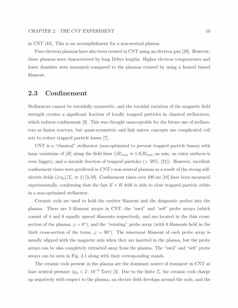
2.3 Confinement
Stellarators cannot be toroidally symmetric, and the toroidal variation of the magnetic field
strength creates a significant fraction of locally trapped particles in classical stellarators,
which reduces confinement [9]. This was thought unacceptable for the future use of stellara-
tors as fusion reactors, but quasi-symmetric and link mirror concepts use complicated coil
sets to reduce trapped particle losses [7].
CNT is a “classical” stellarator (non-optimized to prevent trapped particle losses) with
large variations of |B| along the field lines (|B|max ≈ 1.8|B|min on axis, on outer surfaces is
even bigger), and a sizeable fraction of trapped particles (> 50%, [21]). However, excellent
confinement times were predicted in CNT’s non-neutral plasmas as a result of the strong self-
electric fields (|eφp|/Te 1) [3,59]. Confinement times over 100 ms [10] have been measured
experimentally, confirming that the fast E × B drift is able to close trapped particle orbits
in a non-optimized stellarator.
Ceramic rods are used to hold the emitter filament and the diagnostic probes into the
plasma. There are 3 filament arrays in CNT: the “nw4” and “se8” probe arrays (which
consist of 4 and 8 equally spaced filaments respectively, and are located in the thin cross-
section of the plasma, ϕ = 0), and the “rotating” probe array (with 8 filaments held in the
thick cross-section of the torus, ϕ = 90). The innermost filament of each probe array is
usually aligned with the magnetic axis when they are inserted in the plasma, but the probe
arrays can be also completely extracted away from the plasma. The “nw4” and “se8” probe
arrays can be seen in Fig. 2.1 along with their corresponding stands.
The ceramic rods present in the plasma are the dominant source of transport in CNT at
base neutral pressure (pn < 2 · 10−8 Torr) [3]. Due to the finite Te the ceramic rods charge
up negatively with respect to the plasma, an electric field develops around the rods, and the

CHAPTER 2. THE CNT EXPERIMENT 11
resulting E ×B drift allows the electrons to leave the confining region.
A retractable emitter has been installed in CNT to study the confinement of plasmas
in the absence of ceramic rods [4]. The system is designed to extract the emitter from the
plasma faster than the confinement time. However, the measured confinement times after
retraction are shorter than in steady-state plasmas. P.W. Brenner’s thesis [11] describes the
efforts conducted to create and diagnose plasmas without internal ceramic rods, which will
be essential for the future operation of positron-electron plasmas in a stellarator.
The other major source of transport in pure electron plasmas is neutral-driven trans-
port, which is presumably caused by electron-neutral collisions, but is much higher than ex-
pected [3]. In order to understand this apparent inconsistency, the particle orbits in CNT’s
complicated 3D geometry were numerically simulated by B. Durand de Gevigney [21], show-
ing that the variation of the electric potential on magnetic surfaces leads to the existence of
open orbits for a large fraction of the electrons.
A conducting boundary was installed in CNT’s 64 tilt angle configuration in order to
set the electrostatic boundary condition at the plasma edge, thereby improving the match
between equipotential and magnetic surfaces. This was predicted to improve confinement by
making the electrons E×B drift within a magnetic surface (vE×B = (B×∇ψ)/B2 ∂φ/∂ψ),
thus reducing the cross-surface transport [21,45]. Although this did lead to improved confine-
ment, the improvement in neutral-driven transport with the conducting boundary installed
was less than expected, presumably because the boundary was significantly misaligned to
the magnetic surfaces [10].
Progress in the understanding and improvement of confinement in CNT is presented in
detail in P.W. Brenner’s thesis [11].
2.4 Equilibrium
Force balance and the fast temperature equilibration along the magnetic field lines determine
that the electrons are in a Boltzmann distribution function on each magnetic surface, ne =
N(ψ) exp (eφ/Te(ψ)) [59]. ψ is the magnetic flux enclosed by a magnetic surface, and is
commonly used as the magnetic surface coordinate [9] (on the magnetic axis of the surfaces,
ψ = 0; while ψ = 1 corresponds to the last closed magnetic surface).

CHAPTER 2. THE CNT EXPERIMENT 12
Equilibrium also has to satisfy Poisson’s equation. Therefore, the fundamental equation
describing the equilibrium of a pure electron plasma confined on magnetic surfaces is [59]:
∇2φ =e
ε0N(ψ) exp
(eφ
Te(ψ)
)(2.2)
This non-linear equation has been solved numerically [20,45,58], showing some interesting
features of CNT’s equilibrium. Publications by T.S. Pedersen [58] and R.G. LeFrancois [45]
investigate the benefits of having a conducting boundary conforming to the edge of the
plasma, and the effects of varying the number of Debye lengths in the plasma. The elec-
trostatic potential tends to be constant on surfaces where many Debye lengths are present
(〈a〉/λD > 10), but the potential varies significantly on magnetic surfaces for plasmas with
few Debye lengths (〈a〉/λD 1).
Another intrinsic characteristic of the equilibrium in CNT is the existence of large den-
sity variations along the magnetic field lines. A similar effect has been observed in Penning
traps [23], but the density variation in CNT is enhanced due to the large toroidal varia-
tion of the shape of the magnetic surfaces [44]. This large density variation was predicted
numerically by R.G. Lefrancois [44], and confirmed experimentally by M.S. Hahn [28].
2.5 Diagnostics
2.5.1 Equilibrium measurements
Basic equilibrium experiments involve measuring the plasma potential, temperature, and
density. Measurements of the radial profiles of these parameters are also done with simple
10 W tungsten filaments, working as emissive (hot) probes or Langmuir (cold) probes. The
probes are mounted on the same ceramic rods used to hold the emitter filament. The emitter
is usually aligned close to the magnetic axis to create the plasma, and the other filaments
are used to diagnose the plasma at different radial locations between the axis and the plasma
edge.

CHAPTER 2. THE CNT EXPERIMENT 13
Electron temperature and density
Te and ne are determined through the interpretation of Langmuir I-V characteristics [42],
which requires the simultaneous measurement of the current and voltage of a biased filament
probe. The potential is measured using a voltage divider, and the current from the voltage
drop across a resistor in series with the bias power supply and the probe.
In a pure electron plasma ne cannot be obtained from the ion saturation current, as it is
usually done in quasi-neutral plasmas [34]. However, ne and Te can still be determined from
the Langmuir I-V characteristics. If the electrons are in a Maxwellian distribution, the I-V
characteristics will present an exponential region, which becomes linear in a semi-logarithmic
plot log (Iprobe) vs Vprobe−φplasma. This linear region has a slope proportional to 1/Te, and a
y-intercept given by ln(14eneveA
)[42], where ve is the average thermal speed of the electrons,
and A is the area of the probe. Hence, Te is obtained from the slope of a fit in the linear
region, and ne from the y-intercept. This method exponentially amplifies uncertainties in
the y-intercept of the fit, which results in error bars in ne of one order of magnitude in some
cases. This measurement procedure was first developed by J.P. Kremer [42], then further
refined by J.W. Berkery and M.S. Hahn, and is also extended in my thesis.
Plasma potential
The plasma potential was measured in this thesis using two different methods: the deviation
potential [42] and the emissive probe floating potential [29]. The deviation potential method
studies the hot (emissive) and cold (non-emissive) I-V characteristics of the same filament
probe and determines the plasma potential as the potential at which the hot characteristic
deviates from the cold curve (i.e., the hot probe becomes slightly more negative than the
local plasma potential and begins to emit electrons). The emissive probe floating potential
method measures the voltage required to float a hot emissive filament inserted in the plasma.
The deviation potential method is generally more precise, but requires voltage sweeps over
long time scales, and only steady-state values of the potential can be measured. A more
detailed description of both procedures can be found in [29, 42] and also in Section 3.3.1 of
this thesis.
The fluctuations in the plasma potential described in Chapters 4 and 5 were detected by

CHAPTER 2. THE CNT EXPERIMENT 14
measuring the oscillating current in an internal emissive filament floated by having a capaci-
tor to ground. The amplitude of the oscillations is given by the fluctuations of the potential
in the plasma (converted from measurements of the current by using the I-V characteristic
of the emissive filament). The floating emissive probe was attached electrically to a simple
op-amp current to voltage converter circuit.
2.5.2 Spatial structure of the oscillations
Capacitive probes
A new set of capacitive probes3 was designed and constructed for this thesis to study the
toroidal and poloidal structure of the oscillations observed in the 78 tilt angle configuration.
This method requires the use of a limiter to effectively measure the oscillations of the image
charge in the probes. The limiter was installed at the thick poloidal cross-section of the torus
scraping off the plasma at ψ > 0.8, and thus ensuring that the electrons leaving the plasma
are not collected by the capacitive probes. Nevertheless, capacitive probes were successfully
used in CNT’s 64 configuration without a limiter installed in order to measure the poloidal
structure of the ion-driven instability [50]. In that case, the capacitive probe misaligned
furthest acted like a limiter collecting all of the electrons in the intersected magnetic surface.
Each capacitive probe was made of a copper disc of 5 cm in diameter, and was installed
facing the plasma ∼ 2 cm away from the outermost magnetic surface. The probes were
arranged in two different arrays perpendicular to each other. One array was made up of 5
probes placed around the thick poloidal cross-section of the stellarator. The second array
consisted of 6 probes located along the toroidal angle. Fig. 2.2 shows the location of both
probe arrays in a toroidal and a poloidal cross-section of the torus. The copper discs and the
limiter were held by aluminium rods (0.45 cm in diameter), and ceramic washers were used
to ensure that the probes were electrically isolated from the grounded aluminum structure.
The assembly of the image charge probes and the limiter was installed in the spot normally
used for the rotating probe. Although the two arrays consist of a discrete number of probes,
they provide enough spatial resolution to determine the poloidal and toroidal mode numbers,
3I designed the set of capacitive probes and supervised its construction by the undergraduate students
Derek Hernandez, Ignacio Garcıa-Cruzado, and Daniel Cosson.

CHAPTER 2. THE CNT EXPERIMENT 15
Figure 2.2: Left and center: Layout of the capacitive probe arrays in a toroidal cross-section,
and around the thick poloidal cross-section of the torus (the dashed line is a projection of
the magnetic axis). Rigth: The capacitive probes installed in the stellarator. ψ = 0.8 surface
glowing in order to align the limiter and the probes.
and the direction of propagation of the mode by measuring the phase delay of the oscillations
detected in the different probes.
Conducting boundary
The conducting boundary installed in CNT’s 64 configuration consisted of 13 copper meshes
electrically isolated from each other, so the different sectors could be also used as capacitive
probes to characterize the structure of the modes. The conducting boundary was significantly
misaligned (the meshes cut off ψ > 0.63 surfaces), and a limiter probe (initially installed
to use the copper meshes as capacitive probes) was removed for the experiments conducted
during this thesis, because it reduced the plasma volume even further.
The layout of the copper sectors was designed to provide some spatial resolution to mea-
sure the toroidal and poloidal structure of the modes. However, the spatial resolution of
conducting boundary was quite limited (e.g., there were only 4 meshes covering the toroidal
angle) and this resulted in significant spatial aliasing. For this reason, the measurements of

CHAPTER 2. THE CNT EXPERIMENT 16
Table 2.1: Location of the capacitive probes. See layout of the probes in Fig. 2.2
Toroidal array
Probe ϕ angle wrt probe T1
T2 31
TP3 44
T4 63
T5 83
T6 105
Poloidal array
Probe θ angle wrt probe P1
P2 26
TP3 60
P4 103
P5 124
the mode structure obtained with the conducting boundary were not conclusive by them-
selves. The spatial structure of the modes described in this thesis was studied by using the
set of capacitive probes described in the previous subsection and a high speed camera.
Fast camera
Since CNT’s plasmas emit sufficient light in the visible range for pn > 10−5 Torr [12],
the characteristic low frequency oscillations of our quasi-neutral plasmas (Chapter 5) have
been successfully observed for the first time in this thesis with a Vision Research Phantom
v7.1 camera 4. This is a high speed SR-CMOS 8-bit monochrome camera. Movies at full
resolution (800× 600 pixels) can be taken at 4,800 fps (frames per seconds), but the camera
can also record at sampling frequencies up to 160,000 fps at reduced resolution (limited by
the maximum amount of data that the camera can handle per second). For this thesis, movies
were typically captured at sampling frequencies between 40,000 and 75,000 fps, providing
enough spatial and temporal resolution for the characterization of the mode. Higher frame
rates yield unacceptable signal-to-noise ratios in CNT (less light is captured per frame as
the sampling frequency is increased).
The plasma was recorded from two different observation ports in the vacuum chamber
(Fig. 2.3): the “nw” side window (which looks radially into the plasma), and the top view
window (looking perpendicularly at the thick poloidal cross section of the plasma). The fast
4The High Speed Camera was borrowed from the CTX experiment.

CHAPTER 2. THE CNT EXPERIMENT 17
Figure 2.3: Representation of the view ports of the chamber used to record the plasma with
the High Speed Camera: “nw” side port, and the top view port.
imaging experiments also made use of a floating emissive filament in order to correlate the
density oscillations observed in the camera with the fluctuations of the plasma potential,
and also use the signal in the electrostatic probe as the time reference to compare movies
taken from different view ports.
2.5.3 Data acquisition
The different electronic circuits used to measure φplasma, Te, ne, the emission current, or the
oscillations in the image charge provide an analog output between -10 and +10 V propor-
tional to the plasma parameter of interest. These signals are collected by a 12 bit digitizer 5
operated at a maximum sampling frequency of 1.25/n MHz per channel (where n is the
number of channels used in each card). In my experiments one card was usually sampling at
low frequencies (typically 1-10 kHz per channel) to measure steady state parameters of the
plasma (e.g., emitter bias voltage or emission current), while the other cards measured the
oscillations in the plasma potential and higher sampling frequencies were required (some-
times only one channel had to be used per card to provide the maximum Nyquist frequency
5National Instruments PXI-6071E cards

CHAPTER 2. THE CNT EXPERIMENT 18
available, 625 kHz). Signals recorded at high sampling frequencies were always filtered at
the Nyquist frequency to avoid artifacts.
2.6 Relevant frequencies of CNT’s plasmas
Most of my research concerns the characterization of oscillations in plasmas of arbitrary
neutrality. In order to identify the physics involved in these oscillations it is essential to
estimate the relevant frequencies in CNT and study its dependence on experimentally ad-
justable parameters (such as the magnetic field strength). Some important frequencies and
timescales of our plasmas are briefly described below and summarized in Fig. 2.4:
1. Electron parallel equilibration timescale. The parallel equilibration timescale of
electrons in magnetic surfaces (τ‖) can be estimated as the time a thermal electron
needs to travel toroidally and poloidally around a magnetic surface.
τ‖ ≈ 2πR
ιvth(2.3)
where R is the major radius of the plasma, ι is the rotational transform, and vth is
the electron thermal velocity (vth =√
2Te/me). For a typical 4 eV plasma, τ‖ ≈ 6µs.
Therefore, a plasma in equilibrium is expected to damp all frequencies below 150 kHz
through parallel force balance.
2. E×B rotation frequency. Non-neutral plasmas present fast E×B drifts, due to their
strong self E fields. In order to have an equilibrium, the plasma has to equilibrate on
a magnetic surface through parallel dynamics faster than the E×B drift. Otherwise,
a diocotron type instability [39] is likely to occur. The E×B rotation frequency is:
fE×B =E/B
2π〈a〉 (2.4)
where 〈a〉 is the minor radius of the plasma. CNT usually operates at magnetic field
strengths between 0.02 and 0.1 T and the potential drop across the plasma is 50 V
(when the 0 V boundary condition is set at the coils and the chamber) to 200 V (with a
conducting boundary installed at the edge of the plasma). Thus, fE×B typically ranges
between 5 and 70 kHz.

CHAPTER 2. THE CNT EXPERIMENT 19
3. Ion bounce frequency. Heavy ions (such as N+2 ) are largely unmagnetized in CNT
(Fig. 3.14) and they follow complicated trajectories in the plasma. As heavy ions are
drawn into the electron rich plasma, a large fraction of the potential drop in the plasma
is transferred to their parallel velocity, and they bounce from one side of the electron
plasma to another. In Penning traps the ion motion is analytically solvable [19], but
in CNT ions do not present a simple well defined poloidal rotation frequency. Mark-
steiner’s thesis [49] studied the distribution of the ion bounce frequencies in CNT,
showing that essentially all N+2 ions at 0.02 T bounce between 14 and 83 kHz, with 25
kHz being the dominant bounce frequency.
4. Cyclotron frequency. A charged particle moving perpendicularly to the direction of
a uniform magnetic field performs a circular motion at the cyclotron frequency. The
cyclotron frequency is defined as:
fc =qB
2πm(2.5)
Fig. 2.4 includes the electron cyclotron frequency and the cyclotron frequencies of the
most commonly used ions in CNT.
5. Plasma frequency. The plasma (or Langmuir) frequency is defined as:
fp =1
2π
√e2ne
ε0me
(2.6)
The use of electrostatic Langmuir waves has been proposed to measure the electron
density in CNT [29,41], but so far attempts to use this method have been unsuccessful,
probably because of the poor RF coupling between the function generator and the
antenna.
For a pure electron -200 V plasma, ne ≈ 1012 m−3, while the density of CNT’s quasineu-
tral plasmas is ne ≈ 1015 m−3. Therefore, fp ranges from 9 to 290 MHz.

CHAPTER 2. THE CNT EXPERIMENT 20
Figure 2.4: Relevant frequencies in typical CNT plasmas (φe = −200 V, 0.02 ≤ B ≤ 0.1 T).

Chapter 3
Plasmas of Arbitrary Neutrality
Even at CNT’s base pressure (pn ≤ 2 · 10−8 Torr), neutrals are ionized in the vacuum
chamber (preferentially at locations of high Te, near the outer magnetic surfaces) and ions
are drawn into the electron rich plasma, which would cause the neutralization of the plasma
in ∼ 0.5 s in the absence of an ion loss mechanism [2]. However, the ceramic rods inserted
in the plasma act as steady state sinks for ions. The rods are charged up negatively with
respect to the plasma (due to the finite Te) and ions become neutralized when they collide
with the rods. The ion content in our plasmas can be controlled by adjusting the neutral
pressure in the chamber, thus varying the steady state balance between the ionization of
neutrals and the recombination at the rods. At pn = 2 · 10−8 Torr, the ion fraction (fi =
ni/ne) is calculated to be fi < 1% [2]. CNT’s pure electron plasmas are macroscopically
stable [43], but the accumulation of ions affects the equilibrium and changes the properties
of the plasma radically. This section describes how the plasma potential, ion gyro-radius,
electron temperature, and dielectric constant evolve with the degree of neutralization of
the plasma. An overview on the spontaneous oscillations detected in plasmas of arbitrary
neutrality is given in Section 3.6. Chapters 4 and 5 describe in detail the oscillations observed
in partially neutralized (10−4 < η < 1) and quasi-neutral plasmas (η < 10−4) respectively.
Unless otherwise specifically stated, the experimental results shown in this Chapter refer
to the 64 tilt angle configuration with the conducting boundary installed.
21

CHAPTER 3. PLASMAS OF ARBITRARY NEUTRALITY 22
3.1 Presence of ions in CNT
A 7.4 cm2 copper plate was inserted at ψ ≈ 0.4 in the ϕ = 90 cross section of the torus in
order to measure the ion density, and explore the role of the magnetic field strength, emitter
bias, and neutral pressure. The ion density was determined through the interpretation of
Langmuir I-V characteristics. Since the probe sheath expands as the probe is biased more
negatively [34], the collected ion current increases with the probe potential, and Isat was
determined as the current at which φprobe − φplasma = −100V from a linear fit of the ion
saturation region. Ions in CNT are only weakly magnetized and are predicted to have kinetic
energies that are a large fraction of the potential drop across the plasma, so the ion saturation
current scales like Eq. 3.1:
Isat ≈ eAprobeni
√eφp + 3Te
8mi(3.1)
This estimate was used to compute the ion content (ni), instead of the Bohm sheath criterion.
For electron-rich non-neutral plasmas (|eφp| Te), Eq. 3.1 gives the ions a higher arrival
rate than the Bohm criterion, while for CNT’s quasineutral plasmas (|eφp| Te) the ion
velocity is essentially determined by the electron temperature, which is consistent with the
Bohm criterion.
Both neutral pressure and emitter bias voltage are predicted to increase the ion content
of the plasma since the ionization frequency scales linearly with the neutral number density,
and the electron density and temperature increase with the emitter bias, causing the rate of
ionization of neutrals to grow. Experimental results confirm the linear dependence of the ion
density on neutral pressure and show a rapid increase of the ion fraction with the emitter
bias (Fig. 3.1).
Although the magnetic field strength may reduce the transport rate, it does not affect the
equilibrium in CNT directly and no clear relationship was found experimentally between ne
and B [41]. Numerical simulations [49] predict that the ion fraction can be 3.7 times higher
at B = 0.1 T than at 0.02 T for plasmas with a non-negligible fraction of H+2 . However, the
effects of the magnetic field strength on the ion content are not totally understood based
on the experimental results. The measured ion saturation current usually decreases slightly
with the magnetic field strength, but this can be caused by an indirect effect of the measuring
procedure. At higher B fields, ions become somewhat magnetized and their orbits may be

CHAPTER 3. PLASMAS OF ARBITRARY NEUTRALITY 23
Figure 3.1: Ion content in CNT as a function of the neutral pressure for three different
emitter biases (N+2 − e− plasmas at B = 0.08 T).
sufficiently affected that the probe cannot collect ions from all directions, thus reducing the
ion saturation current.
For B ≥ 0.06T and φe ≥ −100V, the ion content saturates for neutral pressures above
4 · 10−6 Torr (Fig. 3.1). This observation may be a further proof that our plasmas become
quasi-neutral at high neutral pressures. The saturation of the ion content at high neutral
pressures is also expected for the most negative emitter bias (-200 V). However, the power
supplies used for these experiments cannot handle ion saturation currents above 100µA
(which corresponds to ni ≈ 1.5 · 1014m−3), and also when values of the measured current
approach this technical limit, it becomes harder to interpret the Langmuir I-V characteristics
(no linear slope associated to the ion saturation current is observed in the I-V curves). This
is the reason why the ion content at φe = −200V could not be measured above 2 · 10−6
Torr in Fig. 3.1. At the highest neutral pressures (pn ≥ 10−5 Torr) the emission current is
a strong function of the temperature of the emitter filament, and the slight drop of the ion
density at the lower bias voltages is believed to be related with a small fall in the power
supplied by the batteries used to heat the emitter filament.

CHAPTER 3. PLASMAS OF ARBITRARY NEUTRALITY 24
Ion probes of the same dimensions and characteristics were aligned parallel and perpen-
dicularly to the magnetic field lines (minimizing for each orientation the fraction of magnetic
surfaces intersected by the probe). It was observed that the measured ion saturation current
is not dependent on the orientation of the probe relative to the field lines, which is typical
for plasmas where the ions are weakly magnetized.
3.2 Degree of non-neutralization (η)
In order to obtain more meaningful interpretations of the behavior of the relevant parameters
under study in partially neutralized plasmas, it is convenient to define the degree of non-
neutralization of the plasma (η) as the difference between the electron and the ion density
divided by the total density of charged particles in the plasma (Eq. 3.2):
η ≡∣∣∣∣ne − Zni
ne + Zni
∣∣∣∣ (3.2)
Fig. 3.2 shows how CNT can vary continuously η from 1 (pure electron plasmas, essen-
tially reached at base pressures) to 1 (quasi-neutral plasmas) by adjusting the neutral
pressure in the chamber, thus varying the steady state balance between the ionization of
neutrals and the recombination at the rods. CNT is not only able to vary continuously η,
but also to operate steadily at any given value of η shown in Fig. 3.2. Penning-Malmberg
traps and pure toroidal cannot confine partly neutralized or quasi-neutral plasmas, and op-
erate close to η = 1. Table 3.1 provides an estimation of η for other representative plasmas,
showing that CNT can operate in a range of η values that expand 5 orders of magnitude,
while other quasi-neutral experiments present very limited flexibility to vary η significantly,
but typically operate at degrees of non-neutralization 3 orders of magnitude lower. The esti-
mates of η for quasi-neutral experiments in Table 3.1 assumed |eφ| ≈ Te, which is generally
true in quasi-neutral plasmas to satisfy ambipolarity.
η cannot be accurately determined using the experimentally measured values of ne and
ni only. The measurements of ne in CNT are affected by large uncertainties (almost one
order of magnitude in some cases); the I-V characteristics used to determine ne are rather
noisy in partially neutralized plasmas [42], and the probe bias power supplies cannot handle
the currents involved in measurements above 10−6 Torr (ne 1014 m−3).

CHAPTER 3. PLASMAS OF ARBITRARY NEUTRALITY 25
Figure 3.2: Degree of non-neutralization (η) as a function of the neutral pressure in the
chamber for different emitter bias voltages (N+2 − e− plasmas at 0.02 T).
Table 3.1: Estimation of η for other representative plasmas
ne (m−3) Te (eV) minor radius (m) η
Penning-Malmberg trap [48] 1012 - 1013 1 0.015 1
LNT-II pure toroidal trap [76] 5 · 1012 1 - 100 0.05 1
CNT 1012 - 1016 4 - 60 0.15 10−5 − 1
JT60 [36] 3 · 1019 104 0.89 5 · 10−8
HBT-EP [52, 72] 1019 70 0.15 3 · 10−8
DIII-D [68] 1020 5 · 103 0.7 10−8
ITER [31, 73] 1020 5.3 · 103 2 1.5 · 10−9

CHAPTER 3. PLASMAS OF ARBITRARY NEUTRALITY 26
In this thesis η is determined with good accuracy using Poisson’s equation, and assuming
CNT plasma has a cylindrical geometry of radius r = 0.15 m. From Poisson’s equation in a
cylinder:
1
r
∂
∂r
(r∂ϕ
∂r
)= − σ
ε0
ϕ(r) = − σ
4ε0r2 + ϕ(0) (3.3)
where, σ = qini − ene, the electron and ion density profiles are assumed to be flat, ni
is measured from the ion saturation current in a copper probe (affected by smaller error
bars than ne), the plasma is grounded at the edge (ϕ(r = 0.15) = 0V), and ϕ(0) is taken
from the measurements of the plasma potential very close to the magnetic axis (ψ ≈ 0.1, see
Section 3.3), which is typically known within ±1 V.
Therefore, the electron density can be calculated as:
ne = ni − 4ε0er2
ϕ(0) (3.4)
And the determination of η is trivial using Eq. 3.2:
η =
∣∣∣∣ −4ε0er2ϕ(0)
2ni − 4ε0er2ϕ(0)
∣∣∣∣ (3.5)
In order to check the validity of the method, the electron density was calculated using
Eq. 3.4 and compared with the experimental measurements of ne obtained interpreting the
I-V characteristic of a cold filament [42]. Fig. 3.3 shows that the estimated values of ne
in the cylindrical plasma are in good agreement with the experimental measurements. For
pressures below 2 · 10−7 Torr, the estimation of ne in a cylinder is within the error bars of
the experimental results, and for higher pressures, the value obtained from Eq. 3.4 seems to
be a reasonably good estimate. At base neutral pressures (pn ≤ 2 · 10−8 Torr), the estimate
obtained from Poisson’s equation can also be compared with numerical reconstructions of the
equilibrium in CNT [20], finding also good agreement between the approximate expression of
Eq. 3.4 in a cylinder, and the numerical reconstructions in CNT’s complicated 3D geometry.
There are two factors that account for the rapid drop of η when the neutral pressure
is increased (Fig. 3.2). Most importantly, as ni increases, the number of electrons grows
accordingly trying to maintain the voltage drop across the plasma, and the term 4ε0er2ϕ(0)

CHAPTER 3. PLASMAS OF ARBITRARY NEUTRALITY 27
Figure 3.3: Comparison of the measured electron density with the estimation of ne assuming
a cylindrical geometry (Eq. 3.4). N+2 − e− plasmas, B = 0.02 T, φe = -200 V.
matters less. But also when the plasma decouples from the emitter bias (see Section 3.3),
the term 4ε0er2ϕ(0) becomes smaller, specially for pn > 2 · 10−6 Torr (see Fig. 3.4).
3.3 Plasma potential
One of the clearest consequences of the accumulation of ions in CNT is the decoupling of the
potential profiles from the emitter bias voltage. In pure electron plasmas the emitter bias
voltage dictates the plasma potential. Even when the degree of non-neutralization decreases
from η ≈ 1 to 0.1, the ion content grows, but the electron density increases accordingly to
maintain the voltage drop across the plasma (Fig. 3.5). However, for η < 0.1 the plasma
potential (φp) begins to decouple from the emitter bias (φe). Pure electron plasmas in CNT
are characterized by strong negative electric fields imposed by the emitter bias, but as our
plasmas approach quasineutrality the electrostatic potential is much more modest, since it
comes close to that which would be set by ambipolarity as the injection of electrons matters
less for the radial fluxes of charge.

CHAPTER 3. PLASMAS OF ARBITRARY NEUTRALITY 28
Figure 3.4: Evolution of the different terms in Eq. 3.4 as a function of neutral pressure
(N+2 − e− plasmas, B = 0.02 T, φe = -200 V).
Figure 3.5: Evolution of the plasma potential at ψ ≈ 0.1 while emitting electrons on the
magnetic axis at -200 V (N+2 − e− plasmas, B = 0.02 T).

CHAPTER 3. PLASMAS OF ARBITRARY NEUTRALITY 29
3.3.1 Methods for the measurement of φp
Two methods have been used in order to determine the plasma potential: the deviation
potential [42] and the emissive probe floating potential [29]. The deviation potential method
compares the hot (emissive) and cold (non-emissive) I-V characteristics of the same probe.
The probe used is a halogen filament, which can only collect charged particles when cold,
but can emit electrons by thermionic emission when the filament is heated. The plasma
potential is determined as the potential at which the hot probe is slightly more negative
than the plasma potential, and starts to emit electrons (the hot I-V characteristic deviates
from the cold curve). The emissive probe floating potential method measures the voltage
required to float a hot emissive filament. For this purpose, a current source is used to bias
the heated filament at the voltage where the current is set to emit a few nA, thus the hot
filament is reasonably close to floating. Having a source emitting a few nA only affects
marginally our plasmas at base neutral pressures, where the emission currents are of the
order of a few µA.
For η > 0.1, the deviation potential method is more accurate, but as the ion content
increases, the plasma becomes hotter, and the characteristic of the hot filament becomes less
sharp resulting in less accurate measurements. Also, the deviation potential requires voltage
sweeps over a long time and the power supplies used to bias the probes cannot handle the
currents involved in the measurements where η < 0.01. The emissive probe floating potential
method introduces a systematic error in the measurements (φfloat = φp − αTe/e, where
α ≤ 1 [80]), but the method is robust in the entire range of pressures explored experimentally
and measurements are in good agreement with the deviation potential results where it is
possible to use both methods.
3.3.2 Parameter dependence
A series of experiments were conducted to study systematically the dependence of the plasma
potential on the degree of non-neutralization, emitter bias voltage, magnetic field strength,
ion species, and magnetic configuration. For the experiments described in this Section, the
potential was measured using a heated emissive filament placed at ψ ≈ 0.15 (spot 2 of the
nw4 probe array) and floated by using the current source circuit.

CHAPTER 3. PLASMAS OF ARBITRARY NEUTRALITY 30
Figure 3.6: φp/φe at ψ ≈ 0.15 as the neutral pressure is increased for different emitter bias
voltages (N+2 − e− plasmas at 0.06 T).
Effect of the emitter bias and the ion content
Basic observations show that the plasma potential decouples rather abruptly from the emitter
bias at a certain neutral pressure threshold. This threshold is a function of the emitter bias,
at lower emitter biases the plasma decouples from the emitter at higher pressures (Fig. 3.6).
Even the potential profiles do not detach from the emitter in a φe = −50 V plasma at
B ≥ 0.04 T for the range of pressures explored in the experiments (pn ≤ 5 · 10−5 Torr). This
suggests that the ion content may be responsible of the separation of the plasma potential
profiles from the emitter (more negative emitter bias voltages are associated with higher
electron densities, and thus higher ionization rates).
Analyzing the plasma potential as a function of the ion content in our plasma, it can be
seen that the potential of the floating emissive probe drops below 50% of the emitter bias
when the ion content exceeds a threshold between 5 · 1013 and 1014 m−3 (Fig. 3.7). In the
experiments performed with -50 V plasmas, the ion content only reaches 5 · 1013 m−3 at the
lowest B field explored (B = 0.02 T) and therefore the potential in the floating emissive
probe always remains close to the emitter bias (0.7 < φp/φe < 1) for B ≥ 0.04 T.

CHAPTER 3. PLASMAS OF ARBITRARY NEUTRALITY 31
Figure 3.7: φp/φe at ψ ≈ 0.15 as a function of the ion content in the plasma (N+2 − e−
plasmas at 0.06 T).
However, the abrupt decoupling of the plasma potential from the emitter bias voltage
coincides with the onset of the saturation of the emission current (see Fig. 3.17), suggesting
that the decoupling might be related to the emission limit of the filament used to create the
plasma. The emitter filaments used in CNT are rated for 6 V, but 4 V batteries produce
enough heating to emit electrons and are normally used to produce our plasmas. The emis-
sion limit depends on the temperature of the emitter filament, which in turn, is a function
of the current supplied by the heating battery. Fig. 3.8 shows the emission current limit of
CNT’s filaments when a 4 V and a 6 V battery are used for heating. In order to eliminate
the effect of the plasma in the investigation of the emission limit, no B field was generated by
the coils during these experiments, which prevented the formation of plasma. For φe = −200V (which is a usual operating point in our experiments), a filament heated by a 6 V battery
can emit 4 times more current than when a 4 V battery is used.
Therefore, in order to clarify whether the separation of the plasma potential from the
emitter is caused by an emission limit or occurs when a threshold ion content is exceeded, a set
of experiments was conducted to study how the decoupling threshold depends on the emitter

CHAPTER 3. PLASMAS OF ARBITRARY NEUTRALITY 32
Figure 3.8: Emission current limit of the filament used to create the plasma as function of
the filament bias voltage and for two different heating batteries (4 and 6 V). The filament
did not create a plasma during these experiments.
filament temperature and the presence of an additional ceramic rod in the plasma. Although
the emitter filament is able to emit significantly higher currents when a 6 V battery is used
for heating, Fig. 3.9 shows that the decoupling of the plasma potential occurs essentially at
the same neutral pressure when either a 4 V or a 6 V battery is used, implying that the
mechanism of the plasma potential detachment is not related to the emission limit. When
an additional rod is inserted in the thin cross section of the plasma, the ion density at a
given neutral pressure is halved everywhere [49]. The neutral pressure scan performed with
a second ceramic rod inserted in the plasma shows that the pressure threshold where the
plasma potential drops below 50% of the emitter bias occurs at approximately two times
higher pressure (Fig. 3.9), which essentially corresponds to the same ion content threshold
as when a single rod is present. This provides strong evidence to conclude that the ion
content is responsible of the decoupling of the plasma potential from the emitter bias.

CHAPTER 3. PLASMAS OF ARBITRARY NEUTRALITY 33
Figure 3.9: φp/φe as function of pn, evaluating the effect of different filament temperatures
(4 and 6 V heating batteries) and the presence of an additional ceramic rod in the plasma
(N+2 − e− plasmas at 0.04 T).
Effect of the magnetic field strength
The role of the magnetic field strength on the threshold required for the plasma potential
to decouple remains unclear. For low emitter bias voltages (|φe| ≤ 100 V), plasmas with
more magnetized ions detach from the emitter bias at higher neutral pressures (Fig. 3.10).
However, for |φe| ≥ 150 V the pressure threshold of the potential decoupling is independent
of the magnetic field strength.
When the plasma is completely decoupled from the emitter (0 < φp/φe < 0.1), |φp| in-creases with the magnetic field strength (charge is confined better at higher B field strengths),
and typically higher |φe| are associated to slightly lower measured values of |φp| (becauseplasmas created by more negative emitter bias voltages present higher ion contents). When
the plasma potential is dictated by the emitter (0.8 < φp/φe < 1), |φp| is somewhat smaller
for higher magnetic field strengths.

CHAPTER 3. PLASMAS OF ARBITRARY NEUTRALITY 34
Figure 3.10: Evolution of φp/φe at ψ ≈ 0.15 while emitting electrons on axis at -100 V
(background pressure of N2).
Effect of different ions species
The behavior of the potential in a floating emissive probe inserted in plasmas with different
ion masses (Ar+ − e− and He+ − e− plasmas) is very similar to the results described so far
for N+2 − e− plasmas (Figs. 3.6 to 3.10). The ionization energies for Ar and N2 are very
similar (15.76 eV for Ar, and 14.53 eV for N) and Fig. 3.11 shows that the plasma potential
detaches from the emitter at essentially the same pressure (slightly lower for the case of Ar).
He has a much higher ionization energy (24.59 eV) and the plasma potential decouples from
the emitter bias at one order of magnitude higher pressures (∼ 10−5 Torr).
Effect of the magnetic configuration
The behavior of the plasma potential is almost identical in the 78 and the 64 configurations.
However, at high magnetic fields strengths (B ≥ 0.06 T) and degrees of neutralization close
to quasi-neutrality (4 · 10−6 < pn < 2 · 10−5 Torr), the measured floating emissive potential
is more negative for the 78 tilt angle (Fig. 3.12).
The dependence of the floating emissive potential on the emitter bias voltage and the

CHAPTER 3. PLASMAS OF ARBITRARY NEUTRALITY 35
Figure 3.11: φp/φe vs. neutral pressure for Ar+ − e−, He+ − e− and N+2 − e− plasmas
(φe = −200 V, B = 0.04 T).
magnetic field strength is very similar for both tilt angles. Partially neutralized plasmas
(pn < 10−6 Torr) present potentials very close to the emitter bias for both configurations and
all the magnetic field strengths and emitter voltages explored (0.02 ≤ B ≤ 0.1 T, and−400 ≤φe ≤ −100 V). Partially neutralized plasmas in the 78 configuration exhibit potentials
somewhat closer to the emitter bias (φp/φe > 0.80 for the 78 configuration, while φp/φe >
0.73 for the 64 configuration). Quasineutral plasmas present plasma potentials slightly more
negative in the 78 tilt angle. The behavior of the plasma potential in quasineutral plasmas
is essentially the same in both configurations: |φp| increases with the magnetic field strength
(Fig. 3.13), and more negative emitter biases are associated to higher ion content, and thus
the ratio φp/φe gets closer to ∼ 0.
3.4 Ion gyro-radius and electron temperature.
As the plasma potential (φp) decouples from the emitter bias (φe), the emitted electrons are
accelerated (φ = φe−φp) and, since CNT is essentially a collisionless plasma, the electrons

CHAPTER 3. PLASMAS OF ARBITRARY NEUTRALITY 36
Figure 3.12: φp/φe vs. neutral pressure for the two stellarator configurations studied so far:
64 and 78 tilt angle (electron-rich N+2 plasmas, φe = −200 V, 0.02 and 0.08 T).
Figure 3.13: Comparison of the dependence of the plasma potential on the magnetic field
strength for the 64 and the 78 tilt angle (N+2 − e− quasineutral plasmas, 2.5 · 10−5 and
4.0 · 10−5 Torr, φe = −200 V).

CHAPTER 3. PLASMAS OF ARBITRARY NEUTRALITY 37
become hotter (Fig. 3.14). The limitations with the power supplies described earlier in this
chapter prevented us from measuring Te for η < 10−2 in this set of experiments.
Ions, however, exhibit the opposite behavior. Part of the potential drop across the plasma
is transferred to the ions’ kinetic energy as they are drawn into the electron-rich plasma.
The ion motion is analytically solvable in a simple cylindrical plasma confined by an axial
magnetic field. The ion fluid rotates as a rigid body at a frequency ωi given by [18]:
ωi = −12ωci
[1−
(1 +
4ωE×B
ωci
)1/2]
(3.6)
where ωci is the ion cyclotron frequency, ωci = qB/mi, and ωE×B is the equilibrium E × Brotation frequency of the plasma. In the presence of strong magnetic fields and for light
ion species, ωi approaches ωE×B, thus as the plasma detaches from the emitter bias (the
potential drop across the plasma becomes smaller), the ions get colder. Fig. 3.14 assumes
the average perpendicular velocity of the ions in CNT is the E ×B velocity, and shows how
the ion gyro-radius (rLi = mivE×B/qB) normalized wrt the average minor radius of the torus
(〈a〉 = 0.15 m) evolves with η for a typical operating point of our experiments (B = 0.02 T).
When η ≈ 1 the ion gyro-radius is substantially bigger than the minor radius of the plasma,
rLi 〈a〉 (ions are highly unmagnetized), but quasi-neutral plasmas (η ≈ 0) present ion
gyro-radii of a few centimeters (rLi < 〈a〉).
3.5 Perpendicular dielectric constant
In CNT’s partially neutralized plasmas the measured frequency of the electric field oscilla-
tions (ω) is comparable to the ion gyro-frequency (ωci), therefore the perpendicular dielectric
constant (ε⊥) has to be evaluated as [27]:
ε⊥ = 1 +q2ni
ε0mi(ω2ci − ω2)
(3.7)
At low B field strengths (B ≤ 0.04) partially neutralized plasmas present oscillations
such that ω > ωci (see Fig. 2.4 and Chapter 4), hence ε⊥ is negative, and incident waves will
not penetrate deep into these plasmas. Fig. 3.15 evaluates ε⊥ for B ≤ 0.04 T taking ω as the
measured frequency of the ion resonant mode characterized in Section 4.2. For B ≥ 0.06 T

CHAPTER 3. PLASMAS OF ARBITRARY NEUTRALITY 38
Figure 3.14: Measured electron temperature compared to the normalized ion gyro-radius as
a function of the degree of non-neutralization (N+2 − e− plasmas at φe = −200 V and B =
0.02 T).
ε⊥ is always positive and grows more that 3 orders of magnitude as the plasma evolves from
pure electron (ε⊥ ≈ 1) to quasineutral (ε⊥ ≈ 2 · 103, Fig. 3.16). In Fig. 3.16 (B = 0.06 T)
we can also see that the electric field oscillations hit the resonance ω ≈ ωci at η ≈ 0.1. Since
ωci grows with the B field strength and the measured frequency of the E field oscillations
decreases slightly with B, this resonance is not observed at higher magnetic field strengths.
3.6 Oscillations in plasmas of arbitrary neutrality. Ba-
sic observations
One of the most relevant changes observed in partially neutralized plasmas in CNT is the
spontaneous appearance of unstable fluctuations when a certain ion content is exceeded.
Figs. 3.17 and 3.18 summarize the characteristics of the oscillations observed in partially
neutralized plasmas. Pure electron plasmas exhibit stable behavior: the charge loss rate
(emission current) scales linearly with the neutral pressure, and only oscillations with a very

CHAPTER 3. PLASMAS OF ARBITRARY NEUTRALITY 39
Figure 3.15: The perpendicular dielectric constant (ε⊥) presents negative values for B ≤ 0.04
T (N+2 − e− plasmas at φe = −200 V). The frequency of the electric field oscillations (ω) is
taken from the characterization of the ion-driven mode presented in Section 4.2.
Figure 3.16: Perpendicular dielectric constant (ε⊥) as a function of the degree of non-
neutrality of our plasma (N+2 − e− plasmas at φe = −200 V and B = 0.06 T).

CHAPTER 3. PLASMAS OF ARBITRARY NEUTRALITY 40
small signal-to-noise ratio are detected in a floating emissive probe inserted in the plasma.
The amplitude of the plasma oscillations starts increasing for η 0.1, and simultaneously the
loss rate of confined particles is enhanced, implying than the unstable fluctuations degrade
confinement. This was first reported by Q.R. Marksteiner [50], and was also observed in
this thesis (Fig. 3.17). A typical Fourier Spectrum of the detected oscillations is shown
in Fig. 3.18. When partially neutralized plasmas become robustly unstable, multimode
fluctuations are observed. The power spectrum broadens for η < 4 · 10−2 and is eventually
dominated by a ∼ 200 kHz mode. As the plasma accumulates more ions, the amplitude of
the oscillations grows steadily until a maximum is reached at η ≈ 3 · 10−3, coinciding with
the onset of the saturation of the charge loss rate. Partially neutralized plasmas with more
magnetized ions (either by raising the B field above 0.04 T or introducing light ions species,
such as He+) exhibit a single dominant mode (20 - 100 kHz) for degrees of non-neutralization
between η = 0.01 and 0.1. When the plasma approaches quasi-neutrality (η < 10−4) the
amplitude of the oscillations decreases, the spectrum narrows down, and finally the plasma
reverts to single mode behavior (1 - 20 kHz), even for weakly magnetized ions.
The electrostatic fluctuations in the plasma potential (φ) are detected by measuring the
oscillating current in an internal emissive filament which floats by virtue of having a capacitor
to ground. The amplitude of the detected oscillations is given by the fluctuations of the
potential in the plasma. The amplitude of the plasma potential oscillations is estimated
using the I-V characteristic of an emissive filament close to floating and the measured value
of the oscillating current shown in Fig. 3.17. The standard deviation of |eφ| normalized to
the measured Te is presented in Fig. 3.19, showing that the plasma is always subjected to
small oscillatory perturbations (|eφ|/Te < 1).
Since the current collected in an ion saturation probe (electrostatic probe strongly neg-
atively biased with respect to the plasma) is a reasonably good estimator of the plasma
density [34], a 9 cm2 ion probe was used to measure the oscillations in the plasma density
(n). The ion probe was biased 100 V more negatively than the local plasma potential, and the
current collected was measured through the voltage drop across 1 to 100 kΩ resistors using
a circuit identical to the one used to measure the emission current in our experiments [42].
Chapter 4 is devoted to the detailed characterization of the spontaneous oscillations
observed in electron-rich non-neutral plasmas (10−4 < η < 1). Chapter 5 describes the

CHAPTER 3. PLASMAS OF ARBITRARY NEUTRALITY 41
Figure 3.17: Evolution of the charge loss rate and the RMS of the oscillations in a floating
emissive probe as a function of the degree of non-neutralization (N+2 − e− plasmas, B = 0.02
T, φe = −200 V, 64 configuration).
parameter dependence and spatial structure of the mode detected in CNT’s quasi-neutral
plasmas (η < 10−4).
3.7 Summary
CNT can vary continuously the degree of neutralization of the plasma (η) from η = 1 (pure
electron plasmas) to η 1 (quasi-neutral plasmas) by adjusting the neutral pressure in
the chamber, which controls the volumetric ionization rate. CNT can also operate steadily
at any given value of η between 10−5 and 1, while other devices traditionally used for the
investigation of non-neutral and quasi-neutral plasmas present very limited flexibility to
change η significantly (Table 3.1).
As η evolves from pure electron to quasi-neutral, spontaneous fluctuations appear, and
the plasma potential decouples from the emitter. The insertion of an additional ceramic
rod in the plasma halves the total ion population at a given neutral pressure. It has been
observed that the neutral pressure threshold for both the development of fluctuations [49],

CHAPTER 3. PLASMAS OF ARBITRARY NEUTRALITY 42
Figure 3.18: Power spectrum of the signal on a floating emissive probe vs. degree of non-
neutralization. When partially neutralized plasmas become robustly unstable (η < 0.1),
multi-mode fluctuations are observed. (N+2 − e− plasmas, B = 0.02 T, φe = −200 V, 64
configuration).

CHAPTER 3. PLASMAS OF ARBITRARY NEUTRALITY 43
Figure 3.19: Standard deviation of |eφ| normalized to Te as a function of the degree of
non-neutralization (N+2 − e− plasmas, B = 0.02 T, φe = −200 V, 64 configuration).
and for the separation of the plasma potential (Section 3.3.2) is approximately doubled when
a second ceramic rod is present in the plasma, providing strong evidence that these changes
occur when a threshold ion content is exceeded.
In order to confirm that the decoupling of the plasma potential is not caused by an
emission limit of the filament creating the plasma, a set of experiments was also conducted
to study how the decoupling threshold was affected by the emitter filament temperature.
When 6 V batteries are used to heat the emitter, the filament can emit significantly higher
currents than with 4 V batteries. However, the separation of the plasma potential occurs
essentially at the same neutral pressure when either a 4 V or a 6 V battery is used (Fig. 3.9).
This chapter also evaluates how electron temperature, ion gyro-radius, and perpendicular
dielectric constant of the plasma change as η is varied 5 orders of magnitude. As a result
of the separation of φp from the emitter bias, the emitted electrons are accelerated, and
become hotter (Fig. 3.14). Ions, however, get colder as the plasma detaches from the emitter
bias. Since the average perpendicular velocity of the ions can be approximated as the E×Bvelocity at high magnetic fields and for light ion species (Section 3.4), the ion gyro-radius

CHAPTER 3. PLASMAS OF ARBITRARY NEUTRALITY 44
becomes smaller when the plasma decouples from the emitter bias (Fig. 3.14). In CNT, N+2
ions are essentially unmagnetized for η ≈ 1, but rLi is smaller than the minor radius of the
plasma for quasi-neutral plasmas.
Chapters 4 and 5 describe in detail the spontaneous oscillations observed in partially
neutralized (10−4 < η < 1) and quasi-neutral plasmas (η < 10−4) respectively.

Chapter 4
Oscillations in electron-rich
non-neutral plasmas
As the ion content increases in an electron-rich non-neutral plasma (1 > η > 10−4), the
plasma becomes unstable, and fluctuations are detected in electrostatic emissive probes
inserted in the plasma. This Chapter presents a description of the oscillations observed
in this regime, analyzing the dependence of the fluctuations on experimentally adjustable
parameters (magnetic field strength, plasma potential, degree of non-neutralization, different
ion species, and magnetic configuration), and the spatial structure of the detected modes.
Ions in CNT are typically largely unmagnetized (rLi 〈a〉 1), and exhibit a clear bounc-
ing motion as they are drawn into the electron-rich plasma [49]. Partially neutralized plasmas
with weakly magnetized ions develop multimode oscillations. However, more magnetized
ions travel closer to the E×B velocity and single mode oscillations are detected when ions
with rLi < 〈a〉 are present in the plasma. The first observations of this type of mode were
described by Q.R. Marksteiner et al. in [50] and are briefly summarized in Section 4.1.
Most of the results described in this Chapter concern the single mode oscillations ob-
served in electron-rich non-neutral plasmas. The presence of broadband fluctuations and
other relevant characteristics of partially neutralized plasmas (such as the jumps between
equilibrium states) are described in Section 4.4.
In the experiments described in this Chapter, a floating emissive probe was used to
1〈a〉 is the average minor radius of the torus, 〈a〉 = 0.15 m
45
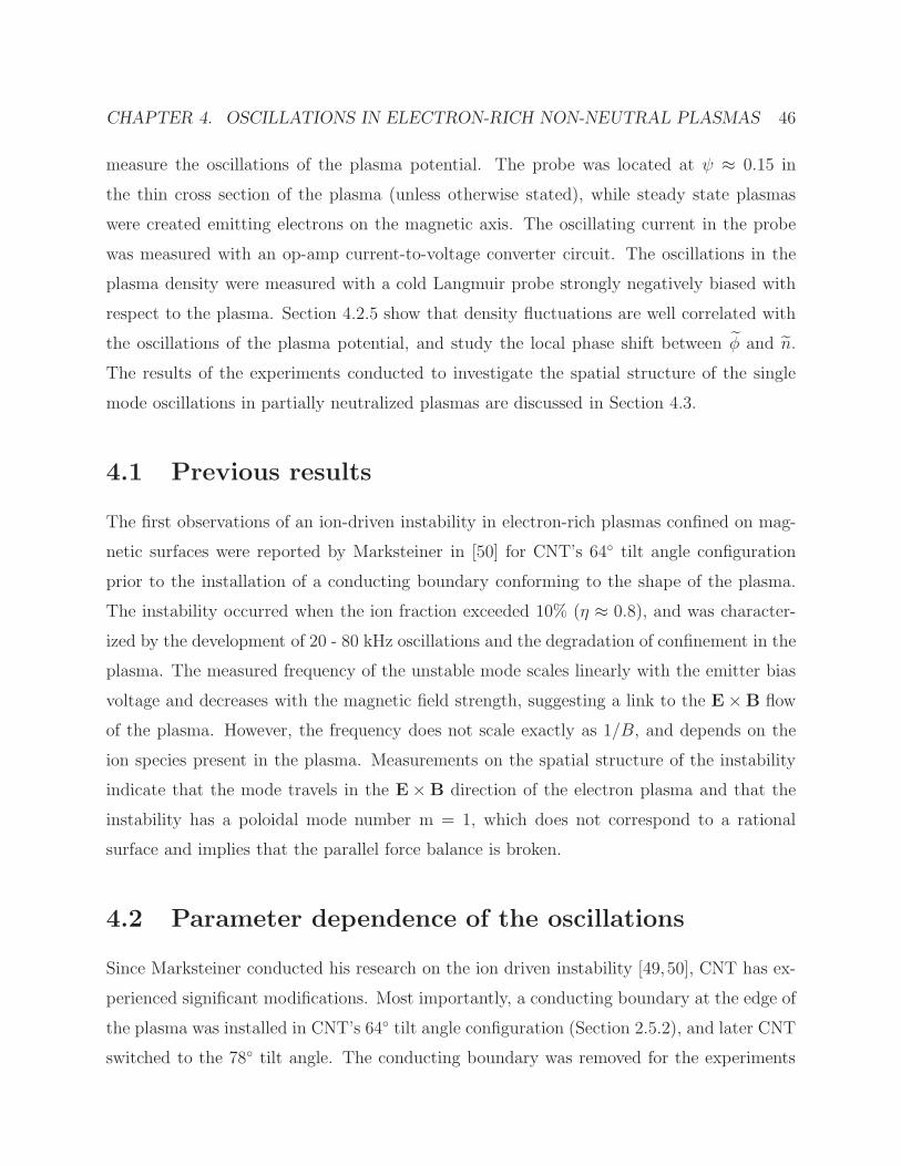
CHAPTER 4. OSCILLATIONS IN ELECTRON-RICH NON-NEUTRAL PLASMAS 46
measure the oscillations of the plasma potential. The probe was located at ψ ≈ 0.15 in
the thin cross section of the plasma (unless otherwise stated), while steady state plasmas
were created emitting electrons on the magnetic axis. The oscillating current in the probe
was measured with an op-amp current-to-voltage converter circuit. The oscillations in the
plasma density were measured with a cold Langmuir probe strongly negatively biased with
respect to the plasma. Section 4.2.5 show that density fluctuations are well correlated with
the oscillations of the plasma potential, and study the local phase shift between φ and n.
The results of the experiments conducted to investigate the spatial structure of the single
mode oscillations in partially neutralized plasmas are discussed in Section 4.3.
4.1 Previous results
The first observations of an ion-driven instability in electron-rich plasmas confined on mag-
netic surfaces were reported by Marksteiner in [50] for CNT’s 64 tilt angle configuration
prior to the installation of a conducting boundary conforming to the shape of the plasma.
The instability occurred when the ion fraction exceeded 10% (η ≈ 0.8), and was character-
ized by the development of 20 - 80 kHz oscillations and the degradation of confinement in the
plasma. The measured frequency of the unstable mode scales linearly with the emitter bias
voltage and decreases with the magnetic field strength, suggesting a link to the E×B flow
of the plasma. However, the frequency does not scale exactly as 1/B, and depends on the
ion species present in the plasma. Measurements on the spatial structure of the instability
indicate that the mode travels in the E×B direction of the electron plasma and that the
instability has a poloidal mode number m = 1, which does not correspond to a rational
surface and implies that the parallel force balance is broken.
4.2 Parameter dependence of the oscillations
Since Marksteiner conducted his research on the ion driven instability [49,50], CNT has ex-
perienced significant modifications. Most importantly, a conducting boundary at the edge of
the plasma was installed in CNT’s 64 tilt angle configuration (Section 2.5.2), and later CNT
switched to the 78 tilt angle. The conducting boundary was removed for the experiments

CHAPTER 4. OSCILLATIONS IN ELECTRON-RICH NON-NEUTRAL PLASMAS 47
in the 78 configuration (the shape of the plasma is rather different in the three magnetic
configurations in which CNT can operate, and the 64 conducting boundary could not be
reused for the 78 tilt angle).
The parameter dependence of the detected oscillations in electron-rich non-neutral plas-
mas is explored in this Section, focusing on the effects of the conducting boundary and the
magnetic configuration.
4.2.1 Effect of the conducting boundary at the plasma edge
The installation of a conducting boundary sets the 0 V electrostatic condition at the edge of
the plasma (otherwise, the 0 V condition is set at the surface of the vacuum chamber and the
IL coils). Hence, the conducting boundary results in an increased potential drop across the
plasma for a given emitter bias, which in turn leads to three times denser electron plasmas.
Results with the conducting boundary installed confirm the presence of an instability in
partially neutralized plasmas. However, as described in Section 3.6, the behavior of the
oscillations is significantly different compared to previous results without the conducting
boundary (Section 4.1).
In order to evaluate the effect of the conducting boundary on the oscillations observed
in partially neutralized plasmas, the fluctuations of the plasma were measured for a set of
pressure and B field scans where the emitter bias voltage was held at -60 V. This emitter
bias was chosen to reproduce the voltage drop across the plasma when emitting electrons
at -200 V before the installation of the conducting boundary [43]. Higher ion contents are
required to destabilize the plasma with the boundary at the plasma edge (the threshold for
instability with the boundary installed is ni ≈ 1012m−3, which corresponds to η ≈ 0.2).
The parameter dependence of the oscillations is very similar for both electrostatic boundary
conditions. When the conducting boundary is installed, the frequency of the dominant
mode also scales linearly with the plasma potential (φp) and decreases with the magnetic
field strength. Fig. 4.1 shows that the measured frequency of the fluctuations scales close to
linear with φp/B, indicating that the physics behind these oscillations may be identical to
the situation without the conducting boundary. However, an offset frequency of a few kHz
is observed at φp/B = 0, which does not agree with a purely E×B rotation of plasma.

CHAPTER 4. OSCILLATIONS IN ELECTRON-RICH NON-NEUTRAL PLASMAS 48
Figure 4.1: Frequency of the dominant modes vs φp/B while emitting electrons at low bias
voltages (φe between -40 and -100 V) with the conducting boundary installed. Neutral
pressure of N2 between 8 · 10−7 and 8 · 10−6 Torr and B field strengths ranging from 0.02 to
0.07 T.

CHAPTER 4. OSCILLATIONS IN ELECTRON-RICH NON-NEUTRAL PLASMAS 49
Figure 4.2: Power spectrum of the signal on a floating emissive probe vs. degree of non-
neutralization. N+2 − e− plasmas, φe = −200 V, 64 configuration. Left: B = 0.02 T. Right:
B = 0.08 T
4.2.2 Dependence on η, φplasma and B field strength
The behavior of partially neutralized plasmas is rather different when operating at emitter
bias voltages more negative than−100V with the 0 V boundary condition at the plasma edge.
The power spectrum of the oscillations in a floating emissive probe shows multiple peaks and
broad band behavior (Figs. 3.18 and 4.2-left). However, for magnetic field strengths above
0.04 T and degrees of non-neutralization between ∼ 0.001 and 0.1 partially neutralized
plasmas exhibit oscillations with a dominant mode between 20 and 100 kHz (Fig. 4.2-right).
Although the amplitude of the oscillations increases significantly when η decreases down
to 10−3 for all the emitter bias voltages and magnetic field strengths explored (as seen in
Fig. 3.17), the frequency of the dominant mode does not present a strong dependency on η
(Fig. 4.2-right). A slight decrease of the frequency is observed as the ion content increases,
due to the decoupling of the plasma potential from the emitter bias voltage in this range of
degrees of neutralization (Fig. 4.3). This is observed for the whole range of B field strengths
where this mode appears, and clearly the frequency of the mode does not scale like√ni,
which eliminates the possibility of having a sheath instability related to the ions [55].
Fig. 4.3 also shows that the measured frequency of the oscillations decreases with the B
field strength, but not as fast as 1/B. The frequency of the mode grows with |φp| but a clear

CHAPTER 4. OSCILLATIONS IN ELECTRON-RICH NON-NEUTRAL PLASMAS 50
Figure 4.3: Measured frequency of the dominant mode vs. pn. N+2 − e− plasmas, φe = −200
V, 64 configuration.
linear scaling is not observed for all the B fields explored (Fig. 4.4). However, experiments
conducted at constant φe/B ratio indicate that this mode may scale linearly with E/B
(Fig. 4.5-left). This hypothesis is confirmed in Fig. 4.5-right, implying that the single mode
oscillations observed in partially neutralized plasmas can be related to the E×B rotation.
Nevertheless, a ∼ 10 kHz offset can be also seen in Fig. 4.5-right for φp/B = 0, implying
that the detected mode it is not simply caused by the E×B flow. The linear dependency
of the mode frequency on φp/B breaks down at high emitter bias voltages and low magnetic
field strengths, or even no clear dominant mode is observed because the plasma presents
multimode or broadband behavior.
Results shown in Fig. 4.1 and 4.5-right are overlaid in Fig. 4.6. The measured frequency
of the dominant mode has the same linear scaling with E/B both in Fig. 4.1 and 4.5-
right, suggesting that the single mode detected in partially neutralized plasmas with the
conducting boundary installed might be identical to the ion-driven instability reported by
Marksteiner [50].

CHAPTER 4. OSCILLATIONS IN ELECTRON-RICH NON-NEUTRAL PLASMAS 51
Figure 4.4: Frequency of the detected mode as a function of the measured plasma potential.
N+2 − e− plasmas, 4 · 10−7 < pn < 2 · 10−6 Torr, 64 configuration.
4.2.3 Effect of different ion species
The behavior of the oscillations in partially neutralized N+2 −e− plasmas has been described in
Section 4.2.2, but it remained to be studied how the introduction of ions with different masses
affects the oscillations. Experiments were conducted for partially neutralized Ar+ − e−,
He+−e− plasmas in the 64 tilt angle configuration with the conducting boundary installed,
exploring the dependence of the mode on the degree of neutralization, electric, and magnetic
field strength.
As the ion content increases in the plasma, an unstable mode also develops in Ar+ − e−and He+ − e− plasmas 1. The oscillations in both Ar+, He+ plasmas present an almost
identical behavior compared to N+2 plasmas. The frequency of these fluctuations has negli-
gible dependence on η, scales close to linear with φp, and decreases with the magnetic field
strength. This is particularly evident in the case of He+ (Fig. 4.7). Fig. 4.8 summarizes
how the frequency of this mode depends on E/B for Ar+, He+ and N+2 . When lighter ion
1In Ar+ plasmas the mode is clearly observed for neutral pressures between 10−7 and 6 · 10−7 Torr, and
−250 < φe < −50 V. In He+ plasmas, for neutral pressures between 3 · 10−6 and 2 · 10−5 Torr.

CHAPTER 4. OSCILLATIONS IN ELECTRON-RICH NON-NEUTRAL PLASMAS 52
freq vs. pn (constant φe/B) freq vs. φp/B
Figure 4.5: E/B scaling of the dominant mode in partially neutralized plasmas. N+2 −
e− plasmas, 64 configuration. Left: Measured frequency as a function of pn at constant
φe/B ratio. The measured frequency decreases slightly as φp starts decoupling from φe
(Section 3.3). Right: Measured frequency vs. φp/B. The frequency of the mode scales
linearly with φp/B. However, a ∼ 10 kHz offset is observed at φp/B = 0, which does not
agree with a purely E×B rotation.
Figure 4.6: Frequency of the dominant mode in partially neutralized plasmas vs. E/B with
the conducting boundary installed in the 64 configuration. Figs. 4.1 and 4.5-right overlaid.

CHAPTER 4. OSCILLATIONS IN ELECTRON-RICH NON-NEUTRAL PLASMAS 53
freq vs. φp (B = 0.02 T) freq vs. B field (φe = −200 V)
Figure 4.7: Dependence of the measured frequency of the mode on the plasma potential
(left) and the magnetic field strength (right). He+ − e− plasmas in the 64 configuration.
species (He+) are introduced in the plasma, slightly higher frequencies are measured, but in
all cases the measured frequency scales close to linear with E/B.
When an additional rod is inserted in the thin cross section of the plasma, the shape of
the ion density profile is not affected, but the ion density at a given neutral pressure is halved
everywhere in the plasma [49]. The set of experiments described in Section 3.1.3 of [49] were
reproduced here to study how the presence of an additional ceramic rod in the plasma affects
the threshold for instability when the conducting boundary was installed. The results of the
experiments with two ceramic rods are identical for both electrostatic boundary conditions
at the edge of the plasma: the pressure threshold for instability occurs at approximately
two times higher pressure when a second rod is present, which approximately corresponds
to the same ion content threshold as when a single rod is present. This confirms that the
presence of ions is responsible of the appearance of spontaneous oscillations in electron-rich
non-neutral plasmas.
4.2.4 Effect of the magnetic configuration
The three tilt angles of operation in CNT represent three rather different shapes of the
plasma and explore three generic shear configurations. The results described so far in this

CHAPTER 4. OSCILLATIONS IN ELECTRON-RICH NON-NEUTRAL PLASMAS 54
Figure 4.8: Measured frequency vs. E/B for Ar+ − e−, He+ − e− and N+2 − e− plasmas in
partially neutralized plasmas. 64 configuration.
Section refer to the 64 configuration, but CNT’s tilt angle was switched to 78 in the course
of this thesis. The 64 configuration presents reversed shear, while the 78 tilt angle is
essentially shear free.
Unstable fluctuations were also detected in the 78 configuration when the ion content
exceeds a certain threshold and the plasma starts decoupling from the emitter bias. These
oscillations present a dominant peak between 20 and 70 kHz for 10−7 ≤ pn ≤ 10−6 Torr
(Fig. 4.9). The amplitude and frequency of the oscillations observed in partially neutralized
plasmas are lower in the 78 configuration, probably due to the smaller potential drop across
the plasma when the 0 V boundary condition is set by the chamber and the coils. The
frequency of these fluctuations scales linearly with φp, but does not have a clear 1/B depen-
dence. Fig. 4.10 shows that the measured frequency of the mode scales reasonably well with
E/B. It seems also that the dominant mode switches to a higher frequency harmonic for high
φp/B ratios. Hence, these experiments confirm that partially neutralized plasmas behave
quite similarly in both stellarator configurations studied so far, despite having completely
different shape and magnetic shear.

CHAPTER 4. OSCILLATIONS IN ELECTRON-RICH NON-NEUTRAL PLASMAS 55
Figure 4.9: Power spectrum of the signal on a floating emissive probe vs. neutral pressure.
N+2 − e− plasmas, B = 0.08 T, φe = −200 V, 78 configuration.
Nevertheless, notable differences were appreciated in the 78 configuration. For instance,
when the plasma abruptly decouples from the emitter bias (0.2 < φp/φe < 0.8, corresponding
to 10−6 < pn < 5·10−6 Torr), the power spectrum also broadens considerably, but a dominant
peak can always be observed in this regime at high magnetic field strengths (B ≥ 0.06 T)
for the 78 tilt angle (Fig. 4.9). The frequency of this oscillation decreases as the degree of
non-neutralization gets closer to quasi-neutrality (in this regime the plasma potential is very
sensitive to the degree of neutrality). And the dominant mode seems to jump to a higher
frequency when a certain degree of neutrality is exceeded, probably indicating a higher spatial
mode number of the oscillations (see Fig. 4.9 between 10−6 and 10−5 Torr). This hypothesis
will be confirmed in the Sections exploring the spatial structure of the modes (Section 4.3 for
partially neutralized, and Section 5.3 for quasi-neutral plasmas), showing that the ion-driven
oscillations observed in electron-rich non-neutral plasmas present a poloidal mode number
m = 1, while the quasi-neutral oscillations align with the field lines and exhibit a m = 3
poloidal structure.

CHAPTER 4. OSCILLATIONS IN ELECTRON-RICH NON-NEUTRAL PLASMAS 56
Figure 4.10: Measured frequency of the oscillations in partially neutralized plasmas vs φp/B
in the 78 configuration (electron-rich N+2 plasmas, pn = 3.1 · 10−7 Torr, −400 ≤ φe ≤ −100
V).
4.2.5 Local phase shift between density and potential fluctuations
Experiments were also conducted to measure the local phase difference between density and
potential oscillations in CNT, since this phase shift between n and φ usually determines
the nature of the oscillation in quasi-neutral plasmas [38]. These experiments were only
performed in the 78 configuration.
Method
A relatively simple method to determine the local phase shift between n and φ involves the
use of two probes in two different sets of experiments. A series of experiments measured
the oscillations of the potential by floating an emissive filament at location 2 of the nw4
probe array (which corresponds to ψ ≈ 0.15 in the thin cross section of the plasma), and
another set of experiments reproduced the same experimental conditions but now replacing
the floating emissive filament by an ion probe to measure the density oscillations at the same
location. A different floating emissive filament was also used in both sets of experiments to

CHAPTER 4. OSCILLATIONS IN ELECTRON-RICH NON-NEUTRAL PLASMAS 57
Emitter circuit I-V converter
Figure 4.11: Phase shift introduced by the electronic circuits used to measure the fluctuations
in the plasma.
measure the potential oscillations at location 3 of the nw4 probe array (ψ ≈ 0.45), and use
the signal in this probe as the reference to correlate the density and potential fluctuations
in nw4 2.
The circuits used in these experiments were calibrated to determine the phase shift intro-
duced by the electronics and correct the measurements accordingly. The emitter circuit used
to measure the current fluctuations in the ion probe does not introduce any phase shift for
frequencies below 10 kHz, but delays more than π rad signals above 100 kHz (Fig. 4.11-left).
The phase response of the I-V converter that measured the plasma potential oscillations in
the emissive probes is shown in Fig. 4.11-right.
The real phase shift between the signals measured in nw4 2 and 3 (α) can be determined
from the measured phase difference (α′) and the phase delays introduced by the electronics
(δ1 and δ2), as shown in Fig. 4.12:
α = α′ − δ1 + δ2 (4.1)
The Fourier power spectrums of the fluctuations detected in nw4 2 and 3 are compa-
rable, and clear sinusoidal oscillations proportional to the plasma density and potential are
detected in partially neutralized and quasineutral plasmas. The cross-correlation between n
and φ also confirms that density fluctuations are well correlated with the oscillations of the

CHAPTER 4. OSCILLATIONS IN ELECTRON-RICH NON-NEUTRAL PLASMAS 58
Figure 4.12: Determination of the phase difference between the signals measured in nw4 2
and 3. The dashed lines represent the measured signals, and solid lines are the real signals.
α is the real phase difference between the oscillations, α′ is the measured phase shift, and δ1
and δ2 are determined through the calibration of the electronics (Fig. 4.11)
plasma potential.
The dominant frequency of the cross-correlation between the density (measured in nw4
2) and the potential (nw4 3) oscillations are shown in Fig. 4.13-right for a pressure and
a B field scan. In Fig. 4.13-right two regions can be identified with the usual scalings: 1)
partially neutralized plasmas present oscillations between 25 and 35 kHz whose frequency
decreases slightly with the magnetic field strength, and 2) quasineutral plasmas exhibit lower
frequency oscillations (1 - 8 kHz) and its frequency increases with the magnetic field strength.
An identical behavior is observed in the dominant frequency of the cross-correlation between
the potential fluctuations measured in nw4 2 and nw4 3 as the degree of neutralization and
the magnetic field strength are varied (Fig. 4.13-left).
The phase difference between the signal in two probes was extracted using the cross-
correlation function [37]. Since the phase of the cross-correlation is a function of the fre-
quency, the value of phase shift shown in this Section corresponds to the dominant frequency
of the cross-power spectrum.

CHAPTER 4. OSCILLATIONS IN ELECTRON-RICH NON-NEUTRAL PLASMAS 59
Dominant freq cross-correlation φ2 - φ3 Dominant freq cross-correlation n2 - φ3
Figure 4.13: Left: Dominant frequency of the cross correlation between the potential fluc-
tuations measured in nw4 2 and nw4 3 as the degree of neutralization and the B field are
varied. Right: Dominant frequency of the cross correlation between the density (measured
in nw4 2) and the potential (nw4 3) fluctuations as the degree of neutralization and the B
field strength are varied. (N+2 - e− plasmas, φe = −200 V).
Results
In partially neutralized plasmas, the measured oscillations of the plasma potential (φ) in
nw4 2 present a modest delay with respect to nw4 3 (−45 on average, see Fig. 4.14-left
for a series of B field and φe sweeps). Fig. 4.14-right shows that the average phase difference
between the density fluctuations (n) in nw4 2 and φ in nw4 3 is −55. Thus, n and φ are
very close to being in phase 2 at the location of the probe nw4 2 (which corresponds to
ψ ≈ 0.15).
In CNT’s electron-rich plasmas the equilibrium distribution function of electrons on each
magnetic surface is ne = N(ψ) exp (eφ/Te(ψ)) [59]. Therefore, since the plasma is subjected
to small oscillatory perturbations (|eφ|/Te < 1, see Fig. 3.19), φ and n are predicted to be
in phase if the electron fluid remains in equilibrium, which agrees with the experimental
observations.
2There is better than 95% confidence that the phase shift between n and φ lies within the interval
−10 ± 69

CHAPTER 4. OSCILLATIONS IN ELECTRON-RICH NON-NEUTRAL PLASMAS 60
Phase φ2 - φ3 Phase n2 - φ3
Figure 4.14: Left: Phase difference between the potential fluctuations measured in nw4 2
and nw4 3. Right: Phase difference between the density (measured in nw4 2) and the
potential (nw4 3) fluctuations. The dashed blue line represents the average phase shift, and
the ±2σ confidence interval is given by the two red dotted lines. Partially neutralized N+2 -
e− plasmas, −300 < φe < −150 V, 0.04 < B < 0.08 T.
4.3 Spatial Structure
4.3.1 Theoretical considerations
Equilibrium for a pure electron plasma in a stellarator is in a minimum energy state [58], and
parallel force balance pertains to a whole magnetic surface [59]. Any macroscopic motion
of the plasma away from the magnetic surfaces implies the breaking of the parallel force
balance [59].
In a stellarator, the rotational transform (ι) describes the poloidal twist of the field lines
around the torus [7]. A rational magnetic surface is a surface where ι is equal to a low
order rational number ι = n/m, and the field lines close on themselves after n poloidal and
m toroidal transits around the torus [9]. Therefore, perturbations can exist in a resonant
rational surface without breaking the parallel force balance.
CNT’s ion-driven instability was first characterized by Marksteiner in [50] for the 64
tilt angle configuration prior to the installation of a conducting boundary at the edge of the
plasma. A set of capacitive probes around the thick poloidal cross section of the plasma

CHAPTER 4. OSCILLATIONS IN ELECTRON-RICH NON-NEUTRAL PLASMAS 61
was used to determine that the azimuthal mode number of these oscillations was m =
rkθ = 1. This result posed a challenge to theory, since an azimuthal mode m = 1 mode
had been observed in Penning and pure-toroidal traps [17, 19, 24, 76, 79], but this oscillation
was predicted to be damped by the magnetic surfaces much faster than the period of an
oscillation [50, 59] (the ι profile of CNT for these experiments grows monotonically from
ι(ψ = 0) = 0.12 to ι(ψ = 1) = 0.23). Hence, in CNT’s 64 configuration the magnetic
surfaces are not able to stabilize the ion-driven instability, and the parallel force balance
is broken. This was, indeed, the first time that an instability non-resonant with a rational
surface was observed in a stellarator.
There are still interesting questions that remain to be answered regarding the charac-
terization of the ion-driven instability in a stellarator, most importantly: the effect of the ι
profile, and the determination of the toroidal mode number (n) of the oscillations.
The 78 tilt angle presents an almost flat ι ≈ 1/3 profile [41]. This Section will explore
whether the ion-driven mode aligns with the magnetic field lines in the 78 configuration
(and presents a resonant m = 3 structure) or, on the contrary, this instability also breaks
parallel force balance even in the presence of low order rational surfaces. The magnetic shear
plays an important role in suppressing diocotron instabilities [40], therefore experiments in
the 78 tilt angle configuration can provide valuable information for the understanding of
this instability.
In the infinite conductivity approximation Ohm’s law is simply E + u × B = 0. The
consequences of infinite conductivity in Magnetohydrodynamics (MHD) are that the plasma
is tied to the magnetic field lines, and the magnetic flux through any closed contour moving
with the plasma is conserved [27]. The diocotron mode in a pure toroidal trap presents a
m = 1, n = 0 structure [75]. However, stellarators must have a finite poloidal flux through
the hole of the torus, which will remain unchanged if integrated through an area bounded
by any closed tube moving with the E ×B drifting plasma. Therefore, the ion-driven mode
in a stellarator is predicted to have a toroidal mode number n > 0 to conserve the poloidal
magnetic flux (even if the parallel force balance is broken).
The experiments explained below investigate the spatial structure of the ion-driven mode
detected in electron-rich non-neutral plasmas for the 78 tilt angle configuration, and study
the influence of the ι profile in the spatial structure of the instability.

CHAPTER 4. OSCILLATIONS IN ELECTRON-RICH NON-NEUTRAL PLASMAS 62
4.3.2 Experimental results
The toroidal and poloidal structure of the ion resonant mode in the 78 configuration was
measured with two perpendicular arrays of capacitive probes (described in Section 2.5.2).
The oscillations detected in the capacitive probes are very well correlated with the signal in
the floating emissive probe. Indeed, it has been observed that the measured frequency of
the oscillations is exactly the same at different radial locations (Section 4.2.5) and at edge
of the plasma (measured with the capacitive probes), so the ion resonant mode is a global
instability.
The poloidal array of capacitive probes consists of 5 copper disks located around the
thick poloidal cross-section of the plasma (ϕ = 90), providing enough spatial resolution to
determine the poloidal mode number of the oscillation. The layout of the poloidal capacitive
probes can be seen in Fig. 4.15, along with the measured phase shift of the signal in each
probe relative to TP 3. The phase difference between the image charge measurements
corresponds to the phase of the dominant mode of the cross-correlation power spectrum [37].
Fig. 4.15 also shows the predicted phase shift of a m = 1, 2, and 3 mode assuming a circular
cross-section of the plasma at ϕ = 90. The mode travels in the E ×B direction of rotation
of the plasma, and all the measured phase differences are consistent with a m = 1 poloidal
mode structure, except the recorded phase shift on probe P4, which always lies between the
predicted m = 1 and m = 2 phase. It is not understood why the measurements at P4 do not
fit the predicted m = 1 mode as well as the rest of the probes. Nevertheless, the experiment
was performed at different emitter bias voltages (−300 < φe < −150 V), and magnetic field
strengths (0.04 < B < 0.08 T), providing enough evidence to conclude that the mode is m
= 1.
Since the 78 tilt angle presents an almost flat ι ≈ 1/3 profile [41], it was originally
thought that the ion-driven mode might align with the magnetic field lines in this configura-
tion and have a resonant m = 3 poloidal structure. However, the phase shift measurements
give strong evidence to suggest that ion-driven instability in the 78 configuration has a
m = 1 mode number, which is the same as that of ion-driven instabilities in Penning and
pure-toroidal traps [17, 24, 76, 79] and CNT’s 64 conf. [50], and implies that the ion insta-
bility breaks parallel force balance in a stellarator even in the presence of low order rational

CHAPTER 4. OSCILLATIONS IN ELECTRON-RICH NON-NEUTRAL PLASMAS 63
Figure 4.15: Measured phase shift of the ion-driven mode detected on the poloidal capacitive
probes. The phase on probe TP 3 is used as the reference. pn = 4 · 10−7 Torr of N2,
φe = −200 V, B = 0.08 T, 78 configuration.
surfaces.
The mechanism causing the violation of the parallel force balance in the stellarator is not
completely understood, but it might be due to the presence of an anisotropic ion pressure
tensor (←→p i) [6]. Largely unmagnetized ions are drawn electrostatically into the electron-rich
plasma without collisions, and the distribution function of ions is predicted to be non-
Maxwellian and anisotropic. The force balance of the ion fluid can be written as:
mini∂ui∂t
+ ∇ ·←→p i = eni( E + ui × B) (4.2)
where the ion fluid velocity is ui =∫vfid
3v, and the ion pressure tensor is←→p i =∫mivvfid
3v.
The expression for the electron force balance is analogous, but the electrons have negli-
gible inertia, are magnetized, and the pressure tensor is likely to be isotropic:
E + ue × B = −∇peene
(4.3)
The plasma force balance is obtained summing Eqs. 4.2 and 4.3:
mini∂ui∂t
+ ∇ ·←→p = e(ni − ne) E +j × B (4.4)

CHAPTER 4. OSCILLATIONS IN ELECTRON-RICH NON-NEUTRAL PLASMAS 64
where j ≡ eniui − eneue is the electrical current and ←→p = ←→p i + pe←→1 is the pressure
tensor. The anisotropic ←→p can modify parallel force balance in a way that an isotropic
pressure cannot, and might explain the existence of an ion-driven mode not aligned with the
magnetic field lines.
The toroidal structure of the oscillations was investigated with a set of 6 capacitive probes
which covered 105 along the toroidal angle of the torus (Fig. 4.16). The measured phase
difference of the image charge oscillations in each probe with respect to TP 3 is also shown in
Fig. 4.16, suggesting that the toroidal mode number of the oscillation is n = 0 (the predicted
phase shifts in Fig. 4.16 assumed a circular magnetic axis). Experiments at different emitter
bias voltages (−300 < φe < −150 V), and magnetic field strengths (0.04 < B < 0.08 T)
produced very similar results. In order to verify the n = 0 structure of the ion mode, an
additional capacitive probe was installed 180 away toroidally from probe TP 3, and the
phase difference between the two probes was measured. Fig. 4.17 shows that the signals in
two probes separated by 180 toroidally are nearly in phase for a series of φe and B field
sweeps (there is better than 95% confidence that the phase shift between the two probes is
within the interval 0.5± 0.6 rad).
Hence, there is strong evidence indicating that the spatial structure of the ion-driven
driven mode is m = 1, n = 0, which is identical to the diocotron mode detected in pure
toroidal traps [75]. This implies that the global ion mode observed in CNT is not aligned
with the magnetic field lines, and the poloidal magnetic flux is not conserved in a close
tube of plasma moving with this mode. It is believed that the presence of an anisotropic
pressure tensor in the plasma force balance (Eq. 4.4) might also explain the n = 0 structure
of this mode (since it introduces a ∇ · ←→p term that is usually neglected in the ideal MHD
approximation of Ohm’s law).
4.4 Multi-mode oscillations in partially neutralized plas-
mas.
This thesis focuses on the investigation of the single mode oscillations observed in partially
neutralized and quasi-neutral plasmas (Sections 4.2 and 5.2 respectively). However, the

CHAPTER 4. OSCILLATIONS IN ELECTRON-RICH NON-NEUTRAL PLASMAS 65
Figure 4.16: Measured phase shift of the ion-driven mode detected on the toroidal capacitive
probes. The phase on probe TP 3 is used as the reference. pn = 4 · 10−7 Torr of N2,
φe = −200 V, B = 0.08 T, 78 configuration.
presence of broadband fluctuations and the jumps between equilibrium states are also very
characteristic of partially neutralized plasmas. A summary of the first observations of multi-
mode oscillations in partially neutralized plasmas is presented in this Section with the aim
of inspiring future research on this largely unexplored regime of plasma physics. A detailed
study of the physics behind this behavior is outside of the scope of this thesis, and will not
be discussed in depth.
4.4.1 Multi-mode oscillations
There are two regions where partially neutralized plasmas present multi-mode oscillations:
1) for degrees of non-neutralization between η = 0.1 and 0.01, and 2) for η ranging from
η = 0.01 to 10−4 (Fig. 3.18).
The first kind of multi-mode oscillations (0.1 > η > 0.01) are only observed when the
plasma contains essentially unmagnetized ions (such as N+2 at 0.02 T), bouncing chaotically
in the electron-rich plasma. The dominant peaks of the Fourier Spectrum (typically < 100
kHz) are in the same range as the ion bounce frequency [49] and the E × B rotation of the

CHAPTER 4. OSCILLATIONS IN ELECTRON-RICH NON-NEUTRAL PLASMAS 66
Figure 4.17: Measured phase difference between two capacitive probes separated 180
toroidally from each other. The phase on probe TP 3 is used as the reference. The dashed
blue line represents the average phase shift, and the ±2σ confidence interval is given by the
two red dotted lines. Partially neutralized N+2 - e− plasmas, pn = 4 · 10−7 Torr, 78 configu-
ration. Measurements performed for a series of φe, and B field sweeps: −300 < φe < −150V, 0.04 < B < 0.08 T.

CHAPTER 4. OSCILLATIONS IN ELECTRON-RICH NON-NEUTRAL PLASMAS 67
plasma, but it is unclear if the multiple harmonics detected in the spectrum are part of the
ion driven instability or are a different kind of oscillation. It is not understood either how the
fact that ε⊥ < 0 for B < 0.04 T (Fig. 3.15) may affect the multiple peak oscillations. The
multi-mode behavior of this regime degenerates into a single mode when more magnetized
ions (rLi < 〈a〉) are introduced in the plasma (see Section 4.2). The amplitude of the
oscillations grows as more ions are introduced into the plasma (Fig. 3.17), and the plasma
is always more unstable when multiple modes are excited. For a given η, the RMS of the
fluctuations is higher when the plasma exhibits multiple modes than when only the single
mode ion-driven oscillation is excited.
Multiple peak oscillations are also detected when η ranges from η = 0.01 to 10−4. This
regime is very rich in relevant changes occurring in the plasma: the potential profiles decouple
rather abruptly from the emitter bias, the onset of the saturation of the charge loss rate is
reached at η ≈ 3 · 10−3, and the maximum amplitude and broadest power spectrum of the
oscillations are observed simultaneously at η ≈ 5 · 10−3. Multiple mode oscillations are
always observed between η = 0.01 and 10−4 independently of the degree of magnetization of
the ions. In this range of η, most of the power of the oscillations is normally contained in a
broad dominant peak between 100 and 200 kHz, but also narrower peaks related to the E×Brotation of the plasma are observed. The frequency of these E × B peaks decreases as the
degree of non-neutralization approaches quasi-neutrality (Fig. 3.18) due to the decoupling
of the plasma from the emitter bias. The power spectrum of the oscillations in this regime
narrows down for stronger magnetic field strengths and degrees of non-neutralization closer
to quasi-neutral.
4.4.2 Jumps between equilibrium states
Rather abrupt changes in the emission current and the plasma potential occur when the ion
content exceeds 5 · 1013 m−3 (corresponding to η < 10−2) (see more details in Section 3.3.2).
Fig. 4.18 shows that sometimes during the same shot the plasma switches back and forth
between a stable equilibrium state (characterized by a plasma potential close to the emitter
bias and low emission currents) and a metastable state (in which the plasma is detached
from the emitter bias and the emission current is significantly higher). The jumps between

CHAPTER 4. OSCILLATIONS IN ELECTRON-RICH NON-NEUTRAL PLASMAS 68
equilibrium states in partially neutralized plasmas typically occur in ∼ 100 ms, which is a
timescale much slower than the parallel equilibration of the plasma. The timescale of the
jumps observed in the emission current and the floating potential are in very good agreement,
and these measurements were performed with completely different electronic circuits. Also,
the fastest sudden change in the voltage that the current source circuit is able to detect
is 20 V/ms, while the slopes measured between equilibrium states were ∼ 0.6 V/ms (i.e.,
the electronic circuits used are sufficiently fast to measure the time constant of the jumps
between two equilibrium states).
Transport jumps have been previously observed in CNT’s pure electron plasmas [30], but
in that case the potential profiles of the two equilibrium states were only slightly different.
Hence, the physics behind the two equilibrium states in partially neutralized plasmas appears
to be very different from the transport jumps of pure electron plasmas. Since the separation
of the plasma potential from the emitter bias is caused by the presence of a finite ion
fraction, not due to an emission limit (see Section 3.3.2), the jumps between states in partially
neutralized plasmas could be explained in terms of a process that enhances ionization. The
plasma becomes denser and hotter as we approach quasi-neutrality (Chapter 3), increasing
the ionization rate in the plasma, which might lead to a non-linear self-enhancing process.
The jumps between equilibrium states here occur when the plasma density is comparable
to the density limit of non-neutral plasmas confined in magnetic surfaces [8], however the
physics involved in this case also seem to be different.
4.5 Summary and discussion
The single mode oscillations detected in electron-rich non-neutral plasmas have many char-
acteristics in common with the first observations of the ion-driven fluctuations reported by
Q.R. Marksteiner et al. in Ref. [50]. In all the different configurations studied so far (64
conf. with and without a conducting boundary, and 78 tilt angle), CNT’s electron-rich plas-
mas exhibit a 20 - 100 kHz mode related to the E×B rotation when a certain ion threshold
is exceeded. The measured frequency of the mode is not just determined by ωE×B, but also
the depends weakly on the ion species introduced: when the mass of the ions introduced in
the plasma is increased by a factor of 10 (Ar+ vs. He+), 30% lower frequencies are typically

CHAPTER 4. OSCILLATIONS IN ELECTRON-RICH NON-NEUTRAL PLASMAS 69
Figure 4.18: Evolution of the emission current (top) and the floating potential at ψ ≈ 0.14
(bottom) as function of time for two different shots: a) φe = −200 V, B = 0.08 T and
pn = 2 · 10−6 Torr; and b) φe = −100 V, B = 0.04 T and pn = 4.2 · 10−6 Torr. The plasma
switches between two equilibrium states.
measured for a given φp/B ratio (Fig. 4.8). An offset frequency of ∼ 10 kHz is also observed
at φp/B = 0 (Fig. 4.5-right), which does not agree either with a purely E×B rotation of
plasma.
The spatial structure of the oscillations for the 78 tilt angle was measured with two
perpendicular arrays of capacitive probes (Fig. 2.2). The ion-driven mode is a global mode
of the plasma which travels in the direction of the E×B drift, and exhibits a m = 1 poloidal
mode number for both the 64 [49, 50] and the 78 configurations (Fig. 4.15). This implies
that CNT’s ion resonant instability cannot be stabilized by the magnetic surfaces, even when
low number rational magnetic surfaces are present (78 tilt angle). These oscillations are
not aligned with the magnetic field lines, and the mode breaks parallel force balance.
The toroidal mode number (n) of the ion-driven oscillations in a stellarator was measured
for the first time in this thesis. The mode was determined to be n = 0 for the 78 tilt angle
(Fig. 4.16), which is identical to the diocotron mode detected in the absence of magnetic
surfaces (m = 1, n = 0 structure in pure toroidal traps [75]), and indicates that the poloidal
flux is not conserved in a close tube of plasma moving with the ion-resonant mode. It is

CHAPTER 4. OSCILLATIONS IN ELECTRON-RICH NON-NEUTRAL PLASMAS 70
possible that the presence of an anisotropic pressure tensor in the plasma force balance
(Eq. 4.4) might explain the apparent breaking of parallel force balance, and the violation of
the conservation of poloidal magnetic flux.
One of the most significant differences between the results presented in this thesis and [49,
50] is the observation of two rather different regimes of oscillations in partially neutralized
plasmas: 1) the single mode ion-resonance instability, and 2) multi-mode / broadband power
spectrum oscillations. In the experiments conducted for this thesis, single mode oscillations
were only detected for 0.1 > η > 0.01 at high B field strengths (B > 0.04 T) or when light
ion species (He+) are present in the electron-rich plasma. Hence, the presence of ions with
small ion gyro-radius (rLi < 〈a〉) seems to play an essential role in the development of a
single mode ion resonance instability. Multi-mode oscillations are observed for plasmas with
degrees of non-neutralization between 10−4 and 10−2, and also when largely unmagnetized
ions are present in the plasma for 0.1 > η > 0.01. The plasma is more unstable when
multiple modes are excited. The detected fluctuations always present broadband power
spectrum when the RMS of the oscillations and the charge loss rate reach the highest values
(Figs. 3.17 and 3.18).
Davidson’s publication [19] studies the effect of a finite ion Larmor radius in a non-neutral
plasma column, showing that the fundamental l = 1 diocotron mode is unaffected by the
value of the ion Larmor radius, but for l ≥ 2 azimuthal mode number, finite Larmor radius
effects can have a strong stabilizing influence. A detailed analysis of the ion motion in the
complicated geometry of CNT is provided in Chapter 6 of [49]. Ions exhibit a bouncing
motion as they are accelerated in the electron-rich plasma. As shown in Fig. 3.14, massive
ions (such as N+2 ) at low magnetic field strengths (B = 0.02 T) are largely unmagnetized
(rLi 〈a〉), the ion motion is highly chaotic in the plasma, and multiple modes are excited.
However, for N+2 at 0.1 T, the ion gyro-radius is smaller than the torus minor radius (rLi
〈a〉) and the ions turn around before they are accelerated all the way into the plasma.
Magnetized ions in CNT (such as, N+2 at 0.1 T, or H+
2 for 0.02 ≤ B ≤ 0.1 T) travel close
to the E × B velocity and excite the ion-resonant mode, which scales very close to linear
with E/B. The mechanism for instability of these oscillations seems to be identical to the
ion resonant instability observed in Penning traps [19], but for the complicated geometry of
CNT, the presence of magnetized ions traveling close to the E×B drift is essential for single

CHAPTER 4. OSCILLATIONS IN ELECTRON-RICH NON-NEUTRAL PLASMAS 71
mode behavior. Otherwise, broadband oscillations are detected in the plasma.

Chapter 5
Oscillations in CNT’s quasi-neutral
plasmas
Quasi-neutral plasmas are routinely used in CNT to produce visualizations of the magnetic
surfaces [12]. When the background neutral pressure in the chamber exceeds 10−5 Torr
(η < 10−5), the plasma emits sufficient light in the visible range to be seen even with the
naked eye. These visualizations are systematically used as a diagnostic for probe alignment,
and confirmation of the magnetic topology [12], but CNT’s quasi-neutral plasmas had not
been studied in depth in the past.
Section 5.1 of this Chapter summarizes the first equilibrium measurements of quasi-
neutral plasmas in CNT. The rest of the Chapter is devoted to the detailed characterization
of the spontaneous oscillations detected for degrees of non-neutralization η < 10−4. Sec-
tion 5.2 investigates the dependence of the mode on experimentally adjustable parameters,
and Section 5.3 presents the studies on the spatial structure of the oscillations, providing
fundamental information to understand the underlying physics behind CNT’s quasi-neutral
fluctuations.
72

CHAPTER 5. OSCILLATIONS IN CNT’S QUASI-NEUTRAL PLASMAS 73
5.1 Equilibrium measurements in quasi-neutral plas-
mas
The potential, temperature and density of quasi-neutral plasmas have been measured by
the interpretation of the signal in emissive and Langmuir probes using the same techniques
described in [42] for pure-electron plasmas in CNT. The presence of ions in quasi-neutral
plasmas simplifies some of these measurements (the density of quasi-neutral plasmas can be
determined through the ion saturation current [34], while the lack of ions in a pure electron
plasma makes the measurement of ne much harder [42]).
In the quasi-neutral regime the plasma potential profiles are completely decoupled from
the emitter bias voltage (0 < φp/φe < 0.1), and the magnetic field strength determines
the equilibrium. |φp| increases with the magnetic field strength (Fig. 3.13), and typically
higher |φe| are associated to slightly lower measured values of |φp|. The reader is referred to
Section 3.3 for a complete description of the potential measurements. Fig. 5.1 shows that the
electron temperature at ψ ≈ 0.15 ranges between 30 and 45 eV in the quasi-neutral regime,
but does not have a clear relationship with the B field strength.
The power supplies used to bias our probes cannot handle the ion saturation currents
collected by a 7.4 cm2 ion probe in the quasi-neutral regime (this ion probe was originally
installed for the determination of ni in electron-rich plasmas, see Section 3.1). Instead, for
quasi-neutral plasmas a small cold filament (φ = 0.7mm, L = 3 mm) is used as an ion probe
(enough signal is collected by the filament, and Isat does not exceed the technical limits of the
power supplies). Isat is determined as the current at which the probe filament is 100 V more
negative than the local plasma potential. The Bohm sheath criterion was used to calculate
the density profiles shown in Fig. 5.2. The plasma density is slightly higher at stronger
B fields, and a centrally peaked density profile is always measured in CNT’s quasi-neutral
plasmas (Fig. 5.2). The Debye length in this regime is λD 1mm, which is more than one
order of magnitude smaller than λD for CNT’s pure-electron plasmas [43].

CHAPTER 5. OSCILLATIONS IN CNT’S QUASI-NEUTRAL PLASMAS 74
Figure 5.1: Measured Te at ψ ≈ 0.15 vs. B field strength in quasi-neutral plasmas. φe = −200V, pn = 2 · 10−5 Torr of N2. 78
configuration.
Figure 5.2: Measured density profiles in the nw4 probe array for B = 0.02 T, B = 0.04 T,
B = 0.06 T, and B = 0.08 T. Quasi-neutral plasmas. φe = −200 V, pn = 2 · 10−5 Torr of N2.
78 configuration.

CHAPTER 5. OSCILLATIONS IN CNT’S QUASI-NEUTRAL PLASMAS 75
5.2 Parameter dependence of the oscillations
In contrast to pure electron plasmas, quasi-neutral plasmas in CNT are characterized by
weak electric fields (the plasma comes closer to the E field set by ambipolarity). As plasmas
evolve to quasi-neutrality (η < 10−5), the power spectrum of the fluctuations narrows down
and its amplitude decreases until the oscillations settle into a steady state with approximately
constant amplitude and a single dominant frequency between 1 and 20 kHz.
This Section gives an overview on the possible mechanisms that might be driving these
oscillations, studies the dependence of the frequency and amplitude of the mode on ex-
perimentally adjustable parameters, investigates the local phase shift between density and
potential fluctuations, and presents the frequency profile of the oscillations at different radial
locations across the plasma.
5.2.1 Theoretical considerations
It is unlikely that the driving mechanism of CNT’s quasineutral mode is the same ion reso-
nance that we see in electron-rich non-neutral plasmas (the ion resonant instability is stable
in quasi-neutral plasmas [18, 19]).
The ratio of plasma pressure to magnetic pressure (β) is very low in CNT’s quasi-neutral
plasmas. Other quasi-neutral stellarators estimate the average β of the plasma (〈β〉) frommeasurements of the magnetic flux generated by the diamagnetic or the Pfirsch-Schluter
currents [53, 66]. 〈β〉 ≤ 2% is typical in other quasi-neutral stellarators [35, 78]. However,
in CNT the plasma currents produce a negligible perturbation to the vacuum magnetic
field created by the coils, and based on the equilibrium measurements, 〈β〉 is at least threeorders of magnitude lower than in other stellarators. Therefore, it is very unlikely that
the spontaneous mode detected in CNT’s quasi-neutral plasmas is driven by some MHD
instability, that usually limit the maximum achievable β in a stellarator. Also, the detected
oscillations travel at a velocity much slower than the Alfven speed, vA = B/√miniµ0 [27]
(in CNT vA ≈ 0.01c, where c is the speed of light in vacuum).
Low-β plasmas confined in toroidal magnetic configurations can develop different low
frequency instabilities that propagate at velocities in the order of the E ×B rotation of the
plasma (in agreement with the observations in CNT). These low frequency instabilities have

CHAPTER 5. OSCILLATIONS IN CNT’S QUASI-NEUTRAL PLASMAS 76
been classified according to their drive mechanism into: Drift waves, Kelvin-Helmholtz, and
Rayleigh-Taylor instabilities [38].
Drift waves are low frequency oscillations of the plasma driven by the pressure gradient
across the magnetic field. The wave frequency of these oscillations is normally Doppler
shifted by the E × B frequency, and the measured frequency in the laboratory frame is
ω = ωE×B ± ω∗. ω∗ is the drift wave frequency ω∗ = k⊥ρscs/Ln, where ρs = cs/ωi, cs is the
ion acoustic speed cs =√Te/mi, and Ln is the density scale length [64]. The growth rate
of drift waves is comparable to ω∗, γ ∼ ω∗. In non-resistive drift waves, the electron density
and potential fluctuations are in phase [27]. The introduction of non-zero resistivity causes
a small phase shift (< 45, [38]) between n and φ, which drives transport of plasma across
the confining magnetic field [33].
The Kelvin-Helmholtz instability is a hydrodynamic instability driven by the velocity
shear (∂/∂r (−∂φ/∂r/B)) [16]. This instability propagates perpendicularly to the magnetic
field lines (k|| = 0), its phase velocity is 0.2 to 0.6 times the E × B rotation of the plasma,
and it is characterized by a large local phase shift between n and φ (90 to 180, [38]).
Rayleigh-Taylor instabilities in magnetized plasmas are driven by anti-parallel magnetic
field curvature and pressure gradient (such as in the outboard side of a torus). They have
characteristics of flute instabilities (k|| = 0), propagate at the E ×B velocity of the plasma,
and the local n− φ phase shift is typically between 45 and 90 [38].
The local phase shift between n and φ has been traditionally used as a discriminating
quantity to determine the nature of these low frequency instabilities [14, 26, 38, 65]. Results
on the local phase difference between n and φ in CNT’s quasi-neutral mode are presented in
Section 5.2.5.
5.2.2 Dependence on η, φplasma, B field strength, and different ion
species
The frequency of the mode has a negligible dependence on neutral pressure. Fig. 5.3 presents
the Fourier Spectrum of these oscillations as a function of the neutral pressure, showing that
the frequency of the dominant mode at higher pressures is somewhat lower (since higher
pressures are associated to slightly more modest electric fields).

CHAPTER 5. OSCILLATIONS IN CNT’S QUASI-NEUTRAL PLASMAS 77
Figure 5.3: Power spectrum of the signal on a floating emissive probe vs. neutral pressure
of N2. Quasi-neutral plasmas, φe = −200 V, B = 0.08 T, 64 configuration.
The amplitude and frequency of the mode grow with the B field strength (Fig. 5.4). This
increase of the frequency with the B field was unexpected, but it is due to the scaling of
the plasma potential with the magnetic field in this regime. Quasi-neutral plasmas are fully
decoupled from the emitter bias voltage (see Section 3.3), and φplasma is largely determined
by the magnetic field strength (stronger B fields present more negative φplasma). A linear
scaling can be inferred plotting the frequency of the mode against φplasma (Fig. 5.5).
However, the emissive probe floating potential method used to the determine the potential
of our quasi-neutral plasmas introduces large uncertainties in this regime (see Section 3.3.1).
And the scaling of the measured frequency on φplasma/B (Fig. 5.6 for different ion species)
does not give enough evidence to conclude if these oscillations are convected by the E×B
drift or are related to other instabilities seen in quasi-neutral stellarators.
5.2.3 Effect of the magnetic configuration
The behavior of the low frequency oscillations observed in quasi-neutral plasmas was also
investigated in the 78 configuration, showing almost identical characteristics to what was

CHAPTER 5. OSCILLATIONS IN CNT’S QUASI-NEUTRAL PLASMAS 78
Amplitude vs. B field Frequency vs. B field
Figure 5.4: Measured amplitude and dominant frequency of the oscillations in quasi-neutral
plasmas vs. magnetic field strength. φe = −200 V, 64 configuration.
Figure 5.5: Measured frequency of the mode in quasi-neutral plasmas vs. φplasma. φe = −200V, 64 configuration.

CHAPTER 5. OSCILLATIONS IN CNT’S QUASI-NEUTRAL PLASMAS 79
Figure 5.6: Measured frequency vs. φplasma/B for quasi-neutral plasmas with background
pressures of Ar, He, and N2. 64 configuration.
seen in the 64 tilt angle (described in section 5.2.2). The amplitude of the fluctuations
increases with the magnetic field strength, and its frequency also scales close to linear with
the measured plasma potential in the 78 conf (Fig. 5.7-left). Fig. 5.7-right shows how the
frequency of the mode depends on φp/B for a range of pressures, emitter bias voltages, and
magnetic field strengths. High φp/B ratios cause higher frequency oscillations, but a linear
E/B scaling of the measured frequency is not evident either in the 78 configuration.
5.2.4 Frequency profiles across the plasma
The frequency of the oscillations was measured with floating emissive probes at different
locations along the se8 probe array to investigate the velocity profile of the fluctuations
across the plasma. Since the frequency of the mode can vary slightly from shot to shot
even when we try to reproduce the same experimental conditions, the fluctuations were also
recorded in an emissive probe held at ψ ≈ 0.15 for these experiments, and this probe was
used as a reference. Thus, the frequency difference between the oscillations in the core of
the plasma and at each location of the se8 array can always be compared to investigate the

CHAPTER 5. OSCILLATIONS IN CNT’S QUASI-NEUTRAL PLASMAS 80
Freq vs. φplasma Freq vs. φplasma/B
Figure 5.7: Measured frequency of the dominant mode in quasi-neutral plasmas vs. φplasma
and φplasma/B. Left: Freq vs. φplasma (φe = −200 V, 64 vs. 78 configuration). Right: Freq
vs. φplasma/B (0.02 ≤ B ≤ 0.10 T, −400 ≤ φe ≤ −100 V, 78 conf).
presence of velocity shear.
The frequency of the oscillations have a flat radial profile for magnetic field strengths
B ≤ 0.04 T (Fig. 5.8), showing that the detected instability is a global mode (the plasma
moves as a whole), and no velocity shear is observed. This was verified in the observations
of the mode with a high speed camera (Section 5.3).
For magnetic fields above 0.05 T (Fig. 5.9), the interpretation of the frequency profiles is
not as clear as the data shown in Fig. 5.8. The Fourier transforms at the different locations
of the se8 array have three peaks (Fig. 5.9-left). The lowest frequency mode has a flat
frequency profile, but the frequency of the other two modes grows as we move away from
the magnetic axis, and at some locations one of these two higher frequency modes nearly
disappears. However, Fig. 5.9-right shows that the power spectrum of the oscillations in the
core of the plasma (ψ ≈ 0.15) behaves quite similarly compared to Fig. 5.9-left as we vary
the location of the secondary emissive probe in the se8 array. It is not clear why the location
of a secondary emissive probe affects the frequency of the oscillations in the plasma, but
no frequency difference was observed between the modes in the core of the plasma and the
different locations of the se8 array, implying that no velocity shear was detected either for

CHAPTER 5. OSCILLATIONS IN CNT’S QUASI-NEUTRAL PLASMAS 81
Figure 5.8: Frequency profile of the quasi-neutral mode. The figure shows the Fourier power
spectrum of the signal in floating emissive probes at different locations of the se8 array. se81
is the innermost filament (located on the magnetic axis), while se88 is close to the plasma
edge. pn = 2 · 10−5 Torr of N2, φe = −200 V, B = 0.03 T, 78 configuration.

CHAPTER 5. OSCILLATIONS IN CNT’S QUASI-NEUTRAL PLASMAS 82
Fourier spectrum at different se8 locations Fourier spectrum at nw42
Figure 5.9: Left: Fourier power spectrum of the signal in floating emissive probes at different
locations of the se8 array. Right: Fourier power spectrum of the signal in nw42 (ψ ≈ 0.15)
as the position of a secondary floating emissive probe is varied along the se8 probe array.
se81 is the innermost filament (located on the magnetic axis), while se88 is close to the
plasma edge. Quasi-neutral plasmas at pn = 2.5 · 10−5 Torr of N2, φe = −200 V, B = 0.06
T, 78 configuration.
magnetic field strengths B > 0.05 T.
5.2.5 Local phase shift between density and potential fluctuations
The procedure explained in section 4.2.5 was also used to measure the local phase shift
between density and potential fluctuations in quasi-neutral plasmas. In this case, the plasma
potential oscillations in nw4 2 (ψ ≈ 0.15) and 3 (ψ ≈ 0.45) seem to be in phase (Fig. 5.10-
left) for all magnetic field strengths above 0.03 T (the ±2σ confidence interval shown in
Fig. 5.10 only takes into account measurements at B ≥ 0.03 T). At low magnetic field
strengths (B = 0.02 T) the plasma potential oscillations in nw4 3 seem to lead the potential
oscillations measured at nw4 2 by 60 ± 25.
The oscillations in the ion saturation current (Isat) were also measured in a cold filament
located at nw4 3 and biased 100 V more negatively than the local plasma potential. The
collected current in an ion probe scales like Isat ∝ −n√Te [34], and the amplitude of the Te

CHAPTER 5. OSCILLATIONS IN CNT’S QUASI-NEUTRAL PLASMAS 83
Phase φ3 - φ2 Phase n3 - φ2
Figure 5.10: Left: Phase difference between the potential fluctuations measured in nw4 3
and nw4 2. Right: Phase difference between the density (measured in nw4 3) and the
potential (nw4 2) fluctuations. The dashed blue line represents the average phase shift, and
the ±2σ confidence interval is given by the two red dotted lines (only taking into account
measurements at B ≥ 0.03 T). Quasi-neutral plasmas with a background neutral pressure of
N2, φe = −200 V.
oscillations is small (Te / Te ≤ 0.1 in a cycle of Langmuir I-V characteristics. More details
are provided in the paragraphs below). The oscillations in Isat are therefore mainly caused
by fluctuations of the plasma density. Fig. 5.10-right shows that n in nw4 3 and φ in nw4
2 are close to being in phase for B ≥ 0.03 T. At B = 0.02 T, the signal in probe nw4 3
leads nw4 2 by a small phase shift. But comparing Figs. 5.10-left and right, we can see that
there is evidence suggesting that n and φ are close to being in phase at nw4 3 for all the
B fields explored, which eliminates the possibility of having a Kelvin-Helmholtz instability
(characterized by a n - φ local phase shift between 90 and 180 [38]). However, the large
uncertainties in the determination of the local phase shift (n leads φ at nw4 3 by 34± 57)
do not allow us to discern if the instability is a drift wave (predicted local phase shift between
0 and 45), or a Rayleigh-Taylor instability (phase shift between 45 and 90).
A typical Langmuir I-V characteristic in CNT’s quasi-neutral plasmas is presented in
Fig. 5.11-left, showing that the amplitude of the current oscillations is quite large compared
to its average value, and that Iprobe scales linearly with Vprobe at the most negative probe

CHAPTER 5. OSCILLATIONS IN CNT’S QUASI-NEUTRAL PLASMAS 84
Figure 5.11: Left: Langmuir I-V characteristic. Right: Langmuir Imax − V (red) and Imin − V
(blue) characteristics. Only the maximum and minimum value of Iprobe at each cycle of the
dominant mode of the oscillations are plotted. Quasi-neutral plasma at pn = 2.5 · 10−5 Torr
of N2, φe = −200 V, B = 0.02 T, 78 configuration.
potentials (due to the growth of the sheath thickness at increasingly negative potentials).
The Iprobe oscillations were Fourier analyzed, and the maximum and minimum values of
Iprobe were extracted for each cycle of the dominant mode (shown in the two I-V traces
of Fig. 5.11-right). Then, Iprobe was resampled using 10 arbitrary phase bins between two
consecutive maxima, and consequently, 10 different I-V characteristics were obtained from a
single Vprobe sweep.
This method provides a valuable tool to examine the fluctuations in the Langmuir probe,
since n, Te and φfloat can be determined self-consistently interpreting each IV trace at a
particular phase of the dominant mode of the Iprobe oscillations. It seems even possible to
use this method to study the local phase shift between n and φplasma. However, in CNT quasi-
neutral plasmas φplasma cannot be determined from φfloat and Te using the simple textbook
equation, φfloat = φplasma − Te
2e(1 + ln[mi/(2πme)]) [34], because in CNT the electrons are
magnetized, but the ions are very unmagnetized compared to the sheath size. This results
in a reduction of the electron current since the electron flow is affected by the magnetic
field [34].
The estimate of n used for Fig. 5.10-right assumes a small sheath compared to the size of

CHAPTER 5. OSCILLATIONS IN CNT’S QUASI-NEUTRAL PLASMAS 85
the probe and small Te oscillations. However, the sheath is larger than the size of the probe
filament, and grows for increasingly negative probe potentials (Fig. 5.11). Therefore, n has
been also calculated for each IV trace, taking into account the growth of the sheath, and
using the corresponding measured Te for each IV characteristic. This involves an iterative
process that first estimates the sheath thickness (xs) using Eq. 5.1 [34], then assumes a
cylindrical sheath (Asheath ≈ Aprobe[1 + xs/rprobe]) to determine n from Isat (measured value
of Iprobe at Vprobe = φfloat − 70 V), and finally recalculates xs for the estimated value of n
until the error in n is less than 1%.
xsλD
=2
3
[2
exp(−1)]1/4 [(−eVprobe
Te
)1/2
− 1√2
]1/2 [(−eVprobeTe
)1/2
+√2
](5.1)
This procedure results in one order of magnitude lower values of n than the ones reported
in Fig. 5.2 (since now the growth of the sheath thickness is taken into account). However,
the oscillations of n assuming a small sheath, and small Te oscillations are perfectly in phase
with the estimate of n that considers self-consistently the growth of xs and the variation of
Te (Fig. 5.12). This confirms that the oscillations in Iprobe are mainly caused by fluctuations
of n (and not Te), and suggests that n leads φ by 34 ± 57 (Fig. 5.10).
5.3 Spatial Structure
The spatial structure of the quasi-neutral mode can be investigated by using any of the
diagnostics available in CNT for this purpose (capacitive probes, conducting boundary, or
high speed camera). The results reported in this section will focus on the measurements
obtained with the fast camera since this method provides the highest spatial resolution.
Section 5.3.3 summarizes the results obtained with the capacitive probes, showing good
agreement between the high speed camera and the capacitive probes.
5.3.1 Fast camera. Experimental considerations
CNT’s plasmas are usually created emitting electrons from a 10 W halogen filament. When
the background neutral pressure in the chamber is above 10−5 Torr (η < 10−5), a glowing

CHAPTER 5. OSCILLATIONS IN CNT’S QUASI-NEUTRAL PLASMAS 86
Figure 5.12: Blue: Oscillations in n assuming a small sheath, and small Te oscillations.
Red: Estimate of n considering self-consistently the growth of the sheath thickness, and the
variation of Te. Same shot as in Fig. 5.11.
plasma can be seen even with the naked eye. However, when using the fast camera at
high frame rates, the shutter only remains open for a few micro-seconds, and the amount
of light produced is not enough to excite the camera sensor. This is a very common issue
in fast camera imaging experiments in plasma physics. In other experiments, either image
intensifiers are used to improve the signal level (TJ-II stellarator, [15]) or gas puffing is
employed to increase the brightness of the plasma (Helitron-J and GAMMA 10 tandem
mirror, [54]).
In CNT the luminescence of the plasma can be increased by different means. Raising
the neutral pressure in the chamber is proven to be an effective method, however the length
of the visible trace of electrons decreases at high pressures (for pn > 2 · 10−4 Torr only
a few transitions of the electron trace can be observed around the torus). High wattage
filaments are able to emit higher emission currents, increasing the plasma density and, in
turn, enhancing significantly the brightness of our plasmas. Therefore, the plasmas diagnosed
with the fast camera are created emitting electrons from a 50 W halogen filament. The

CHAPTER 5. OSCILLATIONS IN CNT’S QUASI-NEUTRAL PLASMAS 87
filament was installed in the innermost spot of the se8 probe array, and experiments were
conducted with the filament emitting on axis, and a few centimeters (4 to 12 cm) away from
axis in order to increase the volume of the glowing plasma.
The best visualizations of the oscillations in the plasma were recorded for neutral pres-
sures between 2 · 10−5 and 2 · 10−4 Torr and for emitter bias voltages φe ≤ −150 V. Plasmas
biased at -50 V and -100 V were too faint, and the amplitude of the light fluctuations of the
pixels decreased dramatically when sampling above 1,000 fps or even no oscillations were
observed in most of the pixels. Once the φe = −150 V threshold is exceeded, emitting
at more negative bias voltages does not improve significantly the brightness of the plasma.
Experiments were also performed at different magnetic field strengths (0.02 to 0.08 T), but
the luminescence of the plasma is not a strong function of the B field strength.
Parameter dependence of the oscillations in plasmas created by 50 W filaments
Low frequency oscillations were captured with the fast camera using a 50 W filament to
increase the brightness of the plasma. Basic observations of these movies show glowing
structures along the field lines moving poloidally in the plasma surfaces. The question
remains on how these oscillations relate to previously observed fluctuations in the same
range of operational parameters but emitting from a 10 W filament. For this purpose, the
influence of the pressure, magnetic field, and emitter bias voltage on the frequency of the
oscillations was explored in plasmas created with a 50 W filament, and the results were
compared to previous experiments.
For both 10 and 50 W filaments, the measured frequency decreases slightly with the
neutral pressure in the chamber, because degrees of non-neutralization closer to η = 0 present
weaker electric fields. The plasma potential in CNT’s quasineutral plasmas is independent
of the emitter bias voltage, and is largely determined by the magnetic field strength (higher
magnetic fields confine charge better). Experimentally, we can see that more negative emitter
bias voltages are associated to somewhat lower frequencies, this is a result of the increased
ion content at higher emitter biases. Also, the frequency of the oscillation raises with the
B field (Fig. 5.13), as observed earlier in experiments with 10 W filaments. Therefore, the
scaling of the oscillations in plasmas created with a 50 W filament is in very good agreement

CHAPTER 5. OSCILLATIONS IN CNT’S QUASI-NEUTRAL PLASMAS 88
Figure 5.13: Measured frequency vs. magnetic field strength emitting from a 50 W and a 10
W filament (φe = −200 V. 64 configuration).
with the experiments using a 10 W filament.
Visualization of the magnetic field line traces
Additionally, the luminescent traces of the field lines were recorded with the fast camera in
order to study the alignment of the observed mode with the magnetic field lines. Once a
series of movies of the plasma oscillations was recorded from a specific location, the traces
of the field lines were visualized emitting an electron beam from the same emitter filament.
For the visualizations of the field line traces, the volume of the close magnetic surfaces was
intersected with a grounded aluminum rod (preventing the formation of the plasma), and
the neutral pressure in the chamber was raised to pn ≈ 5 · 10−4 Torr, so that only 3 to
5 transitions of the electron beam could be observed around the torus. The average light
intensity of each pixel was computed for the movies visualizing the field line traces, and the
resulting “average frame” was used to identify the luminescent traces. A spline was drawn
along the brightest pixels of each field line trace, and their coordinates were stored to be
used in comparisons with movies and phase plots of the plasma fluctuations. Error bars were

CHAPTER 5. OSCILLATIONS IN CNT’S QUASI-NEUTRAL PLASMAS 89
Figure 5.14: Luminescent trace of a magnetic field line. 3 transitions of the field line around
the torus as seen from the top window of the chamber. A red line is drawn following the
brightest pixels of each field line trace. Error bars are also identified in blue.
also identified in the luminescent traces (see Fig. 5.14).
The method to compare the alignment of the oscillations with the field lines relies on
the fact that the visualizations of the field lines were taken right after a series of movies
of the plasma oscillations was recorded, so the position and orientation of the camera were
identical in both sets of movies. This could also be confirmed comparing the position of
easily identifiable characteristics in both the visualizations of the field lines and the movies
of the plasma fluctuations (such as the edge of a coil or a weld seam). In Fig. 5.15 a) and b)
two edges of a coil are marked in both sets of movies and the traces are overlaid in Fig. 5.15
c) showing that the orientation of the camera has not changed. This method confirmed that
the comparison of the structure of the oscillations with its corresponding visible field line
traces was adequate in almost all of the cases. The procedure also allowed us to rule out one
set of movies in which the orientation of the camera changed slightly when the luminescent
field lines were recorded (Fig. 5.16).

CHAPTER 5. OSCILLATIONS IN CNT’S QUASI-NEUTRAL PLASMAS 90
Figure 5.15: A set of movies properly aligned. a) Two edges of an IL coil are identified in the
movie of the plasma oscillations. b) The same characteristics are marked in the visualization
of the field lines. c) The traces from both movies are overlaid.
Figure 5.16: This procedure allowed to rule out a few movies in which the orientation of the
camera changed slightly when the luminescent field lines were recorded. a) Four edges of the
IL coils are identified in the movie of the plasma oscillations. b) The same characteristics
are marked in the visualization of the field lines. c) The traces from both movies are overlaid
showing a mismatch between the characteristics of both movies.
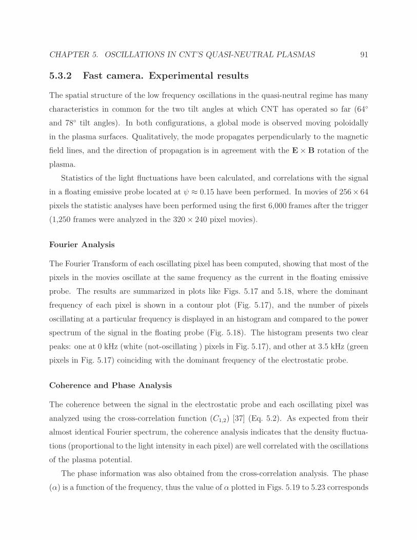
CHAPTER 5. OSCILLATIONS IN CNT’S QUASI-NEUTRAL PLASMAS 91
5.3.2 Fast camera. Experimental results
The spatial structure of the low frequency oscillations in the quasi-neutral regime has many
characteristics in common for the two tilt angles at which CNT has operated so far (64
and 78 tilt angles). In both configurations, a global mode is observed moving poloidally
in the plasma surfaces. Qualitatively, the mode propagates perpendicularly to the magnetic
field lines, and the direction of propagation is in agreement with the E×B rotation of the
plasma.
Statistics of the light fluctuations have been calculated, and correlations with the signal
in a floating emissive probe located at ψ ≈ 0.15 have been performed. In movies of 256× 64
pixels the statistic analyses have been performed using the first 6,000 frames after the trigger
(1,250 frames were analyzed in the 320× 240 pixel movies).
Fourier Analysis
The Fourier Transform of each oscillating pixel has been computed, showing that most of the
pixels in the movies oscillate at the same frequency as the current in the floating emissive
probe. The results are summarized in plots like Figs. 5.17 and 5.18, where the dominant
frequency of each pixel is shown in a contour plot (Fig. 5.17), and the number of pixels
oscillating at a particular frequency is displayed in an histogram and compared to the power
spectrum of the signal in the floating probe (Fig. 5.18). The histogram presents two clear
peaks: one at 0 kHz (white (not-oscillating ) pixels in Fig. 5.17), and other at 3.5 kHz (green
pixels in Fig. 5.17) coinciding with the dominant frequency of the electrostatic probe.
Coherence and Phase Analysis
The coherence between the signal in the electrostatic probe and each oscillating pixel was
analyzed using the cross-correlation function (C1,2) [37] (Eq. 5.2). As expected from their
almost identical Fourier spectrum, the coherence analysis indicates that the density fluctua-
tions (proportional to the light intensity in each pixel) are well correlated with the oscillations
of the plasma potential.
The phase information was also obtained from the cross-correlation analysis. The phase
(α) is a function of the frequency, thus the value of α plotted in Figs. 5.19 to 5.23 corresponds

CHAPTER 5. OSCILLATIONS IN CNT’S QUASI-NEUTRAL PLASMAS 92
Figure 5.17: Contour plot of the dominant frequency at each pixel. Most of the pixels exhibit
the same color, indicating a uniform dominant frequency in the movie (white color indicates
the pixel does not oscillate). View from the “nw” side port. pn = 8 · 10−5 Torr of N2, B =
0.02 T, φe = −200 V, 64 configuration.
Figure 5.18: Histogram of the number of pixels oscillating at a particular frequency (red).
Power spectrum of the floating probe overlaid (blue dots). Same shot as in Fig. 5.17.

CHAPTER 5. OSCILLATIONS IN CNT’S QUASI-NEUTRAL PLASMAS 93
to the phase at the dominant frequency of the cross-correlation power spectrum. The phase
plots in this Section only contain the phase information of the pixels whose RMS was greater
than 10% of the average RMS of the oscillating pixels in a movie, thus avoiding the potentially
random phase of low amplitude oscillations.
Fourier Transform g(t)→FT→ G(ω)
Cross correlation C1,2(ω) ≡ G1G∗2
Phase α1,2(ω) ≡ arctan
(Im [C1,2(ω)]
Real [C1,2(ω)]
)(5.2)
Field alignment and mode number
64 configuration
Experiments in the 64 tilt angle configuration showed that the mode number of the
oscillations jumps when the B field strength is raised above 0.05 T. Low frequency oscillations
(experiments at B = 0.02 T) seem to have a low poloidal mode number (m = 1 or 2), as can
be seen in the phase plot of Fig. 5.19 or the ensemble movies of Fig. 5.25. If this observation
is confirmed, this would imply that the quasi-neutral mode also breaks parallel force balance,
even though the mechanism driving the instability in this regime is different from the ion
driven mode described in Chapter 4.
However, high frequency oscillations (experiments at B ≥ 0.05 T) exhibit higher poloidal
mode numbers (two regions with the same phase are identified in a small strip of the plasma
in Fig. 5.21). In order to capture these higher frequency oscillations, the sampling frequency
of the camera was raised up to 75,000 fps, which reduced significantly the size of the frames
and only a narrow strip in the thick cross-section of the torus could be recorded. For
comparison, a black rectangle is drawn in Fig. 5.20 showing the area recorded by the camera
in Fig. 5.21. The copper mesh 1 can be used to obtain a rough estimate of k⊥ (k⊥ ≈ 63 m−1
at the edge of the plasma). This estimate is consistent with a m = 5 to 9 mode (resonant
with the rational magnetic surfaces in this configuration 2), suggesting that at high B field
1The size of the openings of the mesh is 8 mm.2The rotational transform varies from ι = 0.12 (on axis) to ι = 0.23 (at the plasma edge) in the 64
configuration

CHAPTER 5. OSCILLATIONS IN CNT’S QUASI-NEUTRAL PLASMAS 94
Figure 5.19: Contour plot of the phase at the dominant frequency of the cross-power spec-
trum (4549 Hz). View from the top view port. White color indicates that the amplitude of
the light oscillations in that pixel is small (the RMS of the oscillations in a pixel is lower
than 10% of the average RMS of the oscillating pixels in the movie). pn = 5 · 10−5 Torr of
N2, B = 0.02 T, φe = −200 V, 64 tilt angle.
strengths the mode can exist without breaking parallel force balance.
78 configuration
In the fast imaging experiments conducted for the 78 tilt angle configuration the visible
traces of the field lines were recorded and overlaid with the phase plots. These plots can be
used to obtain valuable information on the alignment of the oscillations with the field lines
and the mode number. Since the stabilization along the field lines occurs at least 20 times
faster than these oscillations, the phase of the oscillations is almost perfectly aligned with the
magnetic field lines (Fig. 5.22). The top view shown in Fig. 5.23 looks perpendicularly at the
thick poloidal cross section of the plasma. Two regions with the same phase can be clearly
identified in this phase plot, indicating that the poloidal mode number of the oscillations
seems to be m = 2. However, when these phase plots are analyzed, we have to take into
account that the camera is recording the light intensity integrated across the torus.
The simulation of the integral light intensity generated by modes rotating in the torus
is essential for a correct interpretation of the mode number. Therefore, the propagation of

CHAPTER 5. OSCILLATIONS IN CNT’S QUASI-NEUTRAL PLASMAS 95
Figure 5.20: Contour plot of the phase at the dominant frequency of the cross-power spec-
trum (4472 Hz). View from the “nw” side port. White color indicates that the amplitude
of the light oscillations in that pixel is small. A black rectangle is drawn showing the area
recorded by the camera in Fig. 5.21. pn = 5 · 10−5 Torr of N2, B = 0.02 T, φe = −200 V,
64 tilt angle.
Figure 5.21: Contour plot of the phase at the dominant frequency of the cross-power spec-
trum (8452 Hz). pn = 8 · 10−5 Torr of N2, B = 0.05 T, φe = −200 V, 64 tilt angle.

CHAPTER 5. OSCILLATIONS IN CNT’S QUASI-NEUTRAL PLASMAS 96
Figure 5.22: Contour plot of the phase at the dominant frequency of the cross-power spec-
trum (2795 Hz). View from the “nw” side port. The solid black lines correspond to the
trace of a field line in the magnetic surface where the electrons are emitted (the dashed lines
are the error bars). White color indicates that the amplitude of the light oscillations in that
pixel is small. pn = 5 · 10−5 Torr of N2, B = 0.04 T, φe = −200 V, 78 tilt angle.
field aligned m = 1, 2, 3 and 4 modes was simulated in a half CNT torus (details on these
simulations are provided on Appendix A). Comparing the experimentally obtained phase
plot (Fig. 5.23) with the phase plots of the simulated modes (Fig. 5.24), the structure of
the observed oscillations is closer to the simulated m = 3 mode. The 78 coil configuration
presents an almost flat iota profile close to ι = 1/3 [41], thus a poloidal m = 3 mode resonates
with the rational magnetic surfaces in this configuration.
Although the plasma potential is almost identical for both tilt angles in the quasi-neutral
regime (Fig. 3.13), the measured frequencies in the 78 configuration are lower compared to
the 64 tilt angle and cannot be increased too much by raising the magnetic field strength (2-5
kHz in the 78 tilt angle, while the frequency could be varied between 2 and 18 kHz in the 64
configuration). This provides additional evidence to the fact that quasi-neutral oscillations
jump to a higher mode number at stronger B fields in the 64 conf. The quasi-neutral
oscillations in the 78 configuration present a resonant m = 3 mode number independently

CHAPTER 5. OSCILLATIONS IN CNT’S QUASI-NEUTRAL PLASMAS 97
Figure 5.23: Contour plot of the phase at the dominant frequency of the cross-power spec-
trum (5031 Hz). View from the top window of the chamber. The solid black lines correspond
to the trace of a field line in the magnetic surface where the electrons are emitted (the dashed
lines are the error bars). White color indicates that the amplitude of the light oscillations in
that pixel is small. pn = 5 · 10−5 Torr of N2, B = 0.08 T, φe = −200 V, 78 tilt angle.

CHAPTER 5. OSCILLATIONS IN CNT’S QUASI-NEUTRAL PLASMAS 98
Figure 5.24: Phase plot of the simulated m = 1, 2, 3 and 4 modes. These graphs simulate the
visualization from the top window of the chamber. The solid black lines correspond to the
trace of a field line in the magnetic surface where the electrons are emitted. 78 tilt angle.
White color indicates that the amplitude of the light oscillations in that pixel is small.

CHAPTER 5. OSCILLATIONS IN CNT’S QUASI-NEUTRAL PLASMAS 99
of the B field strength, whereas in the 64 tilt angle the mode only seems to resonate with
the rational magnetic surfaces at strong B fields. Since the lowest poloidal mode numbers of
the resonant surfaces in the 64 configuration are m = 5 to m = 9, the measured frequency
is higher than in the 78 conf.
Ensemble movies
Efforts have also been devoted to relate movies from the top and the “nw” side ports using
a floating probe located at ψ ≈ 0.15 as the time reference. Particularly, the time reference is
chosen to be the phase of the mode that dominates the vast majority of the cross correlations
between the pixels of a movie and the signal in the electrostatic probe. In order to improve
the synchronization between the fast camera and the DAQ, a single acquisition card recorded
the oscillations in the floating probe and controlled the trigger sent to the fast camera. Since
the sampling frequency of the probe and the fast camera was different, the datasets had
to be resampled and interpolated at a common frequency arbitrary 10 times higher than
the dominant mode of the cross-power spectrums (10 phase bins per cycle of the dominant
mode). Then, the ensemble average of the signal at each phase bin (Fi) was computed for
the probe and for every pixel as:
Fi =1
M/10
M/10∑j=1
fi,j (5.3)
where, M is the total number of samples and fi,j are the samples of the dataset already
sorted in 10 different i bins.
The results are presented in movies like Fig. 5.25. In the top left corner we can see the
ensemble movie of the oscillations in the plasma from the top view port. Below we have the
corresponding ensemble signal of the floating probe in the same shot. An ensemble movie
taken from the “nw” side view port at the same experimental conditions can be seen in the
top right corner, with its corresponding ensemble signal of the electrostatic probe below.
To improve the visualization of the movies, the DC level of the light intensity has been
subtracted, and the 8-bit greyscale of the camera has been replaced by a blue (minimum
light intensity) to red (maximum light intensity) scale. The view of the plasma is partially
obstructed by the copper mesh and other objects in these movies, so some pixels do not

CHAPTER 5. OSCILLATIONS IN CNT’S QUASI-NEUTRAL PLASMAS 100
Figure 5.25: Two views of the plasma taken with one camera. Top and
side view are synchronized with the signal of the electrostatic probe. URL:
http://hdl.handle.net/10022/AC:P:10261.

CHAPTER 5. OSCILLATIONS IN CNT’S QUASI-NEUTRAL PLASMAS 101
oscillate and are colored in white. Although both movies were taken at the same experimental
conditions, the frequency of the dominant mode in the two shots is not identical (4.7 kHz
in the left shot, and 3.9 kHz in the right shot), and thus the time scale in the left and the
right hand movies is not exactly the same. Nevertheless, the aim of these visualizations is
successfully fulfilled, since they are intended to synchronize the oscillations in the plasma
from different view ports taking the phase of the floating probe as the reference.
Experiments at reversed polarity
The frequency of the oscillations in the quasi-neutral regime scales linearly with the plasma
potential, and grows with the φp/B ratio. The analysis of the fast camera movies shows that
the mode is almost perfectly aligned with the magnetic field lines, propagates perpendicularly
to the field lines, and the direction of propagation is in agreement with the E×B rotation of
the plasma. Everything seems to indicate that theE×B drift is convecting these oscillations,
but it remained to be studied how the direction of the magnetic field affected the rotation
of the mode. Therefore, the polarity of the coils was switched, consequently reversing the
direction of the magnetic field and the E×B drift while the magnetic surfaces remained
unchanged.
The top window of the chamber looks perpendicularly at the thick poloidal cross section
of the plasma. Movies recorded from this view port provide an excellent evidence of how
changing the direction of the magnetic field involves reversing the rotation of the mode, thus
confirming the role of the E×B drift. The movies in Fig. 5.26 are ensemble movies of the
oscillations, but the reversal of the direction of rotation when the polarity of the coils is
flipped can also be observed in the raw data movies.
5.3.3 Capacitive probes
The fast camera provides much better spatial resolution for the characterization of the quasi-
neutral mode, but the set of capacitive probes shown in Fig. 2.2 was also used to investigate
the spatial structure of the mode in the 78 configuration. Fig. 5.27 plots the measured
phase differences of the mode in each poloidal capacitive probe relative to TP 3 using the
same procedure described for the ion-resonant mode in electron-rich plasmas (section 4.3).

CHAPTER 5. OSCILLATIONS IN CNT’S QUASI-NEUTRAL PLASMAS 102
Usual polarity Reversed polarity
Figure 5.26: Ensemble movies from the top window.
Left: At the usual polarity the mode propagates counterclockwise. URL:
http://hdl.handle.net/10022/AC:P:10262.
Right: Whereas at reversed polarity the mode propagates clockwise. URL:
http://hdl.handle.net/10022/AC:P:10263.
The quasi-neutral oscillations propagate in the direction of the E×B rotation of the plasma,
and the measured phase shifts indicate that the poloidal structure of the mode is m = 3.
Similar results were obtained for all the experiments conducted at B ≤ 0.04 T. For B ≥ 0.05
T the Fourier spectrum of the oscillations present broader peaks at the edge of the plasma
(Fig. 5.9) and it was harder to study the phase shift of the mode.
Hence, agreement between the results obtained with the fast camera and the capacitive
probes is generally very good.
5.3.4 Discussion
The set of fast imaging experiments exploring the spatial structure of the quasi-neutral
oscillations show that this mode presents many characteristics in common for the two tilt
angles studied so far in CNT. In both configurations, a global mode is detected moving
poloidally in the plasma surfaces, the mode propagates perpendicularly to the magnetic field
lines (k ·B ≈ 0), and the direction of propagation is in agreement with the E×B drift. But

CHAPTER 5. OSCILLATIONS IN CNT’S QUASI-NEUTRAL PLASMAS 103
Figure 5.27: Measured phase shift of the quasi-neutral oscillations detected on the poloidal
capacitive probes. The phase on probe TP 3 is used as the reference. pn = 2 · 10−5 Torr of
N2, φe = −200 V, B = 0.02 T, 78 configuration.
also significant differences have been identified between the two configurations.
The experiments in the 78 configuration provide enough evidence to conclude that the
low frequency mode of our quasi-neutral plasmas is a flute instability, almost perfectly aligned
with the magnetic field lines and has a m = 3 mode number (resonant with rational magnetic
surfaces). This poloidal m = 3 structure was determined comparing the phase plots of the
oscillations recorded from the top view port (Fig. 5.23) with simulations of field aligned m
= 1 to m = 4 modes in the torus (Fig. 5.24), and also from the results obtained with a set
of capacitive probes at the edge of the plasma (Fig. 5.27).
The rotational transform in the 64 tilt angle configuration varies from ι = 0.12 to
ι = 0.23, i.e, the lowest poloidal mode numbers of the resonant surfaces in this configuration
are m = 5 to m = 9. For this tilt angle, the quasi-neutral oscillations seem to exhibit a low
poloidal mode number (clearly, m < 5) at low B field strengths (B = 0.02 T), suggesting
that the parallel force balance might be broken (as observed in the ion driven instability
of CNT’s electron-rich plasmas, although the physics causing the unstable fluctuations here
are different). When the magnetic field is raised above 0.05 T the poloidal structure of the

CHAPTER 5. OSCILLATIONS IN CNT’S QUASI-NEUTRAL PLASMAS 104
oscillations jumps to a higher mode number. This is clearly observed in the movies and
the phase plots (Fig. 5.21), but also in the measured frequency of the mode (for almost
identically potentials in the 64 and 78 tilt angle, the measured frequency is always higher
for the 64 conf). The estimate of k⊥ ≈ 63 m−1 and the measured frequency of the mode
suggests that at strong B fields the mode might be resonant with rational magnetic surfaces
in the 64 configuration, allowing this perturbation to exist without breaking parallel force
balance.
5.4 Summary and Discussion
Quasi-neutral plasmas (η < 10−5) have been systematically studied for the first time in
CNT. In this regime the plasma is completely decoupled from the emitter bias voltage,
and develops spontaneous single-mode low frequency oscillations (1 - 20 kHz). The plasma
presents slightly negative plasma potentials (0 < φp/φe < 0.1), which are mainly determined
by the magnetic field strength (the measured φp is more negative at higher magnetic field
strengths). The electron temperature in the core of the plasma (ψ ≈ 0.15) ranges between
30 and 45 eV, but does not have a clear relationship with the B field strength. CNT quasi-
neutral plasmas are also characterized by centrally peaked density profiles, with average
densities of ne ≈ 1015m−3. The Debye length in this regime is typically λD 1mm, which
is more than one order of magnitude smaller than λD in pure-electron plasmas [43].
The measured frequency of the quasi-neutral fluctuations has a negligible dependence on
η, and grows with the |φp/B| ratio. However, it does not present a clear linear scaling with
E/B (Fig. 5.6). The investigation on the spatial structure of the mode shows that detected
instability is a global mode almost perfectly aligned with the magnetic field lines, and prop-
agates in the direction of the E × B rotation of the plasma. The spatial structure of the
oscillations was studied in detail in the 78 configuration with two independent diagnostics
(a high speed camera and a set of capacitive probes) providing strong evidence to conclude
that the mode has a m = 3 poloidal structure (resonant with rational magnetic surfaces).
Low frequency instabilities in low-β plasmas have being traditionally classified according
to their drive mechanism into: Drift waves, Kelvin-Helmholtz, and Rayleigh-Taylor insta-
bilities [38]. The frequency of the oscillations is identical in the core of the plasma and

CHAPTER 5. OSCILLATIONS IN CNT’S QUASI-NEUTRAL PLASMAS 105
at different radial locations across the plasma (Fig. 5.8). Therefore, no velocity shear is
observed, which confirms that the detected instability is a global mode, and eliminates the
possibility of having a Kelvin-Helmholtz instability.
The plasma oscillations were measured simultaneously in a floating emissive probe and
an ion saturation probe to study the local phase shift between n and φ and discern the
nature of CNT quasi-neutral fluctuations. The analysis presented in Section 5.2.5 studies
the influence of the variation of Te and the growth of the sheath in the oscillations of the
current collected by the ion probe. The fluctuations in Iprobe are mainly caused by oscillations
of n (and not Te), and it is observed that the local phase shift between n and φ is 34± 57.
This confirms that the instability is not driven by the velocity shear (characterized by large
phase differences between n and φ). Although the measurements slightly favor drift waves,
the experimental uncertainties in the determination of the local phase shift are too large to
enable us to discriminate between drift waves and a Rayleigh-Taylor instability.
The drift wave frequency is ω∗ = k⊥ρscs/Ln, where ρs = cs/ωi, cs is the ion acoustic speed
cs =√Te/mi, and Ln is the density scale length. The measured frequency (ω) of a drift
wave is normally Doppler shifted by the E ×B rotation of the plasma, ω = ωE×B ± ω∗ [64].
Rayleigh-Taylor instabilities, however, propagate at the E ×B velocity of the plasma [38].
For a φe = −200 V quasi-neutral plasma at B = 0.04 T in the 78 configuration, the
measured plasma potential is typically φp ≈ −7 V (Fig. 3.13), so f = mfE×B ≈ 3.7 kHz,
which is consistent with the measured frequency of CNT quasi-neutral mode. For a plasma
of the same characteristics, Te ranges between 30 and 45 eV (Fig. 5.1), thus f = mf∗ ≈15 − 24 kHz, which is significantly higher than the measured frequency of the instability at
B = 0.04 T. Since φp < 0 in CNT, electron drift wave fluctuations will add to the E × Brotation of the plasma.
Table 5.1 compares features of CNT’s quasi-neutral wave with the predicted values for
drift waves and Rayleigh-Taylor instabilities [38]. It is difficult to discern between both types
of instabilities based on the available measurements, however the mode seems to propagate
closer to ωE×B, and a rough estimate of the growth rates (γ) of the instabilities shows that
γRT ∼ cs/√LpRc is faster than γDW ∼ ω∗ (assuming the pressure scale length, Lp, as
the minor radius of the torus, and the radius of curvature, Rc, as the major radius). Hence,
CNT’s instability might be described as density blobs expanding where the pressure gradient

CHAPTER 5. OSCILLATIONS IN CNT’S QUASI-NEUTRAL PLASMAS 106
Table 5.1: Comparison of experimental results and theoretical predictions. The predicted
features for drift waves and Rayleigh-Taylor instabilities are based on the criteria derived by
Jassby [38], unless otherwise stated.
cs is the ion acoustic speed, cs =√Te/mi. Lp is the pressure scale length, L−1
p = |∇p|/p.Rc is the radius of curvature.
CNT quasi-neutral
oscillations Drift waves Rayleigh-Taylor
frequency ∼ ωE×B ωE×B ± ω∗ ωE×B
local n - φ phase shift 34 ± 57 0 to 45 45 to 90
k|| ∼ 0 > 0 0
mode number, m 3 no restriction 1 or 2 a∣∣∣eφ/Te∣∣∣ / |n/n| usually < 1 1 1
growth rate, γ - ∼ ω∗ [33, 64] ∼ cs/√LpRc [27]
aIn the absence of magnetic surfaces

CHAPTER 5. OSCILLATIONS IN CNT’S QUASI-NEUTRAL PLASMAS 107
is anti-parallel to the magnetic field curvature, like the flute instability observed in magnetic
mirrors [27, 69]. CNT, indeed, can be seen as two linked magnetic mirrors. Rayleigh-Taylor
and drift instabilities might also coexist and couple in CNT. The study of the transition
from a regime dominated by drift waves to a regime dominated by interchange modes has
been an active area of research in other experiments [14, 32, 64, 77], and can be of interest
for future investigations in CNT.
The oscillations detected in the quasi-neutral regime are a global flute instability (k ·B ≈0) convected by the E ×B flow, and probably driven by the bad curvature in the outboard
side of a torus (i.e., Rayleigh-Taylor / interchange instability), or the coupling of both drift
and interchange modes.
The presence of magnetic shear has a stabilizing effect on these instabilities [27, 33] and
should have been manifested comparing the behavior of the quasi-neutral oscillations in the
78 (essentially shear-less) and the 64 (reversed shear) configurations. However, the oscilla-
tions behave very similarly under completely different shear configurations (Fig. 5.7). These
results therefore challenge our theoretical understanding of magnetic shear stabilization.

Chapter 6
Conclusions
The study of partially neutralized plasmas lies between two traditionally separated fields
in plasma physics: non-neutral plasma physics (focused on the study of single component
plasmas), and quasi-neutral plasmas. The physics of partially neutralized plasmas remains
largely unexplored, partly because of the difficulty of confining such plasmas. Penning-
Malmberg and pure toroidal traps have been successfully used to study single component
plasmas, but cannot confine partly neutralized or quasi-neutral plasmas. Tokamaks, on
the other hand, require large internal currents for confinement, which cannot be driven in
the low densities typical of non-neutral plasmas [8, 13]. However, stellarators can confine
plasmas of any degree of neutralization (from pure electron to quasi-neutral) without the
need for a plasma current. The studies conducted for this thesis in the CNT stellarator
represent the first experimental characterization of plasmas of arbitrary neutrality. This
Chapter summarizes and discusses the results reported in this thesis.
The degree of neutralization of the plasma can be parameterized through the quantity
η ≡ |ne − Zni|/|ne + Zni|. CNT can vary continuously η from pure electron (η = 1) to
quasi-neutral (η 1) by adjusting the neutral pressure in the chamber, which controls the
steady state balance between the volumetric ionization of neutrals and the recombination of
ions in the ceramic rods. CNT can operate steadily at any given value of η between 10−5
and 1.
Pure electron plasmas in CNT are in macroscopically stable equilibria [43], and are
characterized by a close match between the local plasma potential and the emitter filament
108

CHAPTER 6. CONCLUSIONS 109
bias voltage. The emitter bias dictates the plasma potential on the magnetic axis, which
determines the total electron content through Poisson’s equation. However, the accumulation
of ions alters very significantly the equilibrium of electron-rich plasmas. As η evolves from
pure electron to quasi-neutral, the plasma potential decouples from the emitter bias, and
spontaneous fluctuations appear.
The presence of a second ceramic rod halves the ion content in the plasma for a given neu-
tral pressure [49]. The neutral pressure threshold for the decoupling of the plasma potential,
and the appearance of fluctuations, is doubled when an additional ceramic rod is inserted in
the plasma (which corresponds approximately to the same ion content). This confirms that
the accumulation of ions (and not the presence of neutrals or an emission limit) is responsi-
ble for the separation of the plasma potential and the development of unstable oscillations.
CNT plasmas develop unstable fluctuations for η < 0.8, and the abrupt separation of the
plasma potential profiles from the emitter voltage occurs when a threshold of η ≈ 10−3 is
exceeded.
As a result of the decoupling of the plasma potential from the emitter bias, the emitted
electrons are accelerated, and become hotter. Te in a typical CNT pure electron plasma
ranges between 2 and 7 eV in the core of the plasma, while quasi-neutral plasmas (η < 10−5)
exhibit Te between 30 and 45 eV.
Ions, on the other hand, cool down as the plasma detaches from the emitter bias. As the
ions are drawn into the electron-rich plasma, part of the potential drop across the plasma is
transferred to the ions’ kinetic energy. Massive ions (such as N+2 ) are largely unmagnetized at
η ≈ 1, but when the plasma potential decouples (becomes less negative), the ion gyro-radius
(rLi) gets smaller than the minor radius of the torus, 〈a〉. For η < 10−5, rLi/〈a〉 < 1.
The fluctuations detected in plasmas of arbitrary neutrality confined in CNT can be
classified into three categories according to their behavior (single mode or multi-mode) and
their degree of neutrality: 1) single mode oscillations in electron-rich plasmas (0.01 < η <
0.8), 2) multiple mode fluctuations in electron-rich plasmas (10−4 < η < 0.1), and 3) single
mode oscillations in quasi-neutral plasmas (η < 10−5). The presence of magnetized ions
traveling close to the E × B drift is essential for the excitation of a single mode instability
in electron-rich plasmas. Otherwise, largely unmagnetized ions bounce chaotically in the
electron-rich plasma and multiple modes are excited. This thesis describes the single mode

CHAPTER 6. CONCLUSIONS 110
oscillations observed in partially neutralized and quasi-neutral plasmas.
Ion-driven fluctuations were predicted to be damped by the magnetic surfaces much faster
than the period of an oscillation [50, 59]. However, electron-rich plasmas (0.01 < η < 0.8)
confined on magnetic surfaces exhibit a single mode ion-driven oscillation at high B field
strengths (B > 0.04 T) or when light ion species (He+) are present. The instability observed
in CNT has characteristics in common with the ion resonant mode previously studied in
Penning-Malmberg [5,63], and pure toroidal traps [75,76]. The frequency of CNT’s ion-driven
mode ranges between 20 and 100 kHz, and scales close to linearly with φp/B, suggesting a
relation to the E×B flow of the plasma. However, the measured frequency of the mode also
presents a small dependence on the ion species introduced, which implies that the mode is not
a purely E×B rotation of the plasma. The density and potential fluctuations driven by the
ion-resonant instability seem to be in phase, which is in agreement with the predictions for
small oscillatory perturbations (|eφ|/Te < 1) in an electron-rich plasma confined on magnetic
surfaces.
The spatial structure and the direction of propagation of CNT’s ion-driven mode were
investigated with a set of capacitive probes. The instability is a global mode propagating in
the E ×B direction. The ion-driven mode presents a m = 1 poloidal mode number for both
magnetic configurations studied so far in CNT (64 [50] and 78 tilt angle, reported in this
thesis). This implies that even low order rational magnetic surfaces cannot stabilize the ion
resonant mode, and the instability breaks the parallel force balance. The mechanism leading
to the violation of parallel force balance in the magnetic surfaces is not totally understood
at this point, but might be related to the presence of an anisotropic pressure tensor which
modifies the plasma force balance equation in a way that an isotropic pressure cannot.
The ion-driven mode in a stellarator is predicted to have a toroidal mode number n > 0
in order to conserve the poloidal magnetic flux (even if the parallel force balance is broken).
However, the toroidal structure of the ion-driven mode has now been determined to be n
= 0. This implies that the poloidal flux is not conserved in a close tube of plasma moving
with the ion-driven mode. The explanation for this behavior probably lies in the presence
of a non-scalar pressure (due to the large fraction of trapped particles in CNT), which
invalidates the ideal MHD approximation of Ohm’s law in CNT (fundamental assumption
for the conservation of magnetic flux in an ideal plasma).

CHAPTER 6. CONCLUSIONS 111
Quasi-neutral plasmas (η < 10−5) in CNT are characterized by much weaker electric
fields (|eφp| < Te), and the presence of spontaneous single mode low frequency oscillations
(1 - 20 kHz). The measured frequency of the mode grows with the |φp/B| ratio, but does
not present a clear linear scaling with E/B.
A high speed camera and a set of capacitive probes were used to study the spatial struc-
ture of the quasi-neutral oscillations, showing very good agreement between both diagnostics.
The detected instability is a global mode propagating in the E ×B direction of the plasma
and almost perfectly aligned with the magnetic field lines. The oscillations were determined
to have a m = 3 poloidal mode number, which is resonant with the almost flat ι ≈ 1/3 profile
of the 78 configuration.
The ion-driven instability detected in CNT’s electron-rich plasmas is stable in the quasi-
neutral regime [18, 19]. It is also clear that the driving mechanism behind CNT’s quasi-
neutral oscillations cannot be a Kelvin-Helmholtz instability since no velocity shear was
observed, and the local phase difference between density and potential fluctuations is small.
Although the measured n - φ phase shift slightly favors drift waves, the large uncertainty in
the determination of the phase difference does not allow to discriminate between drift waves
and a Rayleigh-Taylor instability by simply measuring this quantity.
Both drift waves and Rayleigh-Taylor instabilities are potential candidates for driving
CNT’s quasi-neutral mode. Nevertheless, the mode seems to propagate close to ωE×B (char-
acteristic of R-T instabilities), and the growth rate γRT appears to be faster than γDW .
Therefore, CNT’s global flute instabilities are likely to be density blobs expanding due to
the bad curvature in the outboard side of a torus, or perhaps, a combination of bad curvature
and drift instabilities.

Chapter 7
Possible Future Studies
This thesis describes the first experimental observations of plasmas of arbitrary neutrality,
varying η continuously from pure electron to quasi-neutral. Many questions remain to be
answered to understand the physics of partially neutralized plasmas. Some ideas for future
research in this largely uncharted territory for plasma physics are summarized below:
• Understanding how CNT’s ion-driven instability breaks parallel force bal-
ance and the conservation of the poloidal magnetic flux. The measured m =
1, n = 0 spatial structure of CNT’s ion resonant mode suggests that the instability
violates parallel force balance and the conservation of the poloidal magnetic flux in the
stellarator. Preliminary interpretations explain the violation of parallel force balance
as a consequence of the large fraction of trapped particles which remain in a locally
perturbed region, and do not stream along the field lines, allowing the instability to
exist breaking parallel force balance [50]. This thesis also discusses how the presence
of an anisotropic pressure tensor modifies the plasma force balance equation, which
invalidates the ideal MHD Ohm’s law, and might explain the apparent breaking of
parallel force balance, and the violation of the conservation of poloidal magnetic flux.
However, further studies are needed to confirm these hypotheses.
• Multi-mode / broad band oscillations in partially neutralized plasmas. This
thesis mainly investigates the single mode oscillations detected in partially neutralized
and quasi-neutral plasmas. However, the presence of broadband fluctuations are also
112

CHAPTER 7. POSSIBLE FUTURE STUDIES 113
very characteristic of partially neutralized plasmas.
Multiple peak oscillations occur for degrees of non-neutrality between η = 0.01 and
0.1 when the ions are largely unmagnetized and bounce chaotically in the electron rich
plasma. The multiple modes excited present frequencies below 100 kHz, which is in
the range of the E ×B rotation and the ion bounce frequency in the plasma, but it is
unclear what is the driving mechanism of these modes.
For 10−4 < η < 0.01 the maximum amplitude and broadest power spectra of the
oscillations are always observed. The Fourier spectrum in this regime is typically
dominated by a broad peak between 100 and 200 kHz, but lower frequency modes
are also detected whose frequency decreases as η approaches quasi-neutrality. Plasmas
with more magnetized ions present narrower power spectra.
Further experimental and theoretical studies have to be conducted for a comprehensive
understanding of multi-mode oscillations in partially neutralized plasmas.
• Jumps between equilibrium states in partially neutralized plasmas. For de-
grees of neutralization close to η ≈ 10−3 the plasma decouples rather abruptly from the
emitter bias voltage and the emission current grows significantly. Sometimes during
the same shot the plasma switches back and forth between a stable equilibrium state
(plasma potential close to the emitter bias and low emission currents) and a metastable
state (in which the plasma is decoupled from the emitter bias and the emission current
is much higher). Since the separation of the plasma potential from the emitter bias
is caused by the accumulation of ions (Section 3.3.2), the jumps between states in
partially neutralized plasmas could be explained in terms of a process that enhances
ionization.
Preliminary observations are described in Section 4.4.2, but future research is needed
to understand these jumps between equilibrium states. The characterization of the
equilibrium states before and after the decoupling from emitter bias voltage will be of
particular interest.
• Measurements of the ion temperature in CNT. An interesting study to be
conducted in order to understand the behavior of partially neutralized plasmas would

CHAPTER 7. POSSIBLE FUTURE STUDIES 114
be the measurement of the ion distribution function. Ions are generated in our plasmas
by electron-neutral collisions and are drawn electrostatically into the plasma without
collisions, therefore the distribution function of ions is predicted to be non-Maxwellian.
A gridded energy analyzer [34] can be used to measure the ion distribution function,
which has not been studied experimentally yet in CNT.
• A more detailed investigation on the drift / interchange nature of CNT’s
quasi-neutral mode. It has been difficult to discriminate the driving mechanism of
CNT’s quasi-neutral oscillations between drift and Rayleigh-Taylor instabilities. Both
types of instabilities might also couple in CNT. Further investigations are essential for
a deeper understanding of CNT’s flute instability, and can connect research in CNT
with the study of the controlled transition from regimes dominated by drift waves to
regimes showing interchange character [14, 32, 64, 77].

Bibliography
[1] K. Avinash. On toroidal equilibrium of non-neutral plasma. Phys. Fluids B, 3(12),
1991.
[2] J.W. Berkery, Q.R. Marksteiner, T. Sunn Pedersen, J.P. Kremer, and R.G. Lefran-
cois. Ion accumulation in a pure electron plasma confined on magnetic surfaces. Phys.
Plasmas, 14:084505, 2007.
[3] J.W. Berkery, T. Sunn Pedersen, J.P. Kremer, Q.R. Marksteiner, R.G. Lefrancois, M.S.
Hahn, and P.W. Brenner. Confinement of pure electron plasmas in the Columbia Non-
neutral Torus. Phys. Plasmas, 14(6), 2007.
[4] J.W. Berkery, T. Sunn Pedersen, and L. Sampedro. A retractable electron emitter for
the creation of unperturbed pure electron plasmas. Rev. Sci. Instrum., 78(1):013504,
2007.
[5] G Bettega, F Cavaliere, M Cavenago, A Illiberi, R Pozzoli, and M Rom. Experimental
investigation of the ion resonance instability in a trapped electron plasma. Plasma
Physics and Controlled Fusion, 47(10):1697, 2005.
[6] A. H. Boozer. Private communication.
[7] Allen H. Boozer. What is a stellarator? volume 5, pages 1647–1655. AIP, 1998.
[8] Allen H. Boozer. Density limit for electron plasmas confined by magnetic surfaces. Phys.
Plasmas, 12(10):104502, 2005.
[9] Allen H. Boozer. Physics of magnetically confined plasmas. Rev. Mod. Phys.,
76(4):1071–1141, Jan 2005.
115

BIBLIOGRAPHY 116
[10] P. Brenner, T. S. Pedersen, X. Sarasola, and M. Hahn. Confinement studies in the
Columbia Non-neutral Torus. volume 50, pages 678–682. WILEY-VCH Verlag, 2010.
[11] P.W. Brenner. Confinement of Non-Neutral Plasmas in Stellarator Magnetic Surfaces.
PhD thesis, Columbia University, 2011.
[12] P.W. Brenner, T.S. Pedersen, J.W. Berkery, Q.R. Marksteiner, and M.S. Hahn. Mag-
netic surface visualizations in the Columbia Non-neutral Torus. Plasma Science, IEEE
Transactions on, 36(4):1108–1109, Aug. 2008.
[13] Leon Brillouin. A theorem of Larmor and its importance for electrons in magnetic fields.
Phys. Rev., 67(7-8):260–266, Apr 1945.
[14] F. Brochard, E. Gravier, and G. Bonhomme. Transition from flute modes to drift waves
in a magnetized plasma column. Physics of Plasmas, 12(6):062104, 2005.
[15] D. Carralero et al. Turbulence studies by fast camera imaging experiments in the TJ-II
stellarator. Journal of Nuclear Materials, 390-391:457 – 460, 2009.
[16] N. D’Angelo and S. v. Goeler. Investigation of the Kelvin-Helmholtz instability in a
Cesium plasma. Physics of Fluids, 9(2):309–313, 1966.
[17] J. D. Daugherty, J. E. Eninger, and G. S. Janes. Experiments on the injection and
containment of electron clouds in a toroidal apparatus. Phys. Fluids, 12(12):2677, 1969.
[18] R. C. Davidson. Physics of Nonneutral Plasmas. Imperial College Press and World
Scientific Publishing, London, UK, Second edition, 2001.
[19] R. C. Davidson and Hwan sup Uhm. Influence of finite ion Larmor radius effects on the
ion resonance instability in a nonneutral plasma column. Physics of Fluids, 21(1):60–71,
1978.
[20] Benoit Durand de Gevigney. Theoretical and Numerical Investigation of Transport in
the Columbia Non-neutral Torus. PhD thesis, Columbia University, 2010.

BIBLIOGRAPHY 117
[21] Benoit Durand de Gevigney, Thomas Sunn Pedersen, and Allen H. Boozer. Numerical
investigation of electron trajectories in the Columbia Non-neutral Torus. Physics of
Plasmas, 16(12):122502, 2009.
[22] T. Estrada et al. Electron internal transport barrier formation and dynamics in the
plasma core of the TJ-II stellarator. Plasma Phys. Control. Fusion, 46:277, 2004.
[23] J. Fajans. Non-neutral plasma equilibria, trapping, separatrices, and separatrix crossing
in magnetic mirrors. Physics of Plasmas, 10(5):1209–1214, 2003.
[24] K. S. Fine, C. F. Driscoll, and J. H. Malmberg. Measurements of a nonlinear diocotron
mode in pure electron plasmas. Phys. Rev. Lett., 63(20):2232–2235, Nov 1989.
[25] D.T. Garnier, A.K. Hansen, J. Kesner, M.E. Mauel, P.C. Michael, J.V. Minervini,
A. Radovinsky, A. Zhukovsky, A. Boxer, J.L. Ellsworth, I. Karim, and E.E. Ortiz.
Design and initial operation of the LDX facility. Fusion Engineering and Design, 81(20-
22):2371 – 2380, 2006. Proceedings of the Fifteenth International Toki Conference on
Fusion and Advanced Technology - ITC-15 SI.
[26] J. C. Glowienka, W. C. Jennings, and R. L. Hickok. Experimental investigation of a
coherent flute instability using a heavy ion beam probe. Physics of Fluids, 31(9):2704–
2709, 1988.
[27] R.J. Goldston and P.H. Rutherford. Introduction to Plasma Physics. Taylor & Francis,
1995.
[28] M. Hahn, T. Sunn Pedersen, Q. Marksteiner, and J. W. Berkery. Confirmation of a large
density variation along the magnetic axis of the Columbia Non-neutral Torus. Phys.
Plasmas, 15:020701, 2008.
[29] Michael Hahn. Pure Electron Plasma Equilibrium and Transport Jumps in The
Columbia Non-neutral Torus. PhD thesis, Columbia University, 2009.
[30] Michael Hahn, Thomas Sunn Pedersen, Paul W. Brenner, and Quinn Marksteiner.
Confinement jumps in a non-neutral plasma. Phys. Plasmas, 16(2):022105, 2009.

BIBLIOGRAPHY 118
[31] T.C. Hender et al. Chapter 3: MHD stability, operational limits and disruptions. Nuclear
Fusion, 47(6):S128, 2007.
[32] B.-G. Hong, W. Horton, S. Hamaguchi, M. Wakatani, M. Yagi, and H. Sugama. Tran-
sition from resistive-g to ηi- driven turbulence in stellarator systems. Physics of Fluids
B: Plasma Physics, 3(7):1638–1643, 1991.
[33] W. Horton. Drift waves and transport. Rev. Mod. Phys., 71(3):735–778, Apr 1999.
[34] I. H. Hutchinson. Principles of Plasma Diagnostics. Cambridge University Press, second
edition, 2002.
[35] K. Ichiguchi, M. Wakatani, T. Unemura, T. Tatsuno, and B.A. Carreras. Improved
stability due to local pressure flattening in stellarators. Nuclear Fusion, 41(2):181,
2001.
[36] S. Ide and the JT-60 Team. Overview of JT-60U progress towards steady-state advanced
tokamak. Nuclear Fusion, 45(10):S48, 2005.
[37] Emmanuel C. Ifeachor and Barrie W. Jervis. Digital Signal Processing: A Practical
Approach. Prentice Hall, 2001.
[38] D. L. Jassby. Transverse velocity shear instabilities within a magnetically confined
plasma. Phys. Fluids, 15(9):1590–1604, 1972.
[39] W. Knauer. Diocotron instability in plasmas and gas discharges. Journal of Applied
Physics, 37(2):602–611, 1966.
[40] Shigeo Kondoh, Tomoya Tatsuno, and Zensho Yoshida. Stabilization effect of magnetic
shear on the diocotron instability. Phys. Plasmas, 8(6):2635–2640, 2001.
[41] J.P. Kremer. The Creation and First Studies of Electron Plasmas in the Columbia
Non-neutral Torus. PhD thesis, Columbia University, 2006.
[42] J.P. Kremer, T. Sunn Pedersen, Q. Marksteiner, and R.G. Lefrancois. Diagnosing pure-
electron plasmas with internal particle flux probes. Rev. Sci. Instrum., 78(1):013503,
2006.

BIBLIOGRAPHY 119
[43] J.P. Kremer, T. Sunn Pedersen, Q. Marksteiner, and R.G. Lefrancois. Experimental
confirmation of stable, small Debye length pure electron plasma equilibria in a stellara-
tor. Phys. Rev. Lett., 97, 2006.
[44] R.G. Lefrancois and T. Sunn Pedersen. Large density variation predicted along the
magnetic axis for cold electron plasmas in the Columbia Nonneutral Torus (CNT).
Phys. Plasmas, 13:120702, 2006.
[45] R.G. Lefrancois, T. Sunn Pedersen, A.H. Boozer, and J.P. Kremer. Numerical investi-
gation of three-dimensional single-species plasma equilibria on magnetic surfaces. Phys.
Plasmas, 12:072105, 2005.
[46] Jr. Lyman Spitzer. The stellarator concept. Phys. Fluids, 1(4):253–264, 1958.
[47] J. H. Malmberg and J. S. deGrassie. Properties of nonneutral plasmas. Phys. Rev. Lett.,
35:577–580, 1975.
[48] J. H. Malmberg and C. F. Driscoll. Long-time containment of a pure electron plasma.
Phys. Rev. Lett., 44(10):654–657, Mar 1980.
[49] Q.R. Marksteiner. Studies of Non-neutral Ion Electron Plasmas Confined on Magnetic
Surfaces. PhD thesis, Columbia University, 2008.
[50] Q.R. Marksteiner, T. Sunn Pedersen, J.W. Berkery, M.S. Hahn, J.M. Mendez, B. Du-
rand de Gevigney, and H. Himura. Observations of an ion driven instability in non-
neutral plasmas confined on magnetic surfaces. Phys. Rev. Lett., 100(6):065002, 2008.
[51] M.E. Mauel, H.H. Warren, and A. Hasegawa. An experiment to measure collisionless
radial transport of energetic electrons confined by a dipole magnetic field. Plasma
Science, IEEE Transactions on, 20(6):626 –630, December 1992.
[52] D.A. Maurer. Magnetic Island Dynamics Induced by Rotating Magnetic Perturbations
in Tokamak plasma. PhD thesis, Columbia University, 2000.
[53] S. Morimoto, N. Yanagi, M. Nakasuga, T. Obiki, A. Iiyoshi, and K. Uo. Measurements
of Pfirsch-Schluter current and pressure profile for the high density ECH plasmas in
Heliotron DR. Nuclear Fusion, 28(9):1491, 1988.

BIBLIOGRAPHY 120
[54] N. Nishino, T. Mizuuchi, et al. 2-D image diagnostic technique for edge turbulence
using fast cameras. Plasma and Fusion Research, 2:S1055–S1055, 2007.
[55] N. Ohno, A. Komori, M. Tanaka, and Y. Kawai. Instabilities associated with a negative
rf resistance in current-carrying ion sheaths. Physics of Fluids B: Plasma Physics,
3(1):228–235, 1991.
[56] T. M. O’Neil. A confinement theorem for nonneutral plasmas. Phys. Fluids, 23:2217,
1980.
[57] T. M. O’Neil and R. A. Smith. Stability theorem for a single species plasma in a toroidal
magnetic configuration. Phys. Plasmas, 8(2430), 1994.
[58] T. Sunn Pedersen. Numerical investigation of two-dimensional pure electron plasma
equilibria on magnetic surfaces. Phys. Plasmas, 10(2):334–338, 2003.
[59] T. Sunn Pedersen and A.H. Boozer. Confinement of noneutral plasmas on magnetic
surfaces. Phys. Rev. Lett., 88(20):205002, 2002.
[60] T. Sunn Pedersen, A.H. Boozer, J.P. Kremer, and R.G. Lefrancois. Confinement of
plasmas of arbitrary neutrality in a stellarator. Phys. Plasmas, 11(5):2377–2381, 2004.
[61] T. Sunn Pedersen, A.H. Boozer, J.P. Kremer, R.G. Lefrancois, W.T. Reiersen,
F. Dahlgreen, and N. Pomphrey. The Columbia Nonneutral Torus: A new experiment
to confine nonneutral and positron-electron plasmas in a stellarator. Fusion Science and
Technology, 46:200–208, 2004.
[62] T. Sunn Pedersen, J.P. Kremer, R.G. Lefrancois, Q. Marksteiner, N. Pomphrey, W.T.
Reiersen, F. Dahlgreen, and X. Sarasola. Construction and initial operation of the
Columbia Nonneutral Torus. Fusion Science and Technology, 50:372–381, 2006.
[63] A. J. Peurrung, J. Notte, and J. Fajans. Observation of the ion resonance instability.
Phys. Rev. Lett., 70(3):295–298, Jan 1993.
[64] F. M. Poli, P. Ricci, A. Fasoli, and M. Podesta. Transition from drift to interchange in-
stabilities in an open magnetic field line configuration. Physics of Plasmas, 15(3):032104,
2008.

BIBLIOGRAPHY 121
[65] G Prasad, D Bora, Y C Saxena, and G C Sethia. Study of low-frequency flute-type
coherent fluctuations in a toroidal plasma. Plasma Physics and Controlled Fusion,
37(4):387, 1995.
[66] J. Qin et al. Measurements of plasma beta in stellarators. Nuclear Fusion, 36(3):381,
1996.
[67] Robert J. Renka. Multivariate interpolation of large sets of scattered data. ACM Trans.
Math. Softw., 14:139–148, June 1988.
[68] B.W. Rice, K.H. Burrell, J.R. Ferron, C.M. Greenfield, G.L. Jackson, L.L. Lao, R.J. La
Haye, T.C. Luce, B.W. Stallard, E.J. Strait, E.J. Synakowski, T.S. Taylor, A.D. Turn-
bull, and M.R. Wade. Progress towards sustainment of advanced tokamak modes in
DIII-D. Nuclear Fusion, 39(11Y):1855, 1999.
[69] M. N. Rosenbluth and C. L. Longmire. Stability of plasmas confined by magnetic fields.
Annals of Physics, 1(2):120 – 140, 1957.
[70] H. Saitoh, Z. Yoshida, C. Nakashima, H. Himura, J. Morikawa, and M. Fukao. Confine-
ment of pure-electron plasmas in a toroidal magnetic-surface configuration. Phys. Rev.
Lett., 92(25):255005, 2004.
[71] H. Saitoh, Z. Yoshida, and S. Watanabe. Stable confinement of toroidal electron plasmas
in an internal conductor device prototype-ring trap. Phys. Plasmas, 12:092102, 2005.
[72] M. K. Vijaya Sankar, E. Eisner, A. Garofalo, D. Gates, T. H. Ivers, R. Kombargi,
M. E. Mauel, D. Maurer, D. Nadle, G. A. Navratil, and Q. Xiao. Initial high beta
operation of the HBT-EP tokamak. Journal of Fusion Energy, 12:303–310, 1993.
10.1007/BF01079674.
[73] M. Shimada et al. Chapter 1: Overview and summary. Nuclear Fusion, 47(6):S1, 2007.
[74] M. R. Stoneking, P. W. Fontana, R. L. Sampson, and D. J. Thuecks. Electron plasmas
in a ”partial” torus. Phys. Plasmas, 9(3):766, 2002.

BIBLIOGRAPHY 122
[75] M. R. Stoneking, M. A. Growdon, M. L. Milne, and R. T. Peterson. Millisecond con-
finement and observation of the m = 1 diocotron mode in a toroidal electron plasma.
AIP Conference Proceedings, 692(1):310–319, 2003.
[76] M.R. Stoneking, M.A. Growdon, M.L. Milne, and R.T. Peterson. Poloidal E × B drift
used as an effective rotational transform to achieve long confinement times in a toroidal
electron plasma. Phys. Rev. Lett., 92(9), 2004.
[77] Hideo Sugama, Masahiro Wakatani, and Akira Hasegawa. Study of resistive drift and
resistive interchange modes in a cylindrical plasma with magnetic shear. Physics of
Fluids, 31(6):1601–1608, 1988.
[78] A. Weller et al. Survey of magnetohydrodynamic instabilities in the advanced stellarator
wendelstein 7-as. Physics of Plasmas, 8(3):931–956, 2001.
[79] W. D. White, J. H. Malmberg, and C. F. Driscoll. Resistive-wall destabilization of
diocotron waves. Phys. Rev. Lett., 49(25):1822–1826, Dec 1982.
[80] M. Y. Ye and S. Takamura. Effect of space-charge limited emission on measurements
of plasma potential using emissive probes. Phys. Plasmas, 7(8):3457–3463, 2000.
[81] Puravi Zaveri, P. I. John, K. Avinash, and P. K. Kaw. Low-aspect-ratio toroidal equi-
libria of electron clouds. Phys. Rev. Lett., 68(22):3295, 1992.

Appendix A
Simulation of the mode number in
quasi-neutral plasmas
Movies simulating the propagation of field aligned m = 1, 2, 3 and 4 modes have been
produced to determine the mode number of the quasi-neutral oscillations. The only input
required for these simulations was the coordinates of the field lines in the magnetic surfaces,
which were obtained from the Field Line Follower code [41].
The Follower code takes small steps along magnetic field lines many times around the
torus, and returns the cylindrical coordinates of every step taken. For the simulations of
the mode number described in this Appendix, 5 irrational field lines producing good nested
magnetic surfaces between ψ ≈ 0.05 and ψ ≈ 0.5 were chosen (this ψ range presumably
corresponds to the surfaces that glow most in the experiments with the fast camera). Co-
ordinates from only one period of CNT’s torus (between ϕ = 0 and 180) were used for
simplicity, and also for flexibility (if the whole torus had been used, the resonant m = 3
mode would have been the only possible low mode aligned with the field lines). Each of the
5 field lines was split in as many segments as transitions the field line performed around the
torus. The poloidal angle of each field line segment was computed at the ϕ = 90 poloidal
cross section of the torus, and a “simulated light intensity” was assigned to each field line
segment taking into account its poloidal angle, and the simulated mode number.
The last main step in the simulation involves the interpolation of the light intensity
of the field lines in a regular grid. 3D interpolation methods like the Modified Shepard’s
123

APPENDIX A. SIMULATION OF THE MODE NUMBER 124
Figure A.1: Interpolated light intensity of a m = 2 mode in the mid horizontal plane.
Normalized x and y coordinates.
Method [67] failed to produce satisfactory results for the high number of field line coordinates
supplied. Since the aim of the simulation is the computation of the integrated light intensity
along the z axis, the torus was divided in 100 horizontal (z = constant) slices, and the
light intensity was interpolated in a 100 × 100 grid in each horizontal plane using the 2D
kriging interpolation method implemented in IDL . An example of the interpolated light
intensity of a m = 2 mode in a horizontal plane is provided in Fig. A.1. The only trivial
step that remains for the creation of a simulated movie frame is the summation along z of
the light intensity coming from all the 100 horizontal slices in a resulting 100 × 100 grid.
A frame containing the integrated light intensity across the torus of all the simulated mode
numbers is shown in Fig. A.2. Finally, a function was defined to rotate the light intensity
pattern perpendicularly to the field lines around the torus, and the routines described in
this paragraph were repeated for 72 different frames to produce a movie of one period of the
oscillation.
This method produces realistic simulations which have been essential to determine the

APPENDIX A. SIMULATION OF THE MODE NUMBER 125
mode number of the quasi-neutral oscillations by comparison with the experimental movies
recorded with the fast camera (see Section 5.3.2). In order to improve the interpretation
of the results, solid black lines representing the trace of a field line in a glowing magnetic
surface were overlaid in the movies (Fig. A.2), and phase plots were computed using the
same routines explained in Section 5.3.2 (Fig. 5.24).

APPENDIX A. SIMULATION OF THE MODE NUMBER 126
Figure A.2: Frames of the simulated integral light intensity from the top window of the
chamber. The corresponding movies can be found on the links below. The solid black lines
represent the trace of a field line in a glowing magnetic surface.
Top left: Simulated m = 1. URL: http://hdl.handle.net/10022/AC:P:10264.
Top right: Simulated m = 2. URL: http://hdl.handle.net/10022/AC:P:10265.
Bottom left: Simulated m = 3. URL: http://hdl.handle.net/10022/AC:P:10266.
Bottom right: Simulated m = 4. URL: http://hdl.handle.net/10022/AC:P:10267.

Appendix B
Symbols and variables
This Appendix presents a listing of symbols and variables commonly used throughout this
thesis.
Table B.1: Table of symbols and variables
Symbol Definition
e Elementary charge
qi Ion charge
B Magnetic field strength
φ Electric potential
φplasma, φp Plasma potential
φe Emitter bias voltage
pn Neutral pressure
me, mi Electron and ion mass
ne, ni Electron and ion number density
Te, Ti Electron and ion temperature (always in “energy units”, so the Boltzmann
constant k never appears)
ωce, ωci Electron and ion cyclotron frequency
Continued on Next Page. . .
127

APPENDIX B. SYMBOLS AND VARIABLES 128
Table B.1 – Continued
Symbol Definition
η Degree of non-neutrality (defined in Section 3.2)
Ne Total number of electrons in the plasma
τe Confinement time
ε0 Permittivity of free space
µ0 Permeability of free space
λD Debye length, λD =√ε0Te/(e2ne)
〈a〉 Average minor radius of the CNT torus, 〈a〉 = 0.15 m
R Average major radius of the torus, R = 0.3 m
rLi Ion gyro-radius, rLi = miv⊥/qiB
ψ Radial coordinate of the torus proportional to the toroidal magnetic flux
θ Poloidal angle (around the minor circumference of the torus)
ϕ Toroidal angle (around the major circumference of the torus)
ι Rotational transform (poloidal twist of the magnetic field lines around
the torus [7])
k‖, k⊥ Parallel and perpendicular wave number (with respect to the magnetic
field lines)