pls path modeling and rgcca for multi-block data … · pls path modeling and rgcca for multi-block...

PLS path modeling and RGCCA for

multi-block data analysis

i h l hMichel Tenenhaus

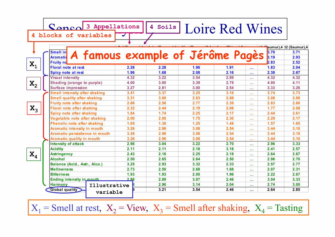
Sensory analysis of 21 Loire Red Wines3 Appellations 4 Soils4 blocks of variables

X

2el (Saumur),1 1cha (Saumur),1 1fon (Bourgueil),1 1vau (Chinon),3 … t1 (Saumur),4 t2 (Saumur),4Smell intensity at rest 3.07 2.96 2.86 2.81 … 3.70 3.71Aromatic quality at rest 3.00 2.82 2.93 2.59 … 3.19 2.93Fruity note at rest 2.71 2.38 2.56 2.42 … 2.83 2.52

A famous example of Jérôme PagèsX1

X2

Floral note at rest 2.28 2.28 1.96 1.91 … 1.83 2.04Spicy note at rest 1.96 1.68 2.08 2.16 … 2.38 2.67Visual intensity 4.32 3.22 3.54 2.89 … 4.32 4.32Shading (orange to purple) 4.00 3.00 3.39 2.79 … 4.00 4.11Surface impression 3.27 2.81 3.00 2.54 … 3.33 3.26S ll i t it ft h ki 3 41 3 37 3 25 3 16 3 74 3 73

X3

Smell intensity after shaking 3.41 3.37 3.25 3.16 … 3.74 3.73Smell quality after shaking 3.31 3.00 2.93 2.88 … 3.08 2.88Fruity note after shaking 2.88 2.56 2.77 2.39 … 2.83 2.60Floral note after shaking 2.32 2.44 2.19 2.08 … 1.77 2.08Spicy note after shaking 1.84 1.74 2.25 2.17 … 2.44 2.61Vegetable note after shaking 2 00 2 00 1 75 2 30 2 29 2 17Vegetable note after shaking 2.00 2.00 1.75 2.30 … 2.29 2.17Phenolic note after shaking 1.65 1.38 1.25 1.48 … 1.57 1.65Aromatic intensity in mouth 3.26 2.96 3.08 2.54 … 3.44 3.10Aromatic persisitence in mouth 3.26 2.96 3.08 2.54 … 3.44 3.10Aromatic quality in mouth 3.26 2.96 3.08 2.54 … 3.44 3.10Intensity of attack 2.96 3.04 3.22 2.70 … 2.96 3.33yAcidity 2.11 2.11 2.18 3.18 … 2.41 2.57Astringency 2.43 2.18 2.25 2.18 … 2.64 2.67Alcohol 2.50 2.65 2.64 2.50 … 2.96 2.70Balance (Acid., Astr., Alco.) 3.25 2.93 3.32 2.33 … 2.57 2.77Mellowness 2.73 2.50 2.68 1.68 … 2.07 2.31

X4

Bitterness 1.93 1.93 2.00 1.96 … 2.22 2.67Ending intensity in mouth 2.86 2.89 3.07 2.46 … 3.04 3.33Harmony 3.14 2.96 3.14 2.04 … 2.74 3.00Global quality 3.39 3.21 3.54 2.46 … 2.64 2.85

Illustrativevariable

X1 = Smell at rest, X2 = View, X3 = Smell after shaking, X4 = Tasting

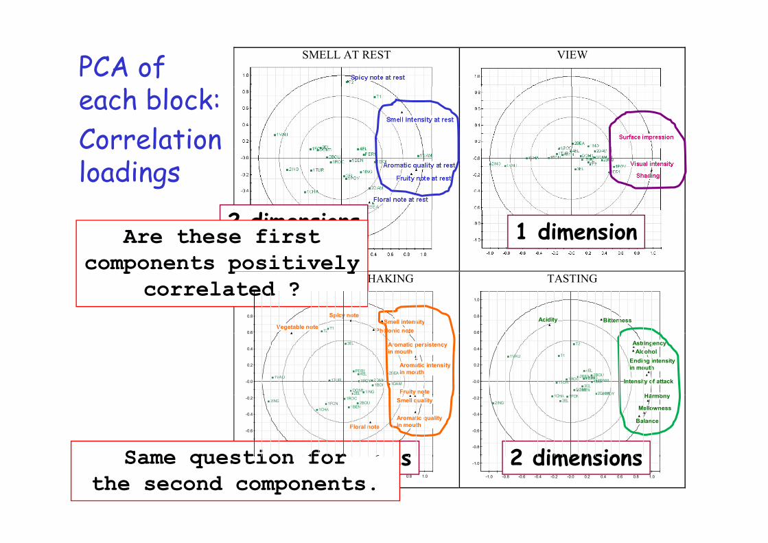
PCA of SMELL AT REST VIEW

each block:CorrelationCorrelationloadings

2 dimensions 1 dimensionAre these firstcomponents positively

SMELL AFTER SHAKING

0 6

0.8

1.0

Smell intensitySpicy note

Vegetable note Phelonic noteT1T20 6

0.8

1.0

Smell intensitySpicy note

Vegetable note Phelonic noteT1T2

TASTING

0 6

0.8

1.0

Acidity Bitterness

0 6

0.8

1.0

Acidity Bitterness

p p ycorrelated ?

-0.0

0.2

0.4

0.6

Fruity note

Aromatic intensityin mouth

Aromatic persistencyin mouth

2EL

1VAU1DAM1BOI

3EL

DOM1

1TUR4EL

PER1

2DAM1POY

1ING

2BEA

-0.0

0.2

0.4

0.6

Fruity note

Aromatic intensityin mouth

Aromatic persistencyin mouth

2EL

1VAU1DAM1BOI

3EL

DOM1

1TUR4EL

PER1

2DAM1POY

1ING

2BEA

-0.0

0.2

0.4

0.6

Intensity of attack

AstringencyAlcohol

Ending intensityin mouth

H1CHA 1FON

1VAU

1DAM2BOU1BOI

3ELDOM1

1TUR

4EL

PER1

2DAM1POY

1ING

1BEN

2BEA1ROC

T1

T2

-0.0

0.2

0.4

0.6

Intensity of attack

AstringencyAlcohol

Ending intensityin mouth

H1CHA 1FON

1VAU

1DAM2BOU1BOI

3ELDOM1

1TUR

4EL

PER1

2DAM1POY

1ING

1BEN

2BEA1ROC

T1

T2

-0.8

-0.6

-0.4

-0.2 Smell quality

Floral noteAromatic qualityin mouth

1CHA1FON 2BOU

1BEN

1ROC2ING

-0.8

-0.6

-0.4

-0.2 Smell quality

Floral noteAromatic qualityin mouth

1CHA1FON 2BOU

1BEN

1ROC2ING

-0.8

-0.6

-0.4

-0.2

Balance

Mellowness

Harmony2EL

1CHA 1FON 1POY

2ING

-0.8

-0.6

-0.4

-0.2

Balance

Mellowness

Harmony2EL

1CHA 1FON 1POY

2ING

2 dimensions 2 dimensionsSame question for-1.0

-1.0 -0.8 -0.6 -0.4 -0.2 -0.0 0.2 0.4 0.6 0.8 1.0

-1.0

-1.0 -0.8 -0.6 -0.4 -0.2 -0.0 0.2 0.4 0.6 0.8 1.0

-1.0

-1.0 -0.8 -0.6 -0.4 -0.2 -0.0 0.2 0.4 0.6 0.8 1.0

-1.0

-1.0 -0.8 -0.6 -0.4 -0.2 -0.0 0.2 0.4 0.6 0.8 1.0

2 dimensions 2 dimensionsSame question forthe second components.

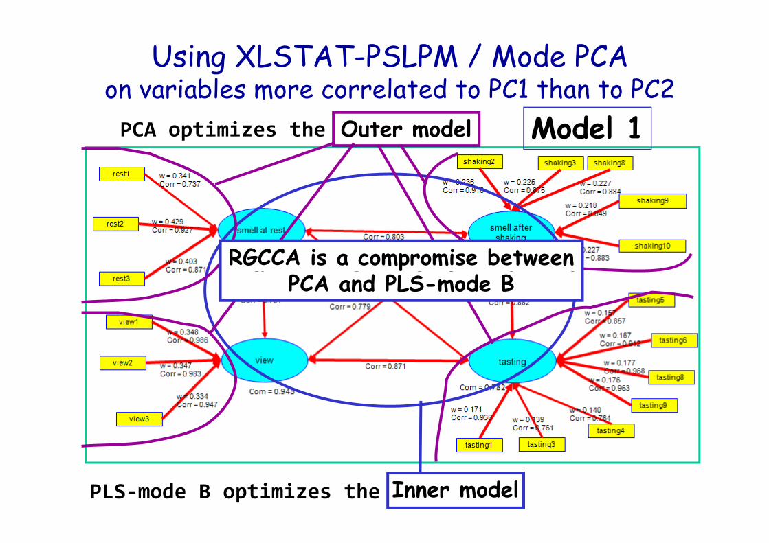
Using XLSTAT-PSLPM / Mode PCAon variables more correlated to PC1 than to PC2 on variables more correlated to PC1 than to PC2

Outer modelPCA optimizes the Model 1

RGCCA is a compromise betweenPCA and PLS-mode B

Inner modelPLS‐mode B optimizes the

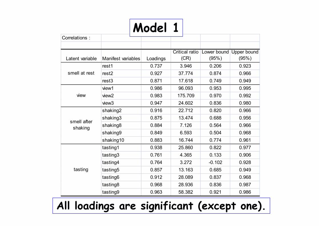
C l tiModel 1

Correlations :

Latent variable Manifest variables LoadingsCritical ratio

(CR)Lower bound

(95%)Upper bound

(95%)rest1 0.737 3.946 0.206 0.923rest2 0.927 37.774 0.874 0.966rest3 0.871 17.618 0.749 0.949view1 0 986 96 093 0 953 0 995

smell at rest

view1 0.986 96.093 0.953 0.995view2 0.983 175.709 0.970 0.992view3 0.947 24.602 0.836 0.980shaking2 0.916 22.712 0.820 0.966

view

gshaking3 0.875 13.474 0.688 0.956shaking8 0.884 7.126 0.564 0.966shaking9 0.849 6.593 0.504 0.968h ki 10 0 883 16 744 0 774 0 961

smell after shaking

shaking10 0.883 16.744 0.774 0.961tasting1 0.938 25.860 0.822 0.977tasting3 0.761 4.365 0.133 0.906tasting4 0.764 3.272 -0.102 0.928gtasting5 0.857 13.163 0.685 0.949tasting6 0.912 28.089 0.837 0.968tasting8 0.968 28.936 0.836 0.987

tasting

tasting9 0.963 58.382 0.921 0.986

All loadings are significant (except one).

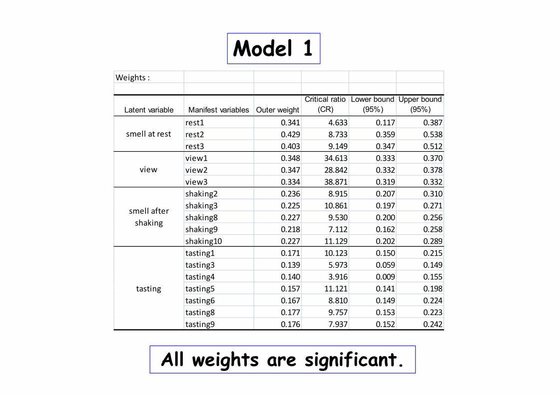
Model 1Weights :

L t t i bl M if t i bl O t i htCritical ratio

(CR)Lower bound

(95%)Upper bound

(95%)Latent variable Manifest variables Outer weight (CR) (95%) (95%)

rest1 0.341 4.633 0.117 0.387rest2 0.429 8.733 0.359 0.538rest3 0.403 9.149 0.347 0.512

smell at rest


view

gshaking3 0.225 10.861 0.197 0.271shaking8 0.227 9.530 0.200 0.256shaking9 0.218 7.112 0.162 0.258shaking10 0 227 11 129 0 202 0 289

smell after shaking

shaking10 0.227 11.129 0.202 0.289tasting1 0.171 10.123 0.150 0.215tasting3 0.139 5.973 0.059 0.149tasting4 0.140 3.916 0.009 0.155tasting5 0 157 11 121 0 141 0 198tasting tasting5 0.157 11.121 0.141 0.198tasting6 0.167 8.810 0.149 0.224tasting8 0.177 9.757 0.153 0.223tasting9 0.176 7.937 0.152 0.242

tasting

All weights are significant.

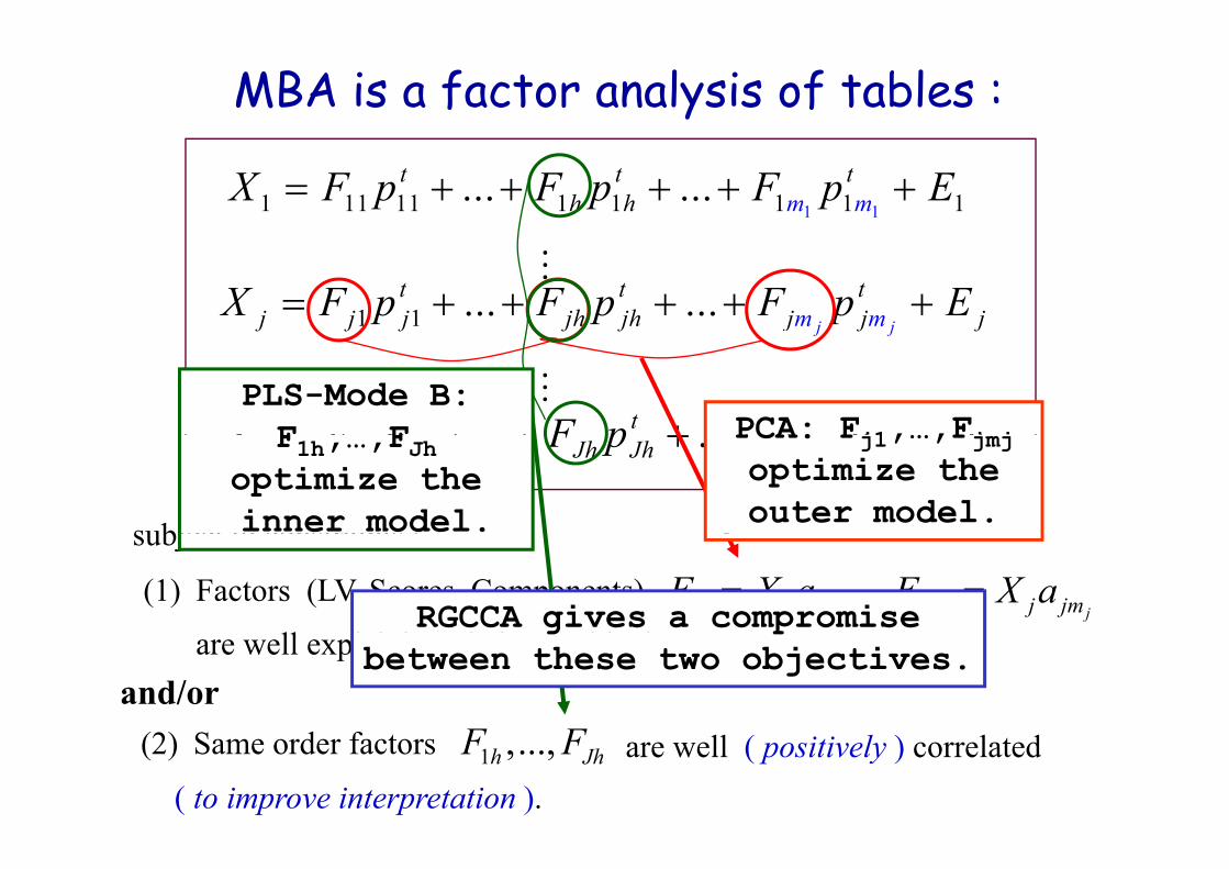
MBA is a factor analysis of tables :

1 11 11 11 1 1 1 1 1... ... m mt t t

h hX F p F p F p E= + + + + +

1 1 ... ...j j

t t tj j j jh j mj jmh jX F p F p F p E= + + + + +

j j

t t tX F p F p F p E= + + + + +PCA: Fj1, ,Fj j

PLS-Mode B: F F

subject to constraints :

1 1 ... ...J JJ J J Jh J mJ Jmh JX F p F p F p E= + + + + +PCA: Fj1,…,Fjmj

optimize theouter model.

F1h,…,FJhoptimize theinner model.

(1) Factors (LV, Scores, Components)

subject to constraints :

1 1,..., j jj j j jm j jmF X a F X a= =RGCCA gives a compromise

are well explaining their own block .

F Fand/or

g pbetween these two objectives.

(2) Same order factors 1 ,...,h JhF F are well ( positively ) correlated( to improve interpretation ).

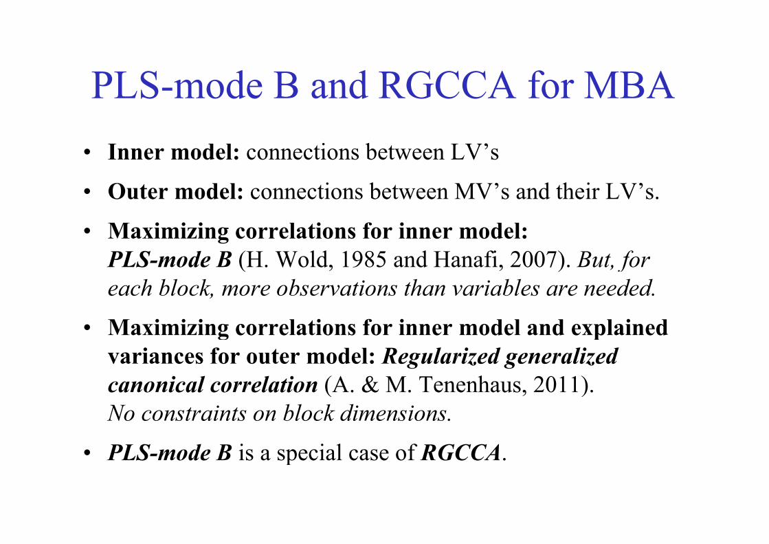
PLS mode B and RGCCA for MBAPLS-mode B and RGCCA for MBAInner model: connections bet een LV’s• Inner model: connections between LV’s

• Outer model: connections between MV’s and their LV’s.

• Maximizing correlations for inner model: PLS-mode B (H. Wold, 1985 and Hanafi, 2007). But, for feach block, more observations than variables are needed.

• Maximizing correlations for inner model and explainedMaximizing correlations for inner model and explained variances for outer model: Regularized generalized canonical correlation (A. & M. Tenenhaus, 2011). ( , )No constraints on block dimensions.

• PLS-mode B is a special case of RGCCAPLS mode B is a special case of RGCCA.

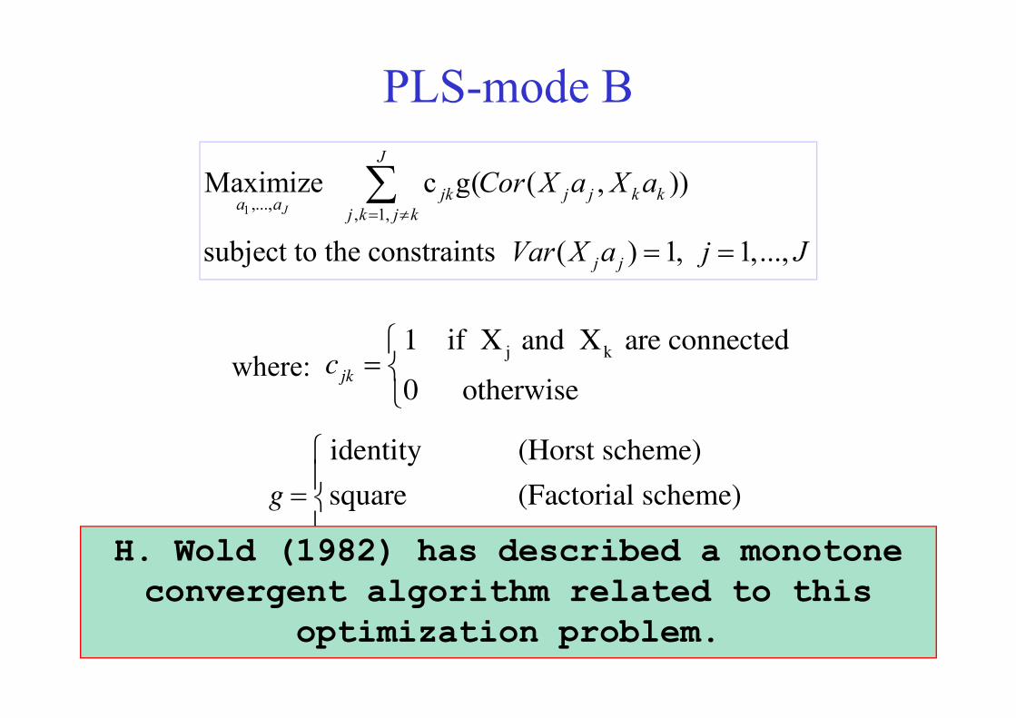
PLS-mode B

Maximize c g( ( , ))J

jk j j k kCor X a X a∑1 ,..., , 1,

g( ( , ))

subject to the constraints ( ) 1, 1,...,J

jk j j k ka a j k j k

j jVar X a j J= ≠

= =

∑

h⎧⎨

j k1 if X and X are connectedwhere: = ⎨

⎩

j

0 otherwise jkc

⎧id i (H h )⎧⎪= ⎨⎪

identity (Horst scheme)

square (Factorial scheme)g⎪⎩abolute value (Centroid scheme)H. Wold (1982) has described a monotone

convergent algorithm related to this 9

g goptimization problem.

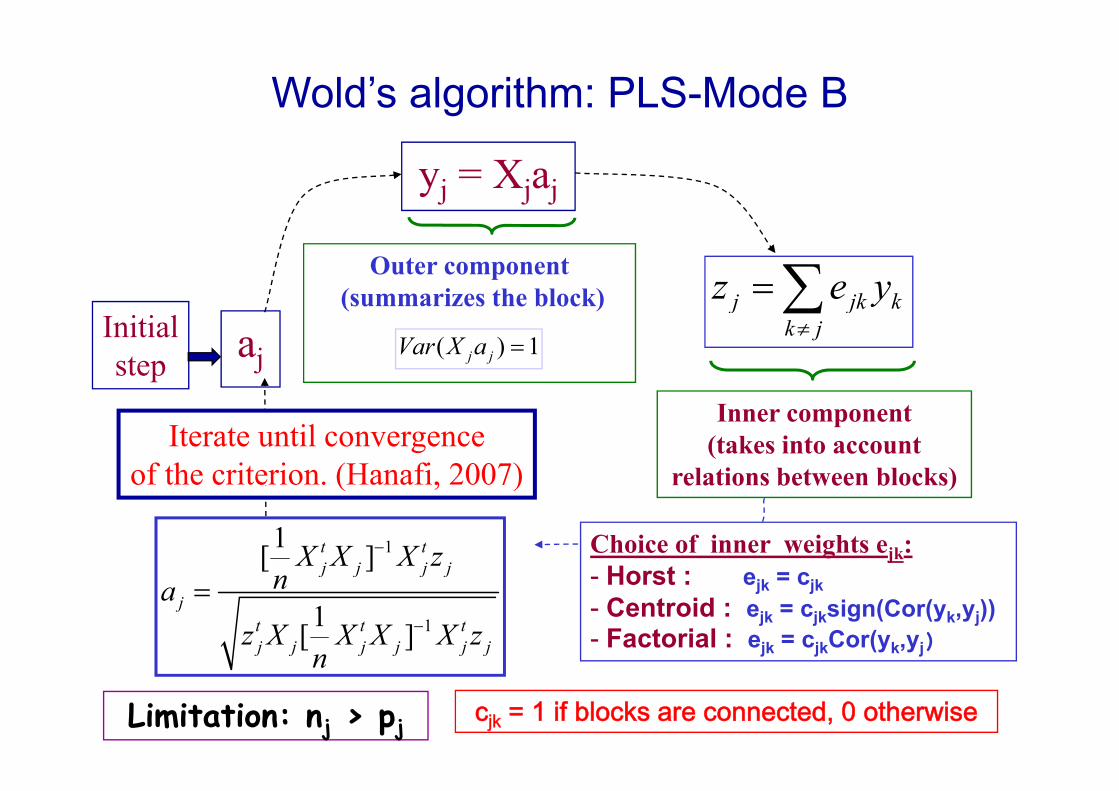
Wold’s algorithm: PLS-Mode B

yj = Xjaj

Outer component(summarizes the block) =∑j jk kz e y

ajInitialstep

(summarizes the block)

( ) 1=j jVar X a≠∑j jk kk j

y

Inner component(takes into account

relations between blocks)Iterate until convergence

of the criterion. (Hanafi, 2007)

11[ ]−t tj j j jX X X z Choice of inner weights ejk:

Horst : e = c

e at o s betwee b oc s)( , )

11[ ]−=

j j j j

jt t tj j j j j j

naz X X X X z

n

- Horst : ejk = cjk- Centroid : ejk = cjksign(Cor(yk,yj)) - Factorial : ejk = cjkCor(yk,yj)n

cjk = 1 if blocks are connected, 0 otherwiseLimitation: nj > pj

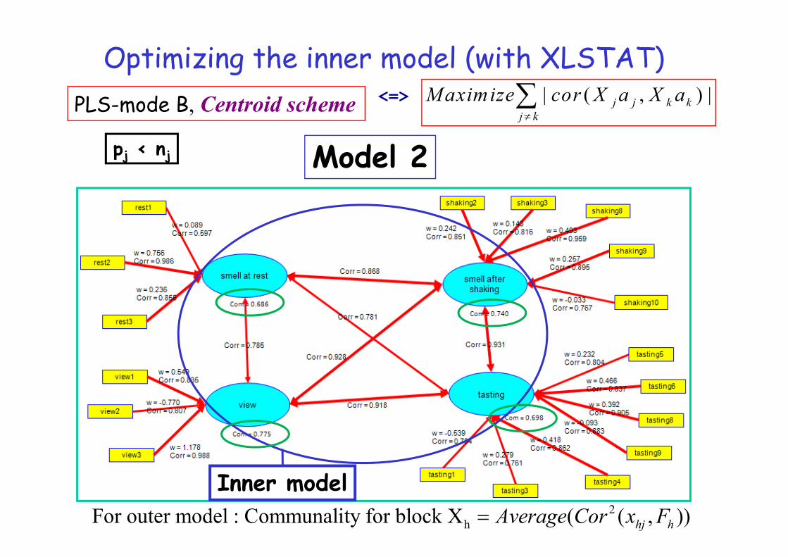
| ( ) |M i i X X∑Optimizing the inner model (with XLSTAT)

PLS-mode B, Centroid scheme | ( , ) |j j k kj k

M aximize cor X a X a≠∑<=>

pj < nj Model 2pj < nj Model 2

Inner model2

hFor outer model : Communality for block X ( ( , ))hj hAverage Cor x F=

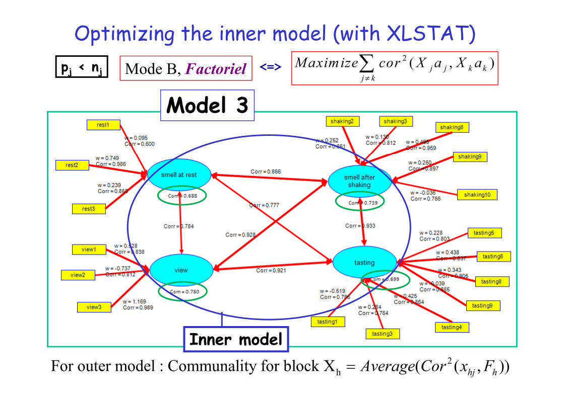
Optimizing the inner model (with XLSTAT)M d B F i l

2 ( )M aximize cor X a X a∑< > Mode B, Factoriel ( , )j j k kj k

M aximize cor X a X a≠∑<=>pj < nj

Model 3Model 3

I d l2

hFor outer model : Communality for block X ( ( , ))hj hAverage Cor x F=

Inner model

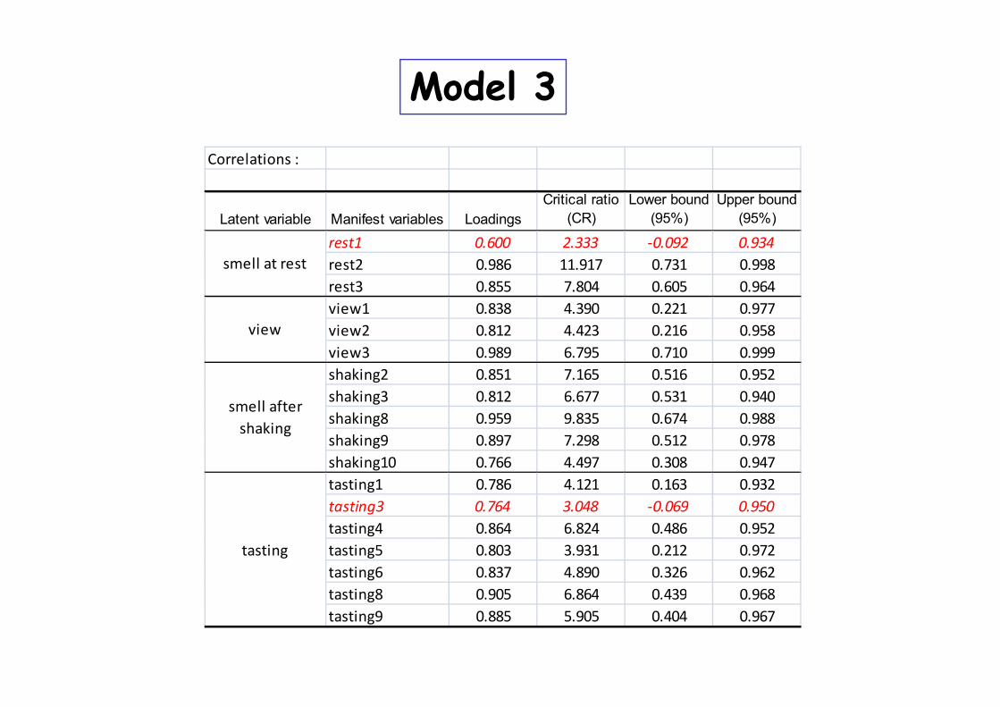
Model 3Correlations :


(CR)Lower bound

(95%)Upper bound

(95%)

rest1 0.600 2.333 ‐0.092 0.934rest2 0.986 11.917 0.731 0.998smell at restrest3 0.855 7.804 0.605 0.964view1 0.838 4.390 0.221 0.977view2 0.812 4.423 0.216 0.958view3 0 989 6 795 0 710 0 999

viewview3 0.989 6.795 0.710 0.999shaking2 0.851 7.165 0.516 0.952shaking3 0.812 6.677 0.531 0.940shaking8 0.959 9.835 0.674 0.988

smell after shaking

shaking9 0.897 7.298 0.512 0.978shaking10 0.766 4.497 0.308 0.947tasting1 0.786 4.121 0.163 0.932tasting3 0.764 3.048 ‐0.069 0.950

g

gtasting4 0.864 6.824 0.486 0.952tasting5 0.803 3.931 0.212 0.972tasting6 0.837 4.890 0.326 0.962tasting8 0 905 6 864 0 439 0 968

tasting

tasting8 0.905 6.864 0.439 0.968tasting9 0.885 5.905 0.404 0.967

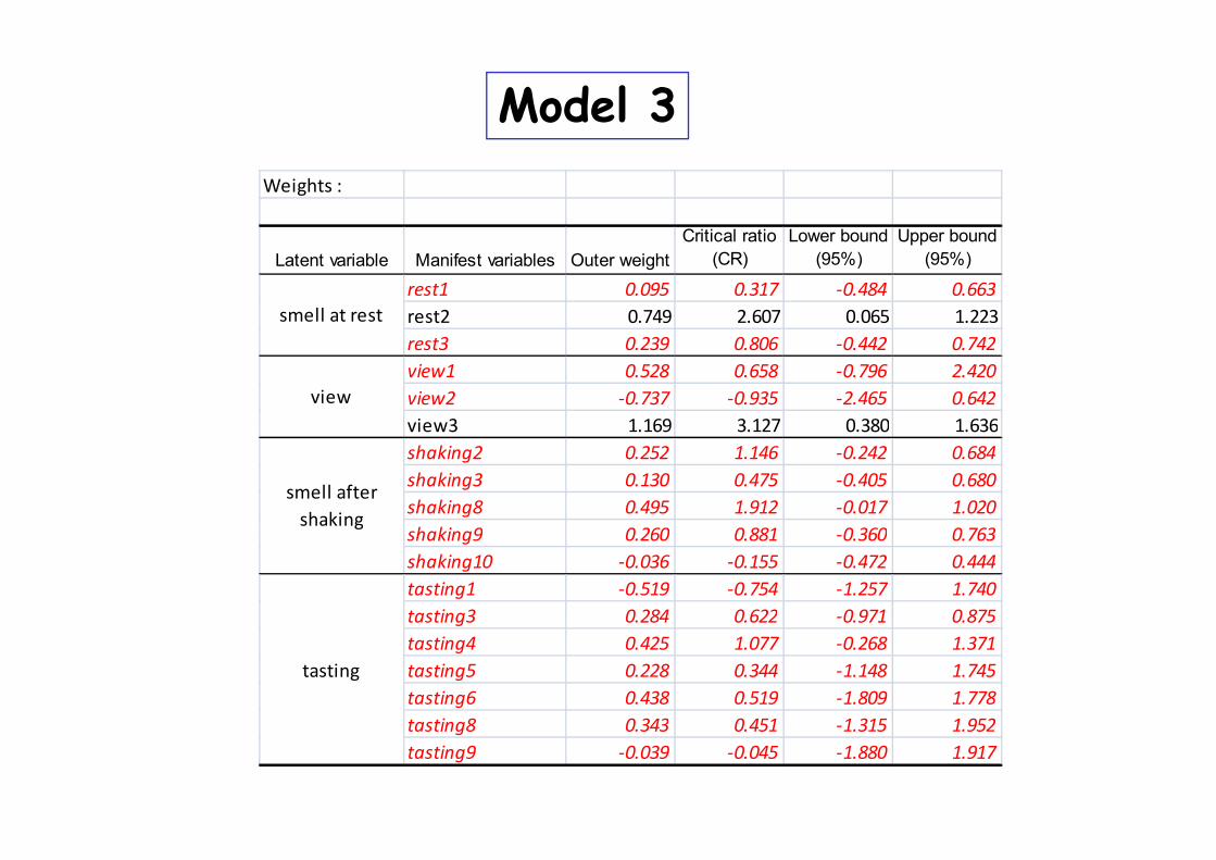
Model 3Weights :

Critical ratio Lower bound Upper boundLatent variable Manifest variables Outer weight

Critical ratio (CR)

Lower bound (95%)

Upper bound (95%)

rest1 0.095 0.317 ‐0.484 0.663rest2 0.749 2.607 0.065 1.223smell at restrest3 0.239 0.806 ‐0.442 0.742view1 0.528 0.658 ‐0.796 2.420view2 ‐0.737 ‐0.935 ‐2.465 0.642view3 1.169 3.127 0.380 1.636

viewview3 1.169 3.127 0.380 1.636shaking2 0.252 1.146 ‐0.242 0.684shaking3 0.130 0.475 ‐0.405 0.680shaking8 0.495 1.912 ‐0.017 1.020h ki 9 0 260 0 88 0 360 0 63

smell after shaking

shaking9 0.260 0.881 ‐0.360 0.763shaking10 ‐0.036 ‐0.155 ‐0.472 0.444tasting1 ‐0.519 ‐0.754 ‐1.257 1.740tasting3 0.284 0.622 ‐0.971 0.875

g

gtasting4 0.425 1.077 ‐0.268 1.371tasting5 0.228 0.344 ‐1.148 1.745tasting6 0.438 0.519 ‐1.809 1.778tasting8 0 343 0 451 1 315 1 952

tasting

tasting8 0.343 0.451 ‐1.315 1.952tasting9 ‐0.039 ‐0.045 ‐1.880 1.917

Conclusion• Many weights are not significant !!!y g g

• If you want the butter(good correlations for the inner and outer models)outer models)and the money of the butter (significant weights) ,you must switch to Regularized you must switch to Regularized Generalized Canonical Correlation

l ( G )Analysis (RGCCA).

Regularized generalized CCARegularized generalized CCA

Maximize c g( ( ))J

Cov X a X a∑1 ,..., , 1,

2

Maximize c g( ( , ))

subject to the constraints (1 ) ( ) 1 1

Jjk j j k ka a j k j k

Cov X a X a

a Var X a j Jτ τ

= ≠

+

∑

subject to the constraints (1 ) ( ) 1, 1,...,j j j j ja Var X a j Jτ τ+ − = =

⎧1 if X d X t dA monotone convergent algorithml d hi i i i bl

where:⎧

= ⎨⎩

j k1 if X and X are connected

0 otherwise jkc

related to this optimization problemis proposed.

⎧⎪= ⎨

identity (Horst scheme)

square (Factorial scheme)g = ⎨⎪⎩

square (Factorial scheme)

abolute value (Centroid scheme)

g

and: Shrinkage constant between 0 and 1jτ = 16

The PLS algorithm for RGCCAyj = Xjaj


ajInitialstep

( )2

(1 ) ( ) 1τ τ+ − =j j j j ja Var X a≠∑j jk kk j

Iterate until convergenceof the criterion.

Inner component(takes into account relations

between blocks)

11[( (1 ) ]τ τ −+ − t tj j j j j jI X X X z

nChoice of inner weights ejk:- Horst : ejk = cjk

)

11[( (1 ) ]τ τ −

=+ −

jt t tj j j j j j j j

naz X I X X X z

n

j j- Centroid : ejk = cjksign(Cor(yk,yj))- Factorial : ejk = cjkCov(yk,yj)

17cjk = 1 if blocks are connected, 0 otherwise.nj can be <= pj,for τj > 0.

All τj = 0, RGCCA = PLS-Mode Byj = Xjaj


ajInitialstep

( )

( ) 1j jVar X a =≠∑j jk kk j



between blocks)

11[ ]t tj j j jX X X z−

Choice of inner weights ejk:- Horst : ejk = cjk

)

11[ ]

j j j j

jt t tj j j j j j

naz X X X X z

n−

=j j

- Centroid : ejk = cjksign(Cor(yk,yj))- Factorial : ejk = cjkCor(yk,yj)

18

ncjk = 1 if blocks are connected, 0 otherwise.

All τj = 1, RGCCA - Mode Ayj = Xjaj


ajInitialstep

( )2

1ja =≠∑j jk kk j



between blocks)

tX zChoice of inner weights ejk:- Horst : ejk = cjk

)

j jj t

j j

X za

X z=

j j- Centroid : ejk = cjksign(Cor(yk,yj))- Factorial : ejk = cjkCov(yk,yj)

19cjk = 1 if blocks are connected, 0 otherwise.nj can be <= pj.

Model 4 : RGCCA, factorial scheme, mode A 2

1,

cov ( , )j

j j k kj ka j

M aximize X a X a≠= ∀

∑,j j

Latent variables have been afterwards standardized.

Model 4Correlations :


(CR)Lower bound

(95%)Upper bound

(95%)Latent variable Manifest variables Loadings (CR) (95%) (95%)

rest1 0.708 3.301 0.113 0.924rest2 0.938 31.414 0.880 0.970rest3 0.880 20.537 0.776 0.954

smell at rest

view1 0.983 21.303 0.898 0.995view2 0.980 28.635 0.937 0.993view3 0.954 34.009 0.883 0.982shaking2 0 904 22 231 0 810 0 965

view

shaking2 0.904 22.231 0.810 0.965shaking3 0.862 11.238 0.669 0.957shaking8 0.900 14.572 0.753 0.972shaking9 0.869 9.636 0.662 0.972

smell after shaking

shaking10 0.870 14.582 0.715 0.964tasting1 0.936 14.373 0.693 0.978tasting3 0.773 5.563 0.423 0.911tasting4 0.776 4.980 0.361 0.930gtasting5 0.848 9.118 0.582 0.958tasting6 0.904 17.424 0.767 0.972tasting8 0.970 30.511 0.879 0.989t ti 9 0 959 31 991 0 864 0 986

tasting

All loadings are significant.tasting9 0.959 31.991 0.864 0.986

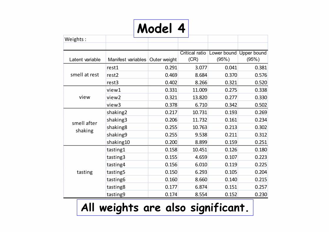
Model 4Weights :

Latent variable Manifest variables Outer weightCritical ratio

(CR)Lower bound

(95%)Upper bound

(95%)

rest1 0.291 3.077 0.041 0.381rest2 0.469 8.684 0.370 0.576rest3 0.402 8.266 0.321 0.520view1 0 331 11 009 0 275 0 338

smell at rest


view

shaking3 0.206 11.732 0.161 0.234shaking8 0.255 10.763 0.213 0.302shaking9 0.255 9.538 0.211 0.312shaking10 0 200 8 899 0 159 0 251

smell after shaking

shaking10 0.200 8.899 0.159 0.251tasting1 0.158 10.451 0.126 0.180tasting3 0.155 4.659 0.107 0.223tasting4 0.156 6.010 0.119 0.225tasting5 0.150 6.293 0.105 0.204tasting6 0.160 8.660 0.140 0.215tasting8 0.177 6.874 0.151 0.257tasting9 0 174 8 554 0 152 0 230

tasting

tasting9 0.174 8.554 0.152 0.230

All weights are also significant.

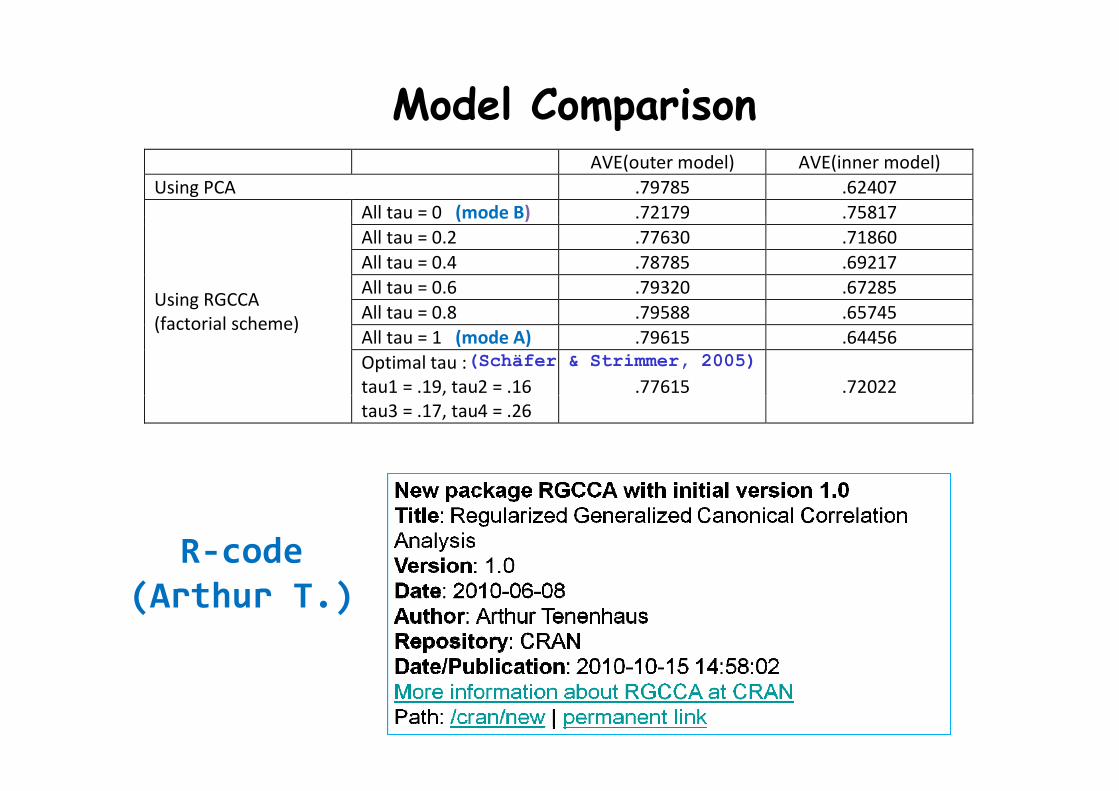
Model Comparisonp AVE(outer model) AVE(inner model)Using PCA .79785 .62407

All tau = 0 (mode B) 72179 75817

Using RGCCA

All tau 0 (mode B) .72179 .75817All tau = 0.2 .77630 .71860All tau = 0.4 .78785 .69217All tau = 0.6 .79320 .67285ll

(Schäfer & Strimmer, 2005)

Us g G(factorial scheme) All tau = 0.8 .79588 .65745

All tau = 1 (mode A) .79615 .64456Optimal tau :tau1 = .19, tau2 = .16 .77615 .72022,tau3 = .17, tau4 = .26

R‐code(Arthur T.)

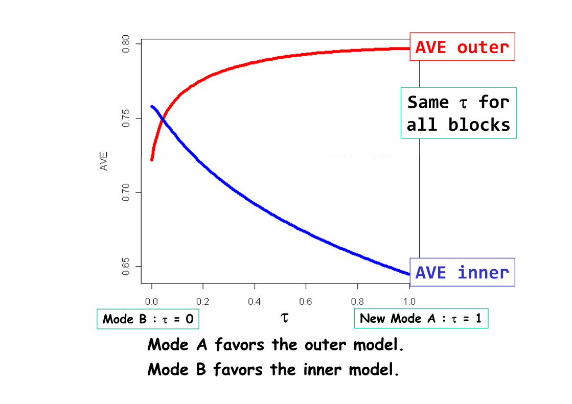
AVE outer

Same τ forall blocks

AVE inner

M d A f th t d l τMode B : τ = 0 New Mode A : τ = 1

Mode A favors the outer model. Mode B favors the inner model.

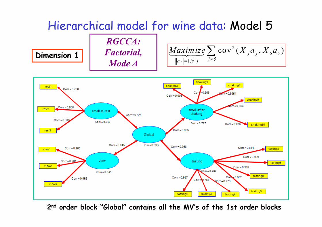
Hierarchical model for wine data: Model 5

Dimension 1

RGCCA: Factorial, M d A

25 5

51,

cov ( , )j

j jja j


∑Mode A 1, ja j∀

2nd order block “Global” contains all the MV’s of the 1st order blocks

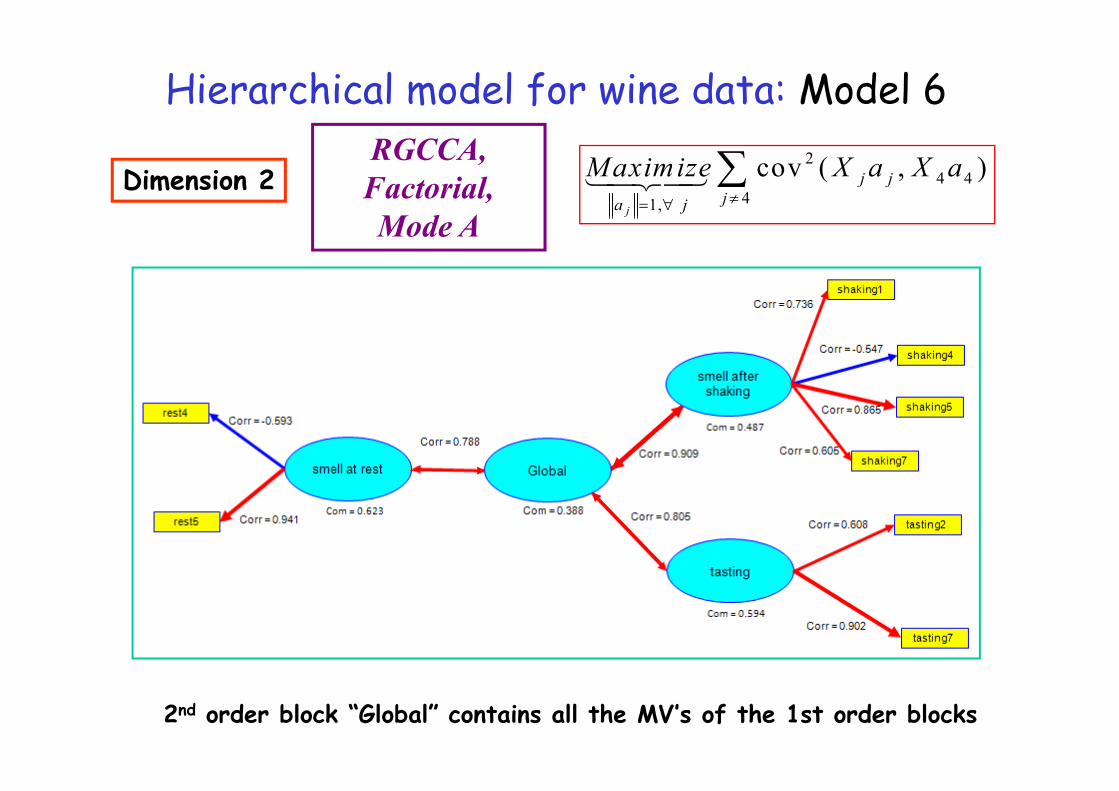
Hierarchical model for wine data: Model 6

Dimension 2RGCCA, Factorial, M d A

24 4

41,

cov ( , )j

j jja j


∑Mode A

j

2nd order block “Global” contains all the MV’s of the 1st order blocks

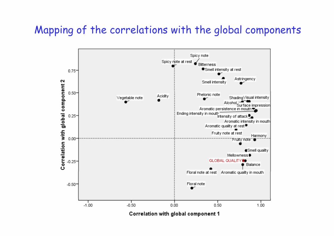
Mapping of the correlations with the global components

Wine visualization in the global component spaceWi k d b ll iWines marked by Appellation

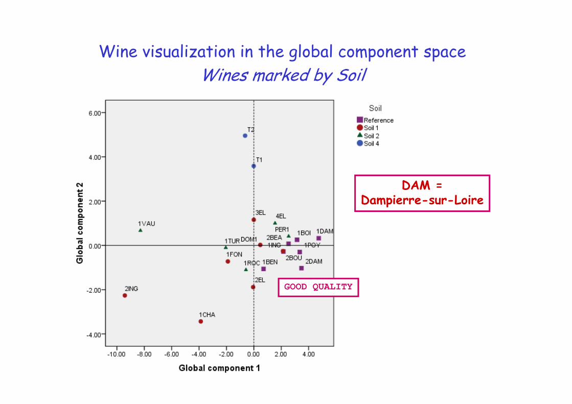
Wine visualization in the global component spaceWines marked by Soil

DAM =Dampierre-sur-LoireDampierre sur Loire

GOOD QUALITY

Cuvée Lisagathe 1995

A soft, warm, blackberry nose. A good core of fruit on the palate with quite well worked tannin and acidity on the finish; Good l th d l t f t ti llength and a lot of potential.

DECANTER (mai 1997)(DECANTER AWARD ***** : Outstanding quality, a virtually perfect example)

ReferencesReferences

Fi l l iFinal conclusion

All the proofs of a pudding are in the eating butAll the proofs of a pudding are in the eating, butit will taste even better if you know the cooking.

32

pls path modeling and rgcca for multi-block data … · pls path modeling and rgcca for multi-block...

Documents