pm2.5 continuous monitoring assessing the data · pm 2.5 continuous monitoring assessing the data...

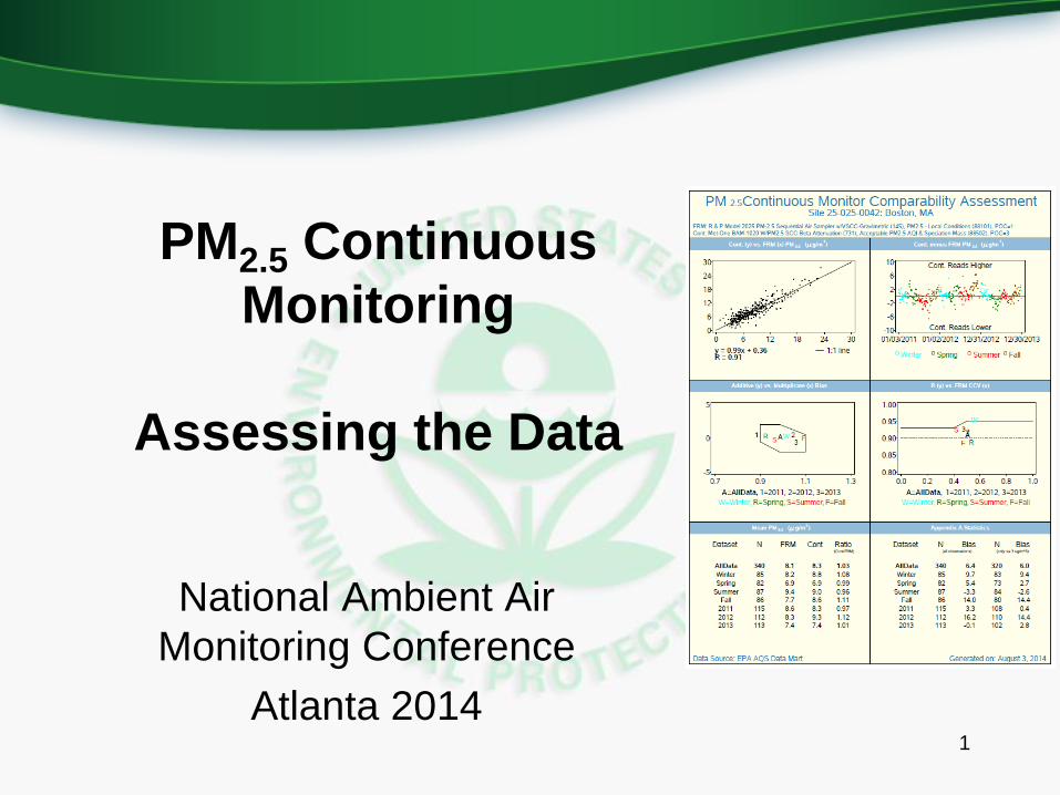
PM2.5 Continuous

Monitoring

Assessing the Data

National Ambient Air

Monitoring Conference

Atlanta 20141

Approach for this section:

Take a step by step approach to assess

whether your getting good PM2.5 continuous

FEM data

1. Ensure your getting good FRM data

2. Review and assess your data.

3. Use automated assessment tools

4. Know what to expect for acceptable performance

from a PM2.5 Continuous Monitor, and

5. What to expect in your data by Method

6. Look at the data in more detail2

Ensure your getting good FRM data

You won’t know if your getting PM2.5 Continuous FEM

data unless you know your program is getting good

FRM data

Lab – Field Blank data

Collocated Precision

Performance Audits (with collocated FRMs)

3

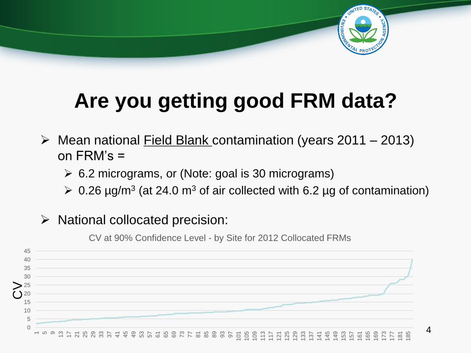
Are you getting good FRM data?

Mean national Field Blank contamination (years 2011 – 2013)

on FRM’s =

6.2 micrograms, or (Note: goal is 30 micrograms)

0.26 µg/m3 (at 24.0 m3 of air collected with 6.2 µg of contamination)

National collocated precision:

40

5

10

15

20

25

30

35

40

45

1 5 9

13

17

21

25

29

33

37

41

45

49

53

57

61

65

69

73

77

81

85

89

93

97

101

105

109

113

117

121

125

129

133

137

141

145

149

153

157

161

165

169

173

177

181

185

CV at 90% Confidence Level - by Site for 2012 Collocated FRMs

CV

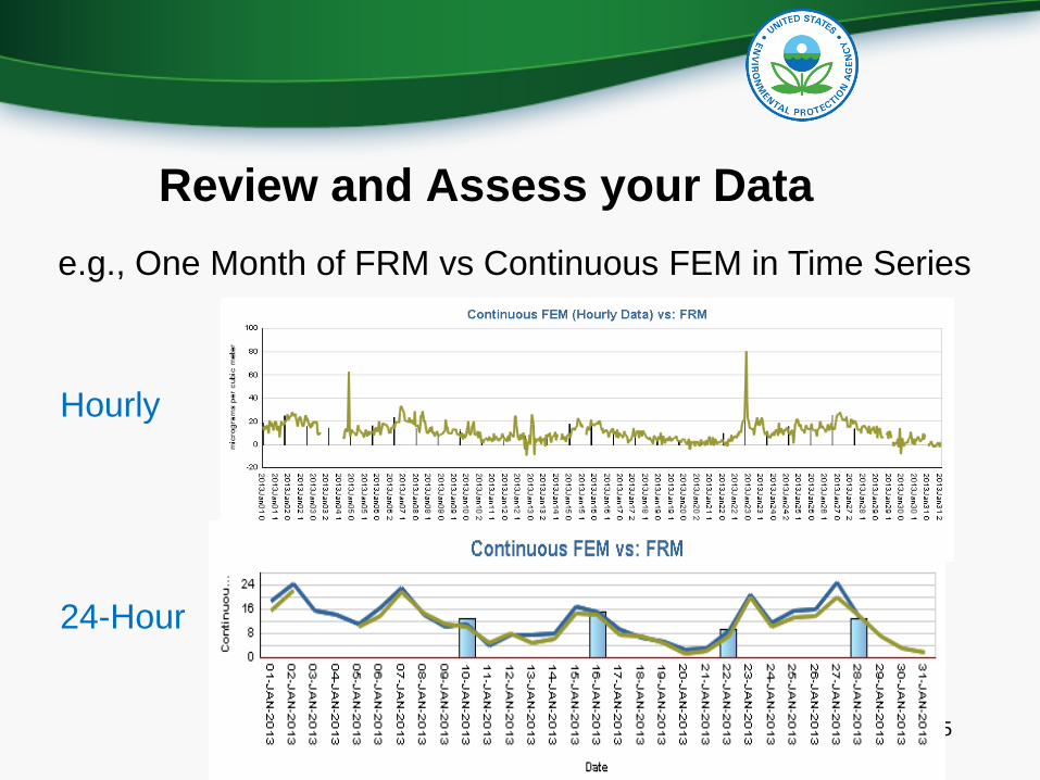
Review and Assess your Data

5

e.g., One Month of FRM vs Continuous FEM in Time Series

24-Hour

Hourly

Utilize Comparability Assessment Tools

6

Candidate FEM Excel File One-Page

Automated Assessment

http://www.epa.gov/ttn/amtic/contmont.html

• Four variations of same file available

• Blank file for up to 70, 122, or 366

collocated pairs

• Example file

• You have to supply the data

= or

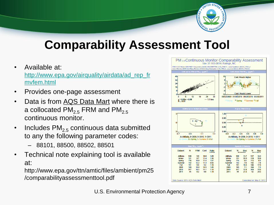
Comparability Assessment Tool

• Available at: http://www.epa.gov/airquality/airdata/ad_rep_fr

mvfem.html

• Provides one-page assessment

• Data is from AQS Data Mart where there is

a collocated PM2.5 FRM and PM2.5

continuous monitor.

• Includes PM2.5 continuous data submitted

to any the following parameter codes:

– 88101, 88500, 88502, 88501

• Technical note explaining tool is available

at: http://www.epa.gov/ttn/amtic/files/ambient/pm25

/comparabilityassessmenttool.pdf

U.S. Environmental Protection Agency 7

http://www.epa.gov/airquality/airdata/ad_rep_frmvfem.html

PM2.5 Continuous Monitor Comparability Assessment Tool

8

Linear

Regression

Part 53

Test

Specifications

Data

Summary

Difference

Trend

Correlation

Criteria

Appendix A

9

Title, Site, Methods, and Difference Trend

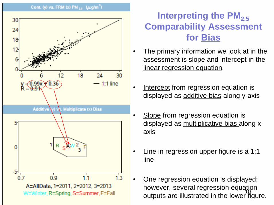
• The primary information we look at in the

assessment is slope and intercept in the

linear regression equation.

• Intercept from regression equation is

displayed as additive bias along y-axis

• Slope from regression equation is

displayed as multiplicative bias along x-

axis

• Line in regression upper figure is a 1:1

line

• One regression equation is displayed;

however, several regression equation

outputs are illustrated in the lower figure.10

Interpreting the PM2.5

Comparability Assessment

for Bias

11

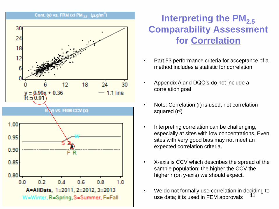
• Part 53 performance criteria for acceptance of a

method includes a statistic for correlation

• Appendix A and DQO’s do not include a

correlation goal

• Note: Correlation (r) is used, not correlation

squared (r2)

• Interpreting correlation can be challenging,

especially at sites with low concentrations. Even

sites with very good bias may not meet an

expected correlation criteria.

• X-axis is CCV which describes the spread of the

sample population; the higher the CCV the

higher r (on y-axis) we should expect.

• We do not formally use correlation in deciding to

use data; it is used in FEM approvals 11

Interpreting the PM2.5

Comparability Assessment

for Correlation

12

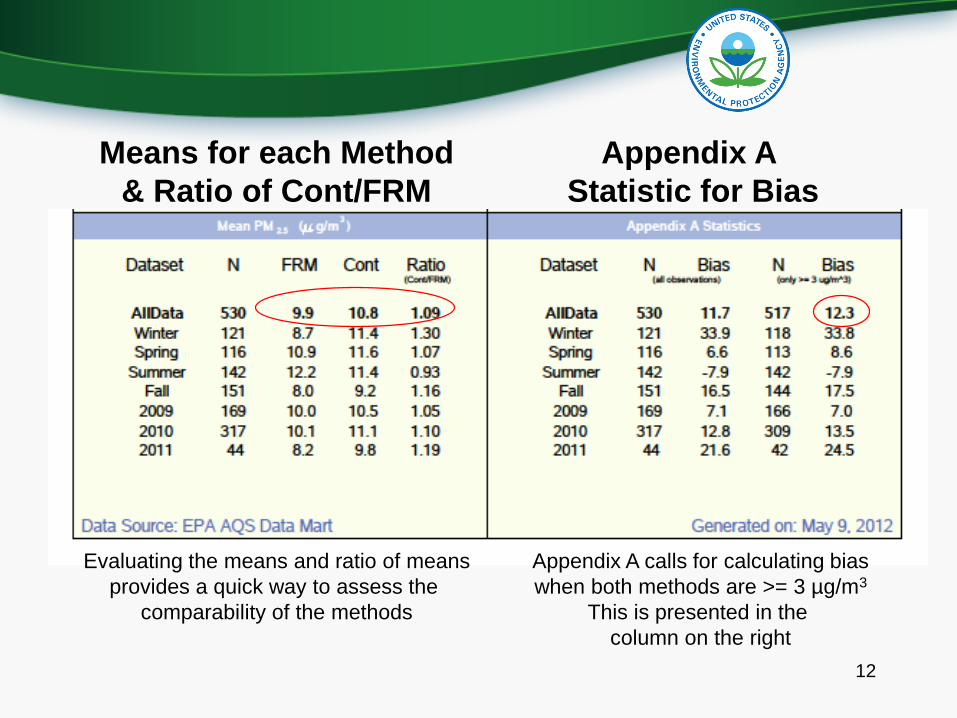
Evaluating the means and ratio of means

provides a quick way to assess the

comparability of the methods

Appendix A calls for calculating bias

when both methods are >= 3 µg/m3

This is presented in the

column on the right

Means for each Method

& Ratio of Cont/FRM

Appendix A

Statistic for Bias

Comparability Assessment Tool Summary

• Tool provides quick and valuable assessment

• The assessment assumes the FRM represents the true value, even

though the FRM will have its own uncertainty

• Assessments should be used as a guide and not a bright line

From Section 2.3.1.1 of Appendix A to Part 58:

Measurement Uncertainty for Automated and Manual PM2.5 Methods.

The goal for acceptable measurement uncertainty is defined as 10 percent

coefficient of variation (CV) for total precision and plus or minus 10

percent for total bias

Appendix A calculation of Bias is based on samples collected in Performance

Evaluation Program (PEP) program (PEP data are not included in one page

assessment)

U.S. Environmental Protection Agency 13

Data Challenges

1. Interpreting performance data as air quality levels keep

improving.

2. Knowing what to expect in data from a method?

3. Negative Numbers

4. Additional Data Assessment Details

14

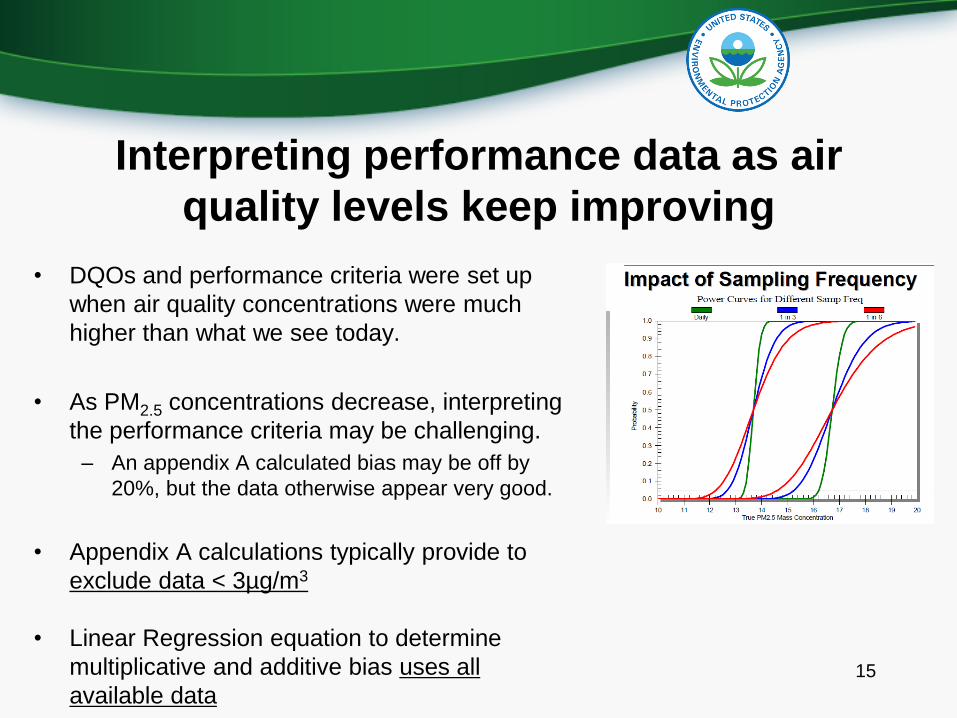
Interpreting performance data as air

quality levels keep improving

• DQOs and performance criteria were set up

when air quality concentrations were much

higher than what we see today.

• As PM2.5 concentrations decrease, interpreting

the performance criteria may be challenging.

– An appendix A calculated bias may be off by

20%, but the data otherwise appear very good.

• Appendix A calculations typically provide to

exclude data < 3µg/m3

• Linear Regression equation to determine

multiplicative and additive bias uses all

available data15

What to Expect for Acceptable Performance

from a PM2.5 Continuous Monitor?• Bias:

– Drives decision errors

– Ideally, total bias is within within +/- 10%

– A goal, not a requirement; however,

– Certain monitors may be excluded from NAAQS if they do not

meet total bias and are approved for exclusion.

• Precision:

– Does not drive decision errors due to large data set with an

effective daily sample schedule

– Class III Continuous method precision criteria is within 15%

• Correlation

– Used in Class III Method approvals based on sample

population

– From 2002 AQI DQO Document we established a goal for an

R of 0.9 (R2 = 0.81)

– However, as previously stated correlation can be hard to

interpret at low air quality concentrations16

What to expect in your data by Method –

Looking at available data

• Large collocated data set available to

evaluate Met One BAM 1020

• Smaller collocated data sets available for

FDMS 8500C and 5030 SHARP

• Very little collocated data sets available for

the rest of the methods.

17

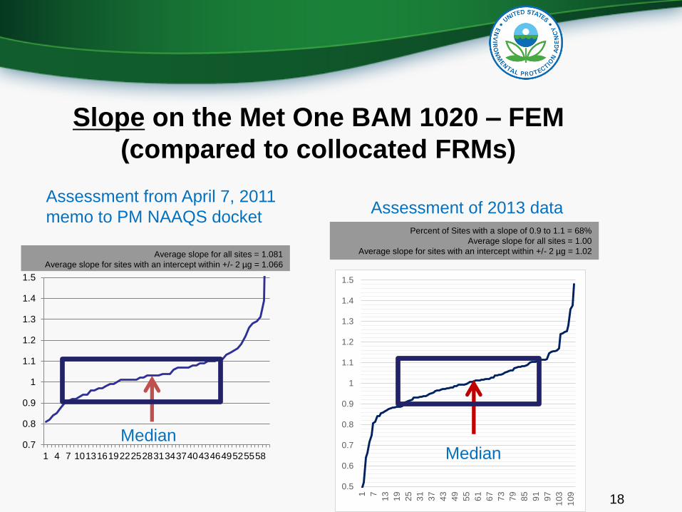
Slope on the Met One BAM 1020 – FEM

(compared to collocated FRMs)

180.5

0.6

0.7

0.8

0.9

1

1.1

1.2

1.3

1.4

1.5

1 7

13

19

25

31

37

43

49

55

61

67

73

79

85

91

97

103

109

Assessment of 2013 data

0.7

0.8

0.9

1

1.1

1.2

1.3

1.4

1.5

1 4 7 1013161922252831343740434649525558

Average slope for all sites = 1.081

Average slope for sites with an intercept within +/- 2 µg = 1.066

Assessment from April 7, 2011

memo to PM NAAQS docketPercent of Sites with a slope of 0.9 to 1.1 = 68%



MedianMedian

-3

-2

-1

0

1

2

3

4

5

6

1 6

11

16

21

26

31

36

41

46

51

56

61

66

71

76

81

86

91

96

101

106

111

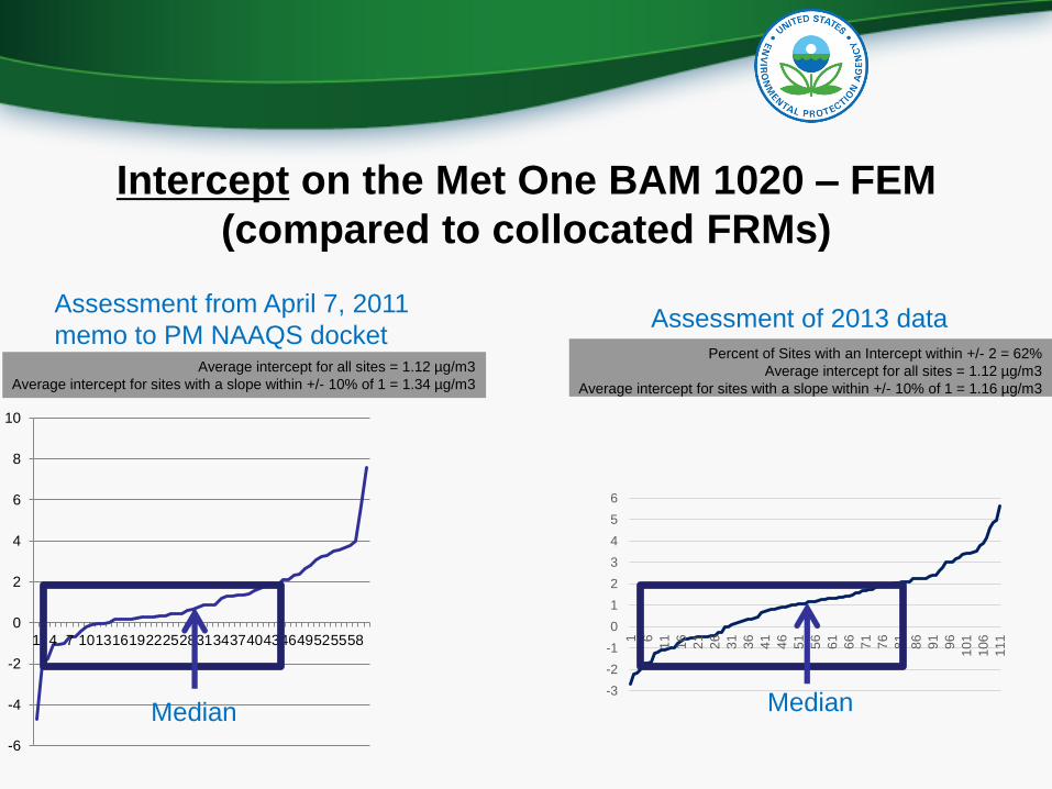
Intercept on the Met One BAM 1020 – FEM


-6

-4

-2

0

2

4

6

8

10

1 4 7 1013161922252831343740434649525558

Average intercept for all sites = 1.12 µg/m3

Average intercept for sites with a slope within +/- 10% of 1 = 1.34 µg/m3

Percent of Sites with an Intercept within +/- 2 = 62%




memo to PM NAAQS docketAssessment of 2013 data

Median Median

Median

0.4

0.5

0.6

0.7

0.8

0.9

1

1.1

1.2

1.3

1.4

1 2 3 4 5 6 7 8 9 10 11 12 13 14 15 16 17

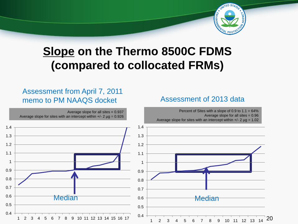
Slope on the Thermo 8500C FDMS


20

Assessment of 2013 dataAssessment from April 7, 2011

memo to PM NAAQS docket

Percent of Sites with a slope of 0.9 to 1.1 = 64%



Median



0.4

0.5

0.6

0.7

0.8

0.9

1

1.1

1.2

1.3

1.4

1 2 3 4 5 6 7 8 9 10 11 12 13 14

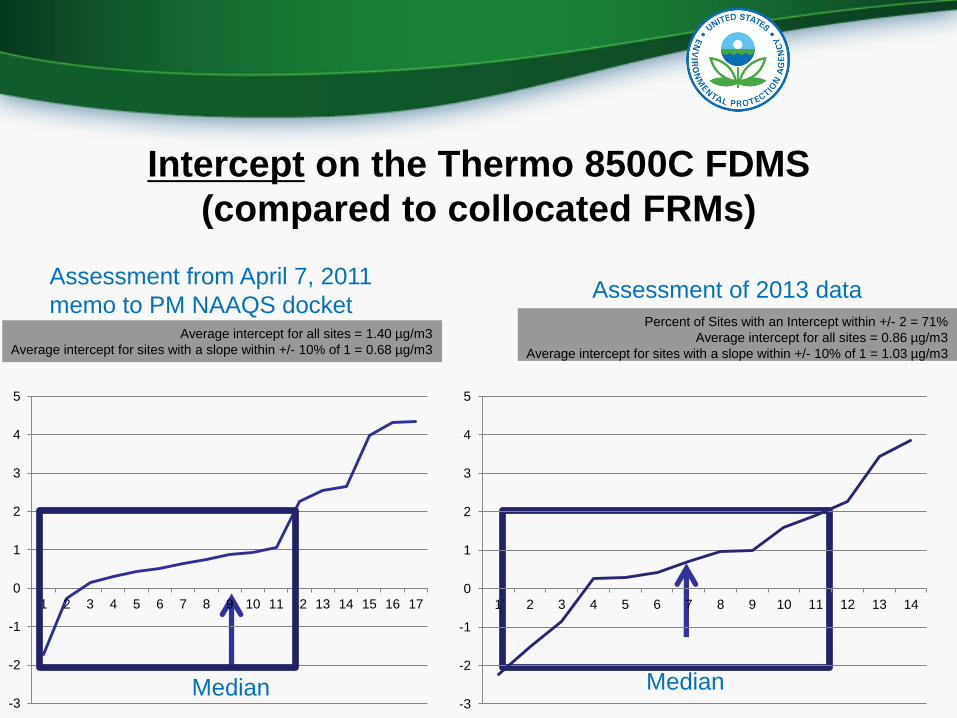
Intercept on the Thermo 8500C FDMS




Percent of Sites with an Intercept within +/- 2 = 71%




memo to PM NAAQS docketAssessment of 2013 data

-3

-2

-1

0

1

2

3

4

5

1 2 3 4 5 6 7 8 9 10 11 12 13 14 15 16 17

Median-3

-2

-1

0

1

2

3

4

5

1 2 3 4 5 6 7 8 9 10 11 12 13 14

Median

Median

Slope and Intercept on the Thermo 5030 SHARP


22

Assessment of 2013 data

Percent of Sites with a slope of 0.9 to 1.1 = 67%



Median

Percent of Sites with an intercept within +/-2 µg/m3

Average intercept for all sites = 0.76

-3

-2

-1

0

1

2

3

4

5

1 2 3 4 5 6 7 8 9

Intercept

0.4

0.5

0.6

0.7

0.8

0.9

1

1.1

1.2

1.3

1.4

1 2 3 4 5 6 7 8 9

Slope

PM2.5 Continuous Method Comparability SummaryNote: Small number of sample pairs for most methods.

Method Description

# Collocated

Sites

Sites with

Slope 1 +/- 0.1

Sites with

Intercept

+/- 2 ug/m3

Met One BAM-1020 111 69 75

Thermo 8500C FDMS 14 9 10

Thermo 1405 FDMS 2 2 2

Thermo 1405-DF FDMS 2 1 2

Thermo 5014i or FH62C14-

DHS4 4 2

Thermo 5030 SHARP 9 6 9

GRIMM EDM 180 2 1 1

Teledyne 602 Beta 1 0 1

Totals 145

23Collocated FRM and Continuous FEMs Reporting to AQS in 2013

Looking at the Data in more detail

1. Negative Numbers

2. Use of the VSCC or WINS on the FRM

3. Hourly Variation

24

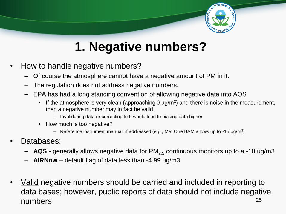
1. Negative numbers?

• How to handle negative numbers?

– Of course the atmosphere cannot have a negative amount of PM in it.

– The regulation does not address negative numbers.

– EPA has had a long standing convention of allowing negative data into AQS

• If the atmosphere is very clean (approaching 0 µg/m3) and there is noise in the measurement,

then a negative number may in fact be valid.

– Invalidating data or correcting to 0 would lead to biasing data higher

• How much is too negative?

– Reference instrument manual, if addressed (e.g., Met One BAM allows up to -15 µg/m3)

• Databases:

– AQS - generally allows negative data for PM2.5 continuous monitors up to a -10 ug/m3

– AIRNow – default flag of data less than -4.99 ug/m3

• Valid negative numbers should be carried and included in reporting to

data bases; however, public reports of data should not include negative

numbers 25

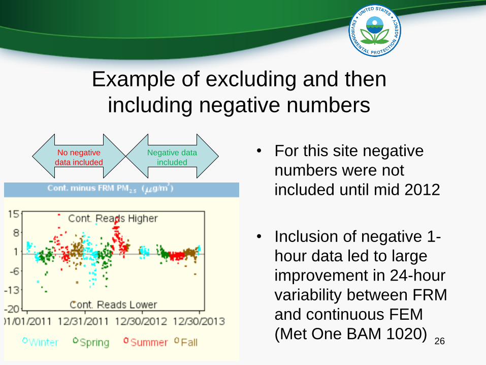
Example of excluding and then

including negative numbers

• For this site negative

numbers were not

included until mid 2012

• Inclusion of negative 1-

hour data led to large

improvement in 24-hour

variability between FRM

and continuous FEM

(Met One BAM 1020)26

No negative

data included

Negative data

included

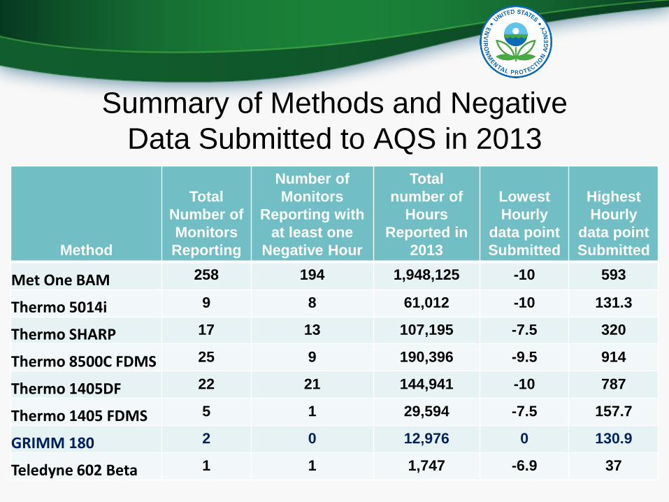
Summary of Methods and Negative

Data Submitted to AQS in 2013

27

Method

Total

Number of

Monitors

Reporting

Number of

Monitors

Reporting with

at least one

Negative Hour

Total

number of

Hours

Reported in

2013

Lowest

Hourly

data point

Submitted

Highest

Hourly

data point

Submitted

Met One BAM 258 194 1,948,125 -10 593

Thermo 5014i 9 8 61,012 -10 131.3

Thermo SHARP 17 13 107,195 -7.5 320

Thermo 8500C FDMS 25 9 190,396 -9.5 914

Thermo 1405DF 22 21 144,941 -10 787

Thermo 1405 FDMS 5 1 29,594 -7.5 157.7

GRIMM 180 2 0 12,976 0 130.9

Teledyne 602 Beta 1 1 1,747 -6.9 37

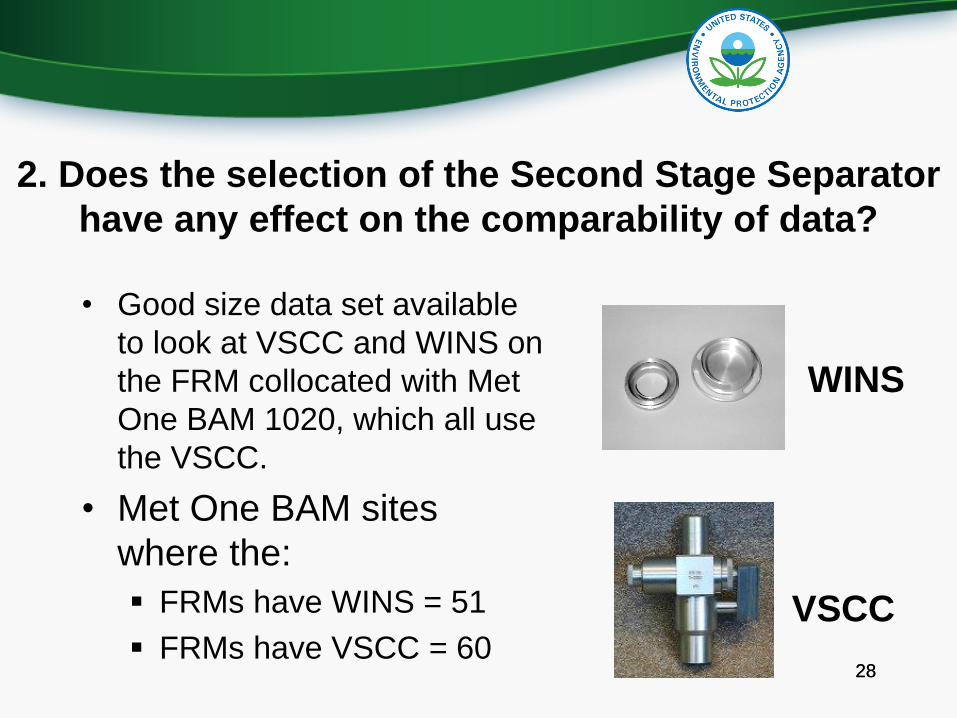
2. Does the selection of the Second Stage Separator

have any effect on the comparability of data?

• Good size data set available

to look at VSCC and WINS on

the FRM collocated with Met

One BAM 1020, which all use

the VSCC.

• Met One BAM sites

where the:

FRMs have WINS = 51

FRMs have VSCC = 602828

VSCC

WINS

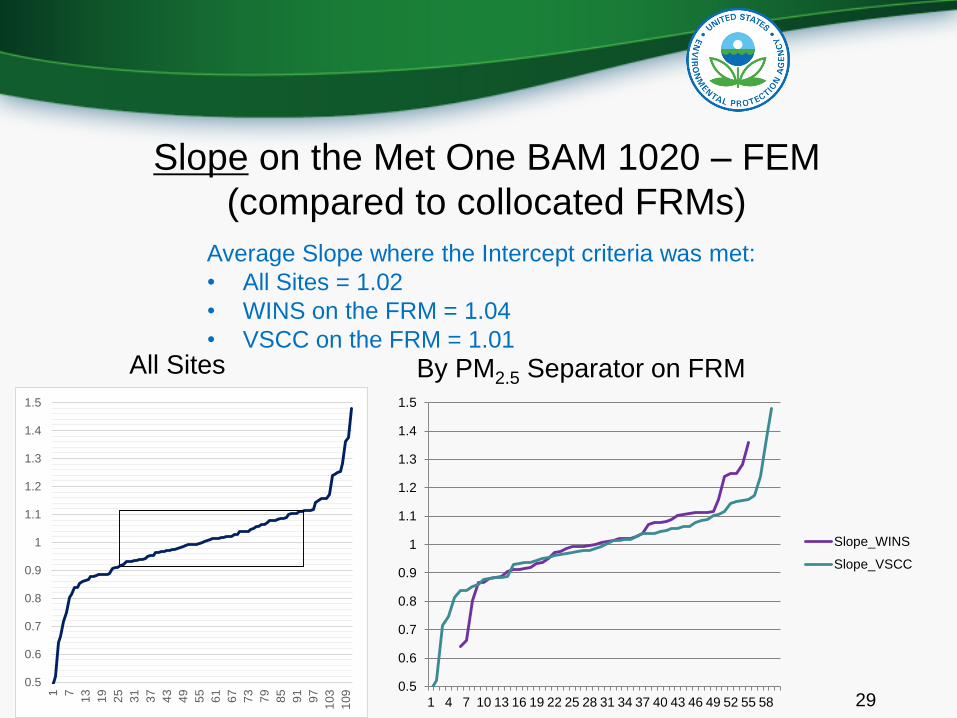
Slope on the Met One BAM 1020 – FEM


290.5

0.6

0.7

0.8

0.9

1

1.1

1.2

1.3

1.4

1.5

1 7

13

19

25

31

37

43

49

55

61

67

73

79

85

91

97

103

109 0.5

0.6

0.7

0.8

0.9

1

1.1

1.2

1.3

1.4

1.5

1 4 7 10 13 16 19 22 25 28 31 34 37 40 43 46 49 52 55 58

Slope_WINS

Slope_VSCC

All Sites By PM2.5 Separator on FRM

Average Slope where the Intercept criteria was met:

• All Sites = 1.02

• WINS on the FRM = 1.04

• VSCC on the FRM = 1.01

30-3

-2

-1

0

1

2

3

4

5

6

1 4 7 101316192225283134374043464952555861

Intercept_WINS

Intercept_VSCC

-3

-2

-1

0

1

2

3

4

5

6

1 6

11

16

21

26

31

36

41

46

51

56

61

66

71

76

81

86

91

96

101

106

111

Intercept on the Met One BAM 1020 – FEM


All Sites By PM2.5 Separator on FRM

Average Intercept where the slope criteria was met:

• All Sites = 1.14

• WINS on the FRM = 1.11

• VSCC on the FRM = 1.15

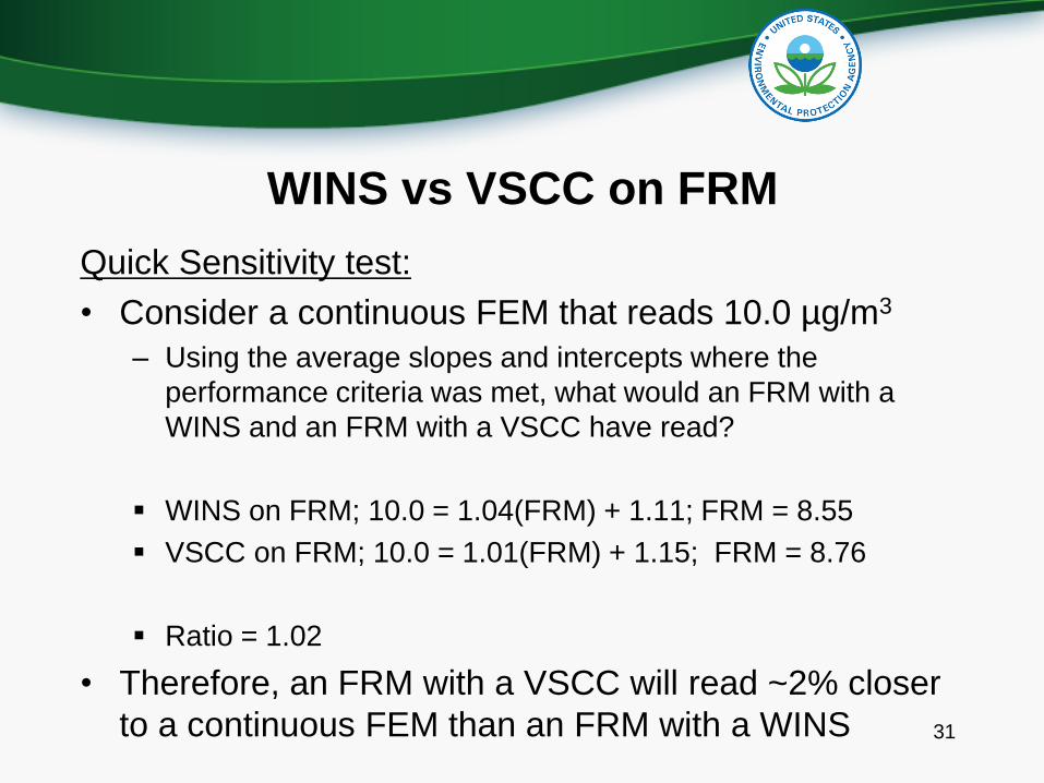
WINS vs VSCC on FRM

Quick Sensitivity test:

• Consider a continuous FEM that reads 10.0 µg/m3

– Using the average slopes and intercepts where the

performance criteria was met, what would an FRM with a

WINS and an FRM with a VSCC have read?

WINS on FRM; 10.0 = 1.04(FRM) + 1.11; FRM = 8.55

VSCC on FRM; 10.0 = 1.01(FRM) + 1.15; FRM = 8.76

Ratio = 1.02

• Therefore, an FRM with a VSCC will read ~2% closer

to a continuous FEM than an FRM with a WINS 31

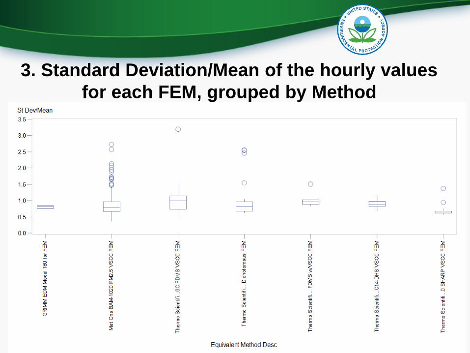
3. Standard Deviation/Mean of the hourly values

for each FEM, grouped by Method

32

Assessing the Data - Summary

Ensure you have good FRM data

Use Assessments to evaluate the comparability of

your data

Methods can meet expected performance criteria, but

much work remains

Negative numbers matter and should be reported

when valid (noise near zero)

Sites that use a VSCC on the FRM tend to have

slightly better comparability to the Met One BAM than

sites with a WINS on the FRM33

pm2.5 continuous monitoring assessing the data · pm 2.5 continuous monitoring assessing the data...

Documents