PM2.5 & Secondary PM2.5

Analysis for PSD

Permitting: A Case Study in

Missouri

March, 2015

Sarah Teefey

Presentation Overview

˃ PM2.5 Background

˃ EPA Guidance for PM2.5 Permit

Modeling

˃ Case Study

Part 1: Identifying a Representative

PM2.5 Monitor

Part 2: Quantifying Secondary PM2.5 as

part of Demonstrating Compliance

with NAAQS & PSD Increments

PM2.5 Background ˃ PM2.5

Particulate matter less than 2.5

micrometers in diameter.

˃ Primary PM2.5

PM2.5 emitted directly from a

source.

˃ Secondary PM2.5

PM2.5 formed from the chemical

reaction of precursor pollutants

emitted from a source

downwind of the original

pollution source.

♦ Precursors include NOx and SO2

PM2.5 Background

˃ First NAAQS for PM2.5 was established in 1997.

˃ EPA allowed PM10 to serve as surrogate for

PM2.5 in PSD BACT and air quality analysis

until May 2011.

Since May 2011, PM2.5 must be considered on its

own.

Challenge since has been how to account for the

secondary piece.

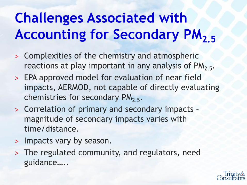
Challenges Associated with

Accounting for Secondary PM2.5

˃ Complexities of the chemistry and atmospheric

reactions at play important in any analysis of PM2.5.

˃ EPA approved model for evaluation of near field

impacts, AERMOD, not capable of directly evaluating

chemistries for secondary PM2.5.

˃ Correlation of primary and secondary impacts –

magnitude of secondary impacts varies with

time/distance.

˃ Impacts vary by season.

˃ The regulated community, and regulators, need

guidance…..

EPA & PM2.5

˃ New EPA Guidance: “Guidance for PM2.5

Permit Modeling” from May 2014 ♦ Emphasis on secondary PM2.5

♦ Cannot use AERMOD to simulate secondary PM2.5

– “The accounting for precursor emissions impact on

secondary PM2.5 formation may be: a) qualitative in

nature; b) based on a hybrid of qualitative and

quantitative assessments utilizing existing technical

work; or c) a full quantitative photochemical grid

modeling exercise.”

EPA May 2014 Guidance Summary

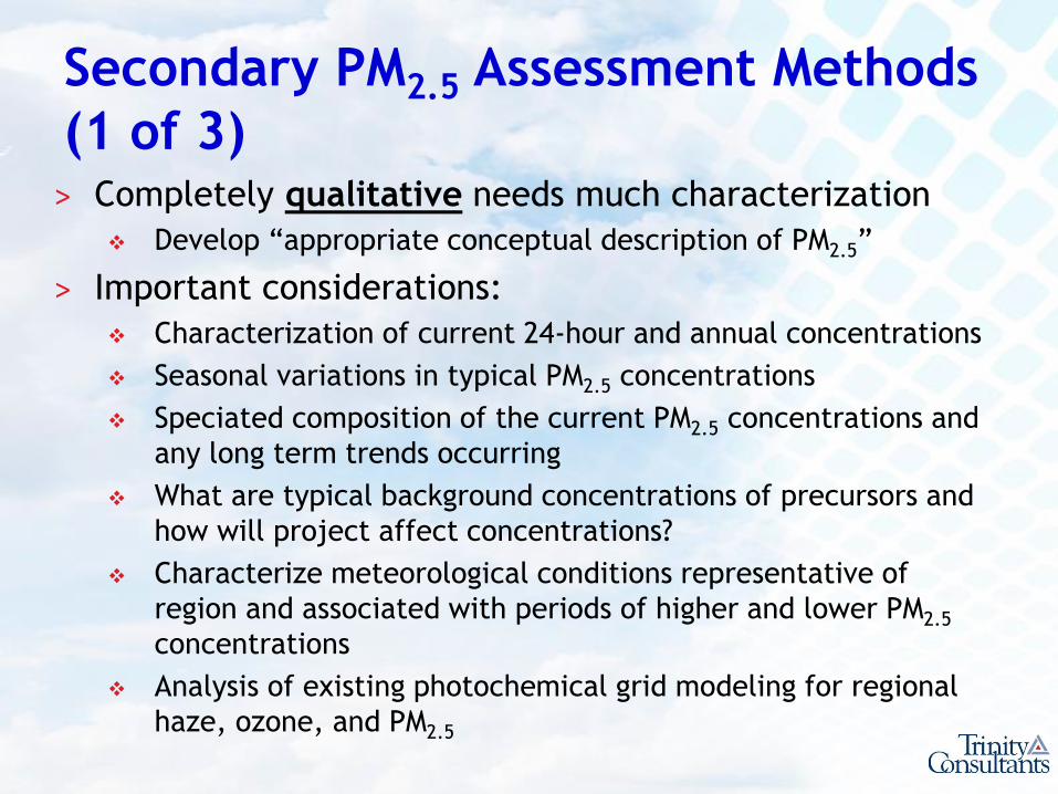
Secondary PM2.5 Assessment Methods

(1 of 3) ˃ Completely qualitative needs much characterization

Develop “appropriate conceptual description of PM2.5”

˃ Important considerations:

Characterization of current 24-hour and annual concentrations

Seasonal variations in typical PM2.5 concentrations

Speciated composition of the current PM2.5 concentrations and

any long term trends occurring

What are typical background concentrations of precursors and

how will project affect concentrations?

Characterize meteorological conditions representative of

region and associated with periods of higher and lower PM2.5

concentrations

Analysis of existing photochemical grid modeling for regional

haze, ozone, and PM2.5

Secondary PM2.5 Assessment Methods

(2 of 3)

˃ Hybrid qualitative/quantitative approach

Some quantification of secondary PM2.5 may be need to

show source will not contribute to violation of NAAQS.

Add analysis of local/region specific “offset ratios” for

precursor emissions (i.e. how readily the precursors form

the fine particles in the modeled domain)

This approach may include a modeled “overlay” of direct

PM2.5 and a simplified approach for assessing the

secondary formation

˃ EPA recommends consultation with Regional Office –

applicants should work diligently with the permitting

authority through the modeling protocol process

Secondary PM2.5 Assessment Methods

(3 of 3)

˃ Quantitative approach

Photochemical Model (e.g., CAMx or CMAQ)

Only expected to be needed in “rare” cases

Very expensive and time consuming

Requires EPA Region and EPA Headquarters approval

Chemistry Plume Models? (e.g., SCICHEM, updated CALPUFF)

Since May 2014 Guidance, What

are States Doing?

˃ Some States have already been requiring, and will continue to require, hybrid approach type assessments for secondary PM2.5.

˃ Some States looking for guidance on what can justify qualitative versus hybrid versus quantitative.

˃ A common theme: case by case assessment. State requirements regarding secondary PM2.5 will be a

constantly changing and evolving theme over the coming years.

The analysis your facility may have been allowed to do in one State, may not be acceptable (or desired) in another State.

May 2014 Guidance Summary – Case

Study Approach Determination

May 2014 Guidance Summary – Case

Study Approach Determination

Project Overview

˃ PSD permit required PM2.5, NOx and SO2 greater than SER

˃ Regulations have vacated PM2.5 SMC (Significant Monitoring Concentration) so any increase over SER warrants review of existing concentrations Conduct site specific monitoring

Find a representative PM2.5 data from existing monitor

– Represents concentrations surrounding proposed facility

– Can be used to derive a “clean” background concentration

PSD = Modeled PM2.5 + Secondary PM2.5 + Background

– Data from the monitor can also be used in qualitative/quantitative analysis

A Case Study - Part 1

Identifying a Representative

PM2.5 Monitor

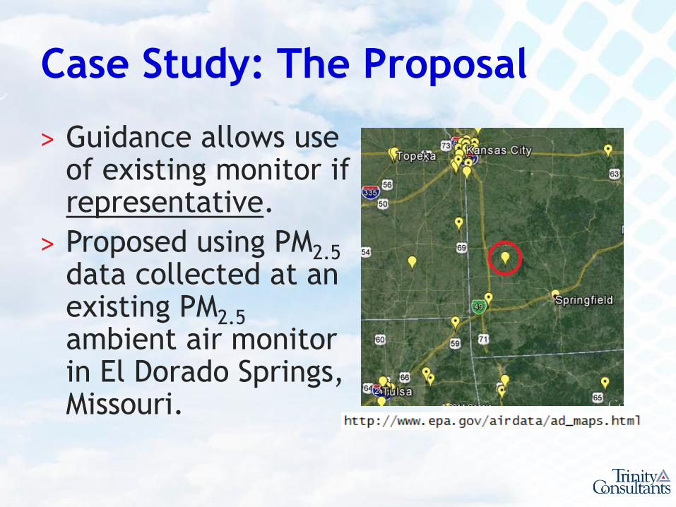
Case Study: The Proposal

˃ Guidance allows use of existing monitor if representative.

˃ Proposed using PM2.5 data collected at an existing PM2.5 ambient air monitor in El Dorado Springs, Missouri.

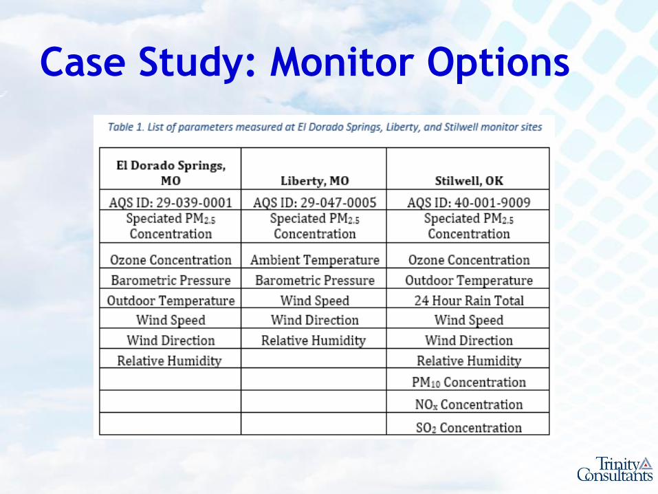
Case Study: Monitor Options

˃ Located all PM2.5

monitors near

facility.

˃ Narrowed options

based on:

Data currentness

Data quality

Speciation of PM2.5

Meteorological

conditions in region

Case Study: Monitor Options ˃ Why are speciated monitors preferred?

Characterize chemical composition of the PM2.5

Can evaluate PM in the form of nitrates,

sulfates and ammonia

0

5

10

15

20

25

30

35

40

45

50

2011 2012 2013

% o

f To

tal S

pec

iate

d P

M2.

5

Nitrates Sulfates Ammonia Other

Case Study: Monitor Options

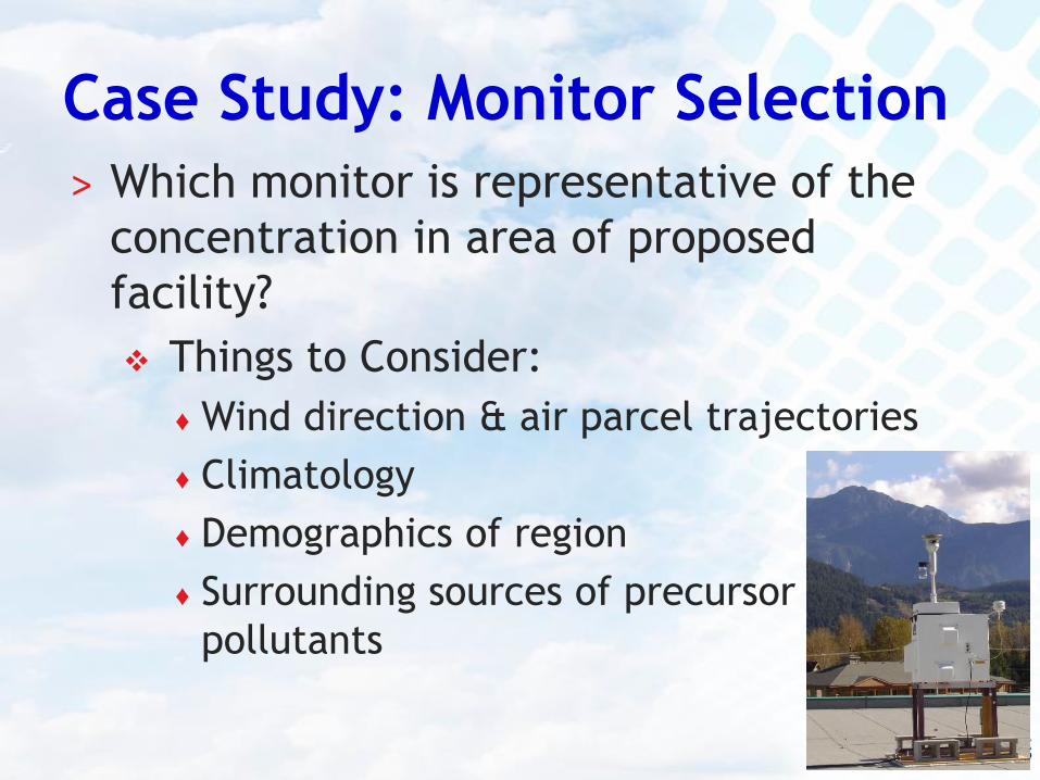
Case Study: Monitor Selection

˃ Which monitor is representative of the

concentration in area of proposed

facility?

Things to Consider:

♦ Wind direction & air parcel trajectories

♦ Climatology

♦ Demographics of region

♦ Surrounding sources of precursor

pollutants

Case Study: Wind Analysis ˃ Determine average wind speed and

direction near proposed facility location

5 year analysis for 3 nearby airports

Case Study: Wind Analysis ˃ Narrowed data by putting emphasis on

winter season months

Cooler temperatures are more ideal for nitrate

formation and thus, secondary PM2.5

formation.

Wind roses using data from October – March for

5 years.

Case Study: Wind Analysis

˃ Joplin Airport closest weather station to facility

˃ 20% of time analyzed had wind direction between 170º (S) and 200º (SSW)

˃ Grove & Monett - more variation Stronger SSE and NW

components

Case Study: Forward Trajectories

˃ Demonstrates path air parcel took from a point of origin.

˃ Used NOAA’s HYSPLIT Model.

˃ Image of December 2013 trajectories.

˃ 13% (4 days) air advected within 17º sector of El Dorado Springs monitor.

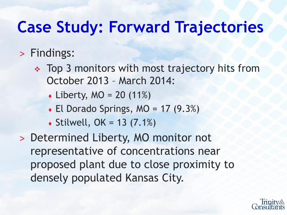
Case Study: Forward Trajectories

˃ Findings:

Top 3 monitors with most trajectory hits from

October 2013 – March 2014:

♦ Liberty, MO = 20 (11%)

♦ El Dorado Springs, MO = 17 (9.3%)

♦ Stilwell, OK = 13 (7.1%)

˃ Determined Liberty, MO monitor not

representative of concentrations near

proposed plant due to close proximity to

densely populated Kansas City.

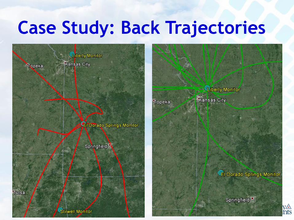
Case Study: Back Trajectories ˃ Demonstrates path air parcels have taken prior

to arriving at monitor site.

˃ Again used NOAA’s HYSPLIT (Hybrid Single

Particle Lagrangian Integrated Trajectory

Model).

˃ Only used cold season days when the monitor

showed exceedance of 12 µg/m3 (annual

NAAQS primary PM2.5 standard)

Information from EPA Air Quality website

El Dorado Springs = 8 exceedances, 0 hits within 10 km

Liberty = 17 exceedances, 1 hit

Stilwell = 10 exceedances, 0 hits

Case Study: Back Trajectories

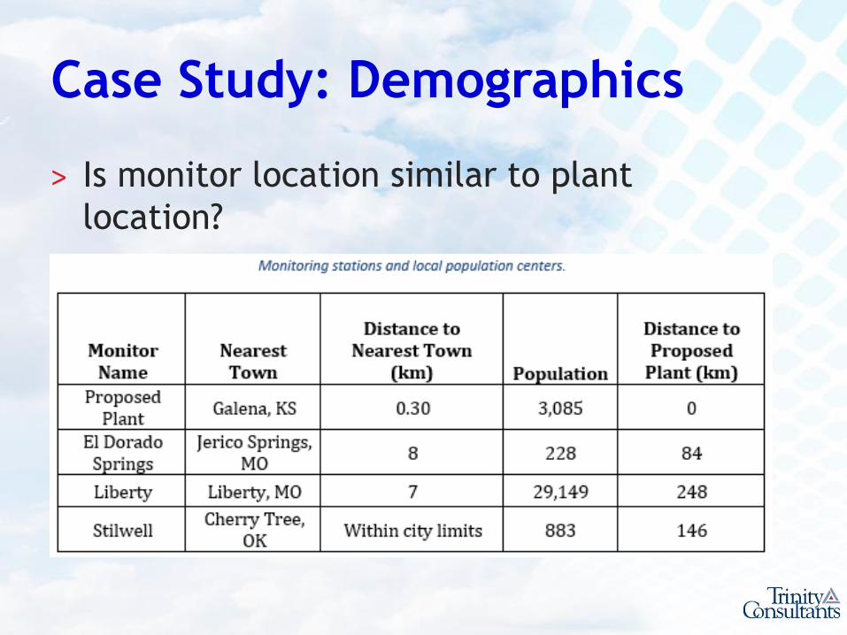
Case Study: Demographics

˃ Is monitor location similar to plant

location?

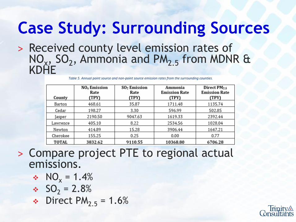
Case Study: Surrounding Sources ˃ Received county level emission rates of

NOx, SO2, Ammonia and PM2.5 from MDNR & KDHE

˃ Compare project PTE to regional actual emissions. NOx = 1.4%

SO2 = 2.8%

Direct PM2.5 = 1.6%

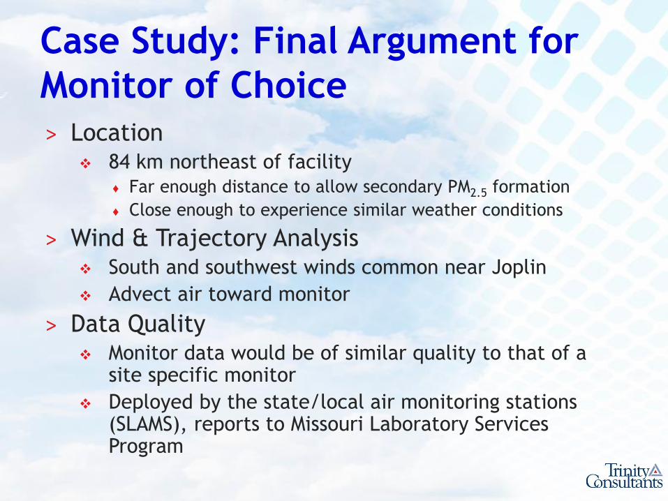
Case Study: Final Argument for

Monitor of Choice ˃ Location

84 km northeast of facility ♦ Far enough distance to allow secondary PM2.5 formation

♦ Close enough to experience similar weather conditions

˃ Wind & Trajectory Analysis South and southwest winds common near Joplin

Advect air toward monitor

˃ Data Quality Monitor data would be of similar quality to that of a

site specific monitor

Deployed by the state/local air monitoring stations (SLAMS), reports to Missouri Laboratory Services Program

A Case Study - Part 2

Quantifying Secondary PM2.5 as

part of Demonstrating

Compliance with NAAQS & PSD

Increments

Case Study: How to Quantify

Secondary PM2.5

˃ AERMOD can only be used to find primary (direct)

PM2.5 emissions, not secondary PM2.5 emissions

˃ How to quantify secondary PM2.5 emissions?

Cross-State Air Pollution Rule (CSAPR)

Pollutant offset ratios suggested by the National

Association of Clean Air Agencies (NACAA) in May

2014 guidance

Case Study: Cross-State Air

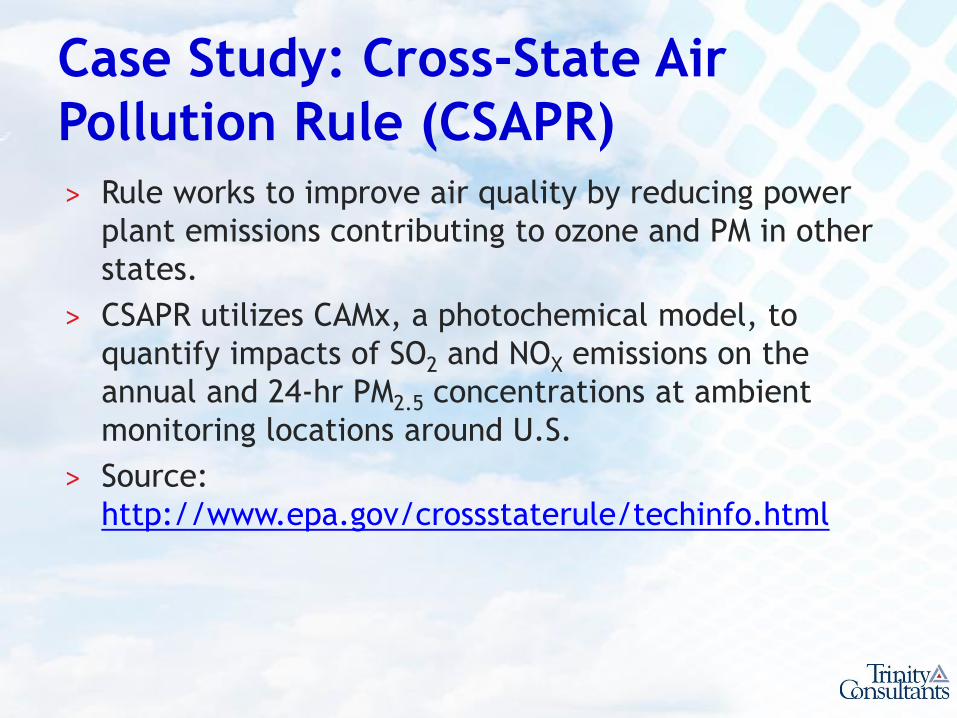
Pollution Rule (CSAPR)

˃ Rule works to improve air quality by reducing power

plant emissions contributing to ozone and PM in other

states.

˃ CSAPR utilizes CAMx, a photochemical model, to

quantify impacts of SO2 and NOX emissions on the

annual and 24-hr PM2.5 concentrations at ambient

monitoring locations around U.S.

˃ Source:

http://www.epa.gov/crossstaterule/techinfo.html

Case Study: Cross-State Air

Pollution Rule (CSAPR)

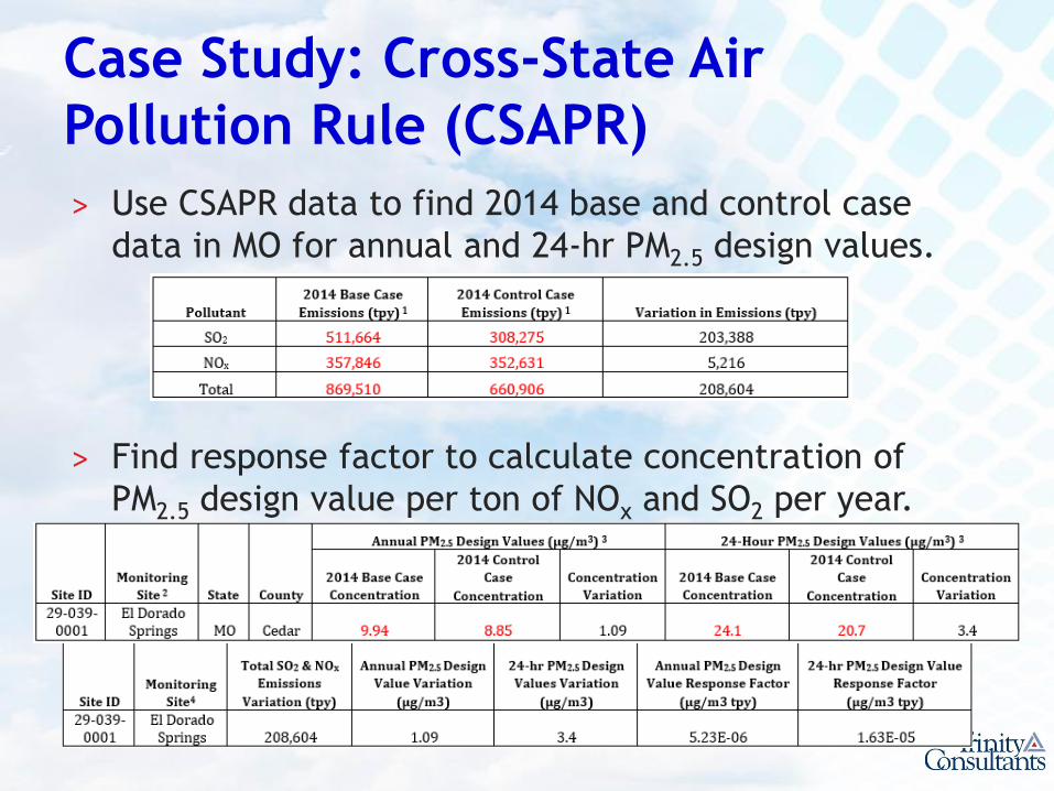
˃ Use CSAPR data to find 2014 base and control case

data in MO for annual and 24-hr PM2.5 design values.

˃ Find response factor to calculate concentration of

PM2.5 design value per ton of NOx and SO2 per year.

Case Study: Cross-State Air

Pollution Rule (CSAPR)

˃ The response factor was multiplied by the

proposed project’s total SO2 and NOx PTE values to

find estimated impact on secondary formation of

PM2.5 at monitor.

Case Study: Cross-State Air

Pollution Rule (CSAPR)

˃ Impacts of combined primary and secondary PM2.5

on NAAQS analysis.

Case Study: Pollutant Offset Ratio ˃ Guidance provided by the NACAA: Finds estimate

of emission rate

Pollutant offset ratios of 40:1 for SO2 and 200:1 for

NOx

Secondary PM2.5 Emissions =𝑁𝑂𝑥 𝑡𝑝𝑦

200+

𝑆𝑂2 𝑡𝑝𝑦

40

Result = 1.49 lb/hr of secondary PM2.5

Use screening model (SCREEN3) to assess downwind

impact of emission rate

♦ Enter stack information, meteorology and terrain options

♦ Does not account for chemical reactions in formation of PM2.5

just gives estimate of downwind concentration.

♦ Result = 2.93 µg/m3 approximately 2,506 m from source.

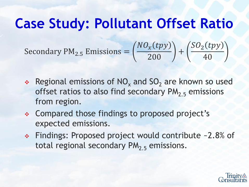
Case Study: Pollutant Offset Ratio

Secondary PM2.5 Emissions =𝑁𝑂𝑥 𝑡𝑝𝑦

200+

𝑆𝑂2 𝑡𝑝𝑦

40

Regional emissions of NOx and SO2 are known so used

offset ratios to also find secondary PM2.5 emissions

from region.

Compared those findings to proposed project’s

expected emissions.

Findings: Proposed project would contribute ~2.8% of

total regional secondary PM2.5 emissions.

Case Study: Secondary PM2.5 Analysis

for PSD Permit Conclusions

˃ Using both CSAPR and Pollutant Offset Ratio methods showed low amounts of secondary PM2.5 formed from NOx and SO2

˃ Maximum impacts from primary and secondary PM2.5 would not occur at same time & location, unlikely secondary PM2.5 would result in violation of NAAQS

˃ Compared secondary PM2.5 value found from pollutant offset ratios to regional values obtained from MDNR Our facility contributes about 3% to the total

regional value

Case Study: Feedback from

Agency

˃ This type of analysis is only the second of its

kind to be submitted to the state of Missouri.

˃ First was also a Trinity project submitted

several months before this one.

˃ MDNR had “95% approved” the similar analysis.

Questions?

Sarah Teefey

steefey@trinityconsultants.com Phone: 913-894-4500