pmod workflow for dosimetry · pdf filepmod workflow for dosimetry preprocessing 2...
TRANSCRIPT

Printed on 20 December, 2016
User's Guide
PMOD Workflow for Dosimetry Preprocessing
(PBAS, PKIN)
Version 3.8

i
Contents
Workflow for Dosimetry Preprocessing 2
Introduction ...................................................................................................................................................... 2 Conventions ..................................................................................................................................................... 4
Data Preparation in PBAS 5
Merge Frames Tool .......................................................................................................................................... 5 Decay Correction ............................................................................................................................................. 7 Timing Vector .................................................................................................................................................. 8 Inspection of Dynamic Series ......................................................................................................................... 9
VOI Definition in PBAS/Fuse It 10
VOI Properties ............................................................................................................................................... 10 Dosimetry Organ List ................................................................................................................................... 12
Residence Times Calculation in PKIN 16
Time-Activity Curve Transfer ...................................................................................................................... 17 Edit Patient ..................................................................................................................................................... 18 Edit Data ......................................................................................................................................................... 18 Operational Equations .................................................................................................................................. 19 Model Input Parameters ............................................................................................................................... 20 Model Output Parameters ............................................................................................................................ 21 OLINDA Case File Export ............................................................................................................................ 23
References 27
PMOD Copyright Notice 28
Index 29

PMOD Workflow for Dosimetry Preprocessing 2
Introduction
The estimation of the internal radiation dose in nuclear medicine is a common requirement
for novel radiotracers. The ‘Effective Dose’ to the patient or volunteer, in milli-Sieverts per
mega-Bequerel (mSv/MBq) of radiotracer administered, and identification of the ‘dose-
limiting organs’, may be required by Ethical Commissions before the maximum injectable
dose can be defined. Calculation of such radiation dose is commonly known as ‘dosimetry’.
Prior to studies in humans, dosimetry in animals can be extrapolated to provide an initial
estimate of ‘Effective Dose’. The total number of disintegrations in the organs during the
presence of the radionuclide in the body is required. In order to calculate the total number of
disintegrations in each organ, knowledge of the radiotracer pharmacokinetics is required.
Although ex vivo biodistribution studies are still performed in animals, PET and SPECT
imaging allow the tracer kinetics to be quantified in single subjects, reducing the number of
animals required and making human studies possible. However, accurately estimating the
tracer kinetics throughout the time that the radioisotope is present in the body typically
requires a substantially different protocol to that normally used in dynamic PET/SPECT.
According to International Commission on Radiation Units and Measurements report no 67
[1, 2], image acquisition starting times of 1/3, 2/3, 3/2, 3, and 5 multiples of the effective half
life are recommended to sufficiently describe the kinetics. In the case of radionuclides with
longer half lives, even F-18, this necessitates multiple scanning sessions.
Deriving time-activity curves from such data thus necessitates merging of the independent
scan sessions into a dynamic series, with careful consideration of decay correction. In fact, as
the total number of disintegrations in each organ is required, no decay correction should be
applied to imaging data used for dosimetry. However, as decay correction to the acquisition
start time is the default in clinical imaging, particularly for whole body PET with multiple
fields-of-view, a pragmatic approach is to ensure that decay correction to a common time
point is applied to all scans. From this starting point, decay according to the known
radionuclide half-life can be applied.
The activity in each organ at each time point can be extracted from the imaging data using
volume-of-interest (VOI)-based analysis. Note that due to scanning in independent sessions,
these VOIs may need to adapt to changing organ positions over time (dynamic VOIs).
Once the tracer kinetics in each organ are known, the total number of disintegrations during
the presence of the radionuclide can be calculated as the area-under-the-curve (AUC; y-axis:
total activity in Bq in organ, x-axis: time in hours). Extension from the last data point
collected to infinity (or decay of the last Bq in the body) is usually achieved by analytic
integration based on the known radionuclide half-life. The total number of disintegrations is
known as the ‘residence time’, and has the units ‘Bequerel hour per Bequerel’. A number of
methods have been proposed to calculate the residence time, ranging from simple
rectangular or trapezoidal calculation of the AUC for the measured data portion, to fitting of
exponential models and analytical calculation of AUC from injection to infinity.
Workflow for Dosimetry Preprocessing

PMOD Workflow for Dosimetry Preprocessing 3
These residence times are used as the input to digital ‘phantoms’, representing a standard
model of adult male or female, within which the dose from each source region to all other
target regions can be calculated (see [3]). These calculations are performed in standalone
software tools, such as OLINDA/EXM [4] and IDAC [5]. The output of these programs is a
table containing individual doses in mSv per organ per MBq injected, and the Effective Dose,
a weighted average between critical organs (e.g. ICRP publication 60, 1991 [6]).
The recommendations for dosimetry are evaluated by the International Commission on
Radiological Protection (ICRP; www.icrp.org ), and updated at regular intervals. Recently,
ICRP publication 103 updated the weighting factors for calculation of the Effective Dose, and
introduced more sophisticated voxelized phantoms [7]. ICRP publication 89 updated the
organ masses used in the calculation of residence times, and introduced reference values for
both males and females of six different ages [8].
PMOD supports a tailored workflow of preprocessing steps to arrive at reliable dosimetry
input data from a set of sequential image acquisitions, using the base tool PBAS and the
kinetic modeling tool PKIN.

PMOD Workflow for Dosimetry Preprocessing 4
Conventions
Please note the conventions used in this documentation:
Mouse Operation Type of Information
Click The term click in the text means that the left mouse button is pressed
down and then released. Clicking with another mouse button is
indicated by a description such as right click.
Double-click The term double-click means that the left mouse button is clicked twice
in a fast sequence without moving the mouse.
Drag The term drag means that the left mouse button is pressed and held
down while the mouse is moved.
Formatting Type of Information
Special Bold Items you must select in the user interface of the program, such as
menu options, command buttons, or items in a list.
Emphasis Used to emphasize the importance of a point or for variable
expressions such as parameters.
CAPITALS Names of keys on the keyboard. For example, SHIFT, CTRL, or ALT.
KEY+KEY Key combinations for which you must press and hold down one key
and then press another, for example, CTRL+P, or ALT+F4.
Please refer to the Glossary at the end of this document for information regarding
specialized terms used in the documentation.

PMOD Workflow for Dosimetry Preprocessing 5
The images of multiple studies may be separated by hours or even days depending on the
half-life of the isotope in question. The first task is to combine those images into a consistent
dynamic series. A crucial element during data merging is the proper handling of decay
correction for independently acquired series. For image formats containing sufficient header
information (e.g. DICOM), PMOD’s Merge tool can derive the series timing directly from the
image headers and offers decay correction at the individual image and dynamic series levels.
Merge Frames Tool
The Merge Frames tool is available on the View page of the VIEW module, below the main
image controls. It is activated once multiple image series are loaded.
Data Preparation in PBAS

PMOD Workflow for Dosimetry Preprocessing 6
The Merge Frames tool allows the combination of image series with the same geometry into
a joint dynamic series. Static and dynamic series may be merged.
Activating Merge Frames opens a dialog window as illustrated below. The list in the upper
left shows the loaded image series in loading order. The list in the upper right shows the
image series that will be combined into a dynamic series with the current sorting order.
Initially, all series appear in the original order. The options related to applying decay
correction during merging and generating the timing of the new dynamic series is located in
the lower part.
Series can be copied from left to right by Double-Clicking in the left list, or selecting a list
element and activating the arrow between the lists. The double arrow copies all loaded series
to the right.
The order of the Selected for Merge list can be modified by selecting a list element and
adjusting its position in the list using the arrows to the right.

PMOD Workflow for Dosimetry Preprocessing 7
If the columns contain information that is suitable for sorting, the sorting button AZ can be
enabled and sorting started by clicking the appropriate column header. In the example
above, the acquisition time was used to sort the static series into the proper acquisition
order.
Decay Correction
When joining PET or SPECT data into a dynamic series, a consistent decay correction must
be ensured. Usually, each image series is corrected to its own acquisition start time.
Therefore, when joining static series into a dynamic series, later series have to be decay
corrected to the start of the first acquisition by scaling them by a corresponding factor. The
appropriate setting for this situation is to enable Decay Correction, confirm that Source data
is decay corrected, check that the isotope Half Time is correct, and check that the
Acquisition Start times of the series Selected for Merge are sorted correctly, as illustrated
below. The Acquisition Start time of the first series in the list is taken as the common time for
decay correction.
Alternatively, if the time of tracer injection varies from the start of acquisition, and this has
been correctly recorded in the image header, Correct to injection may be activated.
If image acquisition timing data is not available in the image header, it is recommended that
the user resave their data in a format that allows the timing information to be added (e.g.
DICOM), before using the Merge Frames tool.

PMOD Workflow for Dosimetry Preprocessing 8
Timing Vector
The timing of the created dynamic series must be constructed. It can be specified using the
Create time vector based on selection.
Processing is started with the Merge button, and the user has a choice between replacing the
currently open image series, or creating a new series.
Before the new series is created and optionally decay corrected, the timing is displayed in a
dialog window for confirmation and editing. In the example below, which was generated
using frames acquisition times, there are gaps of about 40 seconds between the acquisitions.
They occurred because the scanner had to be restarted for the subsequent whole-body
acquisitions. Using frames duration, this information would have been missed.

PMOD Workflow for Dosimetry Preprocessing 9
Inspection of Dynamic Series
Once merging is complete, the user should examine the resulting dynamic series. By default,
the suffix [MERGE_T] is added to the Series Description. This can be edited using the Info &
Edit dialog window available with the button, then Edit Patient / Study Info.
Of particular importance for later residence time calculation is the injected dose of
radiotracer and radionuclide half-life. These parameters can be edited on the SUV
PARAMETERS tab. Note, the new dynamic image series must be saved in a suitable image
format to maintain this information in the image header (e.g. DICOM). Radionuclide and
Calibrated dose in syringe are used during the calculation of residence times in PKIN, and
are written to the exported OLINDA .cas file. However, note that OLINDA does not
interpret this information during loading.
Additionally, the user should check the image for movement between frames. This is
particularly important where multiple scanning sessions were used, as positioning of the
subject is very likely to change. The presence of movement or misalignment between organ
positions across time influences the type of VOIs required in the next step.

PMOD Workflow for Dosimetry Preprocessing 10
As a next step organ outlines (VOIs) need to be defined. PMOD offers various flexible
approaches to overcome the challenges of this task. Organs with clear uptake can be
addressed via iso-contouring. Others may require manual or semi-automatic outlining, or
recourse to a matched anatomical data set. Thanks to the 4D-capabilites of PMOD VOIs,
organ position and even shape changes between sequential acquisitions can be precisely
tracked. Finally, using a drop-down list, each VOI can easily be assigned to an organ with
properties corresponding to a particular dosimetry phantom anatomy.
The basics of VOI analysis and descriptions of the tools available are available in a dedicated
section of the PMOD online manual: http://doc.pmod.com/pbas/640.htm, and are thus not
covered in detail here. The relevant aspects of VOI Properties are described below.
VOI Properties
In the case of many organs and tissues required for dosimetry analysis it is not possible to
make a complete delineation, because the organ/tissue is not clearly visible, or because (as in
the case of muscle), it is not compact. In this case, standard organ volumes can be used in
order to extrapolate VOI uptake to organ uptake. An organ can be assigned to a defined VOI
as illustrated below:
1) Select the VOI in the list.
2) Open the VOI properties editor using the button, and select the Set button.
3) Select an appropriate name list. For instance, the OLINDA (Adult male) contains
the organ definitions (name, volume, mass) for the adult male phantom in OLINDA.
4) Choose the organ from the list. The predefined ORGAN volume and mass are
shown and may be edited.
5) Close with the Set VOI name and color button.
An additional advantage of this workflow is that the VOI names correspond exactly to those
required for export of an OLINDA/EXM case file at the end of the overall dosimetry analysis.
VOI Definition in PBAS/Fuse It

PMOD Workflow for Dosimetry Preprocessing 11
In the event of body/organ movement between frames, a dynamic (4D) VOI may be
necessary. An initial VOI should be created, typically on the first time frame, then the VOI
Properties should be set to Dynamic.

PMOD Workflow for Dosimetry Preprocessing 12
Static VOI : If a VOI is static, the same VOI definition is applied and shown at all times.
Dynamic VOI : For dynamic VOIs, a different VOI definition can be used at different
times. Note that a dynamic VOI is only shown when viewing the images of the time frame it
was defined on. As long as only one VOI is defined, statistics calculation will apply this VOI
at all times as with a static VOI. However, as soon as VOIs have been defined at more than
one time, it is required that VOIs are defined at all times. Here the VOI propagate
functionality may be helpful (available on the VOI Adjustment tool bar).
Propagate option button : Propagation for VOIs means copying a VOI from one time
frame to another. This function is only available for dynamic series and VOIs set to dynamic
in VOI Properties.
Dosimetry Organ List
Organs available in the OLINDA (Adult male), with default mass and volume, are listed
below:
OLINDA (Adult male) Organ volume (ml) Organ mass (g)
Adrenals 15.52380952 16.3
Brain 1352.380952 1420.0
Breasts_including_skin NA NA

PMOD Workflow for Dosimetry Preprocessing 13
Gallbladder_contents 53.04761905 55.7
LLI_contents 136.1904762 143.0
SI_contents 1047.619048 1100.0
Stomach_contents 247.6190476 260.0
ULI_contents 220.952381 232.0
Heart_contents 432.3809524 454.0
Heart_wall 300.952381 316.0
Kidneys 284.7619048 299.0
Liver 1819.047619 1910.0
Lungs* 952.3809524 1000.0
Muscle 26923.0 28000.0
Ovaries NA NA
Pancreas 89.80952381 94.3
Red_marrow 1066.666667 1120.0
Cortical_bone 3809.52381 4000.0
Trabecular_bone 952.3809524 1000.0
Spleen 174.2857143 183.0
Testes 37.23809524 39.1
Thymus 19.9047619 20.9
Thyroid 19.71428571 20.7
Urinary_bladder_contents 200.952381 211.0
Uterus NA NA
Fetus NA NA
Placenta NA NA
Organ masses were taken from Stabin & Siegel (2003) [3]. Note: a tissue density of 1.05 g/ml
was assumed for conversion of all organ masses to volume. Users may choose to use the
lower density of 0.4 g/ml for lung.

PMOD Workflow for Dosimetry Preprocessing 14
Organs available in the OLINDA (Adult female), with default mass and volume, are listed
below:
OLINDA (Adult female) Organ volume (ml) Organ mass (g)
Adrenals 13.33 14.0
Brain 1142.86 1200.0
Breasts_including_skin 392.38 412.0
Gallbladder_contents 47.62 50.0
LLI_contents 128.57 135.0
SI_contents 357.14 375.0
Stomach_contents 219.05 230.0
ULI_contents 200.0 210.0
Heart_contents 390.48 410.0
Heart_wall 228.57 240.0
Kidneys 261.9 275.0
Liver 1333.33 1400.0
Lungs* 761.9 800.0
Muscle 16346.0 17000.0
Ovaries 10.48 11.0
Pancreas 80.95 85.0
Red_marrow 1000.0 1050.0
Cortical_bone 2857.14 3000.0
Trabecular_bone 714.29 750.0
Spleen 142.86 150.0
Testes NA NA
Thymus 19.05 20.0
Thyroid 16.19 17.0
Urinary_bladder_contents 152.38 160.0

PMOD Workflow for Dosimetry Preprocessing 15
Uterus 75.24 79.0
Fetus NA NA
Placenta NA NA

PMOD Workflow for Dosimetry Preprocessing 16
The radioactivity in each organ VOI is then averaged and transferred to PKIN, PMOD’s
kinetic modeling tool, as a time-activity curve (TAC). The TACs may feature time shifts to
account for acquisitions with multiple bed positions. Before the actual number of
disintegrations in the organs can be estimated, decay correction – if applied – has to be
undone, and activity concentration data needs to be converted into total organ uptake.
PMOD’s workflow allows this process to be automated. Several integration approaches can
be applied to the count rate curves generated: Discrete rectangular or trapezoidal integration
followed by isotope decay, fitting of the declining part of the data with exponentials and
algebraic integration, or a combination of both.
The OLINDA Residence Times model performs pre-processing steps for the calculation of
the absorbed dose from diagnostic or therapeutic radiopharmaceuticals. Given the time-
course of the activity in a volume of tissue, it calculates the Residence Time, which could in
fact better be called the Normalized Cumulated Activity [9] to avoid confusion of its
meaning. However, as it is widely used in literature, the notion Residence Time will be used
in the remainder of this section. The residence time represents the total number of
disintegrations occurring during an integration time, per unit of administered activity.
Ideally, integration is performed from the time of administration to infinity.
The organ residence times resulting from the OLINDA Residence Times model can serve as
input to a program such as OLINDA [4] for the actual calculation of the absorbed organ
doses.
Residence Times Calculation in PKIN

PMOD Workflow for Dosimetry Preprocessing 17
Time-Activity Curve Transfer
Following the definition of VOIs and assignment of VOI Properties as described in the
previous section, the tracer time-activity curves (TACs) for each organ are calculated using
the TAC Export button . The TAC Export dialog window is opened.
The TACs are displayed in the central curve display area, and their inclusion in the transfer
to PKIN can be toggled using the menu on the left.
Below the curve display area the time shift between actual acquisition of each organ can be
configured. Such a time shift can be used to correct for the acquisition of multiple fields-of-
view to create a whole body PET image.
Activating the Delay by VOI location button makes two options for time shift application
available.
Stop & Go is intended for data acquired with multiple fields-of-view. The number of table
positions used during whole body acquisition must be entered by the user, and the direction
of scanning defined by setting Time increases with slice number or Time decreases with
slice number (representing whether the subject was scanned from head to feet, or vice
versa). Once activated, the time shift for each organ is calculated and displayed in the curve
display area.
Continuous bed movement is applicable when the scanner supports whole body image
acquisition through a continuously moving bed, such as the Siemens Biograph mCT Flow.
To the right of the time-shift dialog, the Dosimetry model button enables automated
selection of the Residence Times model in PKIN following TAC transfer.
If decay correction was applied during merging, as described above, activation of Decay
correction to injection time is unnecessary.

PMOD Workflow for Dosimetry Preprocessing 18
Finally, the TACs can be transferred to PKIN using either Send (Set) or Send (Add) buttons.
Send (Add) will create a new tab if PKIN is already open.
Edit Patient
Depending on the method used to import the TACs into PKIN, isotope and activity
information may or may not be available. Radionuclide half-life and Calibrated dose in
syringe are necessary for residence time calculation. Transfer of TACs from VOI analysis in
another PMOD module will also transfer patient data including SUV information. Loading
of pre-saved TACs or TACs prepared as a text file will not include patient and SUV
information. These parameters can be edited in the Patient and Study Information window
as illustrated below. Activate Edit Patient in the Tools list, select SUV PARAMETERS, and
enter Radionuclide half-life and Pre-injected tracer activity. Note that the activity needs to
be calibrated to time 0 of the activity curve.
Edit Data
The regional VOI volume is available if the TAC was generated in PMOD's View tool and
transferred to PKIN.

PMOD Workflow for Dosimetry Preprocessing 19
An alternative approach is to edit the VOI and organ volumes as follows:
1) Activate Edit Data in the Tools list
2) Select a region in the upper list.
3) Choose Edit volume from the curve tools
4) Enter the Volume of the VOI in the dialog window.
5) Change The Organ Volume in the lower part. (currently, Organ mass is not used for
the calculation).
6) Close the PKIN data explorer with Ok.
Operational Equations
Given an activity A0 applied to a subject, and a measured (not decay corrected) activity A(t)
in an organ, the residence time t is calculated by
Note that the unit of t is usually given as [Bq×hr/Bq]. The measured part of the organ activity
can easily be numerically integrated by the trapezoidal rule. For the unknown remainder of
A(t) until infinity it is a conservative assumption to apply the radioactive decay of the
isotope. This exponential area can easily be calculated and added to the trapezoidal area.
Alternatively, if the measured activity curve has a dominant washout shape, a sum of
exponentials can be fitted to the to the measured data and the entire integral algebraically
calculated.

PMOD Workflow for Dosimetry Preprocessing 20
Model Input Parameters
The OLINDA Residence Times model in PKIN supports both the trapezoidal integration
approach as well as the use of fitted exponentials. It furthermore supports some practicalities
such as conversion of an average activity concentration in [kBq/cc] to activity in [Bq], by
multiplication with the VOI volume, and reversion of decay correction.
The OLINDA Residence Times model has 4 input parameters that need to be specified
interactively by the user. These settings can easily be propagated from one region to all
others with the Model & Par button.
Decay
corrected
Check this box if the loaded curves were decay corrected, as is usually the
case for PET imaging studies. The Halflife of the radioisotope will be used
to undo the decay correction.
Activity
concentration
Check this box if the loaded curves represent activity concentration, rather
than the total activity in a region. The volume of the region will be
multiplied with the signal to calculate activity in [Bq].
Isotope tail Check this box to use the radioactive decay shape for the integration from
the end of the last frame to infinity. This option is only relevant if
exponentials are fitted to the measurement.
For the Rectangle and Trapezoid methods it will always be enabled. For
the exponentials it will also be enabled if the exponential halftime is
longer than the isotope half-life (a warning will be recorded in the log).
Integration The integration method can be selected in the option list:

PMOD Workflow for Dosimetry Preprocessing 21
The Rectangle method is the natural selection for PET values that
represent the time average during the frame duration. If there are gaps
between the PET frames, the uncovered area is approximated by the
trapezoidal rule.
The Trapezoid method uses trapezoidal areas between the frame mid-
times.
With an Exponential selection, the specified number of decaying
exponentials is fitted to the measurements, and used for analytical
integration. Note that samples marked as invalid are neglected in the fit.
Exp integ from
0
Check this box to use the exponential from time zero for the integration. If
the box is unchecked, rectangular integration is used for samples before
Exp begin.
Exp begin Defines the time (frame mid), from which point onwards the exponentials
are fitted to the measurement.
Model Output Parameters
As soon as the Fit Region button is activated, the fits and calculations are performed,
resulting in a list of parameters:
Organ residence time
[Bq×hr/Bq]
Total number of disintegrations in the organ volume from
time 0 until infinity per unit injected activity. This is the main
result and equal to Residence time/cc*Organ Volume. Note
that it is zero as long as the Organ volume is not defined.
VOI residence time
[Bq×hr/Bq]
Total number of disintegrations in the regional VOI volume
from time 0 until infinity per unit of injected activity,
calculated as VOI AUC/Activity.
Residence Time/cc
[Bq/cc×hr/Bq]
Total number of disintegrations per unit volume in the region.
Equal to VOI residence time/VOI Volume.
Activity [MBq] Administered activity. Shown for verification only.
Halflife [sec] Isotope halflife. Shown for verification only.
Organ Volume [ccm] Volume of the organ which corresponds to the regional VOI.
Shown for verification only.

PMOD Workflow for Dosimetry Preprocessing 22
VOI Volume [ccm] Volume of the VOI in which the uptake is measured. Shown
for verification only.
VOI AUC [Bq×hr] Integral of the activity curve from time 0 till infinity.
Amplitude 1, 2, 3 [Bq]
Halftime 1, 2, 3 [min]
Amplitudes and halftimes of the fitted exponentials. In the
case of 1 exponential a linear regression is applied, whereas
iterative fitting is used with 2 or 3 exponentials.

PMOD Workflow for Dosimetry Preprocessing 23
OLINDA Case File Export
Using a dedicated facility in PKIN, the resulting residence times may be directly exported
into an OLINDA/EXM case file. During this process, the complementary “Remainder in the
Body” residence time is automatically calculated and added. OLINDA/EXM can then be
started, the case retrieved, and the doses readily calculated.
After the OLINDA Residence Times model has been configured and fitted for all organs, a
.cas file for direct import into OLINDA/EXM can be created as follows:
1) Select Edit Data from the Tools list in the lower right.
2) Switch the operation below the curve list to OLINDA/EXM Export.
3) The dialog window opened lists the phantoms supported by OLINDA/EXM. Please
select the appropriate phantom, but note that OLINDA/EXM does not actually
interpret this information during loading of the .cas file. The option Use default
Olinda dose should normally be on. Otherwise, the dose information in the patient
SUV panel will be used. This will most probably cause problems upon import of the
.cas file into OLINDA/EXM, because OLINDA/EXM crashes when the dose values
are not integer values.
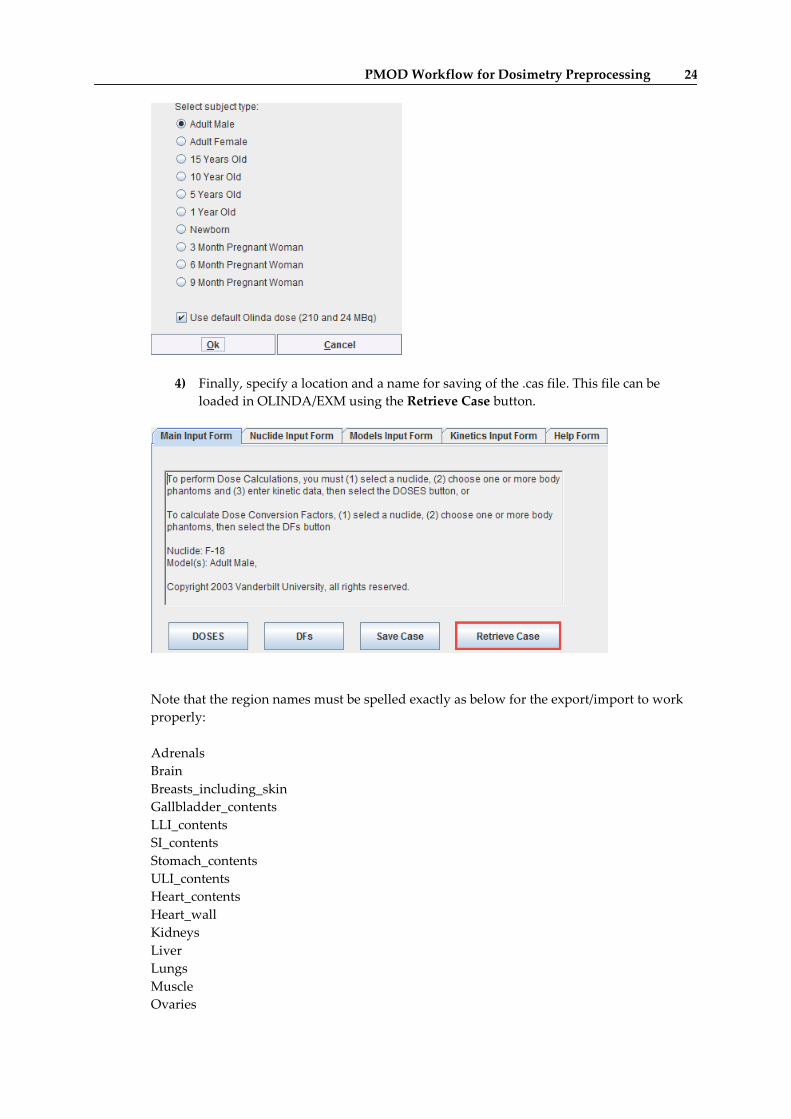
PMOD Workflow for Dosimetry Preprocessing 24
4) Finally, specify a location and a name for saving of the .cas file. This file can be
loaded in OLINDA/EXM using the Retrieve Case button.
Note that the region names must be spelled exactly as below for the export/import to work
properly:
Adrenals
Brain
Breasts_including_skin
Gallbladder_contents
LLI_contents
SI_contents
Stomach_contents
ULI_contents
Heart_contents
Heart_wall
Kidneys
Liver
Lungs
Muscle
Ovaries

PMOD Workflow for Dosimetry Preprocessing 25
Pancreas
Red_marrow
Cortical_bone
Trabecular_bone
Spleen
Testes
Thymus
Thyroid
Urinary_bladder_contents
Uterus
Fetus
Placenta
Use of the Dosimetry Organs list in VOI Properties, as described earlier in this manual, ensures
that the correct format is followed.
The difference between the injected activity and the activity accumulated in all organs is
treated as the Remainder.
Residence times can be compared between PMOD and OLINDA using the View Parameters
tool:

PMOD Workflow for Dosimetry Preprocessing 26

PMOD Workflow for Dosimetry Preprocessing 27
1) ICRU (2002) Absorbed dose specification in nuclear medicine – report no 67.
International Commission on Radiation Units and Measurements. Nuclear
Technology Publishing, Ashford
2) Nuclear Medicine Radiation Dosimetry, Advanced Theoretical Principles.
McParland BJ, ed. Springer, 2010.
3) Stabin MG and JA Siegel: Physical models and dose factors for use in internal dose
assessment. Health Physics 82003, 5(3):294-310.
4) Stabin MG, Sparks RB, Crowe E: OLINDA/EXM: the second-generation personal
computer software for internal dose assessment in nuclear medicine. J Nucl Med
2005, 46(6):1023-1027.
5) Andersson M., Johansson L., Minarik D., Mattsson S., Leide-Svegborn S. An upgrade
of the internal dosimetry computer program IDAC. In: Adliene Ny D, editor.
Medical Physics in the Baltic States 10. 2012. p. 120-123.
6) International Commission on Radiological Protection. 1990 Recommendations of the
International Commission on Radiological Protection. ICRP Publication 60,
Pergamon Press, New York, 1991.
7) ICRP, 2007. The 2007 Recommendations of the International Commission on
Radiological Protection. ICRP Publication 103. Ann. ICRP 37 (2-4).
8) ICRP, 2002. Basic Anatomical and Physiological Data for Use in Radiological
Protection Reference Values. ICRP Publication 89. Ann. ICRP 32 (3-4).
9) Stabin MG: Fundamentals of Nuclear Medicine Dosimetry. Springer; 2008.
References

PMOD Workflow for Dosimetry Preprocessing 28
Copyright © 1996-2016 PMOD Technologies LLC.
All rights reserved.
The PMOD software contains proprietary information of PMOD Technologies LLC; it is
provided under a license agreement containing restrictions on use and disclosure and is also
protected by copyright law. Reverse engineering of the software is prohibited.
Due to continued product development the program may change and no longer exactly
correspond to this document. The information and intellectual property contained herein is
confidential between PMOD Technologies LLC and the client and remains the exclusive
property of PMOD Technologies LLC. If you find any problems in the document, please
report them to us in writing. PMOD Technologies LLC does not warrant that this document
is error-free.
No part of this publication may be reproduced, stored in a retrieval system, or transmitted in
any form or by any means, electronic, mechanical, photocopying, recording or otherwise
without the prior written permission of PMOD Technologies LLC.
PMOD Technologies LLC
Sumatrastrasse 25
8006 Zürich
Switzerland
+41 (44) 350 46 00
http://www.pmod.com
PMOD Copyright Notice

29 PMOD Workflow for Dosimetry Preprocessing User's Guide
C
Conventions • 4
D
Decay Correction • 7
Delay by VOI location • 17
Dosimetry Organ List • 12
E
Edit Data • 18
Edit Patient • 18
Effective Dose • 2, 3
I
ICRP • 3, 27
IDAC • 3
Integration • 20
International Commission on Radiation Units
and Measurements • 2
Introduction • 2
M
Merge Frames Tool • 5
Model Input Parameters • 20
Model Output Parameters • 21
N
Normalized Cumulated Activity • 16
O
OLINDA • 3, 10, 12, 14, 16, 20, 23, 24, 27
OLINDA Case File Export • 23
Operational Equations • 19
P
PMOD Copyright Notice • 28
Propagate • 12
R
References • 27
residence time • 2
S
SUV PARAMETERS • 9, 18
T
Time-Activity Curve Transfer • 17
Timing Vector • 8
V
VOI Properties • 10
Index