poblano v1.0: a matlab toolbox for gradient-based optimizationacare/sand2010-1422.pdf · sandia...

SANDIA REPORTSAND2010-1422Unlimited ReleasePrinted March 2010

Poblano v1.0: A Matlab Toolbox forGradient-Based Optimization

Daniel M. Dunlavy, Tamara G. Kolda, and Evrim Acar

Prepared bySandia National LaboratoriesAlbuquerque, New Mexico 87185 and Livermore, California 94550

Sandia is a multiprogram laboratory operated by Sandia Corporation,a Lockheed Martin Company, for the United States Department of Energy’sNational Nuclear Security Administration under Contract DE-AC04-94-AL85000.

Approved for public release; further dissemination unlimited.

Issued by Sandia National Laboratories, operated for the United States Department of Energyby Sandia Corporation.

NOTICE: This report was prepared as an account of work sponsored by an agency of the UnitedStates Government. Neither the United States Government, nor any agency thereof, nor anyof their employees, nor any of their contractors, subcontractors, or their employees, make anywarranty, express or implied, or assume any legal liability or responsibility for the accuracy,completeness, or usefulness of any information, apparatus, product, or process disclosed, or rep-resent that its use would not infringe privately owned rights. Reference herein to any specificcommercial product, process, or service by trade name, trademark, manufacturer, or otherwise,does not necessarily constitute or imply its endorsement, recommendation, or favoring by theUnited States Government, any agency thereof, or any of their contractors or subcontractors.The views and opinions expressed herein do not necessarily state or reflect those of the UnitedStates Government, any agency thereof, or any of their contractors.

Printed in the United States of America. This report has been reproduced directly from the bestavailable copy.

Available to DOE and DOE contractors fromU.S. Department of EnergyOffice of Scientific and Technical InformationP.O. Box 62Oak Ridge, TN 37831

Telephone: (865) 576-8401Facsimile: (865) 576-5728E-Mail: [email protected] ordering: http://www.osti.gov/bridge

Available to the public fromU.S. Department of CommerceNational Technical Information Service5285 Port Royal RdSpringfield, VA 22161

Telephone: (800) 553-6847Facsimile: (703) 605-6900E-Mail: [email protected] ordering: http://www.ntis.gov/help/ordermethods.asp?loc=7-4-0#online

DE

PA

RT

MENT OF EN

ER

GY

• • UN

IT

ED

STATES OFA

M

ER

IC

A

2

SAND2010-1422Unlimited Release

Printed March 2010

Poblano v1.0: A Matlab Toolbox for Gradient-Based

Optimization

Daniel M. DunlavyComputer Science & Informatics Department

Sandia National Laboratories, Albuquerque, NM 87123-1318Email: [email protected]

Tamara G. Kolda and Evrim AcarInformation and Decision Sciences Department

Sandia National LaboratoriesLivermore, CA 94551-9159

Email: [email protected], [email protected]

Abstract

We present Poblano v1.0, a Matlab toolbox for solving gradient-based unconstrained optimizationproblems. Poblano implements three optimization methods (nonlinear conjugate gradients, limited-memory BFGS, and truncated Newton) that require only first order derivative information. In thispaper, we describe the Poblano methods, provide numerous examples on how to use Poblano, and presentresults of Poblano used in solving problems from a standard test collection of unconstrained optimizationproblems.

3

http://www.cs.sandia.gov/~dmdunla/

http://csmr.ca.sandia.gov/~tgkolda

http://csmr.ca.sandia.gov/~eacart

Acknowledgments

The development of Poblano was supported by Sandia’s Laboratory Directed Research & Development(LDRD) program. We thank Dianne O’Leary for providing the Matlab translation of the More-Thuente linesearch from MINPACK; MINPACK was developed by the University of Chicago, as Operator of ArgonneNational Laboratory.

4

Contents

1 Toolbox Overview . . . . . . . . . . . . . . . . . . . . . . . . . . . . . . . . . . . . . . . . . . . . . . . . . . . . . . . . . . . . . . . . . . . . . . . . . . . . . . . . 71.1 Introduction . . . . . . . . . . . . . . . . . . . . . . . . . . . . . . . . . . . . . . . . . . . . . . . . . . . . . . . . . . . . . . . . . . . 71.2 Creating an Objective Function . . . . . . . . . . . . . . . . . . . . . . . . . . . . . . . . . . . . . . . . . . . . . . . . . . . 71.3 Calling a Poblano Optimizer . . . . . . . . . . . . . . . . . . . . . . . . . . . . . . . . . . . . . . . . . . . . . . . . . . . . . . 81.4 Optimization Input Parameters . . . . . . . . . . . . . . . . . . . . . . . . . . . . . . . . . . . . . . . . . . . . . . . . . . . 91.5 Optimization Output Parameters . . . . . . . . . . . . . . . . . . . . . . . . . . . . . . . . . . . . . . . . . . . . . . . . . . 111.6 A More Complex Example Using Matrix Decomposition . . . . . . . . . . . . . . . . . . . . . . . . . . . . . . . 13

2 Optimization Methods . . . . . . . . . . . . . . . . . . . . . . . . . . . . . . . . . . . . . . . . . . . . . . . . . . . . . . . . . . . . . . . . . . . . . . . . . . . 172.1 Nonlinear Conjugate Gradient . . . . . . . . . . . . . . . . . . . . . . . . . . . . . . . . . . . . . . . . . . . . . . . . . . . . 172.2 Limited-memory BFGS . . . . . . . . . . . . . . . . . . . . . . . . . . . . . . . . . . . . . . . . . . . . . . . . . . . . . . . . . . 182.3 Truncated Newton . . . . . . . . . . . . . . . . . . . . . . . . . . . . . . . . . . . . . . . . . . . . . . . . . . . . . . . . . . . . . . 18

3 Checking Gradient Calculations . . . . . . . . . . . . . . . . . . . . . . . . . . . . . . . . . . . . . . . . . . . . . . . . . . . . . . . . . . . . . . . . . . 213.1 Difference Formulas . . . . . . . . . . . . . . . . . . . . . . . . . . . . . . . . . . . . . . . . . . . . . . . . . . . . . . . . . . . . . 213.2 Gradient Check Input Parameters . . . . . . . . . . . . . . . . . . . . . . . . . . . . . . . . . . . . . . . . . . . . . . . . . 213.3 Gradient Check Output Parameters . . . . . . . . . . . . . . . . . . . . . . . . . . . . . . . . . . . . . . . . . . . . . . . . 223.4 Examples . . . . . . . . . . . . . . . . . . . . . . . . . . . . . . . . . . . . . . . . . . . . . . . . . . . . . . . . . . . . . . . . . . . . . 22

4 Numerical Experiments . . . . . . . . . . . . . . . . . . . . . . . . . . . . . . . . . . . . . . . . . . . . . . . . . . . . . . . . . . . . . . . . . . . . . . . . . . 254.1 Description of Test Problems . . . . . . . . . . . . . . . . . . . . . . . . . . . . . . . . . . . . . . . . . . . . . . . . . . . . . 254.2 Results . . . . . . . . . . . . . . . . . . . . . . . . . . . . . . . . . . . . . . . . . . . . . . . . . . . . . . . . . . . . . . . . . . . . . . . 25

5 Conclusions . . . . . . . . . . . . . . . . . . . . . . . . . . . . . . . . . . . . . . . . . . . . . . . . . . . . . . . . . . . . . . . . . . . . . . . . . . . . . . . . . . . . . . 33References . . . . . . . . . . . . . . . . . . . . . . . . . . . . . . . . . . . . . . . . . . . . . . . . . . . . . . . . . . . . . . . . . . . . . . . . . . . . . . . . . . . . . . . . . . . 33

5

Tables

1 Input parameters for controlling amount of information displayed. . . . . . . . . . . . . . . . . . . . . . . . 102 Input parameters for controlling termination. . . . . . . . . . . . . . . . . . . . . . . . . . . . . . . . . . . . . . . . . 103 Optimization method input parameters for controlling what information is saved for each

iteration. . . . . . . . . . . . . . . . . . . . . . . . . . . . . . . . . . . . . . . . . . . . . . . . . . . . . . . . . . . . . . . . . . . . . . . 104 Optimization method input parameters for controlling line search methods. . . . . . . . . . . . . . . . 105 Output parameters returned by Poblano optimization methods. The Trace parameters are

optional, depending on whether or not tracing has been enabled . . . . . . . . . . . . . . . . . . . . . . . . 116 Conjugate direction updates available in Poblano. . . . . . . . . . . . . . . . . . . . . . . . . . . . . . . . . . . . . 177 Method-specific parameters for Poblano’s ncg optimization method. . . . . . . . . . . . . . . . . . . . . . 208 Method-specific parameters for Poblano’s lbfgs optimization method. . . . . . . . . . . . . . . . . . . . 209 Method-specific parameters for Poblano’s tn optimization method. . . . . . . . . . . . . . . . . . . . . . . 2010 Difference formulas available in Poblano for checking user-defined gradients. . . . . . . . . . . . . . . . 2111 Input parameters for Poblano’s gradientcheck function. . . . . . . . . . . . . . . . . . . . . . . . . . . . . . . 2112 Output parameters generated by Poblano’s gradientcheck function. . . . . . . . . . . . . . . . . . . . . 2213 Results of ncg using PR updates on the More, Garbow, Hillstrom test collection. Errors

greater than 10−8 are highlighted in bold, indicating that a solution was not found within thespecified tolerance. . . . . . . . . . . . . . . . . . . . . . . . . . . . . . . . . . . . . . . . . . . . . . . . . . . . . . . . . . . . . . . 27

14 Parameter changes that lead to solutions using ncg with PR updates on the More, Garbow,Hillstrom test collection. . . . . . . . . . . . . . . . . . . . . . . . . . . . . . . . . . . . . . . . . . . . . . . . . . . . . . . . . . 27

15 Results of ncg using HS updates on the More, Garbow, Hillstrom test collection. Errorsgreater than 10−8 are highlighted in bold, indicating that a solution was not found within thespecified tolerance. . . . . . . . . . . . . . . . . . . . . . . . . . . . . . . . . . . . . . . . . . . . . . . . . . . . . . . . . . . . . . . 28

16 Parameter changes that lead to solutions using ncg with HS updates on the More, Garbow,Hillstrom test collection. . . . . . . . . . . . . . . . . . . . . . . . . . . . . . . . . . . . . . . . . . . . . . . . . . . . . . . . . . 28

17 Results of ncg using FR updates on the More, Garbow, Hillstrom test collection. Errorsgreater than 10−8 are highlighted in bold, indicating that a solution was not found within thespecified tolerance. . . . . . . . . . . . . . . . . . . . . . . . . . . . . . . . . . . . . . . . . . . . . . . . . . . . . . . . . . . . . . . 29

18 Parameter changes that lead to solutions using ncg with FR updates on the More, Garbow,Hillstrom test collection. . . . . . . . . . . . . . . . . . . . . . . . . . . . . . . . . . . . . . . . . . . . . . . . . . . . . . . . . . 29

19 Results of lbfgs on the More, Garbow, Hillstrom test collection. Errors greater than 10−8

are highlighted in bold, indicating that a solution was not found within the specified tolerance. 3020 Parameter changes that lead to solutions using lbfgs on the More, Garbow, Hillstrom test

collection. . . . . . . . . . . . . . . . . . . . . . . . . . . . . . . . . . . . . . . . . . . . . . . . . . . . . . . . . . . . . . . . . . . . . . 3021 Results of tn on the More, Garbow, Hillstrom test collection. Errors greater than 10−8 are

highlighted in bold, indicating that a solution was not found within the specified tolerance. . . 3122 Parameter changes that lead to solutions using tn on the More, Garbow, Hillstrom test collection. 31

6

1 Toolbox Overview

Poblano is a toolbox of large-scale algorithms for nonlinear optimization. The algorithms in Poblano requireonly first-order derivative information (e.g., gradients for scalar-valued objective functions).

1.1 Introduction

Poblano optimizers find local minimizers of scalar-valued objective functions taking vector inputs. Specifi-cally, the problems solved by Poblano optimizers are of the following form:

minx∈RN

f(x), where f : RN → R. (1)

The gradient of the objective function, ∇f(x), is required for all Poblano optimizers. The optimizers convergeto a stationary point, x∗, where

∇f(x∗) ≈ 0.

The More-Thuente cubic interpolation line search (cvsrch) [8], satisfying the strong Wolfe conditions is usedto guarantee global convergence of the Poblano optimizers.

The following methods for solving (1) are available in Poblano; see §2 for detailed descriptions.

• Nonlinear conjugate gradient (ncg) [9]

– Uses Fletcher-Reeves, Polak-Ribiere, and Hestenes-Stiefel conjugate direction updates

– Includes restart strategies based on number of iterations or orthogonality of gradients acrossiterations

– Can do steepest descent method as a special case

• Limited-memory BFGS (lbfgs) [9]

– Uses a two-loop recursion for approximate Hessian-gradient products

• Truncated Newton (tn) [1]

– Uses finite differencing for approximate Hessian-vector products

1.2 Creating an Objective Function

Functions are passed to Poblano using Matlab function handles. The Matlab function should take a vectoras input (x ∈ RN ) and return a scalar function value (f ∈ R) as its first return value and a vector gradient(g ∈ RN ) as its second return value. Optimizing

f(x) =N∑

i=1

sin(xi).

requires the following Matlab function (which is the same for any value of N):

function [f,g] = example0(x)f = sum(sin(x));g = cos(x);

7

In the examples that follow, we use a more general function:

f(x) =N∑

i=1

sin(axi) (2)

where a is a user-defined parameter. The following example1 function (distributed with Poblano) evaluatesthe function and gradient of (2). The input parameter a is optional and defaults to a = 1. In the sectionsbelow, we show how to specify a when the function handle is passed to the optimization method.

function [f,g] = example1(x,a)if nargin < 2

a = 1;endf = sum(sin(a*x));g = a*cos(a*x);

1.3 Calling a Poblano Optimizer

Poblano methods have two required inputs as well as optional parameters discussed in the next subsection.The required arguments are 1) a function handle for the objective and gradient calculations, and 2) an initialguess of the solution (x0 ∈ RN ). For example, the call below optimizes (2) with a = 1 and N = 1; the initialguess is x0 = π/4:

>> out = ncg(@example1, pi/4);

Iter FuncEvals F(X) ||G(X)||/N------ --------- ---------------- ----------------

0 1 0.70710678 0.707106781 6 -0.99999998 0.000174072 7 -1.00000000 0.00000000

At each iteration, Poblano prints the iteration number (Iter), the total number of function evaluations(FuncEvals), the function value at the current iterate (F(X)), and the norm of the gradient at the currentiterate scaled by the problem size (||G(X)||/N). The final iterate is passed back as out.X; see §1.5 for details.

Parameterized functions can be optimized using Poblano as well by using more advanced Matlab functionhandles. We once again consider (2), but this time with N = 2, a = 3, and x0 = [π/3 π/4]T . The call belowspecifies that a = 3 by passing that as the second argument to example1. The choice of N = 2 is implicitlyspecified since x0 is in R2.

>> out = ncg(@(x) example1(x,3), [pi/3 pi/4]’)


0 1 0.70710678 1.837117311 6 -1.50761836 1.379723682 10 -1.83422986 0.827206473 13 -1.99999926 0.001828124 15 -2.00000000 0.00000001

8

1.4 Optimization Input Parameters

In this section, we discuss the input parameters that are common to all the Poblano methods and giveexamples of their use. Typing help poblano params lists these parameters. Method-specific parameters arediscussed in §2.

Table 1 lists the parameter controlling how much information displayed. For example, we can limit thedisplay to just the final iteration as follows:

>> out = ncg(@(x) example1(x,3), [pi/3 pi/4]’, ’Display’, ’final’);


4 15 -2.00000000 0.00000001

Table 2 lists the parameters controlling the stopping criteria of the optimization methods. The relativechange in the function value is defined as

|f − fold|d

where d =

{fold if fold ≥ εmach

1 if fold < εmach

with f representing the function value at the current iterate F(X), fold the function value at the previousiterate, and εmach machine epsilon (eps in Matlab). We can get a more accurate solution by tightening thetolerances, as the following example shows:

>> out = lbfgs(@(x) example1(x,2), ones(4,1), ’Display’, ’final’);


2 11 -4.00000000 0.00000001

>> out = lbfgs(@(x) example1(x,2), ones(4,1), ...’Display’, ’final’, ’StopTol’, 1e-10, ’RelFuncTol’, 0);


3 13 -4.00000000 0.00000000

Table 3 lists the parameters controlling the information that is saved for each iteration; see §1.5 for furtherdetails.

Table 4 lists the parameters controlling the behavior of the More-Thuente line search method [8]. Type helppoblano linesearch and help cvsrch for more details.

An alternative to passing a long list of parameter-value pairs is to specify the parameters in a structure. Theeasiest way to do this is to extract the default parameters (by passing a single string argument of ’defaults’as input to the Poblano optimizer to be used) and modify them, as shown in the example below.

>> params = ncg(’defaults’);>> params.Display = ’final’;>> out = ncg(@(x) example1(x,3), [pi/3 pi/4]’, params);


4 15 -2.00000000 0.00000001

9

Parameter Description Type DefaultDisplay Controls amount of printed output string ’iter’

’iter’: Display information every iteration’final’: Display information only after final iteration’off’: Display no information

Table 1: Input parameters for controlling amount of information displayed.

Parameter Description Type DefaultMaxIters Maximum number of iterations int 100MaxFuncEvals Maximum number of function evaluations int 100StopTol Gradient norm stopping tolerance, i.e., the method stops when

||G(X)||/N < StopToldouble 10−5

RelFuncTol Tolerance on relative function value change double 10−6

Table 2: Input parameters for controlling termination.

Parameter Description Type DefaultTraceX Save iterates (X) boolean falseTraceFunc Save function values (F(X)) boolean falseTraceRelFunc Save relative change in function value boolean falseTraceGrad Save the gradients (G(X)) boolean falseTraceGradNorm Save the norm of the gradients boolean falseTraceFuncEvals Save the number of function evaluations boolean false

Table 3: Optimization method input parameters for controlling what information is saved for each iteration.

Parameter Description Type DefaultLineSearch xtol Stopping tolerance for minimum change in X double 10−15

LineSearch ftol Stopping tolerance for sufficient decrease condition double 10−4

LineSearch gtol Stopping tolerance for directional derivative condition double 10−2

LineSearch stpmin Minimum step size allowed double 10−15

LineSearch stpmax Maximum step size allowed double 1015

LineSearch maxfev Maximum number of iterations allowed int 20LineSearch initialstep Initial step to be taken in the line search double 1

Table 4: Optimization method input parameters for controlling line search methods.

10

1.5 Optimization Output Parameters

The methods in Poblano outputs a structure containing the final iteration, function value, etc. The fieldsare described in Table 5. The Trace fields are optional, depending on the input parameters.

Parameter Description TypeX Final iterate vector, doubleF Function value at X doubleG Gradient at X vector, doubleParams Input parameters used for the minimization method (as parsed

Matlab inputParser object)struct

FuncEvals Number of function evaluations performed intIters Number of iterations performed (see individual optimization

routines for details on what each iteration consists of)int

ExitFlag Termination flag, with one of the following values int0 : scaled gradient norm < StopTol input parameter)1 : maximum number of iterations exceeded2 : maximum number of function values exceeded3 : relative change in function value < RelFuncTol input

parameter4 : NaNs found in F, G, or ||G||

TraceX History of iterates matrix, doubleTraceFunc History of function values vector, doubleTraceRelFunc History of relative change in function value vector, doubleTraceGrad History of gradients matrix, doubleTraceGradNorm History of norm of the gradients vector, doubleTraceFuncEvals History of the number of function evaluations vector, int

Table 5: Output parameters returned by Poblano optimization methods. The Trace parameters are optional,depending on whether or not tracing has been enabled

An example is:

>> out = ncg(@(x) example1(x,3), pi/4, ’Display’, ’final’)


2 16 -1.00000000 0.00000147

out =Params: [1x1 inputParser]

ExitFlag: 0X: 70.6858F: -1.0000G: -1.4734e-06

FuncEvals: 16Iters: 2

The exit flag (out.ExitFlag) is extremely important. A value other than zero indicates a failure to convergeto the specified tolerance. In the following example, the method uses up all its function evaluations:

11

>> out = lbfgs(@(x) example1(x,2), ones(4,1), ’Display’, ’final’, ’MaxFuncEvals’, 5)


1 9 -3.99999981 0.00030988

out =

Params: [1x1 inputParser]ExitFlag: 2

X: [4x1 double]F: -4.0000G: [4x1 double]


The number of function evaluations is only checked at the end of each iteration, so it is possible to exceedthe allowed number by up to the value specified by the input parameter LineSearch maxfev (see Table 4).

If tracing is turned on (see Table 3), then additional outputs will be returned. Here is an example:

>> out = ncg(@(x) example1(x,3), [1 2 3]’,’TraceX’,true,’TraceFunc’,true, ...’TraceRelFunc’,true,’TraceGrad’,true,’TraceGradNorm’,true,’TraceFuncEvals’,true)


0 1 0.27382300 1.652927851 5 -2.65134210 0.795229462 11 -2.93709563 0.351969063 14 -2.99999975 0.000701544 16 -3.00000000 0.00000000


ExitFlag: 0X: [3x1 double]F: -3G: [3x1 double]

FuncEvals: 16Iters: 4TraceX: [3x5 double]

TraceFunc: [0.2738 -2.6513 -2.9371 -3.0000 -3]TraceRelFunc: [10.6827 0.1078 0.0214 8.2026e-08]

TraceGrad: [3x5 double]TraceGradNorm: [4.9588 2.3857 1.0559 0.0021 2.5726e-09]TraceFuncEvals: [1 4 6 3 2]

>> X = out.X % Final function value

X =3.6652-0.52365.7596

12

>> G = out.G % Final gradient

G =1.0e-08 *0.0072-0.2052-0.1550

>> TraceX = out.TraceX % All iterates (columnwise)

TraceX =1.0000 3.7424 3.7441 3.6652 3.66522.0000 -0.6598 -0.6106 -0.5238 -0.52363.0000 5.5239 5.7756 5.7594 5.7596

>> TraceGrad = out.TraceGrad % All gradients (columnwise)

TraceGrad =-2.9700 0.6886 0.7031 0.0001 0.00002.8805 -1.1918 -0.7745 -0.0017 -0.0000-2.7334 -1.9486 0.1437 -0.0013 -0.0000

One of the outputs returned by the Poblano optimization methods is the inputParser object of the inputparameters used in that run. That object contains a field called Results, which can be passed as the inputparameters to another run. For example, this is helpful when running comparisons of methods where onlyone parameter is changed. Shown below is such an example, where default parameters are used in one run,and the same parameters with just a single change are used in another run.

>> out = ncg(@(x) example1(x,3), pi./[4 5 6]’);


0 1 2.65816330 0.771680961 7 -0.63998759 0.788695702 11 -0.79991790 0.606938193 14 -0.99926100 0.038438274 16 -0.99999997 0.000237395 18 -1.00000000 0.00000000

>> params = out.Params.Results;>> params.Display = ’final’;>> ncg(@(x) example1(x,3), pi./[4 5 6]’, params);


5 18 -1.00000000 0.00000000

1.6 A More Complex Example Using Matrix Decomposition

The following example is a more complicated function involving matrix variables. Given an m × n matrixA, the goal is to find a rank-k approximation of the form UV T . The variable x is just all the entries of U

13

and V , i.e., x = [U(:); V(:)]. Thus, the function we wish to optimize is

f(x) =12‖A− UV T‖2F (3)

where A and k have been specified. The gradient of f is

∇Uf = −(A− UV T)V

∇V f = −(A− UV T)TU.

Listed below are the contents of the example2.m file distributed with the Poblano code. The input Datacontains A and the desired rank, k. This example illustrates how x is converted to U and V for the functionand gradient computations.

function [f,g] = example2(x,Data)

% Data setup[m,n] = size(Data.A);k = Data.rank;U = reshape(x(1:m*k), m, k);V = reshape(x(m*k+1:m*k+n*k), n, k);

% Function value (residual)AmUVt = Data.A - U * V’;f = 0.5 * norm(AmUVt, ’fro’)^2;

% First derivatives computed in matrix formg = zeros((m+n)*k,1);g(1:m*k) = -reshape(AmUVt * V, m*k, 1);g(m*k+1:end) = -reshape(AmUVt’ * U, n*k, 1);

The function example2 init.m (included with Poblano) generates a test problem and starting point.

>> randn(’state’,0);>> m = 4; n = 3; k = 2;>> [x0,Data] = example2_init(m,n,k)

x0 =-0.588316543014189

2.1831858181971-0.1363958830865960.113931313520811.06676821135919

0.0592814605236053-0.095648405483669-0.8323494636500220.29441081639264-1.33618185793780.7143245518189521.62356206444627

-0.6917757017022870.857996672828263

14

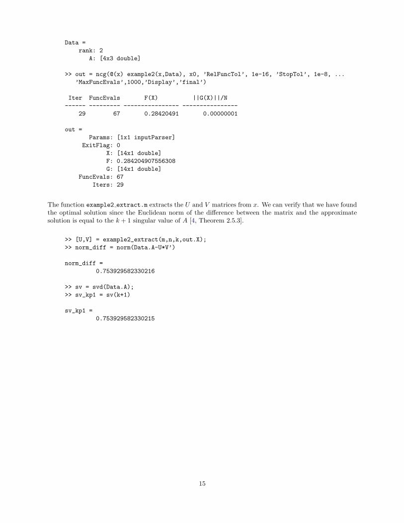
Data =rank: 2

A: [4x3 double]

>> out = ncg(@(x) example2(x,Data), x0, ’RelFuncTol’, 1e-16, ’StopTol’, 1e-8, ...’MaxFuncEvals’,1000,’Display’,’final’)


29 67 0.28420491 0.00000001


ExitFlag: 0X: [14x1 double]F: 0.284204907556308G: [14x1 double]


The function example2 extract.m extracts the U and V matrices from x. We can verify that we have foundthe optimal solution since the Euclidean norm of the difference between the matrix and the approximatesolution is equal to the k + 1 singular value of A [4, Theorem 2.5.3].

>> [U,V] = example2_extract(m,n,k,out.X);>> norm_diff = norm(Data.A-U*V’)

norm_diff =0.753929582330216

>> sv = svd(Data.A);>> sv_kp1 = sv(k+1)

sv_kp1 =0.753929582330215

15

This page intentionally left blank.

16

2 Optimization Methods

2.1 Nonlinear Conjugate Gradient

Nonlinear conjugate gradient (NCG) methods [9] are used to solve unconstrained nonlinear optimizationproblems. They are extensions of the conjugate gradient iterative method for solving linear systems adaptedto solve unconstrained nonlinear optimization problems. The Poblano function for the nonlinear conjugategradient methods is called ncg. The general steps of the NCG method are given below in pseudo-code:

1. Input: x0, a starting point2. Evaluate f0 = f(x0), g0 = ∇f(x0)3. Set p0 = −g0, i = 04. while ‖gi‖ > 05. Compute a step length αi and set xi+1 = xi + αipi

6. Set gi = ∇f(xi+1)7. Compute βi+1

8. Set pi+1 = −gi+1 + βi+1pi

9. Set i = i+ 110. end while11. Output: xi ≈ x∗

In cases where the update coefficient is negative, i.e., βi+1 < 0, it is set to 0 to avoid directions that are notdescent directions [9].

The choice of βi+1 in Step 7 leads to different NCG methods. The update methods for βi+1 are listed inTable 6. The special case of βi+1 = 0 leads to the steepest descent method [9]; see Table 7.

Update Type Update Formula

Fletcher-Reeves [3] βi+1 =gT

i+1−gi+1

gTi gi

Polak-Ribiere [12] βi+1 =gT

i+1(gi+1−gi)gT

i gi

Hestenes-Stiefel [5] βi+1 =gT

i+1(gi+1−gi)pT

i (gi+1−gi)

Table 6: Conjugate direction updates available in Poblano.

The NCG iterations are restarted every k iterations, where k is specified via the RestartIters parameter.The default is 20.

Another restart modification that was suggested by Nocedal and Wright [9] is taking a step in the directionof steepest descent when two consecutive gradients are far from orthogonal. Specifically, a steepest descentstep is taken whenever

|gTi+1gi|‖gi+1‖

≥ ν

where ν is specified via the RestartNWTol parameter. This modification is off by default, but can be usedby setting RestartNW to true.

The input parameters specific to the ncg method are presented in Table 7.

17

2.2 Limited-memory BFGS

Limited-memory quasi-Newton methods [9] are a class of methods that compute and/or maintain simple,compact approximations of the Hessian matrices of second derivatives, which are used determining searchdirections. Poblano includes the limited-memory BFGS (L-BFGS) method, a variant of these methods whoseHessian approximations are based on the BFGS method (see [2] for more details). The Poblano function forthe L-BFGS method is called lbfgs. The general steps of L-BFGS methods are given below in pseudo-code[9]:

1. Input: x0, a starting point; M > 0, an integer2. Evaluate f0 = f(x0), g0 = ∇f(x0)3. Set p0 = −g0, γ0 = 1, i = 04. while ‖gi‖ > 05. Choose an initial Hessian approximation: H0

i = γiI6. Compute a step direction pi = −r using TwoLoopRecursion method7. Compute a step length αi and set xi+1 = xi + αipi

8. Set gi = ∇f(xi+1)9. if i > M10. Discard vectors {si−m, yi−m} from storage11. end if12. Set and store si = xi+1 − xi and yi = gi+1 − gi

13. Set i = i+ 114. end while15. Output: xi ≈ x∗

In Step 6 in the above method, the computation of the step direction is performed using the following method(assume we are at iteration i) [9]:

TwoLoopRecursion1. q = gi

2. for k = i− 1, i− 2, . . . , i−m3. ak = (sT

k q)/(yTk sk)

4. q = q − akyk

5. end for6. r = H0

i q7. for k = i−m, i−m+ 1, . . . , i− 18. b = (yT

k r)/(yTk sk)

9. r = r + (ak − b)sk

10. end for11. Output: r = Higi

The input parameters specific to the lbfgs method are presented in Table 8.

2.3 Truncated Newton

Truncated Newton (TN) methods for minimization are Newton methods in which the Newton direction isonly approximated at each iteration (thus reducing computation). Furthermore, the Poblano implementationof the truncated Newton method does not require an explicit Hessian matrix in the computation of theapproximate Newton direction (thus reducing storage requirements). The Poblano function for the truncated

18

Newton method is called tn. The general steps of TN methods are given below in pseudo-code [1]:

1. Input: x0, a starting point2. Evaluate f0 = f(x0), g0 = ∇f(x0)3. Set i = 04. while ‖gi‖ > 05. Compute the conjugate gradient stopping tolerance, ηi

6. Compute pi by solving ∇2f(xi)p = −gi using a linear conjugate gradient (CG) method7. Compute a step length αi and set xi+1 = xi + αipi

8. Set gi = ∇f(xi+1)9. Set i = i+ 110. end while11. Output: xi ≈ x∗

In Step 5, the linear conjugate gradient (CG) method stopping tolerance is allowed to change at eachiteration. The input parameter CGTolType determines how ηi is computed.

In Step 6, we note the following.

• One of Matlab’s CG methods is used to solve for pi: symmlq (designed for symmetric indefinite sys-tems) or pcg (the classical CG method for symmetric positive definite systems). The input parameterCGSolver controls the choice of CG method to use.

• The maximum number of CG iterations is specified using the input parameter CGIters.

• The CG method stops when ‖ − gi −∇2f(xi)pi‖ ≤ ηi‖gi‖ .

• In the CG method, matrix-vector products involving ∇2f(xi) times a vector v are approximated usingthe following finite difference approximation [1]:

∇2f(xi)v ≈∇f(xi + σv)−∇f(xi)

σ

The difference step, σ, is specified using the input parameter HessVecFDStep. The computation of thefinite difference approximation is performed using the hessvec fd provided with Poblano.

The input parameters specific to the tn method are presented in Table 9.

19

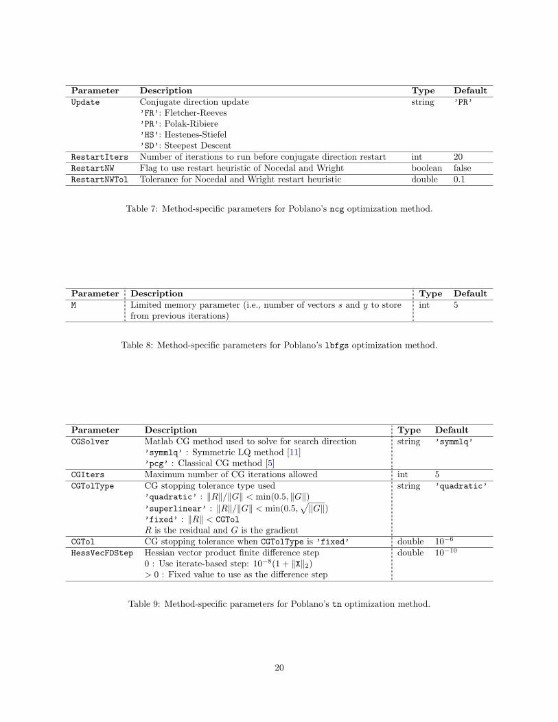
Parameter Description Type DefaultUpdate Conjugate direction update string ’PR’

’FR’: Fletcher-Reeves’PR’: Polak-Ribiere’HS’: Hestenes-Stiefel’SD’: Steepest Descent

RestartIters Number of iterations to run before conjugate direction restart int 20RestartNW Flag to use restart heuristic of Nocedal and Wright boolean falseRestartNWTol Tolerance for Nocedal and Wright restart heuristic double 0.1

Table 7: Method-specific parameters for Poblano’s ncg optimization method.

Parameter Description Type DefaultM Limited memory parameter (i.e., number of vectors s and y to store

from previous iterations)int 5

Table 8: Method-specific parameters for Poblano’s lbfgs optimization method.

Parameter Description Type DefaultCGSolver Matlab CG method used to solve for search direction string ’symmlq’

’symmlq’ : Symmetric LQ method [11]’pcg’ : Classical CG method [5]

CGIters Maximum number of CG iterations allowed int 5CGTolType CG stopping tolerance type used string ’quadratic’

’quadratic’ : ‖R‖/‖G‖ < min(0.5, ‖G‖)’superlinear’ : ‖R‖/‖G‖ < min(0.5,

√‖G‖)

’fixed’ : ‖R‖ < CGTolR is the residual and G is the gradient

CGTol CG stopping tolerance when CGTolType is ’fixed’ double 10−6

HessVecFDStep Hessian vector product finite difference step double 10−10

0 : Use iterate-based step: 10−8(1 + ‖X‖2)> 0 : Fixed value to use as the difference step

Table 9: Method-specific parameters for Poblano’s tn optimization method.

20

3 Checking Gradient Calculations

Analytic gradients can be checked using finite difference approximations. The Poblano functiongradientcheck computes the gradient approximations and compares the results to the analytic gradientusing a user-supplied objective function/gradient M-file. The user can choose one of several difference for-mulas as well as the difference step used in the computations.

3.1 Difference Formulas

The difference formulas for approximating the gradients in Poblano are listed in Table 10. For more detailson the formulas, see [9].

Formula Type Formula

Forward Differences∂f

∂xi(x) ≈ f(x+ hei)− f(x)

h

Backward Differences∂f

∂xi(x) ≈ f(x)− f(x− hei)

h

Centered Differences∂f

∂xi(x) ≈ f(x+ hei)− f(x− hei)

2h

Note: ei is a vector the same size as x with a 1 in element i and zeros elsewhere,

and h is a user-defined parameter.

Table 10: Difference formulas available in Poblano for checking user-defined gradients.

The type of finite differences to use is specified using the DifferenceType input parameter, and the valueof h is specified using the DifferenceStep input parameter. For a detailed discussion on the impact of thechoice of h on the quality of the approximation, see [10].

3.2 Gradient Check Input Parameters

The input parameters available for the gradientcheck function are presented in Table 11.

Parameter Description Type DefaultDifferenceType Difference formula to use string ’forward’

’forward’: gi = (f(x+ hei)− f(x))/h’backward’: gi = (f(x)− f(x− hei))/h’centered’: gi = (f(x+ hei)− f(x− hei))/(2h)

DifferenceStep Value of h in difference formulae double 10−8

Table 11: Input parameters for Poblano’s gradientcheck function.

21

3.3 Gradient Check Output Parameters

The fields in the output structure generated by the gradientcheck function are presented in Table 12.

Parameter Description TypeG Analytic gradient vector, doubleGFD Finite difference approximation of gradient vector, doubleMaxDiff Maximum difference between G and GFD doubleMaxDiffInd Index of maximum difference between G and GFD intNormGradientDiffs Norm of the difference between gradients: ‖G− GFD‖2 doubleGradientDiffs G - GFD vector, doubleParams Input parameters used to compute approximations struct

Table 12: Output parameters generated by Poblano’s gradientcheck function.

3.4 Examples

We use example1 (distributed with Poblano) to illustrate how to use the gradientcheck function to checkuser-supplied gradients. The user provides a function handle to the M-file containing their function andgradient computations, a point at which to check the gradients, and the type of difference formula to use.Below are examples of running the gradient check using each of the difference formulas.

>> outFD = gradientcheck(@(x) example1(x,3), pi./[4 5 6]’,’DifferenceType’,’forward’)

outFD =G: [3x1 double]

GFD: [3x1 double]MaxDiff: 6.4662e-08

MaxDiffInd: 1NormGradientDiffs: 8.4203e-08

GradientDiffs: [3x1 double]Params: [1x1 struct]

>> outBD = gradientcheck(@(x) example1(x,3), pi./[4 5 6]’,’DifferenceType’,’backward’)

outBD =G: [3x1 double]

GFD: [3x1 double]MaxDiff: -4.4409e-08



22

>> outCD = gradientcheck(@(x) example1(x,3), pi./[4 5 6]’,’DifferenceType’,’centered’)

outCD =G: [3x1 double]

GFD: [3x1 double]MaxDiff: 2.0253e-08



Note the different gradients produced using the various differencing formulas:

>> [outFD.G outFD.GFD outBD.GFD outCD.GFD]

ans =-2.121320343559642 -2.121320408221550 -2.121320319403708 -2.121320363812629-0.927050983124842 -0.927051013732694 -0.927050969323773 -0.9270509915282330.000000000000000 -0.000000044408921 0.000000044408921 0

23


24

4 Numerical Experiments

To demonstrate the performance of the Poblano methods, we present results of runs of the different methodsin this section. All experiments were performed using Matlab 7.9 on a Linux Workstation (RedHat 5.2) with2 Quad-Core Intel Xeon 3.0GHz processors and 32GB RAM.

4.1 Description of Test Problems

The test problems used in the experiments presented here are from the More, Garbow, and Hillstromcollection, which is described in detail in [7]. The Matlab code used for these problems, along with the knownoptima, is provided as part of the SolvOpt optimization software [6], available at http://www.kfunigraz.ac.at/imawww/kuntsevich/solvopt/. (SolvOpt is an implementation of Shor’s r-algorithm for non-smoothoptimization [13] with additional heuristics for computing search directions and stopping criteria, but hasbeen tested using this collection, which contains continuously differentiable problems.) There are 34 testproblems in this collection.

4.2 Results

Results in this section are for optimization runs using the default parameters, with the exception of the stop-ping criteria parameters, which were changed to allow more computation and find more accurate solutions.The parameters changed from their default values are as follows:

params.Display = ’off’params.MaxIters = 20000;params.MaxFuncEvals = 50000;params.RelFuncTol = 1e-16;params.StopTol = 1e-12;

For the results presented in this section, the function value computed by the Poblano methods is denotedby F ∗, the solution (i.e., the best known function value reported in the literature) is denoted by F ∗, and the(relative) error is |F ∗ − F ∗|/max{1, |F ∗|}.

For this test collection, we say the problem is solved if the relative error is less than 10−8. We see that thePoblano methods solve most of the problems using the default input parameters, but have difficulty with afew that require particular parameter settings. Specifically, the initial step size in the line search methodappears to be the most sensitive parameter across the methods. More investigation into the effective use ofthis parameter for other problem classes is planned for future work. Below are more details of the resultsfor the different Poblano methods.

4.2.1 Nonlinear Conjugate Gradient

The results of the tests for the ncg method using Polak-Ribiere (PR) conjugate direction updates are pre-sented in Table 13. Note that several problems (3, 6, 10, 11, 17, 20, 27 and 31) were not solved using theparameters listed above. With more testing, specifically with different values of the initial step size used inthe line search (specified using the LineSearch initialstep parameter) and the number of iterations toperform before restarting the conjugate directions using a step in the steepest direction (specified using theRestartIters parameter), solutions to all problems except #10 were found. Table 14 presents parameterchoices leading to successful runs of the ncg method using PR conjugate direction updates.

25

http://www.kfunigraz.ac.at/imawww/kuntsevich/solvopt/


The results of the tests for the ncg method using Hestenes-Stiefel (HS) conjugate direction updates arepresented in Table 15. Again, several problems (3, 6, 10, 11 and 31) were not solved using the parameterslisted above. Table 16 presents parameter choices leading to successful runs of the ncg method using HSconjugate direction updates. Note that we did not find parameters to solve problem #10 with this methodeither.

Finally, the results of the tests for the ncg method using Fletcher-Reeves (FR) conjugate direction updatesare presented in Table 17. We see that even more problems (3, 6, 10, 11, 17, 18, 20 and 31) were not solvedusing the parameters listed above. Table 18 presents parameter choices leading to successful runs of the ncgmethod using FR conjugate direction updates. Note that we did not find parameters to solve problem #10with this method either.

4.2.2 Limited-memory BFGS

The results of the tests for the lbfgs method are presented in Table 19. Compared to the ncg methods,fewer problems (6, 11, 18 and 31) were not solved using the parameters listed above with the lbfgs method.Most notably, lbfgs was able to solve problem #10, illustrating that some problems are better suited to thedifferent Poblano methods. With more testing, specifically with different values of the initial step size usedin the line search (specified using the LineSearch initialstep parameter), solutions to all problems werefound. Table 20 presents parameter choices leading to successful runs of the lbfgs method.

4.2.3 Truncated Newton

The results of the tests for the tn method are presented in Table 21. Note that several problems (10, 11, 20and 31) were not solved using this method. However, problem #6 was solved (which was not solved usingany of the other Poblano methods), again illustrating that some problems are better suited to tn than theother Poblano methods. With more testing, specifically with different values of the initial step size usedin the line search (specified using the LineSearch initialstep parameter), solutions to all problems werefound, with the exception of problem #10. Table 22 presents parameter choices leading to successful runsof the tn method.

26

# Exit Iters FuncEvals F ∗ F ∗ Error

1 3 20 90 1.3972e-18 0.0000e+00 1.3972e-18

2 3 11 71 4.8984e+01 4.8984e+01 5.8022e-16

3 3 3343 39373 6.3684e-07 0.0000e+00 6.3684e-07

4 3 14 126 1.4092e-21 0.0000e+00 1.4092e-21

5 3 12 39 1.7216e-17 0.0000e+00 1.7216e-17

6 0 1 8 2.0200e+03 1.2436e+02 1.5243e+01

7 3 53 158 5.2506e-18 0.0000e+00 5.2506e-18

8 3 28 108 8.2149e-03 8.2149e-03 1.2143e-17

9 0 5 14 1.1279e-08 1.1279e-08 2.7696e-14

10 3 262 1232 9.5458e+04 8.7946e+01 1.0844e+03

11 0 1 2 3.8500e-02 0.0000e+00 3.8500e-02

12 0 15 62 3.9189e-32 0.0000e+00 3.9189e-32

13 3 129 352 1.5737e-16 0.0000e+00 1.5737e-16

14 3 47 155 2.7220e-18 0.0000e+00 2.7220e-18

15 3 58 165 3.0751e-04 3.0751e-04 3.9615e-10

16 3 34 168 8.5822e+04 8.5822e+04 4.3537e-09

17 3 3122 7970 5.5227e-05 5.4649e-05 5.7842e-07

18 3 1181 2938 2.1947e-16 0.0000e+00 2.1947e-16

19 3 381 876 4.0138e-02 4.0138e-02 2.9355e-10

20 3 14842 30157 1.4233e-06 1.4017e-06 2.1546e-08

21 3 20 90 6.9775e-18 0.0000e+00 6.9775e-18

22 3 129 352 1.5737e-16 0.0000e+00 1.5737e-16

23 0 90 415 2.2500e-05 2.2500e-05 2.4991e-11

24 3 142 520 9.3763e-06 9.3763e-06 7.4196e-15

25 3 5 27 7.4647e-25 0.0000e+00 7.4647e-25

26 3 47 144 2.7951e-05 2.7951e-05 2.1878e-13

27 3 2 8 8.2202e-03 0.0000e+00 8.2202e-03

28 3 79 160 1.4117e-17 0.0000e+00 1.4117e-17

29 3 7 16 9.1648e-19 0.0000e+00 9.1648e-19

30 3 30 75 1.0410e-17 0.0000e+00 1.0410e-17

31 3 41 97 3.0573e+00 0.0000e+00 3.0573e+00

32 0 2 5 1.0000e+01 1.0000e+01 0.0000e+00

33 3 2 5 4.6341e+00 4.6341e+00 0.0000e+00

34 3 2 5 6.1351e+00 6.1351e+00 0.0000e+00

Table 13: Results of ncg using PR updates on the More, Garbow, Hillstrom test collection. Errors greaterthan 10−8 are highlighted in bold, indicating that a solution was not found within the specified tolerance.

# Input Parameters Iters FuncEvals F ∗ Error

3 LineSearch initialstep = 1e-5 19 152 9.9821e-09 9.9821e-09

RestartIters = 40

6 LineSearch initialstep = 1e-5 19 125 1.2436e+02 3.5262e-11

RestartIters = 40


RestartIters = 40



RestartIters = 50

27 LineSearch initialstep = 0.5 11 38 1.3336e-25 1.3336e-25


Table 14: Parameter changes that lead to solutions using ncg with PR updates on the More, Garbow,Hillstrom test collection.

27


1 3 20 89 1.0497e-16 0.0000e+00 1.0497e-16

2 3 10 69 4.8984e+01 4.8984e+01 2.9011e-16

3 2 4329 50001 4.4263e-08 0.0000e+00 4.4263e-08

4 3 9 83 1.3553e-18 0.0000e+00 1.3553e-18

5 3 12 39 4.3127e-19 0.0000e+00 4.3127e-19

6 0 1 8 2.0200e+03 1.2436e+02 1.5243e+01

7 3 27 98 1.8656e-20 0.0000e+00 1.8656e-20

8 3 25 92 8.2149e-03 8.2149e-03 1.2143e-17

9 3 5 31 1.1279e-08 1.1279e-08 2.7696e-14

10 3 49 332 1.0856e+05 8.7946e+01 1.2334e+03

11 0 1 2 3.8500e-02 0.0000e+00 3.8500e-02

12 0 15 63 5.8794e-30 0.0000e+00 5.8794e-30

13 3 84 258 2.7276e-17 0.0000e+00 2.7276e-17

14 3 44 152 3.4926e-24 0.0000e+00 3.4926e-24

15 3 50 165 3.0751e-04 3.0751e-04 3.9615e-10

16 3 39 176 8.5822e+04 8.5822e+04 4.3537e-09

17 3 942 2754 5.4649e-05 5.4649e-05 4.3964e-12

18 3 748 1977 2.7077e-18 0.0000e+00 2.7077e-18

19 3 237 607 4.0138e-02 4.0138e-02 2.9356e-10

20 3 4685 9977 1.3999e-06 1.4017e-06 1.7946e-09

21 0 22 93 6.1630e-32 0.0000e+00 6.1630e-32

22 3 84 258 2.7276e-17 0.0000e+00 2.7276e-17

23 0 83 381 2.2500e-05 2.2500e-05 2.4991e-11

24 3 170 691 9.3763e-06 9.3763e-06 7.3568e-15

25 3 5 47 7.4570e-25 0.0000e+00 7.4570e-25

26 3 43 144 2.7951e-05 2.7951e-05 2.1878e-13

27 3 9 40 2.5738e-20 0.0000e+00 2.5738e-20

28 3 33 70 8.3475e-18 0.0000e+00 8.3475e-18

29 3 7 16 9.1699e-19 0.0000e+00 9.1699e-19

30 3 29 73 3.4886e-18 0.0000e+00 3.4886e-18

31 3 33 117 3.0573e+00 0.0000e+00 3.0573e+00

32 0 2 5 1.0000e+01 1.0000e+01 0.0000e+00

33 3 2 5 4.6341e+00 4.6341e+00 0.0000e+00

34 3 2 5 6.1351e+00 6.1351e+00 0.0000e+00

Table 15: Results of ncg using HS updates on the More, Garbow, Hillstrom test collection. Errors greaterthan 10−8 are highlighted in bold, indicating that a solution was not found within the specified tolerance.



RestartIters = 40



RestartIters = 40


Table 16: Parameter changes that lead to solutions using ncg with HS updates on the More, Garbow,Hillstrom test collection.

28


1 3 41 199 2.4563e-17 0.0000e+00 2.4563e-17

2 3 25 104 4.8984e+01 4.8984e+01 4.3517e-16

3 3 74 538 1.2259e-03 0.0000e+00 1.2259e-03

4 3 40 304 2.9899e-13 0.0000e+00 2.9899e-13

5 3 27 76 4.7847e-17 0.0000e+00 4.7847e-17

6 0 1 8 2.0200e+03 1.2436e+02 1.5243e+01

7 3 48 153 3.5829e-19 0.0000e+00 3.5829e-19

8 3 46 144 8.2149e-03 8.2149e-03 3.4694e-18

9 3 7 72 1.1279e-08 1.1279e-08 2.7696e-14

10 3 388 2098 3.0166e+04 8.7946e+01 3.4201e+02

11 0 1 2 3.8500e-02 0.0000e+00 3.8500e-02

12 3 19 65 2.6163e-18 0.0000e+00 2.6163e-18

13 3 308 720 1.8955e-16 0.0000e+00 1.8955e-16

14 3 53 219 3.0620e-17 0.0000e+00 3.0620e-17

15 3 83 232 3.0751e-04 3.0751e-04 3.9615e-10

16 3 42 206 8.5822e+04 8.5822e+04 4.3537e-09

17 3 522 2020 5.5389e-05 5.4649e-05 7.4046e-07

18 3 278 644 5.6432e-03 0.0000e+00 5.6432e-03

19 3 385 1003 4.0138e-02 4.0138e-02 2.9355e-10

20 3 14391 29061 2.7316e-06 1.4017e-06 1.3298e-06

21 3 41 199 1.2282e-16 0.0000e+00 1.2282e-16

22 3 308 720 1.8955e-16 0.0000e+00 1.8955e-16

23 3 192 783 2.2500e-05 2.2500e-05 2.4991e-11

24 3 1239 4256 9.3763e-06 9.3763e-06 7.3782e-15

25 0 5 29 1.7256e-31 0.0000e+00 1.7256e-31

26 3 60 187 2.7951e-05 2.7951e-05 2.1877e-13

27 3 10 34 1.0518e-16 0.0000e+00 1.0518e-16

28 3 112 226 1.7248e-16 0.0000e+00 1.7248e-16

29 3 7 16 1.9593e-18 0.0000e+00 1.9593e-18

30 3 30 74 1.1877e-17 0.0000e+00 1.1877e-17

31 3 58 166 3.0573e+00 0.0000e+00 3.0573e+00

32 0 2 5 1.0000e+01 1.0000e+01 3.5527e-16

33 3 2 5 4.6341e+00 4.6341e+00 0.0000e+00

34 3 2 5 6.1351e+00 6.1351e+00 0.0000e+00

Table 17: Results of ncg using FR updates on the More, Garbow, Hillstrom test collection. Errors greaterthan 10−8 are highlighted in bold, indicating that a solution was not found within the specified tolerance.



RestartIters = 50



RestartIters = 40


RestartIters = 40



RestartIters = 50


Table 18: Parameter changes that lead to solutions using ncg with FR updates on the More, Garbow,Hillstrom test collection.

29


1 3 43 145 1.5549e-20 0.0000e+00 1.5549e-20

2 3 14 73 4.8984e+01 4.8984e+01 4.3517e-16

3 3 206 730 5.8432e-20 0.0000e+00 5.8432e-20

4 3 14 29 7.8886e-31 0.0000e+00 7.8886e-31

5 3 20 55 1.2898e-24 0.0000e+00 1.2898e-24

6 0 1 8 2.0200e+03 1.2436e+02 1.5243e+01

7 0 40 103 8.6454e-28 0.0000e+00 8.6454e-28

8 0 27 63 8.2149e-03 8.2149e-03 1.7347e-18

9 0 4 9 1.1279e-08 1.1279e-08 2.7696e-14

10 3 705 2406 8.7946e+01 8.7946e+01 4.2594e-13

11 0 1 2 3.8500e-02 0.0000e+00 3.8500e-02

12 3 24 76 3.2973e-20 0.0000e+00 3.2973e-20

13 3 77 165 1.7747e-17 0.0000e+00 1.7747e-17

14 3 66 187 1.2955e-19 0.0000e+00 1.2955e-19

15 0 29 72 3.0751e-04 3.0751e-04 3.9615e-10

16 3 22 96 8.5822e+04 8.5822e+04 4.3537e-09

17 3 221 602 5.4649e-05 5.4649e-05 9.7483e-13

18 3 56 165 5.6556e-03 0.0000e+00 5.6556e-03

19 3 267 713 4.0138e-02 4.0138e-02 2.9355e-10

20 3 5118 10752 1.3998e-06 1.4017e-06 1.9194e-09

21 3 44 146 2.8703e-24 0.0000e+00 2.8703e-24

22 3 77 165 1.7747e-17 0.0000e+00 1.7747e-17

23 0 218 786 2.2500e-05 2.2500e-05 2.4991e-11

24 3 458 1492 9.3763e-06 9.3763e-06 7.3554e-15

25 0 4 31 1.4730e-29 0.0000e+00 1.4730e-29

26 3 41 135 2.7951e-05 2.7951e-05 2.1879e-13

27 3 15 37 9.7350e-24 0.0000e+00 9.7350e-24

28 3 67 140 1.2313e-16 0.0000e+00 1.2313e-16

29 3 7 15 2.5466e-21 0.0000e+00 2.5466e-21

30 3 25 54 1.5036e-17 0.0000e+00 1.5036e-17

31 3 27 100 3.0573e+00 0.0000e+00 3.0573e+00

32 0 2 4 1.0000e+01 1.0000e+01 7.1054e-16

33 3 2 4 4.6341e+00 4.6341e+00 0.0000e+00

34 3 2 4 6.1351e+00 6.1351e+00 0.0000e+00

Table 19: Results of lbfgs on the More, Garbow, Hillstrom test collection. Errors greater than 10−8 arehighlighted in bold, indicating that a solution was not found within the specified tolerance.




18 LineSearch initialstep = 0 220 1102 9.3766e-17 9.3766e-17

M = 1


Table 20: Parameter changes that lead to solutions using lbfgs on the More, Garbow, Hillstrom testcollection.

30


1 0 105 694 4.9427e-30 0.0000e+00 4.9427e-30

2 3 9 107 4.8984e+01 4.8984e+01 2.9011e-16

3 3 457 3607 3.1474e-09 0.0000e+00 3.1474e-09

4 0 6 36 0.0000e+00 0.0000e+00 0.0000e+00

5 0 13 96 4.4373e-31 0.0000e+00 4.4373e-31

6 3 13 133 1.2436e+02 1.2436e+02 3.5262e-11

7 0 39 245 6.9237e-46 0.0000e+00 6.9237e-46

8 0 9 80 8.2149e-03 8.2149e-03 8.6736e-18

9 0 3 28 1.1279e-08 1.1279e-08 2.7696e-14

10 2 6531 50003 1.1104e+05 8.7946e+01 1.2616e+03

11 0 1 5 3.8500e-02 0.0000e+00 3.8500e-02

12 0 9 74 1.8615e-28 0.0000e+00 1.8615e-28

13 0 25 241 2.3427e-29 0.0000e+00 2.3427e-29

14 0 36 263 1.0481e-26 0.0000e+00 1.0481e-26

15 0 449 4967 3.0751e-04 3.0751e-04 3.9615e-10

16 3 28 237 8.5822e+04 8.5822e+04 4.3537e-09

17 3 2904 30801 5.4649e-05 5.4649e-05 3.3347e-10

18 3 2622 28977 6.3011e-17 0.0000e+00 6.3011e-17

19 3 526 5671 4.0138e-02 4.0138e-02 2.9355e-10

20 2 4654 50006 6.0164e-06 1.4017e-06 4.6147e-06

21 0 96 638 3.9542e-28 0.0000e+00 3.9542e-28

22 0 25 241 2.3427e-29 0.0000e+00 2.3427e-29

23 0 17 207 2.2500e-05 2.2500e-05 2.4991e-11

24 0 63 827 9.3763e-06 9.3763e-06 7.3554e-15

25 0 3 19 2.3419e-31 0.0000e+00 2.3419e-31

26 3 18 249 2.7951e-05 2.7951e-05 2.1878e-13

27 0 6 53 2.7820e-29 0.0000e+00 2.7820e-29

28 3 82 882 1.9402e-17 0.0000e+00 1.9402e-17

29 0 4 33 9.6537e-32 0.0000e+00 9.6537e-32

30 3 16 104 3.4389e-21 0.0000e+00 3.4389e-21

31 3 13 145 3.0573e+00 0.0000e+00 3.0573e+00

32 3 4 63 1.0000e+01 1.0000e+01 5.3291e-16

33 3 4 48 4.6341e+00 4.6341e+00 1.9166e-16

34 3 3 19 6.1351e+00 6.1351e+00 0.0000e+00

Table 21: Results of tn on the More, Garbow, Hillstrom test collection. Errors greater than 10−8 arehighlighted in bold, indicating that a solution was not found within the specified tolerance.



HessVecFDStep = 1e-12

20 CGIters = 50 34 1336 1.3998e-06 1.9715e-09


Table 22: Parameter changes that lead to solutions using tn on the More, Garbow, Hillstrom test collection.

31


32

5 Conclusions

We have presented Poblano v1.0, a Matlab Toolbox for unconstrained optimization requiring only firstorder derivatives. Details of the methods available in Poblano as well as how to use the toolbox to solveunconstrained optimization problems were provided. Demonstration of the Poblano solvers on the More,Garbow and Hillstrom collection of test problems indicates good performance in general of the Poblanooptimizer methods across a wide range of problems.

33

References

[1] R. Dembo and T. Steihaug, Truncated-Newton algorithms for large-scale unconstrained optimization,Mathematical Programming, 26 (1983), pp. 190–212.

[2] J. E. Dennis, Jr. and R. B. Schnabel, Numerical Methods for Unconstrained Optimization andNonlinear Equations, SIAM, Philadelphia, PA, 1996. Corrected reprint of the 1983 original.

[3] R. Fletcher and C. Reeves, Function minimization by conjugate gradients, The Computer Journal,7 (1964), pp. 149–154.

[4] G. H. Golub and C. F. Van Loan, Matrix Computations, Johns Hopkins Univ. Press, 1996.

[5] M. R. Hestenes and E. Stiefel, Methods of conjugate gradients for solving linear systems, J. Res.Nat. Bur. Standards Sec. B., 48 (1952), pp. 409–436.

[6] A. Kuntsevich and F. Kappel, SolvOpt: The solver for local nonlinear optimization problems, tech.rep., Institute for Mathematics, Karl-Franzens University of Graz, June 1997. http://www.kfunigraz.ac.at/imawww/kuntsevich/solvopt/.

[7] J. J. More, B. S. Garbow, and K. E. Hillstrom, Testing unconstrained optimization software,ACM Trans. Math. Software, 7 (1981), pp. 17–41.

[8] J. J. More and D. J. Thuente, Line search algorithms with guaranteed sufficient decrease, ACMTransactions on Mathematical Software, 20 (1994), pp. 286–307.

[9] J. Nocedal and S. J. Wright, Numerical Optimization, Springer, 1999.

[10] M. L. Overton, Numerical Computing with IEEE Floating Point Arithmetic, Society for Industrialand Applied Mathematics, 2001.

[11] C. C. Paige and M. A. Saunders, Solution of sparse indefinite systems of linear equations, SIAMJ. Numer. Anal., Vol.12 (1975), pp. 617–629.

[12] E. Polak and G. Ribiere, Note sur la convergence de methods de directions conjugres, Revue Fran-caise Informat. Recherche Operationnelle, 16 (1969), pp. 35–43.

[13] N. Z. Shor, Minimization methods for Non-Differentiable Functions, vol. 3 of Series in ComputationalMathematics, Springer-Verlag, Berlin, 1985.

34



DISTRIBUTION:

5 MS 1318 Daniel M. Dunlavy, 14151 MS 1318 Brett Bader, 14151 MS 9159 Heidi Ammerlahn, 89625 MS 9159 Tamara G. Kolda, 8962

1 MS 0899 Technical Library, 9536 (electronic)1 MS 0123 D. Chavez, LDRD Office, 1011

35

poblano v1.0: a matlab toolbox for gradient-based optimizationacare/sand2010-1422.pdf · sandia...

Documents