Point Location

Dmitry Rusakov

Boris Kronrod

Planar Point Location

Lets S be a planar subdivision with n edges. The planar point location problem is to store S in such a way that we can answer queries of the following type:

Given a query point q, report a face f of S that contains q. If q lies on an edge or coincides with a vertex, the query algorithm, should return this information.

Algorithm requirements

• There’re situations, like interactive geographic information system, where system must respond very fast to each query. So we need fast algorithm.

• In the same time, the complexity of data structure, that algorithm is using, must be small since typical geographic information system includes a large number of regions.

Naive Approach

• Hold a list of faces, for each face hold a list of border edges of this face.

• For query point q find a face that includes q, by checking faces one by one.

• Space complexity: O(n)

• Time complexity: O(n), because each edge is checked maximum twice.

Naive Approach - Analysis

• O(n) time complexity is too big for real applications.

• Source of the problem - checking against all faces. In hope to achieve O(log n) time, we must sort faces in some way, which is impossible with complex faces.

• Solution - work with simple space subdivisions.

Refinement

• Subdivision S` is refinement of subdivision S if every face of S` lies completely in one face of S.

• Once we know the face f` of S` containing q, we know the face f of S containing q as well.

Partition into Slabs

• Partition the plane into vertical slabs, by drawing vertical lines through all vertices of the given subdivision S.

• For query point q, find a slab it belongs to and find a corresponding face in this slab.

Partition into Slabs, Example

Slab properties

• Within a slab, there’re no vertices of S.

• All edges intersecting a slab completely cross it and they don’t cross each other.

Data Structure

• Slabs sorted by x coordinate.n slabs are stored in binary tree allowing O(log n) search time.

• In each slab we sort an edges intersecting it according to above-below relationship.n edges intersecting the slab are stored in binary tree allowing O(log n) search time.

• Worst case: O(n2) storage complexity.

O(n2) storage case

n/4 slabs

Query

• Find a slab containing q. O(log n) time.

• Find an edge immediately above(below) q in found slab. O(log n) time.

• Each edge uniquely defines a face below(above) it.

• Time complexity: O(log n)

• Storage requirements: O(n2) - BAD!!!

Search for A Better Refinement

• We want to find another refinement, that will allow fast point location queries but still has a complexity of original subdivision S.

• Indeed such a refinement exists and it’s called trapezoidal map.

Simplifications

• Lets get rid of the unbounded trapezoid-like faces that occur at the boundary of the scene. This can be done by introducing a large axis-parallel rectangle R that contains the whole scene.

• Lets assume that all segments are in general position, i.e. no two distinct endpoints have the same x-coordinate.

Trapezoidal Maps

The trapezoidal map T(S) of S - also known as vertical decomposition or trapezoidal decomposition of S - is subdivision obtained by drawing two vertical extensions from every endpoint p of a segment in S, one extension going upwards and one going downwards. The extensions stop when they meet another segment of S or the boundary of R.

Trapezoidal Maps, Example

Partition into Slabsvs.

Trapezoidal Map

Trapezoid Maps - Properties

Lemma 1: Each face in a trapezoidal map of a set S of line segments in general position has one or two vertical sides and exactly two non-vertical sides.

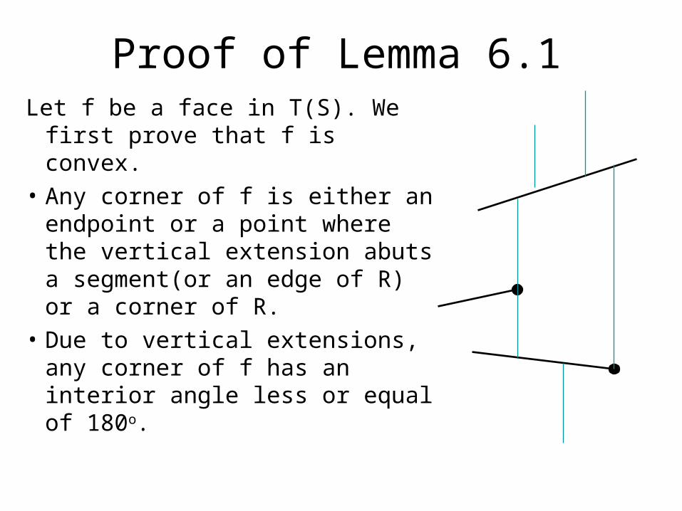
Proof of Lemma 6.1Let f be a face in T(S). We first

prove that f is convex.• Any corner of f is either an

endpoint or a point where the vertical extension abuts a segment(or an edge of R) or a corner of R.

• Due to vertical extensions, any corner of f has an interior angle less or equal of 180o.

Proof of Lemma 1(cont.)

• The convexity of f implies that it can have at most two vertical sides

• f cannot have more that two non-vertical sides, because otherwise they will meet in edge point and thus will be separated by vertical line through this point.

• f is bounded, thus it has exactly two non-vertical sides and at least one vertical side.

Notations

• Let top(D) (bottom(D)) be the segment of S, or edge of R, bounding the trapezoid D from above (below).

• Let denote the endpoint defining the left(right) edge by leftp(D) (rightp(D)).

• Notice that D is uniquely determined by top(D), bottom(D), leftp(D) and rightp(D).

Notations, Examples

D

rightp(D)

leftp(D)

top(D)

bottom(D)

top(D)

D

rightp(D)

bottom(D)

leftp(D)

Trapezoidal Maps, Complexity

Lemma 2: The trapezoidal map T(S) of a set of n line segments in general position contains at most 6n+4 vertices and at most 3n+1 trapezoids.

Proof of Lemma 2

• A vertex of T(S) is either a vertex of R, an endpoint of a segment in S, or else the point where the vertical extension starting at endpoint abuts on another segment or at boundary of R.

• Thus the total number of vertices in T(S) is bounded by:

4+2n+2(2n) = 6n+4

Proof of Lemma 2 (cont.)

• Each trapezoid, D, has a point leftp(D).

• Lets count the possible number of leftp().

• In the case of ambiguity consider leftp(D) as a point of bottom(D) or top(D) segments whenever possible.

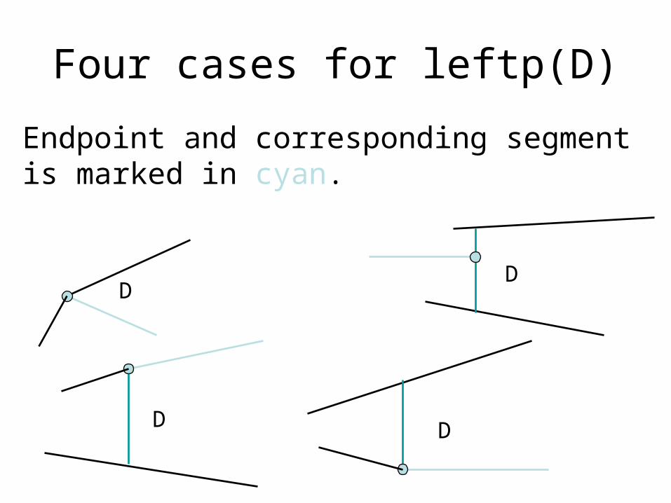
Four cases for leftp(D)

D

D

D

D

Endpoint and corresponding segment is marked in cyan.

Non-trivial case

• In case of leftp(D) lying on both top(D) and bottom(D), consider leftp(D) as an endpoint of bottom(D).

leftp()

Proof of Lemma 2 (cont.)

Thus right endpoint of any segment can be leftp() of only one trapezoid, and left endpoint of any segment can be leftp() of maximum two trapezoids. The lower left corner of R is a leftp() of exactly one trapezoid.

It follows that the total number of trapezoids is bounded by 3n+1.

Adjacent Trapezoids

• We call two trapezoids D, D` adjacent if they meet along a vertical edge.

• For set of points in general position a trapezoid has at most four adjacent trapezoids.

D

D1

D2

D3

D4

D5

Trapezoidal Map, Representation

• We use a specialized structure that uses the adjacency of trapezoids to link the subdivision as a whole.

• The structure contains records for trapezoids in T(S).

• The record for trapezoid D stores pointers to top(D),bottom(D),leftp(D),rightp(D) and pointers to its at most four neighbors.

A Randomized Incremental Alg. • In this section we will develop a

randomized incremental algorithm that constructs the trapezoidal map T(S) .

• During the construction the algorithm also builds a data structure D that can be used to perform point location queries in T(S).

• This is not a sweep line algorithm, because it doesn’t builds the data structure for queries

Desired Data Structure

• Directed acyclic graph with a single root

• Exactly one leaf for every trapezoid in trapezoid map of S

• Every inner node have out-degree 2

• 2 types of inner nodes:– x-nodes are labeled with an end-point of

some segment in S– y-nodes are labeled by segment itself

Example

The trapezoidal map of two segments an its’ search structure

p1

p1

A CF

D

B

E G

q1

q2

p2

s1

s2

A

s1

q1

q2

p2s2

C

B

D

E

F

Gs2

Algorithm TrapezoidalMap(S)

• Input: A set S of n non-crossing line segments• Output: The trapezoidal map T(S) and a search

structure D for T(S) in a bounding box

1. Determine a bounding box R that contains all segments of S, and initialize the trapezoidal map T and search structure D for it

2. Compute a random permutation s1,s2,…,sn of the elements of S

…

Alg. TrapezoidalMap(S) (cont...)3. for i <-- 1 to n

4. do Find the set 0,,…,k of trapezoids in T properly intersected by si

5. Remove 0,1,…,k from T and replace them by the new trapezoids that appear because of the intersection of si

6. Remove the leaves for 0,1,…,k from D, and create leaves for the new trapezoids. Link the new leaves to the existing inner nodes by adding some new inner nodes as explained below.

Detailed description of Alg.

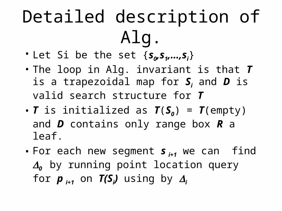
• Let Si be the set {s0,s1,…,si}• The loop in Alg. invariant is that T is a

trapezoidal map for Si and D is valid search structure for T

• T is initialized as T(S0) = T(empty) and D contains only range box R a leaf.

• For each new segment s i+1 we can find 0 by running point location query for p i+1 on T(Si) using by i

Example

0

1

3

2

p

qs

Alg. FollowSegment(T,si)

• Input: A trapezoidal map T, and a new segment si.

• Output: The sequence 0,1,…,k of trapezoids

intersected by si.

1. Let p and q be a left and right endpoints of si.

2. Search with p in the search structure to find 0.

3. j <-- 0

…

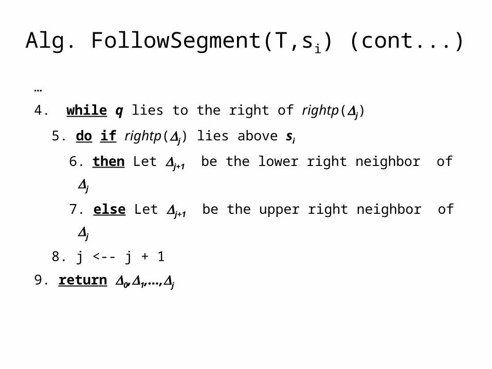
Alg. FollowSegment(T,si) (cont...)

…

4. while q lies to the right of rightp(j)

5. do if rightp(j) lies above si

6. then Let j+1 be the lower right neighbor of j

7. else Let j+1 be the upper right neighbor of j

8. j <-- j + 1

9. return 0,1,…,j

Updating T and D

• Let’s start with simple case that si is completely contained in trapezoid =0

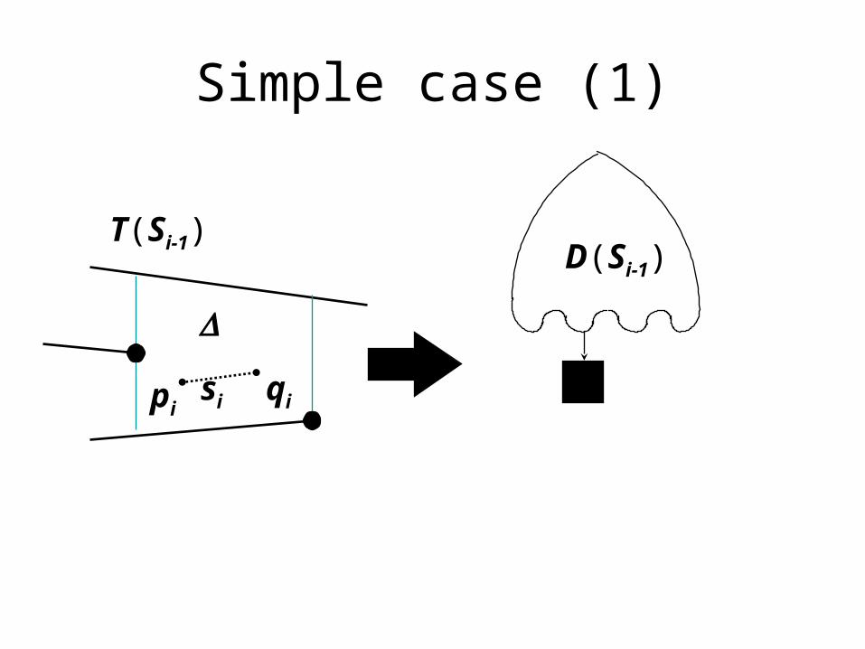
Simple case (1)

T(Si-1)

pi qisi

D(Si-1)

Simple case (2)Simple case (2)

T(Si)

C

D(Si)

pi

A

si

qi

B

CD

A BD

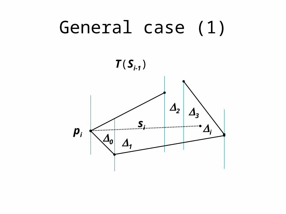
General case (1)

0 1

2 3pi i

si

T(Si-1)

General case (2)General case (2)

B C

D E

pi Fsi

T(Si)

A

General case (3)

D(Si-1)

1 2 3

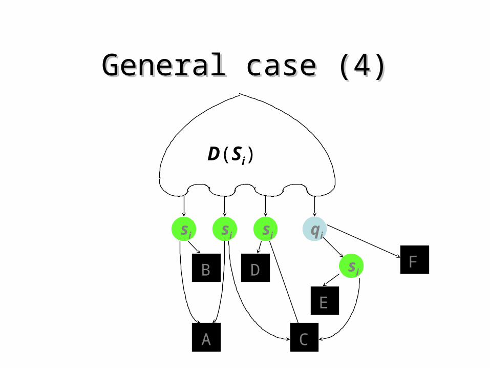
General case (4)General case (4)

D(Si)

A

si qi

C

B D

E

Fsi

si si

Theorem 3

Algorithm TrapezoidalMap computes the trapezoidal map T(S) of set S of n line segments in general position and a search structure D for T(S) in O(n log(n)) expected time. The expected size of the search structure is O(n) and for query point q the expected query time is O(log(n))

Proof of theorem 3 (1)

• 3 parts in this theorem will be proved– expected time of T(S) and D for T(S) building– expected size of D – expected time of query for given query point q

• Proof using by backward analysis

Proof of theorem 3 (2)• Let’s start with the query time of search

structure D for a fixed query point q.• The query time is equal to the length of the

search path for q in D. Thus it’s necessary to bound the length of search path.

• As we already observed every step in TrapezoidalMap algorithm adds maximum 3

levels into D structure. Hence, 3n is the upper bound on the query time for q.

Proof of theorem 3 (3)• We are interested in an expected time as well

as not in worst cases.• Let Xi, for 1<=i<=n, denote the number of nodes

on the query path created in iteration i. Since we consider S and q to be fixed, Xi is a random variable - it depends on the order of segments only.

• The expected path length is n n E[Xi] = E[Xi]

i=1 i=1

Proof of theorem 3 (4)

• We already saw that in any iteration alg. adds at most 3 nodes on the search path, so Xi <= 3.

• Let’s Pi denotes the probability that there exists the node on a search path of q that is created in iteration i

•E[Xi] <= 3Pi

Proof of theorem 3 (5)• Iteration i contributes a node to a search path of

q exactly if q(Si-1), the trapezoid containing q in T(Si-1), is no the same as q(Si)

Pi = Pr[q(Si-1) not the same as q(Si)]

• If q(si-1) not the same as q(si), then q(si) must be one of the trapezoids created in iteration i.

• Note that all trapezoids created in iteration I are adjacent to si : either top() or bottom() is si, or leftp() or rightp() as an endpoint of si

Proof of theorem 3 (6)

• Backward analysis: consider a fixed set Si as a subset of S. The T(Si) and q(si) defined as function of S and does not depend on the order in which segments of Si were inserted.

• Let’s compute the probability that q(si) disappear as a result of removing a random segment si from the Si. It disappears iff si is either top() or bottom() is si, or leftp() or rightp() as an endpoint of si

Proof of theorem 3 (7)• The probability that top() or bottom() is si, is at

most 1/i for each case. • leftp() disappears only if si is the only segment in

Si with leftp() as endpoint. Hence the probability that leftp() disappears is at most 1/i as well.

• Hence we can conclude that:

Pi=Pr[q(Si-1) not the same as q(Si)] =

Pr[q(Si) not belong to (Si-1) ] <= 4/i

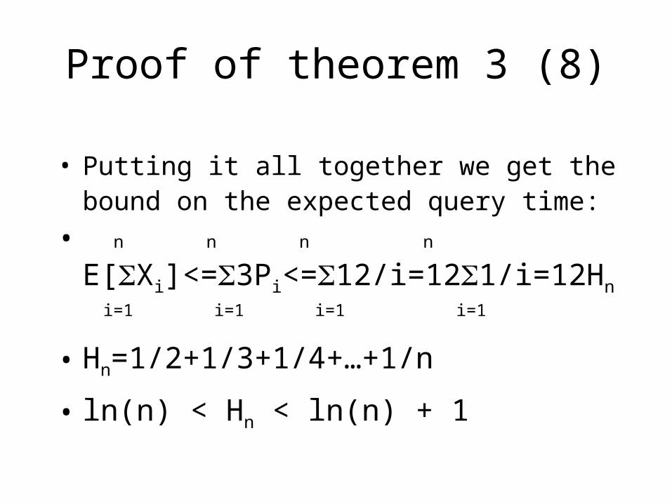
Proof of theorem 3 (8)

• Putting it all together we get the bound on the expected query time:

• n n n n

E[Xi]<=3Pi<=12/i=121/i=12Hn

i=1 i=1 i=1 i=1

• Hn=1/2+1/3+1/4+…+1/n

• ln(n) < Hn < ln(n) + 1

Proof of theorem 3 (9)• Now we will compute the bound size of D.• Each leaf in D corresponding one to one with trapezoid in

T(S), of which there are O(n) (see Lemma 2) • The total number of nodes in D is bounded by

n

O(n)+(number of inner nodes created by iter. i) i=1

• Let ki be a number of trapezoids created in iter. i. The number of inner nodes created in the same iter. is ki - 1. Hence: n n

O(n)+E[(ki-1)] = O(n)+E[ki] i=1 i=1

Proof of theorem 3 (10)• Consider a fixed set Si as a subset of S. for a trapezoid

and segment s from Si let:• 1 if disappears from T(Si) when si is removed from Si

(,s) := { 0 otherwise

• In the analysis of the query time we observed that here are at most 4 segments that cause a given trapezoid to disappear

• d(,s) <= 4|T(Si)| = O(i)s in Si in T(Si)

• Now , ki is the number of trapezoids created by insertion of si, or, equivalently the number of trapezoids in T(Si) that disappears when si removed.

Proof of theorem 3 (11)

• Since si is a random element in Si we can find the

expected value of Ki by the taking average over all s

in Si:

• E[ki]=1/i* d(,s)<= O(i)/i = O(1) s in Si in T(Si)

• We conclude that expected number of new inner nodes created in each iteration is O(1), from which O(n) bound on the expected size of D.

Proof of theorem 3 (12)

• To bound the expected running time of Alg. we only need to observe that the time to insert segment si is O(ki) plus the time needed to locate the left endpoint of si in T(Si-1). Thus the time bound is :

• n

O(1) + {O(logn) + O(E[ki])} = O(nlogn) i=1

Dealing with degenerate cases• Symbolic shear transformation(x , y) = (x + y , y)

• Given a set S of n arbittrary non-crossing line-segments, we will run algorithm TrapezoidalMap on the set S := { s : s from S }.

Dealing with degenerate cases

• To reduce probability of numerical problems in transformation every point (p) = (x + y , y) will simply be stored as (x,y). We only need to make sure that the Alg. treats this data correctly.

• 2 types of elementary operation on input points

Dealing with degenerate cases

The first operation tkes 2 distinct points p and q and desides whether q lies to the left, to the right, or on the vertical line throught p.

The second oeration takes one of the input segments and tests wheter q lies above, below or on this segment.

Tail Estimate

In previous theorem it was proved that expected query time is O(log n). This is a rather weak result. In fact, there’s no reason to expect that maximum query time of the search structure is small.

In this sections we shall prove that probability that search structure has a bad query time for some query point is very small.

Lemma 6

Let S be a set of n non-crossing line segments, let q be a query point, and let a be a parameter with a > 0. Then the probability that the search path for q in the search structure computed by Algorithm TrapezoidalMap has more than 3 a ln(n+1) nodes is at most 1/(n+1)a ln 1.25 - 1.

Proof of Lemma 6 (1)

• We would like to define random variables Xi, with 1 <= i <= n, such that Xi = 1 if at least one node on the search path for q has been created on iteration i.

• Unfortunately, the random variables created this way are not independent. We didn’t need independence in the Proof of Theorem 3, but we shall need it here.

• Lets use a little trick!

Proof of Lemma 6 (2)

• We define a directed acyclic graph G, with one source and one sink. Paths from source to sink correspond to permutations in S.

• There’s a node for every subset of S, including one for the empty set.

• A subset S` of cardinality i has outgoing edge to the subset S`` of cardinality i+1, if S`` contains S` and edge is associated with segment S``\S`.

Permutation Graph

• It is convenient to imagine the nodes as being grouped into n+1 layers, such that layer i contains the subsets of cardinality i.

{1,2,3,4}

{1,2,3} {2,3,4}

{}

{1} {4}

{1,2} {3,4}

1 4

2

3

4

3

2

1

Proof of Lemma 6 (3)• Directed paths from the source to the sink in G now

correspond one-to-one to permutations of S, which correspond to possible executions of algorithm TrapezoidalMap.

• Lets mark the edge if this insertion changes the trapezoid containing point q.

• By backward analysis we get that any node in G has at most four marked incoming edges.

• If a node has less than four marked edges, mark more edges arbitrary, to total 4 marked.

Proof of Lemma 6 (4)

• Lets define an indicator Xi, Xi=1 iff the i-th edge on the sink-to-source path in G is marked.

• Since each node in layer i has i incoming edges, exactly four of which are marked (assuming i>3), this implies that Pr[Xi=1]=4/i for i>3, and Pr[Xi=1]=1 for i<=3.

• Note that Xi are independent.

Proof of Lemma 6 (5)

• Let Y = sum Xi. The number of nodes in the search path for q is at most 3Y. Lets bound the probability that Y exceeds a ln(n+1).

• We use Markov’s inequality:For any non-negative random variable Z and any a > 0

Pr[ ]E[ ]

Z aZ

a

Proof of Lemma 6 (6)

• So for any t > 0 we have

• Recall that expected value of the sum of random variables is the sum of the expected values and for independent random variables expected product is the product of expected values, so we have:

Pr[ ln( )] Pr[ ] E[ ]ln( ) ln( )Y a n e e e etY ta n ta n tY 1 1 1

E[ ] E[ ] E[ ] E[ ]e e e etY tX tX

i

tX

i

ii i i

Proof of Lemma 6 (7)

• and if we choose t = ln 1.25, we get

• and we have:

E e ei

ei

i i ii

i

tX ti[ ] ( )

( / )

41

4

1 1 44

14

11 1

0

E en

nntX

i

ni[ ]

1

21

32

11

Proof of Lemma 6 (8)

Putting everything together, we get the bound we want to prove:

Pr[ ln( )]

( )( )

/ ( )ln( )

Y a n

e nn

nnat n

atat

1

11

11 11 1

Lemma 7

Let S be the set of n non-crossing line segments, and let a be a parameter a > 0. Then the probability that the depth of the search structure computed by Algorithm TrapezoidalMap for S is more than 3 a ln(n+1) is at most 2/(n+1)(a ln1.25-3).

Proof of Lemma 7• We will call two query points q and q`

equivalent if they follow the same path through the search structure D.

• Recall partition the plane into vertical slabs. This defines a decomposition of the plane into at most 2(n+1)2 trapezoids

• Any two points lying in the same trapezoid in this decomposition must be equivalent in every possible structure for S.

Proof of Lemma 7 (cont.)

• Thus the depth of D is the maximum of the length of the search path for at most 2(n+1)2 query points.

• By Lemma 6 the probability that length of search path for fixed point q exceeds 3 a ln(n+1) is at most 1/(n+1)(a ln 1.25 -1)

• Thus the probability that length of the search path for any one of 2(n+1)2 test points exceeds the bound is therefore at most: 2(n+1)2/(n+1)(a ln 1.25 - 1) = 2/(n+1)(a ln 1.25 -3)

Discussion of proved results

• Lemma 7 implies that expected maximum query time is O(log n).

• Take a = 20, then a probability that the depth of D is more than 3 a ln(n+1) is at most 2/(n+1)1.4 which is less than 1/4 for n>4.

• Similarly, the size of D is O(n) and construction time is O(n log n) with probability at lest 3/4.

Main result

Theorem 8: Let S be a planar subdivision with n edges. There exists a point location data structure for S that uses O(n) storage and has O(log n) query time in the worst case. The structure can be build inO(n log n) expected time.

The Algorithm

• Run algorithm TrapezoidalMap on the set S, keeping track of the search structure that is being created.

• As soon as size exceeds c1*n or depth exceeds c2*log n for suitably chosen constants c1 and c2, stop the algorithm and start it with another permutation.

• Since the probability of good permutation is 1/4 (a=20) so we expect to finish in 4 trials.

Summary

• We learned an algorithm for point location problem.

• An algorithm in O(n log n) expected time creates a search structure of size O(n), which is capable to answer point location queries in O(log n) time.

The End

Another approach -persistency

• Recall the slabs subdivision.• The problem is that we hold a tree for each

slab, so we get O(n2) space.• But the structure of trees in the adjacent

slabs are almost identical.• Idea: Do not hold the new trees, but only the

changes of the previous(from left to right)• Result: O(n) space,with same O(log n) time.