pointwise green's function approach to stability for scalar conservation laws

Pointwise Green’s Function Approach to Stabilityfor Scalar Conservation Laws

PETER HOWARDIndiana University

Abstract

We study the pointwise behavior of perturbations from a viscous shock solutionto a scalar conservation law, obtaining an estimate independent of shock strength.We find that for a perturbation with initial data decaying algebraically or slower,the perturbation decays in time at the rate of decay of the integrated initial datain anyLp norm,p≥ 1. Stability in anyLp norm is a direct consequence. The ap-proach taken is that of obtaining pointwise estimates on the perturbation througha Duhamel’s principle argument that employs recently developed pointwise es-timates on the Green’s function for the linearized equation.c© 1999 John Wiley& Sons, Inc.

1 Introduction

We consider the scalar viscous conservation law

ut + f (u)x = uxx, f ,u,x∈ R, t ∈ R+ , u(0,x) = u0(x) ,(1.1)

wheref ∈C2(R) andu0(x)→ u± asx→±∞. Physical contexts in which equationsof form (1.1) arise are discussed, for example, in [9]. We will be concerned withtraveling wave solutionsto (1.1), that is, solutions of the form ¯u(x−st) that satisfyu(±∞) = u± and the Rankine-Hugoniot condition

s(u+−u−) = f (u+)− f (u−) .

We note that by a translation of coordinates we may takes = 0 without loss ofgenerality. In particular, we will consider Lax shocks, that is,u satisfying f ′(u+) <s< f ′(u−). In the scalar case with diffusion only, this just rules outsonicshocksfor which f ′(u−) or f ′(u+) is equal tos.

The result obtained is a pointwise estimate on perturbations from viscous pro-file solutions to (1.1), an estimate that agrees with the exact analysis of Burgers’equation carried out by Nishihara [18]. From our estimate, nonlinear orbital stabil-ity follows in anyLp norm,p≥ 1. Our key observation is a precise formulation ofhow spatial decay of initial data leads directly to temporal decay of the perturba-tion. Nishihara observed this fact for Burgers’ equation and general algebraicallydecaying data, and Liu [11] observed it forn-dimensional systems of conserva-tion laws for weak shocks and data decaying as(1+ |x|)−3/2. A method by whichthe constant diffusion term in our analysis may be replaced by the more general(b(u)ux)x (whereb(u) > b0 > 0 andb∈C1+α, α > 0) is given in [23] but not em-ployed here.

Communications on Pure and Applied Mathematics, Vol. LII, 1295–1313 (1999)c© 1999 John Wiley & Sons, Inc. CCC 0010–3640/99/101295-19

1296 P. HOWARD

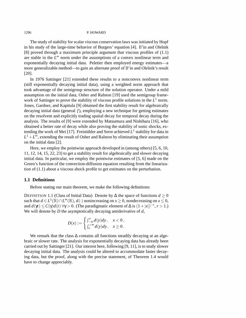
The study of stability for scalar viscous conservation laws was initiated by Hopfin his study of the large-time behavior of Burgers’ equation [4]. Il’in and Oleınik[8] proved through a maximum principle argument that viscous profiles of (1.1)are stable in theL∞ norm under the assumptions of a convex nonlinear term andexponentially decaying initial data. Peletier then employed energy estimates—amore generalizable method—to gain an alternate proof of Il’in and Oleınik’s result[20].

In 1976 Sattinger [21] extended these results to a nonconvex nonlinear term(still exponentially decaying initial data), using a weighted norm approach thattook advantage of the semigroup structure of the solution operator. Under a mildassumption on the initial data, Osher and Ralston [19] used the semigroup frame-work of Sattinger to prove the stability of viscous profile solutions in theL1 norm.Jones, Gardner, and Kapitula [9] obtained the first stability result for algebraicallydecaying initial data (generalf ), employing a new technique for getting estimateson the resolvent and explicitly trading spatial decay for temporal decay during theanalysis. The results of [9] were extended by Matsumura and Nishihara [16], whoobtained a better rate of decay while also proving the stability of sonic shocks, ex-tending the work of Mei [17]. Freistühler and Serre achievedL1 stability for data inL1+L∞, extending the result of Osher and Ralston by eliminating their assumptionon the initial data [2].

Here, we employ the pointwise approach developed in (among others) [5, 6, 10,11, 12, 14, 15, 22, 23] to get a stability result for algebraically and slower decayinginitial data. In particular, we employ the pointwise estimates of [5, 6] made on theGreen’s function of the convection-diffusion equation resulting from the lineariza-tion of (1.1) about a viscous shock profile to get estimates on the perturbation.

1.1 Definitions

Before stating our main theorem, we make the following definitions:

DEFINITION 1.1 (Class of Initial Data) Denote by∆ the space of functionsd ≥ 0such thatd∈ L1(R)∩L∞(R), d(·) nonincreasing onx≥ 0, nondecreasing onx≤ 0,andd(γt)≤C(γ)d(t) ∀γ > 0. (The paradigmatic element of∆ is (1+ |x|)−r , r > 1.)We will denote byD the asymptotically decaying antiderivative ofd,

D(x) :=

{∫ x−∞ d(y)dy, x < 0,∫ +∞x d(y)dy, x≥ 0.

We remark that the class∆ contains all functions steadily decaying at an alge-braic or slower rate. The analysis for exponentially decaying data has already beencarried out by Sattinger [21]. Our interest here, following [9, 11], is to study slowerdecaying initial data. The analysis could be altered to accommodate faster decay-ing data, but the proof, along with the precise statement, of Theorem 1.4 wouldhave to change appreciably.

POINTWISE APPROACH TO STABILITY 1297

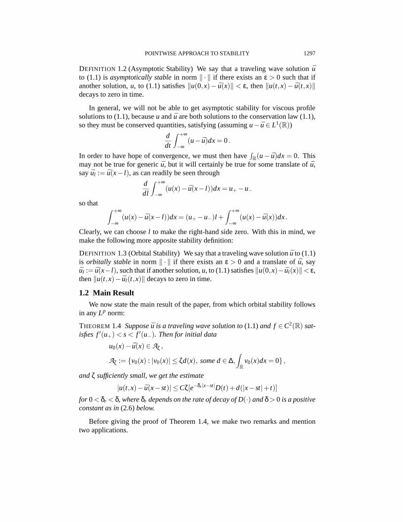
DEFINITION 1.2 (Asymptotic Stability) We say that a traveling wave solution ¯uto (1.1) isasymptotically stablein norm ‖ · ‖ if there exists anε > 0 such that ifanother solution,u, to (1.1) satisfies‖u(0,x)− u(x)‖ < ε, then‖u(t,x)− u(t,x)‖decays to zero in time.

In general, we will not be able to get asymptotic stability for viscous profilesolutions to (1.1), becauseu andu are both solutions to the conservation law (1.1),so they must be conserved quantities, satisfying (assumingu− u∈ L1(R))

ddt

∫ +∞

−∞(u− u)dx= 0.

In order to have hope of convergence, we must then have∫R(u− u)dx= 0. This

may not be true for generic ¯u, but it will certainly be true for some translate of ¯u,sayul := u(x− l), as can readily be seen through

ddl

∫ +∞

−∞(u(x)− u(x− l))dx= u+−u−

so that ∫ +∞

−∞(u(x)− u(x− l))dx= (u+−u−)l +

∫ +∞

−∞(u(x)− u(x))dx.

Clearly, we can choosel to make the right-hand side zero. With this in mind, wemake the following more apposite stability definition:

DEFINITION 1.3 (Orbital Stability) We say that a traveling wave solution ¯u to (1.1)is orbitally stablein norm ‖ · ‖ if there exists anε > 0 and a translate of ¯u, sayul := u(x− l), such that if another solution,u, to (1.1) satisfies‖u(0,x)− ul(x)‖< ε,then‖u(t,x)− ul (t,x)‖ decays to zero in time.

1.2 Main ResultWe now state the main result of the paper, from which orbital stability follows

in anyLp norm:

THEOREM 1.4 Supposeu is a traveling wave solution to(1.1)and f ∈C2(R) sat-isfies f′(u+) < s< f ′(u−). Then for initial data

u0(x)− u(x) ∈ Aζ ,

Aζ := {v0(x) : |v0(x)| ≤ ζd(x), some d∈ ∆,

∫R

v0(x)dx= 0} ,

andζ sufficiently small, we get the estimate

|u(t,x)− u(x−st)| ≤Cζ[e−δr |x−st|D(t)+d(|x−st|+ t)]

for 0< δr < δ, whereδr depends on the rate of decay of D(·) andδ > 0 is a positiveconstant as in(2.6)below.

Before giving the proof of Theorem 1.4, we make two remarks and mentiontwo applications.

1298 P. HOWARD

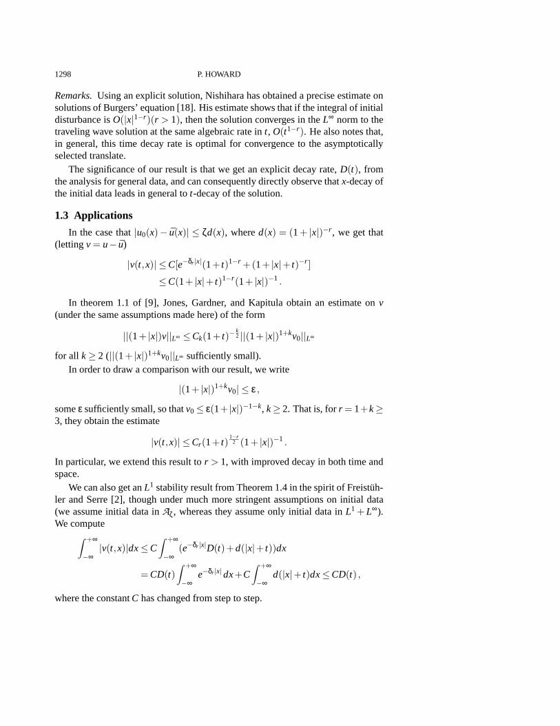
Remarks.Using an explicit solution, Nishihara has obtained a precise estimate onsolutions of Burgers’ equation [18]. His estimate shows that if the integral of initialdisturbance isO(|x|1−r)(r > 1), then the solution converges in theL∞ norm to thetraveling wave solution at the same algebraic rate int, O(t1−r). He also notes that,in general, this time decay rate is optimal for convergence to the asymptoticallyselected translate.

The significance of our result is that we get an explicit decay rate,D(t), fromthe analysis for general data, and can consequently directly observe thatx-decay ofthe initial data leads in general tot-decay of the solution.

1.3 Applications

In the case that|u0(x)− u(x)| ≤ ζd(x), whered(x) = (1+ |x|)−r , we get that(lettingv = u− u)

|v(t,x)| ≤C[e−δr |x|(1+ t)1−r +(1+ |x|+ t)−r ]

≤C(1+ |x|+ t)1−r(1+ |x|)−1 .

In theorem 1.1 of [9], Jones, Gardner, and Kapitula obtain an estimate onv(under the same assumptions made here) of the form

||(1+ |x|)v||L∞ ≤Ck(1+ t)−k2 ||(1+ |x|)1+kv0||L∞

for all k≥ 2 (||(1+ |x|)1+kv0||L∞ sufficiently small).In order to draw a comparison with our result, we write

|(1+ |x|)1+kv0| ≤ ε ,

someε sufficiently small, so thatv0 ≤ ε(1+ |x|)−1−k, k≥ 2. That is, forr = 1+k≥3, they obtain the estimate

|v(t,x)| ≤Cr(1+ t)1−r

2 (1+ |x|)−1 .

In particular, we extend this result tor > 1, with improved decay in both time andspace.

We can also get anL1 stability result from Theorem 1.4 in the spirit of Freistüh-ler and Serre [2], though under much more stringent assumptions on initial data(we assume initial data inAζ, whereas they assume only initial data inL1 + L∞).We compute∫ +∞

−∞|v(t,x)|dx≤C

∫ +∞

−∞(e−δr |x|D(t)+d(|x|+ t))dx

= CD(t)∫ +∞

−∞e−δr |x| dx+C

∫ +∞

−∞d(|x|+ t)dx≤CD(t) ,

where the constantC has changed from step to step.


Further, we note that for any 1< p < ∞, we get∫ +∞

−∞|v|pdx≤C

∫ +∞

−∞(e−δr |x|D(t)+d(|x|+ t))pdx

≤C(D(t)+d(t))p−1∫ +∞

−∞(e−δr |x|D(t)+d(|x|+ t))dx

≤C(D(t)+d(t))p−1D(t) ≤CD(t)p .

Hence we arrive at the estimate(∫ +∞

−∞|v|pdx

)1/p ≤CD(t) .

Thus, forv ∈ Aζ, the decay rate ofv in Lp for any 1 ≤ p ≤ ∞ is againD(t) (cf.corollary 1.2 of [11]).

1.4 Plan of the Paper

In Section 2 we give an outline of the general procedure based on [15, 23],reducing the proof of Theorem 1.4 to gaining tight estimates on certain Duhamelintegrals. In Section 3 we carry out the analysis by obtaining the necessary esti-mates.

2 General Procedure

We begin by letting ¯u(x−st) denote a traveling wave solution to (1.1). Lettingu = u+v be another solution, our goal will be to obtain pointwise estimates on theperturbationv.

First, we choose a translate of ¯u (renamed ¯u for convenience) so that (see dis-cussion after Definition 1.2) ∫ +∞

−∞(u− u)dx= 0.

Substitutingu = u+v into (1.1), we arrive at the linearized equation forv

vt +( f ′(u)v)x = vxx+O(v2)x .(2.1)

We now make the changew(·,x) =∫ x−∞ v(·,ξ)dξ. Note that we have chosen our

profile so that∫ +∞−∞ v(·,ξ)dξ = 0, giving∫ x

−∞v(·,ξ)dξ = −

∫ +∞

xv(·,ξ)dξ ,

and so we also have thatw(0,x) = −∫ +∞x v(0,ξ)dξ. In the following analysis, we

will mean by∫ xv(0,ξ)dξ whichever representation is most useful.

Integrating (2.1) from−∞ to x, we get∫ x

−∞vt(t,ξ)dξ+ f ′(u)v(t,x) = vx(t,x)+O(v2)

1300 P. HOWARD

or

wt + f ′(u)wx = wxx+O(v2) ,

the integrated form of (2.1). We note that the big O term is left as a function ofv2

for later convenience.The need to work with the integrated equation is a consequence of the pointwise

Green’s function estimates in [5, 6] holding only in situations for which there areno eigenvalues (point spectrum) at the origin. In the Lax case for the nonintegratedequation, there is an eigenvalue at the origin. In the integrated case, however, thereis never an eigenvalue at the origin, as is easy to see through a direct computation.

We remark that this eigenvalue at the origin is a permanent fixture of viscousconservation laws, and that in general (in the case of higher-order scalar equationsand systems of any order) this eigenvalue cannot be projected out (integrated out).In these cases, a similar analysis maintains, in which the eigenvalue is taken intoaccount through a residue analysis (see [7] for the case of higher-order scalar equa-tions and [23] for the case of systems).

Define now the linear operator

Lw := wxx− ( f ′(u)w) .

With a(x) := f ′(u), theorem 1.1 of [6] (see Proposition 2.2 below) gives bounds onthe Green’s function,G(t,x;y), for

wt = Lw.(2.2)

What we are interested in here, however, is the forced equation

wt −Lw = O(v2) .(2.3)

Applying Duhamel’s principle to (2.3), we get

w(t,x) = eLtw(0,x)+∫ t

0eL(t−s)O(v2)(s,x)ds

=∫ +∞

−∞G(t,x;y)w(0,y)dy+

∫ t

0

∫ +∞

−∞G(t −s,x;y)O(v2)(s,y)dyds.

We now take anx-derivative of this integral equation to arrive at

wx(t,x) =∫ +∞

−∞Gx(t,x;y)w(0,y)dy

+∫ t

0

∫ +∞

−∞Gx(t −s,x;y)O(v2)(s,y)dyds.

Writing the above integral equation again in terms ofv yields

v(t,x) =∫ +∞

−∞Gx(t,x;y)

∫ yv(0,ξ)dξdy

+∫ t

0

∫ +∞

−∞Gx(t −s,x;y)O(v2)(s,y)dyds.


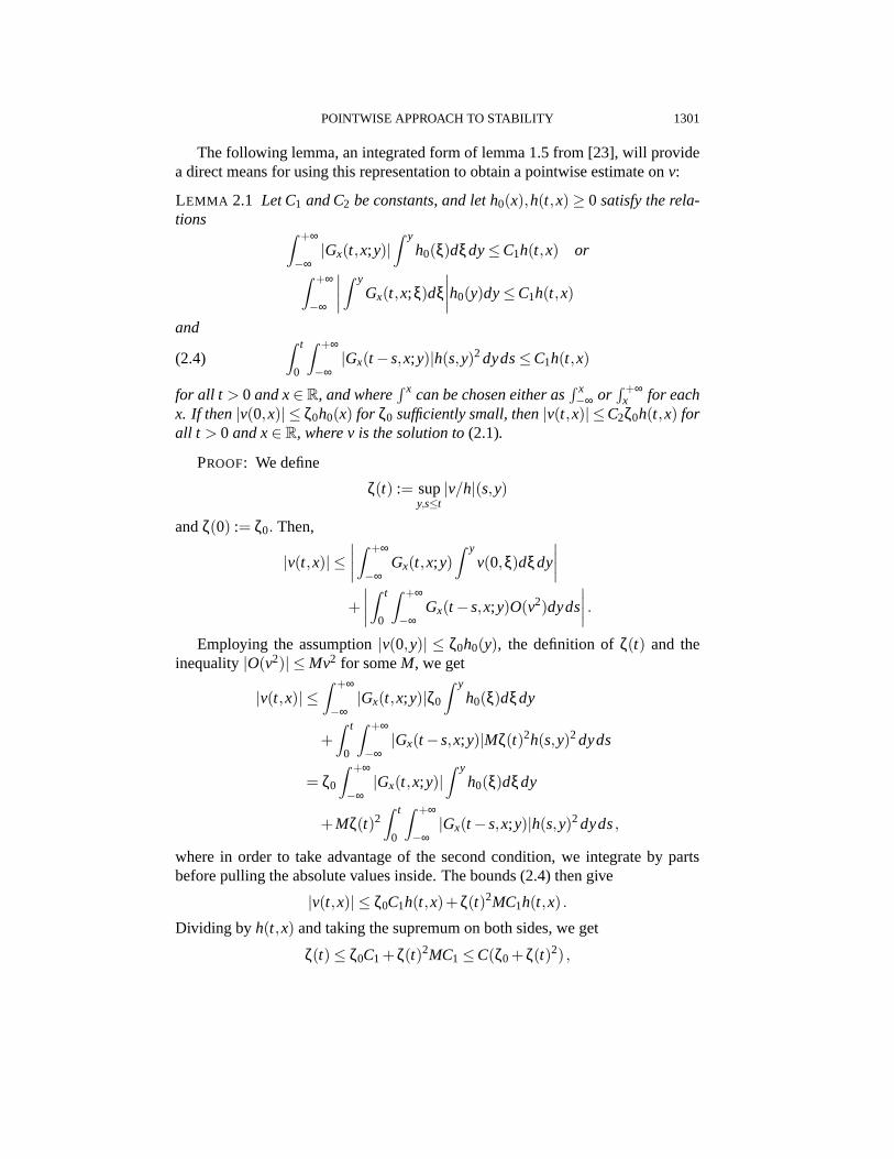
The following lemma, an integrated form of lemma 1.5 from [23], will providea direct means for using this representation to obtain a pointwise estimate onv:

LEMMA 2.1 Let C1 and C2 be constants, and let h0(x),h(t,x) ≥ 0 satisfy the rela-tions ∫ +∞

−∞|Gx(t,x;y)|

∫ yh0(ξ)dξdy≤C1h(t,x) or

∫ +∞

−∞

∣∣∣∣∫ y

Gx(t,x;ξ)dξ∣∣∣∣h0(y)dy≤C1h(t,x)

and ∫ t

0

∫ +∞

−∞|Gx(t −s,x;y)|h(s,y)2dyds≤C1h(t,x)(2.4)

for all t > 0 and x∈ R, and where∫ x can be chosen either as

∫ x−∞ or

∫ +∞x for each

x. If then|v(0,x)| ≤ ζ0h0(x) for ζ0 sufficiently small, then|v(t,x)| ≤C2ζ0h(t,x) forall t > 0 and x∈ R, where v is the solution to(2.1).

PROOF: We define

ζ(t) := supy,s≤t

|v/h|(s,y)

andζ(0) := ζ0. Then,

|v(t,x)| ≤∣∣∣∣∫ +∞

−∞Gx(t,x;y)

∫ yv(0,ξ)dξdy

∣∣∣∣+

∣∣∣∣∫ t

0

∫ +∞

−∞Gx(t −s,x;y)O(v2)dyds

∣∣∣∣ .Employing the assumption|v(0,y)| ≤ ζ0h0(y), the definition ofζ(t) and the

inequality|O(v2)| ≤ Mv2 for someM, we get

|v(t,x)| ≤∫ +∞

−∞|Gx(t,x;y)|ζ0

∫ yh0(ξ)dξdy

+∫ t

0

∫ +∞

−∞|Gx(t −s,x;y)|Mζ(t)2h(s,y)2dyds

= ζ0

∫ +∞

−∞|Gx(t,x;y)|

∫ yh0(ξ)dξdy

+Mζ(t)2∫ t

0

∫ +∞

−∞|Gx(t −s,x;y)|h(s,y)2dyds,

where in order to take advantage of the second condition, we integrate by partsbefore pulling the absolute values inside. The bounds (2.4) then give

|v(t,x)| ≤ ζ0C1h(t,x)+ζ(t)2MC1h(t,x) .

Dividing by h(t,x) and taking the supremum on both sides, we get

ζ(t) ≤ ζ0C1 +ζ(t)2MC1 ≤C(ζ0 +ζ(t)2) ,

1302 P. HOWARD

whereC := max{C1,C1M}. Takingζ0 small enough so that 4C2ζ0 < 1, we applycontinuous inductionto show thatζ(t) ≤ 2Cζ0. That is, by the continuity ofζ(t),we can takeC large enough so that we havestrict inequality (ζ(t) < 2Cζ0) onsome sufficiently small intervalt ∈ [0,T]. LetT be the first time for which equalityoccurs (ζ(T) = 2Cζ0). If no suchT exists, we are done. If such aT does exist, wecompute

ζ(T) ≤C(ζ0 +ζ(T)2) = C(ζ0 +4C2ζ20) < Cζ0 +Cζ0 = 2Cζ0 .

This contradiction completes the proof.

We will achieve the estimates assumed in Lemma 2.1 through the pointwiseGreen’s function estimates of theorem 1.1 in [6], given below for the Lax case asProposition 2.2.

PROPOSITION2.2 Under the hypotheses of Theorem1.4, the Green’s function for

wt + f ′(u)wx = wxx,(2.5)

where a(x) := f ′(u) and a± := limx→±∞ a(x) in the Lax case(a+ < 0< a−) satisfiesthe estimate( for x≥ 0)

|Gx(t,x;y)| ≤

C1e−δ|x|√t

e−(x−y−a+t)2

Mt + C1t e−

(x−y−a+t)2

Mt , y≥ 0,

C1e−δ|x|√t

e−(x−y−a−t)2

Mt + C1e−δ|x|t e−

(x−y−a−t)2

Mt , y≤ 0,(2.6)

where we have subsumed certain constants into M and C1 (the subscript followsthe notation of [6] and is indicative of the first derivative), and where M, C1, andδ each depend upon the asymptotic behavior of f′(u(x)) and on the spectrum ofthe associated linearized operator L(defined above). Symmetric estimates hold forx≤ 0.

PROOF: As discussed in [6], the elliptic eigenvalue equation associated with(2.5) has no eigenvalues on or to the left of the imaginary axis. Further,f ∈C2(R)givesa∈C1(R), satisfying the assumptions needed in theorem 1.1 of [6] for first-order derivative estimates.

We note before proceeding that results similar to that of Proposition 2.2 can beobtained for a broad class of linear equations, including those obtained through thelinearization of higher-order scalar conservation laws [7], those obtained throughthe linearization of systems of conservation laws [23], and (through a somewhatsimilar analysis in a different setting) a very general class of second-order ellipticoperators with complex, bounded, measurable coefficients inR

n [1].In each of the cases arising from the analysis of conservation laws, the spectral

approach of [13] is employed and extended to the nonconstant coefficient casethrough the semigroup framework of [9, 21]. In particular, the analysis breaksinto two parts: a small-time/large-eigenvalue portion that follows the outline of aFourier transform analysis of the constant-coefficient evolution equation with only


the highest-order spatial derivative considered, and a large-time/small-eigenvalueportion that follows the outline of a Fourier transform analysis of the constant-coefficient evolution equation with only the lowest two-order spatial derivativesconsidered. The analysis of [1] is similar to the small-time analysis mentionedabove.

In the next section we find an appropriatetemplate function, h(t,x) (see [11, 14,15, 23]), and employ it to prove Theorem 1.4.

3 Proof of Theorem 1.4

In the scalar case with diffusion only, we only have a viscous profile when theLax entropy condition holds (f ′(u+) < s< f ′(u−) or with s= 0, a+ < 0< a−, thatis n+1 = 2 incoming characteristics). Without loss of generality (by symmetry ofthe estimates of Proposition 2.2), we may takex ≥ 0. The following lemma willgreatly simplify the forthcoming analysis:

LEMMA 3.1 Let f(y)≥ 0 be a nonincreasing function onR+, with f(0) < C1. As-sume further that there exist constantsγ > 0 andω > 1 so that f(y)≥ γe−

a2(1− 1

ω )2y2

onR+. Then, for a,z> 0∫ +∞

0e−a(z−y)2

f (y)dy≤ C(ω)√a

f (z/ω) .

Remark3.2. By symmetry we have forz< 0∫ 0

−∞e−a(z−y)2

f (y)dy≤ C(ω)√a

f (z/ω)

for ω < −1 and f nonincreasing onR− and satisfying the same lower bound asabove. Thispeak estimatecharacterizes how the kernel

√ae−a(z−y)2

behaves like adelta-function.

Remark3.3. Also convenient for the forthcoming analysis is the observation thatfor z≥ 0, y≤ 0, anda > 0, we have thetail estimate

∫ y

−∞e−a(z−ξ)2

dξ ≤ 12

√2πa

e−a2(z−y)2

,

with a symmetric result true forz≤ 0 andy≥ 0. This observation is easily recog-nized through the computation∫ y

−∞e−a(z−ξ)2

dξ =∫ y

−∞e−

a2(z−ξ)2− a

2(z−ξ)2dξ =

∫ y

−∞e−

a2(z−ξ)2

e−a2(z−ξ)2

dξ

≤ e−a2(z−y)2

∫ y

−∞e−

a2(z−ξ)2

dξ ≤ e−a2(z−y)2 1

2

√2πa

.

1304 P. HOWARD

PROOF OFLEMMA 3.1: We break the integration into two regions as follows:∫ +∞

0e−a(z−y)2

f (y)dy=∫ z/ω

0e−a(z−y)2

f (y)dy+∫ +∞

z/ωe−a(z−y)2

f (y)dy.(3.1)

We note that the result follows immediately for the second integral on the right-hand side of (3.1), since we can write∫ +∞

z/ωe−a(z−y)2

f (y)dy≤ f (z/ω)∫ +∞

x/ωe−a(z−y)2

dy≤ C√a

f (z/ω) .

For the first integral on the right-hand side of (3.1), we compute∫ z/ω

0e−a(z−y)2

f (y)dy≤ f (0)(z/ω)e−a(1− 1ω )2z2

≤ f (0)ω√a

e−a2(1− 1

ω )2z2 ≤ C(ω)√a

f (z/ω) ,

where we have used above thatze−a2(1− 1

ω )2z2 ≤C(ω)/√

a for some constantC(ω).This completes the proof.

We are now prepared to prove two lemmas regarding the behavior of elementsof ∆ integrated againstGx(t,x;y).

LEMMA 3.4 Under the assumptions of Theorem1.4 and with G(t,x;y) being theGreen’s function for(2.2), we have for d(x) ∈ ∆,∫ +∞

−∞|Gx(t,x;y)|

∫ yd(ξ)dξ dy≤C

[e−δr |x|D(t)+d(|x|+ t)

]or ∫ +∞

−∞

∣∣∣∣∫ y

Gx(t,x;ξ)dξ∣∣∣∣d(y)dy≤C

[e−δr |x|D(t)+d(|x|+ t)

]for 0 < δr < δ, whereδr depends on the rate of decay of D(·), δ is as in(2.6), and∫ y =

∫ y−∞ or

∫ +∞y .

Remark3.5. We will take advantage in the proof of Lemma 3.4 of the identity∫ +∞

−∞Gx(t,x;y)dy= 0

by using ∫ y

−∞Gx(t,x;ξ)dξ = −

∫ +∞

yGx(t,x;ξ)dξ .

This identity is clear from the relationship betweenG andG, the Green’s function

for the unintegrated problem, namely,Gx(t,x;y) d=Gy(t,x;y). We can see this asfollows: Letw solve the integrated equation andv the unintegrated equation so thatwt = Lw andvt = Lv, whereL is the spatial operator for the unintegrated equation


(2.1) (minus the error term). We then have thatw = G∗w0 andv = G∗ v0, wherew0 andv0 are initial data. Sincev = wx, we getv = Gx ∗w0, but sincew0y = v0,we also havev = G∗v0 = G∗w0y = Gy∗w0. Comparing gives the claim under

distribution, which is what we mean byd=.

PROOF OFLEMMA 3.4: Without loss of generality (by symmetry), we needonly concern ourselves with the casex≥ 0.

3.1 Large-Time Estimates

Assumet ≥ 1. In this case we can uset−1/2 ≤C(1+ t)−1/2. The estimate willfollow immediately in the casey≤ 0 from the additional exponential decay inx.

We compute∫ +∞

−∞|Gx(t,x;y)|

∫ yd(ξ)dξdy=

∫ 0

−∞|Gx(t,x;y)|D(y)dy+

∫ +∞

0|Gx(t,x;y)|D(y)dy.

For the integral overy≤ 0 we have a bound by∫ 0

−∞

C1e−δ|x|√

te−

(x−y−a−t)2

Mt D(y)dy+∫ 0

−∞

C1e−δ|x|

te−

(x−y−a−t)2

Mt D(y)dy.

We consider two cases:x ≥ εt andx ≤ εt for some 0< ε � a−. In the casethatx≥ εt, the exponentialx-decay also gives exponentialt-decay, better than ourclaimed estimate. In the casex≤ εt, we have thatx−a−t < 0, so that Remark 3.2applies, giving a bound by

C1e−δ|x|D(−x+a−t)+C1e−δ|x|t−1/2D(−x+a−t) ≤C1e−δ|x|D((a−− ε)t)+C1t

−1/2e−δ|x|D((a−− ε)t) .Note that here and in the following computations, we will use our assumption thatd is radial to keep the argument ofd andD positive.

We now consider the integral overy≥ 0, which, as above, is bounded by∫ +∞

0

[C1e−δ|x|

√t

e−(x−y−a+t)2

Mt +C1

te−

(x−y−a+t)2

Mt

]D(y)dy≤

C1e−δ|x|D(x+ |a+|t)+C1t−1/2D(x+ |a+|t) ,

where the inequality is an application of Lemma 3.1.We note that for the second term in the last expression we can do better. In fact,

as we need anL1 bound onv, we mustdo better. Motivated by the observationthat we would like to achieved(|x|+ t) decay, we now estimate theparts integralof Lemma 2.1. Recalling that by Remark 3.5 we can take

∫ yGxdξ =∫ y−∞ Gxdξ or

−∫ +∞y Gxdξ (but keeping in mind we must then be careful which estimate we use

onGx), we now arrange terms so as never to integrate over the peak aty= x−a+t.

1306 P. HOWARD

Fory≤ x−a+t, we will integrate on(−∞,y], and fory≥ x−a+t we will integrateon [y,+∞). That is, we write∫ +∞

0

∣∣∣∣∫ y

Gx(t,x;ξ)dξ∣∣∣∣d(y)dy

=∫ +∞

0

∣∣∣∣∫ y

−∞Gx(t,x;ξ)dξ

∣∣∣∣d(y)I{y≤x−a+t}dy

+∫ +∞

0

∣∣∣∣∫ +∞

yGx(t,x;ξ)dξ

∣∣∣∣d(y)I{y≥x−a+t}dy,

whereIA represents an indicator function on the setA. Recalling thatx≥ 0, a+ ≤ 0so thatx−a+t ≥ 0, we then obtain a bound by∫ +∞

0

∫ 0

−∞

[C1e−δ|x|

√t

+C1e−δ|x|

t

]e−

(x−ξ−a−t)2

Mt dξd(y)I{y≤x−a+t}dy

+∫ +∞

0

∫ y

0

[C1e−δ|x|

√t

+C1

t

]e−

(x−ξ−a+t)2

Mt dξd(y)I{y≤x−a+t}dy(3.2)

+∫ +∞

0

∫ +∞

y

[C1e−δ|x|

√t

+C1

t

]e−

(x−ξ−a+t)2

Mt dξd(y)I{y≥x−a+t}dy.

We now estimate each of the integrals of (3.2). First, forξ ∈ (−∞,0], we note that,extending theξ-integration over all space and using thatd(·) is integrable, we get abound byCe−δ|x| with no t-decay. For the second integral (ξ ∈ [0,y]), we note thaty ≤ x−a+t so that the integration does not run across the peak. Hence, Remark3.3 applies, giving a bound by

(3.3)∫ +∞

0

[C1e−δ|x|e−

(x−ξ−a+t)2

Mt +C1

te−

(x−ξ−a+t)2

Mt

]d(y)I{y≤x−a+t}dy≤

C1e−δ|x|√td(x+ |a+|t)+C1d(x+ |a+|t) ,the second term of which is as claimed and the first term of which is bounded byC1e−δ|x|D(t) by the integrability ofd(·). For the third integral in (3.2), we similarlyarrive at exactly the same estimates. Combining these estimates with (3.3), we have∫ +∞

0|Gx(t,x;y)|D(y)dy≤C1min

{e−δ|x|, t−1/2D(x+ t)

},

where on the left-hand side we mean either the integral listed or the parts integral.We now achieve the desired estimates by breaking thetx-plane into regions and

observing that one of the above bounds always yields the claim. Consider first theregion in whicht1/2 ≥ e(δ/r)|x|, so that lnt1/2 ≥ (δ/r)|x| and thus|x| ≤ (r/2δ) ln t.In this region, our bound oft−1/2D(x+ t) gives rise to a bound ofe−(δ/r)|x|D(x+ t),or e−δr |x|D(x+ t), with δr := (δ/r). We remark here that this argument is the onlyplace in our proof in which it arises that the exponential space decay depends onthe rater.


Next, we consider the estimate we can obtain when|x| ≥ (r/2δ) ln t. In thiscase we use our bound bye−δ|x| to compute a bound by

e−δ|x| = e−δ2 |x|e−

δ2 |x| ≤ e−

δ2 |x|e−

δ2

r2δ ln t = e−

δ2 |x|t−r/4 ,(3.4)

where the constant has been omitted. Thus, ifD(t) decays slower thant−r/4 andδr ≤ δ/2, this is better than the claimed result. We conclude that for each rateof decayr/4 there exists aδr , namely,δr := δ/2r (redefined as smaller than inthe previous paragraph) such that we can achieve the claim for that algebraic rate.Hence, we have the claim for all algebraic rates of decay. Note that for decayslower than algebraic we can taker = 1.

3.2 Small-Time Estimates

Assume nowt ≤ 1. We note that small-time behavior ofG (=∫

Gxdy by Re-mark 3.5) is known and can be found, for example, in Friedman [3]. An analysisis included here to keep the work self-contained. In this case our goal is to getx-decay only. We will take advantage here of the fact that there exist constantsC1

andC2 so that

(x−y)2

t≤C1

(x−y−a+t)2

t+C2 ,(3.5)

and similarly for(x−y−a−t)/t. This is clear since

(x−y−a+t)2

t=

(x−y)2

t−2a+(x−y)+a2

+t ≥ C1(x−y)2

t−C2

for someC1 andC2, since for|x− y| ≤ 1, 2a+|x− y| ≤ C2, and for |x− y| ≥ 1,|x−y| ≤ (x−y)2.

In this case, we again want to estimate the parts integral of Lemma 2.1. Fory≤ 0 and by using (3.5), we compute∫ +∞

−∞

∣∣∣∣∫ y

Gx(t,x;ξ)dξ∣∣∣∣d(y)dy

=∫ 0

−∞

∫ y[

C1e−δ|x|√

te−

(x−ξ−a−t)2

Mt +C1e−δ|x|

te−

(x−ξ−a−t)2

Mt

]dξ d(y)dy

≤∫ 0

−∞

∫ y[

C1e−δ|x|√

te−

(x−ξ)2Mt +

C1e−δ|x|

te−

(x−ξ)2Mt

]dξ d(y)dy,

where our constantsC1 andM have changed. According to Remark 3.3 and ourassumption thatd(y) ∈ L∞(R), this is bounded by

∫ 0

−∞C1

[e−δ|x|e−

(x−y)2Mt +

e−δ|x|√

te−

(x−y)2Mt

]dy≤C1e−δ|x|(

√t +1) .

1308 P. HOWARD

Fory≥ 0, we have a bound by∫ +∞

0

∫ y[

C1e−δ|x|√

te−

(x−ξ)2Mt +

C1

te−

(x−ξ)2Mt

]dξ d(y)dy

=∫ +∞

0

∫ +∞

y

[C1e−δ|x|

√t

e−(x−ξ)2

Mt +C1

te−

(x−ξ)2Mt

]dξ d(y)I{y>x}(y)dy

+∫ +∞

0

∫ y

−∞

[C1e−δ|x|

√t

e−(x−ξ)2

Mt +C1

te−

(x−ξ)2Mt

]dξ d(y)I{y<x}(y)dy

≤∫ +∞

0C1

[e−δ|x|e−

(x−y)2Mt +

C1√te−

(x−y)22Mt

]d(y)dy,

where this last inequality is a result of Remark 3.3. We can now apply Lemma 3.1to get a bound by

C1e−δ|x|√td(x)+C1d(x) ,

completing the proof.

LEMMA 3.6 Under the assumptions of Theorem1.4 and with G(t,x;y) being theGreen’s function for(2.2), we have for d(x) ∈ ∆,∫ t

0

∫ +∞

−∞|Gx(t −s,x;y)|d2(|y|+s)dyds≤C

[e−δ|x|D(t)+d(|x|+ t)

],

δ as in(2.6).

PROOF: As before, we will make the computation through theGx bounds of(2.6) and by breaking the integral into a region ofy≤ 0 and a region ofy≥ 0. Inparticular, we write∫ t

0

∫ +∞

−∞Gx(t −s,x;y)d2(|y|+s)dyds

=∫ t

0

∫ 0

−∞Gx(t −s,x;y)d2(|y|+s)dyds

+∫ t

0

∫ +∞

0Gx(t −s,x;y)d2(|y|+s)dyds.

(3.6)

We first analyze the integral overy≤ 0. In this case, we get a bound by

C1

∫ t

0

∫ 0

−∞

e−δ|x|√

t −se−

(x−y−a−(t−s))2

M(t−s) d2(|y|+s)dyds

+C1

∫ t

0

∫ 0

−∞

e−δ|x|

t −se−

(x−y−a−(t−s))2

M(t−s) d2(|y|+s)dyds.(3.7)

As in the previous proof, we now consider two regions:x ≥ εt andx ≤ εt forε� a− (in particular,ε < a−/2). In the casex≥ εt, the exponentialx-decay impliesexponentialt-decay, and we get decay faster than that claimed. In the casex≤ εt,


we break thes-integration into two intervals,[0, t2] and[ t

2, t], obtaining a bound forthe first integral on the right-hand side of (3.6) of

C1

∫ t/2

0

∫ 0

−∞

e−δ|x|√

t −se−

(x−y−a−(t−s))2

M(t−s) d2(|y|+s)dyds

+C1

∫ t

t/2

∫ 0

−∞

e−δ|x|√

t −se−

(x−y−a−(t−s))2

M(t−s) d2(|y|+s)dyds.(3.8)

For the first integral in (3.8),t − s≥ t2, so thatx−a−(t − s) < εt −a−(t/2) < 0.

Remark 3.2 applies, then, giving a bound by

C1e−δ|x|∫ t/2

0d2(−x+ |a−|(t −s)+s)ds

≤C1e−δ|x| d(t)∫ t/2

0d(−x+ |a−|(t −s)+s)ds

≤C1e−δ|x| d(t)D(t) ,

better than the claimed decay.

For the second integral in (3.8), we have a bound by

C1e−δ|x|d(t)∫ t

t/2

∫ 0

−∞

1√t −s

e−(x−y−a−(t−s))2

M(t−s) d(|y|+s)dyds

= C1e−δ|x| d(t)∫ t∗

t/2

∫ 0

−∞

1√t −s

e−(x−y−a−(t−s))2

M(t−s) d(|y|+s)dyds

+C1e−δ|x|d(t)∫ t

t∗

∫ 0

−∞

1√t −s

e−(x−y−a−(t−s))2

M(t−s) d(|y|+s)dyds,

wheret∗ is defined as before by the relationx = a−(t − t∗). Hence, on the firstintegral ([ t

2, t∗]) x−a−(t −s) ≤ x−a−(t − t∗) = 0, so that Remark 3.2 applies. Onthe second integral,x−a−(t−s)≥ x−a−(t− t∗) = 0, so thatx−y−a−(t−s)≥ 0,and we can apply Remark 3.3. Combining these two observations, we get a boundby

C1e−δ|x|d(t)∫ t∗

t/2d(−x+ |a−|(t −s)+s)ds+C1e−δ|x|d2(t)

∫ t

t∗e−

(x−a−(t−s))2

M(t−s) ds.

(3.9)

Both integrals in (3.9) give decay better than that claimed, by the integrability ofd(·).

For the second integral in (3.7), we get better decay byt−1/2 on the interval[0, t/2]. For the integral over[t/2, t] we arrive by an analysis precisely as above at

1310 P. HOWARD

a bound by

C1e−δ|x|d(t)∫ t∗

t2

1√t −s

d(−x+ |a−|(t −s)+s)ds

+C1e−δ|x|d2(t)∫ t

t∗

1√t −s

e−(x−a−(t−s))2

M(t−s) ds,

(3.10)

wheret∗ is defined as above. In the first integral of (3.10), we make the change ofvariableξ =

√t −s, which leads to the representation

C1e−δ|x|d(t)∫ √

t/2

√t−t∗

2d(−x+ |a−|ξ2 + t −ξ2)dξ

≤C1e−δ|x|d(t)∫ √

t/2

√t−t∗

2d(−x+ |a−|ξ2 + t/2)dξ

≤C1e−δ|x|d(t)∫ √

t/2

√t−t∗

2d(−x+ |a−|ξ2 +ξ)dξ

≤C1e−δ|x| d(t) ,(3.11)

by the integrability ofd(·), and where the last inequality is valid fort large (fort small the estimate is obvious). A similar argument leads to precisely the samebound on the second integral of (3.9).

This completes the analysis of the case withy≤ 0. We now consider the casey≥ 0. For the second integral on the right-hand side of (3.6), we have∫ t

0

∫ +∞

0|Gx(t,x;y)|d2(|y|+s)dyds

≤C1

∫ t

0

∫ +∞

0

e−δ|x|√

t −se−

(x−y−a+(t−s))2

M(t−s) d2(y+s)dyds

+C1

∫ t

0

∫ +∞

0

1t −s

e−(x−y−a+(t−s))2

M(t−s) d2(y+s)dyds.

An application of Lemma 3.1 (a+ < 0, sox−a+(t −s) > 0) yields a bound by

C1e−δ|x|∫ t

0d2(x+ |a+|(t −s)+s)ds

+C1

∫ t

0

1√t −s

d2(x+ |a+|(t −s)+s)ds

≤C1e−δ|x|d(x+ t)∫ t

0d(x+ |a+|(t −s)+s)ds

+C1d(x+ t)∫ t

0

1√t −s

d(x+ |a+|(t −s)+s)ds

≤C1e−δ|x| d(x+ t)+C1d(x+ t) ,


where these last estimates are the result of an argument similar to that in (3.11).This completes the proof of Lemma 3.6.

LEMMA 3.7 Under the assumptions of Theorem1.4 and with G(t,x;y) being theGreen’s function for(2.2), we have for d(x) ∈ ∆,∫ t

0

∫ +∞

−∞|Gx(t −s,x;y)|e−2δr |y|D2(s)dyds≤Ce−δr |x|D2(t) ,

δr as in the statement of Lemma3.6.

PROOF: The proof of Lemma 3.7 follows similarly (more directly, in fact) tothe proof of Lemma 3.6 and is here omitted. The interested reader is referred to [5]for details.

PROOF OFTHEOREM 1.4: Letting

h(t,x) = e−δr |x|D(t)+d(|x|+ t) ,

Lemma 3.4 combined with Lemmas 3.6 and 3.7 will yield the result through Lem-ma 2.1. In order to apply Lemma 2.1 to solutions for (1.1), we need two estimates.First, we need ∫ +∞

−∞|Gx(t,x;y)|

∫ yh0(ξ)dξ ≤C1h(t,x) .

With h0(ξ) ≤ d(ξ) we can achieve this directly from Lemma 3.4. A similar argu-ment works for the parts assumption. We also need the estimate∫ t

0

∫ +∞

−∞|Gx(t −s,x;y)|h(s,y)2 dyds≤C1h(t,x) .

We can achieve this through Lemmas 3.6 and 3.7 and Young’s inequality as fol-lows: ∫ t

0

∫ +∞

−∞|Gx(t −s,x;y)|h(s,y)2dyds

≤C∫ t

0

∫ +∞

−∞|Gx(t −s,x;y)|[e−δr |x|D(t)+d(x+ t)]2dyds

≤C∫ t

0

∫ +∞

−∞|Gx(t −s,x;y)|e−2δr |x|D2(t)+d2(x+ t)dyds.

Applying then Lemma 2.1 withv0 ∈ Aζ0andζ0 sufficiently small, we get

|v(t,x)| ≤Cζ0[e−δr |x|D(t)+d(x+ t)

].

By the above-mentioned symmetry for the casex≤ 0, this completes the proofof Theorem 1.4.

1312 P. HOWARD

Acknowledgment. This research was completed while the author was a doc-toral student at Indiana University under the guidance of Professor Kevin Zumbrun.Parts of this paper are included in the author’s dissertation. This work was partiallysupported by the ONR under Grant No. N00014-94-1-0465 and by the NSF underGrant No. DMS-9107990 and Grant No. DMS-9706842 and by the Gaann fellow-ship.

Bibliography

[1] Auscher, P.; McIntosh, A.; Tchamitchian, P. Heat kernels of second order complex elliptic op-erators and applications.J. Funct. Anal.152(1998), no. 1, 22–73.

[2] Freistühler, H.; Serre, D.L1 stability of shock waves in scalar viscous conservation laws.Comm.Pure Appl. Math.51 (1998), no. 3, 291–301.

[3] Friedman, A.Partial differential equations of parabolic type. Prentice-Hill, Englewood Cliffs,N.J., 1964.

[4] Hopf, E. The partial differential equationut + uux = µuxx. Comm. Pure Appl. Math.3 (1950),201–230.

[5] Howard, P. Pointwise estimates for the stability of a scalar viscous conservation law. Doctoraldissertation, Indiana University, 1998.

[6] Howard, P. Pointwise estimates on the Green’s function for a scalar linear convection-diffusionequation.J. Differential Equations, in press.

[7] Howard, P.; Zumbrun, K. Pointwise estimates and stability for dispersive-diffusive shock waves.In preparation.

[8] Il’in, A. M.; Ole ınik, O. A. Behavior of solutions of the Cauchy problem for certain quasilinearequations for unbounded increase in time. (Russian)Dokl. Akad. Nauk SSSR120(1958), 25–28.Reprinted in:Amer. Math. Soc. Trans.42 (1964), ser. 2, 19–23.

[9] Jones, C. K. R. T.; Gardner, R.; Kapitula, T. Stability of travelling waves for nonconvex scalarviscous conservation laws.Comm. Pure Appl. Math.46 (1993), no. 4, 505–526.

[10] Liu, T.-P. Interaction of nonlinear hyperbolic waves.Nonlinear analysis (Taipei, 1989), 171–184, World Scientific, Teaneck, N.J., 1991.

[11] Liu, T.-P. Pointwise convergence to shock waves for viscous conservation laws.Comm. PureAppl. Math.50 (1997), no. 11, 1113–1182.

[12] Liu, T.-P.; Xin, Z. Pointwise decay to contact discontinuities for systems of viscous conserva-tion laws.Asian J. Math.1 (1997), no. 1, 34–84.

[13] Liu, T.-P.; Zeng, Y. Large time behavior of solutions for general quasilinear hyperbolic-parabolic systems of conservation laws.Mem. Amer. Math. Soc.125(1997), no. 599.

[14] Liu, T.-P.; Zumbrun, K. Nonlinear stability of an undercompressive shock for complex Burgersequation.Comm. Math Phys.168(1995), no. 1, 163–186.

[15] Liu, T.-P.; Zumbrun, K. On nonlinear stability of general undercompressive viscous shockwaves.Comm. Math. Phys.174(1995), no. 2, 319–345.

[16] Matsumura, A.; Nishihara, K. Asymptotic stability of traveling waves for scalar viscous con-servation laws with non-convex nonlinearity.Comm. Math. Phys.165(1994), no. 1, 83–96.

[17] Mei, M. Stability of shock profiles for nonconvex scalar viscous conservation laws.Math. Mod-els Methods Appl. Sci.5 (1995), no. 3, 279–296.

[18] Nishihara, K. A note on the stability of travelling wave solutions of the Burgers’ equation.Japan. J. Appl. Math.2 (1985), no. 1, 27–35.

[19] Osher, S.; Ralston, J.L1 stability of travelling waves with applications to convective porousmedia flow.Comm. Pure Appl. Math.35 (1982), no. 6, 737–749.


[20] Peletier, L. A. Asymptotic stability of travelling waves.Instability of continuous systems (IU-TAM Sympos., Herrenalb, 1969), 418–422, Springer, Berlin, 1971.

[21] Sattinger, D. H. On the stability of waves of nonlinear parabolic systems.Advances in Math.22(1976), no. 3, 312–355.

[22] Szepessy, A.; Zumbrun, K. Stability of rarefaction waves in viscous media.Arch. RationalMech. Anal.133(1996), no. 3, 249–298.

[23] Zumbrun, K; Howard, P. Pointwise semigroup methods and stability of viscous shock waves.Indiana Univ. Math. J.47 (1998), no. 3, 741–871.

PETER HOWARD

Brown UniversityDivision of Applied Mathematics182 George StreetProvidence, RI 02912E-mail: [email protected]

Received June 1998.

pointwise green's function approach to stability for scalar conservation laws

Documents