policy lessons m trade-focused, two-sector...

Policy Lessons m Trade-Focused, Two-Sector Models

Shantayanan Devaragan and Jeffrey C. Lewis, Harvard University

Sherman Robinson, University of California at Berkeley

1. INTRODUCTION

This article describes how to specify, solve, and draw policy lessons from small, two-sector, general equilibrium models of developing countries. In the last two decades, changes in the external environment and economic policies have been instrumental in determining the per- formance of these economies. The relationship between external shocks and policy responses is comrlex. We argue that two-sector models provide a good starting point for .uralysis because of the nature of the external shocks faced by developing countries in recent years and the policy responses they have elicited. These models capture the essential mechanisms by which external shocks and economic policies ripple through the economy.

By and large, the shocks have involved the external sector: terms of trade shocks, such as the fourfold increase in the price of oil in 1973- 1974 or the decline in primary commodity pricks in the mid- 1980s; or cutbacks in foreign capital inflows. The policy responses most commonly proposed (usually by international agencica) have also been targeted at the external sector: (1) depreciating the real exchange rate to adjust to an adverse terms-of-trade shock or to a cutback in foreign borrowing and (2) reduction in distortionary taxes (some of which are trade taxes) to enhance economic efficiency and make the economy more competitive in world markets.

A “minimalist” model that captures the shocks and policies men- tioned above should therefore emphasize the external sector of the economy. Moreovei, many of the problems--and solutions-have to

Address correspondence to Shantayanan Devarajan, Kennedy School of Government, Harvard University, Cambridge, MA 02138

Received February 1%; accepted September 1990.

Journal of Policy Modeling 1 I&4):625-657 ( 1990) Q Society for Policy Modeling, 1990

625 0161-8938/90/$3.50

626 S. Devarajan, J. D. Lewis, and S. Robinson

do with the reldtionb tween the external sector and the rest of the economy. The model thus should have at least two productive sectors: one producing tradable goods and the other producing nontradables. If an economy produces only traded goods, concepts like a real de- valuation are meaningless. Such a country is not able to affect its

ess, because all of its domestic prices are es. If a country produced only nontraded

goods, it would have en immune to most of the shocks reverberating around the world eco y since 1973. Within the category of tradable goods, it is also use o distinguish importables and exports. Such a

us to look at terms-of-trade shocks as well as struments such as import tariffs and export

subsidies. The minimalist model that incorporates these features, while small,

captures a rich array of issues. We can examine the impact of an increase in the price of oil (or other import and/or export prices). In addition, this model enables us to look at the use of trade and fiscal policy instruments: export subsidies, import tariffs, and domestic indirect taxes. The implications of increases or decreases in foreign capital inflows can also be studied with this framework.

While the minimalist model captures, in a stylized manner, features characteristic of developing countries, it also yields policy results that cut against the grain of received wisdom. For example, it is not always appropriate to depreciate the real exchange rate in response to an adverse international terms-of-trade shock; reducing import tariffs may not always stimulate exports; unifying tariff rates need not increase efficiency; and an infusion of foreign capital does not necessarily ben- efit the nontradable sector (in contrast to the results from “Dutch disease” models).

A major advantage f small models is their simplicity. They make transparent the mech sms by which an external shock or policy change affects the economy. In addition, most of the models presented in this article can be solved analytically, either graphically or algebraically. They also can be solved numerically, and the presentation will introduce the approach used to solve larger, multisector models. Finally, these minimalist two-sector models behave in a fashion similar to th-- of more complex multisector models, so we can anticipate some of the results obtained from multisector models.

The plan of the article is as follows. In Section 2, we present the simplest of our two-sector models. We specify the equations and dis- CUSS some modeling issues. We then analyze the impact of terms-of- trade shocks and changes in foreign capital inflows. In Section 3, we

LESSONS FROM TRADE-FOCUSED, TWO-SECTOR MODELS 627

present a slightly more complex version of the model and use it to discuss some macro issues. In Section 4, we extend the model to include factor markets and intermediate inputs. This expanded model is applied to analyze questions of the optimal choice of tax instruments in a “second-best” situation. The conclusion, Section 5, draws to- gether the main points.

2. A TWO-SECTOR, THREE-GOOD MODEL

The basic model refers to one country with two producing sectors and three goods; hence, we call it the 1-2-3 model. For the time being, we ignore factor markets. The two commodities that the country produces are (1) an export good, E, which is sold to foreigners and is not demanded domestically, and (2) a domestic good, D, which is only sold domestically. The third good is an import, M, which is not produced domestically. There is one consumer who rezeivcs all incamc. The country is small in world markets, facing fixed Gorld prices for exports and imports.

The equation system is presented in Table 1. The model has three actors: a producer, a household, and the rest of the world. Equation 1 defines the domestic production possibility frontier, which gives the maximum achievable combinations of E and D that the economy can supply. The function is assumed to be concave and will be specified as a constant elasticity of transformatipn (CET) function with transformation elasticity a. The constant, X, defines aggregate production and is fixed. Since there are no intermediate inputs, X also corresponds to real GDP. The assumption that x is fixed is equivalent to assuming full employment of all primary factor inputs. Equation 4 gives the efficient ratio of exports to domestic output (E/D) as a function of relative prices. Equation 9 defines the price of the composite commodity and is the cost-function dual to the first-order condition, Equa- tion 4. The composite Sood price P” corresponds to the GDP deflator.

Equation 2 defines a composite commodity made up of D and M that is consumed fry the single consumer. In multisector models, we extend this treatment to many sectors, assuming that imports and domestic goods in the same sector are imperfect substitutes, an approach that has come to be called the Armington assumption. ’ Following this treatment, we assume the composite commodity is given by a constant elasticity of substitution (CES) aggregation function of A4 and D, with substitution elasticity o. Consumers maximize utility, which is equiv-

‘See Armington (1969).


Table 1: The Basic l-2-3 CGE Model

Flows (I) x = G(E, 0”; n> (2) a’ = F(M, DD; a)

(3) e” = ;

Prices (7) p” = R.pw” (8) P = R . pw’ (9) p = g,(F, p”)

(4) $ = s2w, w (5); = .up”, m

(IO) PQ = jw, m (11)R = 1

(6) Y = P’.X+R.g Bquilihrium Conditions (12)P - D” = 0 (13) e” - 0’ = 0 (14) pw’” . M - pw’ . E = B

Identities

Endogenous Variables E: Export good P: Price of aggregate output M: Import good P: Rice of composite good D? Supply of domestic good R: Exchange rate D? Demand for domestic good (r: Supply of composite good Exogenous Variables p”: Demand for composite good pw’: World price of export good

Y: Total income pwf: World price of import good F: Domestic price of export good B: Balance of trade P? Domestic price of import good u: Import substitution elasticity pd: Domestic price of domestic good a: Export transformation elasticity

alent to maximizing Q in this model, and Equation 5 gives the desired ratio of E4 to D as a function of relative prices.* Equation 10 defines the price of the composite commodity. It is the cost function dual to the first-order conditions underlying Equation 5. The price, P, corresponds to an aggregate consumer price or cost-of-living index.

Equation 6 determines household income. Equation 3 defines house-

*In the multisector models, we add expenditure functions with many goods based on utility maximization at two levels. Fit, allocate expenditure among goods. Second, decide on sectoral import ratios. In the l-2-3 model, the CES function defining Q can be treated as a utility function directly.

LESSONS FROM TRADE-eUSED, TWO-SECTOR MODELS 629

Table 2: The l-2-3 Model as a Programming Problem

Maximize Q = F(M, (absorption) 0”; u) with respect to: M, E, o”, 0” subject to:

Shadow Rice (a) G(E, 0s; 42) I E (technology) r = PIP

(b)pw” + Mspw’.E (balance of trade) A” = RIP +B

(c) 0” = 0” (domestic supply and demand) A” = PIP

where constraints a-c correspond to Equations, I, 14, and 12 in Table 1.

hold demand for the composite good. Note that all income is spent on the single composite good. Equation 3 stands in for the more complex system of expenditure equations found in multisector models and reflects an important property of all complete expenditure systems: The value of the goods demanded must equal aggregate expenditure.

In Table 1, the price equations define relationships among seven prices. There are fixed world prices for E and M; domestic prices for E and M; the price of the domestic good D; and prices for the two composite commodities, X and Q. Equations 1 and 2 (Table 1) are linearly homogeneous, as are the corresponding dual price Equations, 9 and 10. Equations 3-5 are homogeneous of degree zero in prices: Doubling all prices, for example, leaves real demand and the desired export and import ratios unchanged.3 Because only relative prices matter, it is necessary to define a numeraire price; in Equation 11, this is specified to be the exchange rate, R.

Equations 12, 13, and 14 define the m&et-clearing equilibrium conditions. Supply must equal demand for D and Q, and the balance- of-trade constraint must be satisfied. The complete model has 14 equations and 13 endogenous variables. The three equilibrium conditions, however, are not all independent. Any one of them can be dropped and the resulting model is fully determined.

To prove th&t the three equilibrium conditions are not independent, it suffices to show that the model satisfies Walms’s Lzw. Such a model is “closed” in that there are no leakages of funds into or out of the economy. First note the three Identities (i, ii, and iii) that the model

‘For the demand equation, one must show that nominal income doubles when all prices double, including the exchange rate. By tracing the elements in Equation 6, it is easy to demonstrate that nominal income goes up proportionately with prices.

630 S. Devarajan, 1. D. Lewis, and S. Robinson

satisfies. The first two arise from the homogeneity assumptions and the third from the fact that, in any system of expenditure equations, the value of purchases must equal total expenditure.’ Multiplying Qua- tions 12 and 13 by their respective prices, the-sum of Equations 12, 13, and 14 eqds zero as an identity (moving B in Equation 14 to the left side). Given these identities, simple substitution will show that if Equations 12 and 13 hold, then so must 14.

The l-2-3 model is different from the sumdard neoclassical trade model with all goods tradable and all tradables perfect substitutes with domestic goods. The standard model, long a staple of trade theory, yields wildly implausible results in empirical applications.’ Empirical models that reelect these assumptions embody ‘*the law of one price,” which states that domestic relative prices of tradables are set by world prices. Such models tend to yield extreme specialization in production and unrealistic swings in domestic relative prices in response to changes in trade policy or world prices. Empirical evidence indicates that changes in the prices of imports and exports are only partially trans- mitted to the prices of domestic goods. In addition, such models cannot exhibit two-way trade in any sector (“cross hauling”), which is often observed at fine levels of disaggregation.

Recognizing these problems, Salter (1959) and Swan (1960) specified a two-sector model that distinguishes “tradables” (including both imports and exports) from “nontradables. ” Their approach represented an advance and their articles started an active theoretical literature. How- ever, they had little impact on empirical work. Even in an input-output table with over 580 sectors, there are very few sectors that are purely nontraded, that is, with no exports or imports. So defined, nontraded goods are a very small share of GDP, and, in models with 10-30 sectors, there would be at most only one or two nontraded sectors. Furthermore, the link between domestic and world prices in the Salter-Swan model does rot depend on the trade share, but only on whether the sector is tradable. If a goad is tradable, regardless of how small the trade share, the domestic price will be set by the world price.

The picture is quite different in the l-2-3 model with imperfect substitutability and transformability. All domestically produced goods that are not exported (D in Table 1) are effectively treated as non- lradables (or, better, as “semitradables”). The share of nontradables

‘In &his model Equation 3 and Identity iii are the same. In a multisector model, as noted above, Identity iii is a necessary property of any system of expenditure equations.

‘Empirical problems with this specification have been a thorn in the side of modelers since the early days of linear programming models. For a survey, see Taylor (1975).

LESSONS FROM TRADE-FOCUSED, TWO-SECTOR 4531

in GDP now equals one minus the export share, which is a very large number, and all sectors are treated symmetrically. In effect, the s ification in the l-2-3 model extends and generalizes the Salter-Swan model, making it empirically relevant.

De Melo and Robinson (1985) show, in a partial equilibrium framework, that the link between domestic and world prices, assuming imperfect substitutability at the sectoral level, depends critically on the trade shares, both for exports and imports, as well as on elasticity values. For given substitution and transformation elasticities, the domestic price is more closely linked to the world price in a given sector the greater are export and import shams. In multisector models, LX effect of this specification is a realistic insulation of the domestic price system from changes in world prices. The links are there, but they are not nearly as strong as in the standard neoclassical trade model. Also, the model naturally accommodates two-way trade, because exports, imports, and domestic goods in the same sector are all distinct.

For a single-country model, the CES and CET functions capture the reasonable notion that it is not easy to shift trade shares in either export or import markets. Given that each sector has seven associated prices, the model provides for a lot of product differentiation. The assumption of imperfect substitutability on the import side has been wit-ly used in empirical models.” No&e that it is equally important to specify imperfect transformability on the export side. Without imperfect transformability, the law of one price would still hold for all sectors with exports. In the l-2-3 model, both import demand and export supply depend on relative prices.’

De Melo and Robinson (1989) analyze the properties of this model in some detail and argue that it is a good stylization of most recent

?he CR!3 formulation for the imp%%aggregation function has been criticized on econometric grounds (see Allston et al. (1989) for an example). It is certainly a restrictive form. For example, it constrains the income elasticity of demand for imports to be unity in every sector. Rather than complete rejection of approaches relying on imperfect substitutability, this criticism would seem to suggest that it is time to explore the many alternative functional forms that are available. For example, Hanson, Robinson, and Tokarick (1989) estimate sectoral import demand functions based on the almost ideal demand system (AIDS) formulation. They find that sectoral expenditure elasticities of import demand are generally much greater than unity in *he United States, which results are consistent with estimates from macroeconometric models. Factors other than relative prices appear to affect trade shares, and it is important to study what they might be and how they operate.

‘Dervis, de Melo, and Robinson (1982) specify a logistic export supply function in place of Equation 4 in Table 2. Th eir I ogistic function is locally equivalent to the function that is derived from the CET specification.

632

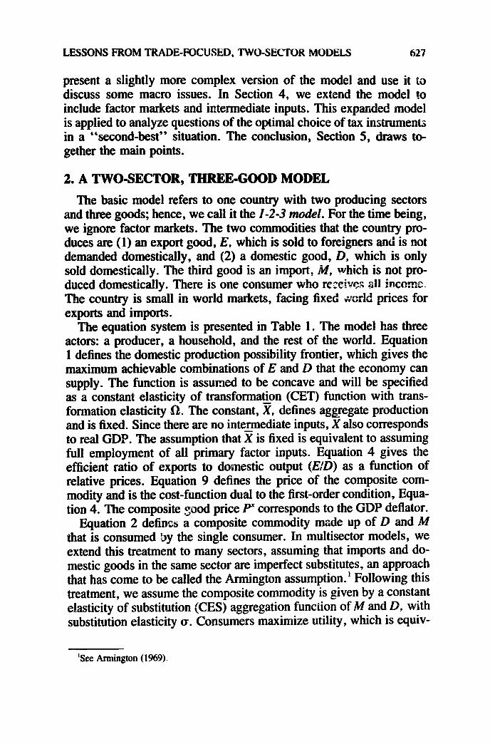
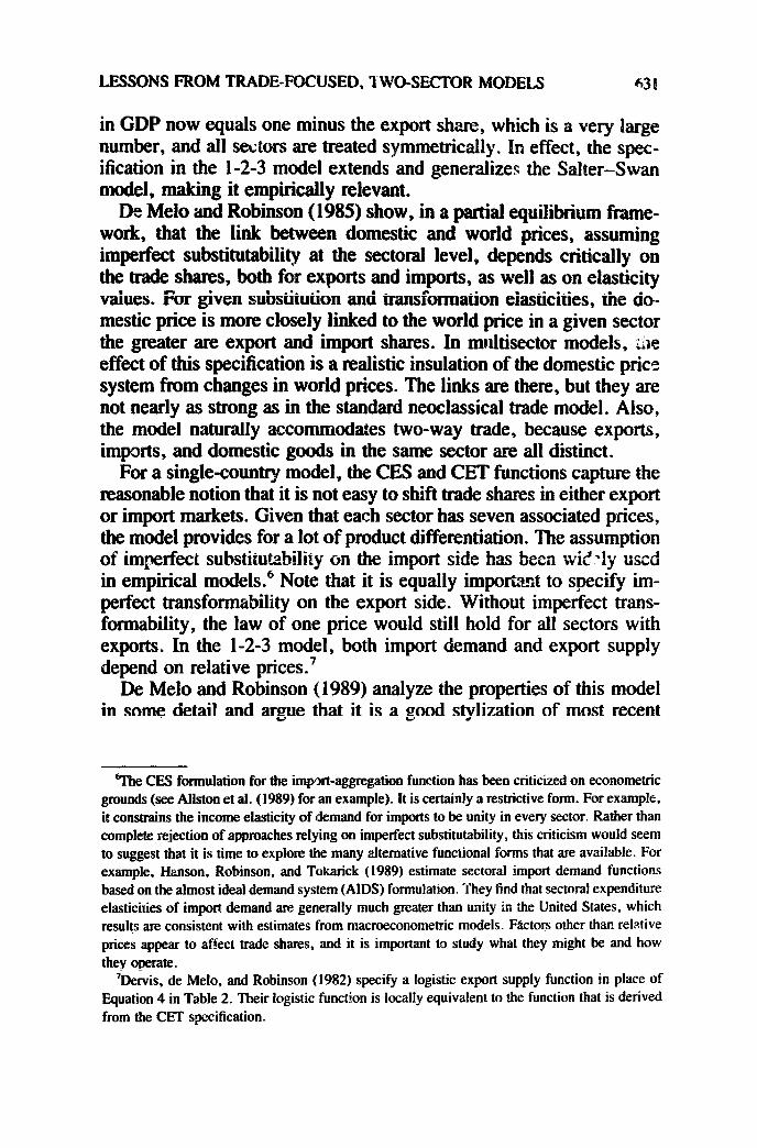
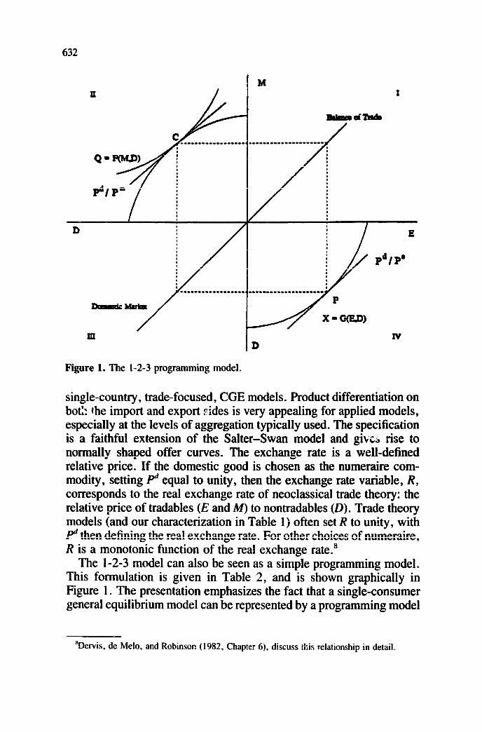
Figure 1. The l-2-3 programming model.

single-country, trade-focused, CGE models. Product differentiation on hot> she import and export sides is very appealing for applied models, especially at the levels of aggregation typically used. The specification is a faithful extension of the Salter-Swan model and give& rise to normally shaped offer curves. The exchange rate is a well-defined relative price. If the domestic good is chosen as the numeraire commodity, setting P’ equal to unity, then the exchange rate variable, R, corresponds to the real exchange rate of neoclassical trade theory: the relative price of tradables (E and M) to nontradables (0). Trade theory models (and our characterization in Table 1) often set R to unity, with pd then defining the real exchange rate. For other choices of numeraire, R is a monotonic function of the real exchange rate.8

The I-2-3 model can also be seen as a simple programming model. This formulation is given in Table 2, and is shown graphically in Figure 1. The presentation emphasizes the fact that a single-consumer general equilibrium model can be represented by a programming model

*Dervis, de Melo, and Robinson (1982, Chapter 6), discuss this relationship in detail.

LESSONS FROM TRADE-FXXJSED, TWO-SECTOR MODELS 633

that maximizes consumer utility, which is equivalent to social welfare.g In this model, the shadow prices of the constraint equations correspond to market prices in the CGE model. lo We will use the graphical ap- paratus to analyze the impact of two shocks: an increase in foreign capital inflow and a change in the international terms of trade. I’ We will also use this programming-model fommlation, including endogenous prices and tax instruments, to derive optimal policy rules under second-best conditions.

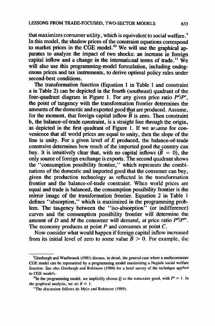
The transformation function (Equation 1 in Table 1 and constraint a in Table 2) can be depicted in the fourth (southeast) quadrant of the four-quadrant diagram in Figure 1. For any given price ratio PIP’, the point of tangency with the transformation frontier determines the amounts of the domestic and exported good that are produced. Assume, for the moment, that foreign capital inflow B is zero. Then constraint b, the balance-of-trade constraint, is a straight line through the origin, as depicted in the first quadrant of Figure 1. If we assume for con- venience that all world prices are equal to unity, then the slope of the line is unity. For a given level of E produced, the balance-of-trade constraint determines how much of the imported good the_country can buy. It is intuitively clear that, with no capital inflows (B = 0), the only source of foreign exchange is exports. The second quadrant shows the “consumption possibility frontier,” which represents the combinations of the domestic and imported good that the consumer can buy, given the production technology as reflected in the transformation frontier and the balance-of-trade constraint. When world prices are equal and trade is balanced, the consumption possibility frontier is the mirror image of the transformation frontier. Equation 2 in Table 1 defines “absorption,” which is maximized in the programming problem. The tangency between the “iso-absorption” (or indifference) curves and the consumption possibility frontier will determine the amount of D and M the consumer will demand, at price ratio PIP”. The economy produces at point P and consumes at point C.

Now consider what would happen if foreign capital inflow increased from its initial level of zero to some value B > 0. For example, the

9Ginsburgh and Waelbroeck (198 I) discuss, in detail, the general case where a multiconsumer CGE model can be represented by a programming model maximizing a Negishi social welfare function. See also Ginsburgh and Robinson (1984) for a brief survey of the technique applied to CGE models.

“In the programming model, we implicitly choose Q as the numzraire good, with P” = I. In the graphical analysis, we set R = I.

“The discussion follows de Melo and Robinson (1989).

634

Figure 2. Increase in foreign capital inflow,

country gains additional access to world capital markets or receives some foreign aid. Alternatively, there is primary resource boom in a country where the resource is effectively an enclave, so that the only direct effect is the repcitriation of export earnings. ‘* In all of these cases, we would expect domestic prices to rise relative to world prices and the tradable sector to contract relative to the nontradable sector. In short, the country would contract “Dutch disease.”

That this is indeed the case can be seen by examining Figure 2. The direct effect is to shift the balance of trade line up by B. This shift, in turn, wiJ1 shift the consumption possibility frontier up vertically by the Lame B. The new equilibrium point will depend on the nature of the erryori aggregation function (the consumer’s utility function). In Figure 2, the consumption point moves from C to C*, with increased demand tar both D and M and an increase in the price of the domestic good, P’. On the production side, the relative price has shifted in favor of the domestic good and against the export-an appreciation of the real exchange rate.

“See Benjamin and Devarajan ( 1985) or Benjamin, Devarajan, and Weiner ( 1989).

LESSON FROM TRADE-FOCUSED, TWO-SECTOR MODELS 635

Will the real exchange rate always appreciate? Consider two polar extremes, which bracket the range of possible equilibria. Suppose the elasticity of substitution between imports and domestic goods is nearly infinite, so that the indifference curves are almost flat. In this case, the new equilibrium will lie directly above the initial one (point C), since the two consumption possibility curves are vertically parallel. The amount of V consumed will not change and all the extra foreign exchange will go towards purchasing imports. By contrast, suppose the elasticity of substitution between M and D is zero, so the indifference curves are L-shape% In this case (assuming homotheticity of the utility function), the new equilibrium will lie on a ray radiating from the origin and going through the initial equilibrium. In this new equilibrium, there is more of both V and M consumed, and the price ratio has risen. Since P” is fixed by hypothesis, pd must have increased-a real appreciation. The two cases bound the range of possible outcomes. The real exchange rate will appreciate or, in the extreme case, stay unchanged. Production of D will either remain constant or rise and production of E, the tradable good in this economy, will either stay constant or decline. The range of intermediate possibilities describes the standard view of the Dutch disease.

Consider now an adverse terms-of-trade shock represented by an increase in the world price of the imported good. The results are shown in Figure 3. The direct effect is to move the balance of trade line, although this time it is a clockwise rotation rather than a trans- lation (we assume that initially B = 0). For the same amount of exports, the country can now buy fewer imports. The consumption possibility frontier is also rotated inward. The new consumption point is shown at C*, with less consumption of both imports and domestic goods. On the production side, the new equilibrium is P*. Exports have increased in order to generate foreign exchange to pay for more expensive imports, and P’Ipd has also increased to attract resources away from D and into E. There has been a real depreciation of the exchange rate.

Will there always be a real depreciation when there is an adverse shock in the international terms of trade? Not necessarily. The char- acteristics of the new equilibrium depend crucially on the value of u, the elasticity of substitution between imports and domestic goods in the import aggregation function.

Consider the extremes of u = 0 and o= = m. In the first case, as in Figure 3, there will be a reduction i:i the amount of domestic good produced (and consumed) and a depreciation of the real exchange rate. In the second case, however, flat indifference curves will have to be

636

Figure 3. Change in world prices.

tangent to the new consumption possibility frontier to the left of the old consumption point (C), because the rotation flattened the curve. At the new point, output of D rises and the real exchange rate appre- ciates. When o = 1, there is no change in either the real exchange rate or the production structure of the economy. The intuition behind this somewhat unusual result is as follows.‘3 When the price of imports rises in an economy, there are two effects: an income effect (as the consumer’s real income is now lower) and a substitution effect (as domestic goods now become more attractive). The resulting equilibrium will depend on which effect dominates. When o < 1, the income effect dominates. The economy contracts output of the domestic good and expands that of the export commodity. In order to pay for the needed, nonsubstitutable import, the real exchange rate depreciates. However, when u > 1, the substitution effect dominates. The response of the economy is to contract exports (and hence also imports) and produce more of the domestic substitute.

13We derive the result analytically below.


For most developing countries, it is likely that u < 1, so that the standard policy advice to depreciate the real exchange rate in the wake of an adverse terms-of-trade shock is correct. For developed economies, one might well expect substitution elasticities to be high. In this case, the response to a terms-of-trade shock is a real revaluation, substitution of domestic goods for the more expensive (and noncritical) import, and a contraction in the aggregate volume of trade. In all countries, one would expect substitution elasticities to be higher in the long run. The long-run effect of the real exchange rate will thus differ, and may be of opposite sign, from the short-run effect.

The relationship between the response of the economy to the terms- of-trade shock and the elasticity of substitution can also be seen by solving the model algebraically. By considering only small changes to the initial equilibrium, we can linearize the model and obtain ap- proximate analytical solutions. We follow this procedure to analyze the impact of a terms-of-trade shock.14

Let a (“*“) above a variable denote its log-differential. That is, 2 = d(lnz) = dzlz. Log-differentiate Equations 4, 5, and 14 in Table 1, assuming an exogenous change in the world price of the import. The results are:

ti-b = u (P - Pw”);

Eliminating a, D, and & and solving for @” gives

Thus, whether P’ increases or decreases in response to a terms-of- trade shock depeitds on the sign of (a - l), confirming the graphical analysis discussed above. Note that the direction of change in pd will determine how the rest of the economy will adjust in this counterfactual experiment. If pd falls (the real exchange rate depreciates), exports will rise and production of the domestic good will fall.

Our analysis with the l-2-3 model has yieldt;J several lessons.

14De Melo and Robinson (1989) derive the closed-form solution for the country’s offer curve in the l-2-3 model. A more complete discussion and mathematical derivation is given in De- varajan, Lewis, and Robinson (1990).


First, the bare bones of multisector general equilibrium models are contained in this small model. Second, and perhaps more surpris- ingly, this two-sector model is able to shed light on some issues of direct concern to developing countries. For Lxample, the appreciation of the real exchange rate from a foreign capital inflow,. widely understood intuitively and derived from more complex models, can be portrayed in this simple model. In addition, results from this small model challenge a standard policy dictum: Always depreciate the real exchange rate when there is an adverse terms-of-trade shock. The model shows the conditions under which this policy advice should and should not be followed.

Of course, many aspects of the economy are left out of the small model. In particular, there is no government. If a model is to be useful for policy analysis, it should contain the relevant policy instruments and actors. In the next section, we extend the l-2-3 model to include them.

3. THE P-2-3 MODEL WITH GOVERNMENT AND INVESTMENT

Up to now, the focus has been on adjustments in the real exchange rate in response to exogenous shocks to the economy. Dowever, the real exchange rate is not an instrument that the government directly controls. Rather, most governments use taxes and subsidies as well as expenditure policy to adjust their economies. The model presented in the previous section did not explicitly incorporate these fiscal instruments. Nor did it include important components that would allow consideration of macroeconomic issues such as the relationships among macro aggregates. Table 3 presents an extended version of the l-2-3 model to include government revenue and expenditure and also savings and investment. Three price-wedge government policy instruments are included: an import tariff, an export subsidy, and an indirect tax on domestic sales. In addition, savings and investment are included. The single household saves a fraction of its income. Real government expenditure is assumed fixed and the government deficit or surplus is subtracted or added to aggregate savings. Finally, the balance of trade is assumed to represent foreign savings.

3A. T el ln a Social Accounting Matrix

Equations 6 to 9 in Table 3 determine the income flows in the economy. The model has four actors: a producer, a household, gov- emn.;nt, and the rest of the world. Equation 6 determines government


Table 3: The l-2-3 Model with Government and Investment

Real Blows Prices (1) x = G(E,D%) (10) P’” = (1 + t”) - R . pw’”

(210’ = F(MD%) (3) e” = C/P + z + 5

(Il)pc = (1 + f)-R*pw’ (12)P = (1 + typ”

(4) ElDY = gAw-9 (13) p” = g,~~,pd) (5) M1L.P = fdp”,p? (14) p = f,(p”,p3

Nominal Flows (15) R = 1

(6)T= t”.R.pw”*M Equilibrium Conditions +f*P*DD (16) @ l 0” = 0 -P-R.pk*E (17) e” - e” = 0

(7) Y = P * 3 (18)~~“‘. M - pw’ * E = ii (8) S = &Y+R.B+F (19) p4 * z - s = 0 (9) c = Y-S-Y (20) T * P” . ?i - S* = 0

Accounting Identities (i)P*z=P.E + P“.o”

Endogenous Variables E: Export good M: Import good D’: Supply of domestic good DD: Demand for domestic good @ Sq$y of composite good Q”: Demand for composite good P: Domestic pries of export good p”: Domestic price cf import good p’: Producer price of tiomestic good P: Consumer price of dotzestic good P: Price of aggregate output P? Price of composite good R: Exchange rate T: Net government revenue

Sg: Government savings Y: Total income

C: Aggregate consumpt’i>n S: Aggregate savings Z: Aggregate real investment

Exogenous Variables pw”: World price of import good pw’: World price of export good

z“‘: Tariff rate I’: Export subsidy rate P: Indirect tax rate s: Average savings rate

z: Aggregate output z: Real goverrment demand E: Balance of trade 51: Export transformation elasticity u: Import substitution elasticity

revenue (net of export subsidies) and Equation 7 determines household income. Equations 8 and 9 determine total savings and aggregate household consumption. The nominal flows among the actors can be tabulated in a social accounting matrix (SAM), which is presented in Figure

640 S. Devarajan, 5. D. Lewis, and S. Robinson

4. I5 The SAM shows the circular flow of income and expenditure in the economy. Each ccl represents a payment from a column account to a recipient in a ro ccount. The SAM is square and, following the conventions o ntry bookkeeping, each actor’s accounts must balance: Income st exactly equai expenditure. Thus, column sums in the SAM m al the corresponding row sums.

s six accounts, one for each actor, one for savings and investment, nd an additional * ‘commodity” account. The

track of absorption, which equals the value on the domestic market, D, and imports, pays out total revenue to households and

umn and sells goods on the domestic and . The column sum equals GDP at market

prices, which includes indirect taxes. GDP at factor cost equals F l X and is paid out to households. Export subsidies are seen as a payment by government to producers. Exports and imports in the account for the rest of the world are valued in world market prices times the exchange rate.

The capital account in the SAM reflects savings-investment balance. It summarizes the workings of the financial system, representing the net loanable funds market. It collects savings along the row and spends them on investment goods in the column. The allocation of new capital goods by sector of destination is not shown. The model thus captures the savings-investment nexus in a stylized manner and also includes other macro aggregates. As we show below 9 it can provide a framework for some macro analysis.

. Macro Closure

The macroeconomic properties of CGE models of developing countries have provided a t pit for much debate and controversy. The discussion has focused on what has come to be called the “macro closure” of an ide model? As the SAM indicates, the extended l-2-3 ins the three basic macro balances: balance of trade, savin t, and government deficit. l[n this model, the balance of trade is fixed and real government expenditure is fixed. The government deficit is determined residually as expenditure minus

lSPyatt and Round (1985) provide a good introduction to SAMs and a number of examples of their uses.

‘%e seminal work on closure is Sen ( 1963). The development literature is surveyed by Rattso (1982) and by Robinson (1989a,b).

Rec

eipt

s

Com

mod

ity

Prod

ucer

Hou

seho

ld

Gov

ernm

ent

Cap

ital

acco

unt

Res

t of

wor

ld

Tot

al

Exp

endi

ture

s

Com

mod

ity

Pro

duce

r H

ouse

hold

G

over

nmen

t C

apit

al

Wor

ld

I

p-e

s G

DP

+

T’

Def

init

ions

:

M=R-~W-M

T'=f-pd'Dd

E=~-phf-E

l-=P-R-pw'-E

T"=f.R-pw".M

GD

P

=

F’

- 2

=

GD

P a

t fa

ctor

cos

t

P.?

+.Id

-T+T

”=C

+p9+

G+p

-Z+E

-&=G

DP

atm

arke

tpri

ces

All

othe

r va

riab

les

are

defi

ned

in T

able

3.

re 4

: So

cial

Acc

ount

ing

Mat

rix

for

l-2-

3 M

odel

with

Gov

ernm

ent

and

3nve

slm

ent


net tax receipts. Aggregate savings is the sum of household saving, government saving (surplus), and the balance of trade (foreign saving). There is no separate investment function, so aggregate investment is simply equal to aggregate savings. This savings-driven investment determination represents a macro specification that is called “neoclassical closure. * ’

In addition, the m-ode1 implicitly assumes full employment, so aggregate real GDP (X in Equation 1) is fixed. While all the macro balances are in the model, there is little room for any interesting macro behavior. There is no possible feedback from changes in macro aggregates to GDP and little scope for variation in the macro aggregates themselves. Given the assumed savings behavior, no special equilibrating variable is required to achieve savings-investment equilibrium. The model is specified in terms only of current flows and flow- equilibrium conditions. There are no assets, no asset markets, no money, no expectations, and no dynamics.

The extended l-2-3 model represents a Walrasian CGE model. While it contains macro aggregates, as must any economywide model, it is best seen as a neoclassical general equilibrium mod4 of production and exchange. The additions of government, savings-investment, and the balance of trade are done in ways that retain the notion of flow equilibria and do not strain the Walrasian paradigm. However, as the development literature illustrates, it is possible to bring in a lot of macro effects while remaining within the framework of a CGE model that includes only flow variables.

The literature on macro closure has followed two different approaches to bringing macro features into the model. In the first approach, relationships are specified among the macro aggregates, but their justification is based on macroeconomic theory outside of the CGE model. At one extreme, all the macro variables are specified as exogenous to the model.” In a second approach, the CGE model is extended to include variables typically found in macro models (such as money, assets, and interest rates) and to expand the notion of equilibrium to incorporate asset markets and expectations. The intent is to build CGE models that move beyond the Walrasian paradigm and directly incorporate macro phenomena. ‘*

In the first approach, in effect, the CGE model is forced to interact

“Or almost all. The CGE model still must satisfy Wah-ac’s Law and the various quilibrium conditions are not all independent. For an example of a CGE model which draws on a separate macro model to determine the macro aggregates, see Hanson, Robinson, and Tokarick (1989).

%ewatripont and Miche! (1987) argue for this approach.

LESSON FROM TRADE-F SEX TWO-S ODELS 3

with a macro model, bu 0 models are kept as separate ev-a be fully spelled out.

8 of developing countries and in a few

ided by Devarajan and de Melo (1987), who discuss a CGE m 1 applicable to franc zone African countries. In these countries, the al currency is tied to the French franc, so they have no independent monetary authority. In addition, it is reasonable to assume th vemment expenditure and aggregate investment are fixed exoge . Given fixed tax rates, government revenue and private savings t suffice to finance government expenditure and aggregate investment. Any shortfall is financed by foreign borrowing. In effect, for these countries the French Central Bank finances the sum of the twin deficits.”

The extended l-2-3 model can easilyy be adapted to incorporate these assumptions. In Table 3, fix aggregate real investment as well as real government expenditure. The model is now investment-driven rather than savings-driven. To achieve savings-investment equilibrium, the balance of trade is now treated as an endogenous variable. It is the macro equilibrating variable that will vary to equate savings (the sum of private, government, and foreign savings) and investment. The nominal exchange rate is chosen as numeraire, reflecting the fact that the exchange rate in these countries is tied to the French franc. The domestic price level will vary to produce a real exchange rate that generates a balance of trade that achieves macro balance. The CGE model will thus solve for a flow equilibrium that is consistent with the assumed macro behavior. The model incorporates macro rigidities, in particular the government revenue constraint. If government revenue changes, say by changing taxes, the effect will be to change the balance of trade because the government deficit is financed by foreign borrowing.

19See Powell (I 98 I), who describes how the Orani model of Australia was linked to a separate small macro model. Robinson and Tyson (1984) formally describe the notion of linking macro and @GE models and relate the idea to the literatme on macro closure. Many of the structural adjustment models of developing countries that trace their roots to Dervis, de Melo, and Robinson (1982) are in this tradition.

%uch a view may seem extreme. However, consider recent U.S. history. While the macro story is more complex, the net result is essentially the same. The United States has financed the federal deficit by foreign borrowing, the Japanese playing the role of the French Central Bank.

644 S. Devarajan, J. D. Lewis, and S. Robinsm

Given the focus on the government budget, the model can be further simplified by setting aggregate real investment to zero. Devarajan and de &I& assume that real government demand for the domestic good is fixed and add the balance of trade directly to government revenue. The macro equilibrating mechanism is unchanged, with the government deficit directly linked to the balance of trade.

Unfortunately, even with these simplifying assumptions, this model does not lend itself to the same four-quadrant, diagrammatic analysis used above. Given the assumption that the current account is determined endogenously, any change in consumption or production that changes government revenue will also change the balance of trade (shifting the balance of trade constraint line in Figure 1). Any shock will likely have a compound effect, shifting curves in more than one quadrant.21 The model, however, does yield analytic results anaIogous to those from the l-2-3 model. This model indicates that these economies might well react in ways counterintuitive to some standard policy packages.

Consider, for example, the effect of an increase in the tariff rate. The initial eflect is a rotation of the consumer’s budget line, making imports more expensive. In the l-2-3 model with a fixed balance of trade, the final result would by lower import demand, appreciation of the exchange rate, an incentive bias against exports, and lower exports. An import tariff represents a tax on exports--a proposition known as Lemer symmetry. In the Devarajan-de Melo model, however, macro feedbacks can change this result. The increase in the tariff rate increases government revenue, thus lessening foreign borrowing and improving the balance of trade. The lower balance of trade generates a real depreciation, offsetting the real appreciation associated with the tariff increase, and encouraging exports (E). Whether exports actually increase depends on u, the elasticity of substitution between the import (M) and domestic good (0). The reason is that, in this model, none of the tariff revenue is transferred to the consumer. Instead, it is used to reduce foreign borrowing. Thus, when the tariff rate is increased, the consumer faces a higher domestic price for M, with no change in income. When o > 1, the consumer buys more D and less M. However, if CT < 1, the consumer buys less of both goods. The lower consumption of D releases resmrces to the exportable sector, raising E. The coun-

“Devarajan and de Melo (1987) present an alternative diagrammatic approach for analyzing simple shocks with this model.


terintuitive result in this case is that the tariff increase leads to a rise in exports.

Finally, consider the impact of a change in the international terms of trade; for example, an increase in the world price of exports. In the l-2-3 model, with a fixed balance of trade, the new equilibrium will have an increase in absorption Q (and hence in welfare j. As discussed above, what happens to the volume of exports and imports, and to domestic relative prices, depends on the elasticity of substitution o. The increase in the price of exports generates an income effect as well as a substitution effect. Income goes up, leading to an increase in demand for both D and M. If o is less than unity, the income effect dominates and, in the final equilibrium, consumption of both domestic goods and imports (D and _V) will be higher and exports lower, and the real exchange rate will appreciate. In the Devarajan-de Melo model, however, there is a second macro income effect. Appreciation of the real exchange rate raises the price of D. An increase in pd will increase the cost of fixed government demand for D, worsening the government budget deficit, and leading to increased foreign borrowing.** The net effect is that the balance of trade deteriorates, with greater appreciation of the final equilibrium real exchange rate. Thus, with u < 1, the net effect of a beneficial increase in export prices is to worsen the balance of trade. Devarajan and de Melo cite empirical evidence that indicates that this outcome is consistent with the behavior of many franc zone African countries.

In the Devarajan-de Melo model, the macro effects are purely structural in the sense that they affect only the composition of the economy. Given the maintained assumption that factors are fully employed and that factor markets clear, the changes in macro aggregates will have little or no effect on aggregate real GDP. Many of the structural adjustment models maintain the assumption of full employment. There is, however, a strand of work with CGE models that incorporates mechanisms that permit changes in macro aggregates to generate unemployment. For example, Devarajan and de Melo specify a variant of their model with a fixed wage? thus allowing aggregate employment effects in response to shocks. These “macro structuralist” models all have in common the assumption that at least some factor and product

*mere is a countervailing effect because, as imports rise, so does tariff revenue. The effect is not large enough to offset the increase in the price of the domestic good. This result is sensitive to the assumption that government demands only the domestic good.


markets do not clear.23 They postulate various rigidities, such as sec- torally immobile capital, fixed wages, mark-up pricing, a fixed exchange rate, and/or various kinds of rationing in product and factor markets. They can generate Keynesian unemployment (or Keynesian closure) qd so postulate strong links between macro balances and the real side of the economy.

The literature on macro closure demonstrates that neoclassical CGE models that contain no assets or money can still be useful in analyzing the impact of changes in macro aggregates on the economy. However, the marriage is an uneasy one. A macro model or scenario is forced onto the CGE model, which then traces out the structural implications of the assumed macro behavior. There are no optimizing agents (either private or government) that generate the macro behavior. The macro structuralist models further strain the neoclassical paradigm because they assume that various markets do not clear and that certain agents within the model economy do not optimize.

Introducing taxes, subsidies, and government expenditure adds more than just missing instruments and macroeconomic behavior to the two- sector model. It captures a fundamental fact in public economics: It is costly to transfer resources from the private to the p;;Iblic sector. Since governments do not have access to lump-sum taxes, they must use second-best taxes, which by definition distort incentives and create efficiency losses in the economy. One goal of structural adjustment policy often expressed in World Bank and IMF reports is to reduce these distortions and improve the allocation of resources. Nevertheless, governments continue to need revenue so that eliminating all taxes is not an option. In the next section, we extend the l-2-3 model further to include factor markets and intermediate goods, and then use this model to determine optimal taxes under various second-best scenarios. As we will see, some of the policy rules of thumb do not necessarily improve the efficiency of the economy.

4. A TWO-SECTOR MODEL WITH FACTOR MARKETS INTERMEDIATE GOODS

When considering the efficiency effects of tax policy, it is critical to distinguish between intermediate and final goods. The models presented earlier do not make this distinction. In this section, we extend

ULance Taylor is a leader in this field. See Taylor (1983). Recent CGE models in this tradition with a focus on agriculture are surveyed by de Janvry and Sadoulet (1987). Adelman and Robinson (1988) compare various macro closures in two archetype models.


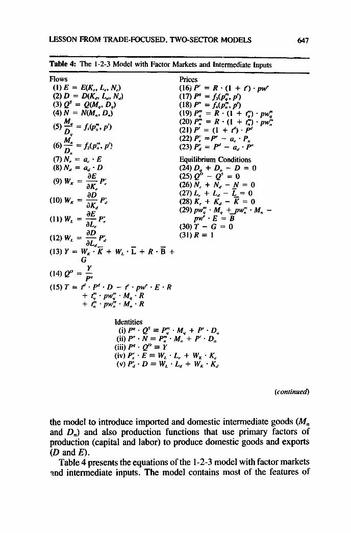
Table 4: The l-2-3 Model with Factor Markets and Intermediate Inputs

mows (1) E = EK, L NJ (2) D = DWd, Ld, Ndl (3) 0’ = QW,, 0,) (4) N = WL m

(5)2 = my, P’)

(6-)$ = h(PIr9 P? n

(7) IV, = Q, - E (8) IV‘, = a,, - D

(9) w, = g PI

(10) w, = g Pi d

(11) w, = g P:

(12) w, = g P; d-

(13) Y = w, ’ K + w, . G

Prices (16jP = I?.(1 + f).pw’ (17) p = f,(PY, j-0 (18) p” = h(pt’, p? (19) Py = R - (1 + fy, *pwr (20) Pf = R - (1 + C) - pw; (21)p’ = (1 + fyp (22) Pi =P - a, - P, (23) Pi = P” - ad - P”

Equilibrium Conditions (24) 0, + 0, - D = 0 (25) @ - e” = 0 (26) N, + Nd - ,N = 0 (27) L, + Ld - &= 0 (28) K, + & - K = 0 (29) pw:: - M, +gw; - M. -

pw’ - E = B (30) T - G = 0 (31) R = 1

I]+R.B+

(14) e” = ;

(15)T= t’.P“*D - f.pw=E.R + c - pw; - M, - R + c*pw;.M;R

Identities (i)p4.@=PT.Mq + P’.D,

(ii) P” - N = Pr - M, + P’ * D, (iii) p9 . @ = Y (iv) P,’ - E = W, * L, + W, - K, (V) P; - D = W, - Ld + w, - Kd

the model to introduce imported and domestic intermediate goods (M, and D,) and also production functions that use primary factors of production (capital and labor) to produce domestic goods and exports (D and E).

Table 4 presents the equations of the l-2-3 model with factor markets and intermediate inputs. The model contains most of the features of

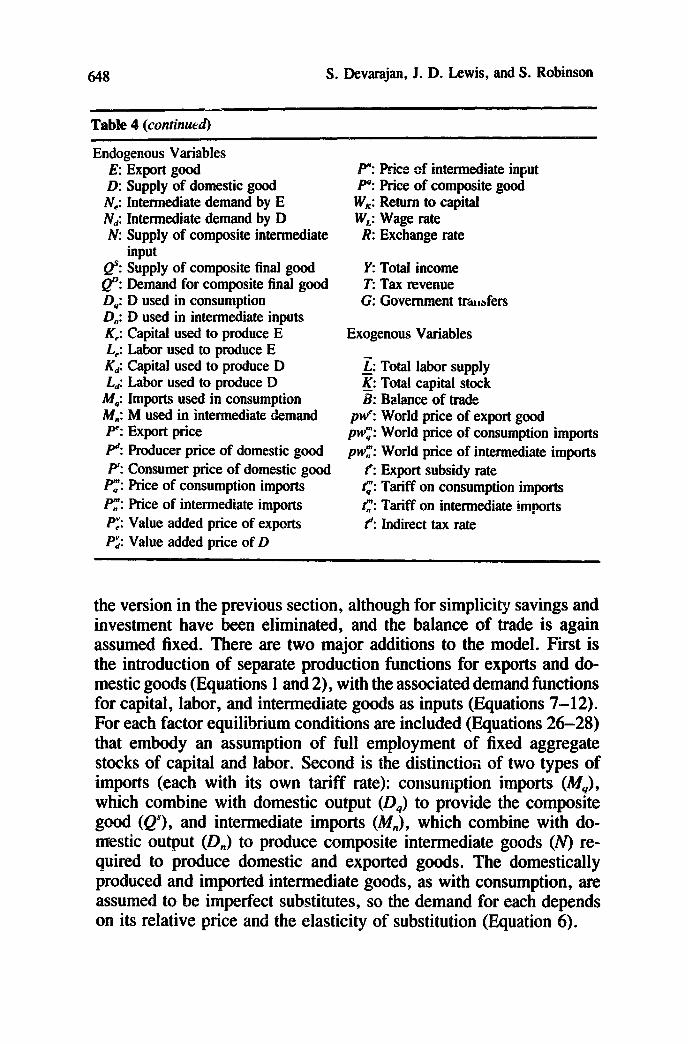
648 S. Devmjan, J. D. Lewis, and S. Robinson

Table 4 (continued)

Endogenous Variables E: Export good D: Supply of domestic good N,: Nd: N:

Intermediate demand by E Intermediate demand by D Supply of composite intermediate input

0’: fg:

4: 0,: K,: L,: K,,: L&$: M,: M,: .

:I p: y: c: PZ: Pi:

Supply of composite final good Demand for composite final good D used in consumption D used in intermediate inputs Capital used to produce E Labor used to produce E Capital used to produce D Labor used to produce D Imports used in consumption M used in intermediate demand Export price Producer price of domestic good Consumer price of domestic good Price of consumption imports Price of intermediate imports Value added price of exports Value added price of D

P? Price of intermediate input p4: Price of composite good

WK: Return to capital WL: Wage rate R: Exchange rate

Y: Total income T: Tax revenue G: Government triu,afers

Exogenous Variables

z Total labor supply 5: Total capital stock B: Bafance of trade

pw’: World price of export good pwr: World price of consumption imports pwr: World price of intermediate imports

f: Export subsidy rate c: Tariff on consumption imports c: Tariff on intermediate imports fi Indirect tax rate

the version in the previous section, although for simplicity savings and investment have been eliminated, and the balance of trade is again assumed fixed. There are two major additions to the model. First is the introduction of separate production functions for exports and domestic goods (Equations 1 and 2), with the associated demand functions for capital, labor, and intermediate goods as inputs (Equations 7-12). For each factor equilibrium conditions are included (Equations 26-28) that embody an assumption of full employment of fixed aggregate stocks of capital and labor. Second is the distinction of two types of imports (each with its own tariff rate): consumption imports (MJ, which combine with domestic output (D,) to provide the composite good (es), and intermediate imports (M,), which combine with domestic output (D,) to produce composite intermediate goods (IV) required to produce domestic and exported goods. The domestically produced and imported intermediate goods, as with consumption, are assumed to be imperfect substitutes, so the demand for each depends on its relative price and the elasticity of substitution (Equation 6).

LESSON FROM TRADE-FC?‘! JSED, TWO-SECTOR MODELS 649

value added IVI

CES

imported input

dommic

input

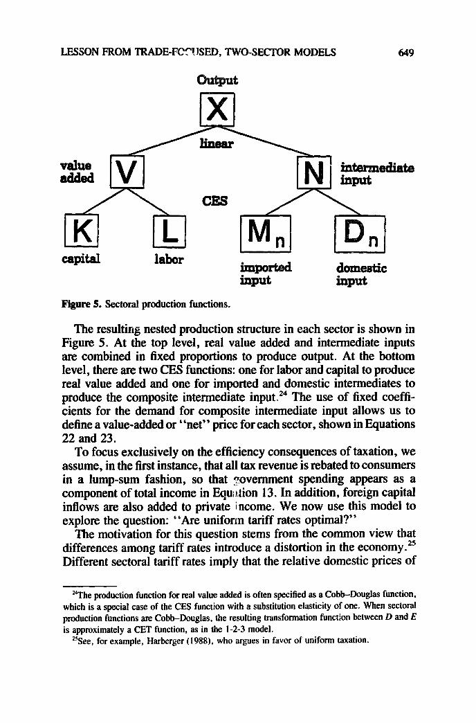
Figure 5. Sectoral production functions.

The resulting nested production structure in each sector is shown in Figure 5. At the top level, real value added and intermediate inputs are combined in fixed proportions to produce output. At the bottom level, there are two CES functions: one for labor and capital to produce real value added and one for imported and domestic intermediates to produce the composite intermediate input.24 The use of fixed coeffi- cients for the demand for composite intermediate input allows us to define a value-added or “net” price for each sector, shown in Equations 22 and 23.

To focus exclusively on the efficiency consequences of taxation, we assume, in the first instance, that all tax revenue is rebated to consumers in a lump-sum fashion, so that Tovernment spending appears as a component of total income in Equation 13. In addition, foreign capital inflows are also added to private i ‘ncome. We now use this model to explore the question: “Are uniform tariff rates optimal?”

The motivation for this question stems from the common view that differences among tariff rates introduce a distortion in the economy2’ Different sectoral tariff rates imply that the relative domestic prices of

‘4The production function for real value added is often specified as a Cobb-Douglas function, which is a special case of the CES function with a substitution elasticity of one. When sectoral production functions are Cobb-Douglas, the resulting transformation function between D and E is approximately a CET function, as in the l-2-3 model.

“See, for example, Harberger (1988), who argues in favor of uniform taxation.


Table 5: SAM for Stylized Numerical Model

Expenditures

ACtlVltleS commodltles Factors Rest of

Export Domestic Final Intermed Labor Capital Consumer world

Expfi w 30 Domestic (D) 73 2 Final good(Q) 100 Intermediate 5 (N) Labor (L) 20 30 Capital (K) 8 45 Consumer 50 50 Rest of world 27 3

Total 30 75 loo 5 50 50 loo 30

two traded goods are not equal to their relative world prices. If world prices are viewed as the appropriate “shadow prices” of these traded goods, a varied tariff structure represents a distortion. However, if there are other distorting taxes in the economy, then the shadow prices of these traded goods in this second-best environment may not equal world prices. 26 In particular, if the domestic indirect tax structure is not optimal, the optimal tariff structure will generally not be uniform. We investigate this question by determining the optimal pattern of tariffs under various assumptions about the level of domestic indirect taxes. Introducing intermediate goods complicates the model sufti- ciently so that we cannot solve the model analytically. We proceed by computing numerical solutions to our optimization problem by using stylized data.27

Table 5 presents the base data for the numerical application. Real GDP equals 100 and the model economy exports and imports 30. The export sector (E) is labor-intensive and uses domestic and imported intermediates. The domestic sector (0) uses no intermediates. The balance of trade is zero and the single consumer thus demands 100 units of the composite consumer good ((2). Since all prices and wages equal unity, the SAM indicates real as well as nominal magni- tudes. The value-added production functions are assumed to be Cobb-

Chambers (19891,

is solved a nonlinear programming package called CAMS. See Brooke, Kendrick. and Meeraus (1988).


Douglas. The elasticity of substitution between imports and domestic goods (0) is equal to 2 for consumer goods and 0.5 for intermediate goods.

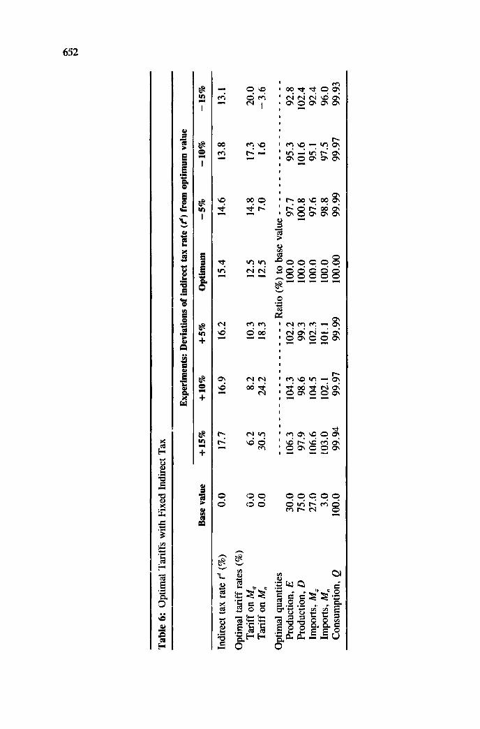
In the experiments, the government raises revenue with three tax instruments: tariffs on final and intermediate goods and an indirect tax on domestic sales. There is no export subsidy. The government is assumed to require total tax revenue of 15. The base data given in Table 5 represent a unique solution of the model with all tax rates set to zero. In the optimal tax experiments, choice is introduced by re- defining the tax rates as variables. Optimal taxes are determined by maximizing Q subject to the equations of the CGE model plus the government revenue constraint. Alternative second-best scenarios are considered by also fixing one tax, the indirect tax on domestic goods (p>, and solving for optimal levels of tariff rates (the only remaining tax instruments).

The results are given in Table 6. The optimal pattern of tariffs is uniform only in the special case when the indirect tax is also set optimally.z8 When the indirect tax is below its optimal value, the second-best optimal tariff structure is to have a higher tariff on the final good than on the intermediate good. When the indirect tax is set at a level 15 percent below its optimum value, the best policy is to subsidize intermediate imports. The reverse is true when the indirect tax is above the optimum. In this case, the second-best optimum in- volves higher tariffs on imported final goods than on imported intermediates. In general, one would expect that domestic indirect taxes are too low rather than too high in developing countries. Thus, the appropriate policy rule of thumb is that tariff rates on intermediates should be lower than the rates for consumer goods.

Given the mistaken view that equal tariffs are best, it is often sug- gested that countries should at least move toward equal rates by raising the lowest tariffs and lowering the highest ones. In most developing countries, tariffs on intermediate goods are lower than those on final goods, which is consistent with our (second-best) rule of thumb. In this environment, moving toward equal rates would lower welfare.

Along with a highly variegated tariff structure9 the second-best scenarios show smaller but significant variations in real lariables. HOW-

ever, aggregate welfare varies little across the experiments. This result is consistent with results from a large number of empirical studies. Aggregate welfare gains from reducing price-wedge trade distortions

- % Table 2, the optimum indirect tax rate was determined by maximizing absovtion &?I

with all taxes, including td, as policy instruments. In the other experiments, f was fixed.

Tab

le

6:

Opt

imal

T

arif

fs

with

Fix

ed I

ndir

ect

Tax

Exp

erim

ents

: D

evia

tion

s of

ind

irec

t ta

x ra

te (

8) f

rom

opt

imum

va

lue

Bas

e va

lue

+ 1

5%

+ 1

0%

+5%

O

ptim

um

-5%

-

10%

-

15%

Indi

rect

ta

x ra

te t

” (%

)

Opt

imal

ta

riff

hat

es (

%)

Tar

iff

on M

q T

arif

f on

M,

Opt

imal

qu

antit

ies

Prod

uctio

n,

E

Prod

uctio

n,

D

Impo

rts,

M,

Impo

rts,

M

, C

onsu

mpt

ion,

Q

0.0

G.0

0.

0

30.0

75

.0

27.0

3.

0 10

0.0

17.7

16

.9

16.2

15

.4

14.6

13

.8

13.1

6.2

8.2

10.3

12

.5

14.8

17

.3

20.0

30

.5

24.2

18

.3

12.5

7.

0 1.

6 -3

.6

__-_

__--

____

____

____

R

atio

(%

) to

bas

e va

lue

- -

- -

- -

- -

- -

- -

- -

- -

- -

- -

106.

3 10

4.3

102.

2 10

0.0

97.7

95

.3

92.8

97

.9

98.6

99

.3

100.

0 10

0.8

101.

6 10

2.4

106.

6 10

4.5

102.

3 10

0.0

97.6

95

.1

92.4

10

3.0

102.

1 10

1.1

100.

0 98

.8

97.5

96

.0

99.9

4 99

.97

99.9

9 10

0.00

99

.99

99.9

7 99

.93


tend to be small.29 Substitution possibilities in production, consumption, and trade endow the economy with a great deal of adjustment flexibility. When markets work and factors are fully employed, even large price-wedge distortions cihn be vitiated by substitution possibilities, with little effect on aggregate welfare.

Two points should be noted about this result. While aggregate welfare effects may be small, the impact of policy changes on the sectoral structure of resource allocation, production, and trade tend to be more significant. In general, political pressure groups are organized by sector and care about the impact of policy on the relative position of their sector in the economy. Policymakers are more interested in measures of the structural impact of policies than in measures of aggregate welfare. Any positive analysis of policy needs to take this concern into account.

Second, while aggregate welfare losses arising from, say, distorting taxes may be small compared to aggregate GDP, they may be large relative to the tax revenue generated. Studies with CGE models indicate that a “project” that raises the same amount of tax revenue by using more efficient taxes may have a social rate of return of 20-50 percent, where the denominator is aggregate tax revenue. A similar analysis can be done with our model.

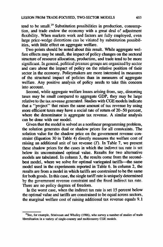
Given that the model is solved as a nonlinear programming problem, the solution generates dual or shadow prices for all constraints. The solution value for the shadow price on the government revenue constraint (Equation 30 in Table 4) directly measures the welfare cost of raising an additional unit of tax revenue (7’). In Table 7, we present these shadow prices for the cases in which the indirect tax rate is set below its unconstrained optimal value. Results for two alternative models are tabulated. In column 3, the results come from the second- best model, where we solve for optimal variegated tariffs-the same model used in the experiments reported in Table 6. In column 2, the results are from a model in which tariffs are constrained to be the same for both goods. In this case, the single tariff rate is uniquely determined by the government revenue constraint and the fixed indirect tax rate. There are no policy degrees of freedom.

In the worst case, when the indirect tax rate is set 15 percent below the optimal value and tariffs are constrained to be equal across sectors, the marginal welfare cost of raising additional tax revenue equals 9.1

?3ee, for example, Srinivasan and Whalley (1986). who survey a number of studies of trade liberalization in a variety of single-country and multicountry CGE models.


Table 7: Welfare Cost of Increasing Tax Revenue

Marginal we&re cast of increasing tax revenue as a % of additional revenue

Indirect tax rate (9%)

Constrained: equal tariffs

Second-besk diRereMial

Ratio (96) of 4zimmhedti

seamd-best

15.4 (optimal) 0.0 0.0 14.6 ( - 5%) 2.6 2.1 123.8 13.8 (- 10%) 5.6 4.3 130.2 13.1 (- 15%) 9.1 6.8 133.8

percent of the increased revenue. While smaller than rates of dead- weight loss found in the public finance literature, the loss is significant .30 If policymakers mistakenly insist that tariff rates should be equal across sectors, they will design a tax system with a marginal efficiency cost a third higher than if they use optimal variegated tariffs.

Given the stylized nature of the model, these results are only sugges- tive. Nevertheless, they do point to the frail theoretical underpinning for the common policy rule of thumb that countries should unify their tariff structure. Furthermore, they show how a small model can capture the salient aspects of this important question and guide our intuition as we investigate it with more complex models. In fact, this particular issue has been investigated with larger applied models and the results from the two-sector model appear robust.3’

This article shows how two-sector models can be used to derive policy lessons about adjustment in developing countries. Starting from a small, one-country, two-sector, three-good (l-2-3) model, we have shown how the effects of a foreign capital inflow and terms of trade shock can be analyzed. In particular, we derived the assumptions underlying the conventional policy recommendation of exchange rate depreciation in response to adverse shocks.

We next expanded the model to include savings, investment, and a

%r?e reason for t’:e relatively small marginal welfare cost is that this mtiel allows lump- sum transfers to households (Equation 13), so the only efficiexy loss comes from the price wedge.

“See Dahl, Devarajan, and van Wijnbergen (1986) and Devarajan and Lewis (1989).

LESSON FROM TRADE-FOCUSED, TWO-SEmR 6x5

range of government policy instruments, including import tariffs, export subsidies, and indirect taxes. The introduction of government, savings, and investment raises issues of macro closure. We discussed how the impact of policy interventions and exogenous shocks is sensitive to assumptions about how macro balance is achieved. We next extended the model to include factor markets and intermediate inputs. We used this extended model to explore issues of optimal tax policy. In particular, we asked whether uniform secto.ral tariff rates, a common policy prescription for improving efficiency, are optimal. We showed that equating sectoral tariff rates is optimal only when other taxes are also set optimally. In second-best environments, a better rule of thumb would be to have a high tariff rate on consumer goods and a low rate on intermediates.

The models we have presented represent a stylized picture of how developing economies function. They are useful for qualitative analysis. However, policymakers are also concerned with the magnitude of the response to their initiatives. Furthermore, they require models that incorporate the more distinctive structural and institutional features of their economies. The lessons drawn from these models facilitate the interpretation of results from more complex applied models, because they are essentially multisectoral analogues of the small models developed here.

REFERENCES

Adelman, I., and Robinson, S (1988) Macroeconomic Adjustment and Income Distribution: Alternative Models App;?ed to Two Economies, Journal of Development Economics 29: l-22.

Allston, J. M., Carter, C. A., Green, R., and Pick, D. ( 1989) Whither Armington Trade Models. American .fOlUM/ of Agricultural Economics, forthcoming.

Armington, P. (1969) A Theory of Demand for Products Distinguished by Place of Production. IMF StaflPapers 16: 159-176.

Benjamin, N., and Devarajan, S. ( 1985) Oil Revenues and the Cameroon Economy. In The Political EconomyofCameroon(1. W.ZartmanandM.Schatzberg.Eds.).NewYork:PraegerPress.

Benjamin, N., Devarajan, S., and Weiner, R. (1989) The “Dutch Disease” in a Developing Country: Oil Reserves in Cameroon. Journai of Development Economics 30 (1, January); 71-92.

Brooke, A., Kendrick, D., and Meeraus, A. (1988) CAMS: A User’s Guide. Redwood, CA: Scientific Press.

Chambers, R. G. (1989) Tariff Reform and the Uniform Tariff. Preliminary draft, May. Dahl, H., Devarajan, S., and van Wijnbergen, S. (1986) Revenue-Neutral Tariff Reform: Theory

and an Application to Cameroon. Discussion Paper No. 1986-25, Country Policy De- partment. The World Bank, May.

de Janvry, A., and Sadoulet, E. (1987) Agricultural Price Policy in General Equilibrium Models: Results and Comparisons. American Journal of Agricultural Economics 69(2, May): 230- 246.


Dervis, K., de Melo, J., and Robinson, S. (1982) General Equilibrium Models fGr Development Policy. Cambridge: Cambridge University Press.

Devmjm, S., and Lewis, J. D. (1989) Structural Adjustment and Economic Reform in Indonesia: Model-Based Policies versus Rules of Thumb. HIID Development Discussion Paper, Harvard University.

bvmjm, S., Lewis, J. D., and Robinson, S. (1990) External Shocks and the Real Exchange Rate. Depattment of Agricultural and Resource Economics, University of California, Berkeley, pmcessed.

Devmjan, S., and de Melo, J. (1987) Adjustment with a Fixed Exchange Rate: Cameroon, C&e d’Ivoire, and Senegal. world Bank Economic Review l(3): 447-487.

Dewatripont, M., and Michel, G. (1987) On Closure Rules, Homogeneity, and Dynamics in Ap- plied General Equilibrium Models. Journal of Development Economics 26( 1, June): 65-76.

Ginsburgh, V., and Robinson, R. (1984) Equilibrium and Prices in Multisector Models. In Economic Structure and Pe$ormance (M. Syquin, L. Taylor, and L. Westphal, F~s.), CIew York: Academic Press.

Ginsburgh, V., and Waelbtoeck, J. (198 1) Activity Analysis and General Equilibrium Modelling. Amsterdam: North-Holland.

Hanson, K., Robinson, S., and Tokarlck, S. (1989) United States Adjustment in the 1990’s: A CGE Analysis of Alternative Trade Strategies. Working Paper No. 510, Department of Agricultural and Resource Economics, University of California, Berkeley.

Harberger, A. (1988) Reflections on Uniform Taxation. Paper presented at the 44th Congress of the International Institute of Public Finance, Istanbul, August.

Heady, C. J., and Mitra, P. K. (1987) Distributional and Resource Raising Arguments for Tariffs. Journal of Development Economics 20: 77-101.

Melo, J. de, and Robinson, S. (1985) Product Differentiation and Trade Dependence of the Domestic Price System in Computable General Equilibrium Trade Models. In Interna- tional Trade andExchange Rates in the Late Eighties (T. Peeters, P. Praet, and P. Reding, Eds.). Amsterdam: North-Holland.

Melo, J. de, and Robinson, S. (1989) Product Differentiation and the Treatment of Foreign Trade in Computable General Equilibrium Models of Small Economies. Journal of fn- ternational Economics 27: 47-67.

Powell, A. A. (1981) The Major Streams of Economy-wide Modelling: Is Rapprochement Pos- sible?” In Large-Scale Macroeconometric Models (J. Kmenta and J. B. Ramsey, Eds.). Amsterdam: North-Holland.

Pyan, G. and Round, J. T., Eds. (1985) Social Accounting Matrices: A Basis for Planning. Washington, DC: World Bank.

Ranso, J. (1982) Different Macroclosures of the Original Johansen Model and Their Impact on Policy Evaluation. Journal of Policy Modeling 4( 1): 85-97.

Robinson, S. (1989a) Computable General Equilibrium Models of Developing Countries: Stmtch- ing the Neoclassical Paradigm. Working Paper No. 513, Department of Agricultural and Resource Economics, University of California, Berkeley.

Robinson, S. (1989b) Multisectoral Modeis. in Handbook of Deveiopment Economics (H. B. Chenery and T. N. Srinivasan, Eds.). Amsterdam: North-Holland.

Robinson, S. and Tyson, L. D. (1984) Modelling Structural Adjustment: Micro and Macro Elements in a General Equilibrium Framework. In Applied General Equilibrium Analysis (H. Scarf and J. B. Shoven, Eds.). Cambridge: Cambridge University Press.

Salter, W. (1959) Internal and External Balance: The Role of Price and Expenditure Effects. Economic Record 35: 226-238.

Sen, A. K. (1963) Neo-Classical and Neo-Keynesian Theories of Distribution. Economic Record 39: 53-66.


Stinivasan, T. N., and Whalley, J., Eds. (1986) General Equilibrium Trade P&y Modeling. Cambridge, MA: MIT Press.

Swan, T. (1960) Economic Controi ia, a Dependent Economy. Economic Record 36: 51-66. l inn’ IZ.-.~* T&N, i. (i975j T~;CS~%U~. VUnYY..V.. rlQt;ems and Tehnica! !rr?3!~C~~~~~_ I I I Economy-wide Models

and Development Planning (C. R. Blitzer, P. B. Clark, and L. Taylor, Eds.). London: Oxford University Press.

Taylor, L. (1983) Structuralist Macroeconomics: Applicable Models for the Third World. New York: Basic Books.

policy lessons m trade-focused, two-sector...

Documents