politecnico di milano · politecnico di milano ... thermoeconomic input-output analysis 29 2.1....
TRANSCRIPT

POLITECNICO DI MILANO
Scuola di Ingegneria Industriale e dell’Informazione
Corso di Laurea Magistrale in Ingegneria Energetica
Evaluation of the Uncertainty in Thermoeconomic Input-Output Analysis
Case Study: Anaerobic Digestion Plant
Relatore: Prof.ssa Emanuela COLOMBO Co-relatore: Matteo Vincenzo ROCCO
Tesi di Laurea di:
Mario PRUNEDDU Matr. 766460
Anno Accademico 2013 - 2014

2

3
To Grazia, Salvatore
and Francesca
4
Table of Contents
Table of Contents 4
List of Figures 6
List of Tables 7
Nomenclature 8
List of Acronyms 11
Abstract 12
Introduction and scope of work 13
1. Exergy Concepts and Analysis 15
1.1. Exergy notion 15 1.1.1. Exergy of a system 16 1.1.2. Exergy balance 19 1.1.3. Flow exergy 20 1.1.4. Exergy rate balance 22 1.1.5. Chemical exergy 22 1.1.6. Total exergy 24
1.2. Exergy analysis 25 1.2.1. Exergetic efficiency 26 1.2.2. Introducing thermoeconomics 27
2. Thermoeconomic Input-Output Analysis 29
2.1. Fundamentals and exergy costing 29 2.1.1. Applying exergy costing with fuel and product approach 32 2.1.2. Cost of exergy loss and destruction 34 2.1.3. Design and performance evaluations 36 2.1.4. Input-Output method 39 2.1.5. Exergy based Input-Output matrix 43
2.2. Exergy cost analysis 45 2.2.1. Exergy Input-Output analysis 45 2.2.2. Thermoeconomic variables 47
2.3. Exergoeconomic cost analysis 48 2.3.1. Exergoeconomic Input-Output analysis 48 2.3.2. Thermoeconomic variables 50
3. Uncertainties in Thermoeconomic Input-Output Analysis 51
3.1. Concepts and theory 52 3.1.1. Error and uncertainty 52 3.1.2. Sources of uncertainty 53 3.1.3. Statistical approach to uncertainty 55

5
3.2. Processing data and model uncertainties 59 3.2.1. Perturbation theory 60 3.2.2. Monte Carlo technique 64 3.2.3. Uncertainty analysis, some numerical example 66
3.3. A method for uncertainty evaluation in thermoeconomic Input-Output analysis 68
4. Casalvolone Anaerobic Digester 73
4.1. Introduction to anaerobic digestion 73 4.1.1. Biomass digestion 73 4.1.2. Stages of a digestion plant 76
4.2. Description of Casalvolone digester 77 4.2.1. Main features 78
4.3. Plant thermodynamic model 80 4.3.1. Loading stage 80 4.3.2. Digestion stage 83 4.3.3. Biogas treatments stage 84 4.3.4. Power production stage 85 4.3.5. Estimating exergy flows 87
4.4. Plant economic model 94 4.4.1. Estimating total capital investment 95 4.4.2. Fuel and operating and maintenance costs 99 4.4.3. Cost economic evaluation 99 4.4.4. Profitability evaluation 102
4.5. Introducing uncertainties 104 4.5.1. Uncertainties introduced in the study of the digester 104
5. Case study thermoeconomic Input-Output analysis 107
5.1. Existing case analysis 107 5.1.1. Thermoeconomic matrix set-up 107 5.1.2. Exergy cost analysis and evaluation 110 5.1.3. Exergoeconomic cost analysis and evaluation 114
5.2. Uncertainty evaluation 116 5.2.1. Exergoeconomic analysis with uncertainty evaluation 116 5.2.2. Uncertainty due to model assumptions 124
5.3. Design optimization 128 5.3.1. Economic considerations 128 5.3.2. Thermoeconomic considerations 130
6. Conclusions 135
References 137
Appendixes 141
Exergy cost analysis, existing case 141 Uncertainty evaluation, existing case 142
6
List of Figures
Figure 1.1 – Closed system and environment as a combined system 16
Figure 3.1 – Box plot description 56
Figure 3.2 – Monte Carlo method for Input-Output analysis diagram 71
Figure 4.1 – Casalvolone plant diagram, main components 78
Figure 5.1 – Simplified plant diagram 107
Figure 5.2 – Exergetic efficiencies of plant components 111
Figure 5.3 – Specific costs of product of plant components 112
Figure 5.4 – Specific costs of fuel of plant components 112
Figure 5.5 – Cost of exergy destruction and relative cost difference of plant
components 113
Figure 5.6 – Uncertainty ranges of the specific costs of product 117
Figure 5.7 – Uncertainty ranges of the costs of product 118
Figure 5.8 – Uncertainty ranges of the specific costs of fuel 118
Figure 5.9 – Uncertainty ranges of the costs of fuel 119
Figure 5.10 – Uncertainty ranges of the costs of exergy destruction 120
Figure 5.11 – Uncertainty ranges of the costs of exergy destruction and of
investment and O&M 121
Figure 5.12 – Uncertainty ranges of the relative cost difference 122
Figure 5.13 – Uncertainty ranges of the exergoeconomic factor 123
Figure 5.14 – Uncertainty ranges due to the different definitions of exergetic
cost of exergy destruction 125
Figure 5.15 – Uncertainty ranges due to the different definitions of economic
cost of exergy destruction 126
Figure 5.16 – Uncertainty ranges due to the different distributions: uniform
and Gaussian 127
Figure 5.17 – Cost composition 129
Figure 5.18 – Exergy destructions 131
Figure 5.19 – Exergetic efficiencies 131
Figure 5.20 – Exergetic and economic costs of product 132
Figure 5.21 – Costs of capital investment and O&M and of fuel 133

7
List of Tables
Table 2.1 – Simplified Input-Output table for a system with 𝒏 processes 41
Table 4.1 – Characteristics of biomass 79
Table 4.2 – Electricity and heat production 80
Table 4.3 – Mass fractions of feedstocks 80
Table 4.4 – Dry mass fractions of feedstocks 81
Table 4.5 – Elemental composition of maize 81
Table 4.6 – Elemental composition of slurry 82
Table 4.7 – Molecular composition of biogas by different biomasses 83
Table 4.8 – Composition and flow rates of biogas at reactor exit 84
Table 4.9 – Composition and flow rates of biogas at biogas treatments exit 85
Table 4.10 – Calculated electricity and heat production 86
Table 4.11 – Mass composition and condition of mass flows 88
Table 4.12 – Enthalpy, entropy and exergy flows 89
Table 4.13 – Elemental and actual composition of equivalent fuel (dry maize)
90
Table 4.14 – Elemental and actual composition of equivalent fuel (dry slurry
without ash) 91
Table 4.15 – Composition of dehumidified biogas 92
Table 4.16 – Elemental composition of digestate 93
Table 4.17 – Elemental and actual composition of equivalent fuel (dry
digestate without ash) 93
Table 4.18 – Composition of desulfurizer byproduct output 94
Table 4.19 – Purchased equipment costs 98
Table 4.20 – Feedstock cost 99
Table 4.21 – Components costs 101
Table 4.22 – Discounted cash flows 103
Table 4.23 – Relative uncertainties of plant components costs 105
Table 5.1 – Exergy flows for matrix set-up 108
Table 5.2 – Exergy destruction 110
Table 5.3 – Cost of exergy destruction 113
Table 5.4 – Cost of products and fuels 114
Table 5.5 – Thermoeconomic variables 115
Table 5.6 – Profitability indicators and LCOE 130

8
Nomenclature
𝐀 Technical coefficients matrix 𝐀 Difference between unit and technical coefficients matrixes A Annuity [€] 𝐶 Cost [€] or [𝐽] �� Cost rate on time basis [€/s] or [𝐽/𝑠] CF Cash flow [€] 𝐶𝑅𝐹 Capital recovery factor 𝑬 Exergy based Input-Output matrix 𝐄 Exergy [𝐽] �� Exergy flow rate on time basis [𝐽/𝑠] 𝐸 Energy [𝐽] �� Energy flow rate on time bases [𝐽/𝑠] F Future value [€] 𝐹𝐶𝐼 Fixed capital investment [€] 𝐺 Gibbs function [𝐽] 𝐻 Operating time [h/y] 𝐻𝐻𝑉 Higher heating value [𝑀𝐽/𝑘𝑔] 𝐈 Identity or unit matrix I Cost index 𝐼𝑅𝐸 Index of energy saving 𝐿𝐶𝑂𝐸 Levelized cost of electricity [€/𝑘𝑊ℎ] 𝐿𝐻𝑉 Lower heating value [𝑀𝐽/𝑘𝑔] Mm Molar mass [𝑘𝑔/𝑘𝑚𝑜𝑙] N Number of observations/iterations 𝑃 Probability/Present value [€] 𝑃𝐸𝐶 Purchased equipment cost [€] 𝑄 Heat [𝐽] �� Thermal power [𝑊] 𝑆 Entropy [𝐽/𝐾] 𝑇 Temperature [𝐾] 𝑇𝐶𝐼 Total capital investment [€] 𝑈 Internal energy [𝐽] 𝑉 Volume [𝑚3] 𝑊 Work [𝐽] �� Power [𝑊] X General variable 𝒁 Investment and O&M costs vector �� Cost (investment, O&M) rate on time basis [€/s] 𝐛 Specific exogenous resources vector 𝐜 Specific cost vector 𝑐 Specific cost rate on exergy basis [€/J] or [𝐽/𝐽] 𝐞 Specific exergy on mass basis [𝐽/𝑘𝑔]

9
�� Specific exergy on mole basis [𝐽/𝑘𝑚𝑜𝑙] e Specific energy on mass basis [𝐽/𝑘𝑔] f Exergoeconomic factor h Specific enthalpy on mass basis [𝐽/𝑘𝑔] I Interest/rate m Mass flow rate on time basis [𝑘𝑔/𝑠] n Mole [𝑘𝑚𝑜𝑙] n Mole flow rate on time basis [𝑘𝑚𝑜𝑙/𝑠] 𝐩 Process vector p Pressure [𝑃𝑎] r Relative cost difference s Specific entropy on mass basis [𝐽/𝑘𝑔𝐾] t Time [s] u Specific internal energy on mass basis [𝑚3/𝑘𝑔]/uncertainty 𝐯 Exogenous resources vector v Specific volume on mass basis [𝑚3/𝑘𝑔] v Speed [𝑚/𝑠] 𝐰 Total inputs vector 𝐱 Total outputs vector x Mole fraction [𝑘𝑚𝑜𝑙/𝑘𝑚𝑜𝑙]/generic quantity 𝐲 Final demand vector y Mass fraction [𝑘𝑔/𝑘𝑔] z Elevation [𝑚] Δ Change, difference 𝛿 Perturbation 𝛈 Efficiencies vector η Efficiency μ Population mean σ Population standard deviation τ Retention time [𝑑] g Gravitational acceleration module [9.806 𝑚/𝑠2]
R Gas constant [8314.5 𝐽
𝑘𝑚𝑜𝑙 𝐾]
( )𝐼 First law of thermodynamics ( )𝐼𝐼 Second law of thermodynamics ( )0 Dead state ( )1 Initial state ( )2 Final state ( )𝑏 Boundaries ( )𝐶 Cold ( )𝑐 Combined system ( )cv Control volume ( )𝑑𝑒𝑠 Destruction

10
( )𝑒 Environment/exits ( )𝑒𝑙 Electrical ( )𝑒𝑛𝑣 Environmental ( )𝑒𝑥𝑐 Heat exchanger ( )𝑒𝑥𝑒 Exergetic ( )𝐹 Fuel ( )𝑓 Flow ( )𝑔𝑒𝑛 Generated
( )𝐻 Hot ( )𝑖 Inlets ( )𝑖𝑛 In ( )𝑙𝑜𝑠 Loss ( )�� Accompanying mass flow rate ( )𝑁 Normal conditions ( )𝑜𝑢𝑡 Out ( )𝑃 Product ( )�� Accompanying thermal power
( )𝑟𝑒𝑓 Reference
( )𝑟𝑒𝑣 Reversible ( )𝑡ℎ Thermal ( )𝑡𝑜𝑡 Total/overall system ( )�� Accompanying power ( )0 Standard ( )𝑐ℎ Chemical ( )𝐶𝐼 Capital investment ( )𝑂&𝑀 Operating and maintenance ( )𝑝ℎ Physical ( )𝑇 Transpose matrix ( )𝑆𝑌 System
( ) Perturbed vector
( ) 𝑙𝑛 Logarithmic mean

11
List of Acronyms
CHP Combined Heat and Power
CRF Capital Recovery Factor
CSTR Continuous Stirred-Tank Reactor
FCI Fixed Capital Investment
HHV Higher heating value
IRE Index of energy saving
IRR Internal Rate of Return
JANAF Joint Army and Navy Air Force
LCOE Levelized Cost of Electricity
LHV Lower heating value
NASA National Aeronautics and Space Administration
NIST National Institute of Standards and Technology
NPV Net Present Value
O&M Operating and Maintenance
PBP Pay Back Period
PEC Purchased Equipment Cost
TCI Total Capital Investment
VIM International Vocabulary of Metrology

12
Abstract
This thesis presents a method for the uncertainties evaluation and their propaga-tion assessment in thermoeconomic Input-Output analysis since the problem of evaluating the uncertainty linked to thermoeconomic costs is highlighted by sever-al studies. The context in question is that of the characterization and the descrip-tion of the natural, exergy resources necessary in production chains to yield com-modities. The key concepts of exergy and economic cost are used together into thermoeconomics to analyse the costs of each product and to optimize individual components or entire systems. Thermoeconomic analysis may be accompanied and strengthened by the uncertainty analysis thanks to the use of statistical tech-niques as the Monte Carlo simulations. The latter allows to quickly estimate the in-tervals of values in which the results of the thermoeconomic Input-Output analysis will fall whenever the input data needed to perform the analysis suffer from some uncertainty. The studied methodology is then applied to an existing anaerobic di-gestion plant to provide an application example. The thermoeconomic analysis is carried out successfully in order to run a design evaluation of the plant and an un-certainty evaluation of resulted values.
Key words: uncertainty, thermoeconomics, Input-Output, cost, design evaluation, optimization, sustainability.
Sommario
Dacché il problema della valutazione dell’incertezza legata ai costi termoeconomici è evidenziata da diversi studi, questo lavoro si propone di presentare un metodo per la valutazione delle incertezze e della loro propagazione nell’analisi termoeco-nomica con approccio Input-Output. Il contesto considerato è quello della caratte-rizzazione delle risorse naturali, energetiche necessarie nei processi produttivi di beni. I concetti principali dell’exergia e del costo economico sono impiegati nella termoeconomia al fine di analizzare i costi di ogni prodotto e per ottimizzare sin-goli componenti o interi sistemi produttivi. L’analisi termoeconomica può essere accompagnata e rafforzata dall’analisi dell’incertezza grazie all’utilizzo di tecniche statistiche come le simulazioni Monte Carlo. Esse permettono di stimare rapida-mente gli intervalli di valori in cui i risultati dell’analisi termoeconomica con ap-proccio Input-Output cadranno ogniqualvolta i dati necessari per eseguire l’analisi siano affetti da una qualche incertezza. La metodologia studiata è poi applicata a un impianto reale di digestione anaerobica come esempio applicativo. L’analisi termoeconomica viene eseguita con successo al fine di fornire un’analisi di design dell’impianto e una valutazione dell’incertezza dei valori dei risultati.
Parole chiave: incertezza, termoeconomia, Input-Output, costo, analisi di design, ot-timizzazione, sostenibilità.

13
Introduction and scope of work
Engineering proposes models to study and solve significant problems for the society. All the instruments needed to gather, analyze and interpret in-formation and data must be used considering that these are characterized by variability [1] as the successive observations of a system or of a phenom-enon does not produce exactly the same result, the data collected may not be known with certainty, different assumptions may lead to different re-sults. So, being able to recognize and to describe the uncertainty of a quanti-ty is important to strengthen a model and to be able to use it more properly.
In the last decades there has been an increasing awareness on the fact that the financial costs of materials and products do not provide a condign de-scription of the resources needed for their production [2]. The economic analysis considers the scarcity of goods in the market but does not consider sufficiently the consumption of resources required to produce them. To take account of sustainability of a production process, economic analysis has to be accompanied with another investigation that considers a non-monetary dimension [3].
Thermoeconomics is that branch of engineering that combines exergy analy-sis and the economic principles in order to calculate the costs of each prod-uct of a production chain and to optimize individual components or entire systems [4]. These costs may be:
Exergetic costs [J/J], whenever exergy is both the physical quantity of the product in question and the quantity which quantifies the ex-penditure of resources necessary to produce it;
Exergoeconomic costs [€/J], whenever exergy is the quantity charac-terizing the product but the expenditure on needed resources is evaluated as monetary outlay.
The problem of evaluating the uncertainty linked to thermoeconomic costs is highlighted by several studies; from literature [5] and engineering prac-tice [6] the importance of knowing how to apply useful methodologies for uncertainty evaluation and propagation is glaring.
The aim of this study is to provide a method for the assessment of the un-certainty in estimating the thermoeconomic costs. This method is based on statistical techniques that work knowing the probability distribution of the uncertainty. Monte Carlo simulations can be used to quickly analyze a large number of cases [7] in which variability affects data or different choices and assumptions are made. Verification of results of thermoeconomic analysis,

14
when some assumptions have been changed, leads to the border of the sen-sitivity analysis [6].
Thesis structure is composed by five parts:
1. Chapter 1. The concept of exergy is introduced since it can be used as an instrument to assess the quality of an energetic process and its ability to destroy energy;
2. Chapter 2. Thermoeconomics is presented with an Input-Output ap-proach (representing the state of art) in which the thermoeconomic system can be studied and solved with a matrixes arrangement bor-rowed from economics;
3. Chapter 3. After a brief treatise on uncertainty key concepts, sources and propagation, a method for uncertainty evaluation in thermoeco-nomic Input-Output analysis is provided;
4. Chapter 4. Case study is introduced as an application example of the uncertainty evaluation method. This concerns the analysis of an ex-isting anaerobic digester for the production of biogas from a mixture of maize silage and pig slurry. The plant is equipped with an engine for the cogeneration of electrical and thermal power. Then, the thermodynamic and economic models of the plant have been built and the uncertainties in the study of the digester have been gathered and described;
5. Chapter 5. Thermoeconomic input-output analysis is carried out with uncertainty assessment on exergoeconomic cost analysis for the case study as well as uncertainty study on the assumptions of the model. A design evaluation is performed.
Even through the application to the case study, it is possible to understand that thermoeconomic analysis is of central importance for the characteriza-tion of the material and economic resources needed to yield products in any system. However, such an analysis must be accompanied by a consistent uncertainty appraisal to assess the variability linked to results and to per-form a critical evaluation. In fact, some assumptions may affect the validity of the results and this is as truer as the system inefficiencies are larger. Moreover, it has come to light, once the uncertainty is characterized, how such a method for Input-Output analysis represents a general formalization applicable to any system; for example to supply chain analysis.

15
1. Exergy Concepts and Analysis
The conservation of mass and conservation of energy principles are used, to-gether with the second law of thermodynamics, in exergy analysis for the de-sign and analysis of thermal and energetic systems [8] in order to under-stand how to use efficiently natural resources. Unlike energy, exergy is not conserved: it can be transferred to or from a system and irreversibilities can also destroy it. So exergy analysis can be used to individuate inefficiencies and to realize an improved resources utilization. After presenting the fun-damentals of physical exergy, the exergy concept is extended considering the role of chemical composition. At last it is presented some mention of the use of exergy for the analysis of systems.
1.1. Exergy notion
Whenever two systems are brought into communication there is the possi-bility of extracting work as they are allowed to come into equilibrium. If one of the two systems is the environment, an idealized reference environment, and the other one is some system of interest, then exergy is the maximum theoretical work obtainable while they interact to equilibrium and its nu-merical value depends on the state and the condition of the system of inter-est and the environment [9]. Everything not included in the system, in the portion of the surroundings where the intensive properties do not vary dur-ing any process involving the system and its closer surroundings, is consid-ered environment.
Not to complicate too much the model used to approximate the reality of the processes which can be described in a exergy analysis, it is often suffi-cient to represent the environment as a simple compressible part of the physical world, large in extent, uniform in temperature T0 corresponding to 298.15 K, and in pressure p0, corresponding to 101325 Pa, and free of irre-versibilities. When a closed system, which always contains the same matter, is in equilibrium with the environment, the state of the system is defined as dead state. At this state, even if both the system and the environment pos-sess energy, the value of exergy is zero because the system and its sur-roundings cannot interact with each other and it is not possible a spontane-ous change within both of them.

1.
16
1.1.1. Exergy of a system
The expression used to evaluate exergy can be derived by studying the sys-tem given in Figure 1.1 for which it is possible to imagine a process in which the closed system reaches the dead state.
Combinedsystem
T0, p0
Heat and workinteraction withthe environment
W
Closedsystem
Figure 1.1 – Closed system and environment as a combined system
By considering only a work exchange, the energy balance for the combined system becomes
c cE W (1.1)
in which the energy change of the combined system equals the developed work exchanged between the closed system and the environment. The ki-netic and potential energy are evaluated relatively to the environment, thus the energy of the closed system at the dead state is just corresponding to its internal energy. Therefore the energy change can be expressed as
0c eE U E U (1.2)
where the last term represents the internal energy variation for the envi-ronment. To express this term, it is possible to use one of the 𝑇 𝑑𝑆 equations that allow to determine entropy changes from other property data which can be more easily defined. Considering a pure, simple compressible system undergoing an internally reversible process, 𝑇 𝑑𝑆 represents the heat trans-fer at a part of the system boundary. This heat, without an overall system motion and the effect of gravity, from an energy balance is equal to the dif-ferential of the internal energy plus the work of an internally reversible process. The latter, by definition of simple compressible system is given by the expression 𝑝 𝑑𝑉, so the first 𝑇 𝑑𝑆 equation results

Exergy Concepts and Analysis
17
T dS dU pdV
and for the environment, in which extensive properties can change because of the interactions with other systems, since T0 and p0 are constant, it takes the form
0 0
e e eU T S p V
Using this equality to replace ∆𝑈𝑒 into Equation (1.2), it results
0 0 0
c e eE U E T S p V (1.3)
Consequently, the work developed by the combined system, merging Equa-tions (1.1) and (1.3), gives
0 0 0
c e e
W E U T S p V
Since the total volume of the combined system is constant, the change in volume of the environment is opposite in sign but equal in magnitude to the volume change of the closed system, so
0 0 0 0
c e
W E U p V V T S (1.4)
The maximum theoretical work is then determined using the entropy bal-ance that, for the combined system, reduces to give only
c gen
S S
because there is not heat transfer at the boundary of the combined system. The term 𝑆𝑔𝑒𝑛 is linked with the generation of entropy due to irreversibili-
ties as the closed system comes into equilibrium with the environment. The entropy change can also be written as the sum of the difference between the entropies of the closed system at the dead state and at the given state and the entropy change of the environment

1.
18
0gen e
S S S S (1.5)
Substituting Equation (1.5), solved for ∆𝑆𝑒, into Equation (1.4) it gives
0 0 0 0 0 0
c gen
W E U p V V T S S T S
Accordingly the exergy of a system, 𝐄, as the maximum theoretical value for the work of the combined system at a specific state is given by the expres-sion
0 0 0 0 0
E U p V V T S SE (1.6)
in which 𝐸 represents the energy, sum of the internal, kinetic end potential energies, 𝑉 the volume and 𝑆 the entropy of the system besides 𝑈0, 𝑉0 and 𝑆0 denotes the same properties at the dead state and the term 𝑇0 𝑆𝑔𝑒𝑛 is set
to zero. Exergy is independent of the details of the process linking the given and the dead states of the system and depends only on this two end states of the closed system. The term 𝑇0 𝑆𝑔𝑒𝑛, instead, depends on the nature of the
process of the closed system to the dead state and is positive in the pres-ence of irreversibilities.
Exergy is an extensive property of the system and its value, which has the unit of measurement of work, can be evaluated once the environment is specified. Exergy cannot be negative, a system is able to change spontane-ously toward the dead state and no work must be done to effect such a change. In a spontaneous process without the will to obtain work, exergy is completely destroyed when the system reaches the dead state. The specific exergy on a unit mass basis, 𝐞, is, from Equation (1.6), given by
0 0 0 0 0
e u p v v T s se (1.7)
where all properties are specific on mass basis; considering the kinetic and potential energies as parts of the energy at the given state, Equation 1.7 can be rewritten as
2
0 0 0 0 0
2u u p v T s
vv s gze (1.8)

Exergy Concepts and Analysis
19
so the units of the specific exergy are the same as those of the specific ener-gy. Moreover, the exergy change between two state of a closed system can be written, using Equation (1.6), as the difference
2 1 2 1 0 2 1 0 2 1
E E p V V T S SE E (1.9)
When the value of exergy is zero a system is at the dead state and therefore it is in thermal and mechanical equilibrium with the environment: the thermomechanical contribution to exergy is zero but the matter of the sys-tem can enter into chemical interaction with some environmental compo-nents developing additional work. The distinction between physical and chemical exergy is then discussed.
1.1.2. Exergy balance
The closed system exergy balance may help to study the irreversibilities and exergy changes providing the basis for exergy analysis. Such a balance is developed by combining the closed system energy and entropy balances in the forms expressed by Equation 1.9 in which heat and work are trans-ferred to system surroundings, not necessarily involving the environment, and for which entropy balance is multiplied by the temperature 𝑇0 and sub-tracted from the energy balance:
2 2
2 1 0 2 1 0 01 1
gen
b
QE E T S S Q T W T S
T (1.10)
where 𝑇𝑏 represents the temperature at the system boundaries on which 𝛿𝑄 is received and the term 𝑆𝑔𝑒𝑛 is due to internal irreversibilities. The
closed system exergy balance results rearranging Equation (1.9), collecting the terms involving 𝛿𝑄 and using Equation (1.8), so
2
02 1 0 2 1 01
1 gen
b
Tp V V Q W T S
TE E
2
02 1 0 2 1 01
1 gen
b
TQ W p V V T S
T
E E

1.
20
exergy change is given by the difference between exergy transfers, the term between the braces, and the exergy destruction. This balance can be used instead of the entropy balance as an expression of the second law. Exergy transfers is represented by two terms, the first one, the integral, is linked with heat transfer to or from the system during the process while the term in square brackets can be seen as the exergy transfer accompanying work.
By the second law, exergy destruction of a process is positive when irrevers-ibilities are present within the system or, at the minimum, can vanish in the limiting case with no irreversibilities. Thus exergy destruction, that is not a property, cannot be negative, instead, exergy change is a property of a sys-tem and consequently it can assume any sign. Exergy balance can play an important role in developing new strategies for more effective fuel use as it can be used to determine positions, kinds and magnitudes of energy re-source waste.
For particular analysis a convenient form of the exergy balance is the closed system exergy rate balance
00 0
1 j g n
j j
e
d dV
dt dt
TQ W p T S
T
E
(1.11)
where the term at the first member is the time rate of exergy change; the first term at the second member represents the time rate of exergy transfer accompanying heat transfer at the rate ��𝑗 on the boundary; the second term
consists of the time rate of energy transfer by work and of the contribution linked to the time rate of change of system volume; the last term at the sec-ond member accounts for the time rate of exergy destruction and is subse-quently related with entropy generation.
1.1.3. Flow exergy
The concept of flow exergy is central in the introduction of the exergy rate balance for a control volume, the mathematical abstraction representing the system in question. An exergy transfer accompanies flow work and mass flow every time the latter across the boundary of a control volume. Intro-ducing enthalpy in Equation (1.8), specific flow exergy is, indeed, given by
2
0 0 0
2fh h T s
vs gz e

Exergy Concepts and Analysis
21
where ℎ and 𝑠 represent respectively specific enthalpy and entropy at the inlet or exit considered and ℎ0 and 𝑠0 represent the values of this properties at the dead state.
When mass flows across the boundary of a control volume, there is an asso-ciated energy transfer given by
2
2m
E m e m u gv
z
with 𝑒 as the specific energy evaluated at the inlet or exit under considera-tion. Similarly it is possible to consider the time rate of exergy transfer ac-companying mass flow
0 0 0 0 0
mm m e u p v v T s s
E e
One-dimensional flow is assumed. At location where mass enters or exits a control volume, in addition to an exergy transfer accompanying mass flow, an exergy transfer accompanying flow work takes place according to
0 ( )
Wm pv p v E
Flow work is given, on a time rate base, by the product of mass flow rate multiplied by the specific volume at the inlet or exit and by the pressure. As transfers of exergy accompanying mass flow and flow work occur at loca-tions where mass enters or exits a control volume, a single expression which considers both the effects is convenient and given by
0 0 0 0 0 0
fm m e u p v v T s s pv p v
E e
The term 𝐞𝑓 represents the specific flow exergy rewritten underlining, per
unit of mass, the exergy transfer accompanying mass flow and flow work, making explicit energy as the sum of internal, kinetic and potential energy it is finally possible to reconnect to the original form expressed at the begin-ning of the subparagraph. Flow exergy evolves in a similar way as does en-thalpy in the development of the control volume energy rate balance, each quantity is a sum consisting of a term associated with the flowing mass and a contribution linked to flow work at the inlet or exit under consideration.

1.
22
1.1.4. Exergy rate balance
For engineering analysis, it is important to extend the concept of exergy balance, with the introduction of flow exergy, to a control volume, trans-forming the closed system form. Modifying Equation (1.11), to account for the exergy transfers just described at inlets and exits, it is possible to write the control volume exergy rate balance
0 0,
,0
1 c v c v
j i f i e f ei e
c v genj j
TQ W p T S
d dVm m
dtTdt
E
e e
where the subscripts 𝑖 and 𝑒 denote inlets and exits respectively. The term at first member represents the time rate of change of the exergy of the con-trol volume, the term in square brackets represents the rate of exergy trans-fer and the last term at second member the rate of exergy destruction due to irreversibilities within the control volume. In particular, the term in square brackets is composed by exergy transfer rate accompanying heat transfer at the location on boundary where the instantaneous temperature is 𝑇𝑗; exergy transfer rate accompanying work other than flow work and due
to volume change; exergy transfer accompanying mass flow and flow work at the inlets and at the exits with the assumption of one-dimensional flow at the openings on boundaries.
At steady state exergy and volume changes over time are equal to zero so the equation indicates that the rate at which exergy is transferred into the control volume must exceed the rate at which exergy is transferred out, the difference is therefore the rate at which exergy is destroyed within the con-trol volume due to irreversibilities. Hence, at steady state, the rate of exergy transfer accompanying the power ��𝑐 𝑣 is the power itself.
1.1.5. Chemical exergy
Considering the role of chemical composition of elements that enters or ex-its from the control volume considered, it is possible introduce another as-pect of exergy: for example seeing in the system a specified amount of a fuel at temperature 𝑇0 e pressure 𝑝0 and air in the environment. Since the sys-tem is in thermal and mechanical equilibrium with the environment, the value of physical exergy is, as defined, zero. More precisely, the thermome-chanical contribution to the exergy magnitude has a value of zero, but the chemical contribution related to composition has a value other than zero.

Exergy Concepts and Analysis
23
Referring to the example, the problem is to evaluate the work obtainable by allowing the fuel to react with the oxygen from the air to produce the envi-ronmental components carbon dioxide and water, each at its respective state in the environment. Chemical exergy is, thus by definition, the maxi-mum theoretical work that could be developed by the combined system. The sum of the thermomechanical or physical and chemical exergy is the to-tal exergy associated with a given system at a specific state of interest, rela-tive to a specific exergy reference environment.
To evaluate the chemical exergy of a generic substance it is imaginable to consider a fuel cell in which the material, at the dead state, and air interact. Assuming the environment consists of an ideal gas mixture, the oxygen en-ter at its condition within the air: temperature 𝑇0 and partial pressure given by the product of 𝑝0 multiplied by the mole fraction of the oxygen in the ex-ergy reference environment. This way, chemical exergy is the maximum theoretical work that could be developed by a fuel cell into which a sub-stance of interest enters at the dead state and reacts completely with envi-ronmental components to produce environmental components. For an ideal gas mixture at the dead state consisting only of substances present as gases in the environment, the chemical exergy is obtained by summing the contri-butions of each component. The result, per mole of mixture, is
0
,
ln jch
jj e j
xR T x
x
e �
where �� is the molar gas constant, 𝑥𝑗 and 𝑥𝑒,𝑗 represents the mole fraction
of a 𝑗th component in the mixture at the dead state and in the environment respectively. Rewriting the logarithmic term using logarithms rules, chemi-cal exergy for ideal gas mixtures can be expressed as
0 ln ch ch
j j j jj j
x RT x x e e� �
For many cases of interest the environment typically considered must be extended to include other substances. Once the environment is determined, a series of calculation would be required to obtain exergy values for the substances of interest; these complexities can be overcome by using a table of standard chemical exergies. Standard chemical exergy values are based on a standard exergy reference environment at T0 298,15 𝐾 and pressure p0 101325 𝑃𝑎. The reference environment also consists of a set of reference substances with standard concentrations reflecting as closely as possible

1.
24
the chemical makeup of the natural environment. To exclude the possibility of developing work from interactions among parts of the environment, the reference substances must be in equilibrium mutually. They are usually di-vided into three groups: gaseous components of the atmosphere, solid sub-stances from the Earth’s crust and ionic and non-ionic substances from the oceans.
The methods employed to determine the tabulated standard chemical exer-gy values vary depending on the specific table but since there is no one specification of the environment that suffices for all applications, one must be careful to the word ‘standard’ even if there is generally a good agree-ment. The convenience of using standard values generally outweighs the slight lack of accuracy that might result; in particular, the effect of slight var-iations in the values of the reference dead state about their standard values can be neglected.
The standard chemical exergy of a substance not present in the environ-ment can be evaluated by considering an idealized reaction of the substance involving other substances for which the chemical exergies are known. It is possible, in principle, to determine this standard chemical exergy, consider-ing a reaction of the substance involving other substances for which the standard chemical exergies are known, it writes
0 0 0Δ ch ch ch
P R
G n ne e e� �
with the negative of the change in Gibbs function, −Δ𝐺, for the reaction of the substance in question with the matter of the environment, and the other terms evaluated using the known standard chemical exergies, considering the moles of these reactants (subscript R) and products (subscript P).
1.1.6. Total exergy
The exergy associated with a specific state of a system is hence the sum of two contributions: the physical and the chemical exergy. On a unit mass ba-sis the total exergy is
2
0 0 0 0 0
2chu u p v v T s s gz
v e e
Likewise the specific flow exergy associated with a specific state is the sum

Exergy Concepts and Analysis
25
2
0 0 0
2ch
fh h T s s gz
v e e
When evaluating the thermomechanical contribution it is like thinking of treating the system without change in composition from the specified dead state, in the condition where it is in thermal and mechanical equilibrium with environment; depending on the nature of the system, this may be a hy-pothetical condition.
1.2. Exergy analysis
Devices designed to do work by utilization of a combustion process, such as vapour and gas power plant and internal combustion engines, always have irreversibilities and losses associated with their operation. Exergy analysis is useful for assessing the fact that actual devices produce work equal to on-ly a fraction of the maximum theoretical value that might be obtained in idealized circumstances. Several discussions [10] have been conducted about sustainable development, greenhouse gas emissions, environmental impact and renewability of energy resources, however, the concept of re-newability has been often associated to mass and energy balances, not tak-ing into account the reduction of the quality of the energy, or exergy de-struction, related to energy conversion processes.
The traditional definition of sustainability, that calls for policies and strate-gies that satisfy society present needs without compromising the ability of future generations to satisfy their own needs, does not provide a rational way to quantify this ability. As Szargut [11] and Wall [12] stated, exergy, which originates from the contrast between sun and space, drives flows of energy and matter on the surface of the Earth. This exergy input is de-stroyed in order to keep the natural cycles responsible for recycling materi-als on the surface, and a small part is stored as fossil fuels and mineral ores. Recycling takes time and exergy to be accomplished, but total recycling is not possible due to the second law of thermodynamics. Currently, since hu-man development is based on the consumption of fossil fuels at a greater rate than that at which the deposit of fossil fuels have been generated and since total recycling is not possible, it is imperative to seek for technologies that make better with less use of exergy available from all sources.

1.
26
1.2.1. Exergetic efficiency
Exergetic efficiency expressions can take many different forms. Anyhow its value can be derived by the use of the exergy rate balance, assuming a con-trol volume at steady state and considering the thermal power transfer through the use of the Carnot factor to be able to compare it directly with the exergy transferred due to work or mass flow.
01 jQ
j
TQ
T
E
Commonly [13] it is possible to indicate a general expression for the second law efficiency that is
ηr
II
ev
W
W
where at the numerator is considered the useful effect of the system ana-lysed generally produced within the control volume for the outside and therefore according to classical thermodynamics, work; at the denominator, instead, is considered the reversible work i.e. that work ideally available considering a reversible process without irreversibilities, with an entropy change of the system that depends only on heat exchanges on the control volume. Therefore the denominator represents the maximum useful effect which can be obtained with ideal machines and processes within the mean-ing of the second law.
Exergetic efficiency can be used to evaluate the effectiveness of engineering measures taken to improve the performance of a thermal system. It also can be used to measure the potential for improvement in the performance of a given thermal system by comparing the efficiency of the system to the effi-ciency of alike systems; important differences between these values would suggest that improved performance is possible. The limit of 100% exergetic efficiency should not be regarded as a practical objective. To achieve such an idealized processes might require extremely long times to execute pro-cess and/or complex devices, both of which are at odds with the objective of profitable operation. Decisions usually take into accounts total costs, in-deed, an increase in efficiency to reduce fuel consumption or utilize re-sources better, requires additional expenditures normally for facilities and operations. The choice between fuel savings and additional investment ha-bitually leads to a lower efficiency which could be spared using the best

Exergy Concepts and Analysis
27
available technology. To improve energy resource utilization there are vari-ous methods that try to achieve their aims cost-effectively:
cogeneration, sequentially produces electrical and thermal power for the desired use through a system as integrated as possible, with a total expenditure that is less than would be required to develop them separately;
power recovery, can be realized by inserting a turbine into a pressur-ized gas or liquid stream to capture some of the energy that would otherwise be destroyed in a spontaneous expansion;
waste heat recovery, contributes to overall efficiency by using some of the exergy that would otherwise be discarded to the surround-ings, as for the exhaust gases of internal combustion engines.
1.2.2. Introducing thermoeconomics
Principles of thermodynamics together with fluid mechanics, heat transfer, materials, manufacturing applications and engineering economics are the bases for the design of thermal systems.
A simple example that illustrates the use of the exergy and cost concepts in design is that of considering a heat exchanger. From the second law of thermodynamics it is imaginable to see the average temperature difference between the two streams passing through the exchanger as a measure of ir-reversibilities because they would vanish as the temperature difference ap-proached zero. For the system, the source of exergy destruction exacts an economic penalty in terms of fuel cost, so the cost increases with increasing the temperature difference. To reduce irreversibilities it is possible to ex-tend heat transfer area, but more area means a larger, more costly heat ex-changer i.e. a greater capital cost. Hence this cost decreases as temperature difference increases. The total cost is the sum of the capital cost and the fuel cost; the minimum cost will be, so, a compromise between the will to mini-mize capital and fuel costs that have contrasting trends.
The actual design process can differ significantly from this simple case [9]: it can happen that costs cannot be determined precisely or fuel price may vary widely over time, and equipment cost can be difficult to predict. Gen-erally equipment cost would not vary continuously, moreover thermal sys-tems consist of several components that interact with one another, and usu-ally optimization of components individually does not guarantee an opti-mum for the overall system. Moreover, several design variables must often be considered and optimized simultaneously.

28

29
2. Thermoeconomic Input-Output Analysis
Thermoeconomics is the branch of engineering that combines exergy analy-sis and economic principles to provide the designer or operator of the sys-tem with information and crucial details not available through conventional analyses but important to the design and operation of a cost-effective sys-tem [4]. Since the concept of exergy is fundamental for this kind of analysis, the term exergoeconomics can also be used to describe the combination of exergetic assessment and economics that can be seen as a exergy-aided cost minimization. The objectives of a thermoeconomic analysis are:
to estimate separately the costs of each product generated by a sys-tem that have more than one product;
to understand the cost formation process and the flow of costs in the system;
to optimize specific variables in a single component; to optimize the overall system.
After a discussion on the basic elements of thermoeconomics; cost balances as well as the use of exergoeconomic variables are presented, for the evalu-ation and optimization of the design of thermal systems. Then the Input-Output methodology is applied to the thermoeconomics analysis through the introduction of the matrixes arrangement to estimate the exergetic and exergoeconomic cost of products.
2.1. Fundamentals and exergy costing
Enterprise cost accounting mainly concerns with the determination of the actual cost of products or services, the supply of a rational basis for pricing goods or services, a means for allocating and controlling expenditures as well as information on which operating decisions can be evaluated and based. From here comes the use of cost balances: in a conventional econom-ic analysis, for an overall system operating at steady state, a cost balance is formulated this way
&
, , C C Z ZCI O M
P tot F tot tot tot (2.1)

2.
30
with the subscript 𝑡𝑜𝑡 referred at the overall system. Cost balance expresses the cost rate of the product of the system as the total rate of expenditures made to generate the product itself, so the fuel cost rate, the cost rate asso-ciated with capital investment and the cost rate associated with operating and maintenance (O&M). The rates associated to capital investment and O&M are calculated by dividing the annual contribution of capital invest-ment and the annual O&M costs, individually, by the number of time units, usually hours, of system operation per year; the sum of these two variables is denoted by
&Z Z ZCI O M
tot tot (2.2)
At steady state, a system can have a number of entering and exiting material stream as well as both heat and work interaction with the surroundings. To these transfers of matter and energy are associated exergy transfers into and out of the system and exergy destructions caused by the irreversibili-ties within the system. Costs should only be assigned to commodities of val-ue while exergy, gauging the effects of irreversibilities, is meaningfully used as a basis for assigning costs in thermal systems. In fact, thermoeconomics rests on the notion that exergy is the only rational basis for assigning costs to the interactions that a thermal system experiences with its surroundings and to the sources of inefficiencies within it. This approach is called exergy costing.
This way a cost is associated with each exergy stream. Hence, for the enter-ing and exiting streams of matter with associated rates of exergy transfer, for the power and for the exergy transfer rate associated with heat transfer, it is possible to write respectively
C i i i i i i
c c m E e
C e e e e e e
c c m E e
C WWW
c
C Q Q Q
c E
where the subscripts 𝑖 and 𝑒 denotes inlets and exits but, above all the 𝑐 represents average costs per unit of exergy in euro per Joule.

Thermoeconomic Input-Output Analysis
31
Exergy costing involves cost balance typically formulated for each compo-nent of a system separately. A cost balance applied to the 𝑗th component shows that the sum of cost rates accompanying all exiting exergy streams equals the sum of cost rates of all entering exergy streams plus the appro-priate charges due to capital investment and O&M expenses. Accordingly, for a component receiving a heat transfer and generating power it gives
e, , i, , C C C C Z
j W j j jQ je i
(2.3)
This latter equation states that the total cost of the exiting exergy streams equals the total cost of the entering exergy streams plus the capital and oth-er costs. When a component receives power the term of cost rate associated with it would change position in the balance moving at the second member of the equation, vice versa for the cost rate associated with a heat transfer from the component, so that cost balances are generally written with all positive terms. Introducing the cost rate expressions in Equation (2.3), it becomes
Q Qc c W c c Z
e e W i i jj j jje i
E E E
An exergy analysis conducted at a previous stage has the aim to calculate the exergy rates exiting and entering the 𝑗th component present in the equa-tion. The cost rate of investment and O&M associated with 𝑗th component are calculated considering all the costs over their lifetime i.e. computing the levelized values of these ones per unit of time, normally per hour, of system operation. The variables 𝑐 are the levelized costs per unit of exergy for the exergy streams associated with the 𝑗th component. Analyzing a component, it is possible to assume that the costs per exergy unit are known for all en-tering streams into the components in question, by the purchase cost of this stream. Consequently, the unknown variables are those ones per exergy unit of the exiting material streams and, if power or useful heat are generat-ed in that component, the cost per unit of exergy associated with the trans-fer of power or heat; namely the specific costs of products knowing those of the fuels.

2.
32
2.1.1. Applying exergy costing with fuel and product approach
The productive purpose of a component in an overall production process measured in economic terms or in terms of exergy can be called product. To create this product, one, or more than one, economic or exergy flow is con-sumed, such a flow can be called fuel of that component. This is what is called fuel-product viewpoint [14].
The level at which the cost balances are formulated affects the results of a thermoeconomic assessment. When information is not sufficient, it is pref-erable to make appropriate assumptions not to consider groups of compo-nents but to applicate exergy costing at the component level. Depending on the component, it can even be appropriate to distinguish among the various processes taking place within the same component. Considering only the aggregated system, it often happens not to take into account important in-formation related to the actual production process and, thus, to the actual cost formation within the system.
The product is defined according to the purpose of owning and operating the component in question and the fuel represents the resources expended in generating the product, both the product and the fuel are expressed in terms of exergy. For example, for a heat exchanger the rate of exergy stream of fuel is given by the decrease in exergy rate from the side of the hot fluid and the rate of exergy stream of product is given by the increase in exergy rate from the side of the cold fluid. The product and fuel are identified with
, ,C out C inE E ;
, ,H in H outE E
where the subscript 𝐶, 𝑖𝑛/𝑜𝑢𝑡 and 𝐻, 𝑖𝑛/𝑜𝑢𝑡 stand for the cold and hot flows in the exchanger, respectively. The associated cost rates are then
, ,P C out C inC C C ;
,in ,outF H HC C C
respectively. The cost rate balance then reads an equation that can be ex-pressed also in terms of the fuel and product cost rates
, H,out , H,inC out C inC C C C Z
, , , ,
C out C in H in H out
c c c c Z E E E E

Thermoeconomic Input-Output Analysis
33
where the only unknowns are 𝑐𝐶,𝑜𝑢𝑡 and 𝑐𝐻,𝑜𝑢𝑡 since the outflows are not
known. The heat exchanger removes exergy from the hot stream to heat the cold one, so the average specific cost for the hot stream remains constant and is equal to the average cost at which each exergy unit of hot stream en-tering the component was supplied in upstream components. Accordingly, knowing 𝑐𝐻,𝑜𝑢𝑡 = 𝑐𝐻,𝑖𝑛 = 𝑐𝐻 the last unknown may easily be estimate
, ,,
,
,
H H in H outC in
C out
C out
c c Zc
E E E
E
The stream that leaves the heat exchanger at the cold side bears the full burden of the costs associated with owning and operating the heat ex-changer, if, instead, the purpose of the component is to provide cooling, the stream outgoing at the hot side is then burdened with all costs associated with the heat exchanger. Bejan et al. [4] highlight some general principles applied in the formulation of auxiliary relations, such as that used in the ex-ample to use a single specific cost at the hot side of the heat exchanger:
when the product definition involves a single exergy stream, the unit cost of this stream is evaluated from the cost balance. The auxiliary relations are formulated for the remaining exiting exergy streams used in the definition of fuel or in the definition of exergy loss;
when the product definition for a component involves 𝑛 exiting ex-ergy streams, 𝑛 − 1 auxiliary relations referring to these product streams must be formulated. In the absence of information, it can be assumed that each unit of exergy is supplied to each product stream at the same average cost;
when the fuel definition for a component involves the difference be-tween the entering and the exiting states of the same stream of mat-ter, the average cost per exergy unit remains constant for this stream.
It is possible to define the average costs per exergy unit of fuel and product
F,
F,
F,
j
j
j
Cc
E ;
P,
P,
P,
j
j
j
Cc
E
The average unit cost of the fuel expresses the average cost at which each unit of fuel is supplied to the 𝑗th component and, dually, the average unit cost of the product is the average cost at which each exergy unit of the product of the 𝑗th component is generated.

2.
34
2.1.2. Cost of exergy loss and destruction
The cost rate associated with exergy loss represents the monetary loss as-sociated with the waste of exergy from a system to its surroundings. The loss might consist of exergy loss associated with heat transfer to the sur-roundings, streams of matter rejected to the surroundings and not further used within the overall system being analysed or in another system. Using the cost rates associated with fuel and product as shown before, the cost rate balance becomes
P, F, los, j j j jC C C Z
los, P, F,
j jj jc c C Z E E (2.4)
The cost rate of the exergy loss stream ��𝑙𝑜𝑠 affects evidently the cost rate as-sociated with the product of the component.
When such cost rate is zero the product bears the full burden of the costs associated with owning and operating the 𝑗th component. Such a case is use-ful when the purpose of the thermoeconomic analysis is to estimate the costs of the final products or to calculate or optimize the overall system and it should be applied only to streams finally discharged to the natural envi-ronment. When the purpose of the analysis is, instead, to understand the cost formation process and the cost flow in the system, to know the perfor-mance of a single component, or to optimize specific design variables in a component, all exergy loss streams should be cost as if they were to be fur-ther used by the system. This way the cost rate of loss equals the product of the average specific cost of fuel multiplied by the exergy loss rate: exergy loss is covered through the supply of additional fuel to the 𝑗th component and the average cost of supplying the fuel exergy unit remains constant with varying exergy loss. If it is assumed that the exergy loss results in a reduc-tion of the exergetic product and that the average cost of generating the product remains practically constant with varying exergy loss in the 𝑗th component, the monetary loss associated with the exergy loss is given by the product of the average specific cost of product multiplied by the exergy loss rate. As this approach overestimate the cost penalty associated with exergy loss, it is not recommended for any analysis.
In general, very few components have exergy losses that need to be distin-guished from the exergy destructions for costing purpose. The concept of exergy loss is applicable to the overall system rather than to a single compo-nent usually. A component should not penalized for a loss, particularly if the

Thermoeconomic Input-Output Analysis
35
exiting stream has been used in more than one component or it is leaving the overall system with the lowest allowable temperature, pressure and chemical exergy values.
The presence, during a generic process, of irreversibilities, that can be com-puted by estimating the generation of entropy, causes the duty to consider the existence of a quantity of exergy destruction. The latter brings with it a hidden cost very important that can be revealed only through a thermoeco-nomic analysis. The effect of exergy destruction can be demonstrated with the exergy balance for a 𝑗th component
F, P, los, des, j j j j E E E E
in a fuel and product logic. By combining such balance with Equation (2.4) and eliminating the exergy rate of fuel or product, it obtains
F, , F, los, los, F, des, P,
j P j j j j j j jjc c c C Z c E E E E (2.5)
P, FF,, P, los, los, P, des, F,
j jj j j j j j jjc c c C Z c E E E E (2.6)
The last term at the second member involves the rate of exergy destruction in each of equations, these terms provide measure of the cost of exergy de-struction. Assuming that the exergy rate of the product is fixed and that the specific cost of fuel of the 𝑗th component is independent of the exergy de-struction, the cost of exergy destruction can be written as
des, F, des,
j j jC c E
Such a cost may be interpreted as the cost rate of the additional fuel that must be supplied to the 𝑗th component, over and above the rate needed for the product, to cover the rate of exergy destruction because the fuel exergy rate must account for the fixed product exergy rate and the rate of exergy destruction. Alternatively the cost rate can be defined using the specific cost of product, dually, so cost rate of exergy destruction may be interpreted as the monetary loss associated with the loss of product. Really neither of the sets of assumptions used to define the cost rate is strictly satisfied and these correlations are just approximations of the average costs rate associated with exergy destruction in the 𝑗th component. The use of the specific cost of fuel or of product, for most applications, respectively gives a lower or a

2.
36
higher estimate with the actual exergy destruction cost being somewhere be-tween the two.
Exergy destruction affects directly the capital investment for the component and, in some cases, indirectly affects the capital investment and the fuel costs of other component in well-designed systems. As the exergy destruc-tion decreases or as the efficiency increases, the cost rate of the exergy de-struction decreases, but the capital investment increases. The design opti-mization of a single component in isolation consists of finding the appropri-ate trade-offs between the cost of exergy destruction and the cost of in-vestment that minimize the unit cost of the product generated in the com-ponent. The lower the specific cost used to evaluate cost rate of exergy de-struction, the lower the cost optimal value of the investment. Using specific cost of fuel represents a prudent approach with the required capital invest-ment costs. This is consistent with common practice in the design of indus-trial system [15]. Moreover, considering the term linked to the rate of exer-gy loss and its cost, as said, the simplest approach to costing it is to set it equal to zero: since this assumption is consistent with the purpose of evalu-ating and optimizing the design of a system, it is possible to assume that such a condition applies in the derivation of the other thermoeconomic var-iables. Expressing the cost rate of the loss using specific cost of product or of fuel lead to a zero value of the term linked to the rate of exergy loss and its cost in the previous balances (Equations (2.5) or (2.6)), thus no exergy loss cost would be charged to the average unit cost of the product of the 𝑗th com-ponent.
2.1.3. Design and performance evaluations
Two important thermoeconomic variables used in evaluating systems are the relative cost difference and the exergoeconomic factor. The relative cost difference for the 𝑗th component is defined by the equation
P, F,
F,
j j
j
j
c cr
c
(2.7)
Such a variable expresses the relative increase in the average cost per exer-gy unit between fuel and product of the component. This relative difference is useful to evaluate and to optimize a system component. In an iterative cost optimization of a system if, for example, the cost of fuel of a major com-ponent changes from one iteration to the next, the objective of the cost op-

Thermoeconomic Input-Output Analysis
37
timization of the component should be to minimize the relative cost differ-ence instead of minimizing the cost per exergy unit of the product for this component. With Equations (2.2) and (2.5) and by considering a zero cost rate of exergy loss, Equation (2.7) becomes
&
F, des, ,
F, P,
CI O M
j j los j j j
j
j j
c Z Zr
c
E E
E (2.8)
revealing the actual cost sources associated with the 𝑗th component. The sources that cause an increase in the cost per exergy unit between fuel and product are, this way, the cost rates associated with the capital investment, O&M, exergy destruction and loss. Introducing the exergetic efficiency of the 𝑗th component, Equation (2.8) can be rewritten
P, des, ,
,
F, F,
η 1j j los j
exe j
j j
E E E
E E
&
,
, F, P,
1 η
η
CI O M
exe j j j
j
exe j j j
Z Zr
c
E (2.9)
Equation (2.8) and (2.9) show the contribution of the exergy destruction and loss in the assessment of the relative cost difference indicating that the cost sources in a component may be grouped in two categories.
In evaluating the performance of a component, it is interesting to know the relative importance of non-exergy-related costs that related to exergy de-struction and loss. The exergoeconomic factor provide such an information being defined, for a 𝑗th component as
F, des, ,
j
j
j j j los j
Zf
Z c
E E
The denominator gives the total cost rate causing the increase in the unit cost from fuel to product. Hence, the exergoeconomic factor expresses as a ratio the contribution of the non-exergy-related cost to the total cost in-crease. A low value of this factor calculated for a major component suggests that cost savings in the entire system might be achieved by improving the component efficiency, reducing exergy destruction, even if the capital in-

2.
38
vestment for this component will increase. Dually, a high value of the exer-goeconomic factor suggests a decrease in the investment costs of this com-ponent at the expense of its exergetic efficiency. Typical values of the factor depend on the component type, lower than 55% for heat exchangers, be-tween 35 and 75% for compressors and turbines and above 70% for pumps.
The design evaluation is based on a set of variables calculated for each com-ponent of the system. It is thus fundamental to evaluate the exergetic effi-ciency, the rates of exergy destruction and loss, the cost rates associated with capital investment and O&M, the cost rate of exergy destruction and the relative cost difference with the exergoeconomic factor. To enhance the cost effectiveness of a thermal system consisting of several components, it needs:
1. to rank the components in descending order of cost importance con-sidering the sum of cost rate of investment and the cost rate of exergy destruction;
2. to consider design changes for the components for which the value of such sum is high;
3. to pay attention to components with a high relative cost difference, especially when the sum referred to in point 1 is high;
4. to use the exergoeconomic factor to identify the major cost source be-tween the cost rate of investment and the cost rate of exergy de-struction; if the value of the factor is high it must be investigated whether it is cost effective to reduce the capital investment for the component at the expense of the efficiency, if the factor is low, in-stead, it must be improved the component efficiency by increasing the capital investment;
5. to eliminate any subprocesses that increase the exergy destruction or loss without contributing to the reduction of capital investment or of fuel costs for other components;
6. to consider improving the exergetic efficiency of a component if it has a relatively low exergetic efficiency or relatively large values of the rate of exergy destruction.
The performance evaluation of an actual system is conducted in a parallel manner as the design evaluation of a new system. Capital investment is ig-nored as it represents a sunk cost. Furthermore, for simplicity it is possible to neglect the effect of the O&M cost so that only the fuel cost is considered and the exergoeconomic factor vanishes. Selected thermoeconomic varia-bles can be used to help to understand the effects of a malfunction in a com-ponent on the performance of the other components and the total system; the values of the variables can so be compared with design or target values to check their performances, detecting malfunctions and their sources. Ex-

Thermoeconomic Input-Output Analysis
39
ergy stream cost data can be used to decide whether a faulty component should be replaced.
It is moreover necessary to consider that in some systems, the chemical and physical exergy of streams may be supplied or generated at different unit costs. Neglecting the kinetic and potential contribution, the cost rate associ-ated with a stream of matter is
ch ph
C c c c E E E
a cost rate that is so associated with the total exergy of the stream. The cost per unit of chemical exergy of a stream remains constant when the chemical composition does not change, for example, in a case of a complete combus-tion in a combustion chamber of a boiler, a zero cost is assigned to the chemical exergy of the combustion products as such a exergy cannot be re-trieved by practical means, but if combustion is incomplete the specific cost of chemical exergy is set equal to the specific cost of fuel chemical exergy. In some other application it is also possible and appropriate to further divide each of the chemical and physical contributions into terms of subcontribu-tions which are costed individually.
2.1.4. Input-Output method
So far, the thermoeconomic analysis has been presented in the traditional manner; the thermoeconomic algebraic system, made so as to engage the exergy rates balance and cost rates balance with the allocation of costs on exergetic basis, according to the state of the art, may be solved by borrow-ing from economics the methodology of the Input-Output analysis which us-es the matrixes. An approach of this kind can be very handy when it needs to write complicated algebraic systems while considering many processes or components of a plant. This method has been developed starting from the tables of national economy but this does not prevent the application of such a method to a narrower level, as the regional one or even to the study of a real thermodynamic system or a plant in particular, provided that the Input-Output matrix for the analysis is properly constructed.
The Input-Output table of a national economy is a square matrix summaris-ing the commodities (inputs or fuels) necessary to make other commodities (outputs or products) [2]. For a given set of outputs the direct inputs re-quired can be found through matrixes calculations. The result of this analy-sis is a list of all the commodities required, within the nation covered by the
2.
40
Input-Output table, to produce a specified output. The table cannot be bro-ken down into individual firms but have to deal with industries in groups. This can lead to errors if the commodities are liable to large price fluctua-tions or if some purchasers can obtain special prices for them. Another dis-advantage is that the method deals with transactions in financial terms, not in terms of physical quantities.
Leontief’s original Input-Output framework conceived of industry produc-tion functions, which he frequently referred to as production “recipes”, as measured in physical units, such as tons of coal or bushels of wheat, as in-puts, required per ton of steel output or per 1 € worth of an industry output [16]. However, the data collection requirements and other constraints ren-dered implementation of the framework in physical units too heavy, so, the basic methodology for Input-Output analysis evolved through measuring all quantities in value terms with implicit fixed prices. All the researchers con-tributions have extended the Input-Output framework incrementally in the direction of employing physical units helping to lay the groundwork for new research areas such as industrial ecology and ecological economics, espe-cially where public policies have encouraged such developments and data have been collected easily. Accordingly, the analysis provides useful frame-work for tracing energy use and other related characteristics such as exergy or other environmental indicators. The generalization of this techniques to a much broader conceptual level, such as accounting for social indicators, began with simpler attempts to link Input-Output accounting techniques with many measurable quantities, such as energy use, therefore exergy, en-vironmental pollution or employment.
In all instances the Input-Output approach is essentially the same. The structure of each process is represented by an appropriate vector of struc-tural coefficients that describes in quantitative terms the relationship be-tween the inputs it absorbs and the output it produces (Leontief’s produc-tion model) [17]. The interdependence among the processes of a system is described by a set of linear equations expressing the balances between the total input and the aggregate output of each commodity and service pro-duced and used in the course of one or several periods of time. Such a tech-nical structure can accordingly be represented by the matrix of technical Input-Output coefficients of all the processes of the system. An Input-Output table describes the flow of goods between all the individual components of a system, or the sectors of an economy, over a stated period of time. A simpli-fied example of a table depicting 𝑛 processes of a system is described in Ta-ble 2.1. Each element 𝑥𝑖𝑗 represents the output for the process 𝑖 which is an
input for the process 𝑗. The goods are produced by using the resources from the outside, given, for each process, by 𝑣𝑖 .

Thermoeconomic Input-Output Analysis
41
Process (x
ij) Final demand (y
i) Total (x
i)
1 2 … n
Process
1 x11
x12
… x1n
y1 x
1
2 x21
x22
… x2n
y2 x
2
… … … ⋱ … … …
n xn1
xn2
… xnn
yn x
n
Exogenous rosources (vi)
v
1 v
2 … v
n
Table 2.1 – Simplified Input-Output table for a system with 𝒏 processes
The elements 𝑦𝑖 are the actual products of the system to the outside, they constitute the final demand of the environment to the system. For each pro-cess, each element 𝑥𝑖 , represents, instead, the total output composed by the sum of the outputs of that process for other processes within the system and to the outside as expressed by the equation
1
n
i ij ij
x x y
(2.10)
Through a quantitative analysis the vector 𝒙 (composed by the 𝑥𝑖) of the to-tal outputs may be estimated. This can be done by considering that the quantity of the output of process 𝑖 absorbed by process 𝑗 per unit of total output 𝑗 may be described by the technical coefficient 𝑎𝑖𝑗 i.e. the input coef-
ficient of product of sector 𝑖 into sector 𝑗
ij
ij
j
xa
x (2.11)
A complete set of the technical coefficients of all processes of a system ar-ranged in the form of a rectangular table is the structural matrix of that sys-tem, 𝑨. Similarly can be defined a vector of the specific (per unit of total out-put) exogenous resources whose components are defined by
ii
j
vb
x (2.12)
So, Equation (2.10) can be rewritten as
1
n
i ij j ij
x a x y

2.
42
x A x y
where the second expression considers directly the involved matrixes. Since 𝑨 is a non-singular invertible matrix, the vector of the total outputs may be evaluated by using the Leontief inverse (𝑰 − 𝑨)−1 where 𝑰 is the identity or unit matrix of size 𝑛 with ones on the main diagonal and zeros elsewhere. Both 𝑨 and 𝑰 are square matrixes (𝑛 × 𝑛). Vector 𝒙 is then expressed by
1
x I A y
In Leontief’s cost model, from economics, the concept of cost is introduced and it appears that the cost of a good may be expressed by a specific cost multiplied by the quantity of the output considered. Unit cost (per unit of total output) of each process is equal to the unit cost of each output of that particular process, hence, it results
1i i inc c c
Therefore a cost balance may be written as
1
n
i i j ji ij
c x c x v
(2.13)
considering the exogenous resources in the same units of costs. Unit costs of each process can be evaluated merging Equations (2.11) and (2.12) with Equation (2.13)
1
n
j ji ij
i
i
c x v
cx
1
n
i j ji ij
c c a b
By switching to matrix notation it is finally possible to solve the problem, as done previously
T c A c b

Thermoeconomic Input-Output Analysis
43
1
T
c I A b (2.14)
The transpose of the matrix 𝑨 takes place considering the reversal of sub-scripts in the technical coefficients as defined by cost balance.
When considering a thermal plant it is imaginable to think that every pro-cess happens in a specific component or set of components of a examined system, so the word ‘process’ can be replaced by that of the component in which it occurs.
2.1.5. Exergy based Input-Output matrix
The two concept to bear in mind during a thermoeconomic analysis are ex-ergy cost and purpose. Exergy cost of a flow is the amount of exergy needed to produce it. Matter and energy flows entering and exiting a given compo-nent have to be classified into fuel and product. For performing thermoeco-nomic analysis, the physical structure of an assessed thermodynamic sys-tem, where all physical flows appear, has to be substituted by a productive structure, where fuel and product flows are depicted [18]. Thermoeconomic Input-Output analysis based on matrix notation, can be easily implemented in computers. All components of a system are numbered starting from 1 to 𝑛, and the number 0 corresponds to the environment. The element 𝐄𝑖𝑗 rep-
resent the exergy rate that is an output for the component 𝑖 and becomes an input for the component 𝑗. Accordingly, the exergy Input-Output matrix can be constructed, together with the vector of the outputs to the environment and the vector with the inputs, by
11 12 1 10
21 22 2 20
1 2 0
01 01 0
1 2 0
1
2
0
n
n
n n nn n
n
n
n
E E E E
E E E E
E E E E
E E E
An exergetic cost balance will be verified for any component to represent that the exergetic cost of the product has to be equal to that of the needed resource [19]. The square matrix which considers the exergy rates of the 𝑛

2.
44
components of the system is the fuel-product exergy table or else exergy In-put-Output matrix
11 1
1
E E
E E
n
n nn
E
The vector of the outputs to the environment is constructed considering only the exergy flows accompanying products that represent the actual commod-ities engendered by the production system under consideration, it can be represented as
10 0 E ET
env ny
where the transposition is drafted to be consistent with the previous presentation of the vector. It can be seen as the vector of the final demand of the environment to the system. The vector that represents, instead, the in-puts coming from the environment to the system, may also be indicated as the exogenous resources vector and it can be represented as
01 0 E Eenv nv
When the resource comes from the environment through the control vol-ume of the system, its cost equals its exergy: the exergy that was needed to produce it is an external cost, which does not affect the system under study. Two other vectors can be constructed considering the sums
0
n
i ijj
x
E
0
n
j iji
w
E
for each 𝑖th or 𝑗th component (it is the same because 𝑖 and 𝑗 ranging from 1 to 𝑛 represent all components respectively by row or by column) it is possi-ble to evaluate the total fuel and product utilized and generated. Hence, the vector of the total products produced by each component and by the system as a whole is
1T
nx xx

Thermoeconomic Input-Output Analysis
45
It can be seen as the vector of the total output. Similarly the vector of the to-tal inputs used as fuels by each component of the system and from the envi-ronment is
1 nw ww
By using the Leontief’s procedure, coherently to Equation (2.11), the tech-nical coefficients matrix can be evaluated through the expression
1
diag
A E x (2.15)
which involves the exergy Input-Output matrix and the vector of total prod-ucts already defined and which is an invertible, or rather non-singular, square matrix (𝑛 × 𝑛) [20]. Such a construction constitutes the basis to cal-culate the specific costs of products and fuels for the various components and for the whole system as well as the parameters of the exergoeconomic analysis, namely for performing the thermoeconomic Input-Output analysis.
2.2. Exergy cost analysis
The thermoeconomic Input-Output analysis can be carried out first of all studying the exergetic cost of the material and energetic flows among the components of a thermodynamic system. Without involving economic in-formation, since the matrix regarding the exergy flows exchanged between the components and the environment has been constructed, it is possible to estimate the specific costs of products and fuels such as the exergy required to produce 1 J of exergy of product or fuel and also cost rates (e.g. of prod-ucts or of exergy destruction) as exergy required per unit of time.
2.2.1. Exergy Input-Output analysis
The exogenous resources vector consists of exergy flows, in particular,
, 0jenv jv E

2.
46
Thus the exergetic specific exogenous resources vector, coherently to Equa-tion (2.12), is estimated as
1
exe env
diag
b v x
involving the vector of total products. Accordingly, by following Equation (2.14), it is possible to calculate the specific exergetic cost vector of product per unit of exergy from the equation
1
, T
exe P exe
c I A b
The vector is composed of 𝑛 specific costs, one for each component, ex-pressed in J/J (or kWh/kWh) representing the exergetic expense to produce 1 J (or 1 kWh) of exergy accompanying the output flow of the considered component.
The rate of exergy destruction can be evaluated from the balance between inputs and outputs of the system combined with the environment: the vec-tor of the rates for each component is determined by
T
des E w x
where the transposition is worded to be consistent with the previous ex-pressions. By using the terms of this simple balance it is then possible to es-timate the exergetic efficiency of each component arranged in the efficiency vector
T
exe
xη
w
and so the exergy specific cost of fuel vector by
, ,
exe F exe P exec c η
The latter expresses the array of exergy specific costs of needed resources for each component of the system expressed in J/J (or kWh/kWh) and repre-senting the exergetic expense to produce 1 J (or 1 kWh) of exergy accompa-nying the input flow of the considered component. Finally, the exergy cost rate of the product (dually may be evaluated that of the fuel) can be calcu-

Thermoeconomic Input-Output Analysis
47
lated considering the rate cost, product by product for each component or considering the whole system output. In the first case it can be estimate ac-cording to the vector expression
, , T
exe P exe PC c x
thus, each component is associated to a cost rate in kW that stands for the expense in kJ made to produce an output from the component per every second. If the intention of the analysis is, instead, that to highlight the cost rate of the total system as a whole, the vector has to be referred only to the outputs that represent an actual product of the system instead of consider-ing the total output of each component
, , SY T
exe P exe P envC c y
The components of such a vector may be summed to obtain the total exergy cost rate of the system
, , ,
SY SY
exe P tot exe P ii
C C
where the term at first member is the sought element in kW and the terms of the summation at the second member are the components of the vector 𝑪𝑒𝑥𝑒,𝑃
𝑆𝑌 : for 𝑖 ranging from 1 to 𝑛 all terms are zero except for those compo-
nents of the system that produce the real products.
2.2.2. Thermoeconomic variables
In an exergy thermoeconomic Input-Output analysis may be evaluated, in agreement with the thermoeconomic theory outlined, the overall exergetic efficiency as
0
0
iSY iexe
ii
η
E
E
in which the total exergetic contributions of products and fuels (exogenous resources) to and from the environment are considered. The exergy cost rate of exergy destruction in kW can be evaluated as a vector by

2.
48
,des ,F des
exe exeC c E
The terms in such an array represent, for each component, the exergetic cost rate in kJ of the additional fuel, that must be supplied to the component to cover the rate of exergy destruction due to irreversibilities, per unit time. Alternatively the cost rate can be defined using the vector of specific cost of product dually, and so it may be interpreted as the exergetic loss associated with the loss of product. At last, also the relative cost difference can be esti-mated using Equation (2.7), about it all the considerations made are valid, but in such a case the terms 𝒄𝑒𝑥𝑒,𝑃 and 𝒄𝑒𝑥𝑒,𝐹 are expressed as vectors.
2.3. Exergoeconomic cost analysis
The thermoeconomic Input-Output analysis can be, then, carried out esti-mating the economic cost of the flows in the system under analysis. Econom-ic information is introduced through the use of a new exogenous resources vector but the calculation procedure amongst matrixes remains the same of the exergy Input-Output analysis. The specific costs of products and fuels such as the monetary resources required to produce 1 € worth of exergy of product or fuel and also cost rates as euro per unit of time are evaluated to-gether with variables for the design analysis as the exergoeconomic factor.
2.3.1. Exergoeconomic Input-Output analysis
By using Equation (2.15) the technical coefficient matrix has been calculat-ed as a non-singular square matrix (𝑛 × 𝑛). The economic exogenous re-sources vector is constructed considering or better adding, for each compo-nent, the cost rates of fuels, of capital investment and O&M expressed as euro per unit of time, typically hours
&
, , jC CI O M
eco j f j jv Z Z
The specific exogenous resources vector is, so, defined on economic basis as
1
eco
diag
b v x

Thermoeconomic Input-Output Analysis
49
similarly to the vector 𝒃𝑒𝑥𝑒 in the previous paragraph. Through Leontief’s inversion it is possible to calculate the specific cost vector per unit of prod-uct from the equation
1
T
P
c I A b
The vector is composed of 𝑛 specific costs, one for each component, ex-pressed in €/kWh representing the economic expense to produce 1 kWh of exergy accompanying the output flow of the considered component. Dually, the cost rate of the products can be calculated considering the rate cost, product by product, according to the vector expression
T
P PC c x
thus each component is associated to a cost rate in €/h that stands for the monetary expense incurred to produce an output from the component eve-ry hour. This way, considering the balance of Equations (2.1) and (2.2) but referred to each component, the cost rate vector of the fuels (exergetic flows) can be evaluated via
F P C C Z
where the vector 𝒁 is composed by the costs of capital investment and O&M of each component. Hence, the specific cost vector of fuel can be calculated by
FF
Cc
w
The latter expresses the array of specific costs of needed resources for each component of the system in €/kWh and representing the economic expense to produce 1 kWh of exergy accompanying the input flow of the considered component.
If the intention of the analysis is, instead, that to show the cost rate of the to-tal system as a whole, the vector 𝑪𝑃 has to be referred only to the outputs that represent an actual product of the system, instead of considering the total output of each component, that is
SY T
P P envC c y

2.
50
The components of such a vector can be added to obtain the total cost rate of the products of the system
,
SY SY
P tot P ii
C C
where the term at first member is the required rate in €/h and the terms of the summation at the second member are the components of the vector 𝑪𝑃
𝑆𝑌: for 𝑖 ranging from 1 to 𝑛 all terms are zero except for those components of the system that produce the real products. By knowing the amount of the total investment costs rate in €/h it is possible to estimate by difference the total cost rate of the fuels of the system since
SY SY SY
P tot F tot totC C Z
2.3.2. Thermoeconomic variables
In an exergoeconomic Input-Output analysis can be evaluated, in agreement with the thermoeconomic theory outlined, the cost rate of exergy destruction vector in euro per unit of time by
des F des C c E
The terms in such an array represent, for each component, the cost rate in € of the additional fuel, that must be supplied to the component to cover the rate of exergy destruction due to irreversibilities, per unit time. Alternative-ly, the cost rate can be defined using the vector of specific cost of product, this way it may be interpreted as the economic loss associated with the loss of product. By using Equation (2.7) the relative cost difference can be calcu-lated with the terms 𝒄𝑃 and 𝒄𝐹 expressed as vectors. Also the exergoeconom-ic factor can be calculated, by considering the sum of the costs rate of exergy destruction and investment (that is considered another thermoeconomic variable) the factor results
,
ii
des i i
Zf
C Z
where with 𝑖 all the 𝑛 components of the analysed system are considered.

51
3. Uncertainties in Thermoeconomic Input-Output Analysis
The variability of the data constitutes their aptitude to occur in many differ-ent modes [1]. In the models utilized to describe engineering problems, the variability is explained by the fact that successive observations of a system, of a phenomenon, or the change in the assumptions used in a model, do not produce exactly the same result. The data are almost always a selected sample from some population, generally, they are collected through:
· a retrospective study, that uses all historical data related to a specific period of time, or their sample. Using previously collected data has the advantage of minimizing the cost of data gathering, nevertheless, this involves some problems because some of the essential data may not have been collected, have been lost or have been transcribed or stored non-precisely, so highlighting issues related to their quality;
· an observational study, that are limited to the observation of the process or of the data population during a period of operating rou-tine by disturbing the system only to the extent necessary to obtain the desired information unless such a study should seek information about variables that are not registered in the operating routine;
· a planned experiment, in which deliberate changes in the controlla-ble variables of the system are performed to observe the resulting output, make a decision or make an inference about which variables are responsible for the observed change.
In the thermoeconomic Input-Output analysis, the variability may affect model data, collected from historical records or observed. Anyway, particu-lar statistical techniques allow to handle data dispersion, and to understand how it propagates at the results. These will not be assumed as certain but will be accompanied by an uncertainty interval.
In this chapter the fundamentals about the uncertainty and its description are presented together with the methods adopted to evaluate its propaga-tion from the input data up to the results output. In particular, a technique for the uncertainty evaluation in the thermoeconomic Input-Output analysis is provided.

3.
52
3.1. Concepts and theory
Uncertainties and errors are often confused. Following the directions of me-trology according to the VIM (International Vocabulary of Metrology) it can now shed light on these two words often used interchangeably. Next, the sources of uncertainties are listed together with the statistical approaches used to describe the data variability.
3.1.1. Error and uncertainty
The uncertainty is a non-negative parameter characterizing the dispersion of the quantity values of some data [21], it may be indicated by an interval, ex-pressed by two quantities that delimit its breadth.
The measurement process can alter more or less significantly the value of an observed quantity, thus the “true value” of the quantity cannot be known. This does not invalidate the assumption of uniqueness of the measure, but it forces to estimate and express, together with the value of the quantity, the quality of the measure, namely the uncertainty. The non-negative parameter, characterizing the dispersion of the quantity values attributed to a quantity intended to be measured, can be expressed in absolute or relative terms.
x u (3.1)
Equation (3.1) represents the absolute uncertainty, 𝑢, which has the same units as the observed quantity, 𝑥; the relative uncertainty can be evaluated by dividing the value of the uncertainty by that of the quantity and it is gen-erally expressed as a percentage.
The measurement error is the difference between the measured quantity val-ue and the reference quantity value [21]. The “true value” of a quantity, by definition, is not known or knowable (Heisenberg uncertainty principle [22]); hence, also an error defined as the interval between the “true value” and the measured one is not known and results unknowable, therefore of no practical importance. Thus, instead of the “true value”, a reference value (considered to be true conventionally) is used in order to define this error. Faced with this limit it is instead possible to obtain measurements of the most probable value of the studied quantity and to estimate the range, cen-tred around this value, within which the reference value should fall with a certain level of confidence.

Uncertainties in Thermoeconomic Input-Output Analysis
53
This way, it could be said that all kinds of errors are the cause of the data variability. The systematic errors is that kind of error that, in replicate measurements, remains constant or varies in a predictable manner, instead of random error that varies in an unpredictable manner.
3.1.2. Sources of uncertainty
All data in engineering models have some uncertainties which can be dis-tinguished in two main types [6]:
1. data uncertainties; 2. uncertainties about correctness and/or incompleteness of the model.
Data uncertainties may be caused by systematic and random errors [23]:
· systematic errors are due to defects in materials or calibration of in-struments and samples, or to irregularities in the experimental pro-cedure and are related to the cause that produces them by a very specific physics law. Examples are errors occurring for the difference between the nominal and the real characteristic curve of a quantity, for disturbances such as crushing, thermal energy exchange, altera-tion of the system of currents in a circuit, pressure drops or, even, errors due to the influence of quantities such as pressure, tempera-ture and humidity of the measurement environment. It is almost al-ways possible to compensate for the effects of such biases. For exam-ple, by desensitizing the measuring instrument as for instruments for measuring length which take account of the expansion coeffi-cient of the material or by offsetting the effects of influence, intro-ducing a signal of equal and opposite sign to that which would be observed in the absence of compensation. Or rather, by resorting to correction of the values, when the law of dependence of the meas-ured variable from the influence variable is known, and by using the standards that define the correct procedures to be used in order to avoid error;
· random errors are produced by accidental causes such as random ir-regularity of the proceedings or of the measuring instrument, uncon-trollable instability of the environmental conditions, imperfections of the human operator or as a result of the correction of the systematic error. They produce a variability of aleatory nature with Gaussian distribution (see Subparagraph 3.1.3) around the mean value or with effects from time to time with different sign and different entity all equally probable. Examples of this kind of error are linked to:

3.
54
꞉ resolution, the ability to detect small variations of the physical quantity in question;
꞉ parallax, the phenomenon in which an object appears to move relative to the background if the point of observation changes;
꞉ interpolation, the construction of new data within the range of a discrete set of known observations;
꞉ background noise of the instrument, an unwanted signal, natu-ral or artificial, which overlaps the data transmitted or pro-cessed;
꞉ mobility, from a state of rest to one of motion friction de-creases, below a limit value a change in input does not pro-duce an output variation;
꞉ inversion, the value measured by the instrument when the quantity increases and that measured when it decreases may not match;
꞉ hysteresis, the characteristic of a system to react to the stress-es applied in delay and in dependence on the previous state.
Uncertainty on the correctness of the model refers to the fact that there is not just one way (a unique model) to represent the reality of the problem inves-tigated [6]. In each engineering analysis, more or less subjective choices are made in order to construct a model. Some assumptions are linked to:
· representativeness, by considering that data used on processes of the model can come from other sources. Often, some information is missing and can be reasonably assumed from the known data or is known and is included in the analysis but it is not relevant to the phenomenon under study, therefore, errors are caused and it is diffi-cult to assess how large the impact on the variability of results is;
· allocation basis, because different choices of allocation basis can be made consistent with the theory of analysis and with the cut that one wants to give to the study;
· future events, because many models deal with products that have a long lifetime. Thus, it is necessary to make decisions on issues that in the future could be addressed with instruments and/or knowledge which are not available today, think of the waste treatment.
Uncertainty caused by incompleteness is linked to the unavoidable data gaps, important issues are:
· system boundaries, cut-off criteria must be chosen carefully to avoid excluding important information which invalidates the results;
· incomplete data sheets and insufficiently specified data, indeed, in many cases, data is gathered from interviews and through question-

Uncertainties in Thermoeconomic Input-Output Analysis
55
naires or from technical data sheets and database in which the in-formation on the sought elements relates to other elements similar but not exactly equal to those studied, and often data are partially available.
Especially because of model uncertainties, it is become increasingly wide-spread, in many fields of engineering and sciences, accompanying practical-ly all of the experimental data processing activities as well as many compu-tational modeling and process simulation activities with sensitivity analysis [24]. The principle of a sensitivity analysis is simple: change the assump-tion, as that of some parameter definition, and recalculate the equations of the model to confront results. With this type of analysis it will get a better understanding of the magnitude of the effect of the assumptions made. It may find that the outcome of the recalculation can be quite heavily depend-ent on some of the assumed parameters.
3.1.3. Statistical approach to uncertainty
For a proper uncertainty description and statistical analysis of the variability of the observed quantities is essential to have good visualizations and nu-merical synthesis in order to allows to focus on important features of the da-ta. Some characteristics of a dataset can be expressed numerically, for ex-ample, it is possible to characterize the position or central tendency of data by means of the usual arithmetic average. Since the dataset can be identified as a sample, this average is also called the sample mean. The latter is the av-erage value of all observations in the dataset, 𝑥𝑖 . These, in general, consti-tute a sample selected from a larger population of physical observations. It may therefore think of calculating the average value of all observations in a population so that sample mean is a reasonable estimate of the population mean, 𝜇.
The variability or dispersion present in a sample of data may be described by the sample variance or the sample standard deviation (the positive square root of the sample variance). While the units of measurement of the mean and standard deviation are the same as the observed quantities, the unit of measurement of the variance is the square of that of the quantities. The sample variance is a measure of the dispersion because the bigger is the var-iability in the data, the greater are, in absolute value, some of the residues (differences between the value observed and the mean value). Since these, added together, always give zero-sum, it is necessary to use a measure of variability that transform the negative differences in positive amounts. Con-sequently, if the sample variance is little, the variability in the data is rela-
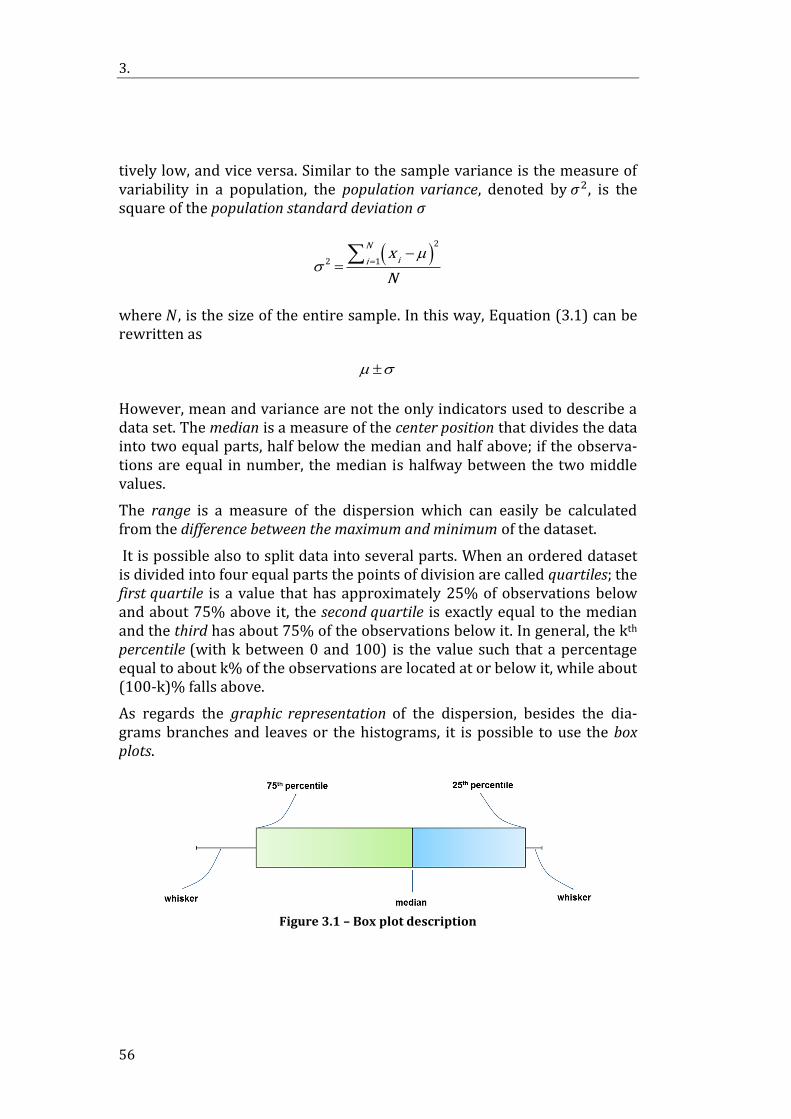
3.
56
tively low, and vice versa. Similar to the sample variance is the measure of variability in a population, the population variance, denoted by 𝜎2, is the square of the population standard deviation 𝜎
2
2 1
N
iix
N
where 𝑁, is the size of the entire sample. In this way, Equation (3.1) can be rewritten as
However, mean and variance are not the only indicators used to describe a data set. The median is a measure of the center position that divides the data into two equal parts, half below the median and half above; if the observa-tions are equal in number, the median is halfway between the two middle values.
The range is a measure of the dispersion which can easily be calculated from the difference between the maximum and minimum of the dataset.
It is possible also to split data into several parts. When an ordered dataset is divided into four equal parts the points of division are called quartiles; the first quartile is a value that has approximately 25% of observations below and about 75% above it, the second quartile is exactly equal to the median and the third has about 75% of the observations below it. In general, the kth percentile (with k between 0 and 100) is the value such that a percentage equal to about k% of the observations are located at or below it, while about (100-k)% falls above.
As regards the graphic representation of the dispersion, besides the dia-grams branches and leaves or the histograms, it is possible to use the box plots.
Figure 3.1 – Box plot description

Uncertainties in Thermoeconomic Input-Output Analysis
57
Such a representation describes simultaneously the most important fea-tures of the data sets, such as the center, the dispersion, the deviation from symmetry and the identification of observations that fall unusually far from the main group of data, the so-called outliers. A box plot (Figure 3.1) repre-sents the three quartiles aligned on a rectangular box. The box encloses the entire difference between the third and the first quartile with the lower side in correspondence of the 25th percentile and the upper of the 75th one. The middle line of the box is then drawn at the median. Outside of the opposite sides of the box stretch the whiskers; the lower one goes from the first quar-tile to the smallest observation within 1.5 interquartile difference, from the first quartile, while the upper whiskers is from third quartile to the largest observation within 1.5 interquartile differences, from the third quartile.
A mathematical model of a physical system need not necessarily to be a per-fect abstraction: incorporating uncontrollable variables or inaccurate in-formation, changes in the outcome measures are expected. The variables derived from the observations, the measured value of which may change from time to time, are defined random or aleatory variables, 𝑋. The proba-bility is a concept used to quantify the likelihood, or possibility, that a meas-urement falls within a given set of values. “The possibility that 𝑋, the cost of an asset, is between 5000 and 5200 € is equal to 95%” is a statement that quantifies the feeling about the possible costs of that particular asset. The probability of a result can be interpreted as the degree of subjective confi-dence in the fact that this result may appear. As the probability of a result is in terms of relative frequency (per unit of total observations), referring to the cost of the asset mentioned, the relative frequency of repeated observa-tions that fall in the range will be equal to 0.95. It can be written as
5000 5200 0.95P X
Not always an experiment produces a measured value and the values used in the models are not always derived from experimental observations. Sometimes a value can only be classified into a number of possible catego-ries. Well, the concept of probability is applied in these cases too, and the in-terpretation in terms of frequency is still adequate [1].
The densities are commonly used in engineering to describe physical sys-tems, similarly, a probability density function can be used to describe the probability distribution of a continuous random variable. The probability that 𝑋 falls between 𝑎 and 𝑏 is then determined as the integral of 𝑓(𝑥) from 𝑎 to 𝑏. The probability density function of a continuous random variable is used to determine the probability in the following way

3.
58
b
aP a X b f x dx
The probability density functions are characterized by positive functions, the probability can vary from 0 to 1 if, respectively, the values cannot occur or are certain. The function is used to calculate an area that represents the probability that the variable takes a value in the specified range. Further-more, it is possible to synthesize the probability distribution by its mean and its variance.
The most widely used model for the distribution of a random variable is un-doubtedly the normal distribution. It is also said Gaussian and has a sym-metrical bell shape; each time a random experiment is repeated, the ran-dom variable, that is equal to the average result or total of replicas, tends to assume a normal distribution with increasing the number of replicates. The expected value of the distribution determines the center of the probability density function, that of variance determines its width. A random variable with probability density function
2
221
2
x
f x e
has a normal distribution and is said normal random variable with parame-ters 𝜇 e 𝜎, the distribution is often indicated by the notation 𝑁(𝜇, 𝜎2). Since the probability density function decreases when moving away from the av-erage, the probability that a measurement falls far from the expected value is low and from a certain distance, respect to the average, onwards can be approximated to zero. The area under the graph of a normal distribution over a certain distance equal to 3𝜎 from the average is very small; since more than 99.73% of the probability of a normal distribution is within the range (𝜇 ± 3𝜎) as the width of the distribution is often indicated the value 6𝜎.
The variables of a system sometimes follow an exponential relationship as 𝑥 = 𝑒𝑤. Whether the exponent is a random variable, 𝑊, then 𝑋 is also a ran-dom variable. When 𝑊 has a normal distribution then the distribution of 𝑋 is said lognormal due to the calculation of the natural logarithm of 𝑋 which therefore also appears to have a normal distribution. When 𝑊 has mean 𝜃 and variance 𝜔2, 𝑋 = 𝑒𝑊 is a lognormal random variable with probability density function

Uncertainties in Thermoeconomic Input-Output Analysis
59
2
2
ln( )
21
2
x
f x ex
The parameters of a lognormal distribution are 𝜃 and 𝜔2 but these are just the mean and variance of the random variable 𝑊. The lifetime of a product that will degrade over time is often modeled as a lognormal random varia-ble.
There are also many other studied distributions, however, for the purposes of this thesis it may be more useful to turn an eye to simple distributions such as the range or the triangular one. The range, also known as uniform distribution, can simply be described by two variables: the minimum and the maximum values. This distribution is used when there is an equal probabil-ity that a quantity lies between a minimum and a maximum value [6].
When a value within the range has a higher probability to be observed the triangular distribution must be used. The latter is sometimes used as an al-ternative for the normal distribution, the advantage is that extremely high or low values cannot occur. As it is not said that the most probable value lies exactly in the middle of the range, this distribution can be used to approxi-mate asymmetrical distributions as well as the lognormal one.
Statistical uncertainty and sensitivity analysis aim at assessing the contribu-tions of the parameters uncertainties in contributing to the overall uncer-tainty of the model output [24]. Sampling-based analysis is performed in or-der to ascertain if model predictions fall within some region of concern and to identify the dominant parameters in contributing to the response uncer-tainty. The very first step of sampling-based analysis, in which uncertainties are assigned, is crucial to the results produced by the subsequent steps in the analysis because the results depend entirely on the distributions as-signed to the sampled parameters, hence, the proper assignment of these distributions is essential to avoid producing bogus results.
3.2. Processing data and model uncertainties
All types of uncertainty affect directly or indirectly (through the model) the input data and propagate up to the results, the model outputs. The uncer-tainty of the data can be treated by defining a disturbance, a perturbation that affect the average or nominal data. The propagation of uncertainty to the results can be studied by applying the Monte Carlo method. Especially in

3.
60
the case of an Input-Output analysis, the Monte Carlo method is suggested to treat the propagation of uncertainty amongst the mathematical struc-tures, such as matrixes and vectors, used. Lenzen [7] suggests that to assess the propagation of uncertainty in studies involving the Leontief inverse, the use of a Monte Carlo technique is necessary because it is not possible to car-ry out an analytical approach.
Besides, even using a sensitivity analysis of some assumptions globally, the changes performed on the input data, which continue to present some vari-ability, propagate in final results. So, once again the best solution for the analysis is that to combine Monte Carlo method for data uncertainties with sensitivities analysis for model uncertainties [6]. Descriptive statistics then may be useful to summarize and show more effectively the analyses results.
3.2.1. Perturbation theory
The theory on the influence of perturbation of coefficients of matrixes on so-lutions of system of equations, can be used in Input-Output analysis. The quantities that describe the processes in Input-Output tables and so the co-efficients that define the technology matrix often suffer from uncertainty. A statistical treatment of the propagation of these uncertainties is important even to investigate options for products improvement as such uncertainties affect ultimately results. However, the direct applicability of such approach is limited because the matrixes encountered in Input-Output analysis have particular characteristics, e.g. such matrixes are in most cases positive de-fined. Perturbation theory studies the influence of perturbations of equa-tions coefficients on the solutions to those equations [25]. For example, by considering Leontief’s production model expressed by Equation (3.2)
y I A x (3.2)
a typical question addressed in perturbation theory is, given the above sys-tem, what would the solution be when the matrix (𝑰 − 𝑨), which for straightforwardness of writing can be simply called 𝑨, is perturbed, ��
I A A
The Leontief’s matrix inversion on the perturbed matrix can be used to find the new solution recalculating it, but can be also interesting to study how

Uncertainties in Thermoeconomic Input-Output Analysis
61
the perturbation propagates in the system. For this, we will consider the perturbed matrix to consist of the original matrix plus a perturbation term
A A A
trying to derive expression for the solution perturbation term 𝛿𝒙, defined as
x x x It is possible to study the effects of such a change in technology matrix on the result vector 𝒙 starting from
y A A x x
Expanding the terms in parentheses
y A x A x A x A x
As 𝑨 𝒙 = 𝒚
0 A x A x A x
Assuming that �� is invertible
1 1( ) x A A A A y
This important relationship enables to explore the study of perturbation theory and statistical analysis of the Input-Output analysis. Under the hy-pothesis of 𝛿𝑨 infinitesimally small, 𝑨 + 𝛿𝑨 ≅ 𝑨, so
1 1
ij ij
a a
x AA A y (3.3)
In agreement with the differentiation rule for inverse matrixes (e.g. Balestra [26]), it results
11 1
ij ij
a a
A AA A

3.
62
This way Equation (3.3) becomes
1 11
ij ij ij ij
a a a a
x A y Ay A y
Thus, each coefficient of the vector 𝜕𝒙 𝜕a𝑖𝑗⁄ depends on the individual ele-
ments of 𝜕𝑨−1 𝜕a𝑖𝑗⁄ . The knowledge of these derivatives opens the way to
explore sensitivity and uncertainty analysis of all the derivatives 𝜕𝑥𝑘 𝜕a𝑖𝑗⁄
for each value of 𝑖 and 𝑗.
Another important concept of matrix perturbation theory is the condition number. By considering perturbations in vectors 𝒙 and 𝒚, the inequality for multiplications of norms yields
1 x A y
But also
y A x
Thus, by combining these two equations
1
x y
A Ax y
it is possible to measure how a relative change in 𝒚 propagates as a relative change in 𝒙. The factor
1 A A A
is known as the condition number of the matrix 𝑨; whenever such a number
is large, relative variation in the vector of results may be very higher than in 𝒚 and the solution of this kind of equations may be perturbed. A practical rule states that whenever the magnitude of a condition number is like 10d then, in the solution of the equation, one can obtain 𝑡 − 𝑑 correct digits, where 𝑡 represents the correct digits of input values. For instance, when the input data is correct to 3 decimal places, a condition number of 100 means that 2 decimal point are lost in the solution to a system of equations, so that

Uncertainties in Thermoeconomic Input-Output Analysis
63
the solution is correct to 1 decimal place only. So, when data are quite im-precise to only 1 or 2 decimal places, a technology matrix with a condition number of 10 or 100 would deprive the result from any certainty: uncer-tainties in data and their propagation in the computations is therefore of theoretical and practical interest.
Perturbations in thermoeconomic Input-Output analysis because of uncer-tainties, can occur in the construction of the exergetic table, for example considering that fuel flows may not have constant exergy because of the variability of the different consignments of fuel used in the system, while being of the same type. So a perturbation will be produced also in vector of final demand. Moreover, uncertainty can be in exogenous resources vector since, for example, different enterprises can produce resources with similar but different costs. In any case, the perturbation can be studied as shown.
By considering a single unit process described by a process vector as
1
2
p
pp
it is necessary to abandon the idea of point estimates, and include the idea that a distribution of values for the elements of this process vector exists. For simplicity, one can assume that this distribution is Gaussian. This ena-bles to describe the distribution with mean 𝜇 and standard deviation 𝜎. It is quite normal to write such a stochastic variable as 𝜇 ± 𝜎, although this nota-tion is sometimes used to indicate the range of possible values that the vari-able may attain. This way the process vector is
1 1
2 2
( , )
( , )
p p p
N
N
In principle, every process vector may be defined this way and a stochastic process matrix may be constructed.
This is a conservative procedure, as it is based on the idea that all uncertain-ties are independent but in practice, this is not true: just think of the uncer-tainties on the exergy of a input as a fuel and the consequent uncertainties in the exergy of the exhausted gases. At any rate, it is likely that not all un-certainties are independent. In general, the degree of dependence between

3.
64
two random variables is measured by their covariance, the covariance be-tween a variable and itself being the variance
2
1 1 1cov( )p , p
All the variances and covariances may be arranged in a matrix, the covari-ance matrix or dispersion matrix that is a symmetric matrix. The disad-vantages of using this construction are: the reduction of information due to this symmetry, the fact that a very large matrix is necessary to represent all variances and covariances. In practice, covariances are almost never availa-ble in an empirical form. Only theoretical considerations, for example, on the basis of mass balances and chemical reaction theory can provide esti-mates of covariances.
Describing data uncertainties is like describing data to a certain sense; next step, is describing how to combine the variability in data into an overall un-certainty. For the combination of uncertainties there are other trends in ad-dition to the distribution theory, as the categorical data quality description or the fuzzy set theory, but they are less used and there is not lot of litera-ture available about them. Hence, the main approaches are that based on parametric variation, on analytical expression for error propagation or on random experiments for uncertainty propagation as those that adopt Monte Carlo techniques.
3.2.2. Monte Carlo technique
Monte Carlo analysis is a sampling technique based on numerical simulation in which a sample of engineering model results is generated and statistical properties of this sample are used to provide an indication of the location and dispersion of the results [27]. While analytical method are exact, sam-pling techniques provide stochastic results that are not exactly reproduci-ble. However it should be noted that with analytical methods, approxima-tions are often needed and that several authors [7] point out that, for par-ticular models, such as those Input-Output, it is necessary to use random experiments for uncertainty propagation. Sampling techniques are able to deal with more than only a few theoretical distributions and can include all type of complicated dependencies. Especially when fast computers are avail-able, Monte Carlo techniques provide a useful means of assessing robust-ness. Thermoeconomic Input-Output analysis is an area where it may be applied fruitfully. Having specified probability distributions for process data, one can proceed to generate one model realization. This yields a vector of

Uncertainties in Thermoeconomic Input-Output Analysis
65
results e.g. 𝒄, that can be denote as 𝒄1. A second realization yields a second result 𝒄2, all together, after model realizations, a set of results {𝒄1, 𝒄2, … , 𝒄𝑁} will be obtained and this set of results can be subject to analyses. In per-forming a Monte Carlo analysis, one must choose the number of runs 𝑁. It is important to underline that the number of uncertain input parameters does not affect the number of runs required. The latter is only determined by the required accuracy of the output distribution and the computing capabilities available.
After Monte Carlo development in the first half of the twentieth century, the method was continually in use and became a prominent instrument in the development of many projects and soon, applications started popping up in all sorts of situations in business, engineering, science and finance [28]. It is clear, then, that one of the main aspects of the method is to have available a reliable random number generator. This is a computerized or physical method that produces numbers that have no sequential pattern and are ar-ranged purely by chance. Many computer languages have been developed to allow, in one way or another, to write codes for countless applications; lan-guages as Visual Basic were popular in developing computer simulation models. The number of simulation software packages has also exploded over the years. Software include mathematical equations and algorithms as-sociated with a given process. When the software fits the process under study, the user can apply it and quickly observe the outcomes from a new or modified arrangement of the process. This ability is a large saving in time and cost of development.
The models highly depend on the authenticity of the algorithms and on the choice of the input probability distributions and parameter values. An error in the formulation could give misleading results. Generating random num-bers with use of a computer is not easy. One of the first tools used to gener-ate random numbers is by way of the mathematical function called modular arithmetic. For a variable 𝑤, the modulo of 𝑤, modulus 𝑚, is denoted as 𝑤 𝑚𝑜𝑑𝑢𝑙𝑜(𝑚). The function modulo returns the remainder of 𝑤 when di-vided by 𝑚. When 𝑤 and 𝑚 are integers, the function returns the remainder that also is an integer. Such a method and its advancements are one of the most common technique in use.
A series of tests have been developed in order to evaluate how good a se-quence of uniform random variables are with respect to truly random uni-form variables. The first consideration is how many random variables are generated before the cycle repeats. When the generated random numbers are set in intervals, the frequency for every interval of the numbers and the expected number of generated random numbers in an interval may be eval-uated. With these two parameters a Chi Square (goodness-of-fit) test is used

3.
66
to determine if the sequence of generated numbers is spread equally in the considered range. Another test computes the autocorrelation between the generated random variables, the ideal is for all the autocorrelations to be significantly close to zero. These numbers are thereby called pseudo random numbers as they pretend to be random.
Whit the matrixes arrangement of an Input-Output analysis, the Monte Car-lo method is suggested to treat the propagation of uncertainty. Lenzen [7], believing necessary the use of a Monte Carlo technique, stated that uncer-tainties in matrixes, as that of the technical coefficient 𝑨, can be simulated by generating a matrix, 𝛿𝑨, which contains random perturbation. Moreover, Lenzen suggests that according to Quandt [29] it is possible to assume a normal distribution of uncertainty, even if Hanssen and Asbjørnsen [30] showed in their studies, that this is not always true. Moreover Kop Jansen [31] pointed out, because of the way Input-Output tables are constructed, uncertainties are correlated but the nature of this correlation and distribu-tion is usually not known.
3.2.3. Uncertainty analysis, some numerical example
Before proceeding with the description of the used methodology for uncer-tainty evaluation in thermoeconomic Input-Output analysis, two numerical example of perturbation theory are provided simply to see how perturba-tion and uncertainty affect Leontief’s production and cost models.
First, the uncertainty may affects the elements of the Input-Output table up to the technical coefficient matrix 𝑨. For example, by considering Leontief’s production model
1 A y x
1.0050 0.9870 13.15 25.61
0.0019 1.0856 12.56 13.66
the Leontief’s inverse comes from the Input-Output matrix
0.0835 12.3789
0.0447 1.0554
E
in accordance with the theory presented in Chapter 2. When a perturbation is introduced as

Uncertainties in Thermoeconomic Input-Output Analysis
67
0 10
0 0
E
such that
E E E
0.0835 2.3789 0.0835 12.3789 0 10
0.0447 1.0554 0.0447 1.0554 0 0
it propagates through Equation (2.15) up to the Leontief’s inverse in such a way as to cause that it can be expressed as
1 1 1 A A A
1.0036 0.1894 1.0050 0.9870 0.0014 0.7976
0.0019 1.0841 0.0019 1.0856 0.0000 0.0015
The condition number of the inverse is very low and equal to 3 so that the problem is not ill-conditioned. Hence, recalculating with the perturbed ma-trixes, the uncertainty reaches the result vector 𝒙 as it is observable
x x x
15.57 25.61 10.04
13.64 13.66 0.02
Next, for example in the Leontief’s cost model, the uncertainty may affect the exogenous resources vector
v v v
35.11 30.11 5
22.17 13.17 9
Since the specific cost are given, in accordance with Equation (2.14), by

3.
68
1T
c A b
1.18 1.0050 0.0019 1.18
2.21 0.9870 1.0856 0.96
in which the specific exogenous resources vector 𝒃 is defined via Equation (2.12), it is possible to evaluate the propagation of uncertainty through the vector 𝒃
b b b
1.38 1.18 0.20
1.62 0.96 0.66
up to the result, the cost vector
c c c
1.38 1.18 0.20
3.12 2.21 0.91
in which the perturbation is very different from that introduced as 𝛿𝐯. Fur-thermore, it should be mentioned that the uncertainties can affect the coef-ficients matrix and the resources vector at the same time with a propaga-tion of effects due to different causes. Also because very rarely a change of value in a matrix or in a vector of the thermoeconomic Input-Output ar-rangement is not correlated with other changes and a perturbation produc-es other perturbations in cascade even before the application of the equa-tions of the Leontief’s models.
3.3. A method for uncertainty evaluation in ther-
moeconomic Input-Output analysis
In this thesis the methodology used for the evaluation of the uncertainty in thermoeconomic Input-Output analysis is the Monte Carlo technique for three main reasons:

Uncertainties in Thermoeconomic Input-Output Analysis
69
1. to handle uncertainty not only infinitesimally small, the application of random experiments for uncertainty propagation is not subject to the limitations of the assumptions of the analytical approach;
2. to estimate the correlations and the dependencies amongst the ma-trixes arrangement, as it is not true that uncertainties are independ-ent;
3. as indicated by the specific scientific literature, the studies by Lenzen [7] and Bullard and Sebald [32] among others.
Bearing in mind the discussion set forth in Chapter 2 and in Subparagraph 3.2.3, the uncertainty can be considered proper to the values that form the Input-Output table or can affect the values that make up the exogenous re-sources vector. A variation of the values of exergy input to the system, for example due to the variability of the goods for which the plant is supplied as raw materials for its operation, is reflected on a variability that accompa-nies the outputs produced by the system; and so is, even if the uncertainty is own of the exergetic vector of external resources. Some uncertainties can be also typical of the values of the cost of the equipment composing the system; this is true in the design phase when comparing the different possibilities offered by the market and not, of course, when studying a system that is al-ready built, whit all costs known. But it is not always said that all the infor-mation required for the construction of this economic vector, even for an existing plant, can be known with certainty according to the resources available to the analyst. Furthermore, the degree of belief on the correct-ness of some information from assumptions on the model or the change in the definition of certain parameters of the model will result in uncertainties in the values of the results of the analysis.
Anyway, the variability can be represented thanks to the perturbation theo-ry: each vector affected by uncertainty may be expressed as for the exoge-nous resources vector by
v v v in which the perturbation 𝛿𝐯 may vary for every iteration of the 𝑁 Monte Carlo runs. The number of iterations may be chosen based on the typical values found in the scientific literature, for example Bullard and Sebald [32] [33] suggest that 1000 iterations would be sufficient, to mediate between the resources spent to produce them and the quality of the results obtained. Hence, 1000 runs are adopted
1 1 v v v
2 2 v v v
1000 1000 v v v

3.
70
From each iteration the results of the thermoeconomic Input-Output analy-sis are, then, derived also characterized by variability
1 2 1000, , , c c c c c c
The variability can be introduced using known information about the data. When one knows the range of variation of a parameter, for which each value within the interval is equally probable, the quantity can be expressed through a uniform distribution, the range. In Excel this can be done by the function RANDBETWEEN. Consequently also the results, arising from inputs distributed this way, will have an almost uniform distribution. The inclusion of the values of the output when all the input ranges are at the maximum and minimum value in this type of analysis is essential because it provides information that is not said that the random analysis can consider. However it is not possible to do without the random analysis by a Monte Carlo tech-nique because it simulates the propagation of more than one uncertainty up to results. A final definition of the interval as the output resulting from the minimum and maximum values of the input, it would not take into account a multiple propagation. Think of the definition of the thermodynamic variable f, the uncertainty of the exergoeconomic factor will result derived from un-certainty in investment costs plus that of the cost of the exergy destruction; with Monte Carlo simulations one does not risk to underestimate the range of variation of this result.
When it is possible to assume that the data distribution is normal, then the uncertainty in data may be described by the mean and the variance; in Excel the function NORMINV may be used together with the RAND function to simulate the probability and the results will be distributed according to the Gaussian distribution, evidently.
At each iteration, the output of the thermoeconomic Input-Output analysis, in Excel [34], can be stored by typing the command in Visual Basic to have, at the end of the simulations, all the results in order to proceed with their analysis. In addition to the graphic presentation by means of box plots, out-put may be described through drawing intervals with the representation of the quartiles in which the values of the studied results are included. In Fig-ure 3.2 a schematic representation of the passages for the application of the method is presented.

Uncertainties in Thermoeconomic Input-Output Analysis
71
Figure 3.2 – Monte Carlo method for Input-Output analysis diagram

72

73
4. Casalvolone Anaerobic Digester
The analyzed case study is an existing plant of anaerobic bio-digestion. This plant is taken as an example to show the application of the method of uncer-tainty evaluation in an thermoeconomic Input-Output analysis.
4.1. Introduction to anaerobic digestion
A biomass classification may be done on the quantity of water possessed: if the amount of water is lower than 50%, biomass will be classified as rela-tively dry; if the amount of water is greater than 80%, biomass will be cate-gorized as definitely moist; if the water is present in a percentage between 50 e 80%, it will be possible to decide whether to dilute the biomass in or-der to continue the treatment with a wet processing or to dry the biomass in order to use it as a fuel. Depending on the type of biomass, on the investa-ble capital and on the presence or absence of incentives it should be identi-fied the optimal process (dry or wet) for the production of energy. This pro-cess consist in the transformation of the chemical energy owned by the bi-omass in another form of available energy: thermal and/or electric energy. Transformations can lead to formation of not properly energetic byproducts (e.g. glycerol for the production process of biodiesel or digestate for the production process of biogas).
Besides the thermochemical (combustion, gasification, pyrolysis) and chem-ical (e.g. transesterification) processes, biologic processes, as the anaerobic digestion and the fermentation may convert the form of energy contained in the biomass in heat and work. If the water content in the biomass is high, when the energy consumption to dry the biomass is not justified or if the plant cost for the drying process becomes too high, the biochemical conver-sion represents the best way to exploit the energy content of the biomass and the anaerobic digestion is normally the adopted process.
4.1.1. Biomass digestion
The use of different types of dedicated and waste biomass has led to the de-velopment of various types of anaerobic digestion processes and different technologies, mainly based on the dry matter content of the substrate fed

4.
74
into the reactor [35]. Therefore, based on the total solids content, there are three different techniques:
1. wet digestion, when the substrate in the digestion has a dry sub-stance content below 10%, this is the most common technique, par-ticularly with animal slurry;
2. semi-dry digestion, with intermediate values of dry matter, 10-20%, this process is less common;
3. dry digestion, when the substrate in the digestion has dry substance content exceeding 20%.
The choice to work in separate or individual phases is subject to the charac-teristics of the substrate: highly biodegradable substrates are more difficult to manage with one-phase processes. The anaerobic microorganisms have low growth rate and low rate of reaction and therefore it is necessary to keep optimum the conditions of the reaction environment. The latter, usually defined anaerobic reactor, to allow the simultaneous growth of all the mi-croorganisms involved, shall result from a compromise between the needs of individual microbial groups.
The rate of net increase of digestion on a given substrate is a function of the internal temperature of the digester and the type of bacteria and the rate of use of biomass which depends on the concentration and the affinity be-tween bacteria and biomass. Increasing the concentration of substrate, it is possible to approach the maximum possible rate; other important parame-ters are pH (7-7.5 optimum value for the methanogenesis), alkalinity and the production and percentage composition of the biogas. The anaerobic bio-logical activity is possible in a wide temperature range, between –5 and +70 °C with various microorganisms classified according to the optimal thermal interval of growth:
psychrophilic bacteria (temperatures below 20 °C); mesophilic bacteria (temperatures between 20 °C and 40 °C); thermophilic bacteria (temperatures above 45 °C).
The activity of the bacteria, however, increases with temperature so that a higher temperature, becoming more rapid gas production, results in a lower retention time of the material inside the digester. On average, with meso-philic bacteria 16-30 days are necessary, while with thermophilic bacteria the range decreases to 14-16 days. The choice of temperature then comes from a compromise between gas production and possible maximum tem-perature, which must be such as not to destroy the enzymes; so insulations and systems for heating the biomass within the digester are used.

Casalvolone Anaerobic Digester
75
The percentage of methane in the produced biogas varies, depending on the type of digested biomass and on the conditions in the reactor, from a mini-mum of 50% to a maximum of 80%. The biomass subjected to anaerobic di-gestion is defined by a few parameters easy to measure like:
· the total solids or dry substance (% on wet basis) is the dry matter content, determined by drying at 105 °C and representing the sum of the organic substance and the inert substance;
· the volatile matter (% of dry matter) is the fraction of organic matter that can volatilize, about 80% of the total organic, operationally it is assumed that the volatile substance is equal to the organic matter.
The biomass conversion leads to degradation of the sugars, even of cellulose, through various reactions that produce a biogas consisting primarily of me-thane and carbon dioxide and digestate (the material remaining from biode-gradable feedstock after the digestion that produce biogas). Schematically, four key biological and chemical stages happen:
1. hydrolysis, the complex organic molecules are broken into simple sugar, amino acids and fatty acids;
2. acidogenesis, there is further breakdown of remaining components into volatile fatty acids, ammonia, carbon dioxide and hydrogen sul-fide;
3. acetogenesis, simple molecules are further digested to produce large-ly acetic acid, as well as carbon dioxide and hydrogen;
4. methanogenesis, bacteria digest the acids into methane, carbon diox-ide and water.
For the success of the process of methanisation is important the retention time, or the residence time, defined as the residence time of the organic mass in the digester. The biogas production increases with the retention time: initially zero, within a few days reaches the maximum and then de-creases slowly with a bell-shaped trend. The hydraulic retention time 𝜏 rep-resents the residence time of each fluid element within the reactor or the average of the residence times in the reactor of the individual fluid ele-ments.
,
reactor
F IN
V
V (4.1)
where 𝑉𝑟𝑒𝑎𝑐𝑡𝑜𝑟 is the volume of the reactor, ��𝐹,𝐼𝑁 is the volumetric flow rate
of the total amount at the reactor inlet and the retention time is usually ex-pressed in days.

4.
76
Several biomasses, treatable anaerobically, have a content of sulfur com-pounds that is not negligible for the purposes of the digestion process. The main form of sulfur compounds is that of sulfate, which, in the environment of the strongly reducing anaerobic reactor, is soon converted into sulphide. The presence of sulfur compounds promotes the growth of sulfate reducing bacteria that compete with methanogenic bacteria in the use of acetic acid and hydrogen.
In wet processes the biomass is treated so as to have a total solids content less than 10% in order to be able to use a classic continuous agitated-tank reactor. The biomass, before being loaded into the anaerobic reactor, un-dergoes a treatment aimed at achieving a proper content of total solids and of a good level of homogenization; it consists mainly of a dilution carried out by addition of water (slurry and/or process water) and of a removal of any foam, plastics or other coarse materials which are potentially damaging to the mechanics of the plant. The reactor most frequently used in this type of process is the classic continuous stirred-tank reactor (CSTR).
4.1.2. Stages of a digestion plant
Firstly near the farm is realized a storage site, where the livestock manure, collected through a mechanical recovery manure system, and the vegetal biomass are stored and accumulated. It is important to avoid that in this site reactions which lead to the formation of methane can occur and so the de-tention time in the storage site must be as low as possible. Any methane production would be, in fact, very harmful, not only for the possible envi-ronmental pollution, but also because it would reduce the methane produc-tion in the digester itself, thus going to reduce also the overall efficiency.
Anaerobic digestion is a process of biological conversion, in oxygen absence, through which approximately 50% of the organic substance contained in the input matter is transformed into biogas consisting in methane, carbon dioxide and traces of water, nitrogen, hydrogen and pollutants. The digester can be single or double-stage, and can be characterized by a cold digestion or by a heated digestion. The choice is at the discretion of the designer and depends on the process parameters to optimize. To choose a configuration over another one availability of biomass, financial resources, infrastructure, space, sanitation requirements, climate (because a cold climate requires better insulation) and time of storage must be taken into account. Within the reactor, the substrate in the digestion phase should be properly mixed, so as to: facilitate contact between bacteria and substrate, avoid the pres-ence of dead zones, ensure a homogeneous temperature distribution, opti-

Casalvolone Anaerobic Digester
77
mize the release of biogas and prevent settling of the sludge and the for-mation of surface crusts. The mechanical agitators are generally subject to abrasion and clogging, due to the presence of hard or fibrous particles, and therefore they require frequent maintenance.
The digestate is collected and stored in tanks; it can be used as soil improv-er, downstream of a chemical-physical analysis aimed to detect within it the presence of possible contaminants to the soil. The positive outcome of the analysis allows the direct use of digestate as fertilizer in agriculture, other-wise it is necessary to establish a system of digestate treatment.
The operation of the equipment connected to the biogas must be continuous while the diagram of the production may be subject to temporal variations. It is therefore necessary to have a storage system with a volume able to equalize the fluctuations of production so as to not having to stop the ma-chines of the plant or release the gas in the torch to prevent dispersion in the environment. The gas storages, also called gas holders, have variable volume and low pressure that can be variable or constant.
The biogas, after undergoing the treatments required to reduce the presence of moisture, sulfur compounds and particulates, is controlled and sent to electrical power production. The electricity generated in cogeneration is fed into the electricity grid via a parallel connection with the alternator. In the event the grid has a voltage different from that of the electricity produced, it is necessary to raise it by means of a transformer substation.
In the design of the anaerobic digestion units, it is also necessary to pay at-tention to the construction aspects related to the system of charging and discharging the mixture from the digester and to the handling of sludge. The loading/unloading system must be made in such a way that, introduction of air mass in the reactor and leaks of matter or of biogas from the reactor does not occur. The unloading system must allow the dosage of the digested material to the next stage of the process. It must be thus provided a control system which prevents accidental emptying of the digester during unload-ing. Irrespective of the loading/unloading system, the digester must be equipped with a protection system to the pressure and the vacuum.
4.2. Description of Casalvolone digester
The analyzed existing anaerobic digester is that in Casalvolone in the Prov-ince of Novara, Piedmont. This is one of the more than 500 agricultural bio-

4.
78
gas plants present nowadays in Italy [36]. Public incentives for electricity production and heat valorization from biogas are granted, so biogas is uti-lized to feed combined heat and power generation plant (CHP) engine. Ac-cording to Fantozzi and Buratti [37] Casalvolone plant reactor can be ana-lyzed as a CSTR. As in plants of other European countries the usage of cereal silage, regarding the feeding of reactor, is accompanied by digestion of ani-mal manure, this represents one of the best technique for an energy valori-zation of this byproducts, moreover this lead to a reduction of methane emission during storage of manure.
4.2.1. Main features
Casalvolone plant has an installed power of 999 kWel and co-digests maize silage and pig slurry respectively in percentage of 54.5 and 45.5%. The CHP engine of the plant has electrical and thermal efficiencies such that the 40.7% of the power available to the engine (as biogas heating value) is con-verted into electricity and the 44.0%, instead, is converted into heat availa-ble as hot water. Figure 4.1 shows the main components of the plant.
Figure 4.1 – Casalvolone plant diagram, main components
The maize is stored in silos at the biogas plant, where it is ensiled. This bio-mass is transported from the field to the biogas plant with farm tipping trailers. The transport of pig slurry is done by sludge tanks. During ensiling and storage operations, some biomass is lost, in fact, a maize loss of 2% is considered while for pig slurry no losses occur, considering that it is moved through pipelines. In the loading phase the solid biomass is fed into the di-gester through a screw auger, which requires 65 kW, placed on the bottom of a hopper in which the maize silage is loaded by tractor coupled with a frontal loader. Pig slurry is introduced in the digesters by means of a pump

Casalvolone Anaerobic Digester
79
requiring 20 kW. The water utilized for dilution of feedstock is introduced using a pump requiring 15 kW; so within the reactor, dry matter content is about 10%.
Inside the two digesters the temperature is kept in mesophilic conditions to 40 °C by hot water coming from the engine jacket. Such a water is moved by 4 pumps, entailing 1.5 kW consumption, in the heat exchangers on the di-gester wall. Single-stage digestion takes place in continuous stirred-tank re-actors. Furthermore, each digester has submerged mixers with an electrical power of 13 kW for homogenization of feedstock and liquid fraction and a pump for the digestate discharge requiring 22 kW. The biogas produced as a result of the digestion of organic matter is stored in the gasholder dome placed on the top of the digester.
The biogas that leaves the reactor is filtered in a sand filter, dehumidified and desulfurized. Dehumidification is due to a refrigeration unit of 15 kW which cools down the biogas temperature removing the water vapor while desulfurization is due to NaOH in a wet scrubber that requires 10 kW.
Energy conversion occurs in the CHP unit that runs constantly at 1500 rpm and where biogas is burnt in an internal combustion engine with an electri-cal power generation of 999 kWel and a thermal one of 1100 kWth. More precisely, the CHP recovers the heat from both the engine water cooling jackets (at about 70 °C) and the exhaust gases (at 150 °C). Maize silage and pig slurry properties have been studied experimentally by Fiala [38] and are reported in the following Table 4.1
Biomass Total solids Volatile solids Produced biogas Methane in biogas
% of wet bases % of total solids m3N/t volatile solids % volume
Pig slurry 3.5 85 450 60 Maize silage 38.0 90 650 53
Table 4.1 – Characteristics of biomass
Considering such characteristics, a dilution of the maize silage is required, it is carried out with water that can come from liquid fraction of digestate. One ton of feedstock mixture corresponds with about 0.9 t of digestate; the latter can partially be separated into solid and liquid fraction and it is spread in the fields as organic fertilizer. Every day in the digester are intro-duced 55 t of maize silage, 45 t of pig slurry end 120 t of water for dilution on wet basis and, always on a daily basis, are produced by the plant 203 t of di-gestate. According to Dressler et al. [39] biogas losses from digesters, biogas treatment devices and CHP can be estimated in the order of 1.5%. Methane losses can be quantified for this plant equal to 91.5 m3N/day on a total bio-gas production of 11438 m3N/day; the subscript N is referred to normal

4.
80
conditions of temperature and pressure at 273.15 K and 101325 Pa. In Ta-ble 4.2 gross and net production and self-consumption of electricity and heat may be observed
Gross production Self-consumption Net production
Electricity (kWhel/d) 23982 1758 22224 Heat (kWhth/d) 25927 8303 17624
Table 4.2 – Electricity and heat production
Specific heat consumption per produced biogas is 0.726 kWhth/m3N, while, per produced net electricity it is equal to 0.373 kWhth/kWhel.
4.3. Plant thermodynamic model
From information provided by the study of Bacenetti et al. [36] the thermo-dynamic model of the Casalvolone anaerobic digestion plant has been con-structed. Here it is presented in stages of the conversion process: load, di-gesters, biogas treatment and power production. Then, the main and funda-mental exergy flows have been evaluated.
4.3.1. Loading stage
The mass flow rate of the maize is 0.63 kg/s, that of slurry 0.53 kg/s with a flow rate of water equal to 1.39 kg/s. In Table 4.3 the mass fractions of the feedstocks are indicated.
Feedstock y
Maize 0.25 Slurry 0.21 Water 0.54
Table 4.3 – Mass fractions of feedstocks
Hence, the total flow rate has been calculated by the sum of the three feed-stocks to the value of 2.55 kg/s (220 t/d). Once familiar with the percentage of the dry solid fraction of the maize and the slurry, it can be concluded that 62% of maize and 97% of the slurry is made of moisture. By considering the aforementioned maize loss ∆��𝑚𝑎𝑖𝑧𝑒,𝑑𝑟𝑦 through equation
,dry ,dry(1 )
maize maize maize maizem m m y

Casalvolone Anaerobic Digester
81
a mass flow rate of dry maize of 0.23 kg/s (20.3 t/d) has been evaluated. Similarly flow rate of dry slurry is found to be equal to 0.02 kg/s (1.6 t/d) and that of water plus the biomasses moistures to 2.29 kg/s (197.7 t/d) via
,tot ,dry ,dry(1 ) (1 )
water maize maize slurry slurry waterm m y m y m
Thus, as said, it has been possible to estimate the dry mass fractions of the feedstocks, as shown in Table 4.4,
Feedstock y dry
Maize 0.09 Slurry 0.01 Water 0.90
Table 4.4 – Dry mass fractions of feedstocks
in order to verify that only 10% of feedstock consists of dry matter capable of producing biogas.
The evaluation of the heating value of the biomasses deserves a separate discussion. The elemental chemical composition of the maize has been as-sumed from Fiala [38] and is presented, on dry basis, in Table 4.5. From such a composition, by knowing the percentage of dry fraction and by nor-malizing results, it has been possible to estimate the mass fraction of all chemical elements; moreover, inasmuch as
1
i
i i
Mmy
Mm
; i i
i
Mmx y
Mm
with 𝑀𝑚, molar mass of the maize equal to 6.4 kg/kmol, also mole fractions 𝑥𝑖 of all elements have been estimated and all the results are in Table 4.5.
Element y dry y x
C 0.429 0.163 0.087 H 0.073 0.097 0.618 O 0.481 0.733 0.294 N 0.002 0.001 0.000 S 0.001 0.000 0.000 Cl 0.002 0.001 0.000 Ash 0.012 0.005 0.000
Table 4.5 – Elemental composition of maize
Through a Dulong empirical relationship [40] the higher heating value of the maize has been so calculated

4.
82
32.79 150.4 9.26 4.97 2.428
OC H S O N
yHHV y y y y y
(4.2)
at the value of 9.8 MJ/kg as the empirical coefficient in Equation (4.2) are expressed in such units. As regards the slurry, instead, since there are no studies on its elemental composition, it has been necessary proceed with the assumptions from the composition of the solid faeces. These assumptions are justified by the fact that 97% of the pig slurry is composed of water, so they only affect a small percentage of the total composition of this feed-stock. Faeces are mainly composed by fiber, bacteria, fat, protein, and sub-stances that can be classified as ashes in percentages and compositions that can be deduced from scientific literature. For example, for the fatty acids, from stearic to oleic one, passing through all the different types, composi-tions in terms of carbon, oxygen and hydrogen are known, thus it has been possible to estimate the average mole compositions and so for all constitu-ents of the faeces. The elemental chemical composition utilized in this thesis for the pig slurry is hence reported in Table 4.6. This way, to evaluate the higher heating value of the slurry Equation (4.2) has been applied to obtain 5.1 MJ/kg. Once evaluated biomasses HHVs the power of feedstock mix into the reactors has been calculated on the value of 4500 kW through the rela-tion
, ,dry ,dry ,dry ,dryF IN maize maize maize slurry slurry slurryQ m y LHV m y LHV
where the lower heating value of dry biomasses have been estimated, by considering the dry mass compositions and the evaporation enthalpy of wa-ter, to the values of 17.0 MJ/kgdry and 22.5 MJ/kgdry respectively for the maize and the slurry.
Element y dry y x
C 0.421 0.015 0.007 H 0.073 0.111 0.663 O 0.320 0.868 0.328 N 0.017 0.001 0.000 Ash 0.170 0.006 0.001
Table 4.6 – Elemental composition of slurry
The retention time has been considered to be equal to 20 days in accordance with an article of Campi et al. [41]. The volumetric flow rate of the feedstock mix introduced into the reactor has been estimated to be equal to 261.6 m3/d as the used densities are equal to 568 kg/m3, 1000 kg/m3 and 999 kg/m3 respectively for the maize, the slurry and water. This way, through

Casalvolone Anaerobic Digester
83
Equation (4.1) the volume of the reactor has been calculated to 5231 m3. Thanks to an interview to a technician of the EnviTec Biogas, the manufac-turing company of the plant, it has been discovered that the reactors have a standard form of 25 m in diameter and 6 m in height. Thus it is clear that the total amount of the volume is considered be split into 2 reactors.
4.3.2. Digestion stage
In the reactors, a fraction of biomass becomes biogas, such conversion has not been studied through a discussion centered on the set of chemical reac-tions that occur in the digester, but taking into consideration the infor-mation present on the experimental production of methane from biomasses by Fiala [38] shown in Table 4.1. In Table 4.7 is presented the composition (mole fractions) assumed and estimated of the biogas
Molecule xmaize xslurry
CH4 0.530 0.600 CO2 0.413 0.343 H2O 0.044 0.044 H2S 0.003 0.000 H2 0.001 0.004 N2 0.010 0.010
Table 4.7 – Molecular composition of biogas by different biomasses
Where the fraction of the methane is known and that of the carbon dioxide is derived as a complement to one, since the CO2 is the main component of biogas together with CH4, while the fractions of water and hydrogen sulfide have been estimated from an article of Bacenetti and Negri [42]. The frac-tion of hydrogen has been assumed while the nitrogen one comes from a technical report of an anaerobic digester plant by Giommi [43]. The total volumetric flow rate of biogas has been calculated by multiplying the mass flow rates of biomasses by the percentages of volatile solid and by the con-version factors of produced biogas, all shown in Table 4.1 to get a value of 12482.2 m3N/d (0.14 m3N/s). To undertake an evaluation of the total com-position of the biogas, the flow rates of biogas from the maize and from the slurry have been expressed in mole terms through
biogas N
biogas
N
V pn
R T
to obtain 529.7 kmol/d (0.0061 kmol/s) and 27.2 kmol/d (0.0003 kmol/s), respectively. In this way, it has been possible to evaluate the mole flow rates

4.
84
for each chemical species and for each biomass of the plant. Through the es-timation of the molar mass of the biogas in the digesters
i ii
Mm x Mm
to the value of 27.7 kg/kmol, the composition of biogas at the exit of the reac-tors has been calculated and results are shown in Table 4.8.
Molecule ṅ
(kmol/s) x y
ṁ (kg/s)
CH4 0.0034 0.53 0.31 0.0552 CO2 0.0026 0.42 0.65 0.1161 H2O 0.0003 0.04 0.03 0.0051 H2S 0.0000 0.00 0.00 0.0006 H2 0.0000 0.00 0.00 0.0000 N2 0.0001 0.01 0.01 0.0018
Table 4.8 – Composition and flow rates of biogas at reactor exit
The conditions in the reactor are a temperature of 313.15 K [36] and a pres-sure of 500 Pa [43]. Since the saturation pressure of water at this tempera-ture is equal to 7384 Pa, no vapor slip occur within the biogas, or rather, the flow rate of water within the biogas flow does not change. Thus, the flow rate of biogas can be expressed in mole quantities to 556.9 kmol/d (0.0064 kmol/s) or in mass quantities at 0.1787 kg/s (15.4 t/d) at reactor exit. From the digesters also the digestate comes out, simply as a difference coming from mass balance at the reactor
,digestate F IN biogas reactorm m m
Its mass flow rate is equal to 204.6 t/d.
4.3.3. Biogas treatments stage
In accordance with Bacenetti and Negri’s article [42] it is possible to derive the removal efficiencies of water vapor and of sulfur from biogas: efficiencies of 95% and 97%, respectively, have been assumed. The treatments in the dehumidifier and in the desulfurizer produce variations in the composition of the biogas, at the end of these processes, the composition is that observa-ble in Table 4.9 with a molar mass of 28.1 kg/kmol.

Casalvolone Anaerobic Digester
85
Molecule ṅ
(kmol/s) x y
ṁ (kg/s)
CH4 0.0034 0.56 0.32 0.0552 CO2 0.0026 0.43 0.67 0.1161 H2O 0.0000 0.00 0.00 0.0003 H2S 0.0000 0.00 0.00 0.0000 H2 0.0000 0.00 0.00 0.0000 N2 0.0001 0.01 0.01 0.0018
Table 4.9 – Composition and flow rates of biogas at biogas treatments exit
Hence, mole flow rate at the end of treatments has been evaluated to the value of 0.0062 kmol/s and mass flow rate to the value of 0.1733 kg/s. In this stage, according to Bacenetti et al. [36] a 1% biogas loss has been con-sidered. This has led to a reduction of the flow rates to the values of 527.0 kmol/d (0.0061 kmol/s, 11811.7 m3N/d) and 14.7 t/d (0.1716 kg/s). The lower heating value of the treated biogas has been calculated equal to 15.9 MJ/kg via
i ii
LHV y LHV
considering the mass composition of biogas and the LHV of each chemical species.
4.3.4. Power production stage
In accordance with another article by Bacenetti et al. [44] the daily availabil-ity of the CHP engine has been considered equal to 21.92 h. Also taking ac-count of the abovementioned relative loss on the 0.5% in conversion of bio-gas into the engine, and of an absolute one regarding methane fraction, the actual flow rates of fuel input to the CHP engine have been evaluated: a mole flow rate of 471.5 kmol/d (0.0055 kmol/s) and a mass flow rate of 13.3 t/d (0.1535 kg/s). As the 41% of biogas power (LHV) is converted into electri-cal power and the 44% in thermal power, by multiplying mass flow rate by LHV of biogas for these two efficiencies, gross electrical and thermal powers have been estimated to the values of 995 kW and 1076 kW respectively. By considering all the auxiliaries, the power for the screw auger of maize, for the pumps of slurry, feed-water and hot water for the reactor, for agitators of reactor, for digestate handlings, for dehumidifier, for desulfurizer and for the blower of biogas, a needed power of 207 kW has been estimated, so, the net power produced by the plant can be evaluated to 789 kW. Taking ac-count of a 32% self-consumption of thermal power [36] even the net thermal power produced by the digestion plant has been calculated to the value of

4.
86
732 kW. Also the produced energies per time unit have been estimated by considering the obtained results, for a comparison with the data of the real plant, and a 7.5% self-consumption of electricity [36], the results are shown in Table 4.10
Gross production Self-consumption Net production
Electricity (kWhel/d) 23884 1791 22093 Heat (kWhth/d) 25821 8263 17558
Table 4.10 – Calculated electricity and heat production
The specific heat consumption per produced biogas has been assessed to the value of 0.782 kWhth/m3N and the specific heat consumption per produced net electricity to 0.374 kWhth/kWhel. Accordingly, the gotten results, start-ing from the actual data of the system and from the assumptions made in the model, agree with the data gathered in the existing plant.
Different efficiencies of Casalvolone plant have been evaluated. Regarding the heating value of the biomasses,
,
netel
F IN
W
Q
the electrical efficiency to 18%, considering the ratio between net electrical power of the plant and the power entering the system with the biomasses.
,
netth
F IN
Q
Q
The thermal efficiency to a value of 16%, considering the net thermal power.
,
net netI
F IN
W Q
Q
The first law efficiency as sum of the first two.
0
ln,
,
1net net
th
II
F IN
TW Q
T
Q

Casalvolone Anaerobic Digester
87
The second law efficiency, getting the value of 19%, takes into account the quality of the output produced by the plant by weighting the thermal power with Carnot factor. Where the average temperature of the flow has been evaluated at a temperature of 336.71 K using the expression
, ,
ln,
,
,
ln
IN exc OUT exc
exc
IN exc
OUT exc
T TT
T
T
as a thermal user inlet temperature of 85 °C and an output one of 43 °C have been assumed. Regarding the heating value of the biogas, instead, with anal-ogous expressions have been calculated the values of 32%, 30%, 62% and 36% respectively for electrical, thermal, first and second law efficiency. Fi-nally, the index of energy saving, IRE, has been estimated to the value of 12% through
,CHP
,ref ,ref
1 biogas
net net
el th
m LHVIRE
W Q
where the reference electrical, 𝜂𝑒𝑙,𝑟𝑒𝑓, and thermal efficiencies, 𝜂𝑡ℎ,𝑟𝑒𝑓, to the
values of 40% and 90%, have been derived from Italian electricity and gas Authority [45] [46].
4.3.5. Estimating exergy flows
For the evaluation of the exergy flows, a simplification on the conception of the plant structure, which leads to the analysis of the main nine components, has been performed, in a fuel and product logic. The nine components taken into consideration are: the screw auger, the water pump, the slurry pump, the digesters, the digestate tanks, the dehumidifier, the desulfurizer, the blower with the filter and the control system and, at last, the CHP engine. In each component, there are input and output exergy flows both linked to ma-terials flows and to energy flows, but, among these, only those which consti-tute a useful output for the component and the system are taken into ac-count; e.g. the flow of condensate exiting the dehumidifier or the flow of ex-haust gases from CHP engine have not been considered. In Table 4.11 are

4.
88
shown the compositions and the conditions of the mass flows from which exergy flows have been estimated as exposed in Table 4.12.
Table 4.11 – Mass composition and condition of mass flows
y
C
yH
y
O
yN
y
S
yC
l y
Ash
p
(P
a)
T
(°C
) ṁ
(k
g/
s)
Ma
ize
IN
pla
nt
0.1
63
0
.09
7
0.7
33
0
.00
1
0.0
00
0
.00
1
0.0
05
1
01
32
5
25
0
.63
1
Ma
ize
IN
re
act
or
0.1
63
0
.09
7
0.7
33
0
.00
1
0.0
00
0
.00
1
0.0
05
1
01
32
5
25
0
.61
8
Wa
ter
IN p
lan
t -
0.1
12
0
.88
8
- -
- -
25
00
00
1
5
1.3
89
W
ate
r IN
re
act
or
- 0
.11
2
0.8
88
-
- -
- 1
15
00
00
2
5
1.3
89
S
lurr
y I
N p
lan
t 0
.01
5
0.1
11
0
.86
8
0.0
01
-
- 0
.00
6
10
13
25
2
5
0.5
27
S
lurr
y I
N r
ea
cto
r 0
.01
5
0.1
11
0
.86
8
0.0
01
-
- 0
.00
6
60
13
25
2
5
0.5
27
B
iog
as
IN d
eh
um
idif
ier
0.4
08
0
.08
1
0.4
97
0
.01
0
0.0
03
-
- 5
00
4
0
0.1
79
B
iog
as
IN d
esu
lfu
rize
r 0
.42
0
0.0
80
0
.48
7
0.0
10
0
.00
3
- -
33
3
5
0.1
74
B
iog
as
IN b
low
er
0.4
21
0
.08
0
0.4
88
0
.01
0
0.0
00
-
- 2
00
1
5
0.1
73
B
iog
as
IN C
HP
en
gin
e
0.4
21
0
.07
9
0.4
89
0
.01
0
0.0
00
-
- 2
00
00
4
2
0.1
54
D
ige
sta
te I
N t
an
ks
0.0
16
0
.11
0
0.8
71
0
.00
0
0.0
00
0
.00
0
0.0
03
1
01
32
5
40
2
.36
8
Dig
est
ate
OU
T p
lan
t 0
.01
6
0.1
10
0
.87
1
0.0
00
0
.00
0
0.0
00
0
.00
3
10
13
25
2
5
2.3
68
N
aO
H I
N d
esu
lfu
rize
r -
- -
- -
- -
10
13
25
2
5
0.0
01
N
a2S
OU
T d
esu
lfu
rize
r -
- -
- -
- -
10
13
25
2
5
0.0
02
H
ot
wa
ter
OU
T p
lan
t -
0.1
12
0
.88
8
- -
- -
24
50
97
8
5
1.9
58
A
ir I
N C
HP
en
gin
e
- -
0.2
33
0
.76
7
- -
- 1
01
32
5
25
1
.33
9
Ta
ble
4.1
1 –
Ma
ss c
om
po
siti
on
an
d c
on
dit
ion
of
ma
ss f
low
s

Casalvolone Anaerobic Digester
89
Table 4.12 – Enthalpy, entropy and exergy flows
Δ
fH°
(kJ/
kg
) h
(k
J/k
g)
H
(kW
) S
° (k
J/k
gK
) s
(kJ/
kg
K)
S
(kW
/K
) e
ch
(kJ/
kg
) e
ph
(kJ/
kg
) e
(k
J/k
g)
E
(kW
)
M
aiz
e I
N p
lan
t -1
21
00
0
.00
0
.00
5
.25
0
.00
0
.00
1
01
63
0
.00
1
01
63
6
41
0
M
aiz
e I
N r
ea
cto
r -1
21
00
0
.00
0
.00
5
.25
0
.00
0
.00
1
01
63
0
.00
1
01
63
6
28
2
W
ate
r IN
pla
nt
-15
86
5
-41
.70
-5
7.9
2
3.8
8
-0.1
4
-0.2
0
17
3
0.8
7
17
4
24
2
W
ate
r IN
re
act
or
-15
86
5
-40
.84
-5
6.7
2
3.8
8
-0.1
4
-0.2
0
17
3
1.7
7
17
4
24
3
S
lurr
y I
N p
lan
t -1
54
39
0
.00
0
.00
4
.00
0
.00
0
.00
1
16
1
0.0
0
11
61
6
12
Slu
rry
IN
re
act
or
-15
43
9
-1.1
1
-0.5
8
4.0
0
-0.0
2
-0.0
1
11
61
6
.09
1
16
7
61
5
B
iog
as
IN d
eh
um
idif
ier
-76
29
4
0.2
1
7.1
9
7.1
3
1.7
2
0.3
1
16
41
8
-47
3.8
8
15
94
4
28
50
Bio
ga
s IN
de
sulf
uri
zer
-74
70
-2
4.6
4
-4.2
9
7.0
4
1.6
0
0.2
8
16
86
8
-50
2.5
5
16
36
5
28
46
Bio
ga
s IN
blo
we
r -7
49
4
-24
.64
-4
.27
7
.04
1
.75
0
.30
1
68
48
-5
47
.65
1
63
00
2
82
5
B
iog
as
IN C
HP
en
gin
e
-74
94
2
2.7
9
3.5
0
7.0
4
0.5
5
0.0
8
16
84
8
-14
2.1
8
16
70
6
25
65
Dig
est
ate
IN
ta
nk
s -1
50
66
6
0.5
8
14
3.4
2
4.4
2
0.2
0
0.4
7
12
46
1
.47
1
24
7
29
53
Dig
est
ate
OU
T p
lan
t -1
50
66
0
.00
0
.00
4
.42
0
.00
0
.00
1
24
6
0.0
0
12
46
2
95
0
N
aO
H I
N d
esu
lfu
rize
r -1
06
46
0
.00
0
.00
1
.61
0
.00
0
.00
2
11
2
0.0
0
21
12
3
Na
2S
OU
T d
esu
lfu
rize
r -7
44
7
0.0
0
0.0
0
4.1
5
0.0
0
0.0
0
83
17
0
.00
8
31
7
18
Ho
t w
ate
r O
UT
pla
nt
-15
86
5
49
1.9
8
49
1.9
8
3.8
8
0.7
7
1.5
0
17
3
22
.48
1
96
3
83
Air
IN
CH
P e
ng
ine
0
0
.00
0
.00
6
.74
0
.00
0
.00
4
0
.00
4
5
Ta
ble
4.1
2 –
En
tha
lpy
, en
tro
py
an
d e
xe
rgy
flo
ws

4.
90
The specific enthalpies and entropies per mass unit have been estimated by using the software REFPROP of US NIST (National Institute of Standards and Technology). For the estimation of these quantities, for maize dry fraction, it has been necessary to define an equivalent fuel gas which would ensure the reckon with such a software, because the latter does not work with the ele-mental compositions of fuels. In order to ensure the equivalence between the maize dry fraction and the fictitious gaseous fuel it has been verified that the atomic populations and the heating values of the two were identical (exactly equal to 18.7 MJ/kg and to composition in Table 4.13).
Element y
C 0.436 H 0.074 O 0.489
Table 4.13 – Elemental and actual composition of equivalent fuel (dry maize)
The only assumption made is that of considering maize dry fraction as com-posed only of carbon, oxygen and hydrogen, i.e. neglecting the other ele-ments with a less important weight. The specific enthalpy has been there-fore calculated as the weighted average, on the mass fractions, of the wet and dry contributions.
.1
maize water dry eq F drymaize
h h y h y
The enthalpies, for maize and for all other flows in the plant, have been cal-culated using REFPROP and as differences between those assessed from the conditions given in Table 4.11 and those evaluated considering the refer-ence conditions (298.15 K and 101325 Pa), in such a way to make the esti-mates independent from the reference. The exact same procedure has also been used to calculate the entropies of the flows. As regards the physical ex-ergy, it has been derived from the expression
0 0 0
ph h h T s s e (4.3)
used for maize and for all other flows. By considering the standard chemical exergy of components of equivalent fuel and of liquid water from Kotas [47] the chemical exergy of maize has been assessed with a weighted mean on mass wet and dry fractions. For maize as for all streams the standard en-thalpy of formation and the standard entropy were evaluated from the NIST
Molecule x y
CH4 0.458 0.285 CO 0.263 0.286 CO2 0.215 0.367 H2O 0.033 0.023 O2 0.031 0.038

Casalvolone Anaerobic Digester
91
data. Total exergy has been assessed as the sum of chemical and physical exergy, and therefore the exergy flow rates have been derived directly from the multiplication of this by the mass flow rate.
ph ch
fm m E e e e (4.4)
The maize which enters reactors differs from that entering plant just for the maize loss already discussed as shown in Table 4.11 and Table 4.12.
Regarding feed-water, it has been considered at the plant inlet a tempera-ture (15 °C) lower than the reference, taking into account that part (in case of use of the liquid fraction of the digestate) or all of this water could come from the water network. For the same reason a pressure of 2.5 bar has been assumed as the average pressure of the aqueduct. Enthalpy and entropy have been calculated through the software and exergy using Equations (4.3) and (4.4). The procedure for the calculation of chemical exergy, for water and the other flows, is the same used for maize and always passes for the values of the standard chemical exergy. The effect of the pump on the water flow at the entrance of the reactor has been evaluated by considering an in-crease of pressure of about 9 bar, taken from the data booklet of some manu-facturers of pumps, according to the parameter of flow rate of about 5 m3/h.
In the case of the slurry the problem of calculating of the flow of exergy has been approached as with maize. In this case, however, has not been neglect-ed any fraction of elemental analysis (as the nitrogen and ashes are more abundant in dry fraction and therefore relevant, see Table 4.6) and there-fore the equivalent fuel with the same atomic population is that reported in Table 4.14.
Element y
C 0.507 H 0.087 O 0.386 N 0.020
Table 4.14 – Elemental and actual composition of equivalent fuel
(dry slurry without ash)
The heating value of equivalent fuel has been assessed to the value of 24.5 MJ/kg. The procedure for the calculation of the thermodynamic quantities is the same already used for maize, except that, this time in the weighted av-erage has been considered the contribution of the ashes. The enthalpy and entropy of the ash has been evaluated with the use of the coefficients of
Molecule x Y
CH4 0.456 0.331 CO 0.477 0.604 CO2 0.000 0.000 H2O 0.046 0.037 N2 0.016 0.020 O2 0.005 0.008

4.
92
NASA (National Aeronautics and Space Administration) polynomial expres-sions based on JANAF (Joint Army Navy Air Force) data since it has been in-calculable with the software used. For the evaluation of the flow of slurry entering the reactor has been considered the increase in pressure of 5 bar generated by the pump in accordance with the information from the data booklet of manufacturers of pumps, function of the parameter of flow rate of about 2 m3/h.
The flow of the biogas leaving the reactors, described in Table 4.8, has been evaluated with the calculation of thermodynamic conditions of temperature and pressure reigning in the reactor via software. The exergy evaluation has been performed as already discussed for the other flows, considering the presence of gaseous species only, obviously.
The composition and flow rate of dehumidified biogas has been estimated based on the known information, mass and mole fractions of gas are given in Table 4.15.
Molecule x y
CH4 0.556 0.317 CO2 0.427 0.667 H2O 0.002 0.002 H2S 0.003 0.004 H2 0.001 0.000 N2 0.010 0.010
Table 4.15 – Composition of dehumidified biogas
The conditions of temperature and pressure presented in Table 4.11 for the dehumidifier, on the basis of which thermodynamic parameters have been evaluated, have been deduced from the technical catalog of an industrial dehumidifier which considers the operation of the chiller and a pressure drop of 40 mm of water column.
The flow of the biogas leaving the desulfurizer, described in Table 4.9, has been evaluated with the calculation of thermodynamic conditions of tem-perature and pressure obtained from a technical report of a similar plant [48].
Regarding the biogas at the entrance of the CHP engine, the value of pressure has been estimated from the data from Giommi’s technical report [43]. Through the knowledge of the flow rate and of the pressure value has been possible to estimate the rise in temperature consequent to the activity of the blower by reading diagrams of some technical catalogs of blowers.
The estimate of exergy flows of the digestate has been carried by consider-ing first of all its composition: this product is, in fact, given by the difference

Casalvolone Anaerobic Digester
93
between the feedstock mix introduced in the system and biogas leaving the reactor as shown in Table 4.16.
Element ydry y x
C 0.157 0.016 0.008 H 0.092 0.110 0.661 O 0.722 0.871 0.330 N 0.004 0.000 0.000 S 0.001 0.000 0.000 Cl 0.002 0.000 0.000 Ash 0.025 0.003 0.000
Table 4.16 – Elemental composition of digestate
Neglecting the contribution of nitrogen, sulfur and chlorine an equivalent fuel has been estimated to calculate the enthalpy and entropy of the flow; the calculated higher heating value of gaseous fuel and dry fraction without ash taken into account is equal to 9.3 MJ/kg and the compositions are shown in Table 4.17. The contribution of the ash has been taken into ac-count through the use of NASA polynomials and the assessment has been performed as already described for the slurry. The exergetic flow exiting the digestate tanks has been evaluated similarly but considering a temperature of 25 °C.
Element y
C 0.161 H 0.095 O 0.744
Table 4.17 – Elemental and actual composition of equivalent fuel
(dry digestate without ash)
Thanks to the NIST data for the sodium hydroxide, necessary for the capture of sulfur, it has been possible to evaluate the thermodynamic parameters of the flow in input to the desulfurizer. The flow rate has been calculated from known data considering the capture reaction
2 2 22 2H S NaOH Na S H O
For the byproduct output of the desulfurizer, the water and the sodium sul-phide has been considered with the composition shown in Table 4.18.
Molecule x y
CH4 0.184 0.145 CO 0.090 0.123 CO2 0.000 0.000 H2O 0.593 0.523 O2 0.133 0.209

4.
94
Molecule y x
Na2S 0.684 0.333 H2O 0.316 0.667
Table 4.18 – Composition of desulfurizer byproduct output
The thermodynamic parameters have been estimated as a weighted mean of the contribution of water (software) and sodium sulfide (NIST data).
The flow of hot water generated by the CHP engine has been evaluated by knowing the self-consumption of the thermal power generated by the plant through the equation
,
, ,
self consumption
water H
water IN exc OUT exc
Qm
c T T
by taking into account an inlet temperature of 85 °C and an output one of 43 °C for the heat exchanger of the reactor.
Finally, the exergy flow that accompanies the air required for combustion has been evaluated taking into account the combustion reactions
4 2 2 22 2CH O CO H O
and less significantly
2 2 2 2
3
2H S O SO H O
2 2 2
1
2H O H O
and considering a ratio of 3.76 between the nitrogen mole and the oxygen one and a 60% air excess consistent with data derived from the data sheet of the Jenbacher gas engine installed in the system.
4.4. Plant economic model
The plant economic model has been built according to the approach and methods of Bejan et al. [4] and Peters et al. [49]. To complete a system anal-ysis, in fact, an estimation of the major costs of the plant is important con-

Casalvolone Anaerobic Digester
95
sidering various assumptions and predictions referred to economic and technological environment and using engineering economics techniques. The cost is the amount of money to acquire or produce a good. The market price is usually affected not only by production cost, but also by other factors as demand, supply, competition, regulation and subsidies. Very important, es-pecially in a design analysis, is the cost of a final product. The total cost of a good is composed by fixed and variable costs. The term fixed identified those costs that do not change strongly with the production rate like for de-preciation, insurance, maintenance. Variable costs are those costs that vary more or less directly with the volume of the output like for materials, fuel, labor, electricity.
In this thesis each component of the plant or the plant itself outputs have been considered to have an economic cost given by the sum of fuel cost (maize silage and pig slurry), cost of capital investment and cost of operating and maintenance (O&M) for the particular component/plant under exam yielding the output.
4.4.1. Estimating total capital investment
In contrast to fuel and O&M costs, an investment cost is a one-time cost. The capital necessary to purchase the land, build all the required facilities and purchase and install the needed equipment for a plant is called fixed capital investment (FCI). The latter is the total system cost assuming an overnight construction, viz. a zero-time design and construction period. The total capi-tal investment (TCI) is the sum of the fixed capital investment and other out-lays. These ones may be:
· startup costs, are mainly associated with design changes that happen after completion of construction but before the system can operate and include labor, materials, equipment and even loss of income while the system is not operating;
· working capital, consists of the amount of money invested in items as raw materials, fuels, finished products in stock, cash kept on hand for operating expenses and/or taxes, required to pay for the operat-ing expenses before payment is received by products selling;
· costs of licensing, research and development; · allowance for funds used during construction, represents the amount
of money disbursed without obtaining any revenue in the period be-tween the beginning of design and the system startup.

4.
96
The fixed capital investment consists of direct and indirect costs. Direct costs are those costs of all permanent equipment, materials, labor and other resources involved in the construction and installation of the permanent fa-cilities. Components of direct costs are purchased equipment (PEC) cost and installation, costs of piping, instrumentation and controls, electrical equip-ment and materials, land, architectural work and service facilities as water. Indirect costs are costs required for the orderly completion of the project like those of engineering and supervision, for developing the detailed plant design and perform supervision and inspection; construction, including contractor’s profit and all the expenses for temporary facilities and opera-tions, tools and equipment, home office personnel located at the construc-tion site, insurance; contingencies, to face unplanned expenses due to weather, work stoppages, transportation difficulties.
For the case study, based on the Ravano Green Power (the company that operates the plant) declarations to the press in 2011 [50] a FCI of 4000000 € has been assumed. Clearly this estimate is valid at the time it were devel-oped. Because values like this one may have changed considerably with time due to changes in economic conditions (as inflation or deflation), some method must be used for updating cost data at a past date to costs that are representative of conditions at later time. That is why cost indexes are used. A cost index is an index value for a given time showing the cost at that time relative to a certain base time. By knowing the cost at some time in the past, it is so possible to determine the equivalent cost at present by multiplying the original cost by the ratio of the present index value to the index value applicable when the original cost was obtained, i.e.
present
present original
original
IC C
I
This way, the FCI of Casalvolone plant has been taken to the value of the reference year for this study, 2013. Through the Intratec Chemical Plant Construction Index the indexes have been estimated to the values of 156.6 and 165.5 respectively for 2011 and for 2013; so, the FCI has been evaluat-ed to 4184576 €.
Estimating the cost of purchased equipment is the first step in any detailed cost estimation. It is plain that the accuracy of cost estimates depends on the amount and quality of the available information and the budget and time available for making estimates. The best cost estimates may be done directly by vendors. The next best sources of cost estimates are those by ex-perts, who know costs for professional experience or through calculations

Casalvolone Anaerobic Digester
97
using the extensive cost databases often maintained by engineering compa-nies. Another method is that of using estimating charts obtained through the correlation of a large number of cost and design data. In a typical cost-estimating chart, when all logarithms of available cost data are plotted ver-sus the logarithms of equipment size, the data correlation results in a straight line in a given capacity range. The slope of this line, 𝛼, represents the important parameter known as scaling exponent, so, in equation, it gives
xx y
y
XC C
X
(4.5)
Hence, the purchase cost of an equipment, 𝐶𝑥, at a given capacity or size ex-pressed by 𝑋𝑥, may be estimated when the purchase cost of the same equipment, 𝐶𝑦, at a different capacity or size, expressed by 𝑋𝑦, is known.
The variable representing capacity or size is the primary design variable or combination of variables characterizing the size of the equipment in ques-tion. As in the absence of other cost information, an exponent value of 0.6 can be used, this approach is known as the six-tenths rule. Usually the value of scaling exponent are given for different equipment as a function of capac-ity range of the equipment.
In case study, since study aim is not to perform an economic analysis of a new facility or to study with precision the real costs of Casalvolone plant but to have a case, as realistic as possible, to build a thermoeconomic analy-sis and, above all, demonstrate the use of the methodology for the evalua-tion of uncertainty associated with this type of analysis, for the estimation of the costs in question simplified relationships have been used. These ex-pressions are obtained using typical values for the various cost categories; in particular the Equations (4.6) and (4.7) are derived from Bejan et al. [4]
1,47TCI FCI (4.6)
4,30FCI PEC (4.7)
So, as a first estimate, it is possible to originate the total capital investment even after assessing the purchased equipment cost. Knowing the fixed cost investment of existent plant, the TCI has been estimated swiftly by Equation (4.6) to the value of 6151327 €.
For the evaluation of the costs of purchased equipment constituents the nine components, in which the plant has been simplified since the exergy flows

4.
98
analysis, it has been necessary to proceed this way. As it has not been possi-ble to obtain the real cost of the loading systems from operators of the exist-ing plant, these have been derived from information of screw auger and pumps vendors before being corrected using Equation (4.5). For the screw auger, the variable 𝑋 used has been the mass flow rate while for the pumps the volumetric ones; scaling exponents assumed are 0.99 and 0.33 respec-tively for screw auger and for pumps [49]. All purchased equipment costs results are shown in Table 4.19.
Component PEC (€)
Screw auger 2607 Pump water 3761 Pump slurry 5181 Digesters 83721 Digestate tanks 51163 Dehumidifier 94452 Desulfurizer 62968 Blower, filter and control 9445 CHP 659859
Table 4.19 – Purchased equipment costs
Digesters and digestate tanks costs have been obtained from an interview with a technician of EnviTec Biogas as a range of values between 160000 and 200000 € for the reactors and between 90000 and 130000 € for the tanks, because of the variability linked to the inconvenience or various problems such as those associated to the status of the land where plant stands or to the specific requirements of the customer. Therefore, the cen-tral value of the interval has been assumed but, because the interviewed technician has interpreted these values as including the costs of the excava-tion, the land stabilization, but also the installation of the panels and piping, and all necessary ancillary equipment, in fact, these are not true PEC, so, to reach the actual utilized values in the analysis, Equation (4.7) has been used. The cost of the CHP engine has been derived from price lists of Jen-bacher, manufacturer of Casalvolone engine, considering a machine with the same power and efficiency. The purchased equipment costs of the other three components have been obtained by difference, (they have been allocat-ed according to the power required by the specific component) because no other data were available, by knowing the total value of the PEC by Equation (4.7) of 973157 €.

Casalvolone Anaerobic Digester
99
4.4.2. Fuel and operating and maintenance costs
Fuel costs are usually part of the O&M costs but, for their importance in thermal systems are considered separately. For the case study cost of maize silage and pig slurry (Table 4.20) have been estimated through the infor-mation from databases which take into account their variability during the year.
Feedstock CF
(€/t)
Maize silage 42.8 Pig slurry 3.3
Table 4.20 – Feedstock cost
By dividing these quantities by the heating value of each feedstock, through their sum, the cost of input mix necessary to the system can be achieved to value of 0.039 €/kWh.
The operating and maintenance costs may be divided into fixed and variable costs. The fixed O&M costs are composed by costs for operating labor, maintenance labor and materials, overhead, administration and support, distribution and marketing, research and development. The fixed O&M costs in the case study have been evaluated by considering those known of an akin plant plus an insurance cost of 2500 €/y while the variable O&M costs have been assumed equal to 0.009 €/kWh (𝑐𝑣𝑎𝑟𝑖𝑎𝑏𝑙𝑒
𝑂&𝑀 ) by comparison with those of other plants using renewable and conventional fuels. The value of the fixed O&M cost is 122.5 €/kW (𝐶𝑓𝑖𝑥𝑒𝑑
𝑂&𝑀 ), a value of an order of magnitude
higher than the average of conventional plants.
4.4.3. Cost economic evaluation
As known, an euro in hand today is worth more than a euro received one year from now because the euro in hand now can be invested for the year. Hence, as the cost evaluation of a plant requires comparisons of money transactions at various periods of time, methods are needed to account for the value of money over time. If a present value 𝑃 is deposited into an ac-count earning 𝑖 percent interest per time period and the interest is remitted at the end of each of 𝑛 periods, the account will increase to a future value 𝐹 as expressed by the relationship
F 1n
P i (4.8)

4.
100
Interest is the compensation paid for the use of borrowed money, in engi-neering economy it is expressed in percentage or as a decimal and the unit of time is the year. To calculate the real rate of return of an investment, first of all, the discount rate has been estimated. Indeed, it has been speculated that the plant was paid for the 60% with equity capital and 40% with debt capital; by considering interest on the debt of 3% and a rate of return on cap-ital debt of 10%, the discount rate has been estimated at 7.2%. The real rate of return, in a first approximation, is given by the difference between the discount rate and the inflation rate. Taking into account an inflation of 1.5% the real rate of return in question has been calculated to 5.7%.
An annuity is a series of equal amount of money transactions happening at equal time periods (year). The annuity term is the time from the beginning of the first time interval to the end of the last time interval. When 𝐴 euro are deposited at the end of each period in an account earning 𝑖 percent per pe-riod, the future sum is given by
1 1F
ni
A i
(4.9)
The present value of an annuity is defined as the amount of money that would have to be invested at the beginning of the present period at an effec-tive rate of return per period to yield a total amount at the end of the annui-ty term equal to the amount of the annuity. By combining Equations (4.8) and (4.9) it results
1 1
1
n
n
iP
A i i
The reciprocal of this factor is the capital recovery factor
1
1 1
n
n
i iCRF
i
that is used to determine the equal amounts 𝐴 of a series of 𝑛 money trans-actions, the present value of which is 𝑃. For the case study, a CRF of 0.085 has been calculated considering a useful life of 20 years.
Thus, the annual TCI cost has been evaluated through

Casalvolone Anaerobic Digester
101
TCIZ CRF TCI obtaining 523314 €/y; while for the O&M costs has been used
& & &
variable
O M O M O M
fixed Z C c H W
obtaining 193572 €/y, in which 𝐻 is the operating time in hours per year, 8000 for Casalvolone plant. This way, the estimate of the hourly costs of the nine components has been performed via
&TCI O Mj
j
PEC Z ZZ
PEC H
and obtained results are reported in Table 4.21.
Component Ż
(€/h)
Screw auger 0.24 Pump water 0.48 Pump slurry 0.35 Digesters 7.71 Digestate tanks 4.71 Dehumidifier 8.70 Desulfurizer 5.80 Blower, filter and control 0.87 CHP 60.76
Table 4.21 – Components costs
As costs may change during all plant lifetime, levelization can be used to ex-press the relationship between the value of the expenditure at the begin-ning of the first year and an equivalent annuity or levelized value. The con-cept of levelization is general and is defined as the use of time value of mon-ey arithmetic to convert a series of varying quantities to a financially equiv-alent constant quantity, the annuity, over a specified time interval. Levelized cost of electricity, LCOE, is the price at which electricity must be generated to get break even over the lifetime of the project. LCOE is, generally, used in calculating the costs of generation from different sources, it is assessed in-cluding cost of fuels together with cost of capital investment and O&M as euro per unit of energy, in fact, electricity generation in the year in question is the quantity used at the denominator of the equation

4.
102
&
,
1
1
1
1
TCI O MnF t t t
tt
nt
tt
C Z Z
iLCOE
W
i
With a production of 7961326 kWh/y, for the existing plant, has been esti-mated an LCOE equal to 0.19 €/kWh, a value that is amongst the highest compared with other renewable end conventional plants.
4.4.4. Profitability evaluation
An estimation of the expected profit from the investment is essential before capital is invested. In profitability evaluation profits and costs that will occur in the future are considered. The associated risks and uncertainties can be significant. In this study three parameters have been considered among all those available in economics: the net present value (NPV), the payback pe-riod (PBP) and the internal rate of return (IRR).
Net present value is the sum of the present discounted values of the cash flows over plant lifetime both incoming and outgoing; it represents the amount of money expected at the end of useful life of plant. When it is used for project selection any project with negative present value is rejected and if two projects are mutually exclusive, the one with the highest present val-ue is accepted.
The simple profitability analysis carried out considers an overnight invest-ment cost (that is for the year 0 considering the year 1 as the first year in which the plant starts earning). The capital investment is the only cash out-flow in the year of construction while from the first year in which the plant begins to yield products cash outflows are the costs of maintenance and feedstocks (949796 €/y). The revenues (1751492 €/y) are represented by the multiplication of the generated energy by the incentive. The latter has been estimated according to the tariff of current laws: equal to 0.180 €/kWh for plants that use bio-based products (such as maize) and 0.209 €/kWh for plants using bio-based byproducts (such as pig slurry) plus a premium, respectively, equal to 0.040 €/kWh and 0.010 €/kWh to take into account cogeneration benefit if it is present in a small scale cogeneration units and, especially, if the primary energy savings amounted to over 10% [51]. In the case in which bio-based byproducts are used together with bio-based products, with a percentage of the latter not exceeding 30% by

Casalvolone Anaerobic Digester
103
weight, the tariff and premium used are those for byproducts, so for Casal-volone plant an incentive of 0.220 €/kWh has been assessed. For the in-vestment has been considered a straight-line depreciation for 20 years (209229 €/y); taxes are equal to the gross cash flow multiplied by the as-sumed 34% tax rate (201439 €/y). Thus, from net cash flows, the discount-ed cash flows can be calculated by the well-known expression
,
1
tdis t t
CFCF
i
and those cumulative ones can be evaluated too as shown in Table 4.22.
Year CFdis (€)
ΣCFdis (€)
0 -4184576 -4184576 1 567887 -3616689 2 537263 -3079426 3 508291 -2571135 4 480881 -2090254 5 454949 -1635306 6 430415 -1204891 7 407204 -797686 8 385245 -412441 9 364470 -47971 10 344816 296845 11 326221 623067 12 308629 931696 13 291986 1223683 14 276241 1499923 15 261344 1761267 16 247251 2008518 17 233917 2242435 18 221303 2463738 19 209369 2673107 20 198079 2871186
Table 4.22 – Discounted cash flows
Therefore, the net present value is equal to 2871186 €. From Table 4.22 even the payback period can be evaluated as about 10 years since it is the length of time required for the cash inflows to recover the original cash out-lays required for the initial investment.
At last the internal rate of return has been calculated. The IRR method seeks to avoid the arbitrary choice of an interest rate, indeed, it calculates an in-terest rate internal to the system project in question. This way, the rate which makes the net present value of an investment zero, the internal rate of return, is determined iteratively. For the case study has been assessed to

4.
104
13.1% by using Excel IRR function. It represents the rate of interest earned on the time varying, unrecovered balances of an investment such that the final investment balance is zero at the end of the plant lifetime.
4.5. Introducing uncertainties
The quality of an analysis depends considerably on the data gathering man-aged. In case study the known real data of the Casalvolone plant have been complemented, when necessary, with secondary data or assumptions. Data concerning maize and transport related activities were collected by means of survey on farms and by interviews with the farmers; concerning the pig slurry, data regarding transport activities were collected via interviews with the owner of the biogas plant by Bacenetti et al. [36]. So also for information concerning operation of plant, such as biomass consumption, biogas pro-duction, electricity and heat requirement, was achieved through plant moni-toring and average data corresponding to the operation in one year (2012) was managed.
All other data have been estimated by the database, data sheets, charts, ta-bles, reports and materials in general made available by the Department of Agriculture of the University of Milan (2013), with the exception of those taken from the aforementioned interview with the company manufacturer technician of the plant. This way, it is easy to understand the degree of un-certainty that can characterize data available from so many different sources.
4.5.1. Uncertainties introduced in the study of the digester
In order to have a model such as to apply the proposed method of evalua-tion of uncertainty, for simplicity, it has been chosen to take account of the variability in the cost of the feedstock and of the components making up the plant. Just because the cost of maize silage and the pig slurry have been con-sidered, in economic model, as the mean value between those variables in the course of the year, it has been easy to assess the associated variability. The same can be said regarding the costs of the digesters and digestate tanks that have been provided from the interview to the company manufacturer technician just as ranges of values. To estimate the uncertainty that accom-panies other plant components, it has instead resorted to the recommenda-tions in Peters et al.’s text [49]. Indeed, for definitive estimates, based on

Casalvolone Anaerobic Digester
105
almost complete data, like that of pig slurry cost, a suggested accuracy is within ±10%; for a scope estimate based on sufficient data to permit the es-timate to be budgeted the probable uncertainty is within ±20%; for a study estimate based on knowledge of major items of equipment, like that of desulfurizer, a variability within ±30% has been considered. Hence, for the nine components of the plant, using a relative uncertainty the variability of costs is shown in Table 4.23.
Component CF ZTCI+ZO&M Total
Screw auger 17% 20% 17% Pump water 20% 20% Pump slurry 10% 20% 11% Digesters 11% 11% Digestate tanks 18% 18% Dehumidifier 30% 30% Desulfurizer 30% 30% Blower, filter and control 30% 30% CHP 20% 20%
Table 4.23 – Relative uncertainties of plant components costs
The total relative uncertainty of each component has been assessed by con-sidering the three components of cost, feedstocks (fuels), the capital in-vestment and operating and maintenance costs.

106

107
5. Case study thermoeconomic Input-Output analysis
Bearing in mind the theory outlined in Chapter 2, and considering all the variables evaluated in Chapter 4 thermoeconomic Input-Output analysis has been performed on the model of Casalvolone plant. By considering the theo-ry exposed in Chapter 3, moreover, the methodology of uncertainty evalua-tion has been applied in this type of analysis.
5.1. Existing case analysis
First, the thermoeconomic Input-Output matrix of exergy flows has been built starting from the nine components making up the plant. Then, for the existing case, a thermoeconomic Input-Output analysis has been performed for the evaluation of exergetic and exergoeconomic costs.
5.1.1. Thermoeconomic matrix set-up
Figure 5.1 shows the main interrelationships amongst the components of the plant.
Figure 5.1 – Simplified plant diagram

5.
108
With the exception of the traced rectangular which represents the boundary of the system, all components are connected by solid lines, those indicating the material flows, and dashed lines, those corresponding to the flows of heat, Q, and work, P, energy. The values of these exergy flows are all known from thermodynamic analysis of the system and are given in Table 5.1. For heat flows of course, the corresponding exergetic one has been evaluated through Carnot factor as already shown in the previous chapters.
Exergy flow Symbol Matrix
element Value (kW)
Maize IN plant E_01 E01 6410 Maize IN reactor E_14 E14 6282 Water IN plant E_02 E02 242 Water IN reactor E_24 E24 243 Slurry IN plant E_03 E03 611 Slurry IN reactor E_34 E34 615 Biogas IN dehumidifier E_45 E45 2850 Biogas IN desulfurizer E_56 E56 2846 Biogas IN blower E_67 E67 2825 Biogas IN CHP engine E_78 E78 2565 Exhaust gas OUT plant E_80 E80 174 Digestate IN tanks E_49 E49 2953 Digestate OUT plant E_90 E90 2950 Water OUT plant E_50 E50 1 NaOH IN desulfurizer E_06 E06 3 Na2S OUT plant E_60 E60 18 Air IN CHP engine E_08 E08 5 Power IN screw auger P_81 E81 65 Power IN pump water P_82 E82 15 Power IN pump slurry P_83 E83 20 Power IN reactor P_84 E84 58 Thermal power IN reactor Q_84 E84 39 Power IN digestate tanks P_89 E89 22 Power IN dehumidifier P_85 E85 15 Power IN desulfurizer P_86 E86 10 Power IN blower P_87 E87 2 Power OUT plant P_80 E80 789 Thermal power OUT plant Q_80 E80 84
Table 5.1 – Exergy flows for matrix set-up
As it can be seen, each flow is accompanied by two numbers, the first repre-sents the number of the component from which is coming out and the sec-ond is the number of the component to which is going in; 0 stands for the environment. In Table 5.1 is even showed the correspondence with the ele-ment of the matrix in question, evidently when more than a flow is indicated in the same position in the matrix this means that more than a flow rests on that component so it is simply necessary to sum up all the same elements; e.g. the reactor receives electrical and thermal power from the CHP engine,

Case Study Thermoeconomic Input-Output Analysis
109
P_84 and Q_84, the element E84 is given by the sum of these two contribu-tions. The matrix 𝑬 is so constructed
0 0 0 E14 0 0 0 0 0 0 0 0 E24 0 0 0 0 0 0 0 0 E34 0 0 0 0 0 0 0 0 0 E45 0 0 0 E49
𝑬 = 0 0 0 0 0 E56 0 0 0 0 0 0 0 0 0 E67 0 0 0 0 0 0 0 0 0 E78 0 E81 E82 E83 ΣE84 E85 E86 E87 0 E89 0 0 0 0 0 0 0 0 0
It is a square matrix 9 × 9, since 9 are the components. By considering also the exergy exchanges with the environment, the vector of the outputs to the environment is constructed considering only the exergy flows accompanying products that represent the actual products engendered by the production system (final demand), namely electrical and thermal power, the sulphur output from the desulfurization process and the digestate; the vector is therefore made up as
𝒚𝑒𝑛𝑣𝑇 = 0 0 0 0 0 E60 0 ΣE80 E90
The vector that represents the inputs coming from the environment to the plant (exergetic exogenous resources), instead, is
𝒗𝑒𝑛𝑣 = E01 E02 E03 0 0 E06 0 E08 0
Moreover, two other vectors can be constructed considering the sums of the elements by row and column (from 0 to 9), those of total outputs and inputs
𝒙𝑇 = ΣE1j ΣE2j ΣE3j ΣE4j ΣE5j ΣE6j ΣE7j ΣE8j ΣE9j
𝒘 = ΣEi1 ΣEi2 ΣEi3 ΣEi4 ΣEi5 ΣEi6 ΣEi7 ΣEi8 ΣEi9
By the Equation (2.15) the technical coefficients matrix has been estimated
0 0 0 1.083 0 0 0 0 0 0 0 0 0.042 0 0 0 0 0 0 0 0 0.106 0 0 0 0 0 0 0 0 0 1.001 0 0 0 1.001
𝑨 = 0 0 0 0 0 1.001 0 0 0 0 0 0 0 0 0 1.101 0 0 0 0 0 0 0 0 0 2.293 0 0.010 0.062 0.033 0.017 0.005 0.004 0.001 0 0.007 0 0 0 0 0 0 0 0 0

5.
110
and so, the Leontief inverse matrix has been calculated too
1.032 0.190 0.100 1.187 1.205 1.217 1.343 3.079 1.212 0.001 1.007 0.004 0.046 0.047 0.047 0.052 0.119 0.047 0.003 0.019 1.010 0.116 0.118 0.119 0.131 0.301 0.119 0.029 0.176 0.093 1.097 1.113 1.125 1.240 2.844 1.119
(𝑰 − 𝑨)−1 = 0.029 0.175 0.092 0.097 1.112 1.123 1.239 2.841 0.118 0.029 0.175 0.092 0.097 0.112 1.122 1.237 2.837 0.118 0.027 0.159 0.084 0.088 0.101 0.111 1.123 2.576 0.107 0.012 0.069 0.037 0.038 0.044 0.048 0.054 1.123 0.047 0.000 0.000 0.000 0.000 0.000 0.000 0.000 0.000 1.000
The condition number of such a matrix is 37, a relatively low value which involves the loss of one significant digit in results at most. So, the problem is not particularly ill-conditioned.
5.1.2. Exergy cost analysis and evaluation
Through equations from Subparagraphs 2.2.1 and 2.2.2 an exergy cost anal-ysis has been performed on the basis of matrixes arrangement explained. The exogenous resources vector consists of exergy flow. For each compo-nent the amount of exergy destruction has been evaluated and the results obtained are shown in Table 5.2.
Component Edes
(kW)
Screw auger 193 Pump water 14 Pump slurry 17 Digesters 1434 Digestate tanks 25 Dehumidifier 18 Desulfurizer 17 Blower, filter and control 262 CHP 1451
Table 5.2 – Exergy destruction
As shown, the major irreversibilities occur in the components where the main energy conversions take place, in the digesters with the conversion from the feedstock mix to biogas and in CHP engine with the conversion from biogas to electrical and thermal power. The other two, in order of im-portance, major values of exergy destruction are those of the components in which the principal decreases in mass flow rate occurs (due to material loss) with a consequent reduction of the exergy flows.

Case Study Thermoeconomic Input-Output Analysis
111
The exergetic efficiencies of the nine components are displayed in Figure 5.2 (see Appendix for all numerical results).
Figure 5.2 – Exergetic efficiencies of plant components
All components have high efficiencies except the CHP engine, in which con-version processes should be enhanced to reduce irreversibilities. Next, by multiplying Leontief inverse matrix by the the exergetic specific exogenous resources vector, the specific exergetic costs of product per unit of exergy have been evaluated as presented in Figure 5.3. Each cost, expressed in J/J (or kWh/kWh), is the exergetic expense to produce 1 J (or 1 kWh) of exergy accompanying the output flow of the component in question. The values are all slightly above 1 and, as to be expected, they grow along the chain of the conversions in the system, even if, for the CHP engine the value of the cost is more than doubled compared to others, indicating that the exergetic re-sources necessary to the engine for the production of electricity and heat (the primary outputs of the plant) are far greater in comparison with the produced energy flows.
Also costs of fuels per exergy unit have been estimated for each components as can be seen in Figure 5.4 in which the values are all close to 1.
This way, through Equation (2.7), the relative cost difference for all the plant components has been calculated, results are indicated in Figure 5.5.
0%
10%
20%
30%
40%
50%
60%
70%
80%
90%
100%
Exe
rget
ic e
ffic
ien
cy, η
exe

5.
112
Figure 5.3 – Specific costs of product of plant components
Figure 5.4 – Specific costs of fuel of plant components
The more the value of r is close to zero, the more the difference between the specific costs of product and fuel decreases; this happens for all the compo-
0,0
0,5
1,0
1,5
2,0
2,5
3,0
3,5
4,0Sp
eci
fic
cost
of
pro
du
ct, c
exe,
P(J
/J)
0,0
0,5
1,0
1,5
2,0
2,5
3,0
3,5
4,0
Spe
cifi
c co
st o
f fu
el,
cex
e,F
(J/J
)

Case Study Thermoeconomic Input-Output Analysis
113
nents, as expected from the previous Figure 5.3 and Figure 5.4, except for the most critical component, the CHP engine. For the latter the cost of its products is much larger than that of the resources it needs in order to yield its outputs.
Figure 5.5 – Cost of exergy destruction and relative cost difference
of plant components
At last, the costs of exergy destruction have been assessed, all values are shown in Table 5.3 and Figure 5.5. For each component, 𝐶𝑒𝑥𝑒,𝑑𝑒𝑠 is the ex-
ergetic cost rate in kW (or koe/h, kilogram of oil equivalent per hours) of the additional fuel which must be supplied to cover the rate of exergy de-struction due to irreversibilities.
Component Cexe,des (kW)
Screw auger 198 Pump water 16 Pump slurry 18 Digesters 1579 Digestate tanks 35 Dehumidifier 25 Desulfurizer 24 Blower, filter and control 369 CHP 2254
Table 5.3 – Cost of exergy destruction
0
0,2
0,4
0,6
0,8
1
1,2
1,4
0
20
40
60
80
100
120
140
160
180
200
Re
lati
ve c
ost
dif
fere
nce
, r
Co
st o
f ex
erg
y d
est
ruct
ion
, Cex
e,d
es (k
oe
/h) Cexe,des
r

5.
114
The components with evident irreversibilities are those recording the high-est costs, so, once again the reactor and above all the engine are the most critical components.
The same analysis has been conducted for the entire plant seen as a whole taking into account the actual output of the system. The exergy destruction has been evaluated as sum of all the inefficiencies to the value of 3432 kW. The total exergy efficiency of the plant has been calculated equal to 53% and the cost of the digestate, sulfur and, primarily, of electrical and thermal power generated by the plant has been estimated to 7271 kW.
The exergy analysis shows undoubtedly that the CHP engine is the most crit-ical component, followed by the digesters, as all the indicators, the exergy efficiency, the rate of exergy destruction, the relative cost difference and the cost of exergy destruction suggest to invest in improving the performance of this component and, thus, of the entire plant.
5.1.3. Exergoeconomic cost analysis and evaluation
Through equations from Subparagraphs 2.3.1 and 2.3.2 an economic cost analysis has been carried out too. The exogenous resources vector is com-posed by the cost rates of fuels (feedstocks), of capital investment and O&M expressed as euro per hours, in particular
𝒗 = 97.38 0.48 6.69 7.71 8.70 5.80 0.87 60.76 4.71
In Table 5.4 are shown the values of the economic costs of products and fuels of all the plant components.
Component cP
(€/kWh) CP
(€/h) cF
(€/kWh) CF
(€/h)
Screw auger 0.02 106 0.02 106 Pump water 0.01 2 0.01 2 Pump slurry 0.02 9 0.01 9 Digesters 0.02 138 0.02 130 Digestate tanks 0.03 78 0.02 73 Dehumidifier 0.03 79 0.02 70 Desulfurizer 0.03 86 0.03 80 Blower, filter and control 0.03 86 0.03 85 CHP 0.13 147 0.03 86
Table 5.4 – Cost of products and fuels
The costs analysis of product highlights that the most critical components, the digester and the CHP engine, have the higher costs: the engine presents the largest cost per exergy unit, so, even if its exergy flow output is not
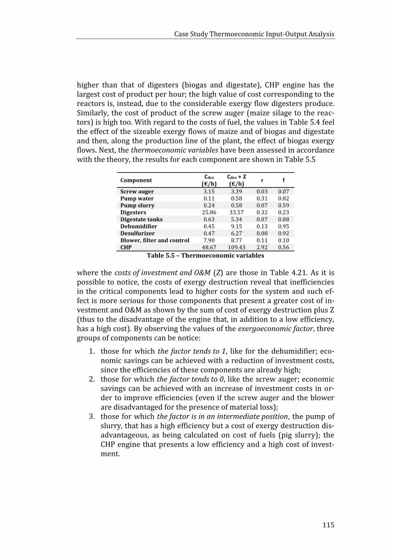
Case Study Thermoeconomic Input-Output Analysis
115
higher than that of digesters (biogas and digestate), CHP engine has the largest cost of product per hour; the high value of cost corresponding to the reactors is, instead, due to the considerable exergy flow digesters produce. Similarly, the cost of product of the screw auger (maize silage to the reac-tors) is high too. With regard to the costs of fuel, the values in Table 5.4 feel the effect of the sizeable exergy flows of maize and of biogas and digestate and then, along the production line of the plant, the effect of biogas exergy flows. Next, the thermoeconomic variables have been assessed in accordance with the theory, the results for each component are shown in Table 5.5
Component Cdes
(€/h) Cdes + Z (€/h)
r f
Screw auger 3.15 3.39 0.03 0.07 Pump water 0.11 0.58 0.31 0.82 Pump slurry 0.24 0.58 0.07 0.59 Digesters 25.86 33.57 0.32 0.23 Digestate tanks 0.63 5.34 0.07 0.88 Dehumidifier 0.45 9.15 0.13 0.95 Desulfurizer 0.47 6.27 0.08 0.92 Blower, filter and control 7.90 8.77 0.11 0.10 CHP 48.67 109.43 2.92 0.56
Table 5.5 – Thermoeconomic variables
where the costs of investment and O&M (Z) are those in Table 4.21. As it is possible to notice, the costs of exergy destruction reveal that inefficiencies in the critical components lead to higher costs for the system and such ef-fect is more serious for those components that present a greater cost of in-vestment and O&M as shown by the sum of cost of exergy destruction plus Z (thus to the disadvantage of the engine that, in addition to a low efficiency, has a high cost). By observing the values of the exergoeconomic factor, three groups of components can be notice:
1. those for which the factor tends to 1, like for the dehumidifier; eco-nomic savings can be achieved with a reduction of investment costs, since the efficiencies of these components are already high;
2. those for which the factor tends to 0, like the screw auger; economic savings can be achieved with an increase of investment costs in or-der to improve efficiencies (even if the screw auger and the blower are disadvantaged for the presence of material loss);
3. those for which the factor is in an intermediate position, the pump of slurry, that has a high efficiency but a cost of exergy destruction dis-advantageous, as being calculated on cost of fuels (pig slurry); the CHP engine that presents a low efficiency and a high cost of invest-ment.

5.
116
The analysis of the entire system has yielded an economic cost of products of 193.1 €/h composed for the 54% by fuel cost and for 46% by investment and O&M cost, since the cost of capital investment and operating and maintenance has been evaluated in the previous chapter to a value of 89.1 €/h.
5.2. Uncertainty evaluation
The relative uncertainty for each plant component exposed in Subpara-graph 4.5.1 has been used to characterize the probability distribution around the value of costs of each component. Hence, an exergoeconomic analysis has been performed once again for the existing case to highlight the range of values around results. Finally, a brief sensitivity analysis about as-sumptions for the definition of exergy destruction cost and for the uncer-tainty distribution has been carried out.
5.2.1. Exergoeconomic analysis with uncertainty evaluation
Monte Carlo simulations have been used to estimate the uncertainties in the exergoeconomic costs and variables in accordance with the theory offered in Chapter 3. The uncertainty has been introduced as ranges because in the interval in which data have been found there is not any value (even less a group of values) that occurs with a probability greater than that of the oth-ers. So, also the results are represented with uniform distributions. To eval-uate the propagation of uncertainties more than 1000 runs of Monte Carlo method have been required. In Figure 5.6 the results for the evaluation of the specific cost of product for each component are shown in €/toe (see Ap-pendix for results in €/kWh).
The results show that always cost values settle in the positions already dis-cussed but as soma intervals, not as a unique points. All the possible costs fall in the interval in accordance with the uncertainty of the inputs to the model (fuel and investment costs). The ranges are represented with a kind of box plot in which the whiskers reach the maximum and the minimum values of the interval. The variability around the mean value is up to 18% with a minimum to 12% for the pump of the pig slurry, anyway, it is be-tween the relative uncertainties of the input costs.

Case Study Thermoeconomic Input-Output Analysis
117
Figure 5.6 – Uncertainty ranges of the specific costs of product
The hourly costs of products are reported in Figure 5.7, the relative variabil-ity around the mean value is the same of the specific costs and this is true also for the costs of fuel and the cost of exergy destruction but not for the sum of cost of exergy destruction and investment cost, the relative cost dif-ference and the exergoeconomic factor.
0
200
400
600
800
1000
1200
1400
1600
1800
2000
Spe
cifi
c co
st o
f p
rod
uct
, cP
(€/t
oe
)
0
50
100
150
200
250
300
350
400
450
500
Spe
cifi
c co
st o
f p
rod
uct
, cP
(€/t
oe
)

5.
118
Figure 5.7 – Uncertainty ranges of the costs of product
In Figure 5.8 the costs per exergy unit of fuels for each component are dis-played.
Figure 5.8 – Uncertainty ranges of the specific costs of fuel
0
20
40
60
80
100
120
140
160
180
200C
ost
of
pro
du
ct, C
P(€
/h)
0
50
100
150
200
250
300
350
400
450
500
Spe
cifi
c co
st o
f fu
el,
cF
(€/t
oe
)

Case Study Thermoeconomic Input-Output Analysis
119
Even like intervals, the values show a growing trend along the production line of the system as the quality of the fuels increases from component to component; the fuel of screw auger, the maize silage, has a cost clearly higher than those of water and pig slurry. Then when these costs have been multiplied by the exergy flows that are inputs for the plant the hourly costs of fuel have been assessed with their uncertainty intervals as presented in Figure 5.9. That is why the digesters have the highest costs (even if not the largest dispersion own of blower and CHP engine): the exergy flow of the feedstock mix is the highest.
Figure 5.9 – Uncertainty ranges of the costs of fuel
The costs of exergy destruction have been estimated with their uncertainty intervals to the value presented in Figure 5.10. The largest values are those of the components in which the exergy destructions are the highest, first of all CHP engine and the digesters (with a relative uncertainty around the mean value of 18% and 17% respectively) and then the blower and the screw auger (18% and 17% of variability). By adding to these costs, those of capital investment and operating and maintenance per hour shown in Table 4.21 accompanied with uncertainties reported in Table 4.23, the values of the costs of exergy destruction plus Z have been estimated. Observing Figure 5.11 it is possible to notice the influence of the costs of the components es-pecially for the CHP engine and for the components used in the treatments of the biogas after the digestion.
0
20
40
60
80
100
120
140
160
180
Co
st o
f fu
el,
CF
(€/h
)

5.
120
Figure 5.10 – Uncertainty ranges of the costs of exergy destruction
The sum of these costs with different uncertainties also has an effect on the uncertainty of the total variables: intervals are not exactly symmetric, the uncertainties increase for various components, up to 33% of dispersion for the cost values of the dehumidifier since it has been considered the most
0
10
20
30
40
50
60
70C
ost
of
exe
rgy
de
stru
ctio
n, C
de
s(€
/h)
0
1
2
3
4
5
6
7
8
9
10
Co
st o
f ex
erg
y d
est
ruct
ion
, Cd
es
(€/h
)

Case Study Thermoeconomic Input-Output Analysis
121
expensive component among those of biogas treatment; for the digesters, instead, the variability around the mean value decrease to the minimum of 14% amongst all the components.
Figure 5.11 – Uncertainty ranges of the costs of exergy destruction
and of investment and O&M
0
20
40
60
80
100
120
140
Co
st o
f ex
erg
y d
est
ruct
ion
plu
s ca
pit
al
inve
stm
en
t an
d O
&M
, Cd
es+Z
(€
/h)
0
2
4
6
8
10
12
14
Co
st o
f ex
erg
y d
est
ruct
ion
plu
s ca
pit
al
inve
stm
en
t an
d O
&M
, Cd
es+
Z (€
/h)

5.
122
The relative cost difference and the exergoeconomic factor have been esti-mated too, their values intervals are shown in Figure 5.12 and Figure 5.13.
Figure 5.12 – Uncertainty ranges of the relative cost difference
0,00
0,50
1,00
1,50
2,00
2,50
3,00
3,50
4,00
Re
lati
ve c
ost
dif
fere
nce
, r
0,00
0,05
0,10
0,15
0,20
0,25
0,30
0,35
0,40
0,45
Re
lati
ve c
ost
dif
fere
nce
, r

Case Study Thermoeconomic Input-Output Analysis
123
The effect of uncertainties propagations has been ascertained in each com-ponent for the relative cost difference:
the screw auger, the digesters and the blower present a relative un-certainty below 10%, up to 2% for the screw auger;
the pumps, the digestate tanks and the CHP engine have an uncer-tainty between 14% and 33%;
the dehumidifier and the desulfurizer present a high uncertainty over 33% and up to 50% for the dehumidifier, compensated by the fact that the values in question are very low.
Even for relative cost difference and exergoeconomic factor intervals are not symmetric albeit slightly.
Figure 5.13 – Uncertainty ranges of the exergoeconomic factor
The effect of the propagation of different uncertainties for the exergoeco-nomic factor has yielded a relatively low dispersion (below 14%) for all components except for the digesters which present a relative uncertainty up to 24% and further for the screw auger and the blower which have rela-tive uncertainties up to 36% and 46% respectively, even here compensated by the fact that the values in question are very low.
The cost of product of the entire system has been estimated to the median value of 192.6 €/h with a relative uncertainty of 16%.
0,00
0,10
0,20
0,30
0,40
0,50
0,60
0,70
0,80
0,90
1,00
Exe
rgo
eco
no
mic
fact
or,
f

5.
124
Bearing in mind all these considerations, it has been possible to evaluate the needed steps to enhance cost-effectiveness of the entire plant. The main component that needs more attention and interest of development is, of course, the engine both for its high cost of investment and operating and maintenance and for that of exergy destruction (up to 1014459 € per year) even if it is difficult to imagine that the research to reduce inefficiencies would result in a reduction of engine cost. Next an accurate focus would be directed towards the digesters and the components for the biogas treatment. Also the information given by the relative cost difference underlines these priorities. To reduce the costs of components for biogas treatment, even at the expense of a little loss of efficiency, and to minimize the material losses of maize and biogas from the screw auger and the biogas treatment phase is necessary to improve cost-effectiveness. As well as to reduce the irreversi-bilities in the processes occurring within the digesters and the CHP engine is needed.
5.2.2. Uncertainty due to model assumptions
The uncertainty linked to the assumptions of the model has been studied re-garding the definition of the cost of exergy destruction that, as seen, is a very important thermoeconomic variable. On the basis of theory in Subpara-graph 2.1.2 the cost of exergy destruction can be defined as the cost rate of the additional fuel that must be supplied to the component in question to cover the rate of exergy destruction or as the monetary loss associated with the loss of product. This way, it is a crucial variable of the thermoeconomic models and its definition characterizes the intrinsic uncertainty of the mod-el itself. Such an uncertainty is represented in Figure 5.14 as the possible range of the values that the costs of exergy destruction can take for each component.
Neither of the two assumptions used to define the cost is strictly satisfied and these definitions are just approximations of the average costs rate asso-ciated with exergy destruction. The use of the specific cost of fuel or of product respectively gives a lower or a higher estimate with the actual ex-ergy destruction cost being somewhere between the two within the ranges. As it is observable, the change in the assumption is not significant for vari-ous components except for the two in which material loss occur and the other two in which inefficiencies are relevant. In both cases the process irre-versibilities affect the value of the exergy destruction and accordingly the ranges of the cost of exergy destruction so much so that the intervals are as wider as the exergy destruction in the component in question is higher. For

Case Study Thermoeconomic Input-Output Analysis
125
the CHP engine, in which the inefficiencies are the largest, the variability around the mean value is high to 39%, for the digesters is equal to 11%, for all the other components is under 5%.
Figure 5.14 – Uncertainty ranges due to the different definitions
of exergetic cost of exergy destruction
0
50
100
150
200
250
300
350
400
450
Co
st o
f ex
erg
y d
est
ruct
ion
, Cex
e,d
es
(ko
e/h
)
0
5
10
15
20
25
30
35
40
Co
st o
f ex
erg
y d
est
ruct
ion
, Cex
e,d
es
(ko
e/h
)
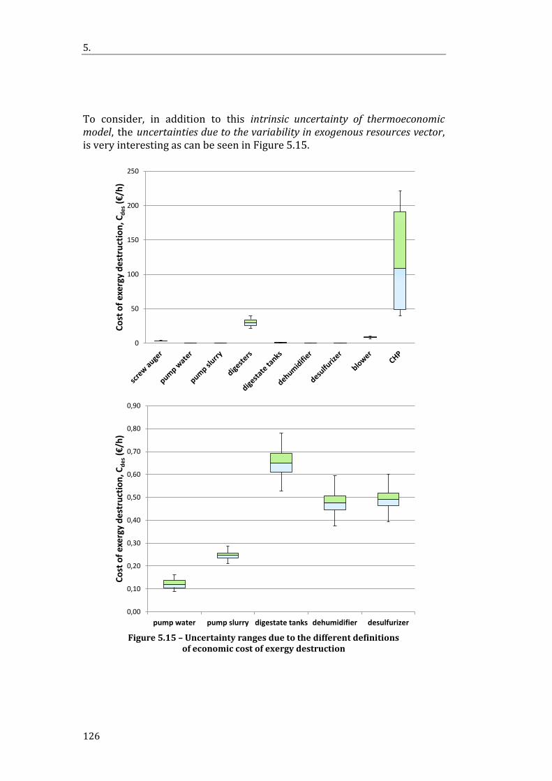
5.
126
To consider, in addition to this intrinsic uncertainty of thermoeconomic model, the uncertainties due to the variability in exogenous resources vector, is very interesting as can be seen in Figure 5.15.
Figure 5.15 – Uncertainty ranges due to the different definitions
of economic cost of exergy destruction
0
50
100
150
200
250
Co
st o
f ex
erg
y d
est
ruct
ion
, Cd
es
(€/h
)
0,00
0,10
0,20
0,30
0,40
0,50
0,60
0,70
0,80
0,90
pump water pump slurry digestate tanks dehumidifier desulfurizer
Co
st o
f ex
erg
y d
est
ruct
ion
, Cd
es
(€/h
)

Case Study Thermoeconomic Input-Output Analysis
127
In fact, the CHP engine show a very high variability (up to 86%) so that the information provided is insignificant as all values between 40 and 222 €/h could be the actual cost of exergy destruction for that component. Even for the digesters the uncertainty is high but lesser (up to 33%), for the other components is under 32%. Hence, when efficiency is low and consequently the exergy destruction is large, to know the value of exergy destruction cost rate becomes very hard.
Another important aspect analyzed is the arbitrary assumption about the uncertainty distribution. Up to now the only distribution analyzed has been the uniform distribution (since no information has led to think that, for ex-ample, there is a greater probability that the values of the results fall in the middle of the intervals) but, some academics [7] suggest the use of the Gaussian distribution for the uncertainty evaluation. Through Monte Carlo simulations it is possible to simulate this distribution characterizing the dispersion of a parameter with a mean value and a standard deviation. Whit the relative uncertainty available in Table 4.23, the percentage of the total uncertainty has been used to generate the standard deviation and the cen-tral value of the cost has been utilized as mean value. Figure 5.16 presents a comparison between the calculation of the cost of products with a uniform and a normal distribution.
Figure 5.16 – Uncertainty ranges due to the different distributions:
uniform (on the left) and Gaussian (on the right)
In a simply way, the Gaussian distribution, by taking into account also the costs that have a very low probability to happen, broadens the uncertainty ranges. These considerations are valid for an analysis ex post the construc-tion of the plant with the little information available; in a context ex ante plant building all the possible costs are known by the designer and so, when there are uncertainties, the real distributions are known too.
0
20
40
60
80
100
120
140
160
180
200
CHP
Co
st o
f p
rod
uct
, CP
(€/h
)
0
20
40
60
80
100
120
140
160
180
200
CHP
Co
st o
f p
rod
uct
, CP
(€/h
)

5.
128
5.3. Design optimization
At the conclusion of the work, a design optimization of the system in ques-tion has been performed. The aim of such a study is the research of the op-timum mix between the two feedstocks of the plant, the maize silage and the pig slurry, that guarantees the economic optimum, with the lowest costs and the largest profits and the thermodynamic optimum, through a thermoeco-nomic Input-Output analysis, with the lowest resources consumption. Thus, the chosen parameter for the optimization is the mass fraction of maize, the only input of the plant considered together with the slurry. The search of the optimum would permit the plant to work in the most efficient way and with the lowest cost, for instance, with the lowest use of maize as this fuel is more expensive than the slurry. The optimization has been carried out with the limit of the constant plant principal output: in each configuration the electrical power produced is constant to 995 kW as the thermal power to 1076 kW. The 12 configurations considered cover all the possible feedstock mix from 0% of maize (equal to 100% of slurry) to 100% of maize (0% of slurry). In the first configuration there are not costs of maize, screw auger and pump of water and exergy flows regarding these components are equal to zero. In the last configuration there are not costs of slurry and pump of slurry, so, exergy flows at the turn of this component are equal to zero.
5.3.1. Economic considerations
The economic analysis shown in the previous paragraphs has been reap-plied for all the configurations, the cost analysis has yielded the results pre-sented in Figure 5.17 varying percentage of maize introduced in the plant. For the first five configurations the capital investment is larger than that of the last seven configurations because of the higher costs for the digesters and the digestate tanks. In fact, in the first five configurations, as the maize silage utilized is modest, a lot of slurry has to be used to obtain the constant power output. This results in a greater volume of the feedstock introduced in the reactors or rather in an increase of the number of reactors for the plant. In the configuration with 100% slurry, 829 t/d of pig slurry are required, so the feedstock volume must be divided into 6 digesters and the produced di-gestate in the same number of tanks. For the configuration with 5% of maize silage, the number of reactors has been estimated equal to 4, 3 for those with 15%, 25% and 35% of maize, while from 45% to 100% of maize 2 reactors are sufficient. The costs analysis show that there is not a predom-inant configuration which permits large reduction of costs, excluding the

Case Study Thermoeconomic Input-Output Analysis
129
first five configuration with a total cost from 223 to 198 €/h, the configura-tions from 45% up to 100% of maize input are equivalent with a total cost of 193 €/h.
Figure 5.17 – Cost composition
Fig
ure
5.1
7 –
Co
st c
om
po
siti
on
0
50
10
0
15
0
20
0
25
0
0%
5%
15
%2
5%
35
%4
5%
55
%6
5%
75
%8
5%
95
%1
00
%
Total cost of product, CP,tot(€/h)
y mai
ze
C_s
lurr
y
C_m
aiz
e
Z_C
HP
Z_b
low
er
Z_d
esu
lfu
rize
r
Z_d
eh
um
idif
ier
Z_d
iges
tate
tan
ks
Z_d
iges
ters
Z_p
um
p w
ate
r
Z_p
um
p s
lurr
y
Z_sc
rew
au
ger

5.
130
In order to find the economic optimum, also a profitability analysis has been performed for each configuration and results are reported in Table 5.6.
ymaize NPV (€)
PBP (y)
IRR (%)
LCOE (€/kWh)
0% 1262831 15 8 0.212 5% 1724098 13 10 0.203 15% 1956274 12 11 0.199 25% 1956622 12 11 0.199 35% 2636251 10 12 0.199 45% 2868625 10 13 0.194 55% 2871186 10 13 0.194 65% 2869236 10 13 0.194 75% 2869561 10 13 0.194 85% 2869942 10 13 0.194 95% 2870510 10 13 0.194 100% 2871727 10 13 0.194
Table 5.6 – Profitability indicators and LCOE
Even this analysis confirm that from 45% of maize input all configurations allow to reach the highest profits. For the first five configurations the incen-tives considered have been estimated to the lower value of 0.209 €/kWh since the premium for the cogeneration cannot be given for the failed pri-mary energy saving of 10% for these plants. The configuration with 55% of maize (the existing case) and that with 100% of maize input are those for which the net present value is higher albeit slightly. The levelized cost of electricity has been also evaluated as displayed in Table 5.6 and the results conform to what already seen.
5.3.2. Thermoeconomic considerations
With a thermoeconomic analysis of all the plant as a whole for each configu-ration has been assessed the trend of the exergy destruction as shown in Figure 5.18. No central information can be inferred from such a flat trend except that of the main value, round 295 koe/h (about 3430 kW) equal to about 4 times the net electrical power of the plant. Figure 5.19 presents the trend of the exergetic efficiency and shows that the configuration with the highest efficiency is that with 0% of maize and then the trend decreases. The trends of exergetic cost of product and economic cost of product with the associated uncertainties intervals have been calculated and exposed in Fig-ure 5.20. Both present the lowest costs with increasing the amount of maize introduced in the plant. The exergetic cost tends to the value of 600 koe/h (about 7000 kW). The ranges of the economic costs have been evaluated as explained in the previous paragraphs to obtain a relative uncertainty not

Case Study Thermoeconomic Input-Output Analysis
131
bigger than 17% (for the configurations with 95% and 100% of maize in-put).
Figure 5.18 – Exergy destructions
Figure 5.19 – Exergetic efficiencies
0
50
100
150
200
250
300
350
0% 10% 20% 30% 40% 50% 60% 70% 80% 90% 100%
Exe
rgy
de
stru
ctio
n, E
de
s(k
oe
/h)
ymaize
0%
10%
20%
30%
40%
50%
60%
70%
80%
0% 10% 20% 30% 40% 50% 60% 70% 80% 90% 100%
Exe
rget
ic e
ffic
ien
cy, η
exe
ymaize

5.
132
Figure 5.20 – Exergetic and economic costs of product
At last, the values of the two components of the economic cost of product have been estimated and presented in Figure 5.21: the cost of fuel and of in-vestment and maintenance. The cost of product is given by the sum of these two.
0
200
400
600
800
1000
1200
0% 10% 20% 30% 40% 50% 60% 70% 80% 90% 100%
Co
st o
f p
rod
uct
, Cex
e,P
(ko
e/h
)
ymaize
0
50
100
150
200
250
300
0% 5% 15% 25% 35% 45% 55% 65% 75% 85% 95% 100%
Co
st o
f p
rod
uct
, CP
(€/h
)
ymaize

Case Study Thermoeconomic Input-Output Analysis
133
Figure 5.21 – Costs of capital investment and O&M and of fuel
So, it is possible to conclude that all the configuration from 45% of maize input upward are equivalent for the minimization of the costs both exerget-ic and economic. Even economic analysis confirm this conclusion, neverthe-less, with a comparison with Figure 5.19 an intermediate configuration (the existing case 55% of maize input) is preferable not to reduce too much the
0
50
100
150
200
250
300
0% 5% 15% 25% 35% 45% 55% 65% 75% 85% 95% 100%
Co
st o
f ca
pit
al in
vest
me
nt
and
O&
M, Z
(€
/h)
ymaize
0
50
100
150
200
250
300
0% 5% 15% 25% 35% 45% 55% 65% 75% 85% 95% 100%
Co
st o
f fu
el,
CF
(€/h
)
ymaize

5.
134
efficiency of the system. Moreover, the choice of a configuration with 55% of maize input instead of 100%, for instance, allows the use of a greater amount of slurry. The energy valorization of such an agricultural byproduct is important also to avoid an uncontrolled release into the atmosphere of me-thane.
135
6. Conclusions
This thesis presents a method for the uncertainty evaluation and the uncer-tainty propagation assessment in thermoeconomic Input-Output analysis. The context in question is that of the valorisation and the description of the nat-ural, exergy resources necessary in production chains to yield products. All the available instruments, the exergetic, economic and statistical analyses have been utilized to elaborate the methodology.
The concept of available and destroyed energy, together with the economic concept of cost have been used in the thermoeconomic analysis to estimate the cost of the product of a system starting from the system dataset and ac-cessible information. Since each type of data presents some uncertainty, the main statistical instruments to describe it have been provided. The problem to study uncertainty propagation has been solved through the application of various Monte Carlo simulations in order to evaluate the uncertainty in the results of the Input-Output analysis, the costs and the thermoeconomic var-iables. Monte Carlo technique is an approach very fast and reliable whenev-er to handle a huge amount of data is possible.
Also thanks to the application of the method in a case study, it has been pos-sible to verify how thermoeconomic analysis is of central importance for the characterization of the resources needed to produce goods. However, it must be accompanied by a consistent uncertainty analysis to assess the var-iability linked to results and to perform a critical evaluation of the achieved information. In fact, the assumptions about the model affect the validity of the results, so that they need to be assessed case by case carefully remem-bering that there is more dispersion where the exergetic inefficiency is high-er. Systems in which the exergy destruction is larger, and in which the ex-ergetic efficiency is lower, are those on which it is necessary to invest to re-duce irreversibilities.
The uncertainty evaluation can be useful also in the problems of ther-moeconomic optimization since the characterization of intervals instead of fixed point may lead to different conclusions in the cost minimization pro-cess.
It is important to underline that, even if in this work the application of the methodology based on Monte Carlo simulations has been applied at that part of the matrixes arrangement of Input-Output analysis identified as economic resources vector, the formalisation of the method for the analysis is general. In principle, uncertainty affects every kind of data, thus variabil-ity and dispersion can characterize the exogenous resources and the final

136
demand vectors up to spread in the Leontief inverse matrix. This way, the described methodology for Input-Output analysis may be applied in differ-ent fields as well as that of Life Cycle Assessment, for the supply chains analysis, thanks to its versatility. In effect, once established the uncertain-ties in input data, by Monte Carlo simulations, the uncertainties that have reached the output results may be estimate, so that an accurate data gather-ing phase and some good computing capabilities are the key points for a suc-cessful implementation of the method.

137
References
[1] D. C. Montgomery, G. C. Runger, and N. F. Hubele, Engineering Statistics. Jhon Wiley & Sons, Inc., 2004.
[2] P. F. Chapman, “Energy costs: a review of methods,” Energy Policy, pp. 92–103, 1974.
[3] B. R. Bakshi, T. G. Gutowski, and D. P. Sekulic, Thermodynamics and the destruction of resources. Cambridge: Cambridge University Press, 2011.
[4] A. Bejan, M. Moran, and G. Tsatsaronis, Thermal design and optimization. New York: John Wiley & Sons, Inc., 1996.
[5] C. T. Hendrickson, L. B. Lave, and H. S. Matthews, Environmental Life Cycle Assessment of Goods and Services: An Input-Output Approach. Washington: Resources for the Future, 2006.
[6] M. Goedkoop, A. De Schryver, M. Oele, S. Durksz, and D. de Roest, Introduction to LCA with SimaPro 7. San Francisco: PRé, 2010.
[7] M. Lenzen, “Errors in Conventional and Input-Output based Life Cycle inventories,” J. Ind. Ecol., vol. 4, 2001.
[8] I. Dincer and M. A. Rosen, “Exergy: Energy, Environment and Sustainable Development.” Elsevier, 2013.
[9] M. J. Moran and H. N. Shapiro, Fundamentals of engineering thermodynamics. New York: Wiley, 2006.
[10] S. J. de Oliveira, Exergy Production, Cost and Renewability. London: Green Energy and Technology, 2013.
[11] J. Szargut, “Anthropogenic and natural exergy losses (exergy balance of the Earth’s surface and atmosphere),” Energy, vol. 28, pp. 1047–1054, 2002.
[12] G. Wall, “Exergy - a useful concept within resources accounting,” Gotenborg, 1977.
[13] G. Lozza, Turbine a gas e cicli combinati. Bologna: Progetto Leonardo, 2006.

138
[14] J. Deng, R. Wang, J. Wu, G. Han, D. Wu, and S. Li, “Exergy cost analysis of a micro-trigeneration system based on the structural theory of thermoeconomics,” Energy, vol. 33, no. 9, pp. 1417–1426, Sep. 2008.
[15] U. Desideri, G. Manfrida, and E. Sciubba, ECOS 2012 The 25th International Conference on Efficiency, Cost, Optimization and Simulation of Energy Conversion Systems and Processes (Perugia, June 26th-June 29th, 2012). Firenze: Firenze University Press, 2012.
[16] R. E. Miller and P. D. Blair, Input-Output Analysis Functions and Extensions. Cambridge, 2009.
[17] W. Leontief, Input-Output Economics. New York: Oxford University Press, 1986.
[18] S. Uson and A. Valero, Thermoeconomic Diagnosis of Energy Systems. Zaragoza, Prensas Universitaria de, 2010.
[19] E. Querol, B. Gonzalez-Regueral, and J. L. Perez-Benedito, Practical Approach to Exergy and Thermoeconomic Analyses of Industrial Processes. London: Springer London, 2013.
[20] C. Torres Cuadra and A. Valero Capilla, Thermoeconomic Analysis. Madrid, 2005.
[21] UNI, “Vocabolario Internazionale di Metrologia.” Milano, 2010.
[22] F. S. Levin, An Introduction to Quantum Theory. Cambridge: Cambridge University Press, 2002.
[23] A. S. Morris, Measurement and Instrumentation Principles. Oxford: Butterworth-Heinemann, 2001.
[24] D. G. Cacuci, I. M. Navon, and M. Ionescu-Bujor, Sensitivity and Uncertainty Analysis. Boca Raton: Chapman & Hall/CRC, 2005.
[25] R. Heijungs and S. Suh, The Computational Structure of Life Cycle Assessment. Springer Science+Business Media Dordrecht, 2002.
[26] P. Balestra, La derivation matricielle Technique et resultats pour economistes. Paris: Sirey, 1976.
[27] C. Robert and G. Casella, Monte Carlo Statistical Methods. New York: Springer, 2010.

139
[28] N. T. Thomopoulos, Essentials of Monte Carlo Simulation. Springer, 2013.
[29] R. E. Quandt, “On the solution of probabilistic Leontief systems,” Nav. Res. Logist. Q., vol. 6, pp. 295–305, 1959.
[30] O. J. Hanssen and O. A. Asbjørnsen, “Statistical properties of emission data in life cycle assessments,” J. Clean. Prod., vol. 4, pp. 149–157, 1996.
[31] P. S. M. Kop Jansen, “Analysis of multipliers in stochastic input-output systems,” Reg. Sci. Urban Econ., vol. 24, pp. 55–74, 1994.
[32] C. W. Bullard and A. V. Sebald, “Monte Carlo Sensitivity Analysis of Input/Output Models,” Rev. Econ. Stat., vol. 70, p. 5, 1988.
[33] C. W. Bullard, D. L. Putnam, A. V. Sebald, and D. L. Amado, “Stochastic Analysis of Uncertainty in a U.S. Input/Output Model,” University of Illinois, Urbana, 1976.
[34] F. C. Knopf, Modeling, Analysis and Optimization of Process and Energy Systems. Hoboken: Jhon Wiley & Sons, Inc., 2012.
[35] F. Reale, R. Stolica, M. Gaeta, M. Ferri, M. Sarnataro, and V. Vitale, “Analisi e stima quantitativa della potenzialità di produzione energetica da biomassa digeribile a livello regionale . Studio e sviluppo di un modello per unità energetiche Parte 4 - Studio di un modello energetico,” 2009.
[36] J. Bacenetti, M. Fiala, S. Gonzalez-Garcia, and M. Negri, “Anaerobic digestion of different feedstocks: Impact on energetic and environmental balances of biogas process,” Sci. Total Environ., p. 12, 2013.
[37] F. Fantozzi and C. Buratti, “Biogas production from different substrates in an experimental Continuously Stirred Tank Reactor anaerobic digester,” Bioresour. Technol, vol. 100, 2009.
[38] M. Fiala, Energia da biomasse agricole. Santarcangelo di Romagna: Maggioli Editore, 2012.
[39] D. Dressler, A. Loewen, and M. Nelles, “Life cycle assessment of the supply and use of bioenergy: impact of regional factors on biogas production,” Int J Life Cycle Assess, vol. 17, 2012.
[40] S. C. Capareda, Introduction to Biomass Energy Conversions. Boca Raton: CRC Press, 2014.

140
[41] A. Campi, E. Macchi, G. Bilato, V. Garavaglia, and G. Valenti, “Il progetto Agrengest,” AEIT, vol. 3, p. 22, 2009.
[42] J. Bacenetti and M. Negri, “Pulire il biogas,” Macch. Agric., vol. maggio, p. 3, 2013.
[43] M. Giommi, “Impianto per la produzione di energia elettrica di potenza nominale di 998 kWel mediante l’utilizzo di biogas prodotto dalla digestione anaerobica di prodotti agricoli vegetali,” Solenergia s.r.l., Montefelcino, 2012.
[44] J. Bacenetti, A. Cantore, P. Cantarella, M. Fiala, and M. Negri, “A detailed monitoring of a anaerobic digestion plant in northern Italy,” Environ. Eng. Manag. J., vol. 12, p. 4, 2013.
[45] Autorità per l’energia elettrica e il gas, “Condizioni per il riconoscimento della produzione combinata di energia elettrica e calore come cogenerazione ai sensi dell’articolo 2, comma 8, del decreto legislativo 16 marzo 1999, n.79.” p. 13, 2002.
[46] Autorità per l’energia elettrica e il gas, “Aggiornamento dei parametri di riferimento per il riconoscimento della produzione combinata di energia elettrica e calore come cogenerazione ai sensi dell’articolo 2, comma 8, del decreto legislativo 16 marzo 1999, n.79.” 2005.
[47] T. J. Kotas, “The Exergy Method of Thermal Plant Analysis.” Krieger Publishing Company, Malabar, 1996.
[48] B. G. A. Visconti, “Progetto per la costruzione di un impianto per la produzione di energia elettrica da fonti rinnovabili,” Azienda Agricola Edoardo Visconti di Modrone, Torre Beretti e Castellaro, 2011.
[49] M. S. Peters, K. D. Timmerhaus, and R. E. West, Plant Design and Economics for Chemical Engineers. McGraw-Hill Higher Education, 2003.
[50] C. A., “Casalvolone - Imminente inaugurazione della centrale a biogas per la produzione di energia elettrica,” Vercelli Oggi.it, Piemonte Oggi Srl, Vercelli, p. 1, 09-Mar-2011.
[51] A. Bruno, Fonti rinnovabili Autorizzazioni, connessioni, incentivi e fiscalità della produzione elettrica. Cesano Boscone: Edizioni Ambiente, 2012.

141
Appendixes
Exergy cost analysis, existing case
Component Edes
(kW) ηexe
Screw auger 193 97% Pump water 14 95% Pump slurry 17 97%
Digesters 1434 80% Digestate tanks 25 99%
Dehumidifier 18 99% Desulfurizer 17 99%
Blower, filter and control 262 91% CHP 1451 44%
Exergy destruction and efficiencies of plant components
Component cexe,P Cexe,P (kW)
cexe,F Cexe,des (kW)
r
Screw auger 1.06 6642 1.03 198 0.03 Pump water 1.22 295 1.15 16 0.06 Pump slurry 1.11 683 1.08 18 0.03
Digesters 1.37 7968 1.10 1579 0.25 Digestate tanks 1.40 4134 1.39 35 0.01
Dehumidifier 1.39 3966 1.38 25 0.01 Desulfurizer 1.41 4005 1.40 24 0.01
Blower, filter and control 1.55 3986 1.41 369 0.10 CHP 3.57 3991 1.55 2254 1.30
Costs of products, fuels, exergy destruction and relative cost difference

142
Uncertainty evaluation, existing case
Uncertainty ranges of the specific costs of product
Uncertainty ranges of the specific costs of fuel
0,00
0,02
0,04
0,06
0,08
0,10
0,12
0,14
0,16
0,18
Spe
cifi
c co
st o
f p
rod
uct
, cP
(€/k
Wh
)
0,000
0,005
0,010
0,015
0,020
0,025
0,030
0,035
0,040
0,045
Spe
cifi
c co
st o
f fu
el,
cF
(€/k
Wh
)