political polarization and income inequality · pdf filecomparative political economy has...
TRANSCRIPT

Political Polarization and Income Inequality
Nolan McCarty
Princeton University
Keith T. Poole University of Houston
Howard Rosenthal
Princeton University and Russell Sage Foundation
27 January 2003
Abstract
Politics in the United States can now be characterized as an ideologically polarized two-party system. The economy features increased income inequality. While the literature on comparative political economy has focused on the links between economic inequality and political conflict, the relationship between these trends in the United States remains essentially unexplored. Using National Election Study data from 1952 to 2000, we explore the relationship between income and voter partisan self-identification. We find that partisanship has become more stratified by income. We argue that this trend is largely the consequence of polarization of the parties on economic issues and the development of a two-party system in the South. The trend is much less a reflection of increased economic inequality. The partisanship results replicate for presidential vote choice. We also find that the two-party system has adjusted to remain competitive in spite of the large increases in real income on the last half of the twentieth century. If voters in 2000 were voting as if real average income were only that of 1960, partisanship would have swung strongly in the Republicans favor.
For Richard McKelvey, in memoriam. This research was conducted as part of the Russell Sage Foundation’s Inequality Project at Princeton. Previous versions were presented in seminars or conferences at Harvard, NYU, Princeton, Russell Sage Foundation, Salerno, Stanford and Washington University. We thank participants for their comments. Correspondence to: Nolan McCarty, Woodrow Wilson School, Princeton University, Princeton, NJ. 08544, [email protected]

1
1. Introduction
The decade of the 1970s marked many fundamental changes in the structure of
American society. In particular, America witnessed almost parallel transformations of
both its economic structure and the nature of its political conflict.
The fundamental economic transformation has led to greater economic inequality
with incomes at the lowest levels stagnant or declining while individuals at the top have
prospered. The Gini coefficient of family income, a standard measure of inequality, has
risen by more than 20% since its low point in 1968 (U.S. Census Bureau, 2002).1 A
remarkable fact about this trend is that it began after a long period of increasing equality.2
Economists and sociologists have allocated tremendous effort into discovering the root
causes of this transformation. Numerous hypotheses have been put forward including
greater trade liberalization, increased levels of immigration, declining rates of trade
unionization, the fall in the real minimum wage, technological change increasing the
returns to education, and the increased rates of family dissolution and female headed
households.3
Within the political realm, the 1970s were also transformative. The decade
witnessed both a partisan realignment in the Southern states and increased polarization in
the policy positions of Democrats and Republicans. As we, together and separately, have
documented in previous work, the bipartisan consensus among elites (Congress in
particular) about economic issues that characterized the 1960s gave way to the deep
ideological divisions of the 1990s (Poole and Rosenthal, 1984, Poole and Rosenthal
1997, McCarty, Poole, and Rosenthal 1997). Furthermore, we have found that previously
orthogonal conflicts have disappeared or been incorporated into the conflicts over

2
economic liberalism and conservatism. Most importantly, issues linked to race are now
largely expressed as part of the main ideological division over redistribution.
Remarkably, the trends of economic inequality and elite political polarization
have moved almost in tandem for the past half-century. Figure 1 plots the levels of
inequality as measured by the Gini coefficient along with a measure of political
polarization which is the average distance between Democratic and Republican members
of Congress in DW-NOMINATE scores.4 The polarization measure reflects the average
difference between the parties on a liberal-conservative scale. The proximity of these
trends is uncanny. In fact, inequality and polarization start increasing at approximately
the same time.
Figure 1
Income Inequality and Political Polarization
0.55
0.60
0.65
0.70
0.75
0.80
0.85
0.90
0.95
1947 1951 1955 1959 1963 1967 1971 1975 1979 1983 1987 1991 1995 1999
Pola
rizat
ion
Inde
x
0.330
0.345
0.360
0.375
0.390
0.405
0.420
0.435
0.450
Gin
i Ind
ex
House Polarization Index
Gini Index
r = .91

3
There is similar evidence that partisan affiliation in the mass public is increasingly
polarized in terms of liberal-conservative views. Green, Palmquist, and Schickler (2002)
report that the difference between the “percentage of Republicans who call themselves
conservatives” and the “percentage of Democrats who call themselves conservatives” has
doubled between 1972 and 1996, moving from 25% to 50%.5
While it makes intuitive sense that economic inequality may breed political
conflict (or even the converse), almost no work has been done to explain such a
conjunction within the context of American politics.6 Perhaps one reason for this dearth
of interest is that traditionally income or wealth has not been seen as a reliable predictor
of political beliefs and partisanship in the mass public, especially in comparison to other
cleavages such as race and region or in comparison to other democracies.7 If political
conflict does not have an income basis, it makes little sense that changes in economic
inequality would disturb existing patterns of political conflict.
However, the fact that American politics has not always been organized as a
contest of the haves and have-nots does not mean that it will always be that way. If
income and wealth are distributed in a fairly equitable way, little is to be gained for
politicians to organize politics around non-existent conflicts. In this context, it is
interesting that much of our empirical knowledge about the nature of American political
attitudes and partisanship is drawn from surveys conducted during an era of relatively
equal economic outcomes.
Partisanship (as measured by the National Election Study) was, in fact, only
weakly related to income in the period following World War II. In the presidential
election years of 1956 and 1960, respondents from the highest income quintile were

4
hardly more likely to identify as a Republican than were respondents from the lowest
quintile. In contrast, in the two presidential election years of the 1990s, respondents in
the highest quintile were more than twice as likely to identify as a Republican than were
those in the lowest.
We summarize how partisanship has acquired an income basis through an index
of party-income stratification. Our index is simply the proportion of Republican
identifiers (strong and weak) in the top income quintile divided by the proportion of
Republican identifiers in the bottom quintile.8 As seen in figure 2, the stratification of
partisanship by income has steadily increased over the past 40 years, leading to an
increasing rich-poor cleavage between the parties.
In figure 2, we have also plotted stratification for the presidential vote. Here we
compute the ratio of the fraction of Republican voters among voters for the two major
parties in the top quintile to the same fraction in the bottom quintile. The upward trend,
in stratification is also evident for the presidential vote.
Of course, the simple bivariate relationship between stratification and income
does not show that the party system is increasingly organized along income lines. These
results could be due to changing income characteristics of party constituencies based on
other cleavages. While not denying this claim (in fact, we present some evidence for it
below), we insist that regardless of the mechanism that created the stratification of
partisanship by income, the mere fact that there are substantial income differences across
the constituencies of the two parties has important implications for political conflict. As
parties are generally presumed to represent the interests of their base constituencies, the
income stratification should contribute to the parties pursuing very different economic

5
policies. Moreover, public policy may be shifting away from policies that are based on
self-identified racial, ethnic, or gender characteristics. The shift could be to policies,
such as preferred access to higher education for children from poor homes or earned
income tax credits, which are income or wealth based. Such a shift would reinforce
interest in studying the income stratification of partisan identification.
Figure 2
Notes: Stratification of partisanship is calculated in each NES survey from 1952 to 2000. Stratification of presidential votes is calculated only in presidential election year surveys.
To explore the relationship between the economic and political transformations
that we have discussed, the rest of the paper attempts to provide some explanations for
the causes of the increased party-income stratification. We focus on partisan
identification because it is one item from the National Election Study that is present in
every study from 1952 to 2000. Moreover, unlike presidential vote intention or choice, it
is less influenced by election-specific factors, such as the perceived extremity of the
candidates or their “charisma”. We are able, however, to show that our results for

6
partisanship largely replicate for presidential vote choice, although, as is to be expected,
the results are somewhat noisier.
Logically, there are four non-mutually exclusive reasons why stratification might
have increased. First, there could be a response effect. There can be a temporal increase
in the coefficient for income in our model of partisanship. Below we argue that this is
consistent with party polarization on economic policy issues. Second, there may be an
inequality effect. Increased inequality might have made low income groups relatively
poorer and high-income groups richer so that with even a small, constant response effect
stratification would increase. Third, increased stratification might be a result of a change
in the joint distribution of other demographic characteristics and income. Pro-
Democratic groups may have gotten poorer while pro-Republican groups got richer. For
example, African-American partisanship may have remained unchanged but the relative
poverty of African-Americans may have increased. Finally, groups with high incomes
may have moved toward the Republicans while poorer groups moved toward the
Democrats. For example, the relative poverty of African-Americans may have remained
unchanged but their propensity for Democratic identification increased.
To quantify each of these effects, we estimate a model of party identification and
its relationship to income and other characteristics. We then use the estimates of this
model as well as data about the changing distribution of income to calculate the level of
party-income stratification under many different counterfactual scenarios. The results
show that almost all of the increase can be attributed to an increased effect of income on
partisanship and changes in party allegiances of certain groups. This increased income
effect largely reflects a greatly increased income effect in the South.9 Changes in the

7
incomes of different groups and the widening income distribution do not play as large a
role.
2. A Simple Model of the Relationship between Income and Partisanship
To motivate our empirical analysis, we begin with the canonical prediction of
political-economic models of voter preferences over tax rates and the size of government.
These models predict that a voter’s preferred tax rate is a function of both her own
income and the aggregate income of society.10 Assuming that tax schedules are either
proportional or progressive, individuals with higher incomes prefer lower tax rates since
they pay a large share of taxes but receive only an equal share of public expenditure.
Alternatively, when aggregate income is larger, higher tax rates produce more money for
redistribution and public goods. Thus, ceteris paribus individuals prefer higher tax rates
as aggregate income increases. To capture the intuition of these models, we assume that
voter i’s ideal tax rate is a function not of his income yi but of relative income ri = yyi / ,
where y is the average income of all taxpayers. The ideal tax rate is then
( ) ( )i it y y t r≡ . The ideal rate is decreasing in relative income, so 0t′ < .11 .
We assume that each of the parties support different tax rates and sizes of
government. Let D Rt t> be the tax platforms of the Democratic and Republican parties.
Voter i then supports the Republicans on economic issues when the utility for the
Republican platform is greater than that of the Democratic platform, or
( ) ( )| |R i D iu t r u t r> . Unfortunately, these platforms are not observable. In order to
specify an estimable model, we invert each platform into a relative income so that

8
( )1R Rr t t−= and ( )1
D Dr t t−= . That is, rR is the relative income of a voter who would
have ideal tax rate tR . To facilitate estimation, we assume quadratic utility:
( ) ( )2|R i i Ru t r r r= − − .12 Since a voter’s party identification may depend on factors other
than relative income, let ix be a vector of other factors that determine support for the
Republican party and iε be individually idiosyncratic factors.
Our model of Republican Party ID is therefore
Republican ID = ( ) ( )2 2i R i D i ir r r r α + β − − + − + + ε xθ
= ( ) ( )2 2 2D R R D i i ir r r r rα + β − + β − + + εxθ
= i i irα + β + + εxθ [1]
where ( )2 2D Rr rα = α +β − and ( )2 R Dr rβ = β − .
Given this model, we can identify several factors that in principle could account
for the increased stratification of partisanship by income.
H1: Inequality. Increases in economic inequality may have led to more extreme
values of the ir . A standard measure of economic inequality is the ratio of the income
of the top quintile to that of the bottom quintile. Thus, increased inequality would
raise the mean value of r for the upper quintile and/or reduce the mean value of r for
the lowest quintile.
H2: Response polarization. Party polarization on economic issues as reflected by
R Dr r− has increased. From equation [1], this increases β .

9
H3: Other determinants of party identification such as race, gender, region,
education, and age have become more related to income. Therefore, income
stratification may be a by-product of the differential economic success of the
demographic groups that compose each party.
H4: Poorer demographic and social groups have moved towards the Democrats while
wealthier groups have identified more with the Republicans.
Before assessing these different possibilities, we turn to some important data and
estimation issues.
Data
We employ the National Election Studies from 1952 to 2000 to estimate equation
[1]. Our dependent variable is the seven-point scale of partisanship that ranges from
Strong Democrat to Strong Republican. Unfortunately, NES data poses a number of
problems specific to the estimation of our model. Perhaps the biggest problem is that the
NES does not report actual incomes, but allows respondents to place themselves into
various income categories. We use Census data on the distribution of household income
to estimate the expected income within each category. These estimates provide an
income measure that preserves cardinality and comparability over time. The details of
our procedure are in the Appendix.
In addition to the constructed income variable, we include a number of control
variables that other studies have found to be related to partisanship. These include race,
region, gender, age, and education. We combine race and region to create two

10
categorical variables, African-Americans and southern non-African-Americans. The
residual category is northern non-African-Americans. We measure education by
distinguishing between those respondents who have “Some College” or a “College
Degree” from those who have only a high school diploma or less. We also include the
age of the respondent. In fact, race, gender, age, and education are the only
demographics that are available on all of the 24 National Election Study presidential and
midterm year surveys from 1952 through 2000. (There was no midterm study in 1954.)
It is important to note that these additional variables are not only statistical
controls, but they are also variables that are not distributed randomly across income
levels. Thus, both changes in the joint distribution of these variables with income and
changes in their relationship to partisanship may have effects on the extent to which
partisanship is stratified by income.
Finally, to control for election-specific effects on partisanship, we include election
fixed effects (year dummies) in the estimation.
3. Estimation
Given the fact that our dependent variable, partisan identification, is
multichotomous and distributed bimodally, ordinary least squares is a highly
inappropriate way of estimating our model. As is standard, we assume that the
partisanship variable is a set of ordered categories and estimate an ordered probit model
(McKelvey and Zavoina, 1975). To capture changes in the relationship between income
and other variables to partisanship, we assume that the coefficients of equation [1] can

11
change over time. For our relative income variable, we estimate several different
specifications that restrict the movement of β in various ways. We report four sets of
results corresponding to a constant income effect, an effect with a linear trend, an effect
with cubic trend, and an income effect “dummied” for each of the five decades
represented in our dataset. We also allow the effects of other variables to change over
time with linear trends. Finally, we assume that the category thresholds estimated by the
ordered probit are constant over time. Thus, the distribution of responses across
categories changes only with respect to changes in the substantive coefficients and the
distribution of the independent variables.13
4. Results
Table 1 presents the estimates of our model for the four specifications of the
income effect. Not surprisingly, across all four specifications, relative income is a
statistically significant factor in the level of Republican partisanship. Column (1)
presents the model with a constant income effect. While statistically significant, the
estimate of the constant effect is rather small. An individual with twice the average
income (ri = 2) has latent partisanship measure that is only 0.139 larger than an individual
with an average income. Given that the distance between the category thresholds
averages more than 0.3, this effect is less than one position on the partisanship scale.
The small average effect of income masks a definite trend over the entire period.
Model (2) simplifies matters by assuming that the income effect changes only linearly.
This model produces a statistically significant growth rate in the income coefficient of
.0021 per year. From 1952 to 2000, the income effect is estimated to have doubled,

12
rising from 0.100 to 0.208. There results are echoed by model (4), a specification with a
separate income effect for each decade. Each subsequent decade has a higher estimated
income effect. The estimated income effects have grown substantially over time.
Our results on elite polarization show a decline in polarization after World War II
followed by a subsequent rise. In addition, figure 1 suggests that there may have been a
fall in income stratification at the end of the 90s. To allow for both of these effects, we
estimated model (3) where income effects follow a cubic trend. The results are displayed
in figure 3.
A first observation from figure 3 is that the confidence interval is always well
above 0—income matters. The results, moreover, through the mid 90s, roughly match
our earlier observations about elite polarization and income inequality. There is an initial
(albeit imprecisely estimated) decline followed by an increase. The turning point,
however, precedes the turning point in figure 1 by about a decade. At the end of the 90s,
Figure 3 Income Effect in Party Identification
Cubic Polynomial Estimates

13
the income effect appears to decline, echoing popular claims that politics has now turned
to abortion and other social issues. The decline, however, is imprecisely estimated—the
upper bound of the confidence interval is still slightly increasing. Caution is in order as
to the import of recent changes.
The effect of income in the formal theory represented in equation (1) calls for the
effect of income to be expressed as the product of an underlying behavioral parameter (β)
and the difference in the party platforms. The theory predicts that if we include relative
income and the product of the difference in party platforms and income, only the
interacted variable should be significant. To do an explicit test, we interacted relative
income with the party polarization measures shown in Figure 1. Although the
specification did not fit as well as the linear trend specification, the results are
encouraging. The estimated coefficient of relative income, -0.099, was less in magnitude
that its standard error, 0.101. In contrast, the estimated coefficient on the interacted
variable was 0.393 and was significant at p=0.02.
We now turn to the results for coefficients other than income.
The constant in the formal model is contained in the (unreported) year fixed-
effects. Were the term, α, constant in time, the measured fixed-effects should,
theoretically, be decreasing in time. Observe that the second term in
( )2 2D Rr rα = α +β − can be expanded to ( )( )D R D Rr r r rβ − + . The coefficient β should be
positive, as should the sum of the relative incomes that represent the platforms. In fact,
the sum should be growing given that the Republicans have moved to the right and the
Democrats have tread water (Poole and Rosenthal, 2001). The difference in platforms
should be negative and growing, given the increase in polarization. The second term,

14
therefore, should be negative. If the behavioral parameter α were constant, we should see
a decreasing sequence of year fixed-effects.
In fact, the reverse occurs. The result is illustrated by the step model where the
year fixed-effects are less than 0.20 before 1964 and greater than 0.65 after 1992. The
regression of the year fixed-effects on time shows an R2 of 0.92 and a t-statistic of 15.5.
These results suggest, given our strong priors about the second term, that the behavioral
parameter α is growing even more sharply in time than the fixed effects. That is, there
are trends favoring Republican identification that are not picked up in the effects of
income and demographics, including trends in these effects.
Turning to the effects of the other demographic variables, we find that the effect
of each has changed dramatically over the period of our study. These changes should
not be surprising to casual observers. African-Americans and females have moved away
from the Republican Party, just as non-black southerners have flocked towards it. While
older voters supported the Republicans in the mid-twentieth century, their allegiance
deteriorated by the twenty-first. The effects of education have diminished in size, but this
in part reflects the fact that college attendance and graduation have sharply increased.
The effect of income is very important compared to that of the demographics.
Consider the estimates from column (4) of table 1. In table 2, we show, for the step
model in 2000, how much the income of a respondent at half average income would need
to increase to match the change of the other variables. Only in the case of race, would an
extreme income change be needed to match the effect of the other demographic.

15
Table 1: Effects of Relative Income on Republican Partisanship
Ordered Probit (s.e. in parentheses)
(1) Constant
Income Effect
(3) Trended
Income Effect
(3) Cubic Income
Effect
(4) Step Income
Effect Relative Income 0.134 0.079 0.130 (0.008) (0.017) (0.034) Relative Income x [(Year-1951)/10] 0.021 -0.086 (0.006) (0.054) Relative Income x [(Year-1951)/10]2 0.049 (0.024) Relative Income x [(Year-1951)/10]3 -0.006 (0.003) Relative Income x (1952-1960) 0.089 (0.020) Relative Income x (1962-1970) 0.112 (0.018) Relative Income x (1972-1980) 0.117 (0.015) Relative Income x (1982-1990) 0.160 (0.016) Relative Income x (1992-2000) 0.175 (0.016)

16
Table 1 (continued)
(1) Constant
Effect
(3) Trended
Income Effect
(3) Cubic Income
Effect
(4) Step Income
Effect African-American -0.663 -0.685 -0.686 -0.686 (0.042) (0.042) (0.042) (0.042) African-Amer. x (Year-1951)/10 -0.051 -0.043 -0.043 -0.043 (0.014) (0.014) (0.014) (0.014) Female 0.145 0.139 0.140 0.139 (0.024) (0.024) (0.024) (0.024) Female x (Year-1951)/10 -0.056 -0.054 -0.054 -0.054 (0.008) (0.008) (0.008) (0.008) Southern Non-Black -0.603 -0.610 -0.610 -0.610 (0.029) (0.029) (0.029) (0.029) South Non-Black x (Year-1951)/10 0.146 0.149 0.149 0.149 (0.009) (0.009) (0.009) (0.009) Some College 0.293 0.310 0.310 0.311 (0.036) (0.036) (0.036) (0.036) Some College x (Year-1951)/10 -0.039 -0.045 -0.046 -0.046 (0.011) (0.011) (0.011) (0.011) College Degree 0.410 0.450 0.451 0.453 (0.038) (0.040) (0.040) (0.040) College Degree x (Year-1951)/10 -0.072 -0.087 -0.087 -0.088 (0.012) (0.012) (0.012) (0.012) Age/10 0.081 0.078 0.077 0.078 (0.008) (0.008) (0.008) (0.008) Age/10 x (Year-1951)/10 -0.029 -0.029 -0.028 -0.028 (0.002) (0.002) (0.002) (0.002) µ1 -0.418 -0.489 -0.447 -0.481 (0.046) (0.050) (0.057) (0.051) µ2 0.283 0.213 0.255 0.221 (0.046) (0.050) (0.057) (0.051) µ3 0.587 0.516 0.558 0.524 (0.046) (0.050) (0.057) (0.051) µ4 0.883 0.812 0.855 0.821 (0.046) (0.050) (0.057) (0.051) µ5 1.184 1.114 1.156 1.122 (0.047) (0.051) (0.057) (0.051) µ6 1.769 1.698 1.741 1.706 (0.047) (0.051) (0.057) (0.052) Log-likelihood -71849.2 -71842.8 -71840.8 -71841.3 Likelihood Ratio p-value (H0 = Constant Effect) 0.000 0.001 0.003 Number of Observations 38949 38949 38949 38949

17
Table 2.
Demographics and Income Shifts Compared
Demographic Change Pro-Republican Party Identification Shift
Equivalent Relative Income Shift is from ½
ave. income to:
Black to non-black northern 0.896 5.62 ave.
85 to 25 years old 0.355 2.52 ave.
Female to male 0.126 1.72 ave.
Non-black northern to non-black southern
0.120 1.19 ave.
No college to college grad 0.021 0.62 ave.
5. What Caused the Increase in Party-Income Stratification?
In this section, we attempt to assess the relative importance of H1-H3 in
increasing income/party stratification. We will use our estimates of equation [1] to
compute implied levels of stratification under various scenarios. Consistent with testing
H1-H3, we can manipulate the coefficients of the model, the distribution of ri, and the
joint distribution of ri and the other demographic variables. To assess the relative
importance of each of these changes, we compute the levels of party-income stratification
in 1960 and 1996 under different scenarios using the results of the “cubic” specification
in column 3 of Table 1.

18
Table 3: Characteristics of Income Quintiles, 1960 and 1996
Before turning to the question of what accounts for the change in party-income
stratification, we first consider the types of demographic changes that have occurred over
this period. Table 3 gives the profiles of the lowest and highest income quintiles for the
1956 and 1996 surveys. A respondent is in the lowest quintile if his or her family income
or single income is below the 20th percentile point of the March CPS household income
distribution and in the highest quintile if above the 80th percentile point.
A comparison of the quintile ratio columns shows the magnitude by which the
income distribution and the joint distribution of income and other attributes have changed
over the past 40 years. The top-bottom quintile ratio for average relative income has
increased from under 10 to over 13. Beyond this striking change in the distribution of
income, we find large changes in the placement of groups within the distribution.
Some changes have worked against the increased stratification of partisanship on
income. This is true of education. Both measures of education are distributed more
Variable
Top Quintile
1996
Bottom Quintile
1996
Ratio 1996
Top Quintile
1960
Bottom Quintile
1960
Ratio 1960
Average Relative Income 2.423 0.183 13.250 2.098 0.210 9.972 % African-American 2.9 25.0 0.118 1.7 17.3 0.097 % Female 44.6 69.0 0.647 50.0 63.0 0.794 % Southern 33.3 48.0 0.695 24.2 45.7 0.529 % Some College 13.7 17.2 0.796 18.5 4.3 4.271 % College Degree 72.1 14.4 5.015 24.2 3.1 7.828 Average Age 45 51 0.874 45 63 0.711

19
equitably in 1996 than 1960 while their correlation with Republican partisanship has
diminished substantially. The changing distribution of age and its relation to partisanship
also works against the increased overrepresentation of Republican identifiers in the top
quintile. This reflects the fact that the bottom quintile is relatively younger in 1996 while
age is negatively correlated with Republican identification 1996 whereas it was positively
correlated in 1960.
However, changes in the income distribution of the other demographic categories
clearly work to increase stratification. With the increase in single females from 1960 to
1996, females have become a notably larger share of the lowest quintile respondents and
a lower share of the top quintile. Since females have moved steadily towards the
Democratic Party, the effects on party-income stratification are quite apparent.14
Alternatively, southerners have become better represented in the top quintile as they
moved into the Republican Party. This also contributes to stratification.
The changes with respect to race are more ambiguous. Income inequality among
African-Americans has increased dramatically so that blacks now compose a greater
fraction of both of the extreme income quintiles. African-Americans as a group are
largely Democratic identifiers. If the propensity to choose a Democratic identification
were independent of income, the black increase at the top quintile would decrease
stratification and the increase at the bottom would increase it. However, controlling for
income, we find that the propensity of African-Americans to identify with the Democrats
has increased. Since blacks remain substantially over represented at the bottom and
under represented at the top, the fact that they have become more Democratic increases
stratification. This effect of increased African-American identification with the

20
Democrats dominates the effects arising from the changes in the income distribution of
blacks.
To quantify the magnitude of some these effects, we simulate stratification scores
for 1960 and 1996 using the results of the cubic income effect model. We manipulate the
model and the profiles in order to assess which factors most contributed to the increased
stratification. These results are given in Table 4.
The first two rows of Table 4 reflect the estimated stratification for each year
using the actual model. That is, for each respondent in the top quintile, we use the
estimated coefficients to compute the probability that the respondent is a Republican
(strong and weak) identifier. We then sum these probabilities to estimate the fraction of
the top quintile that are Republican identifiers. We do the same for the bottom quintile.
The ratio of the two fractions is our stratification measure. These results are benchmarks
for comparison with other counterfactuals. They are somewhat greater for 1960 and
somewhat less for 1996 than the actual stratifications reported in Figure 2.
Our first exercise untangles whether the change in stratification is driven by
changes in estimated model effects or by changes in demographics. In row 3, we
estimate stratification using the estimated coefficients for 1996 applied to the 1960
sample respondents. The result is a stratification score of 1.950, which is only slightly
smaller than the actual 1996 estimated score of 2.036. Alternatively, row 4 shows the
estimated stratification applying the 1960 coefficients to the 1996 respondents to capture
the effects of the demographic shifts. The resulting stratification of 1.804 is substantially
further in the direction of the estimated stratification for 1960 (row 1). These two results
imply that the changes in the relationship between partisanship and the demographic

21
variables accounts for much more of the stratification change than the demographic
shifts. That is, while there have been important changes in the distribution of our
demographic variables in the last half of the twentieth century—for example, more
income inequality, higher levels of education, and a greater share of the population in the
South—the effect of these changes on aggregate partisan identification have been largely
offsetting. In contrast, how demographic characteristics relate to identification—for
examples, the increasing effect of income, the flip in the gender gap—have had important
net effects.
The remaining rows of table 3 deal specifically with the direct effects of relative
income. Rows 5 and 6 correspond to counterfactual estimates of stratification in each
year using the degree of income inequality in the other year. For row 5, we use the
results in table 2 to multiply top 1960 quintile incomes by 2.201/1.900 (see table 3) and
bottom quintile incomes by .210/.279. Otherwise, we use the 1960 sample and
coefficients. For row 6, we reverse the process to simulate 1996 stratification with the
1960 income distribution. These results show that the aggregate distribution of income
has barely any effect on stratification. In both cases, the counterfactual stratification
indices are almost identical to the actual ones. This suggests that increasing income
inequality accounts for very little of the change in stratification. The change is largely
one of increased “pocketbook” partisanship.
To see this, we turn, finally, to the effects of the increased impact of relative
income on partisanship. In row 7, we estimate 1996 stratification using the 1996 sample
and all coefficients except for that on relative income, where we substitute the 1960
coefficient. In row 8, we reverse the roles of 1960 and 1996. The two resulting

22
stratifications are about equal. That is, holding demographics and other effects constant,
the change in the income effect substantially increases stratification in 1960 and
decreases it in 1996. The 1996 stratification in row 8, 1.790, is nearly identical to that in
row 4, 1.804, where all the coefficients were changed. That is, just as the changes in
demographic profiles offset, the changes in demographic coefficients offset, except for
the increased effect of income.
These results suggest that the driving force behind the increased stratification was
the increased correlation between income and partisanship. Thus, if we interpret this
increase as party polarization, these findings suggest that the changes in the bivariate
relationship can be best accounted for by the actions of the party elites and not the voters.
Table 4: Determinants of Party/Income Stratification
Scenario
Average Republican
Probability of Lowest Quintile
Average Republican
Probability of Highest Quintile
Party/Income Stratification
1960 0.205 0.311 1.518 1996 0.195 0.397 2.036 1996 with 1960 Sample 0.190 0.370 1.950 1990 with 1996 Sample 0.214 0.393 1.804 1960 with 1996 Income 0.204 0.321 1.574 1996 with 1960 Income 0.196 0.376 1.914 1996 with 1960 Income Effect 0.192 0.332 1.737 1960 with 1996 Income Effect 0.210 0.376 1.790 Note: Probabilities are the estimated probabilities of weak or strong Republican identification from the model with a cubic specification of income effects.
6. Political Competition in a Richer Society
In the period of our study, the American political system has remained
remarkably competitive. The Republicans have won seven of the presidential elections,

23
just one more than an even split. The NES sample percentages of Republican partisans
from 1956 to 1998 have fluctuated, with no apparent trend, from 21% to 30% (Green,
Schickler, and Palmquist, 2002, p. 15). (There has been a decline for the Democrats, to
the benefit of Independents.)
Should this balance have been maintained? Real median income doubled
between 1952 and 1996. Average income increased even more sharply. Should not this
change have benefited the Republicans?
If respondents computed their relative income based not on average income in the
year of the survey but on average income in 1960, this would clearly have been the case.
Table 5 shows the actual fraction of Republican identifiers in the sample, the estimated
fraction using the model coefficients and the estimated fraction replacing average real
income in the year with average real income in 1960 in computing relative income, ri.
The results show that from 1988 onward that the increase in real incomes would
have generated a gain of over 3 percent in Republican identification had respondents
compared their current incomes to 1960 average incomes. Given that the actual system is
very competitive, a gain of 3 percent would likely have swung many offices to
Republicans. Arguably, the real incomes represented by the parties have increased in a
way that preserves a competitive two-party system. The richer voters represented by both
parties are, again to speculate, less likely to favor redistribution and social insurance than
were the counterparts of these voters a half-century earlier.

24
Table 5. Republican Identification and the Change in Real Income.
Year Actual Estimated from Model
Estimated Using 1960 Mean Income in
Computing Relative Income
1956 0.299 0.260 0.258 1960 0.297 0.245 0.245 1964 0.219 0.173 0.177 1968 0.229 0.214 0.224 1972 0.240 0.262 0.276 1976 0.238 0.259 0.279 1980 0.228 0.245 0.266 1984 0.270 0.279 0.300 1988 0.285 0.295 0.325 1992 0.253 0.270 0.298 1996 0.276 0.269 0.305 2000 0.263 0.285 0.341
7. Did the South Do It?
In the period of our study, the last half of the twentieth century, the American
South transited from a one-party system to a two-party system. In the results we have
just presented, we have seen how the Southern non-blacks switched from being
substantially more Democratic than Northern non-blacks to now being substantially more
Republican. This change in partisan identification has been examined previously by
Green, Schickler, and Palmquist (2002). Our contribution is to indicate that pocketbook
voting is an important part of the story of the dramatic switch of partisan allegiances in
the South.
What happened in the South with respect to income is vividly illustrated by
figures 4 and 5. Figure 4 shows results for the cubic polynomial estimation when the

25
model is estimated with only non-black respondents in the South. Figure 5 is the
comparable figure for northern non-blacks.
Figure 4 Income Effect in Party Identification
Southern non-blacks Cubic Polynomial Estimates
Figure 5 Income Effect in Party Identification
Northern non-blacks Cubic Polynomial Estimates

26
The South shows a sharply increasing income effect. Income had essentially no
effect on southern partisanship in the 1950s. The confidence interval shown in figure 4
includes 0 until 1966. A likelihood ratio test of the linear effect rejects the null
hypothesis of a constant income effect. As suggested by the figure, testing a cubic model
against the linear does not lead to rejection of the null hypothesis that the increase is
linear.
The results for the North form a stark contrast to the South. While the confidence
interval always lies above 0, the constant income effect model is not rejected for the
linear model but is rejected for the cubic. The North went through a declining income
effect in the 1950s when elite polarization was also decreasing and an increasing effect in
the 70s and 80s when elite polarization was increasing. But, intriguingly, the income
effect in the North declined in the 90s to be no higher than in the 60s. The overall
increase in the income effect shown in figure 3 is largely the result of the transformation
of southern politics and the increased demographic weight of the South.
8. Presidential Voting: A Replication
Our results for partisan identification replicate nicely in a dichotomous probit
analysis of presidential vote choice. The dependent variable is coded “1” for Republican
and “0” for Democrat. Our sample here is defined only by those individuals who
expressed a choice for one of the major party candidates in the presidential year.
Declared abstentions, votes for minor party candidates, and non-responses resulted in our
having only about two-thirds as many observations as for the partisan identification

27
analysis. We use the same independent variable specifications as in our analysis of
partisan identification. In table 6, we show the results for the income variables. The
results for the demographics are available on request from the authors.
For presidential voting, relative income continues to have a significant effect as
shown in column (1) of table 6. The result for the linear trend model in column (2) is
very similar to that for partisan identification, particularly after considering the effects of
sample size on precision. Similarly, the pattern of the time polynomial coefficients for
the cubic model is quite similar in comparing models (3) from table 1 and table 6.
The major distinction between the partisan identification and vote choice
estimates lies in column (4). Whereas we saw a steady increase in income based voting
for partisan identification, the vote choice coefficient for the last decade is smaller than
that for the previous one.
This reversal is largely driven, from inspection of year-by-year estimates, by a
sharp drop in the income effect for the 2000 election. The 2000 election presidential vote
choice results may indicate a fundamental shift in American politics. Brady (2001) and
many others have noted that Gore won the rich, red states along the two oceans and Bush
won the poorer, blue ones in the interior. (Of course, within each state, high income and
Republican voting may still go together.) Brady attributes the geographic shift to a rise in
the importance of “moral” as against economic issues.
Whether “moral” will come to dominate “economic” politics is an interesting, but
open question. We note that, while 2000 showed a drop in the income coefficient for
partisan identification as well as for vote choice, the variation is well within other
election-to-election shifts. Column (4) of table 1, in contrast to that of table 6, shows a

28
steady increase in the effect of income. When one looks at partisan identification as well
as vote choice, it is hard to see a fundamental shift in the political system.
Table 6: Effects of Relative Income on Presidential Vote Choice
Probit (s.e. in parentheses)
(1) Constant
Income Effect
(3) Trended
Income Effect
(3) Cubic Income
Effect
(4) Step Income
Effect Relative Income 0.173 0.114 0.128 (0.014) (0.027) (0.042) Relative Income x [(Year-1951)/10] 0.025 -0.074 (0.010) (0.077) Relative Income x [(Year-1951)/10]2 0.068 (0.039) Relative Income x [(Year-1951)/10]3 -0.011 (0.005) Relative Income x (1952+1956) 0.118 (0.034) Relative Income x (1960+1964+1968) 0.116 (0.029) Relative Income x (1972+1976) 0.192 (0.031) Relative Income x (1980+1984+1988) 0.245 (0.031) Relative Income x (1992+1996+2000) 0.188 (0.030) Log-likelihood -8853.672 -8842.253 -8850.115 -8844.121 Likelihood Ratio p-value (H0 = Constant Effect) 0.010 0.000 0.016 Number of Observations 14328 14328 14328 14328

29
9. Conclusion
High income Americans have consistently, over the second half of the twentieth
century, been more prone to identify with and vote for the Republican party than have
low income Americans, who have sided with the Democrats. The impact of income
persists when controlling for other demographics, and the impact’s magnitude is
important. Moreover, there has been a rather substantial transformation in the economic
basis of the American party system. In the 1990s, income was far more important than it
had been in the 1950s. While American politics is certainly far from purely class based,
the divergence in partisan identifications and voting between high and low income
individuals has been striking. Certainly, this trend helps to explain the conflicts over
taxation of estates and dividends in an era generally presumed to be dominated by “hot
button” social issues like abortion and guns.
In our simple theoretical model, we posited that relative, not absolute, income was
important to voting behavior. As average incomes rose in the last half of the twentieth
century, voters and political parties, we believe, made adjustments that maintained an
extremely competitive, most strikingly in the 2000 presidential race, two-party system.
Indeed a simulation suggested that the Republicans would have a more than three percent
additional advantage in partisan identification were voters comparing their current
incomes to 1960 average income.
There are, of course, multiple sources to the increased political divergence
between high and low income voters. But our evidence shows changes in both overall

30
income inequality and the incomes of various demographic groups have only marginally
contributed to increased partisan stratification on income; the most important
contributions seem to come from partisan polarization and the southern realignment. As
our model would suggest, the coefficient of relative income roughly tracks patterns of
elite polarization derived from congressional voting studies. Indeed, as our simulation
results show, the increase in this coefficient seems to be primary responsible for the
increased connection between income and partisanship.
It is not terribly surprising that the southern realignment also plays an important
role in our findings because it is the most important change in the American party system
during the 20th century. However, our results about the effects of changes in southern
politics differ substantially from arguments stressing the role of race and social issues.
While not denying the importance of these factors, we find that the political attachments
of the contemporary South are driven by income and economic status to an extent even
greater than the rest of the country.
It is probably too early to tell whether recent declines in income-based
partisanship and voting in the north are anything more than the effects of fat wallets
produced by the economic boom of the 1990s. However, even if this decline proves to be
fundamental and enduring, the accelerating role of income in southern politics and the
South’s increasing share of the national electorate will likely prevent any significant de-
polarization of American politics in the near future.

31
Appendix 1: Approximating Incomes for NES Categories
Given categorical income data, there are two typical approaches to comparing
income responses at different points in time. Let 1 , ,t t ktx x= = ∞x … be the vector of
upper bounds for the NES income categories at time t. The first approach is to use the
categories ordinally by converting them to income percentiles for each time period.
However, this approach throws away potentially useful cardinal information about
income. Further, as it is unlikely that income categories will always coincide with a
particular set of income percentiles, some respondents will have to be assigned ad hoc to
percentile categories. A second approach is to assume that the true income is a weighted
average of the income bounds. Formally, one might assume that the true income for
response k at time t is ( )1, 1k t ktx x−α + − α for some [ ]0,1α ∈ . However, the true weight
will depend on the exact shape of the income distribution. When the income density is
increasing in 1, ,k t ktx x− , the weight on ktx should be higher than when the density is
decreasing over the interval. Thus, the same weights cannot be used for each category at
a particular point in time, or even the same category over time.
Since neither of these two approaches can be used to generate the appropriate
data, we use Census data on the distribution of income to estimate the expected income
within each category. These estimates provide an income measure that preserves
cardinality and comparability over time.
To outline our procedure, let 1 , ,t t mty y=y … be the income levels reported by
the census corresponding to a vector of percentiles 1 , ,t t mtz z=z … . We use family
income quintiles and the top 5%. Therefore, for 1996,

32
1996 $18485,$33830,$52565,$81199,$146500=y and 1996 .2,.4,.6,.8,.95=z . We
assume that the true distribution of income has a distribution function ( )| tF ⋅ Ω where
tΩ is a vector of time specific parameters. Therefore, ( )|t t tF =y Ω z . In order to
generate estimates ˆtΩ , let ( ) ( )ˆ ˆ|t t t tw F= −Ω y Ω z . We then choose ˆ
tΩ to
minimize ( ) ( )ˆ ˆt tw w′Ω Ω . Given an estimate of ˆ
tΩ , we can compute the expected income
within each NES category as
( ) ( )
( ) ( ) ( )
1
1,
1
10
1
1,
ˆ ˆ| | 1
ˆ ˆ ˆ| | |
Ω Ω
Ω Ω Ω
t
kt
k t
x
t t t
kt x
kt t k t t tx
F x xdF x k
EIF x F x xdF x otherwise
−
−
−
−
= = −
∫
∫
We assume ( )F ⋅ log-normal with ,t t t= µ σΩ . These parameters have very
straightforward interpretations. The median income at time t is simply teµ while 2tσ is
the variance of log income that is a commonly used measure of inequality. Table A1
gives the estimates of ˆtΩ for each presidential election year. These results underscore
the extent to which the income distribution has become more unequal.
Table A1
Election tµ tσ
1952 7.894 0.817 1956 8.172 0.804 1960 8.401 0.795 1964 8.544 0.811 1968 8.834 0.738 1972 9.076 0.746 1976 9.357 0.765 1980 9.698 0.776 1984 9.959 0.794
33
1988 10.167 0.812 1992 10.314 0.824 1996 10.437 0.843 2000 10.617 0.857
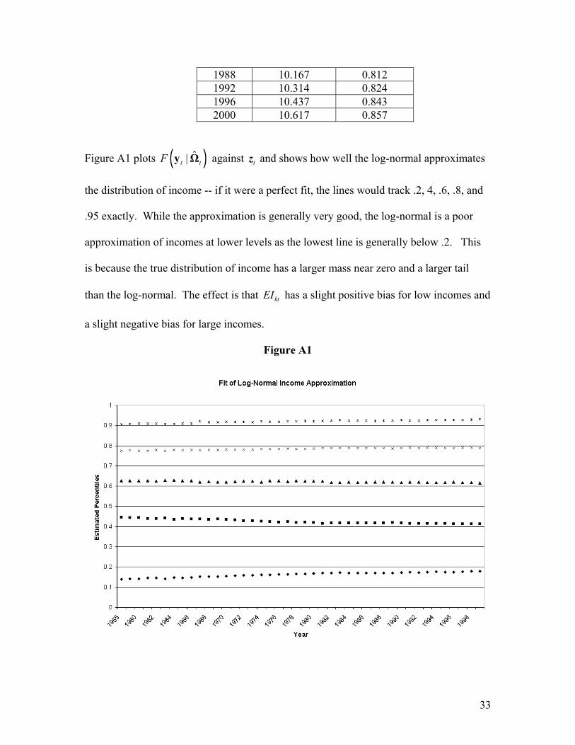
Figure A1 plots ( )ˆ|t tF y Ω against tz and shows how well the log-normal approximates
the distribution of income -- if it were a perfect fit, the lines would track .2, 4, .6, .8, and
.95 exactly. While the approximation is generally very good, the log-normal is a poor
approximation of incomes at lower levels as the lowest line is generally below .2. This
is because the true distribution of income has a larger mass near zero and a larger tail
than the log-normal. The effect is that ktEI has a slight positive bias for low incomes and
a slight negative bias for large incomes.
Figure A1

34
Appendix 2: Measuring Income-Party Stratification
Three complications arise in using the NES to measure the partisanship of the top
and bottom income quintiles:
1. Unrepresentative NES samples: There are several years in which the
distribution of respondent’s income is very unrepresentative of the income
distribution reported by the Census Bureau.
2. NES sample matches neither the “Family” nor “Household” samples for
which the Census Bureau reports income quintiles. The NES asks
respondents for the income of their family for the previous year. For single
voters, the NES asks their individual income. Thus, the NES sample includes
families and single person households. However, the Census family sample does
not include single persons living alone, and the household sample aggregates
multiple families living at the same household, but does include single
householders. Thus, neither Census sample matches the NES.
3. Income quintile measures will often fall within NES income categories. When
a quintile measure falls within an income category, the issue arises as to how to
allocate the respondents in that category into the adjoining quintiles.
It is very difficult to solve all three of these problems for the entire period from
1952 to 2000. Problem 1 necessitates matching the NES sample with the income
distribution from the Current Population Survey, but problem 2 necessitates recomputing
that distribution for units more closely resembling those of the NES. However, even with

35
appropriate measures of the income quintiles, problem 3 has no obvious solution. In
figure 2, we use our log-normal approximation of the distribution of household income to
compute expected income for each NES category. We use these estimates to classify
respondents into income quintiles based on the Census Bureau’s reported income limits
for household income quintiles.
Given the limitations of these choices, we did a number of other calculations to
see if the results in figure 2 are robust. To deal with problem 1, we recomputed the
stratification measures using both household and family income distributions to classify
respondents. We also use samples from the November Current Population Survey’s from
1972 and 1996 which include single individuals and families so as to approximate the
NES population and minimize problem 2.15 Since the November CPS data is categorical,
we use both linear and exponential extrapolation to compute the 20th and 80th percentiles.
Thus, combining all of these data sources, we have four quintiles estimates for 1972 to
1996 and two for each the other years.
To deal with problem 3, we experiment with various ways of allocating
respondents into quintiles. We do four computations for each quintile measure by
including or excluding the relevant NES category in the top and bottom quintiles. Thus,
we have 16 total stratification measure for 1972-1996 and 8 for the other years. Figure
A2 is a “box and whiskers” plot showing the variation across the different measures in
each year. Fortunately, the variation tends to be quite small and the central pattern is
close to that of Figure 2.

36
Figure A2
Box Plot of Stratification Measures
.5
1
1.5
2
2.5 strat
19561960
19641968
19721976
19801984
19881992
19962000

37
References
Acemoglu, Daron and James A. Robinson, forthcoming, “A Theory of Political
Transitions”, American Economic Review. Alesina, Alberto and Roberto Perotti. 1995. “Income Distribution, Political Instability,
and Investment,” European Economic Review 40:1203-1228. Alesina, Alberto and Dani Rodrick. 1993. “Income Distribution and Economic Growth:
A Simple Theory and Some Empirical Evidence,” In Alex Cukierman, Zvi Herscovitz, and Leonardo Leiderman, eds. The Political Economy of Business Cycles and Growth. Cambridge: MIT Press.
Atkinson, A.B. 1997. “Bringing Income Distribution in from the Cold,” The Economic
Journal 107:297-321. Benabou, Roland. 2000. “Unequal Societies: Income Distribution and the Social
Contract,” American Economic Review 90: 96-129. Brady, Henry E. 2001. “Trust the People: Party Coalitions and the 2000 Elections”,
Working paper, University of California, Berkeley. Edlund, Lena and Rohini Pande. 2002. “Why Have Women Become Left-Wing? The
Political Gender Gap and the Decline of Marriage,” Quarterly Journal of Economics 117: 917-962..
Green, Donald, Eric Schickler, and Bradley Palmquist, 2002. Partisan Hearts and
Minds: Political Parties and the Social Identities of Voters. New Haven, Yale University Press.
Kuznets, Simon. 1956. “Economic Growth and Income Inequality,” American Economic
Review, 45:1-28. Londregan, John and Keith Poole. 1990. “Poverty, the Coup Trap, and the Seizure of
Executive Power,” World Politics 62:151-183. McCarty, Nolan, Keith T. Poole, and Howard Rosenthal. 1997. Income Redistribution
and the Realignment of American Politics. Washington D.C: AEI Press. McKelvey, Richard R. and William Zavoina. 1975. “A statistical model for the analysis
of ordinal level dependent variables,” Journal of Mathematical Sociology, 4:103-120.
Meltzer, Allan H. and Scott F. Richard. 1981. “A Rational Theory of the Size of
Government,” Journal of Political Economy 89:914-27.

38
Perotti, Roberto. 1996. “Political Equilibrium, Income Distribution, and Growth,” Review
of Economic Studies. Persson, Torsten and Guido Tabellini. 1994. “Is Inequality Harmful for Growth? Theory
and Evidence,” American Economic Review. Phillips, Kevin. 1990. The Politics of Rich and Poor: Wealth and the American
Electorate in the Reagan Aftermath. New York: Harper Collins. Poole, Keith T. and Howard Rosenthal. 1984. “The Polarization of American Politics,”
Journal of Politics 46:1061-79. Poole, Keith T. and Howard Rosenthal. 1997. Congress: A Political-Economic History of
Roll Call Voting. New York: Oxford University Press. Roberts, Kevin W.S. 1977. “Voting over Income Tax Schedules,” Journal of Public
Economics. 8:329-340. Roemer, John. 1999. “The Democratic Political Economy of Progressive Income
Taxation, Econometrica. 67:1-19. Romer, Thomas. 1975. “Individual Welfare, Majority Voting, and the Properties of a
Linear Income Tax,” Journal of Public Economics. 14:163-185. U.S. Census Bureau; Current Population Survey. Income Limits for Each Fifth and Top 5
Percent of Households (All Races): 1967 to 1999. U.S. Census Bureau (1975). Historical Statistics of the United States from Colonial
Times to 1970. U. S. Census Bureau (2002); “Table F-4. Gini Ratios for Families, by Race and Hispanic
Origin of Householder: 1947 to 2001 (Families as of March of the following year)”; Published 30 September; <http://148.129.75.3/hhes/income/histinc/f04.html>

39
Endnotes
1 The Gini coefficient is the average squared deviation of the income shares of different
percentile groups from proportionality. Other measures of inequality such as the variance
of log income, the proportion of the income going to the top percentiles, and the ratio of
the income of the top quintile to the bottom quintile show essentially the same pattern.
2 This prior trend was so pronounced that it gave Kuznets (1956) the confidence to
argue that increasing equality was a central feature of developed capitalist economies.
3 The literature on the reasons for increased inequality is voluminous, but see Atkinson
(1997) for a good review.
4 The Gini coefficients are taken from U.S. Census (2002). The DW-NOMINATE
scores are based on a scaling of Congresses 1-106. They can be downloaded at
http://voteview.uh.edu/dwnomin.htm. See McCarty, Poole, and Rosenthal (1997) for an
exposition of the derivation of these scores.
5 Computed from Green, Palmquist, and Schickler (2002), Table 2.3, p. 31. The
percentage differences for presidential and midterm election years running from 1972 to
1996 are 25, 30, 32, 36, 34, 35, 36, 34, 36, 29, 38, 48, 50.
6 An important exception (though by a non-academic) is Phillips (1990). This lack of
interest is not true, however, of recent work in comparative political economy that has
sought to link inequality to political conflict and back to economic policy. See Acemoglu
and Robinson (forthcoming), Alesina and Perotti (1995), Alesina and Rodrick (1993),
Benabou (2000), Londregan and Poole (1990), Perotti (1996), and Persson and Tabelini
(1994).

40
7 For example, a major recent work on partisan identification, Green, Schickler and
Palmquist (2002) makes little or no use of the demographic variables employed in this
paper with the exception of a chapter on partisan realignment in the South. They focus
on the stability of individual partisan self-identification. Our focus is on important
changes in how demographics relate to partisan identification. Our main concern is
income but we also find, in addition to the South, an important shift with regard to
gender.
8 Party identification is measured on a seven-point scale in which the categories are
“Strong Democrat, Weak Democrat, Lean Democrat, Independent, Lean Republican,
Weak Republican, Strong Republican”. This is constructed from several questions.
Respondents are first asked to choose between Democrat, Independent, and Republicans.
“Democrats” are then asked if they are Strong or Weak. Ditto for Republicans.
“Independents” are asked if they “lean” to one of the parties. In our analysis of
stratification in Figure 1, we combine the strong and weak Republican categories. In our
ordered probit analysis we use all seven categories. We divide the respondents into
income quintiles using the Census Bureau’s series on the distribution of household
income. The details of the computation of our stratification measure are relegated to the
appendix.
9 Throughout we defined the South as the eleven Confederate states plus Kentucky and
Oklahoma.
10 See Romer (1975), Roberts (1977), Meltzer and Richard (1978), Perotti (1996), and
Roemer (1999).

41
11 As an example, Meltzer and Richard (1978) argue that the optimal linear income tax
rate for voter i is ( ) ( )( ) ( )
1
1 2
1 11 1
ii
i
rt r
r+ η +
=+ η + + η
where the η’s are tax elasticities that are
assumed to be less than 0. Since the elasticities are negative, it is easy to show that t is
decreasing in ri.
12 While this quadratic functional form is difficult to derive from economic
fundamentals, it should be a reasonable approximation.
13 We also estimated the model both with income effects “dummied” for each year and
with each year estimated separately. The separate estimations allow all the coefficients
and thresholds to vary over time. The results were substantively identical. As would be
expected from inspection of figure 2, 1982 and 1998 are least consistent with the general
pattern of the results.
14 For a study that links changes in the income distribution across genders to increased
divorce rates and changes in the partisanship of women see Edlund and Pande (2000).
Since the NES income variable for female respondents records family income for a
respondent from a family and individual income for a respondent from a single-person
household, the fall in female income undoubtedly reflects the increased number of
females now living in single households.
15 We thank Christine Eibner for sharing this data with us.