polygonal simplification techniques class presentation computational geometry comp 290
TRANSCRIPT

Polygonal Simplification Techniques
Class Presentation
Computational Geometry
Comp 290

The Triangle Mesh
• In Computer Graphics, we routinely represent models a polygonal meshes
• Any surface can be approximated by a triangle mesh
• We will assume we have a mesh of triangles that we want to either– simplify, producing one LOD– simplify, producing a succession of LOD’s
Why Simplify the Mesh
• Fewer triangles -- faster rendering speed
• Small detail may not be visible anyway
• Some model acquisition techniques produce models of uniform tesselation. Areas of low curvature don’t need to be as highly tesselated, so simplification may not reduce the quality of the model by much
• Smaller mesh uses less storage space

Pictures of LOD’s

Level Of Detail (LOD)
• Can simplify the same object by varying amounts, producing LOD’s
• Rendering algorithm can intelligently choose LOD in order to obtain:– Obtain constant frame rate, or– Best frame rate that guarantees a certain screen
space error between image rendered with LOD and image rendered with full model

Progressive Mesh• Hugues Hoppe in Siggraph 1996• Defines a continuous sequence of meshes
M0, M1, …, Mn of increasing accuracy• Representation of a model M = Mn:
– a base mesh M0
– n detail records telling how to incrementally refine M0 exactly back to the original mesh Mn
– geomorphs can be efficiently constructed between any two meshes Mi and Mj
• Progressive Transmission

Outline• Triangle Mesh• LOD’s• Progressive Mesh• Competing Goals• Design Parameters• Attributes• Vertex Clustering• Vertex Decimation• Edge Contraction
• Error Bounds• Simplification Envelopes• Pair Contraction• Successive Mapping• Appearance Preserving
Simplification• Multi Resolution
Analysis (wavelets)• Conclusion• References

Competing Goals• Computational Efficiency
• Storage Efficiency
• Quality– Error metrics
• screen space v.s. model space• geometry and attributes
– Global v.s. local optimization• local may be faster• global may simplify more• which gives a better appearance?

Some Design Parameters
• manifold v.s. non-manifold– T-junctions and cracks
• topology preservation– important in some areas– if topology is allowed to change, then we can:
• close holes in objects
• join disconnected components
– when rendering, shape and attribute appearance are more important than topology
Attributes
• Color
• Normal Vectors
• Texture Coordinates
• Curvature
• Material Properties

Outline• Triangle Mesh• LOD’s• Progressive Mesh• Competing Goals• Design Parameters• Attributes• Vertex Clustering• Vertex Decimation• Edge Contraction
• Error Bounds• Simplification Envelopes• Pair Contraction• Successive Mapping• Appearance Preserving
Simplification• Multi Resolution
Analysis (wavelets)• Conclusion• References

Vertex ClusteringRossignac and Borrel, 1993
• Can handle arbitrary polygonal input
• Place a bounding box around original model and divide into a grid
• For each cell, all the vertices in the cell are clustered together into a single vertex
• Update model faces

Vertex ClusteringRossignac and Borrel, 1993
+ Can be very fast
– Often poor quality
– Difficult to construct an approximation with a specific face count
– Grid position and orientation matter
+ Luebke and Erikson, 1997, generalized to use an octree (adaptive grid structure)

Vertex DecimationSchroeder et al., 1992
• Loop until done– For each vertex, measure its distance to the
“average plane” of it’s neighbors– Remove all vertices for which this distance is
below some threshold– triangulate the resulting holes– adjust value of threshold parameter if necessary

Vertex DecimationDecimation Criterion
Distance to plane
Average Plane
Edge Contraction
• Collapse an edge into a vertex
• Used by many simplification algorithms
• Two vertices at the endpoints of the edge get merged into one
• The two faces incident to the edge each contract into an edge
• Only affects local neighborhood

Edge Contraction
Contract
Before After

Outline• Triangle Mesh• LOD’s• Progressive Mesh• Competing Goals• Design Parameters• Attributes• Vertex Clustering• Vertex Decimation• Edge Contraction
• Error Bounds• Simplification Envelopes• Pair Contraction• Successive Mapping• Appearance Preserving
Simplification• Multi Resolution
Analysis (wavelets)• Conclusion• References

Error Bounds
• Given two polygonal meshes P and Q– P and Q are -approximations of each other iff
• every point on P is within of some point of Q, and
• every point on Q is within of some point of P– definition from Cohen et al., 1996
• Given a viewing point and distance, error bounds let us choose the simplest LOD that guarantees a given screen space error

Error Bounds
• Min-# Approximations– given , minimize the number of vertices
• Min- Approximations– given a number of vertices, minimize
• computing minimal-facet -approximation is NP-hard for convex polytopes
• we will look at a few polynomial time approximation algorithms

Simplification EnvelopesCohen, Varshney et al.
• Define a outer and an inner simplification envelope
• Iteratively simplify the model such that the simplified model remains between the two envelopes
• Can preserve sharp edges and boarders
• Can set adaptively across the model

Simplification EnvelopesOffset Surface
• Given a parametric surface– f(s,t) = (f1(s,t), f2(s,t), f3(s,t)), with unit normal
n(s,t) = (n1(s,t), n2(s,t), n3(s,t))
-offset surface is defined as– f (s,t) = (f i(s,t), f i(s,t), f i(s,t)), where
– f (s,t) = fi(s,t) + ni(s,t)

Simplification Envelopes
• A fundamental triangle is a triangle of the original mesh
• It’s fundamental prisim is the volume between the corresponding triangles on the inner and outer envelopes
• The sides of the prisim are bilinear patches
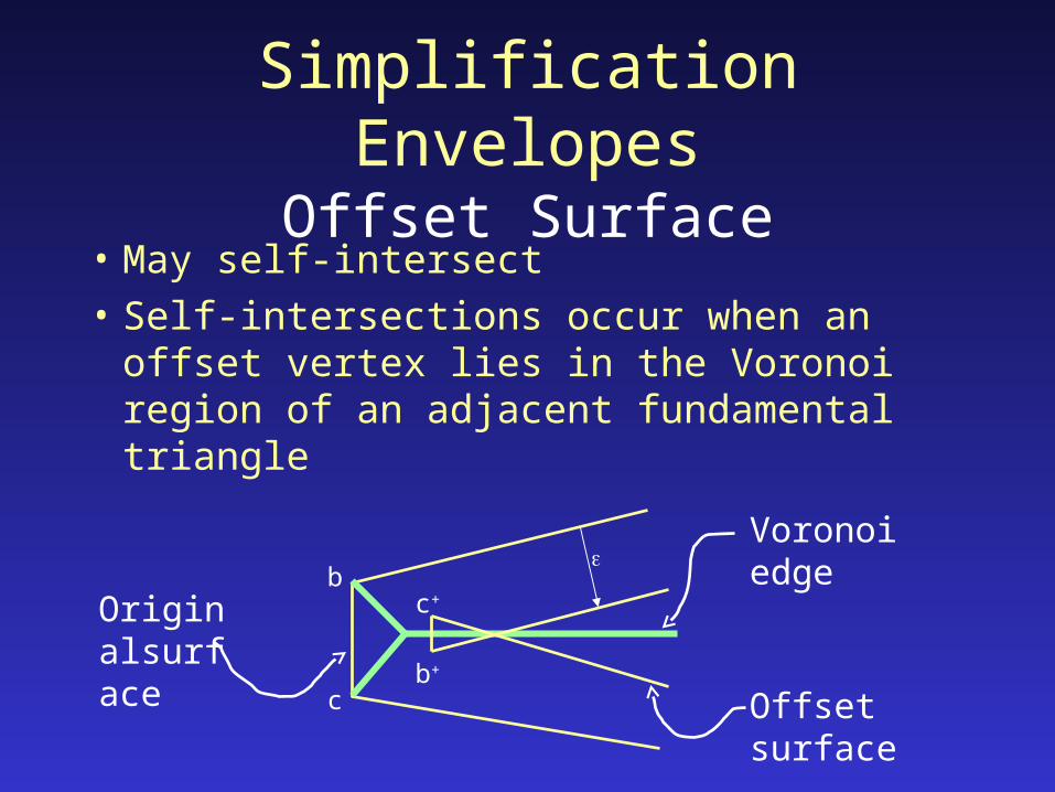
Simplification EnvelopesOffset Surface
• May self-intersect
• Self-intersections occur when an offset vertex lies in the Voronoi region of an adjacent fundamental triangle
Originalsurface
b
cb+
c+
Voronoi edge
Offset surface

Simplification Envelopes
• Simplification envelope is a polygonal surface that lies within from every point p on I in the same (or opposite) direction as the normal at p
• Outer envelope is in the direction of the normal, inner envelope in opposite direction
• Reduce where necessary to avoid self-intersections

Simplification Envelopes
• Start with input surface
• Iteratively modify– hole creation: remove a connected set of
triangles from the mesh– hole filling: fill the hole with a smaller number
of triangles
• Holes must be filled with triangles that lie between the two envelopes

Decimation via Pair ContractionGarland and Heckbert, 1997
• Edge contraction generalized to pair contraction between arbitrary vertices– (v1,v2) v’
– merges v1 and v2 into one vertex v’– connects incident edges– remove edges or faces that have become
degenerate
• Local control--only affects neighborhood

Decimation via Pair Contraction
• Pair Contraction can alter topology– fill holes– connect previously disconnected components
• Handles non-manifold surfaces
• Error is approximated with quadrics– Not sure what this means geometrically; I can’t
gain intuition from the math– Used to maintain a cost function
• characterization of error at each vertex

Decimation via Pair ContractionAlgorithm
• Select all valid pairs• Initialize cost function
• Select valid pairs (v1,v2) of vertices st.
– (v1,v2) is an edge, or
– |v1,v2| < t, where t is a threshold parameter
• Compute cost of contracting each valid pair• Place pairs in a heap sorted by cost• ...

Decimation via Pair ContractionAlgorithm continued
• ...
• Iteratively– remove from heap pair (v1,v2) of least cost
– contract (v1,v2)
– update cost of all pairs involving the vertices
• Produces a progressive mesh

Outline• Triangle Mesh• LOD’s• Progressive Mesh• Competing Goals• Design Parameters• Attributes• Vertex Clustering• Vertex Decimation• Edge Contraction
• Error Bounds• Simplification Envelopes• Pair Contraction• Successive Mapping• Appearance Preserving
Simplification• Multi Resolution
Analysis (wavelets)• Conclusion• References

Successive MappingCohen et al., 1997
• This algorithm is really cool!– Uses lots of ideas from computational geometry– Gives tight error bounds on geometry– Defines a piece-wise linear mapping between
original surface and simplified surface– Can produce a progressive mesh– Algorithm tracks error both from original
surface and from previous level of detail

Successive MappingHigh-level Algorithm
• Generic greedy algorithm
• Measure cost of all possible edge collapses
• Loop until no edged can be collapsed– collapse edge with least cost– (locally) re-compute cost of affected edges
• Output– original model– ordered list of edge collapses and assoc. cost

Successive MappingNaïve Approach
• Use natural mapping (picture from Cohen et al.,1997)
• Does not map from simplified surface back onto original surface
• Error may be larger than necessary

Successive Mappingplanar projection
• Cohen performs mapping using a planar projection of the local neighborhood called successive mappings
• Find a valid direction of projection that is one-to-one
• Re-triangulate in this plane
• Guaranteed no self-intersections if mapping is one-to-one
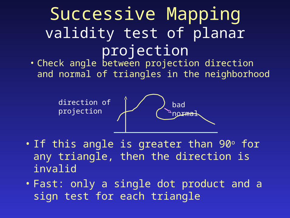
Successive Mappingvalidity test of planar projection
• If this angle is greater than 90o for any triangle, then the direction is invalid
• Fast: only a single dot product and a sign test for each triangle
direction of projection bad normal
• Check angle between projection direction and normal of triangles in the neighborhood

Successive Mappingfinding valid projection
• Gaussian sphere unit sphere where each point corresponds to a unit
normal vector with same coordinates
• For each triangle, define a plane through the origin with the same normal as the triangle
• A projection direction if valid w.r.t. a triangle iff it its point on the Gaussian sphere lies on the correct side of this plane
• There is a half-space of valid directions
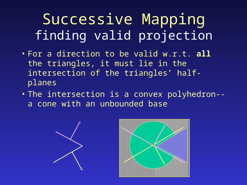
Successive Mappingfinding valid projection
• For a direction to be valid w.r.t. all the triangles, it must lie in the intersection of the triangles’ half-planes
• The intersection is a convex polyhedron--a cone with an unbounded base

Successive Mappingfinding valid projection
• Bound the last face by adding 6 more half-spaces--the faces of a cube containing the origin
• Construct a valid projection direction by finding a point inside the intersection and normalizing it’s length
• Use linear programming
Successive Mappingplacing new vertex
• Topology of mesh after edge collapse is determined, but we get to choose where to place the edge
• Orthographically project into a plane in the projection direction the neighborhood of the edge to be collapsed
• A valid position for the vertex is one that causes no edge crossings
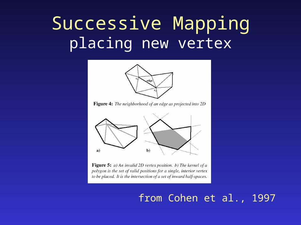
Successive Mappingplacing new vertex
from Cohen et al., 1997
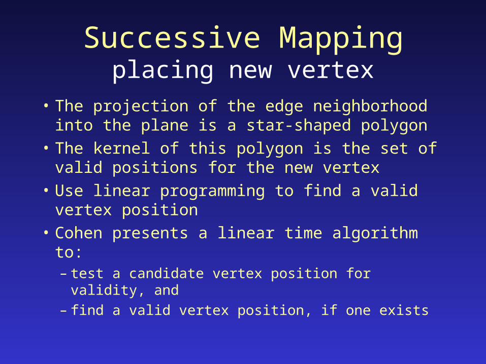
Successive Mappingplacing new vertex
• The projection of the edge neighborhood into the plane is a star-shaped polygon
• The kernel of this polygon is the set of valid positions for the new vertex
• Use linear programming to find a valid vertex position
• Cohen presents a linear time algorithm to:– test a candidate vertex position for validity, and– find a valid vertex position, if one exists
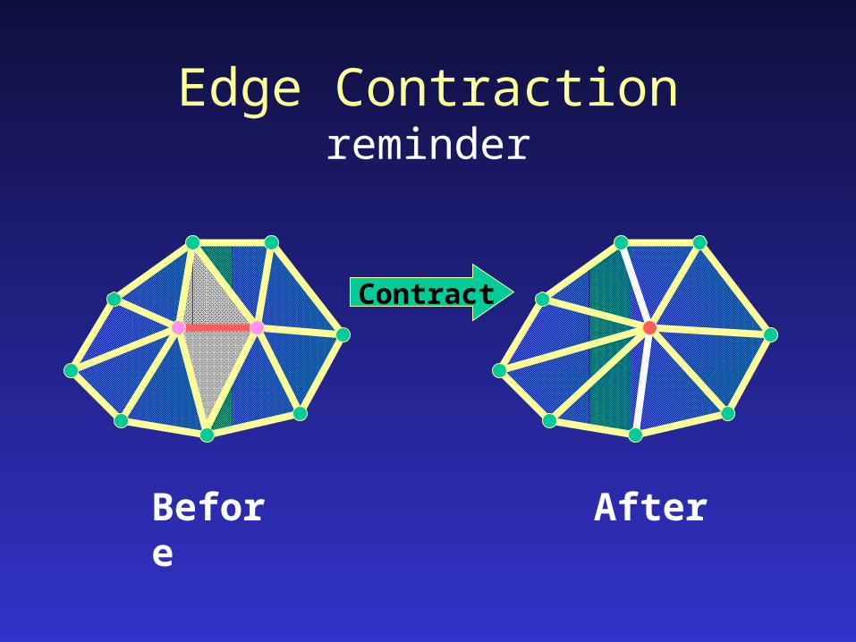
Edge Contractionreminder
Contract
Before After
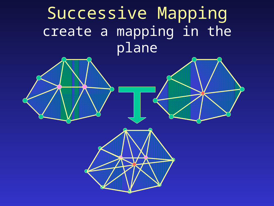
Successive Mappingcreate a mapping in the plane
Successive Mappingfind 3D vertex position
• We now have a piecewise linear mapping from the two local neighborhoods
• This mapping will serve as a mapping between the two successive meshes if we project each point back to the surface in the direction of projection
• The 3D position of the new vertex must lie on the line parallel to the direction of projection and passing through the its 2D position in the plane
• Finding its position is all we have left to do

Successive Mappingoptimize 3D vertex position
• Because the triangles are planar, the maximum distance between any two must be at the boundary– For these triangles, it must actually be at a vertex
– The distance between respective border vertex positions is zero--they didn’t move
• Parameterize the position of the new vertex along the line by the single parameter t– as t varies, the distance from an interior vertex to it’s
mapped position on the other surface varies linearly
– optimize t to minimize the maximum distance

Successive Mappingbounding the error to original surface
• Maintain a region that bounds the error between each LOD and the original surface
• Incrementally update the bounding regions in the local neighborhood of each edge collapse operation– The portion of the original surface
corresponding to a given triangle lies within the convolution of the triangle and the bounding volume

Appearance-Preserving SimplificationCohen et al., 1998
• This algorithm is even more cool!– Improves on Successive Mapping algorithm– Projects into texture space instead of arbitrary
plane– Handles texture coordinates, normals, and other
attributes gracefully, providing error bounds– Decoupled representation

Appearance-Preserving Simplification
• Can create not only texture maps, but also– maps for other scalar fields– maps for vector fields, e.g., like normal maps
• This algorithm– decouples the normal field from the geometry– defines a texture deviation metric to guarantee
bounds on texture coordinate deviation– total error metric - combines both geometric and
texture error metrics

Appearance-Preserving Simplification
• Algorithm similar to Successive Mapping, but instead of projecting into a plane, project into texture space
• Extra bookkeeping to track texture error
• Normal mapping lets the simplified model use the normals from the original triangles
Multiresolution Analysis• Elegant theoretical approach using wavelets• Quite a few papers using this approach• Store a base mesh along with the wavelet
coefficients• Applications include:
– compression as well as simplification– progressive display and transmission– LOD control– multiresolution editing

Outline• Triangle Mesh• LOD’s• Progressive Mesh• Competing Goals• Design Parameters• Attributes• Vertex Clustering• Vertex Decimation• Edge Contraction
• Error Bounds• Simplification Envelopes• Pair Contraction• Successive Mapping• Appearance Preserving
Simplification• Multi Resolution
Analysis (wavelets)• Conclusion• References

Conclusion
• Many types of simplification algorithms– guarantee different things– running times vary
• What’s the right one for me?– depends on the application

References
Cohen, Varshney, Manocha, Turk, Weber, Agarwal, Brooks, and Wright, Simplification Envelopes, Siggraph’96
Cohen, Manocha and Olano, Appearance-Preserving Simplification, Siggraph’98
Garland and Heckbert, Surface Simplification Using Quadric Error Metrics, Siggraph’97
Hoppe, Progressive Meshes, Siggraph96
Schroeder, Zarge and Lorensen, Decimation of Triangle Meshes, Computer Graphic July 1992
Turk, Re-Tiling Polygonal Surfaces, Computer Graphics July 1992
• For a starting point to find papers on Multiresolution Analysis– Eck et al., Multiresolution Analysis of Arbitrary Meshes, Siggraph’95