polymer blends and alloys course outcomes · polymer blend (or binary system). • binary=2,...

Polymer Blends and Alloys

[Note: contents of these notes are compiled from various sources to cover the course syllabus, made for self study

purpose. It is for fast reference, & hence for detailed information, the textbooks shall be referred. Suggestions are

welcome. Apart from this typed notes, even the class discussions which are noted by students are equally important,

some of which are not covered in this due to shortage of time. While answering, please understand & write to the

point without much of extra information which is given in notes below. Answer question number wise & use

statistical approach to be precise.]

Course outcomes: Upon successful completion of this course, the student will be able to

understand-

CO1- the fundamentals of polymers blends and blending equipments;

CO2- thermodynamic aspects, phase diagram and morphology of blends;

CO3- miscibility and characterization of blends;

CO4- the mechanism and approaches of compatibilization and toughening;

CO5- interpenetrating polymeric networks, and Design polymer blends/alloys system to meet the

requirements.

[Percentage of POs & CLs covered & mapping with COs.]

Course material: Unit-1 (foundation Unit, important one- because the basics covered in this unit will be

utilized directly in other units, So, while answering any question of other 4 units, students shall mention information

from this unit accordingly)

Definitions:

• Polymer Blend: Mixture of two or more polymers. (The second polymer added will be of

significant quantity i.e. > 2% by weight).

• Polymer Alloy: compatibilized polymer blend.

Some distinctions for clarity:

• Copolymer (Cop): Polymer formed by two or more types of- repeating units or co-

monomers.

• Polymer Compound: Mixture of polymer and additives/ingredients (from any material

class).

• Polymer Composite: Any combination of polymer and filler in any form (from any

material class).

• Solid state Material classification: Polymers, Metal, Ceramics.

• Polymer Crosslinking/ curing/ vulcanization: process of getting 3 dimensional networks

of polymeric chains. (by chemical bonds)

• Physical cross links results out of localized crystallization/ interactions due to secondary

forces / entanglements.

• Interpenetrating Polymeric Networks (IPNs) can be of both types (i.e. resulting from

physical/chemical crosslinks).

• Thermoplastic Elastomers (TPEs) - polymeric materials behaving like rubbers & having

processibility of thermoplastics. [could be achieved via blends/ cop/ chemical or physical

cross linking]

• Polyelectrolytes/ ionomers/ ionic polymers: polymer backbone with 1 kind of charge

(an/cation) & pendant/side groups with another kind of charge.

• Miscible - Homogeneous mixture in any proportion [will be homogeneous at molecular

level].

• Soluble- Homogeneous mixture in limited proportion (up to saturation level).

• Homogeneous- just means same, & can be wrt morphology/ orientation/ distribution.

• Compatible: to work harmoniously (so they can be heterogeneous or immiscible but yet

perform harmoniously without losing original properties).

• State: usually 3 states of matter- solid, liquid & gas (just based on molecular packing at

physical level).

• Phase: sometimes used as synonymous to state but here the phase difference arises due to

chemical and/or physical differences, any material or combination of materials exhibit

distinct phases. For example in the liquid state mixture of water & oil, we can observe

two phases. Semi-crystalline polymers show phases of crystalline region & amorphous

region. Immiscible polymers shows phase separation.

• Compatibilization: Incompatible/ Immiscible blend + compatibilizer � to get � Alloy

(this can still possess phases).

• Interphase: a third phase [of about 2-60nm] between the two phases of immiscible

polymer blend (or binary system).

• Binary=2, ternary=3.

• Toughened polymer: brittle polymer with increased toughness [mixing with rubber (for

low temp. application)/ with engineering plastics (for high temp. application)/ with little

plasticizer/process aid/ toughener (is a compounding approach)].

• Morphology: study of micro structure. Microscope assists the study of various phases.

• Physical compatibilization: achieved by changing temperature, pressure, rate of mixing,

radiation, δ H, δS , co- dissolution. [δ G = δ H − TδS]

• Specialty polymers – stable up to 5000C.

• Aromatic/ Engineering polymer’s properties can be 500 times more than that of aliphatic/ Commodity

Polymers [e.g. mechanical property of aliphatic polyester is 70 Mpa & that of aromatic polyester 4000 Mpa.]

• E.g. of blends: PC/ABS (mobile panel), PS/BR (HIPS), PS/ PPO, PMMA/SAN, NR/GP

(gutta purcha), PE/PP. Blends are represented using “/” symbol between the polymers

and it should not be read as “or” as we do in other case! The second polymer is referred

to as second component, & denoted as: X2 or Xb or φ2 or φb.

Need for blending (the driving force): instead of carrying out research in developing new

monomers/ polymers/ copolymers with required set of properties as per requirement, and to

establish it across the market, which consumes lot of time, money & energy; it is worth

developing a blend with existing materials with known properties.

Classification of polymer blends: on various basis-

• Based on polymer type:

o Thermoplastic/thermoplastic

o Thermoplastic/rubber

o Rubber/rubber

o Rubber/thermoset

o Engineering plastic/rubber, etc

• Based on component interaction:

o Miscible/ immiscible

o Compatible/ incompatible

• Based on application (i.e. performance at high temperature & high load) :

o Commodity blend

o Engineering blend

• Homologous polymer blends: Blend of polymers in order of molecular weight.

• 3 Types of mixtures based on performance (i.e. components interaction leading to

property changes):

Mixture type Effect

Additive A+B = (A+B)

Synergistic A+B > (A+B)

Antagonistic A+B < (A+B)

Blends can also be classified as above.

Important Characteristic of blend is “Phase behavior”. That is, the 2 or more polymers when

mixed may show following phase behavior:

Whether a blend should be miscible or not depends on application requirements, for example,

HIPS is immiscible blend of PS & BR where 2 phases are separated as shown below, & is used

in market for some applications:

And, if compatibility is required then it is compatibilized addingg SB block copolymer as

compatibiliser. It helps distribution of load, and also propagation of load takes place gradually.

Therefore better tensile properties are achieved than unmodified HIPS as required for some

applications.

Advantages/ Reasons for blending:

� To extend engineering resin performance by diluting it with low cost (commodity/

tonnage) polymer.

� To develop materials with a full set of desired properties.

� To utilize the scrap generated at various steps. [sometimes blending is also done

to develop a recyclable material, e.g. using starch as second component]

� To get a high performance blend from synergistically interacting polymers.

� To achieve customer specifications in a product.

� Reduced R&D expenses & the time consumed in developing new monomers &

polymers to yield a similar property profile.

� Lower capital expense involved with scale-up &commercialization.

How to Design a Polymer Blend? Steps:

1. Define the physical and chemical properties the ideal blend should have.

2. From a list of resin properties, select those polymers which may provide some of the

required behavior (usually a wider range of desired properties requires several types of

potential candidates).

3. Tabulate the advantages and disadvantages of the selected resins. There must be

alternating candidates capable of providing each of the required properties.

4. From the list of candidates, select a set of resins which assures most suitable

complementarily properties.

5. Determine the miscibility of selected resins and method of making them compatible if

needed.

6. Examine the economics, compatibilization, compounding, as well as the effect of

forming, maintenance, longevity, etc.

7. Define the ideal morphology which will assure the optimum performance of the finished

product.

8. Select the rheological properties of the blend components, concentration of ingredients,

amount of compatibiliser, type and intensity of deformation field needed for generating

the pre-cursor morphology.

9. Determine the method of stabilizing the morphology e.g. by controlled cooling rate,

crystallization, chemical reaction, irradiation, etc.

10. Select the optimum fabrication method which will assure formation of the final

morphology (if not achieved go back to step 8.)

Limitations of blending:

• Recycling is complex in some cases.

• No specific test methods and standards are available. (used that of plastic/rubber)

Criteria for selecting the blend components:

� Principle advantages of 1st polymer (base polymer or component one) should compensate

for deficiencies of the 2nd polymer; and vice versa.

E.g.: Disadvantage of PPE (processibility & impact strength are compensated by

advantageous properties of HIPS.

� Complex balance of property is usually achieved by multi-component blending with

some unavoidable compromises {such blends can play multiple roles- mechanical

properties, chemical resistance, dimensional stability, paint ability, etc., e.g.:

PC/TPE/Latex System.}

Methods of blending: Solutions mixing/ melt mixing/ mixing above Tg/ mix one polymer in

another monomer & polymerize/ mix two monomers & polymerize simultaneously/ latex

mixing/ powder mixing & processing.

• Mechanical mixing: mechanical mixing of polymers includes such methods as roll

milling and melt mixing.

o In roll milling, the mixing of polymers can be accomplished by squeezing the

stock between the rolls.

o In melt mixing the polymers are mixed in the molten state. E.g. in extruder.

• Dissolution in co-solvent (followed by film casting, freeze/spray drying)

• Latex blending: Emulsion polymerization is employed for the preparation of rubber

toughened plastic blends. The polymers should be in the latex or emulsion form. The

mixing process of these micro-sized latexes and the subsequent removal of water produce

excellent dispersion.

• Fine powder mixing: In this method components are taken in powder form and mixed.

Followed by suitable processing technique.

• Use of monomers as solvents for another blend component, followed by polymerization

as in interpenetrating networks.

Mixers for blending polymers: Mixers can be used either batch or continuous types.

Under batch mixers there are of three types namely:

• Roll mills (exposed)

• Sigma blade mixer (internal mixers)

• Kinetic energy mixers.

� Sigma blade mixers: Sigma Blade batch systems provide complete, homogeneous

mixing, even in small quantities. The vessel and moving parts inside are designed to

ensure consistent granulation action, and a predictable homogeneous blend in a broad

range of products. A special breaker ensures movement of elements to eliminate dead

spots and ensure all material are blended thoroughly and granulated consistently.

Sigma blade Mixer Operation: the tangential action of mixing and kneading is thoroughly

obtained by 'Z' (SIGMA) shaped kneading blades, which rotates very accurately at different

speed towards each other causing product to be transferred from blade to blade. Discharge of the

mixed product is achieved by tilting the container or through the valves at the bottom or by

means of an extrusion screw below the container if provided.

Continuous mixers:

� Single or twin screw extruder.

� Dynamic melt mixer.

� Disc extruder.

� Twin shaft intensive mixer/single-shaft.

� Motionless mixer also called static mixer.

� Repro CTM mixer.

Special machines:

• Plastificator patfoort.

• Reverser.

• Multistage systems.

Reactive extrusion: process where the reactive site incorporation and melt extrusion of blends is

carried in a single pass extrusion operation. The reactive extrusion compatabilization has been

one of the most practical methods employed for achieving mechanical compatibility for many

diverse polymer blends. Commercial example includes EPR toughened PA called as “super-

tough nylon”, Polyolefin/PVAOH [an extreme example of incompatibility because of hydrophobic

& hydrophilic (hygroscopic) or non-polar & polar natures polymers respectively].

Fig. Reactive extrusion of PO/PVAOH blends using twin screw extruder with 12sections

The design & operation of extruders as reactors for conducting single pass operation

allowing for economic advantage has been noted in several book chapters.

Examples of some commercial blends & its applications:

• < Elastomer blends- Tyre application >

• <Emulsion blends – Adhesion & coating application >

• PVC/Nitrile rubber � To overcome migration of plasticizers in PPVC

• There are various parameters which contribute to miscibility or immiscibility of any blend.

Viz. type of polymers, composition, molecular weight, crystallinity, polarity, temperature, H-

bonding/ secondary forces of interactions, mode of blending, solubility parameter difference,

Gibbs free energy, etc. [it needs deep study to know ‘what influences how much’ in each case

of blend system using knowledge & analytical techniques].

• Here is an example which sounds irrational: PMMA is incompatible with PS, & PMMA

is also incompatible PAN, but PMMA is compatible with SAN, which is a copolymer of

repeating units of previous 2 polymers with which it was incompatible!

• Para (hexa fluro 2-hydroxy isopropyl) styrene & polystyrene co-polymer is compatible

with PC, PMMA, PVAc, etc. this is an example to show how functionalization of a

polymer can bring in compatibility with many polymers.

• HDPE & PP forms immiscible blends, though polarity, solubility parameter & secondary

interactions matches; here, the crystallinity difference overtakes leading to immiscibility

of these two polyolefins. [by nature, any system tends to be more random, but in above

case, as blending forces them to be more crystalline, they oppose to be miscible and

continue in their randomness]

• PPO/PS is a miscible blend due to overlapping of aromatic rings of both polymers. This

is developed for easier processing of PPO. Because, PPO’s Tg is 2100C & processing

temperature would be still high plus melt viscosity is also high, where as PS’s Tg is1000C

& helps easy processing of PPO.

• Blends of crystalline thermoplastics and amorphous rubbers are developed to achieve a

combination of low temperature flexibility &high temperature resistance; e.g. the TPOs

[thermoplastic polyolefines class of TPE] used for automobile part applications.

Unit-2

Morphology:

• Even the phase morphology do change depending on various parameters as mentioned

above plus the processing, post treatments, way of cooling, etc for e.g. In HIPS, phase

inversion is observed if BR composition is increased, then BR becomes a co-continuous

phase, & still further becomes a major continuous phase and then PS becomes

discontinuous or minor phase, if same is extruded then the spherical morphology

becomes rod like cylindrical [recall all those morphology structures studied in

analysis subject & use them over here]; which increases tensile properties of HIPS, as

it acts like Composites. [I.e. fiber like structure inside the matrix]. In case of

PBT/PVAOH� Lamellae (sheet) morphology is achieved when it is biaxially oriented

<using stretch blow molding /blow film extrusion or via cross head extrusion>, this is

used in container application like bottles to have 2 layers of polymers with different

properties as required for application like- the one used to contain carbonated beverages

because, carbondioxide cannot pass through Poly Vinyl Alchol, so, soda remains fizz.

[note: in Mackintosh (rain coat) outer layer is of rubber to protect from water & inner

from (cellulose) cotton to feel comfort by absorbing sweat, this arrangement is not blend,

this is an example of composite.]

Miscibility depends on temperature and composition also:

Phase diagram (to show temperature dependency on miscibility)

In the above figure of temperature versus composition [phase diagram for blends

or solutions or any mixtures], the shaded region represents phase separation & outer

boundary the single phase (miscible region). It says that, depending on type of material,

the temperature at which a mixture is miscible varies with composition.

LCST: Lower critical solution temperature- the lowest temperature below which all

compositions are miscible.

UCST: Upper critical solution temperature- the highest temperature above which all

compositions are miscible.

Schematic of free energy vs composition for systems of limited solubility: Phase diagram (to

show composition dependency on miscibility)

At any composition less than B1 and greater than B2 a single phase (given by the solid curve) as

lower free energy then any 2 phase system with the same overall composition. i.e. at these

compositions only one phase will exist. For compositions in between, the system will consist of

two phases of composition B1 and B2.Figure shows miscibility variation of blend A/B, where

B’s composition at 30 & 70 % are favorable in getting a more miscible blend (because low Gibbs

free energy) than that between 30 and 70% composition. [Note: the y-axis is delta Gmix].

Note: In a blend which is immiscible, additives reside usually in the softer region (softer

polymer).

Phase diagrams of composition vs Temperatures (ф-T) observed with various polymer

blends

• The phase diagrams of polymer mixtures can take many forms as shown in figure below

where the single phase and phase separated regions exists in the composition temperature

range depicted. Many miscible systems i.e. (a), exhibit miscibility over the entire

composition temperature range where both polymer exhibit thermal stability. Miscible

system where the level of miscibility is border line will often show phase separation

within the experimentally determined ф-T space LCST and UCST i.e (c) and (d), have

been observed in many polymer blends; and both were observed in rare cases i.e (e). The

hour glass diagram depicts overlapping LCST and UCST behavior i.e (f), (e.g. a study

involving PS and poly pentyl methacrylate showed this behavior). The most common

case is as in (b), where the phase separated regions comprises the majority of the T-ф

phase.

With all immiscible blends, each phase will contain both polymers. However, with highly

immiscible blends, the concentration of the second polymer in a polymer rich phase will

be extremely low and have an undetectable influence on the properties of that phase.

Double LCST and double UCST i.e (g) and (h), behavior can be obtained via the

equation of state theory predictions. All of the diagrams shown in figure below have been

experimentally observed and also can be predicted from various theories. [usually got by

varying components, composition, T, P, MW, etc]

Phase diagrams observed with polymer blends <shaded area= phase separated region>

Resultant property after mixing two polymers:

[Case: miscible blend]

The property value of blend will be in between that of the two polymers’

property values, depending on composition. But, depending on interaction, this trend may

slightly vary too! Consider the example of Tg variation of blends as shown in typical plot.

Polymer A has low Tg, & polymer B has high Tg, so, with increase in composition B, this

miscible blend surely shows increase in Tg, but if blend components have i) strong interaction-

then the property increase will have higher profile; & if blend components have ii) weaker

interaction- the property increase will have lower profile .

Property variance in miscible blend & its dependency on interaction

[Case: all types]

If the straight line joining the 100% composition point of A at left to the 100%

composition point of B at right is considered as median, then the curves above and below this

shows the way in which property varies

blends the properties will increase than that of 2 components & for antagonistic blends the

properties will be lower than that of two, and for others it will be varying in between

depending on miscibility, interaction & composition (at a given te

Approaches for achieving miscib

Hydrogen-bonding

Dipole –dipole interaction




shows the way in which property varies for differently interacting blends. For sy



depending on miscibility, interaction & composition (at a given temperature).

Approaches for achieving miscibility & compatibility:




for differently interacting blends. For synergistic



mperature).

Matched solubility parameter Parameters for Miscibility

Ion –dipole interaction

Mean field approach

Association model

Ternary non-reactive component addition

Block &graft co polymer addition

Reactive compatibilization Approaches to get alloy

(Compatibility of phase separated blends)

Co-crosslinking

Interpenetrating networks

In-situ polymerization

Nano particle addition/ additives

Thermodynamic relationships for polymer blends

Thermodynamic conditions for miscibility are:

Note: both the conditions should be satisfied for miscibility, else phase separation will

predominate.

Two mechanisms of phase separation:

i. Nucleation and growth

ii. Spinodal decomposition

For nucleation, the new phase must initiate with a composition which is not near to that of parent

phase. Nucleation is a phase transition, which is large in degree i.e. composition change but

small in extent i.e. size; whereas spinodal decomposition is small in degree but large in extent.

Comparison between Spinodal Decomposition and Nucleation and Growth

• An initially homogeneous solution develops fluctuations of chemical composition when super

cooled into the spinodal region. These fluctuations are at first small in amplitude but grow

with time until there are identifiable precipitates of equilibrium composition.

• In contrast, during nucleation and growth, there is a sharp interface between the parent and

product crystals; furthermore, the precipitate at all stages of its existence has the required

equilibrium composition.

Spinodal decomposition involves uphill diffusion, whereas diffusion is always down a

concentration gradient for nucleation and growth of the type illustrated below. Spinodal

decomposition refers to a mechanism of phase transformation inside a miscibility gap. It is

characterized by the occurrence of diffusion up against a concentration gradient, often referred as

“uphill” diffusion, leading to formation of a uniform-sized, periodic fine microstructure.

Figure: Direction of diffusion depicted by arrows in spinodal decomposition (top) and nucleation

and growth (bottom).

Figure shows interconnected bicontinuous morphology of A rich and B rich phases. Nucleation

and growth results in the formation of spherical particles dispersed in a matrix. Those particles,

having a size greater than the critical nucleus would grow with time, at the expense of the

smaller particles due to Ostwald ripening (info).

Table: Comparison of Phase Separation Processes.

Property Nucleation and Growth Spinodal Decomposition

Size of phase separated region increases with time size constant

Concentration of phase separated region constant with time increases with time

Diffusion coefficient positive negative

Phase structure separated interconnected

Activation energy required not required

Region of phase diagram metastable or unstable region only unstable region

Fig. a) Nucleation and Growth with spherical particles dispersed in a matrix, b) Spinodal

decomposition with an interconnected bicontinuous morphology.

Reasons why classical diffusion equation fails to describe the spinodal decomposition process

can also be understood by looking at free energy reduction.

the free energy reduction. In the case of mass flow, this driving force manifests itself as

equalizing chemical potential. [i.e. As Energy flows till temperature becomes equal, and as

volume changes till pressure becomes equal, so is this mass flow till ch

equal] . Even though in classical cases such free energy reduction is also accompanied by decay

of decompositional heterogeneities, in the case of spinodal it is not so. In the case of SD, ‘the

homogenization of chemical potentials

Fick’s law is modified for this case.

[Note: recall the sketch drawn in class with two frames, which is important]

• The spinodal cure is related to position where

• A spinode is a cusp where 2 curves meet

stability of a solution to decomposition into multiple

• Binodal or co- existence curve or bin

system i.e. it is a boundary between mixed &




ooking at free energy reduction. The driving force for any process is



volume changes till pressure becomes equal, so is this mass flow till chemical potentials become

in classical cases such free energy reduction is also accompanied by decay


homogenization of chemical potentials leads to the heterogeneities in composition’, therefore

Fick’s law is modified for this case.


The spinodal cure is related to position where

A spinode is a cusp where 2 curves meet or a stationary point of curve

stability of a solution to decomposition into multiple phases is referred to as spinodal.

existence curve or binodal curve is the condition of miscibility f

t is a boundary between mixed & separated phase therefore it is a condition at




The driving force for any process is



emical potentials become

in classical cases such free energy reduction is also accompanied by decay


leads to the heterogeneities in composition’, therefore


or a stationary point of curve. The limit of

is referred to as spinodal.

odal curve is the condition of miscibility for a binary

separated phase therefore it is a condition at

which 2 distinct phases

drawing a tangent line to free energy.

• The critical point where the bino

expression

• The knowledge of extent of P

rather to rather device for methods for blend modification to

modulus, HDT IS, etc.

• The miscibility provides a

compatibilization method.

• In a system store phase separation occurs within

temperature (T), Pressure (P), Concentration of

particular attention to miscibility may lead to highly successful product.

• Miscibility defines flow behavior & orientation effect i.e. performance of finished

product.

• Self-diffusion co-efficient of macro

thermodynamic conditions are difficult to achieve.

• Even though near equilibrium conditions are obtained in processing equipment

&extrusion] they are not necessarily preserved in the finished product.

• P-P miscibility is determined by a

significantly smaller than those observed in small molecules solution.

• Whenever a process goes from one s

in properties like H, G, S, X

Thermodynamic relationship for mixtures

The most important relationship governing mixtures of dissimilar components say

which 2 distinct phases may co–exist & can determined at a given temperature by

drawing a tangent line to free energy.

The critical point where the binodal & spinodal intersect is determined from the

The knowledge of extent of P-P miscibility is not only important to produce miscible but

rather to rather device for methods for blend modification to enhance properties

The miscibility provides a simpler means of accomplishing this than other types of

compatibilization method.

In a system store phase separation occurs within accessible range of variables [i.e.

temperature (T), Pressure (P), Concentration of components], the processes

particular attention to miscibility may lead to highly successful product.

Miscibility defines flow behavior & orientation effect i.e. performance of finished

efficient of macro molecules is of low value, t

thermodynamic conditions are difficult to achieve.

Even though near equilibrium conditions are obtained in processing equipment

they are not necessarily preserved in the finished product.

P miscibility is determined by a delicate balance of enthalpic &

significantly smaller than those observed in small molecules solution.

Whenever a process goes from one state to another state say for e.g. mixing,

S, Xb, µ, etc do change and are given by:

∆G = G − G0

∆H= H − H0

∆S = S − S0

Thermodynamic relationship for mixtures (i.e. for miscibility of polymer blends)

The most important relationship governing mixtures of dissimilar components say

∆Gm= ∆Hm- T.∆Sm ------------ (3)

exist & can determined at a given temperature by

spinodal intersect is determined from the

only important to produce miscible but

enhance properties like

of accomplishing this than other types of

accessible range of variables [i.e.

, the processes with a

Miscibility defines flow behavior & orientation effect i.e. performance of finished

thus equilibrium

Even though near equilibrium conditions are obtained in processing equipment [I/M

entropic forces,

mixing, the change

(i.e. for miscibility of polymer blends):

The most important relationship governing mixtures of dissimilar components say ‘A & B’ is-

Where, ∆Gm = free energy of mixing

∆Hm = enthalpy/heat of mixing

∆Sm = entropy of mixing

T = temperature (any fixed or considered temperature)

I. Entropy of mixing:

To understand the extent of combinatorial entropy contributions for miscibility of polymer

blends, let us consider interactions between following 3 cases:

A. Solvent - Solvent

B. Polymer – Solvent

C. Polymer – Polymer

In low molecular weight components i.e. case-A, combinatorial entropy is major

contribution for miscibility Therefore, solvents show broad range of miscibility; whereas it is

less between polymer & solvent i.e. case-B; and still less for polymer & polymer, i.e. case-C. So,

contribution of combinatorial entropy is very less for miscibility of polymer blends.

For low molecular weight materials, generally increase in temperature leads to

miscibility, as T∆S increases and ∆G decreases; but, for higher MW components i.e. for

polymers T∆S is small and other factors like non–combinational entropy combinations and

temperature dependent ∆H values can dominate and lead to the reverse behavior namely,

decrease in miscibility with increase in temperature. Thus, for case-A & case-B, UCST exists

and for case-C, LCST exists!

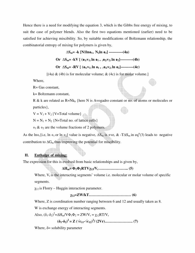
Hence there is a need for modifying the equation 3, which is the Gibbs free energy of mixing, to

suit the case of polymer blends. Also the first two equations mentioned (earlier) need to be

satisfied for achieving miscibility. So, by suitable modifications of Boltzmann relationship, the

combinatorial entropy of mixing for polymers is given by,

∆Sm= -k [N1lnɸɸɸɸ1+ N2ln ɸɸɸɸ2] -----------(4a)

Or ∆Sm= -kV [ (ɸɸɸɸ1/v1) ln ɸɸɸɸ1 + (ɸɸɸɸ2/v2) ln ɸɸɸɸ2]----------(4b)

Or ∆Sm= -RV [ (ɸɸɸɸ1/v1) ln ɸɸɸɸ1 + (ɸɸɸɸ2/v2) ln ɸɸɸɸ2]----------(4c)

[(4a) & (4b) is for molecular volume; & (4c) is for molar volume.]

Where,

R= Gas constant,

k= Boltzmann constant,

R & k are related as R=Nkb {here N is Avogadro constant or no. of atoms or molecules or

particles},

V = V1 + V2 {V=Total volume}

N = N1 + N2 {N=Total no. of lattice cells}

ɸ1 & ɸ2 are the volume fractions of 2 polymers.

As the lnɸi [i.e, ln ɸ1 or ln ɸ2] value is negative, ∆Sm is +ve, & -T∆Sm in eqn(3) leads to negative

contribution to ∆Gm thus improving the potential for miscibility.

II. Enthalpy of mixing:

The expression for this is evolved from basic relationships and is given by,

∆Hm= Φ1Φ2RTVχ12/Vr ………………….. (5)

Where, Vr is the interacting segments’ volume i.e. molecular or molar volume of specific

segments.

χ12 is Florry – Huggin interaction parameter.

χ12=ZW/kT…………………………… (6)

Where, Z is coordination number ranging between 6 and 12 and usually taken as 8.

W is exchange energy of interacting segments.

Also, (δ1-δ2)2=∆Hm/VΦ1Φ2 = ZW/Vr = χ12RT/Vr

(δ1-δ2)2 = Z (√є11-√є12)

2/ (2Vr)…………………. (7)

Where, δ= solubility parameter

є12=energy of contacts between components (1) and (2).

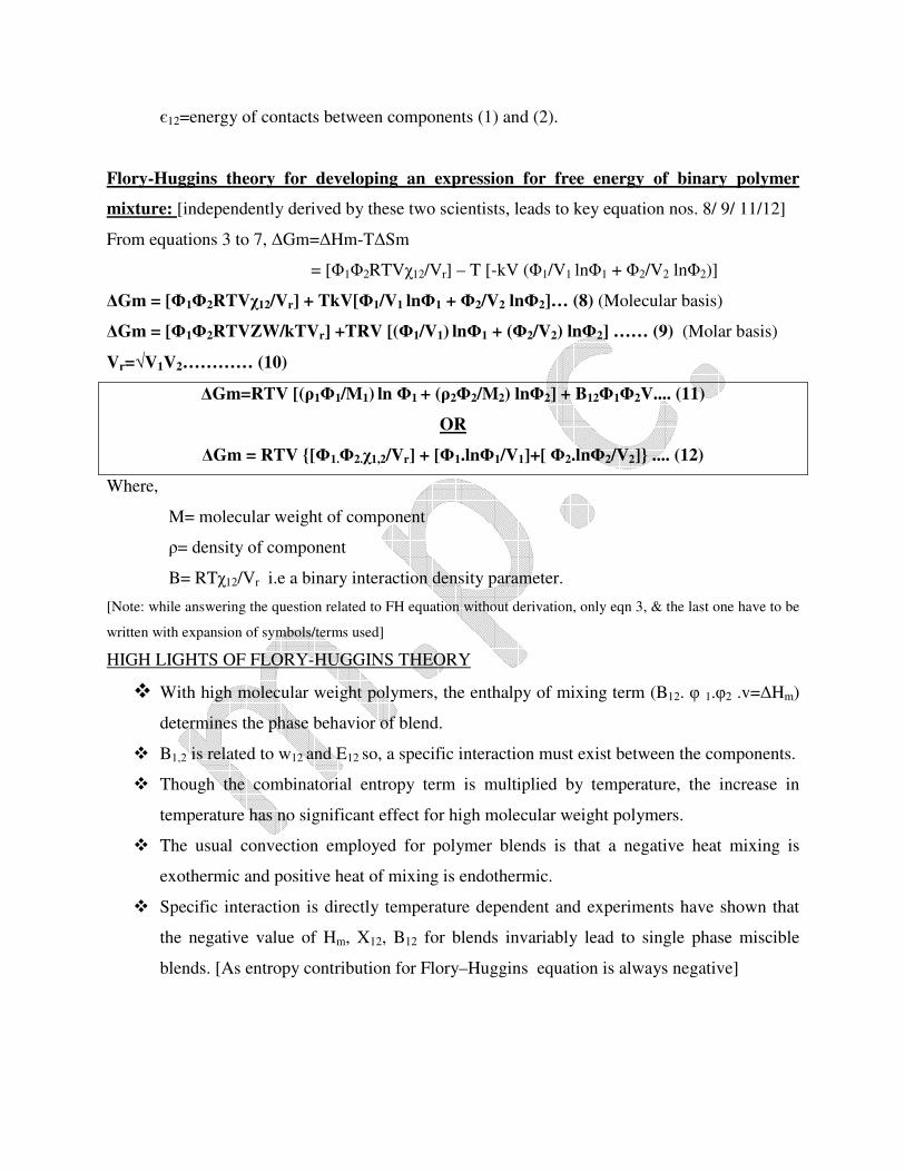
Flory-Huggins theory for developing an expression for free energy of binary polymer

mixture: [independently derived by these two scientists, leads to key equation nos. 8/ 9/ 11/12]

From equations 3 to 7, ∆Gm=∆Hm-T∆Sm

= [Φ1Φ2RTVχ12/Vr] – T [-kV (Φ1/V1 lnΦ1 + Φ2/V2 lnΦ2)]

∆Gm = [Φ1Φ2RTVχ12/Vr] + TkV[Φ1/V1 lnΦ1 + Φ2/V2 lnΦ2]… (8) (Molecular basis)

∆Gm = [Φ1Φ2RTVZW/kTVr] +TRV [(Φ1/V1) lnΦ1 + (Φ2/V2) lnΦ2] …… (9) (Molar basis)

Vr=√V1V2………… (10)

∆Gm=RTV [(ρ1Φ1/M1) ln Φ1 + (ρ2Φ2/M2) lnΦ2] + B12Φ1Φ2V.... (11)

OR

∆Gm = RTV {[Φ1.Φ2.χ1,2/Vr] + [Φ1.lnΦ1/V1]+[ Φ2.lnΦ2/V2]} .... (12)

Where,

M= molecular weight of component

ρ= density of component

B= RTχ12/Vr i.e a binary interaction density parameter.

[Note: while answering the question related to FH equation without derivation, only eqn 3, & the last one have to be

written with expansion of symbols/terms used]

HIGH LIGHTS OF FLORY-HUGGINS THEORY

� With high molecular weight polymers, the enthalpy of mixing term (B12. φ 1.φ2 .v=∆Hm)

determines the phase behavior of blend.

� B1,2 is related to w12 and E12 so, a specific interaction must exist between the components.

� Though the combinatorial entropy term is multiplied by temperature, the increase in

temperature has no significant effect for high molecular weight polymers.

� The usual convection employed for polymer blends is that a negative heat mixing is

exothermic and positive heat of mixing is endothermic.

� Specific interaction is directly temperature dependent and experiments have shown that

the negative value of Hm, X12, B12 for blends invariably lead to single phase miscible

blends. [As entropy contribution for Flory–Huggins equation is always negative]

� Other factor including non-combinatorial entropy of mixing terms is not covered by

Flory-Huggins equation, but plays a significant factor in phase behavior and is explained

in “equation of state theories”.

� Flory-Huggins approach is not directly capable of predicting LCST.

Unit-3

Various parameters that contribute for Miscibility of polymer blends

After the thermodynamic approach of free energy determination for knowing miscibility of

blends, let us see how other parameters contribute for miscibility: (in earlier Units, the list is

mentioned)

Solubility parameter concept for miscibility

For liquids, solubility parameter Sp was defined as square root of cohesive energy density

Sp = (∆Ev/V)(1/2)

Here, Ev = energy of vaporization.

[Sp values ranges from 12(MPa)(1/2) for fluorocarbon gases to 30(MPa)(1/2)for Hg]

While for polymers, many techniques are employed to determine Sp, one example is swelling

parameter i,e. the Sp the solvent at the position which shows highest swelling of lightly x-linked

polymer is considered as Sp of that polymer.

Values of Sp for some polymers:

Polymer Sp

(MPa)(1/2)

PTFE 12.7

BR 16.7

PS 18.7

PVC 20.7

PAN 26.7 to 30.7

� Small (scientist) observed that the Sp of polymers could also be calculated using group

combination approaches as:

Sp = ρ . [∑Fi/M]

as, ρ =M/V it can be written as Sp = ∑Fi/V

Here, F=molar attraction constant

M=Molecular Weight of repeat unit

V=molar volume

� Solubility parameter calculated by such approaches showed that values of PPO and PS are

matching, i.e. 19 (MPa) ^ (½) and says that, with minor contribution of specific interactions

and entropy, this blend is miscible due to matching Sp. If there is difference in Sp then

specific interactions are must for miscibility. The experiments have come up with practical

guide for predicting miscibility based on specific interactions and critical solubility

parameter difference :

∆Sp (MPa)(1/2)

Specific Interactions

If <0.2 Then, dispersive force are sufficient for miscibility

If <1.0 Then, polar forces are required for miscibility

Similarly,

<2.0 weak specific interactions

<4.0 moderate specific interactions

<6.0 strong specific interactions

� Also, the heat of mixing is proposed to be the sum of dispersive and specific interactions

contributions.

∆Hm=Hm(specific) +Hm(dispersive)

� Though the Sp can be used as a guide, it lacks the ability to predict specific interactions.

SPECIFIC INTERACTIONS that play one of the important roles in achieving miscibility:

In order to achieve the ‘negative’ heat of mixing as required by high molecular weight polymers,

specific interactions play a key role. Purely dispersive interactions would not be sufficient, and

hence interactions like hydrogen bonding, acid-base [Laury-Bronsted or Lewis charge transfer],

dipole-dipole, ion-dipole, dipole-induced dipole, ion-induced dipole, π-hydrogen bonding, n-π

complex, π-π complex formation, or etc; are also necessary to achieve miscibility. The relative

strength of these interactions range from 0.4 KJ/mole [London dispersive force/ Wander Waals

force] to 25KJ/mole [hydrogen bonding]. [info: covalent bond’s strength is 100KJ/mole]. The

examples of polymer miscibility attributed to these interactions are as shown below:

Interaction Contributing Groups Examples of polymer pairs

acid-base

Anionic polymer with Cationic polymer

Polyester or carbonyl polymer with Phenoxy

or Polyvinyl phenol

Aliphatic Polyester with PVC

PEO, PVHE with Phenoxy

PEO, PVME with PAA, PMAA

[PVME= POLY VINYL METHYL ETHER]

dipole-dipole

PVF2 with Variuos Poly acrylates, PVAc

ion-dipole

Styrene Sulphuric acid (metal salts) containing

Polymers with PA

π–hydrogen

bonding

PS with PPO

n- π complex

PC with PMMA,

PC with Polyester

π - π complex

PS with TMPC

charge transfer

aromatic nitro polymers with tertiary amine

containing polymers

Characterization of Polymer Blends

[Note: student while answering this unit’s question shall not explain the instrumentation/ procedure/ principle

etc as was learnt in analysis subject previous semester! Only the technique or approach of analyzing blend for

its phase, miscibility, performance, reaction with compatibilizer, and such things shall be highlighted,

preferably with help of sketch, like we did in class. The Idea or basis for using certain techniques for blend

analysis is mentioned below]

• Morphology using microscopy (OM, TEM, SEM, and AFM) various morphologies

saying about blends’ phase behavior has been discussed initially.

• Spectroscopy: UV-Vis, IR and x-rays < idea about change in crystallinity, formation

of new groups, etc can be realized>

• Determination of Tg by DSC or DMA:

• DSC: is another research tool to investigate the polyblends. The most unambigious

criterian of polymer miscibility is single Tg, where temperature is intermediate between

those corresponding to the two component polymer.

Influences of various structural changes are usually associated with changes

with heat adsorption or emission etc and are measured using colorimetry. The sudden change

in the specific heat capacity at Tg is manifested as a step on the temperature v/s differential

temperature curve. The temperature at which this transition occurs is different for different

materials. In physical blend of two polymers, each polymer retains its own transition

temperature and both are observed. On the other hand, the pressure of single Tg for a blend is

indicator of homogeneity on a molecular level and thus mechanical integer. Hence,

measurement of Tg assists determination of compatibility of amorphous or semi crystalline

polymer blends.

NOTE: *The additives also influence Tg

*For highly crystalline polymer this technique is not suitable.

*Relaxation of built-in stress due to mixing/ forming/ cutting/ other process can occur at

Tg and can distort shape of transition; hence preforming or premelting is required.

*For small concentration like less than 10%, the small peak is difficult to resolve and

shift of the major peak is negligible.

*The combination of various techniques is also a necessary for blend analysis.

DMA: Because of excellent resolution of the Tg provided by the DMA through the measurement

of E’, E’’ and tan delta (loss tangent); this analysis technique offers a better means for examining

poly blends. Transitions in semi miscible blends that may be difficult to resolve by DSC are

readily determined by DMA. Generally, for an immiscible blend, the loss modulus (E’’) curve

show the presence of 2damping peaks corresponding to Tg of individual components .

For a highly miscible blend the curve shows only a single peak where as broadening of transition

occurs in case of partially miscible system. [Peak or onset of increase in tan delta; peak or onset

of increase in E’’;]

Spectroscopy helps in study of blends: UV-visible, X-ray and IR:

Electromagnetic (EM) radiation and the interaction with the specific groups of polymer blend as

a function of wavelength (frequency) is an important method to ascertain specific interactions

between interacting species.

The spectroscopic techniques based on molecular vibrations can measure molecular interactions,

such as hydrogen bonds or chemical reactions (with FTIR, Raman, and NMR). However, these

techniques are not very sensitive to the phase separation or dispersion; and are mostly non-

qualitative; therefore, they must be used in conjunction of other techniques.

X-ray photoelectric spectroscopy (XPS): Is commonly employed to determine the surface

composition of polymeric materials, upon X-ray irradiations, the inner-shell electrons can be

emitted & measurement of its kinetic energy can help identify the source material of electron

emission & thus determine the atomic composition of surface.

For e.g. ‘C’ (carbon) of -CH2-; -CF3; -CF2-; -CHF-; etc all show difference in binding energy.

Measurement of diffusion of one polymer into another can be found using thin film. In case of

strong specific interactions, the shift in binding energy can be observed, In case of immiscible

blend, the low surface energy component and can be a check to study miscibility by this

technique.

IR-Spectroscopy: Most important spectroscopic method for determining specific structural

groups in polymeric materials. If the blend has some interactions/reactions; there will be

appearance/disappearance/shift of some peaks in spectrum of blend accordingly.

Transition between vibrational or rotational states of a molecule can be detected by IRS. H-

bonding can be detected by observing the shift in frequency of absorption peak for the H-bonded

unit. Specific group capable of H-bonding includes OH stretching transition around 3600cm^-1;

C=O absorbance around 1730cm^-1; amide group exhibiting N-H & C=O stretching at

3300cm^-1 & 1640cm^-1 respectively. E.g. PC/PBT blend analysis showed ester exchange

reaction.

UV-Visible spectroscopy: In the UV-visible frequency range [180-380-780nm], valance

electrons can be excited & observed. For blends that exhibit electrons transfer complexion

involving electron acceptor & electron donor polymer blends; e.g. Polymer with ester & polymer

with amine group, when blended. These techniques measures optical properties of blends over

the full range.

With the interactions of various polymers, there exists change in energy levels or transition

bands or energy gap etc, that reflects in spectrum. e.g…….π-π* UV band of phenyl groups can

be perturbed by electron donating or withdraw ability of substituent group & data shows changes

in conjugation or conformation of phenyl group. UV-visible spectrum is important for evaluation

of electroluminescent/photo luminescent polymer blend (the one used in LED) to determine

overlap of respective adsorption spectrum & to design material with specific emission as

required for electroluminescent condition.

[Information: though, Tg is the most commonly used property to check miscibility, the Tg is not

a thermodynamic property!]

Unit-4

COMPATIBILIZATION

Compatibilization Methods: Many polymer mixtures are not only immiscible but also

mechanically incompatible. In order to achieve desired property balance, compatibilization is

employed in many commercial polymer blends. Generally, the compatibilization methods

involve an interfacial agent that lowers the interfacial tension between the components leading to

a more uniform blend with smaller particle dimension, as shown below:

The interfacial agent allows for improved mechanical compatibility by achieving improved

interfacial adhesion between phases. The agent can be considered as "polymeric surfactants" that

concentrates at the interface & stabilizes the morphology, by preventing the coalescence which is

one of the major problems in achieving small particle size dispersions got by shearing the

incompatible blends.

Compatibilization Approaches include:

1. Introduction of specific interacting groups.

2. Insitu polymersiation grafting.

3. Addition of non-reactive ternary homo-polymer that adheres to both phases and

concentrates at interface.

4. Adding non-reactive ternary block co-polymer comprised of units as that blend polymers

or blocks that adhere to both phase.

5. IPNS of X-linked systems.

6. Reactive compatibilization (effective, widely used both for commercial and research

purposes).

Some Specific examples-

1. Introduction of specific interaction groups: Rather than increasing the micibility to

greater extent, this technique improves dispersion and mechanical properties. Example to

this approach could be to attach small amount of proton acceptor to one component and a

proton donor to another component of the blend. Examples-

a) Less than 0.5 wt% of acidic or basic monomers grafted to PE/PP to yield improved

mechanical compatibility.

b) PS-co-4-Vinyl benzoic acid and poly butyl methacrylate-co-4-vinyl pyridine.

c) PVOH/PE is immiscible, by introducing vinyl amine and acrylic acid respectively,

properties were improved with transparency.

d) Sulphonation of PEEK yielded miscibility with PA6 due to H-Bonding.

e) PS with para substituted hexa fluoro iso propanol (expanded PS), its miscibility

range include series of polymers: Poly Acrylates , PMA , PEO, PC, PVAc, PVMK,

etc

[Note: the required property improvement, Tg values, FTIR peak shift, etc were evidence for

compatibilization]

2. Addition of non-reactive ternary homo polymer: The poly hydroxy ether of BPA

(phenoxy or PHE) has been noted in various studies which have provided improved

interfacial adhesion between immiscible or marginally compatible blends. E.g.-

a) The above polymer with PSF/ABS improved dispersion, increased impact strength and

uniformity of injection molded surface.

b) and with PBT/PC showed 2 Tg but improved transparency

c) PCL with SAN/PC

d) PC with PPO/PBT

e) Chlorinated PE with PVC/LLDPE

f) CPE with SAN/EPDM

3. Addition of non-reactive ternary co-polymer: Non-reactive ternary systems include

random, graft or block copolymers offering miscibility or good interfacial adhesion in blends.

a) Poly (styrene- hydrogenated diene - styrene) block copolymer with PS/Polyolefin blends.

[Not only block but also sometimes random copolymer addition to binary blends

involving copolymer with structural units equal to or similar to the blend components, or

with specific interactive groups capable of non-reactive interaction with one or both of

the blend components comprise another ternary polymer addition approach.]

b) EPR with HDPE/PP gave synergistic impact strength.

c) Graft copolymer addition with the graft copolymer comprised of a main chain of one

component and the graft of other component of blend provided an effective ternary

addition method. NR grafted with Styrene compatibilised the NR/PS blend showing

decreased domain size and increased melt viscosity.

d) EVA grafted MMA with PVC/EVA

e) Block copolymer will concentrate at the interface and allow for improved adhesion

between phases as shown below:

Figure: Concept of compatibilisation using AB or ABA block copolymer

SEBS (styrene ethylene butylene styrene) block copolymer with the atactic

polybutylene/PE blend (i.e. at.PB/PE) or with at. PB/PP blend shows great increase in

mechanical properties like impact strength and elongation at break. (SEBS with syn.

PS/HDPE blend showed no improvement because crystallization of syn. PS at interface

segregates SEBS out of blend domain.) SBS, SIS, SBR (random) were all good

compatibilizers with PP/PS but properties vary with each type.

1. In-situ Polymerization: involves covalent bonding between the constituents resulting in

graft or block copolymerization allowing for interfacial stabilization. Impact PS is a specific

commercial example where this concept has been very important

a) Polymerization of styrene in presence of butadiene rubber allows for graft

copolymerization formation along with rubber x-linking. The resultant phase separated

rubber particles yield toughening of the brittle PS matrix.

b) Emulsion particle of BR are used in emulsion polymerization of SAN copolymerization

to get ABS.

A compatibilisation technique specifically suitable for emulsion polymerization involves the

in-situ polymerization of polymer in the presence of previously polymerized polymer. As

applied to the emulsion polymerization, this is typically referred to as core-shell

polymerization. The procedure involves the initial polymerization of seed particles; the

addition of other monomers can result two distinct results:

i. One result involves swelling of monomer in the particles followed by phase

separation once a critical molecular weight is achieved due to immiscibility of

polymers.

ii. The other result would involve the formation of 2nd polymer as a shell around the

seed core particles.

The 2nd process would be expected if the initial polymerization occurs in the aqueous phase,

followed by adsorption on the core particle surface once the oligomeric molecular weight

reaches limiting water phase solubility or limiting water phase water phase stability values. In

practice, both process can occur and often do so simultaneously, yielding a resultant morphology

ranging from true core shell to particles with both phases equally distributed in a inter-

penetrating morphology. If x-linking is provided for both polymers, then this procedure would be

a sub set of IPNs. Variations in morphology are illustrated below:

Fig. core shell polymerization morphologies

Variation is due to change in- component type, composition ratio, core particle size,

particle surface polarity, mode of monomer addition, staged ratio, saturation of polymer formed,

chemistry of polymerization and cross linking of both polymers, inter facial energy, etc;

5. Reactive compatibilization: This approach is used in case of highly immiscible blends

to get a good mechanical compatibility. It involves introduction of a reactive site onto a

polymer chain identical or similar to one blend component capable of reacting with the

other polymeric component. The resultant graft co-polymer will as usual concentrate at the

interface and reduce to interfacial tension, yielding improved dispersion, domain size

reduction and improved mechanical properties over the binary blend. A variation of this

method can involve addition of polymer miscible with first component capable of reacting

with the other component to form a graft co-polymer.

a) PS-co-(minor amount of) MA blended with PPO/PA6 and resultant PS-g-PA6 copolymer

will be at interface as PS prefers PPO.

b) PA6/VLDPE-g-MA showed elongation at break more than 120% of the previous binary

blend.

Following table gives examples of groups used and reactive sites for achieving reactive

compatibilization of blends- (remarks: all of the below systems form graft copolymers)

Group Method of usage Sites and

Polymer e.g.

MA Grafted onto poly olefins or monomer with

styrene copolymer or ter polymer.

* amine of PA

*hydroxyl of polyester

Acrylic acid Graft or copolymer *amine of PA


Oxazoline Functionalization with polymer *amine of PA

*acids of polyester

NCO Graft or copolymer *amine of PA


*acid of polyester

Epoxy Incorporation via glycidyl methacrylate

containing copolymer or as grafted side

group.

*amine of PA


*acid of polyester

Note: each of these systems can be grafted to poly olefins or unsaturated polymer by free-radical

grafting techniques employing a peroxides.

Descriptions of chemical reactions are as follows:

A specific subset of this method involves reactive extrusion (discussed under blending

equipments)

6. Inter-Penetrating Polymeric Networks (IPN): this method involves compatibilizing the

diverse polymers by sequential or simultaneous polymerization of polymer networks. The

interlocking rings of polymers, which are referred to as catenane structure, would make the two

polymers stay together (i.e. compatible). The system consist single phase behavior of monomer–

monomer or monomer–polymer mixtures with appropriate x-linking additives being used. Upon

polymerization of monomer/s, the incompatibility leads to phase separation but the network

prevents complete localization. It’s not essential that the two polymers should have covalent

bond between each other but essentially the chain should get interlocked leading to mechanical

adhesion as shown below:

Fig. interpenetrating network of flexible and rigid polymers

Fig. Catenane structure: interlocking polymeric rings

Methods of producing such IPNs include:

I. Sequential IPN- e.g. PDMS/PMAA

II. Simultaneous IPN- e.g. PU/PMMA

III. Semi IPN- e.g. PU/PDMS

Note: the TP IPNs comprised of interpenetrating phases such as- block copolymers, ionomers,

crystalline polymers etc. are formed by physical x-linking (specific interactions) and not by

covalent bonding or chemical x-linking and hence sometimes may not be discussed here instead

under other types or under specific interactions or under cross-linking phases.

7. Other types:

I. X-linking between phases: It is used mostly with phase separated elastomeric systems

(for tyre related applications) using sulphur or peroxide X-linking which leads to covalent

bridging between two phases and thus assuring proper translation of stresses from one

component to other. E.g. Co-X-linked compatabilized elastomeric blends i.e, co-

vulcanized blends of EPDM/NR.

II. Polymer-Polymer reaction: the interchange reactions between different polymer can lead

to compatibilization with or without catalyst and often to miscibility between polymers

that are typically phase separated. E.g.-

a) Ester interchange between polyester like PC/PET, PET/PBT, polyarylate/PC, PC/PTT

etc.

b) Trans esterification between PHE/PBT, EVOH/PLA.

c) Trans amidation between polyamide like PA4,6 / PA.

d) Ester-amide interchange reaction between polyester and polyamide like PET/PA66.

e) Acid-amide interchange reaction between SAA/PA6 (SAA=styrene acrylic acid).

III. Additional method of compatilization:

a. Solid state shear pulverization– involves application of high shear or extrusion

below the Tm or Tg to yield a fine powder. Chain scission resulting in free

radicals at the chain ends allows for potential of block co-polymer formation at

the inter-phase when a polymer blend is employed. E.g. PP/PS; PS/PMMA.

b. Use of coupling agents– zirconate and titanates with PC/PET and recycled

polyolefins/LCP. Silane coupling agent with PP/PET.

c. Inorganic fibres and fillers: nano fillers, functionalized clay particles, etc have

compatibilized many blends. E.g. PC/PMMA, PA6/ABS, PMMA/PVAc, etc.

Toughened Polymers (via blending)

Toughened thermoset:

Background: Most of the thermosetting resins develope dover the last decade are largely used as

matrices in fiber-reinforced composite for aerospace industries. As aircrafts are pushing towards

greater speed, composites with high strength to weight ratio would be preferred. Also these

resins are capable of withstanding elevated temperature applications via increased rigidity &

increased x-linking to form networks. However, in almost every case the same network which

provides the high temperature property & strength would also inhibit molecular flow. Thus,

making the material possess low toughness.

Following fig. shows example of some TS resins relating their Tg with toughness.

Despite their brittleness, TS resins are important for use in fiber composites because with the

current system of its manufacturing, the equipments suit TS resins for processing and fabrication

which does not suit TP; and also toughening the existing thermosets would be more attractive

and economical than developing a new system.

The fracture toughness of TS resins of 50 to 300 J/m² is marginally higher than inorganic glass.

However, by incorporating toughener into resins such as epoxy the toughness level can be

brought into the line with some TPs.

Though, most of the work w.r.t. toughening a TS resins involve incorporation of soft elastomeric

substances into resin matrix; but as the high temperature requirement becomes more critical,

incorporation engg. TPs as toughening agents has become more popular.

CE and BMI resins have similar processing characteristics like epoxy but posses better

mechanical properties with max. service temperature between 150˚-250˚C (i,e between the

epoxy and poly imide respectively).

The compatibility requirement of blending the elastomer with TS resins is different from TP

blending. The elastomers are usually low mol.wt. liquids and are capable enough to dissole &

disperse in the resin monomer or lacquer on storage, but phase separate out during curing of the

resins. Whereas, in blend of TP with TS, the significance of entropy factor is greatly diminished;

consequently the miscibility influenced by the difference in value of solubility parameter.

Most of the TPs used are usually high temperature enng. TPs like PES, PI , PAS; which are

either incorporated by hot melt blending or by solution blending. A small degree of chemical

reaction between the TS resin and modifier (I,e with end group of engg. TP) is often desirable for

effective toughening, sustaining the side effect of solvent on overall properties.

[Note: For fiber composite applications, the particle size of finely dispersed modifier must be

below 8micron, which is equivalent to average fiber spacing.]

Toughening of TS resins with soft inclusions:

It is mainly for low temperature applications that elastomeric particles are used for toughening

TS. One of the majorly used toughener is CTBN rubber <Carboxy terminated butadiene

acrylonitrile >.

Ex 2: usage of phase separated acrylic elastomers suspended in uncured epoxy via mechanism of

stearic stabilisation showed a much higher toughness (peel strength).

Ex 3: PMMA-g-NR copolymer usage showed increase in fracture toughness of both low and

high cross-linked density epoxies.

Ex 4: Copolymerisation & chain extension reaction also gave tougher networks < in most cases

reduction in Tg was observed >.

Ex 5: Developing SIPNs (i.e. Semi IPNs) using TPs resulted in phase separation yielding good

toughness & processability along with other physico mechanical properties.

Toughened TP’s: Commodity plastics such as PE, PP, PS, PVC, etc. Make up a large portion of

total tonnage plastics being used mainly for non load bearing applications i.e., many of consumer

products. However efforts are made to improve their toughness, wide range of temperature

applications, stiffness with retaining its lightness via blending instead of developing new

polymers or using various ingredients in compounding.

The efforts are in developing heterogeneous polymer i.e., 2 phase systems which are

referred as toughened TPs. Literature reveals usage of engineering plastics like PPE, PPS, PC,

PEK, PEEK, LCP & their copolymers; & rubbers like EPDM, BR, NR, & their copolymers in

majority, for increasing the toughness of commodity plastics.

Majority of such toughened TPs forms immiscible blends with increase in impact

properties but there exist a need of compatibility at interface via copolymer technique or reactive

melt processing- REX & RIM.

1. MMA-g-rubber with PMMA, PS, HIPS, ABS, etc.

2. EPDM with PP/HDPE

3. PS-Co-MA with PA6/SAN

4. PC/PS, PEEK/PS, PC/PMMA, etc

5. PP/NR with slight cross linking.

Note: Usage of thermotropic LCP’s with many engineering plastics not only enhanced

toughness but also ease of processing & also stiffness in flexible polymers because of their

unique melt viscosity of blends that lubricates polymer melt and lowers viscosity of blends.

Ex: LCP/PC, LCP/PA6

Mechanism of toughening:

Most of TS’s & few of TP’s fail in brittle manner under tensile loading but some

polymers will exhibit ductile behaviour under compression (even some of the highly cross linked

epoxy system). The inherent ductility of a polymer matrix depends on its ability to undergo

plastic deformation during stress (of course influenced by test conditions & geometry).

Incorporation of toughness can increase the fracture resistance of base polymers by:

I. Enabling plastic deformation to occur in the matrix.

II. Increasing the plastic deformation which is occurring in the matrix.

III. Undergoing fracture themselves.

Depending on nature of base polymer & toughening polymer.

Toughening mechanism in TP’s:

It is well established that rubber particles with low modulus act as stress

concentrators in both TP & TS resins enhancing shear yielding and/or crazing, depending on the

matrix nature.

Shear yielding in a polymer matrix involves macroscopic drawing of material

without change in volume at 45◦ to tensile axis. Depending on polymer, the yielding may be

localized into shear bands or diffused throughout the stress region. It is initiated by a region of

high stress concentration due to flaws or polymeric inclusions such as rubber particles.

Crazing, on the other hand, is a more localized form of yielding and occurs in planes

normal to tensile stress. These are wide at crack tip that are interconnected by highly drawn

fibrils which also form the craze walls and contain approximately 50% of voids photo 200Ao.

TEM micrograph showing crazes of tensile fractured specimen.

Nucleation happens at interface of high stress concentration caused by in-homogenity such as

flaws and polymer inclusions. Theory of multiple crazing in rubber toughened TP systems:

Crazes are initiated @ points of maximum principle strain which are usually near the equator of

the rubber particles and then propagates outwards along the plane of maximum principle strain.

It is terminated when stress concentration falls below the critical level for propagation, or when a

large particle/ other obstacles is encountered. Thus the rubber particles are able to control craze

growth by initiating and terminating crazes a shown in the figure.

Later it was proposed (by Bucknall and Smith) that shear yielding and massive crazing are the 2

energy absorbing mechanism in rubber modified plastics. According to that, areas of stress

concentration produced by the rubber particles are initiation sites for shear band formation as

well as for crazes and that shear yielding is not simply an additional deformation mechanism, but

an integral part of the toughening mechanism. Since the molecular orientation of shear band is

normal to craze growth. Therefore as the number of shear bands increases, the length of newly

formed crazes will be low and consequently a large number of short crazes are generated.

Note: The process of "voiding" as one of the toughening mechanism has been reported as

successful approach from many researchers for different materials.

Toughing Mechanisms in TS Resins:

Due to range of x-link density and matrix ductility (with different TSs) there is no one

generalized mechanism that can be used to describe toughening of TSs and hence it is a

combination of number process as mentioned below:

1. Tearing and ductile drawing of dispersed phase- a crack in rubber toughened epoxy

propagates through the brittle epoxy matrix and leaves the particles bridging the crack.

This deformation is also applicable to TP toughened TS in which particles are well

bonded to the matrices.

2. Crack tip blunting of resin matrices- the hydrostatic tension generated in well bond

rubber particles due to curing & cooling, along with load on specimen, develops tri-axial

stress @ crack tip leading to cavitations in particles or @ particle matrix interface. This

increases the stress concentration of particles and also allows shear band to grow

promoting yielding as a consequence of it. The whole process creates plastic yield zone

containing distorted and voided particles that produce a crack tip blunting effect releasing

the stress @tip and delaying crack propagation which eventually end up in voided plane.

3. Crack pinning mechanism of impenetrable and semi penetrable particles- usually in the

filled systems.

[Note: particle size and processing also influence toughness]

Unit-5

Interpenetrating Polymeric Networks (IPNs)

These are unique type of polymer blends, usually synthesized by swelling a cross-linked polymer

with a second monomer together with cross-linking and activating agents and polymerizing the

monomer in-situ. The term was so adopted because both networks were being interpenetrating

and continuous throughout the entire macroscopic sample (analog to worms eating out

independent tunnels in an apple). Even though in some cases the two components are

incompatible, they remain intimately held, and shows phase domain sizes in the order of

hundreds of angstrom.

If one polymer is elastomeric and other plastic, at temperature under consideration, then

the combination tends to behave either as reinforced rubber or as impact resistant plastic.

Types include:

a. Sequential IPN.

b. Simultaneous IPN (SINs).

c. Semi IPN

d. (TP) Elastomeric networks (IENs).

e. Latex IPN.

f. AB cross-linked copolymer.

Brief description of all 6 types:

a. Sequential IPNs involve synthesis of a polymer network followed by addition of

monomer+ X-linker which dissolves and swells the 1st polymer network. Then the 2nd

monomer polymerizes and phase separates but the chains get interlocked due to X-

linking.

b. In SINs, both the networks are formed simultaneously, like- addition polymerization of

one component along with condensation polymerization of other component i.e. it needs

independent, non- interfering polymerization reactions that can be run at same time under

same overall conditions. It involves monomers or reactive systems.

c. Semi IPNs involves one X-linked polymer and another non X-linked polymer. Two

variations of this class involve;

� Addition of monomer/s to X-linked network followed by polymerization.

� Addition of monomer/s and X-linking moieties to a non X-linked polymer.

d. IENs are prepared by mixing and coagulating two different kinds of polymeric emulsions

followed by single X-linking reactions (using single X-linking agent) resulting in 3D

mosaic structure.

e. Latex IPN is prepared through emulsion polymerization by taking a cross-linker and

activator and polymerizing monomer on the original particles.

f. AB cross-linked copolymer: In this special kind of graft copolymer, both ends of

polymer-2 are grafted to different polymer-1 molecules, causing one cross-linked grafted

network to arise.

Detailed discussion of the 6 types mentioned above consists- synthesis, morphology, properties

& behavior:

Sequential IPNs: The synthesis of IPN requires a cross-linked polymer-1 which may be rubber

or plastic. This network-1 may be synthesized and cross-linked at same time by using chemicals

like- ethyl acrylate (EA) and tetra ethylene glycol di-methacrylate (TEGDM), using UV-photo

polymerization and benzoin activator. (When plastic is used, the term inverse IPNs is employed

is some cases because initially rubbers were used.)

Alternatively, the linear polymer may be prepared first and cross-linked by subsequent reaction

like subjecting BR films containing di-cumyl peroxide to heat and pressure.

The second network was synthesized in all cases by swelling in a controlled amount of

monomer, allowing ample time for diffusion so that swelling was uniform, followed by photo-

polymerization or thermally initiating peroxide species. Example: styrene +0.5%TEGDM

+0.3%benzoin swelled into PEA to equivalent weight resulting in 50/50 PEA/ PS (being opaque,

white and leathery).

Although both networks may be visualized as continuous, their milky appearance hints at a more

complex morphology. In-order to characterize the morphology, the elastomeric portion of the

IPNs was stained selectively using osmium tetroxide. IPNs exhibit a characteristic cellular

structure, where the first component makes up the cell wall and the second forms cell content.

E.g. cis-PB/PS and PEAB/PS. Though the cellular structure have already been observed with

graft polymerization, here in IPNs the cellular structure pervades entire macroscopic sample

rather than just discrete regions.

Since the chains are cross-linked to each other, the opportunity exists to form a continuous

network throughout the cell walls, which connects the cell contents. The props structure of the

fine dispersed phase within the cell wall is as shown schematically below:

Fine structure within domains for an IPN

The solid black circles represent cross-links. Distance between phase domains is less than half

the chain contour length between cross-links in the network, thus permitting phase separation to

occur; at the same time some network segments provide the requisite inter connection between

phase domains.

Simple homo polymers and random co-polymers exhibit single sharp glass transitions, but

polymer blends and in particular IPNs show two such transitions for each phase. The intensity is

related to composition and phase continuity, while shifts and broadening of transition indicate

extent of molecular mixing [in contrast, EM (electron microscopy) shows phase size and shape

in major, and gives only slight indication of extent of true molecular mixing].

Dynamic mechanical spectroscopy (DMS) techniques yields loss modulus compared to static

mechanical tests which just gives storage modulus. DMS and EM techniques provide

complementary info on two phase materials: the former is a sensitive indicator of the extent of

molecular mixing, while the latter shows the size and shapes of phase domain.

The ultimate utility of any material lies in its performance. The reinforcement obtained by IPNs

exhibit its good ultimate mechanical behavior. Example: The ultimate elongation and stress at

break in case of random (cis-trans mixture) PBD homo-polymer is increased by three to five

times with addition of PS network.

IEN: It is a special term used to designate the formation of IPN from 2 distinguishable lattices

subsequently mixed, coagulated and X- linked. Except for X-linking reactions, the IENs are

topologically very similar to the mixed lattices.

Lattices of urethane-urea (U) and poly-acrylate (A) over the composition range 10/90 to 90/10 by

weight were initially studied extensively. The lattices of the A component were X-linked

together by reacting with double bonds using Sulfur; The U polymer being self cross-linking

with temperature because of free hydroxy groups; the IEN case was achieved.

As polymers were synthesized separately, the inter-molecular grafting may be entirely absent in

many cases, and as a result of X-linking reactions, each phase consist of only a single molecule

of infinite molecular weight.

Morphological studies says that only very limited true molecular interpenetration takes place

with IENs and that too limited to the phase boundaries; Therefore the main interpretation is of

the phases rather than the molecules and shows 2 transitions when characterized.

Semi IPN: Materials having one linear and one X-linked polymer. Specifically it is a graft co

polymer in which one of the polymers is X-linked and other essentially is linear. The 2 semi

IPNs being inverse of each other may be distinguished as:

a) A semi IPN of first kind, with polymer-1 in network form and polymer-2 linear.

b) A semi IPN of second kind, with polymer-1linear and polymer-2 X-linked.

The mechanical property of first kind is better than second kind. Further, increasing the X-link

density of polymer-1 produces finer phase domains. It is also possible to obtain domains that are

too small to impart maximum toughness.

If both the phases are X-linked, then there will be 2 Continuous phases with better properties

than the 2 types discussed before.

AB X-linked co-polymer: Also called as joined IPN, got by grafting different polymer-1 at the

ends of polymer-2 leading to one X-linked grafted network. Thus ideally, one molecule is

generated for AB X-linked copolymer compared to the 2 molecules that are ideally generated for

the IPNs and IENs. Note that polymer-1 is grafted primarily to polymer-2 and it is not

cross-linked to itself.

e.g.1: Castable polyester resin synthesized by polymerizing styrene monomer in an

unsaturated polyester solution are AB crosslinked copolymer characterized by short chains

of length upto 10mers between grafts. E.g.2: Epoxy resin cured by reaction with a

polyamide.

A new technique for making AB cross linked copolymer involves crosslinking of suitable

polymer-1 with chains vinyl polymer-2 by reaction of halogen containing groups in

polymer-1 with an organo metallic derivative (e.g. MO(CO)6) in the presence of monomer-

2. The reaction scheme is as shown below:

The crosslinked networks so produced shows 2 Tg when analyzed by dilatometric

technique indicating phase separation.

SINs: the art of simultaneously synthesizing 2 polymers has already received attention

and also shows excellent mechanical properties. A simple example includes an epoxy

resin (step growth mechanism) with an ethyl acrylate formulation (free radical chain

addition). When a tertiary amine was used to cure the epoxy, minimal interference

occurred between the 2 reactions.

If the above reaction was photo chemically initiated and the condensation reaction was

thermally controlled , the 2 reaction rates could be adjusted at will over a wide range.

Starting with a mixture of the 2 monomers, application of both heat and light resulted in

both networks forming together.

The SINs reacted together, had a controlled degree of phase separation as indicated

by intermediate turbidity levels and were apparently superior in tensile strength to

those reacted sequentially (i.e. 2050 lb/inch2 v/s 940 lb/in2 ).

Latex IPNs: Both the networks formed will be on each particle of emulsion system forming

an array of micro IPNs. Due to the thermosetting nature of sequential (bulk) IPNs, they have

one important drawback i.e, lack of processibility. Whereas, IPNs prepared by means of

emulsion polymerization techniques may offer considerable processing advantages

because the thermosetting characteristics are limited to individual microscopic particles

{therefore I/M, film formation by casting/ painting, etc could be used}.

Only few latex IPNs have been developed successfully. Latex IPNs of methacrylics &

acrylics display high values of tanδ over a broad temperature range.

Latex IPNs include many variables like: overall composition, x-link density,

order/preparation, size of final latex particle, etc. Latex semi IPNs of both kinds have been

developed & investigated. Recall the core-shell morphology discussed before.

Blends case studies:

1. PPO/HIPS:

Blend system of Poly (2, 6-Dimethyl-1, 4-Phenelyne oxide) and High Impact Polystyrene.

The engineering Plastic PPO’s properties was extended along with cost reduction & ease of

processing by using the commodity PS, however it lacked toughness in some cases. Hence, the

HIPS was opted to offer excellent toughness. Blend system is compatible across the entire range

of compositions and temperatures; characterized by single Tg. The combination maintained high

tensile modulus and good impact resistance over a wide temperature range. It has good electrical

properties but not flame retardant (can be improved by compounding). Typical compositions of

PPO/HIPS blends are 40-85% w/w for achieving a complex balance of properties. Commercial

applications that were widely seen are heat resistant electrical connectors, exterior automobile

parts, etc. The best method for productions of PPO/HIPS parts was either by vacuum

thermoforming or injection moulding.

[Rubber types used in one of the component HIPS include high cis and low cis

polybutadiene, EPDM rubber and SBS block copolymers. Optimum impact properties occurred

at with an average rubber particle size of approximate 2µm or less. A Core-shell morphology and

the addition of very small rubber particles (0.3µm) improve the properties.]

Usually melt blended, as developed by GE! Even till the present day, these blends are prepared

continuously using twin screw extruders. The flow chart shown in figure below signifies the

preparation of PPO/HIPS/MBS blend system for improved mechanical properties [the use of

ternary component, i.e. MBS enhances properties].

The twin screw extruders used had respective zone temperatures from 1-3 as, 265oC,

270oC, 280oC and 275oC at the die. The injection moulding machine used the following

temperature profile: 110oC at the hopper, 255oC at all zones of the barrel and 90oC at the mould.

Some commercial grades:

Noryl Gen. grade GE Plastics

Luranyl IM grade BASF

Applications:

Computer housings, TV components, Keyboard frames, Electrical component frames and

chassis, Headlight housing, Pump housings and impellers, Valves and pipes.

2. PC/ABS:

Blend of Bisphenol-A Polycarbonate & Acrylonitrile-Butadiene-Styrene terpolymer. PC is

characterized for its high modulus, high toughness, high impact strength and difficult

processability, due to its high melt viscosity. (ABS) is a rubber toughened thermoplastic,

characterized by its notch insensitivity and low cost. On the other hand, the limitations of ABS

are: poor flame and chemical resistance, and low thermal stability. So, in order to compensate the

limitations of each polymer i.e. PC and ABS and according to the need of properties, PC/ABS

blends are made.

The production of the PC/ABS blends started on 1977. The addition of ABS to PC minimizes its

drawbacks without affecting its superior mechanical properties, and also generates other useful

characteristics, such as glossiness and low temperature toughness.

Both polymers are dried in vacuum for 24 h before processing. Dry PC/ABS mixtures with 10-

90/90-10 weight compositions are prepared in a two roller mixer & pelletized. 80:20 is

commercially available. PC and ABS are not completely miscible; many researchers use a

variety of compatibilizers to improve the compatibility. Ordinarily, three types are considered to

reduce the interfacial tension between PC and ABS resin, including block or graft copolymers,

nonreactive polymers containing polar groups and reactive functional polymers. Many

researchers have used: SBS, ABS-g-MA, methyl methacrylate-butadiene-styrene (MBS) and

styrene-maleic anhydride (SMA.

Properties

• ABS gives the material excellent processing properties and PC gives it good mechanical

properties, such as good ductility and high maximum use temperature.

• Both components of blend are amorphous.

• As with most amorphous polymers, the chemical resistance is not so good.

• Easily injection moldable, but also processable using extrusion, blow molding and

thermoforming.

• PC/ABS blend offers good flow and excellent impact. Low temperature ductility.

Applications

• Automotive application: Instrument panels, grills, interior and exterior trim.

• Telecommunication: mobile phones.

• Medical: housing for (electronic) medical equipment.

• Electrical: Housing for electronic devices, electricity meter housing, switches, plugs and

sockets. housings for microwave ovens and components for washing machines and dryer.

• Office equipment: housings for computers, monitors, copiers and printers.

• Middle console, lower instrument panel, pillars, knee bolster, overhead console, blow

molded seatbacks in automotive applications.

• TV frames, laptop monitor enclosures, potable hand held devices, LCD panels, keypads,

adapters and chargers, mobile phone bodies in electronics application.

polymer blends and alloys course outcomes · polymer blend (or binary system). • binary=2,...

Documents